Physics Informed Structural Load Aware Work Path Planning for a Tilt-Rotator Excavator Using Multibody Dynamics and Dueling Deep Q-Learning: A Numerical Case Study

Abstract

A tilt-rotator increases the reachable workspace of a hydraulic excavator, but its configuration also changes structural load paths. This study developed a structural-load-aware work-path planner for a 14-ton excavator using nominal analytical soil loads and an experimentally correlated multibody dynamics model. A full-factorial combination of five tilt angles, five rotation angles, and nine excavation positions yielded 225 candidate motions. The 147 retained motions had predicted peak stresses of 98.5–149.0 MPa. These stresses informed action features and reward penalties in an action-conditioned dueling deep Q-network. Excavated cells became non-traversable holes; the planner incorporated in-place turning and conditional posture-repeat constraints. In the 9 × 9 obstacle environment, the stress-informed agent’s selected route required 44 actions and 452 s of simulated time, compared with 47 actions and 458 s for its stress-uninformed counterpart; cumulative peak-stress indices were 3158.0 and 3361.8 MPa, respectively. In the 5 × 5 environment, its route required one additional action and had a 4.2% higher index. A 21 × 28 site-derived numerical environment was completed in 453 actions, including 280 excavations. The method supports comparative structural-load assessment for construction-machinery safety and future integration with machine-stability criteria. These single-seed comparisons neither establish statistical superiority nor validate machine stability.

1. Introduction

Hydraulic excavators perform material removal through strongly coupled machine motions and soil-tool interactions. Automation research has consequently addressed bucket-trajectory generation, digging control, earthwork scheduling, and coverage planning using simulation, optimization, and reinforcement learning (RL). A systematic review of RL in construction engineering nevertheless identified generalizability, method selection, and validation as continuing challenges [1]. These issues become more pronounced when an attachment introduces additional degrees of freedom and when task-level efficiency is not the only engineering objective.

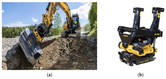
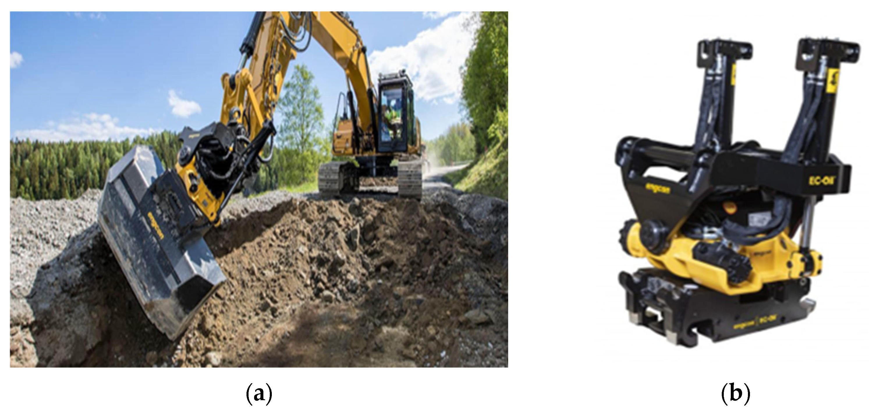
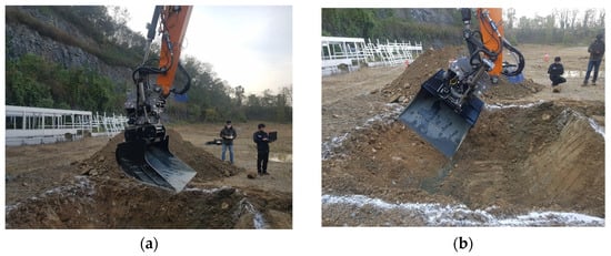
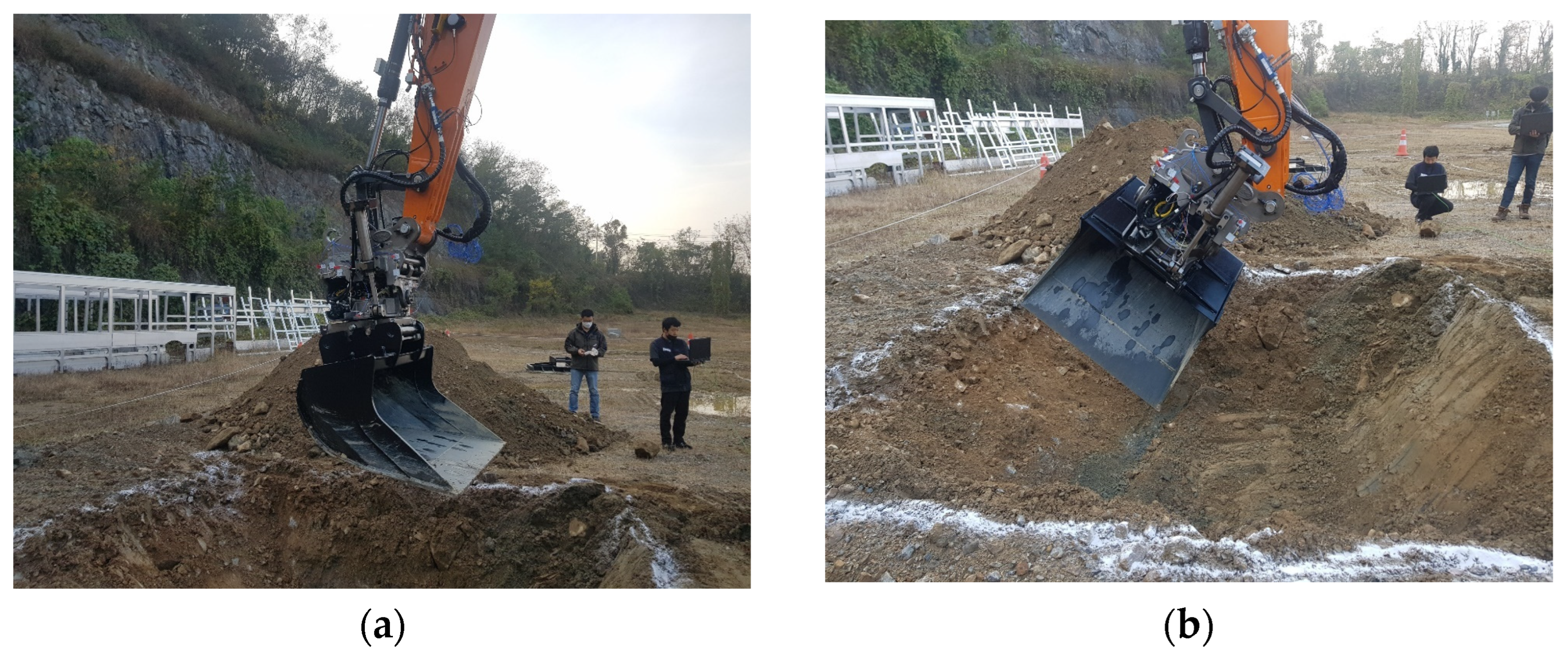
A tilt-rotator adds independent tilting and continuous rotation between the excavator arm and bucket (Figure 1). These motions reduce the need to reposition the carrier and enable oblique or lateral excavation. The same kinematic flexibility, however, expands the set of admissible attachment configurations. Because tilt, rotation, and excavation direction modify the load-transfer path through the attachment, two motions that remove the same soil cell can produce different dynamic stresses [2]. A work-path planner that observes only distance, time, or completion can therefore select a kinematically feasible but structurally unfavorable motion. Construction-machinery safety and stability assessment therefore requires consideration of configuration-dependent loading alongside machine-level stability. The present study addresses the structural-load component of this assessment.

Figure 1. Hydraulic excavator and tilt-rotator used as the mechanical basis of the study: (a) excavation with a tilt-rotator and (b) tilt-rotator attachment.

Existing work has demonstrated complementary approaches to autonomous excavation. Huh et al. used expert data and terrain point clouds for learned bucket-trajectory generation [3]. Physics-informed trajectory planning has incorporated system dynamics and mechanical constraints [4], and physics-guided deep reinforcement learning has incorporated machine-specific stability information into tunnel-boring-machine operation [5]. Autonomous excavation planners have combined global pose selection, local excavation decisions, and digging trajectories [6]. Soil-adaptive RL has addressed uncertain interaction properties at the control level [7], and multibody-system simulation has been coupled with RL for automated excavator operation [8]. At the planning level, RL has been used for dynamic cut-and-fill allocation [9], coherent excavation sequences [10], realistic three-dimensional operational simulation [11], and earthwork planning with heterogeneous construction equipment [12]. Complete-coverage algorithms have also accounted for excavator geometry and turning constraints [13], whereas whole-body planning has coordinated the coupled motions of articulated excavators in complex terrain [14]. RL-based energy management has further demonstrated policy optimization for hybrid construction machinery [15]. These studies primarily optimize feasibility, coverage, cycle time, energy, or motion quality. Configuration-dependent dynamic structural response has rarely been exposed directly to a work-path policy.

Our earlier study established the mechanical foundation for such integration [16]. A multibody dynamics (MBD) model of a tilt-rotator excavator was correlated against vibration measurements, with an average dominant-frequency error of approximately 4.3%. That study also demonstrated the feasibility of supplying dynamic-stress information to an RL planner. That study, however, used a simplified excavation load, a smaller tilt-rotation domain, and a basic 5 × 5 environment. The present article cites that work explicitly and does not claim the original vibration test, model correlation, or initial feasibility demonstration as new contributions.

In this study, the previous framework is extended at both the mechanical-analysis and work-path-planning levels. First, nominal separation and penetration loads are formulated as independent cases and transferred as forces and moments to a dummy at the bucket center of gravity (CG). Retained soil is represented by a prescribed time-varying dummy mass under gravity. Second, an L₂₅(5²) full-factorial design covers 25 tilt-rotation configurations, and each configuration is evaluated at nine relative excavation positions. This procedure produces 225 candidate motions and 147 motions that satisfy the prescribed operating conditions.

Third, excavated cells are represented as non-traversable holes, and in-place turning actions are introduced to maintain access to the remaining soil. Fourth, an action-conditioned Dueling DQN is constructed with local-state, navigation, multi-step-return, randomized-start, and guided-exploration functions. Finally, the method is applied to 5 × 5 and 9 × 9 numerical environments and to a 21 × 28 environment derived from an actual construction site.

Mechanical information can also enter a robot controller through contact feedback rather than through a precomputed database, and recent studies have addressed mechanical constraints and safe interaction control in complex robotic environments. Xing et al. investigated direct force compensation within adaptive hybrid impedance control for dynamic interaction environments [17]. Model predictive impedance control with active disturbance rejection has kept a collaborative manipulator compliant within prescribed interaction limits [18], and observer-based adaptive robust control has regulated the contact force of a manipulator against an uncertain environment [19]. For hydraulic manipulators, prescribed-performance control combined with a reinforcement-learning compensator has bounded the tracking error under coupling and parameter uncertainty [20]. For excavators, an admittance outer loop with online-tuned PID gains has limited bucket contact force under excessive digging resistance [21], and trajectory optimization has suppressed vibration and impact of an unmanned excavator manipulator [22]. These studies use mechanical information measured or estimated during execution to shape the force–motion response or the trajectory within a single machine cycle, and their safety guarantees concern contact stability or bounded tracking error. The present planner instead uses an offline, configuration-dependent structural-response database to select a sequence of discrete work actions, and its validity masks follow the terrain changes caused by excavation. The two levels are complementary: interaction control and trajectory optimization respond to contact changes within a cycle, whereas task-level planning accounts for configuration-dependent structural loading over the whole work sequence. The present model does not implement interaction control or demonstrate closed-loop contact stability.

The substantive contribution of this work lies in the planning formulation rather than in the learning algorithm: configuration-dependent structural response is used as a decision variable in a work-path planner whose environment changes as excavation proceeds, so that the tilt-rotation configuration, the excavation position, and the carrier route are decided together under both structural loading and future access to the remaining soil. Advantage averaging over valid actions and the conditional posture-repeat rule serve this formulation. The MBD model and the concept of stress-informed planning build on [16], and Dueling DQN follows the established formulation; these components are integrated and extended in the present framework rather than newly proposed.

2. Mechanical Model and Structural-Response Database

2.1. Target System and Experimentally Correlated MBD Model

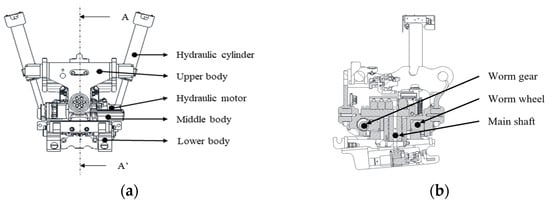
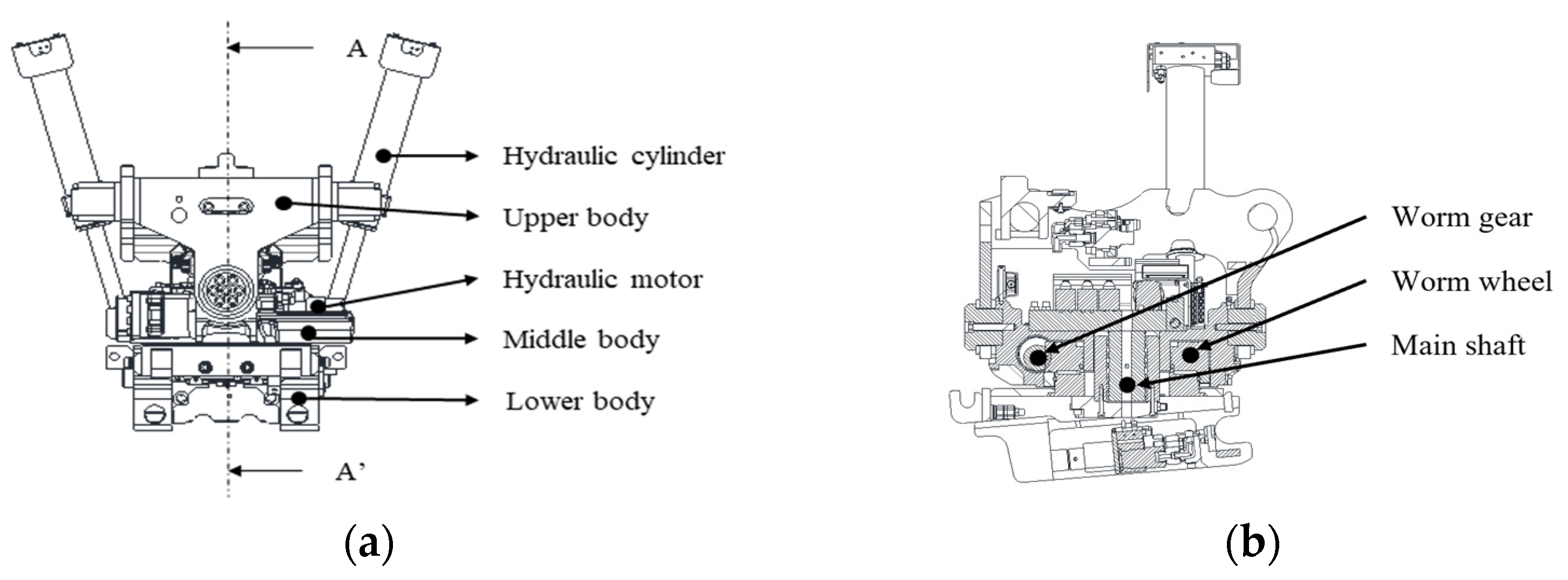
The target system was a 14-ton-class hydraulic excavator equipped with a tilt-rotator between the arm and bucket. Table 1 summarizes the equipment specifications used to define the mechanical and excavation conditions. Figure 2 shows the attachment assembly and its principal load-transfer components. Two hydraulic cylinders connect the upper and middle bodies and generate the tilting motion. A hydraulic motor and worm-drive mechanism rotate the lower body. The attachment provides a tilt range of ±45° and continuous rotation. The motion database used the operating domain of 0–45° tilt and 0–90° rotation defined in Section 2.3. The upper body transfers the arm-side load to the tilting mechanism and was therefore modeled as the flexible component. The middle body, lower body, bucket, and excavator links were modeled as rigid or equivalently simplified bodies.

Table 1. Specifications of the excavator and tilt-rotator.

System	Parameter	Value
Excavator	Class	14 ton
	Maximum bucket payload	600 kg
Tilt-rotator	Mass	360 kg
	Maximum tilt angle	±45°
	Rotation angle	±360°

Figure 2. Tilt-rotator system used in the MBD model: (a) attachment assembly and (b) internal configuration of the principal load-transfer components.

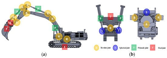
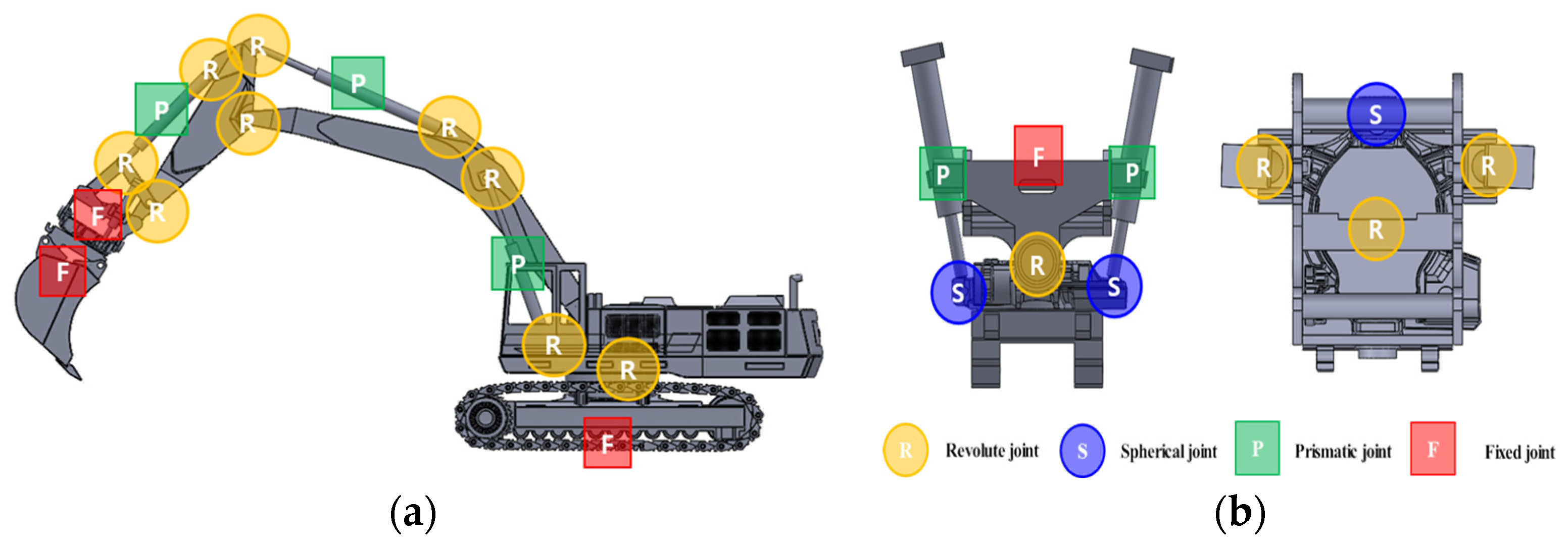
The joint definitions of the MBD model are shown in Figure 3. Revolute, prismatic, and fixed joints were used for the excavator. The tilt-rotator additionally required spherical joints at the cylinder connections to prevent an overconstrained model. These joints reproduced the swing motion of the upper structure, the hydraulic-cylinder motions of the boom and arm, the cylinder-driven tilt motion, and the continuous rotation of the lower attachment body.

Figure 3. Joint definitions used in the multibody dynamics model: (a) revolute, prismatic, and fixed joints of the excavator and (b) revolute, spherical, prismatic, and fixed joints of the tilt-rotator (adapted from Kim et al. [16]).

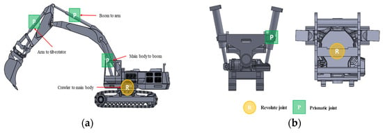
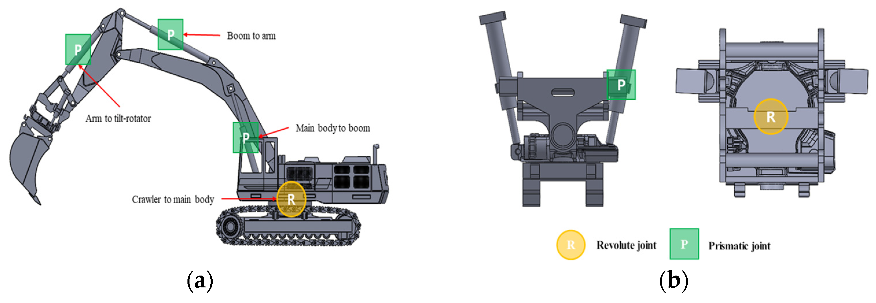
Figure 4 identifies the active joints used to prescribe the two reference operating modes. The excavator motion was generated by the main-body swing joint and by the prismatic inputs of the boom, arm, and arm-to-tilt-rotator connections. The tilt motion was generated by the two prismatic joints between the upper and middle tilt-rotator bodies, whereas the rotation motion was generated by the revolute joint between the middle and lower bodies. Step functions were applied to the prescribed joint inputs to avoid impulsive changes at the beginning and end of the 8 s simulation.

Figure 4. Active joint inputs used to reproduce the reference operating modes: (a) excavator swing and hydraulic-cylinder joints and (b) tilt-rotator tilt and rotation joints (adapted from Kim et al. [16]).

Table 2 lists the input amplitudes used for the two operating modes. Both modes used the same boom, arm, and bucket-positioning motions. Mode 1 retained the neutral tilt and rotation positions. Mode 2 added a 200 mm tilt-cylinder input and a 90° rotation input. Thus, the comparison isolated the additional tilt-rotator motions while maintaining the same base excavator motion.

Table 2. Motion-joint input conditions for the two reference operating modes [16].

Connected Bodies	Joint Type	Mode 1	Mode 2
Crawler–main body	Revolute	0°	0°
Main body–boom	Prismatic	300 mm	300 mm
Boom–arm	Prismatic	600 mm	600 mm
Arm–tilt-rotator	Prismatic	900 mm	900 mm
Tilt-rotator upper–middle bodies	Prismatic	0 mm	200 mm
Tilt-rotator middle–lower bodies	Revolute	0°	90°

The joint topology in Figure 3 and the prescribed active inputs in Figure 4 define the kinematic basis of the MBD model. Section 2.2 specifies the soil-force, moment, and retained-soil mass inputs. The analysis was performed for 8 s with 2000 calculation steps per second. The experimentally correlated model reported in [16] was used as the structural baseline for the expanded operating-motion analysis.

The field vibration test and its two prescribed operating modes were originally reported by Kim et al. [16] and are presented in Figure 5 to establish the experimentally validated basis for the present investigation. The sand surface was prepared before each test to reduce the influence of local surface irregularities. Mode 1 used the neutral bucket posture, whereas Mode 2 used prescribed tilt and rotation motions. Accelerometers were installed on the upper, middle, and lower bodies of the tilt-rotator. The upper body produced the largest measured response and was therefore identified as the critical component for flexible-body representation. The present contribution begins after this inherited validation stage, with the expanded soil-force model, operating-condition database, learning environments, and structural-load-aware policy formulation.

Figure 5. Field vibration test used for MBD model correlation: (a) Mode 1 with the neutral attachment posture and (b) Mode 2 with tilt-rotator operation (adapted from Kim et al. [16]).

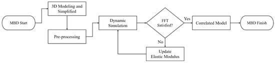
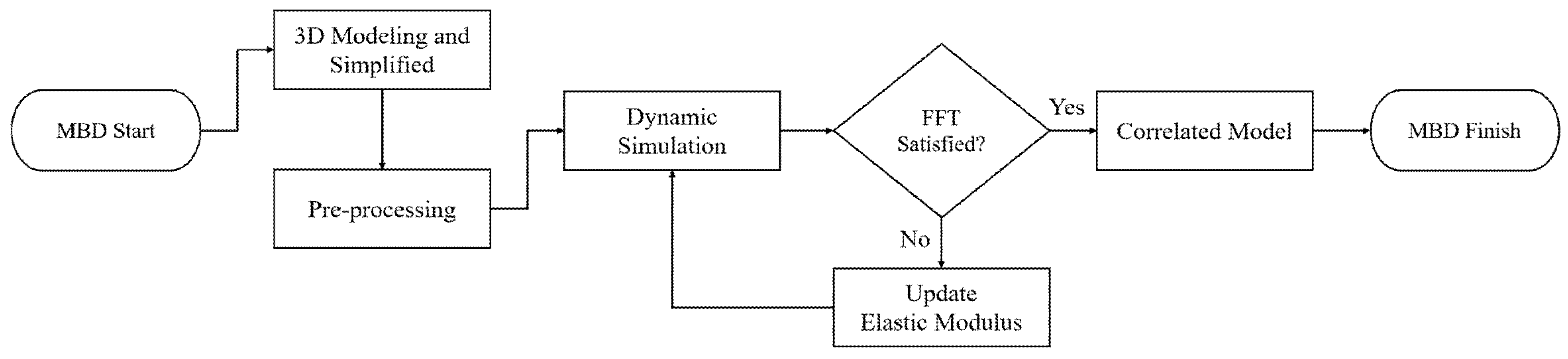
Figure 6 presents the iterative model-correlation workflow. After simplification and preprocessing, the MBD simulation generated acceleration responses that were transformed to the frequency domain using the fast Fourier transform. The dominant simulated frequencies were then compared with the vibration-test peaks. If the agreement criterion was not satisfied, the Young’s modulus E of the flexible upper body was updated and the simulation was repeated. Once the dominant frequencies agreed, the correlated model was accepted for response extraction. This procedure produced a final elastic modulus of 187 GPa, compared with the initial value of 207 GPa.

Figure 6. Iterative MBD-model correlation workflow based on comparison of measured and simulated dominant frequencies (modified from Kim et al. [16]).

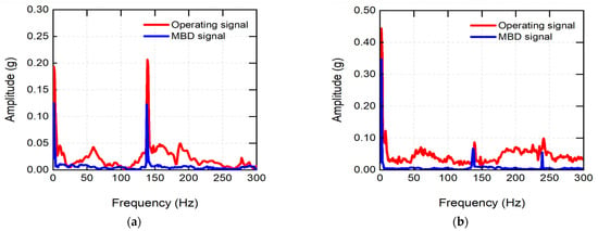
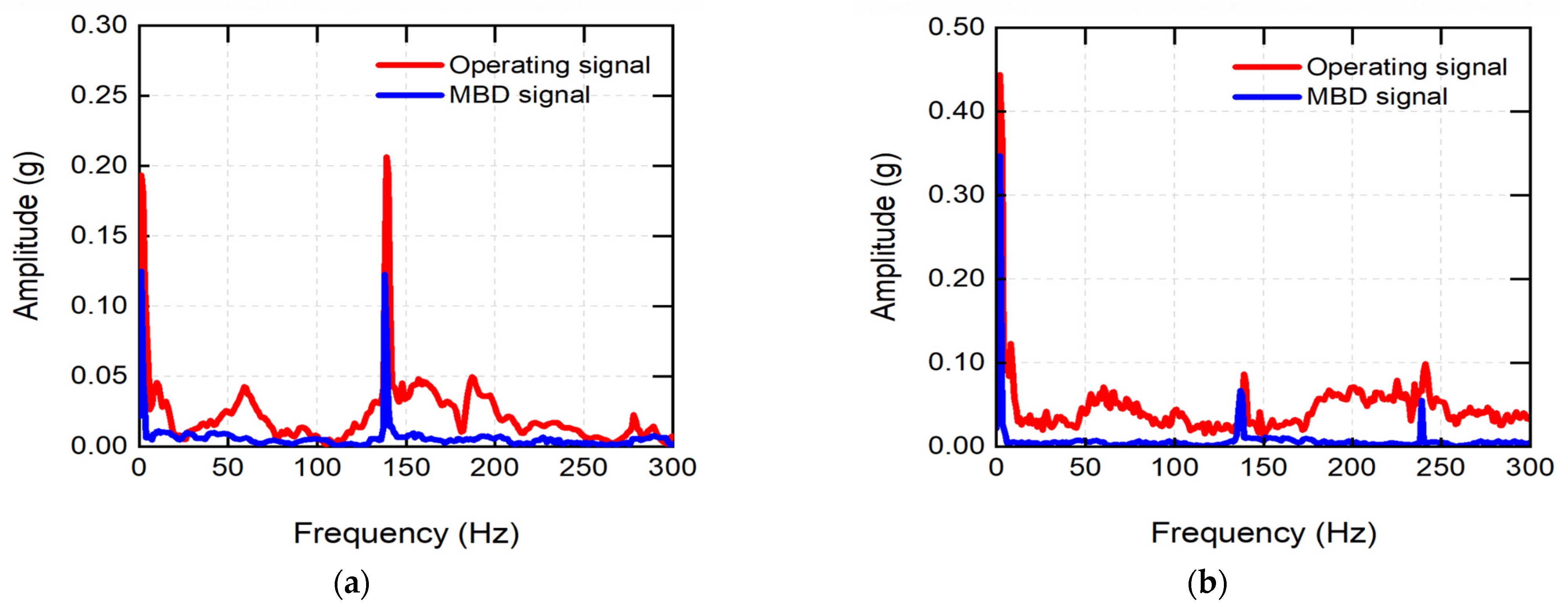
The dominant-frequency comparison was previously reported in [16] and is included here to document the validated mechanical baseline used by the expanded analysis. Table 3 summarizes the paired frequencies, and Figure 7 superimposes the simulated dominant frequencies on the measured spectra. The measured spectra showed peaks at approximately 5.9, 139.3, and 241.3 Hz, and the corresponding simulated frequencies are listed in Table 3. The errors for the five frequency pairs ranged from 1.1% to 8.5%, with a mean value of 4.3%. This agreement supports comparative dynamic-response analysis over the investigated motion set. It does not directly validate stress magnitude or fatigue life.

Table 3. Dominant-frequency correlation between vibration measurements and the MBD model [16].

Tilt-Rotator Mode	Experimental	MBD	Error (%)
	Frequency (Hz)
Mode 1	5.9	5.6	5.1
	139.3	135.9	2.4
Mode 2	5.9	5.4	8.5
	139.3	132.9	4.6
	241.3	238.6	1.1
Mean value (%)			4.3

Figure 7. Frequency-response comparison between the vibration test and the correlated multibody dynamics model: (a) Mode 1 and (b) Mode 2 (adapted from Kim et al. [16]).

2.2. Analytical Soil-Bucket Loads and MBD Application

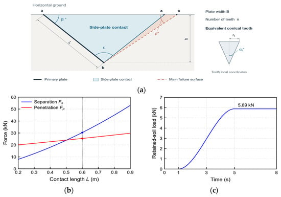
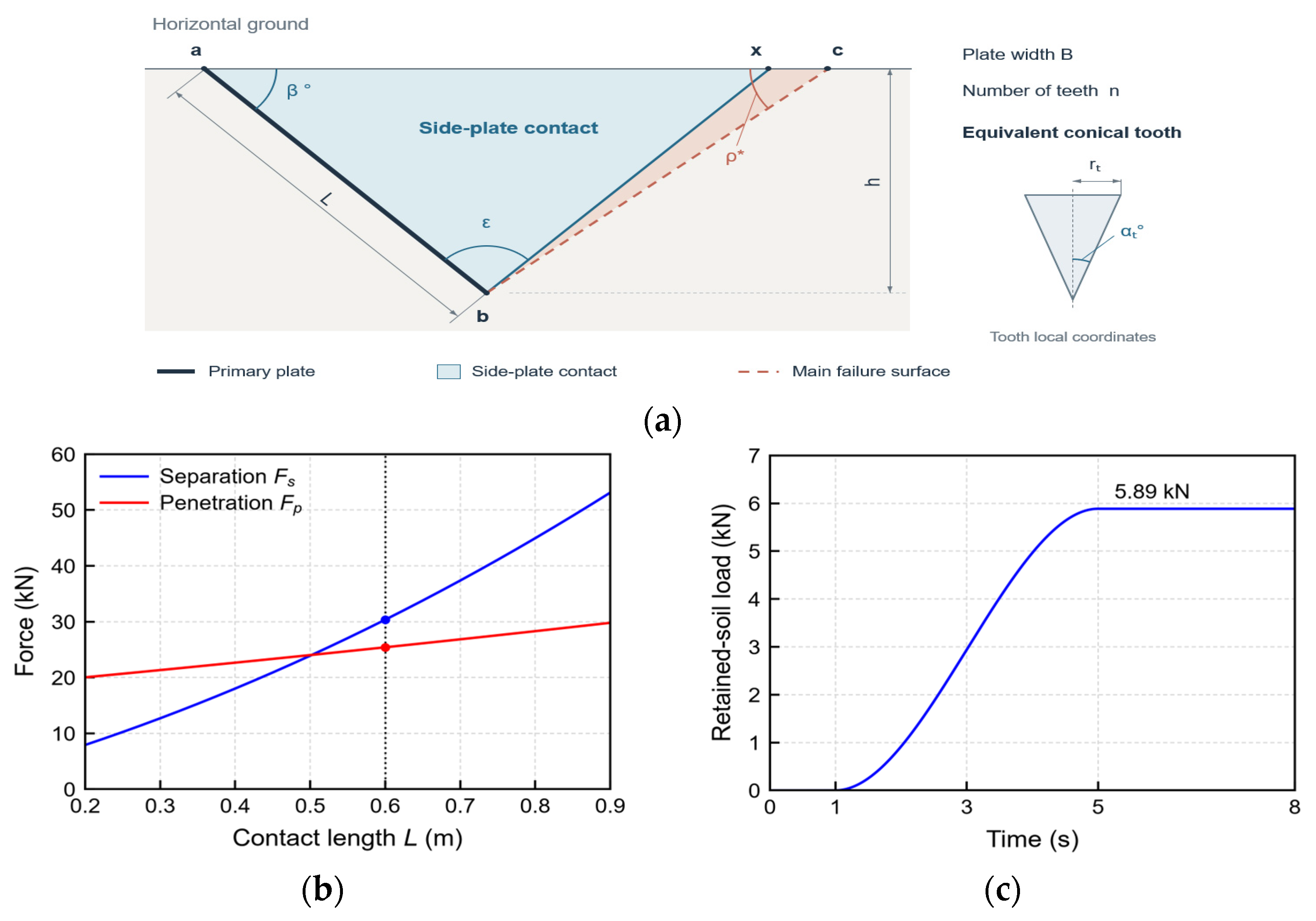
Nominal separation and penetration loads define independent analytical cases [23,24]. Table 4 lists the inputs and loads for Figure 8a. Results are calculated using unrounded values and reported to three significant figures.

Table 4. Nominal parameters and calculated reference loads.

Parameter	Symbol	Value	Unit
Cohesion	c	20	kPa
Adhesion	ca	10	kPa
Soil unit weight	γ	19	kN/m3
Friction angle	φs	27.5	°
Interface friction	δ	20	°
Young’s modulus	Es	20	MPa
Poisson’s ratio	ν	0.25	–
Dilation angle	ψ	0	°
Plate width	B	0.95	m
Contact length	L	0.60	m
Plate angle	β	45	°
Side-plate angle	ε	90	°
Number of teeth	n	5	–
Tooth radius	rt	0.030	m
Tooth half-angle	αt	20	°
Maximum mass	md,max	600	kg
Normal force	Ns	26.2	kN
Tangential force	Ts	15.3	kN
Separation force	Fs	30.4	kN
Sliding resistance	Rps	6.34	kN
Tooth resistance	Rpt	19.1	kN
Penetration force	Fp	25.4	kN
Cavity pressure	p∞	661	kPa
Maximum weight	Fd,max	5.89	kN

Figure 8. Analytical loading: (a) soil-bucket geometry, (b) separation and penetration forces, and (c) retained-soil load history.

The plate reaction R_s is minimized over 0 < ρ ≤ π − β − ε [23]. With normal component N_s = R_s cos δ and tangential component T_s = R_s sin δ + c_a BL, the separation resultant is

$$F_{\mathrm{s}}=\sqrt{{N_{\mathrm{s}}}^2+{T_{\mathrm{s}}}^2}$$

(1)

Plate sliding resistance R_ps and conical-tooth resistance R_pt follow the analytical penetration model [23]. Horizontal ground, zero pore pressure, and tooth axes parallel to the plate are assumed. The limiting pressure p_∞ follows spherical cavity expansion in an isotropic, infinite medium, using the mean geostatic stress at the cutting edge as the initial pressure [24]. The penetration force is

F_p = R_ps + R_pt

(2)

The retained-soil mass m_d(t) of the bucket-CG dummy is zero through 1 s, increases via a cubic STEP function to m_d,max at 5 s, and remains constant until 8 s. Soil resistance follows the same normalized STEP function. With gravitational acceleration g of 9.81 m/s², its weight is

F_d(t) = m_d(t)g

(3)

No additional weight force is applied, and momentum exchange during filling is neglected.

In the bucket frame, separation acts at plate centroid P with −T_s along penetration and N_s along the compressive plate normal. Penetration acts opposite the plate-tangential penetration direction through R_ps at P and R_pt at tooth-row centroid T. After transformation to the global frame, the vector sum of the forces and the sum of their moments about bucket CG C are applied to the fixed dummy. Lever arms are measured from C in the existing geometry using consistent units. Prescribed motions remain unchanged.

The fixed reference geometry and plate-center resultant are idealizations. Ground-surface effects, tooth interaction, and retained-soil redistribution are not resolved. The common STEP profile is prescribed rather than derived from the filling process. These loads provide nominal structural comparisons, and excavation-force histories remain unvalidated.

2.3. Operating-Motion Design and Stress Database

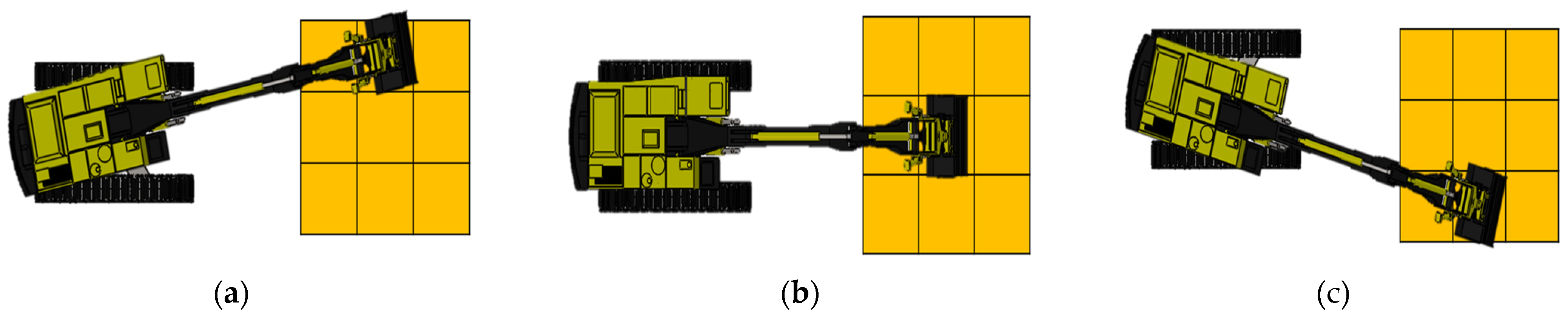
The attachment operating domain was defined by a two-factor, five-level full-factorial design, denoted L₂₅(5²), rather than by a reduced fractional design. The tilt levels were 0°, 11.25°, 22.5°, 33.75°, and 45°, whereas the rotation levels were 0°, 22.5°, 45°, 67.5°, and 90°. The design comprises all 25 tilt-rotation combinations. Each configuration was combined with the nine relative bucket positions distributed among the left-side, front, and right-side excavation directions shown in Figure 9. The resulting database therefore contained 5 × 5 × 9 = 225 candidate motions.

Figure 9. Representative operating directions used to define the nine relative excavation paths: (a) left-side, (b) front, and (c) right-side excavation.

N_cand = N_tilt × N_rot × N_pos = 5 × 5 × 9 = 225

(4)

Here, N_cand denotes the total number of candidate operating motions, while N_tilt, N_rot, and N_pos denote the numbers of discrete tilt levels, rotation levels, and relative excavation positions, respectively.

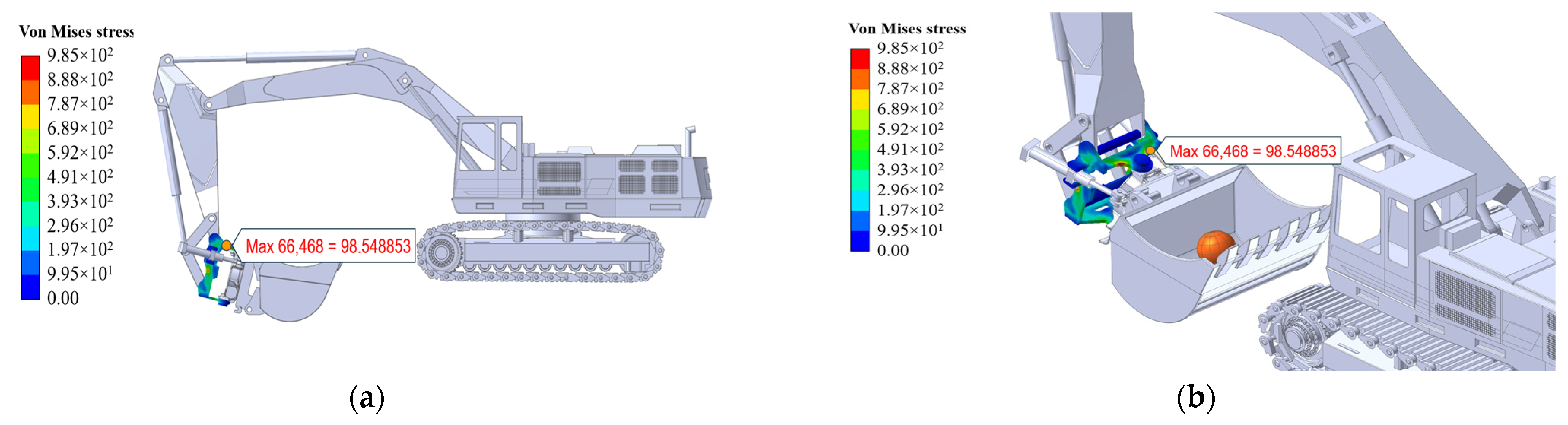
The upper body was selected as the representative flexible component because it is the arm-side load-entry structure of the tilt-rotator, transfers excavation forces and moments into the tilt mechanism, and exhibited the largest measured vibration response in the preceding correlation tests [16]. Figure 10a,b identifies this component in the complete excavator and shows its finite-element representation. The remaining attachment components and excavator links were treated as rigid or equivalently simplified bodies. This selective flexible-body formulation retained local deformation and stress recovery in the critical load-transfer component without imposing the computational cost of a fully flexible excavator model.

Figure 10. Representative dynamic-stress fields in the flexible upper body: (a) location of the critical load-transfer component in the complete 6-DOF excavator model and (b) detailed stress distribution in the tilt-rotator assembly [16].

The operational-admissibility filter was defined before the stress comparison. A candidate motion was classified as redundant when the target could be reached and excavated using the neutral attachment posture, no geometric or obstacle constraint required attachment reorientation, and tilting or rotating provided no additional access to the soil cell. Under these conditions, actuating the tilt or rotation axis would require an unnecessary posture change and additional operating time without improving task completion. The filter therefore excluded 78 operationally unnecessary motions and retained 147 of the 225 candidates. Importantly, this was an operational-efficiency screen rather than a stress-based removal of unfavorable results. The candidate database was generated as the Cartesian product of the 25 tilt-rotation configurations in Table 5 and the nine relative excavation positions in Figure 9. Each candidate record contained the configuration case, tilt angle, rotation angle, relative position, operational-eligibility decision, and, for retained motions, the maximum dynamic stress of the flexible upper body.

Table 5. L₂₅(5²) full-factorial design of the tilt and rotation angles. Entries are configuration case numbers.

	Rotation Angle (°)	0	22.5	45	67.5	90
Tilt Angle (°)
0		1	2	3	4	5
11.25		6	7	8	9	10
22.5		11	12	13	14	15
33.75		16	17	18	19	20
45		21	22	23	24	25

The complete eligibility and stress pattern, including the 78 excluded candidates, is presented in Section 4.1, while Table 6 reports the number and stress range of the 147 retained motions for each relative path. These main-text elements jointly document the database construction, exclusion outcome, and structural-response range.

Table 6. Dynamic-stress distribution of the 147 retained motions by relative excavation path.

Path	Retained Cases	Minimum (MPa)	Mean (MPa)	Maximum (MPa)
1	24	103.8	126.5	146.0
2	24	106.7	124.6	149.0
3	24	102.9	126.4	148.6
4	1	100.6	100.6	100.6
5	1	98.5	98.5	98.5
6	1	102.1	102.1	102.1
7	24	104.1	123.1	149.0
8	24	105.6	123.3	144.1
9	24	103.4	124.8	146.8

3. Topology-Aware Structural-Load-Aware Work-Path Planning

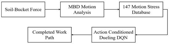
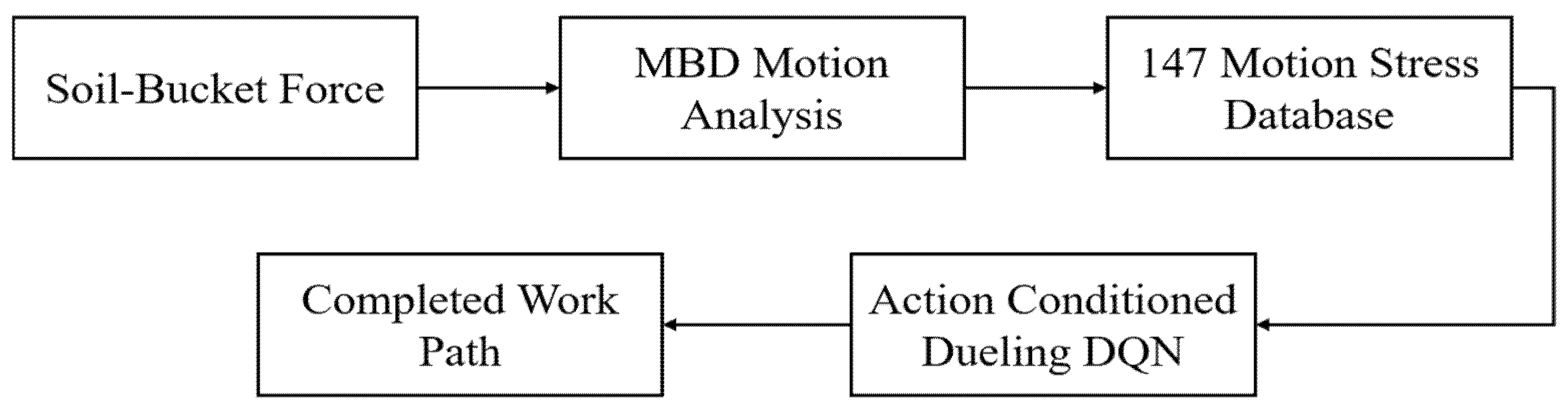
Figure 11 summarizes the analysis and planning procedure. Section 2.2 defines independent nominal separation and penetration cases with a prescribed ramp for soil resistance and retained-soil mass. Soil forces are transformed into the global frame and transferred with their moments to the fixed bucket-CG dummy, whose mass is subject to gravity. The MBD stress database assigns a structural-response value to each eligible excavation action. The DQN then selects movement, turning, and excavation actions until all accessible soil cells are removed.

Figure 11. Information flow from nominal soil-bucket loading and multibody dynamics analysis to the structural-load-aware work-path policy.

3.1. Learning Environments and Excavation Topology

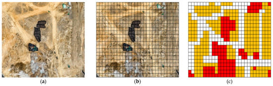
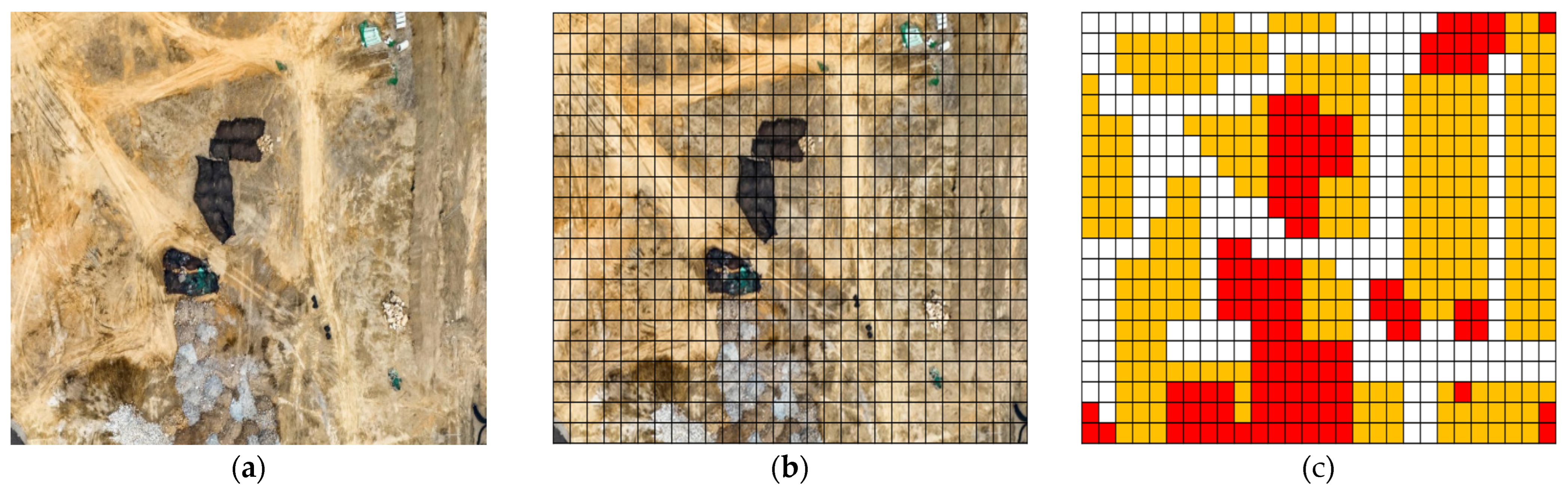
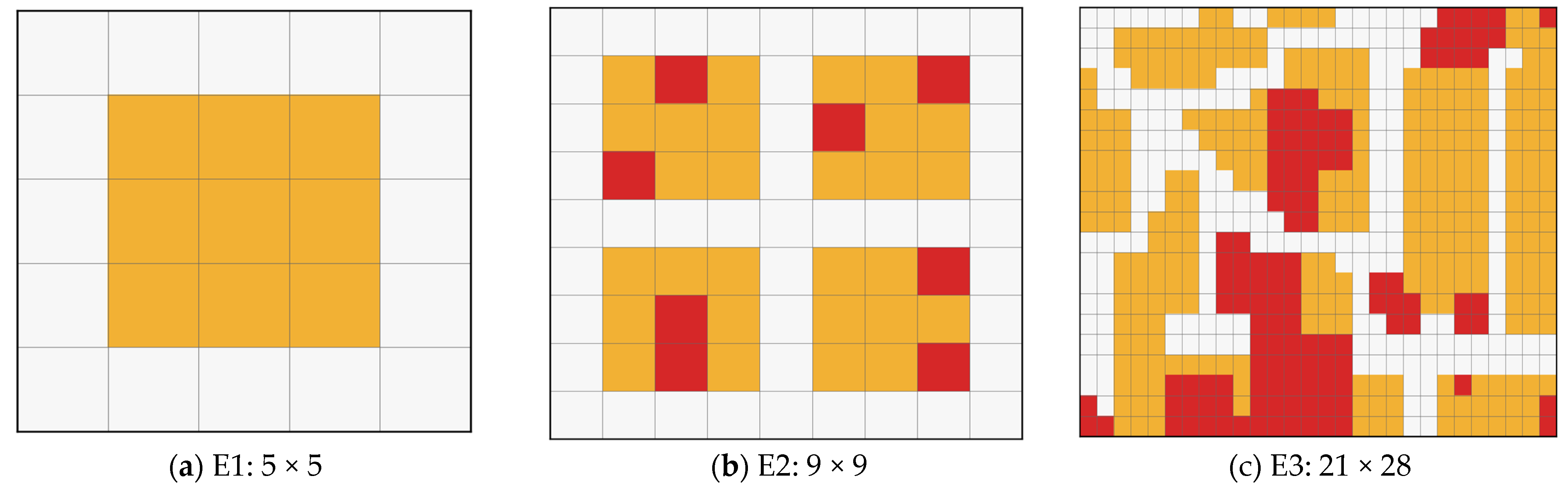
Three discrete numerical environments were used. E1 was a 5 × 5 controlled environment with 9 soil cells. E2 was a 9 × 9 environment with 28 soil cells and 8 obstacles. E3 was constructed from the actual construction site shown in Figure 12a. A regular grid was superimposed on the site image (Figure 12b), and each cell was classified as a carrier path, soil region, or obstacle region (Figure 12c).

Figure 12. Construction of the site-derived E3 environment: (a) actual construction-site image, (b) regular grid superimposed on the site, and (c) source categorical representation used to digitize soil, obstacle, and carrier-path cells [16]. In panel (c), yellow, red, and white cells denote soil, obstacles, and carrier paths, respectively. The source color map was digitized and reconciled against the final numerical input file. The horizontal cell size was set to approximately 0.6 m × 0.6 m using the bucket-capacity scaling of the source study. The verified E3 input contained 21 rows, 28 columns, 280 soil cells, 188 carrier-path cells, and 120 obstacle cells. These counts refer to the final input file rather than to a historical printed total.

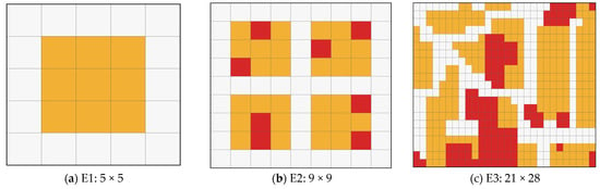
Figure 13 compares the three numerical environments used for learning. The E1 and E2 grids provide controlled cases with different levels of obstacle and route complexity. E3 preserves the irregular spatial distribution derived from the actual site. It is described as a site-derived numerical environment because the learned policy was evaluated only in simulation and was not deployed on the actual excavator. The numerical characteristics and the role of each environment are listed in Table 7.

Figure 13. Numerical environments used for learning: (a) E1, (b) obstacle-containing E2, and (c) site-derived E3. Yellow denotes soil, red denotes obstacles, and white denotes carrier paths.

Table 7. Characteristics and roles of the three numerical environments.

Environment	Grid	Path Cells	Soil Cells	Obstacles	Role
E1	5 × 5	16	9	0	Controlled small case
E2	9 × 9	45	28	8	Obstacle-containing comparison
E3	21 × 28	188	280	120	Site-derived scalability case

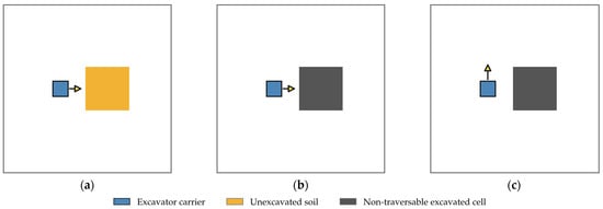
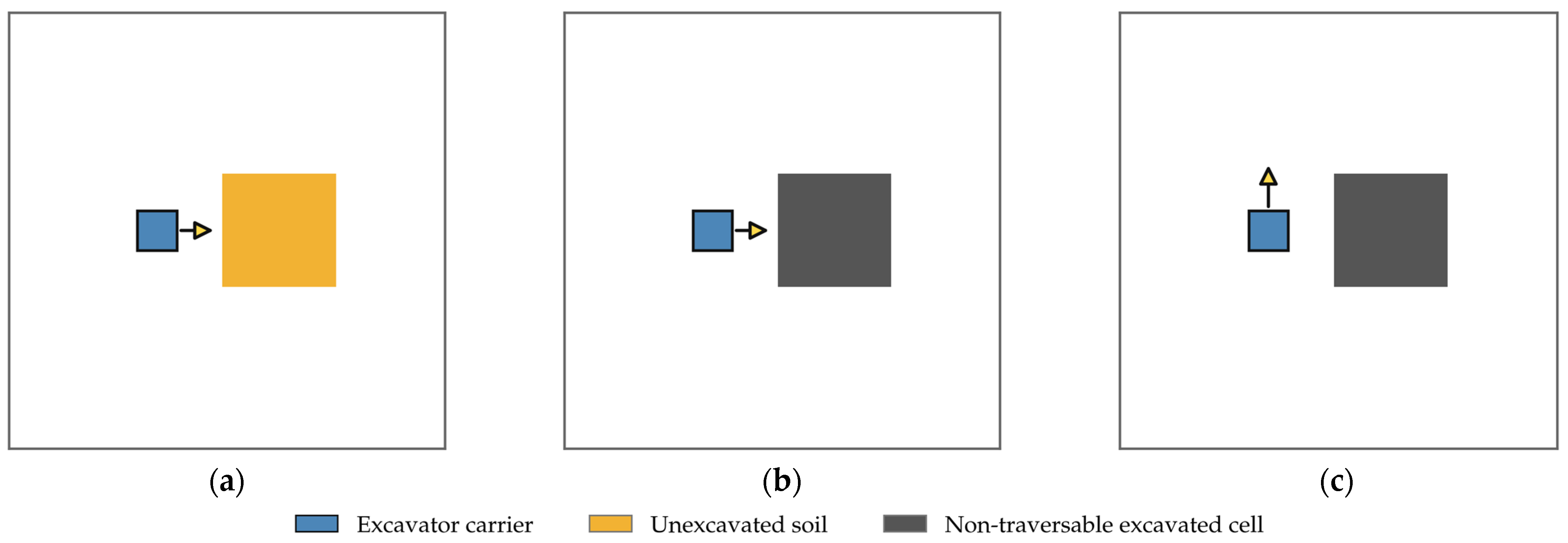
Figure 14 is a state-transition schematic, not a performance result. It defines the topological rule used by the Markov decision process [25,26] after a successful excavation. The removed soil cell changes from traversable work material to a non-traversable hole rather than to a carrier path, thereby preventing the excavator from traveling across excavated ground. Because this update can otherwise make a remaining soil cell unreachable when heading changes occur only during translation, two in-place turning actions were added.

Figure 14. Schematic definition of the topology-aware state transition used in the learning environment: (a) the carrier faces an unexcavated soil cell, (b) successful excavation converts that cell into a non-traversable hole, and (c) an in-place turn changes the carrier heading while preserving the carrier position. The yellow arrow indicates the current carrier heading.

In Figure 14, the blue square denotes the carrier, the high-contrast yellow arrow denotes its heading, the yellow cell denotes unexcavated soil, and the dark-gray cell denotes the hole created after excavation. A left or right turn changes only the heading and preserves the carrier position.

3.2. Agent Profiles, State, and Action Space

The three agent definitions are summarized in Table 8. Agent 1 represented a conventional excavator. Some off-axis soil cells required two excavation passes, whereas cells aligned with the front path could be removed in one pass. Agent 2 represented the six-degree-of-freedom (6-DOF) machine without stress information or posture-repeat control. Agent 3 used the same kinematic capability and added normalized stress information and a conditional repeat-posture mask. Reuse of the immediately preceding posture was prohibited only when another productive posture was available. Otherwise, the mask was relaxed to preserve task feasibility.

Table 8. Agent definitions used in the numerical study.

Agent	Machine	Stress Feature and Penalty	Conditional Posture Mask
Agent 1	Conventional excavator	No	No
Agent 2 (S0R0)	6-DOF excavator	No	No
Agent 3 (S1R1)	6-DOF excavator	Yes	Yes

The 147 eligible stress values were normalized as follows:

$$z_{\sigma }={\displaystyle \frac{\sigma -{\sigma }_{\min }}{{\sigma }_{\max }-{\sigma }_{\min }}}$$

(5)

Here, z_σ denotes the dimensionless normalized dynamic-stress index assigned to a candidate excavation action. The variable σ is the maximum dynamic stress predicted by the MBD model for that action, whereas σ_min = 98.5 MPa and σ_max = 149.0 MPa are the minimum and maximum values among the 147 retained motions, respectively. Consequently, 0 ≤ z_σ ≤ 1, where 0 and 1 represent the least and most structurally demanding retained motions, respectively.

For Agent 3, z_σ was used both as an action feature and in the stress-dependent reward term. It represents a relative structural-load preference and not an allowable-stress ratio or damage criterion. The action space contained four translations, two in-place turns, and 25 × 9 = 225 excavation actions. Hence, the total action dimension was 231. Invalid movements, obstacles, excavated holes, out-of-grid targets, and ineligible configuration–path pairs were removed by a state-dependent mask.

The global state was represented by 12 semantic channels defined over an H × W grid, where H and W denote the grid height and width, respectively. The channels were as follows: (1) carrier-path indicator; (2) unexcavated-soil indicator; (3) obstacle indicator; (4) one-hot carrier-position plane; (5) the remaining-soil ratio repeated over the grid; (6–9) four one-hot heading planes for north, south, west, and east; (10) cellwise excavation progress normalized by the two-pass maximum; (11) a spatially repeated stress-signal flag, equal to 1 only for Agent 3; and (12) the previous tilt–rotation case index normalized by 25, with −1 used before any excavation posture had been selected. A five-channel 7 × 7 egocentric local window was centered on the excavator and rotated so that the current heading pointed upward. This local representation contained the path, soil, obstacle, excavation-progress, and in-grid planes and reduced dependence on absolute position. Dynamic action features described the target cell, excavation progress, local soil and obstacle ratios after movement or turning, and the distance from a prospective movement cell to the nearest viable work position. Shortest-path distances between fixed carrier-path cells were precomputed by breadth-first search.

3.3. Reward Function

A successful excavation action received a base reward divided by the number of passes required for that cell. Completing the kth soil cell yielded an additional cumulative progress bonus. For large environments, the cumulative coefficient was scaled relative to the 28-cell E2 reference to prevent the state value from increasing solely with map size:

$$r_{\mathrm{dig},k}={\displaystyle \frac{30}{q_k}}+5\mathit{min}\left(1,{\displaystyle \frac{28}{N_{\mathrm{soil}}}}\right)(k-1)$$

(6)

Here, r_dig,k denotes the unscaled positive reward assigned to the kth successful excavation. The index k is the ordinal index of successfully excavated soil cells, q_k is the number of passes required for the corresponding cell, and N_soil is the total number of soil cells in the environment. The first term rewards successful removal, whereas the second term provides a cumulative progress bonus scaled relative to the 28-cell E2 reference. A movement or in-place turn received a movement penalty of −1 and a time penalty of −0.5 per second. A soil excavation required 15 s, a movement or turn required 2 s, and an obstacle excavation incurred a penalty of −100. For Agent 3, the successful-dig reward was reduced according to normalized stress as follows:

r_σ,k = −0.10 r_dig,kz_σ,k

(7)

Here, r_σ,k denotes the stress-dependent reward adjustment applied to the kth successful excavation. The term r_dig,k is the positive excavation reward from Equation (6), and z_σ,k is the normalized dynamic-stress index of the selected excavation action. The negative sign therefore imposes a larger reduction for a more structurally demanding action. The multiplier 0.10 bounds this reduction to 10% of the corresponding positive excavation reward. The term was applied only to successful excavation, and all rewards were multiplied by 0.1 before optimization. It is a preference-shaping mechanism rather than a stress limit or damage criterion.

The value 0.10 was fixed before the additional experiments so that task completion remains the dominant objective while predicted stress decides among equally productive postures. For the additional study, the multiplier is denoted by α and was varied over 0, 0.05, 0.10, and 0.20 while retaining the S1R1 inputs and mask. The value is a trade-off weight between task efficiency and predicted structural load rather than a calibrated or optimal value, and the coefficient study reports the observed trade-off within the tested range.

3.4. Action-Conditioned Dueling DQN

The action-value learning framework combines model-free Q-learning [27] with the DQN approach, which uses neural function approximation, experience replay, and a target network [28]. The global state passed through fully connected layers of 128, 128, and 64 units. The local 5 × 7 × 7 window passed through a 128–64 encoder. Static and dynamic action features were embedded into 64 units and fused with the state representation. A Dueling head separated the scalar state value from the action-specific advantage [29]:

$$Q(s,a)=V(s)+A(s,a)-{\displaystyle \frac{1}{|\mathcal{A}(s)|}}\sum _{{\mathit{a}}^{\prime }\in \mathcal{A}\left(s\right)}A(s,{\mathit{a}}^{\prime })$$

(8)

Here, Q(s, a) is the action value, V(s) is the state value, A(s, a) is the action advantage, and 𝒜(s) is the nonempty set of valid actions. The summation and its normalization both use 𝒜(s), so masked actions do not affect the advantage mean. The baseline target uses the ordinary DQN maximum. Three-step returns are accumulated with an effective horizon n of one to three transitions at episode boundaries:

$$y_t={\displaystyle \sum _{i=0}^{n-1}}{\gamma }^i{r}_{t+i}+{\gamma }^n(1-d_{t+n}){\mathit{max}}_{{\mathit{a}}^{\prime }\in \mathcal{A}\left(s_{t+n}\right)}{Q}^{-}(s_{t+n},{\mathit{a}}^{\prime }),n\in \{1,2,3\}$$

(9)

Here, y_t is the temporal-difference target; n ∈ {1, 2, 3} is the number of accumulated transitions, that is, the effective horizon; r_t+i is the learning reward after the global 0.1 scaling; and γ = 0.95 is the discount factor. The terminal indicator d_t+n equals 1 if the accumulated return reaches task completion or a state with no valid action, in which case the bootstrap term is zero. Step-limit and stall cutoffs are truncations: d_t+n remains zero and bootstrapping uses the final observed state. Q⁻ is the target network, and the maximum is restricted to the valid actions 𝒜(s_t+n) at that state.

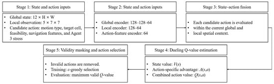
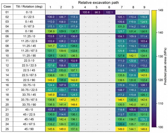
Figure 15 organizes the action-conditioned Dueling DQN into five sequential stages. First, the complete 12 × H × W state represents environment-wide progress and topology, the heading-aligned 5 × 7 × 7 observation represents the carrier’s immediate neighbourhood, and the candidate-action descriptor identifies the proposed movement, turn, or excavation together with its target, navigation, feasibility, and Agent 3 stress information. Second, separate encoders transform these three inputs into compact feature vectors. Third, the encoded state and action vectors are fused so that every candidate is evaluated in the current spatial context. Fourth, the Dueling head estimates the state value V(s) and the action-specific advantage A(s,a), which are combined to obtain Q(s,a). Finally, the state-dependent validity mask removes obstacle excavation, movement into holes, out-of-grid actions, and ineligible configuration-path pairs before action selection. Training uses epsilon-greedy selection among valid actions, whereas deterministic evaluation selects the valid action with the largest Q-value.

Figure 15. Five-stage information flow of the action-conditioned Dueling DQN: state and candidate-action inputs are encoded, fused, evaluated through value and advantage streams, and filtered by the state-dependent validity mask before action selection.

Smooth L₁ loss, a Huber-type piecewise loss, was used to quantify the error between the predicted Q-values and the temporal-difference targets. Its quadratic response to small errors and linear response to large errors reduce the influence of occasional large temporal-difference errors compared with a purely quadratic loss. Adam [30] was used to minimize this loss. The replay capacity was 100,000 transitions, the minibatch size was 32, the learning rate was 5 × 10⁻⁴, and the discount factor was 0.95. The target network was updated every 1000 optimizer steps, and the gradient norm was limited to 10. Exploration decreased linearly from 0.90 to 0.05 after environment-dependent pretraining. To increase the number of late-task states, 50% of training episodes started from a randomly generated valid intermediate state. Every deterministic evaluation started from the original state. When a random action was required, 50% of movement selections were guided toward a precomputed viable work position. Table 9 lists the network configuration, fixed learning parameters, and the environment-dependent schedules. The architecture and optimization settings were identical across the three profiles. Agent-specific differences were limited to the machine and action definitions, stress information, and conditional posture-repeat mask.

Table 9. DQN configuration and training parameters used for the three excavator agents. Section 3.6 specifies the additional fixed-budget study.

Configuration or Parameter	Value	Applicability
Agent profile	A1/S0R0/S1R1	Agents 1/2/3
Machine model	Conventional/6-DOF/6-DOF excavator	Agents 1/2/3
Stress feature and reward term	No/No/Yes	Agents 1/2/3
Conditional posture-repeat mask	No/No/Yes	Agents 1/2/3
Total action dimension	231: 4 translations + 2 turns + 225 excavation actions	All agents; invalid actions masked
Global-state encoder	12 semantic channels over an H × W grid; fully connected 128–128–64	All agents
Egocentric encoder	5 × 7 × 7; fully connected 128–64	All agents
Action-feature embedding	Static and dynamic features → 64	All agents
Q-network/target	Dueling DQN/ordinary DQN maximum	All agents; not Double DQN
Optimizer/loss	Adam/Smooth L1	All agents
Learning rate/discount factor	5 × 10−4/0.95	All agents
Minibatch/replay capacity	32/100,000 transitions	All agents
Learning warm-up/target update	2000 transitions/1000 optimizer steps	All agents
Multi-step return/reward scale	3 steps/0.1	All agents
Gradient-norm limit	10	All agents
Exploration	ε: 0.90 → 0.05, linear	All agents
Randomized starts/guided movement	0.50/0.50	Training only
Independent seed	11	One run per combination
Environment schedule	E1: 3000/3000/200; E2: 10,000/10,000/400; E3: 100,000/100,000/4000	Pretraining actions/evaluation interval/maximum episode actions

A Dueling value-based representation was selected because the present action set is finite and explicitly masked, and the action-conditioned encoder can evaluate each eligible motion descriptor. This is a design choice, not a claim that other learning methods are unsuitable.

3.5. Deterministic Evaluation and Convergence

For the original E1–E3 case studies, evaluation used greedy masked actions with no exploratory sampling. A run was declared converged only when the current exploration rate was no greater than its terminal value, ε_end = 0.05, and the excavation task was completed in all five of the most recent evaluations with a maximum action count no greater than 110% of the minimum count in that window. Let D₅ denote the number of completed evaluations in the five-evaluation window and let ρ₅ denote the ratio of the maximum action count to the minimum action count in that window. The engineering stopping criterion was

C = I[ε ≤ ε_end ∧ D₅ = 5 ∧ ρ₅ ≤ 1.10]

(10)

Here, I[·] denotes the indicator function. For the current evaluation index k, let W_k = {k − 4,…, k}. The binary variable c_j equals 1 when evaluation j completes the entire excavation task and 0 otherwise, while N_j > 0 is its total action count. Accordingly, D₅ is the sum of c_j over W_k, and ρ₅ is the ratio of the maximum to the minimum N_j over the same window. Therefore, C = 1 only when the exploration rate has reached its terminal level, all five evaluations are complete, and their action counts satisfy the 10% stability bound. This criterion was used only as an engineering early-stopping rule and does not constitute statistical or theoretical proof of DQN convergence.

The stored route was selected from the completed deterministic evaluations during training and had the fewest total actions. The storage key did not include stress. Consequently, the stored route is described as the selected minimum-action completed route, not as a structural optimum. Raw episode-wise training-reward and duration curves were not used for cross-agent comparison because epsilon-greedy exploration and randomized intermediate starts deliberately mix trajectories with different initial states. Instead, agent-specific fixed-policy evaluation histories for all three agents in E1 and E2 are presented in Section 4.2, while the corresponding history for E3 Agent 3 is presented in Section 4.3. These deterministic evaluations, together with the fixed network and training parameters in Table 9 and the convergence and selected-route statistics in Table 10 and Table 11, provide the reproducible basis for performance comparison. Every deterministic evaluation began from the original environment state, providing a consistent basis for completion and action-count comparison.

Table 10. Archived selected minimum-action completed routes in E1 and E2 (seed 11). The move count equals the carrier travel length in cell units.

Environment	Agent	Convergence Actions	Route Actions (Move + Turn + Dig)	Virtual Time (s)	Stress Index (MPa)
E1	Agent 1	42,002	15 (3 + 3 + 9)	147	Not used
E1	Agent 2	36,004	12 (2 + 1 + 9)	141	1044.7
E1	Agent 3	36,002	13 (2 + 2 + 9)	143	1088.3
E2	Agent 1	180,024	55 (11 + 8 + 36)	578	Not used
E2	Agent 2	110,021	47 (15 + 4 + 28)	458	3361.8
E2	Agent 3	170,032	44 (10 + 6 + 28)	452	3158.0

Table 11. E3 Agent 3 learning milestones and selected route.

Metric	Value
First deterministic completion	Approximately 0.7 million training actions
Convergence	1,600,084 training actions
Selected route	453 actions
Route composition	154 moves + 19 turns + 280 excavations
Virtual time	4546 s
Cumulative peak-stress index	29,604.4 MPa
Obstacle excavation attempts	0

3.6. Additional Fixed-Budget E2 Study

Seven conditions were trained independently with seeds 11, 22, and 33: S0R0, S1R0, S0R1, and S1R1 at α = 0.10; S1R1 at α = 0.05 and 0.20; and S1R1 at α = 0. In the 2 × 2 comparison, S enables the stress action feature, the stress-enabled observation flag, and the penalty together, and R enables the conditional posture-repeat mask; the α = 0 condition retains the stress inputs and the mask and removes only the penalty, so that the factorial S effect concerns the stress package whereas the α = 0 comparison isolates the penalty. All runs used the same E2 task, architecture, optimizer settings, exploration schedule, and nominal 400,000-action budget, with evaluations every 25,000 actions and no early stopping. The primary endpoint was the greedy policy at the final budget, evaluated from the original state; the secondary endpoint is the first minimum-action completed evaluation in the recorded sequence, and the two are reported separately. Means and sample standard deviations describe the observed runs and do not establish population-level superiority.

4. Results and Discussion

4.1. Configuration-Dependent Dynamic Stress

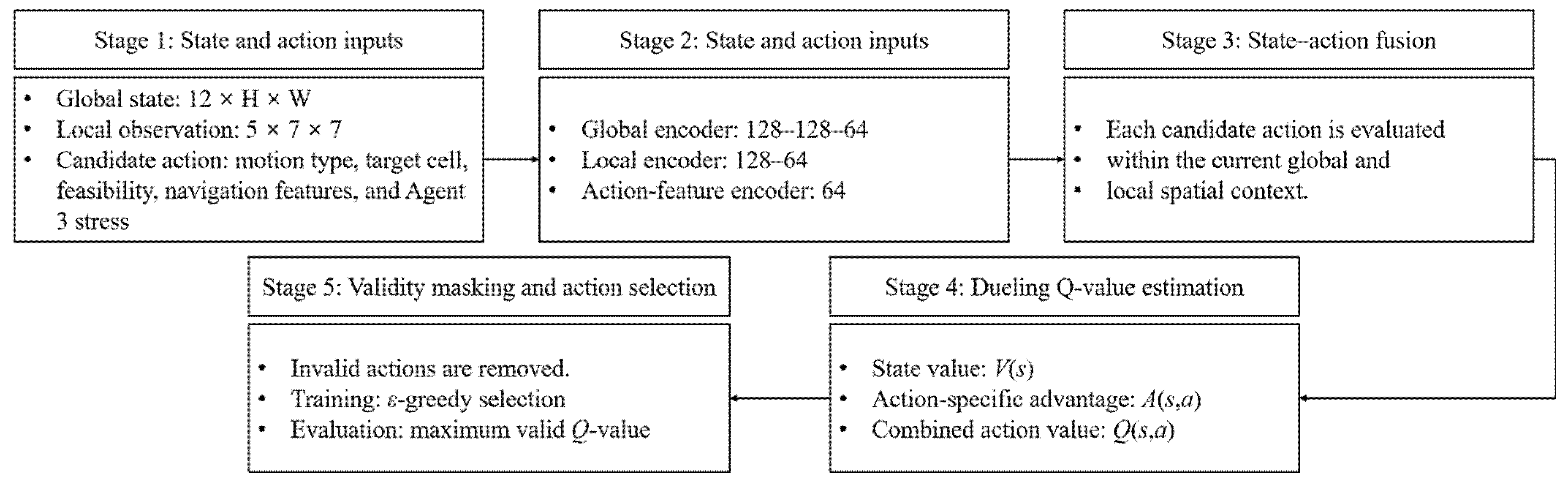
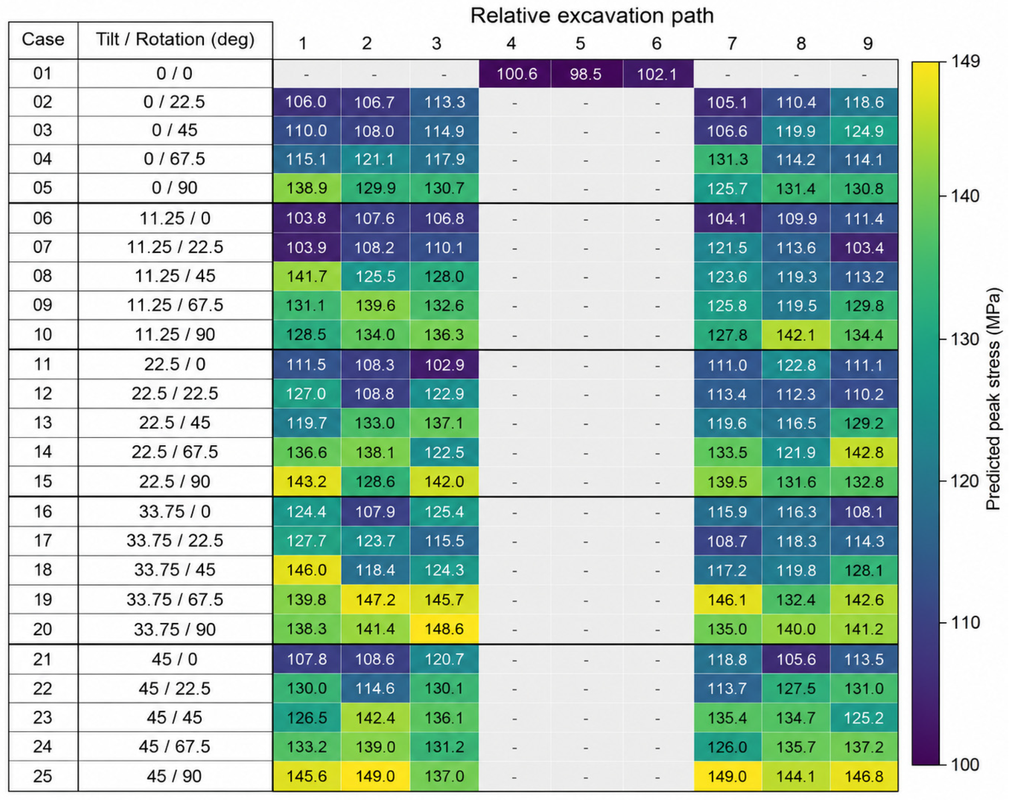
The retained motions produced maximum dynamic stresses ranging from 98.5 to 149.0 MPa. Figure 16 shows the stress assigned to every retained configuration-path pair. Blank cells indicate excluded motions. The overall mean and standard deviation were approximately 124.3 and 13.0 MPa, respectively. The minimum occurred for Case 1 at Path 5, whereas the maximum occurred for Case 25 at Paths 2 and 7. At Path 3, the stress range across eligible configurations was 102.9–148.6 MPa. At Path 7, it was 104.1–149.0 MPa. Thus, changing the attachment configuration altered the peak stress by approximately 45 MPa for the same relative excavation direction. A single excavation-load value cannot represent the expanded operating workspace.

Figure 16. Maximum dynamic stress for the 147 retained configuration-path motions. Blank cells denote motions excluded by the prescribed operating-condition filter.

4.2. Learning and Completion in E1 and E2

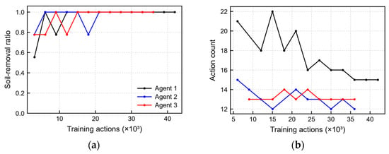
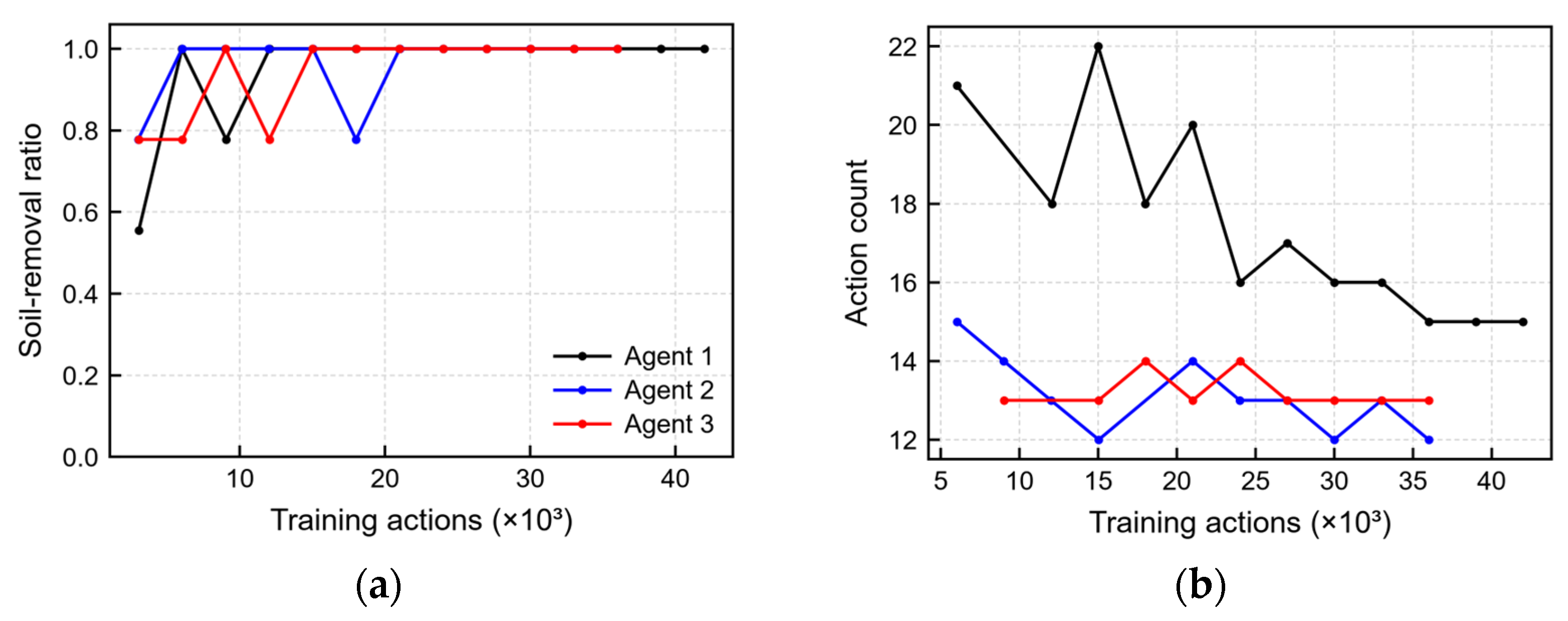
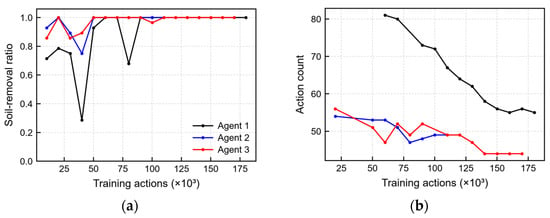
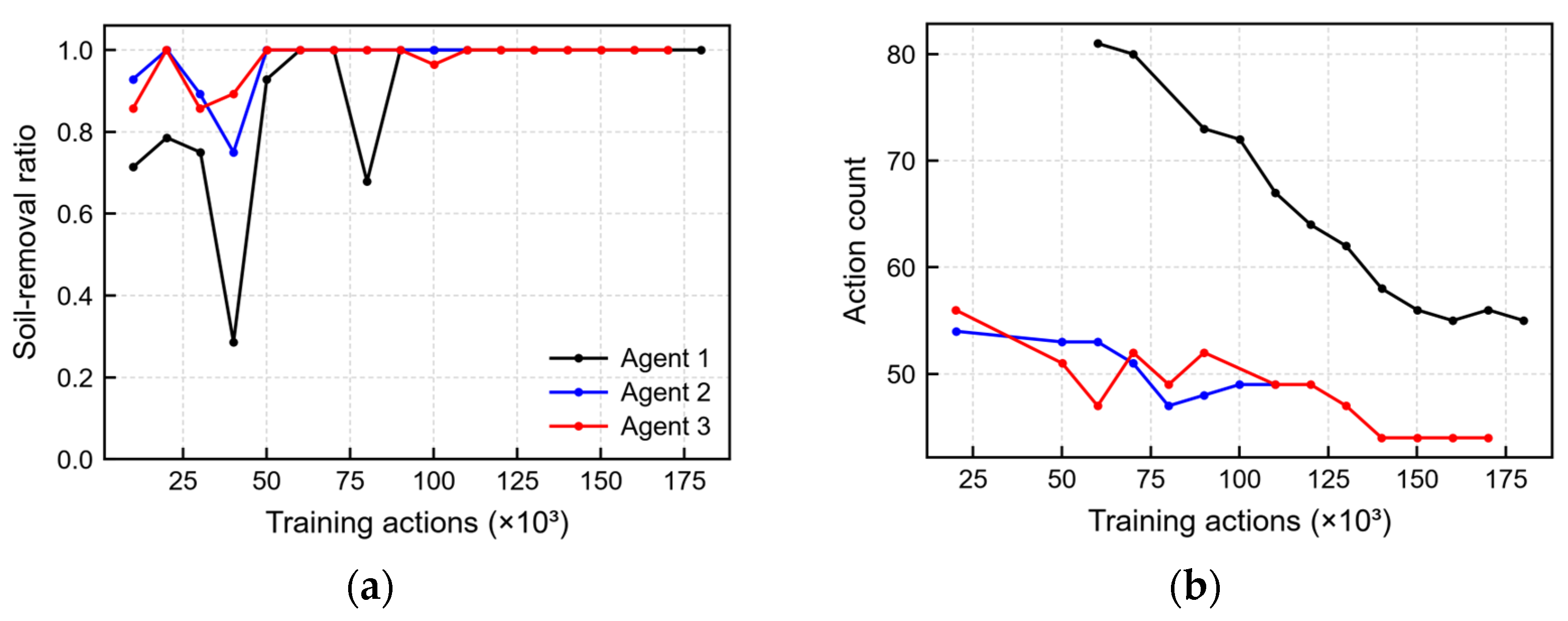
All six E1 and E2 agent-environment combinations satisfied the development convergence criterion. In E1, Agents 1, 2, and 3 converged after 42,002, 36,004, and 36,002 training actions, respectively. The evaluation histories are shown in Figure 17. In E2, the corresponding values were 180,024, 110,021, and 170,032, as shown in Figure 18. The larger training-action count of E2 Agent 3 shows that structural information did not automatically accelerate learning. The final comparison therefore uses the selected completed routes from deterministic evaluation rather than convergence speed alone. Table 10 lists the convergence action count and the selected-route metrics for each E1 and E2 Agent. Agent 1 is reported without a stress index because its action definition does not use the tilt-rotator stress database. For Agents 2 and 3, the reported index is the sum of the event-wise maximum stresses over all successful excavation actions.

Figure 17. Deterministic evaluation history in E1: (a) soil-removal ratio and (b) action count for completed evaluations.

Figure 18. Deterministic evaluation history in E2: (a) soil-removal ratio and (b) action count for completed evaluations.

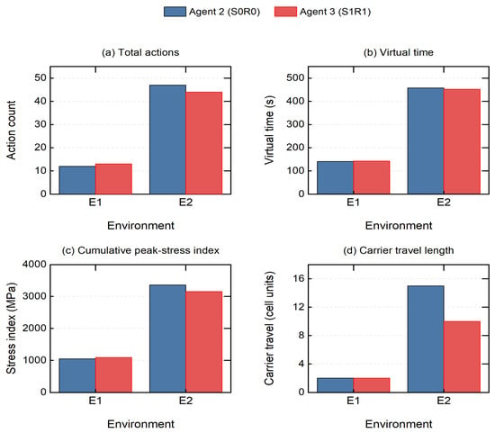
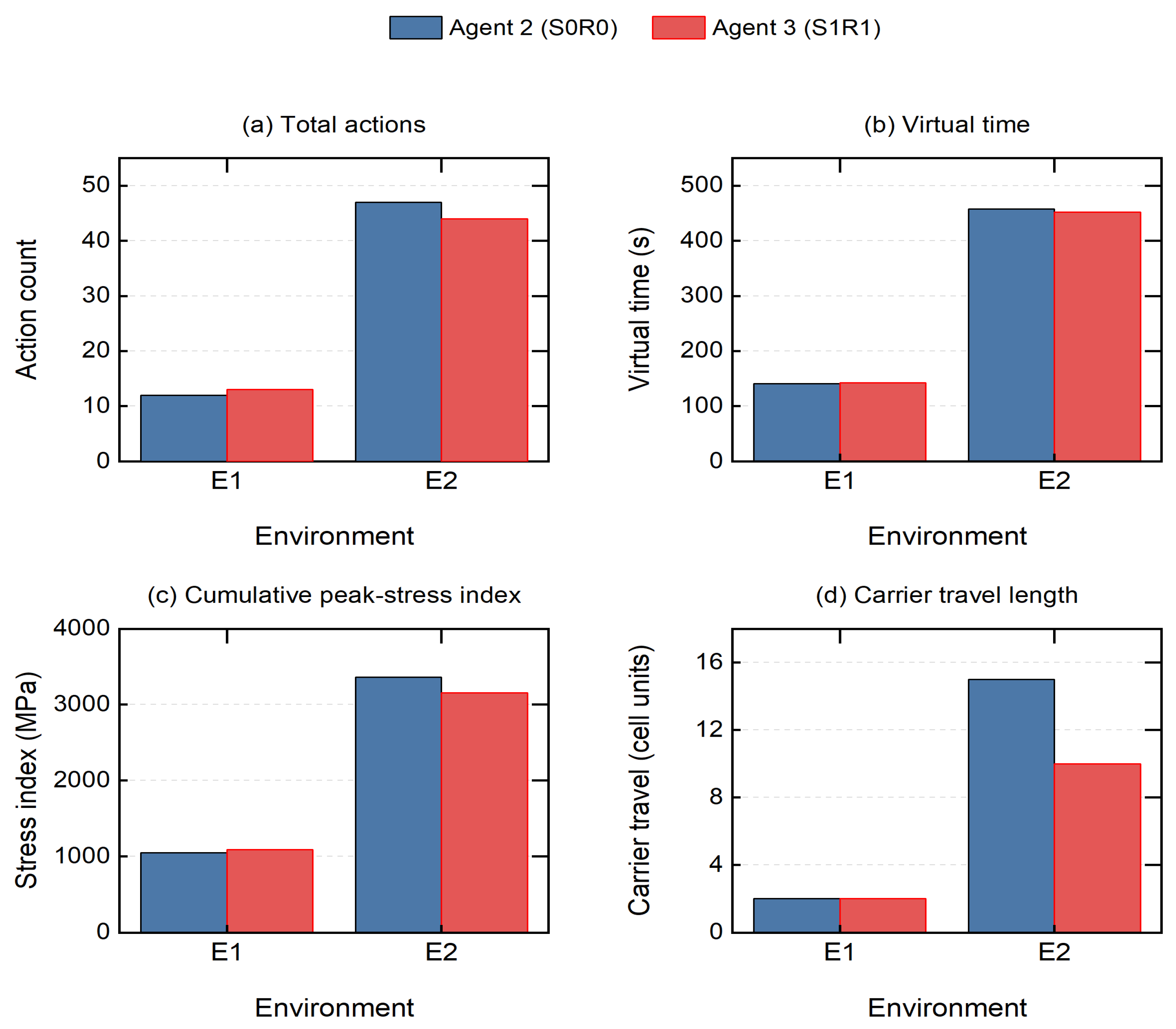
For the archived E2 routes, Agent 3 reduced action count from 47 to 44 (−6.4%), virtual time from 458 to 452 s (−1.3%), and the cumulative peak-stress index from 3361.8 to 3158.0 MPa (−6.1%) relative to Agent 2. Carrier travel was 10 rather than 15 cell units (−33.3%). In E1, Agent 3 required 13 rather than 12 actions, increased virtual time by 1.4%, and increased the index by 4.2%, and carrier travel was 2 cell units for both. Figure 19 compares these four quantities. Carrier travel length counts one-cell translations only, because in-place turns and excavation actions add actions and virtual time but no carrier displacement. It is a grid-unit quantity rather than a field travel distance, and conversion to meters would require a documented physical grid spacing. These are descriptive results for the archived selected routes, distinct from the fixed-budget comparisons in Section 4.4.

Figure 19. Total actions, virtual time, cumulative peak-stress index, and carrier travel length of the archived selected Agent 2 (S0R0) and Agent 3 (S1R1) routes in E1 and E2.

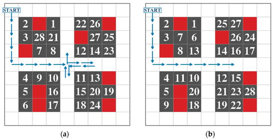
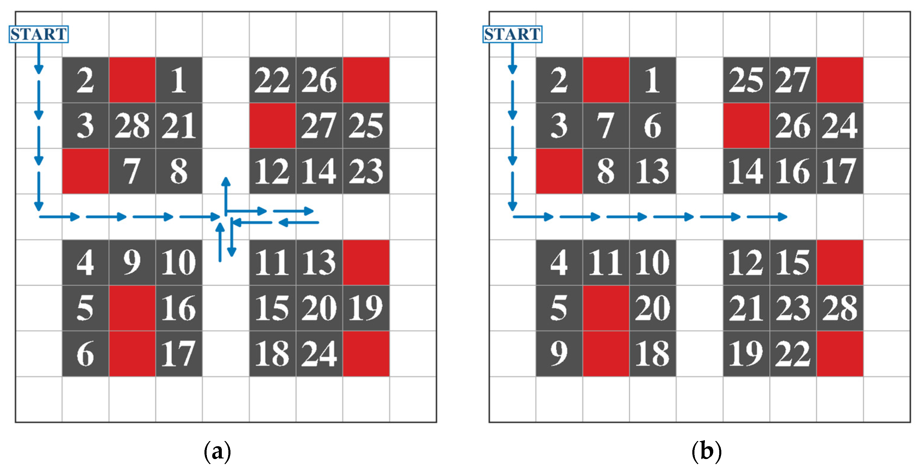
Figure 20 compares the selected E2 routes. Agent 3 used a different sequence of carrier positions and bucket postures and completed the same 28-cell excavation task with three fewer actions than Agent 2.

Figure 20. Selected completed routes in E2: (a) Agent 2 and (b) Agent 3. Blue arrows show carrier travel, dark-gray cells are final non-traversable holes (Figure 14), and white numbers give excavation order. Red cells are obstacles, and START marks the initial carrier cell.

Consistent with the transition rule in Figure 14, every successfully excavated soil cell is shown as a dark-gray, non-traversable hole in the final state. The blue carrier trajectory includes arrowheads to make the direction of travel explicit, while the enlarged in-cell numbers give the chronological order of successful excavation actions. Table 10 and Figure 19 report the corresponding action, virtual-time, and cumulative peak-stress comparisons.

4.3. Site-Derived E3 Environment

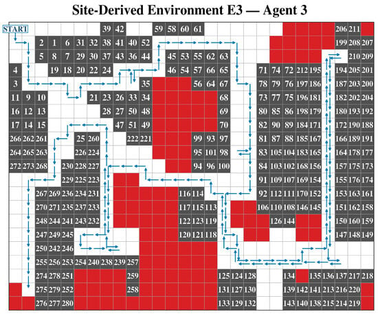
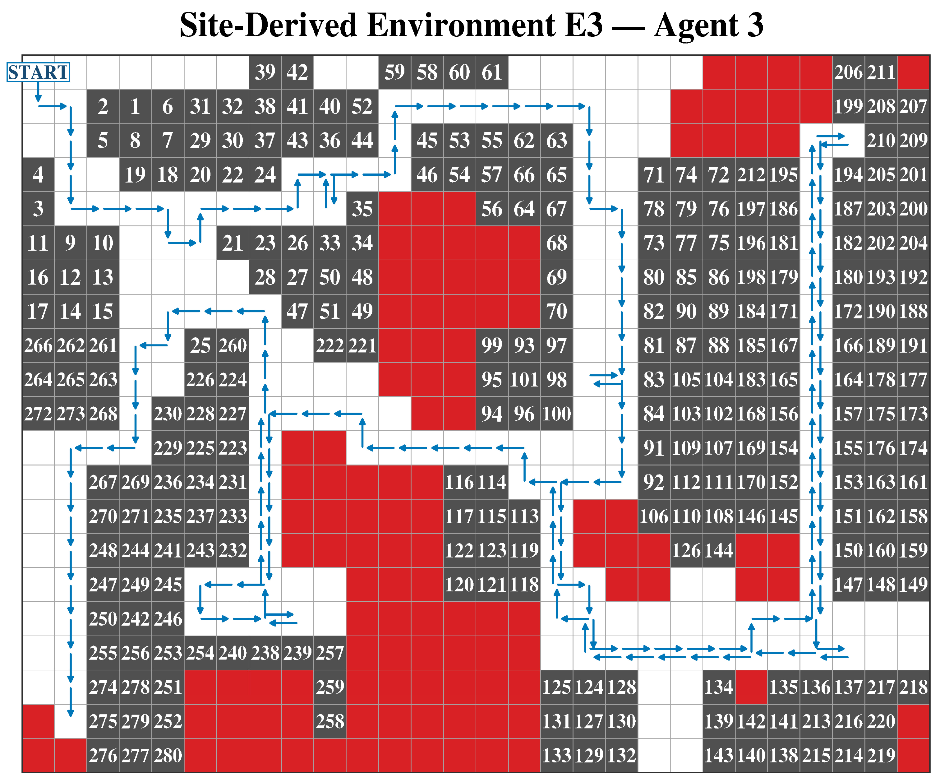
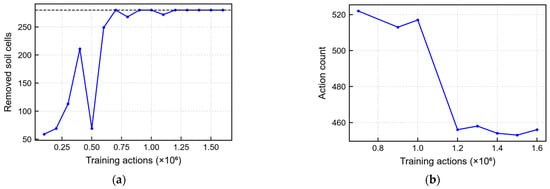
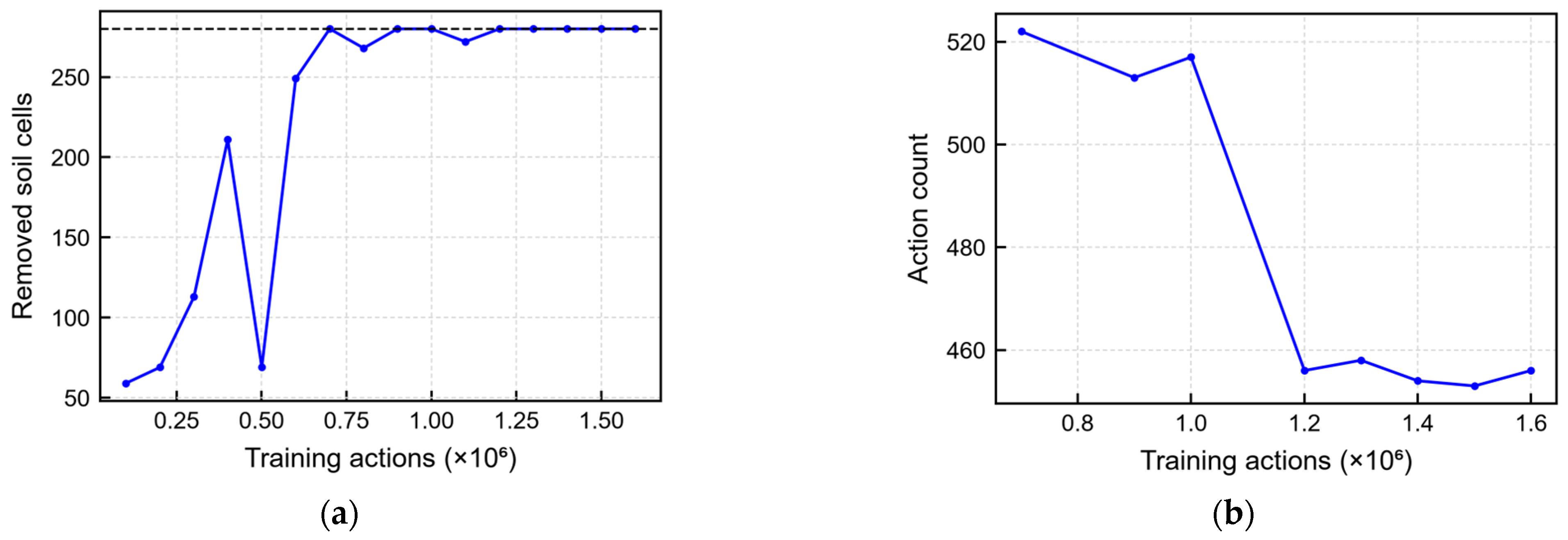
Agent 3 first completed E3 during deterministic evaluation after approximately 0.7 million training actions. After epsilon reached 0.05, the task was completed in each of the five evaluations from 1.2 to 1.6 million training actions, with 453–458 actions per evaluation. The convergence criterion was satisfied at 1,600,084 actions. Figure 21 shows the selected minimum-action completed route. It contained 453 actions: 154 translations, 19 in-place turns, and 280 excavations.

Figure 21. Selected completed Agent 3 route in the 21 × 28 site-derived E3 environment. The blue line denotes carrier motion, and the arrowheads indicate travel direction at intervals along the route. Dark-gray cells are the 280 non-traversable holes produced by successful excavation, consistent with Figure 14. The enlarged white numbers give excavation order, red cells are obstacles, and START identifies the initial carrier cell.

The E3 result confirms that the stress-aware action logic remained computationally feasible when the number of soil cells increased tenfold relative to E2. It does not establish field performance. The geometry was derived from an actual site, but the soil parameters were fixed, the policy was evaluated only in simulation, and only Agent 3 was trained in E3.

The virtual time was 4546 s, the cumulative peak-stress index was 29,604.4 MPa, and no obstacle excavation was recorded. The final-state rendering follows Figure 14: each removed soil cell is a dark-gray non-traversable hole. Arrowheads sampled along the blue trajectory identify the direction of carrier travel, and the enlarged in-cell numbers record excavation order. Figure 22 documents the deterministic evaluation history, and Table 11 reports the learning milestones and complete route-level action breakdown.

Figure 22. Deterministic evaluation history for E3 Agent 3: (a) removed soil cells and (b) action counts of completed evaluations. In panel (a), the black horizontal dashed line marks complete excavation of all 280 soil cells; the light-gray dashed lines in both panels are gridlines.

Figure 22 shows the deterministic evaluation history of E3 Agent 3. The number of removed soil cells reached 280 at the first completed evaluation and remained at this value throughout the final convergence window. The action count of the completed evaluations decreased to 453–458 actions. The principal learning milestones and the selected route are summarized in Table 11.

4.4. Fixed-Budget Ablation and Sensitivity Results

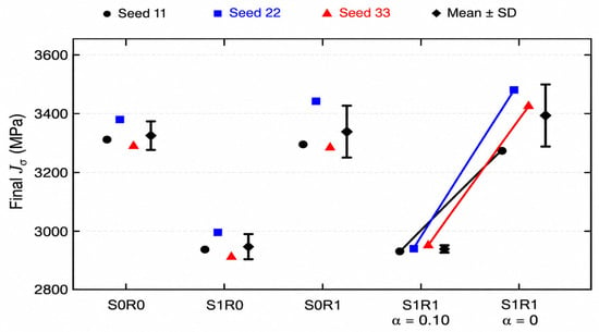
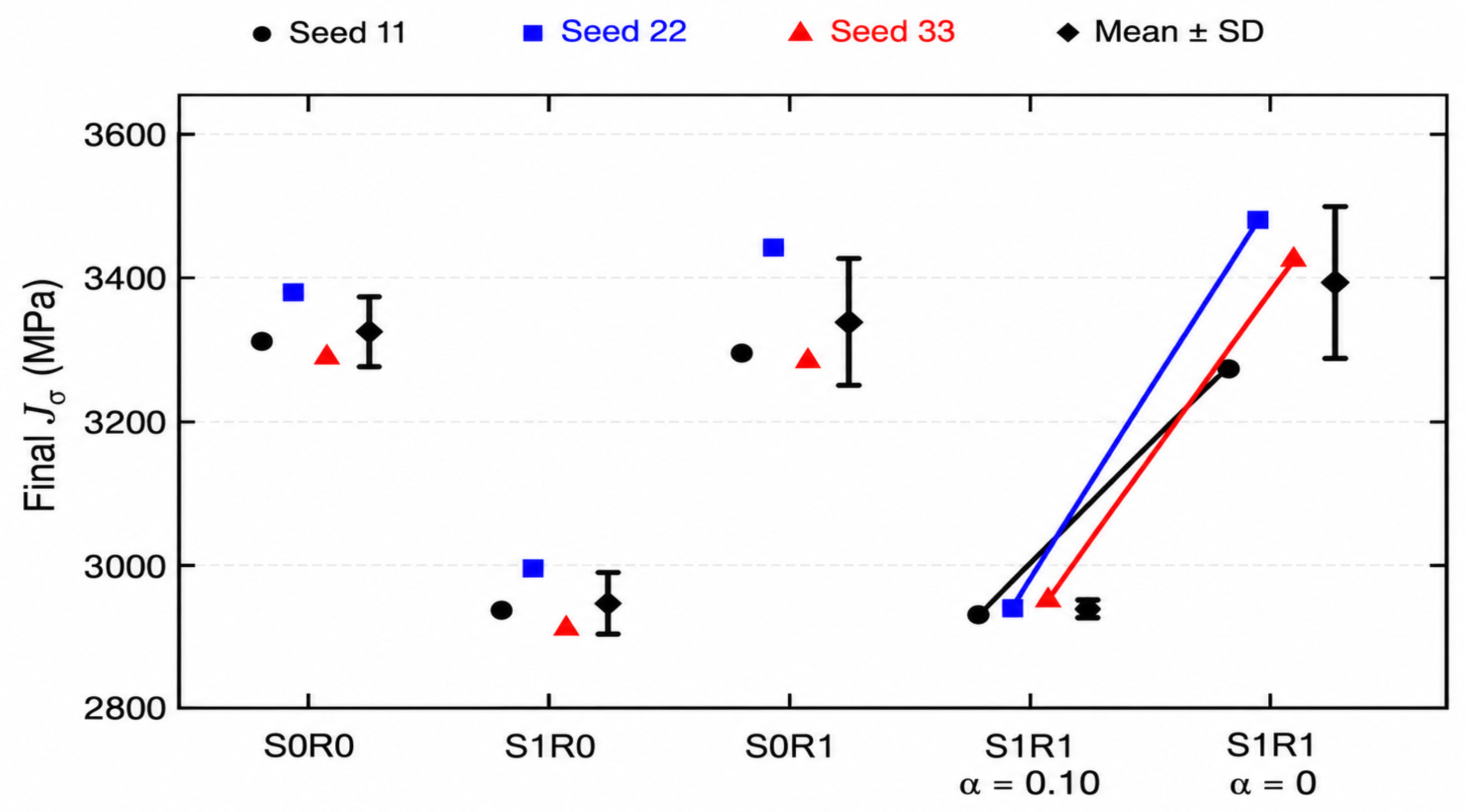
All 21 final policies completed the 28-cell task without obstacle excavation. Table 12 reports the means and sample standard deviations for all seven conditions. The four S/R combinations each required 44 actions and 452 s. S1R1 had a mean index of 2942.30 MPa, compared with 3325.40 MPa for S0R0, a reduction of 383.10 MPa (11.52%) at the same action count and virtual time. The stress package lowered the mean index by 376.90 MPa at R0 and 395.10 MPa at R1, whereas adding the repeat mask changed the index by +12.00 MPa at S0 and −6.20 MPa at S1, with mixed signs across seeds and no final action-count advantage. Removing only the S1R1 penalty gave 3391.93 ± 105.95 MPa, compared with 2942.30 ± 9.61 MPa at α = 0.10, a paired difference of −449.63 ± 99.85 MPa (13.26%); the α = 0 seed-22 policy required 46 actions and 456 s, and all other final policies required 44 actions and 452 s. The reduction is therefore attributable to the stress package and, within it, to the reward penalty, whereas the mask alone provides no consistent benefit.

Table 12. Final-budget E2 analysis set, mean ± sample standard deviation over seeds 11, 22, and 33. All conditions completed 3/3 tasks.

Condition	α	Actions	Virtual Time (s)	Travel (Cells)	Jσ (MPa)
S0R0	—	44.00 ± 0.00	452.00 ± 0.00	10.67 ± 0.58	3325.40 ± 47.99
S1R0	0.10	44.00 ± 0.00	452.00 ± 0.00	11.00 ± 0.00	2948.50 ± 41.12
S0R1	—	44.00 ± 0.00	452.00 ± 0.00	11.00 ± 1.00	3337.40 ± 86.67
S1R1	0.10	44.00 ± 0.00	452.00 ± 0.00	10.33 ± 0.58	2942.30 ± 9.61
S1R1, penalty off	0	44.67 ± 1.15	453.33 ± 2.31	10.67 ± 1.15	3391.93 ± 105.95
S1R1	0.05	44.00 ± 0.00	452.00 ± 0.00	10.67 ± 0.58	3016.17 ± 15.52
S1R1	0.20	44.00 ± 0.00	452.00 ± 0.00	11.00 ± 0.00	2900.27 ± 4.54

Figure 23 shows the individual seed results for the four S/R combinations and the additional penalty-off condition, with lines linking each penalty pair. For S1R1, α = 0.05, 0.10, and 0.20 gave mean indices of 3016.17, 2942.30, and 2900.27 MPa, respectively, with 44 actions and 452 s in all nine runs. The α = 0.20 mean was 42.03 MPa (1.43%) below α = 0.10, so the nominal value obtains about 91% of the reduction reached at α = 0.20 with the smaller weight. The nominal value was retained because it was fixed before the sensitivity study and the smaller weight preserves a larger margin for task completion beyond the tested environment; the results describe the observed trade-off rather than identify an optimum.

Figure 23. Final-policy cumulative peak-stress indices for the four stress/posture-rule combinations and the S1R1 penalty-off condition after 400,000 nominal training actions in E2. Symbols denote seeds 11, 22, and 33, and diamonds and whiskers show the mean ± sample standard deviation (n = 3). Lines connect the same seed at α = 0.10 and α = 0, with the stress inputs and posture rule retained. All 15 policies completed the task, and action and time metrics are reported in Table 12. These values are numerical planning indices.

5. Broader Implications and Limitations

5.1. Mechanical Meaning of the Learned Decision Variable

The stress database converts each MBD result into an attribute of an excavation action. The policy can therefore distinguish two actions that remove the same soil cell but use different attachment postures. The stress range was approximately 50 MPa over the full retained database and approximately 45 MPa within selected relative excavation directions. These differences were large enough to provide a separate structural-response signal to the policy. Because the MBD results were calculated in advance, an MBD simulation was not required at every decision step.

The reported index sums the maximum stress associated with each successful excavation event:

$$J_{\sigma }={\displaystyle \sum _{k=1}^{N_{\mathrm{dig}}}}{\sigma }_{\max ,k}$$

(11)

Here, J_σ denotes the cumulative peak-stress index of the selected route. The term N_dig is the total number of successful excavation events, and σ_max,k is the maximum dynamic stress assigned to the kth successful excavation. The index J_σ can be used to compare routes that share the same task definition. Although it is reported in MPa because it sums event-wise peak stresses, it does not represent a simultaneous structural stress, a rainflow-counted stress history, or a Miner damage sum. A durability assessment would additionally require stress–time histories, material S–N data, mean-stress correction, cycle counting, and experimental strain validation. The present index is therefore interpreted only as relative structural-load exposure.

5.2. Interpretation of Agent Comparisons

E2 provides the clearest internal comparison because it contains obstacles and more alternatives for carrier locations and bucket postures. Agent 3 reduced the action count, virtual time, and J_σ relative to Agent 2. E1 provided fewer route alternatives. In that environment, the posture-repeat constraint could add a turn or require a higher-stress admissible posture. The different E1 and E2 results show that the benefit depends on the available route and posture alternatives.

The 2 × 2 study separates the stress-information package from the repeat constraint, and the α = 0 comparison further isolates the penalty with the inputs and mask retained. The mask did not show a consistent independent index reduction or final action-count benefit. It is therefore retained as a validity constraint that diversifies productive postures, not as a source of efficiency improvement. The zero-penalty comparison supports a contribution from reward shaping under the tested numerical conditions.

Agent 1 is a mechanical baseline rather than a like-for-like learning ablation. Its two-pass requirement for off-axis excavation increased the number of excavation actions in E2 from 28 to 36. Comparisons with Agent 1 therefore quantify the operational consequence of the six-degree-of-freedom attachment model, whereas the Agent 2–Agent 3 comparison addresses the information and policy constraint added to the same 6-DOF capability.

5.3. Advancement Beyond the Previous Korean-Journal Study

The present framework connects a 147-motion database filtered from 225 candidates to excavation decisions that change terrain access. Its action-conditioned Dueling network combines local and navigation information, valid-action advantage averaging, and a conditional posture-repeat rule. Independent nominal loads, CG-based moment transfer, and prescribed retained-soil mass extend the mechanical formulation. E2 and E3 broaden the numerical evaluation, while the seven-condition E2 study examines the planning components and provides a direct penalty comparison. These advances concern engineering integration and numerical assessment. The MBD model and initial stress-informed concept build on [16], and the learning algorithms follow established literature. Denser configuration sampling does not extend the angular range or constitute a new algorithm.

5.4. Limitations and Required Validation

The original E1–E3 route cases used one seed, whereas the additional E2 analysis used three seeds per condition. The small sample limits inference, and more repetitions are needed to assess general superiority or reliable transfer.

E3 was evaluated only with Agent 3 and demonstrates completion at scale rather than superiority over other agents. The soil-load model uses one nominal parameter set and fixed contact geometry; resistance and retained-soil mass follow prescribed ramps. Ground-surface effects, tooth interaction, retained-soil redistribution, and filling momentum exchange are neglected. Frequency correlation does not validate absolute stress magnitude or the physical ranking of configurations. Normalization of stress values does not remove this uncertainty. Hydraulic dynamics, actuator saturation, sensing error, control delay, ground deformation, and machine stability are absent from the numerical planner.

The present study provides an early-stage numerical foundation for incorporating structural-response information into the safety assessment of construction machinery. Experimental validation of the predicted stresses remains an essential next step. We plan to extend the framework to excavators of different capacities, bucket types, and soil conditions, and to investigate its applicability to loaders, dump trucks, and forklifts through equipment-specific models and validation. For experimental validation, we plan to combine strain-gauge measurements with complementary load-identification methods such as transfer path analysis (TPA) for estimating structural stress under representative postures and operating loads. Further studies should also address uncertain soil and timing parameters, appropriate E3 baselines, benchmarks against other learning algorithms such as PPO and SAC, including variants suited to discrete actions, and integration with validated interaction and machine-stability controls. The current results remain conditional on the existing stress database and do not establish absolute stress accuracy, fatigue life, an allowable-stress margin, or field safety.

6. Conclusions

A physics-informed structural-load-aware planning framework was developed for a tilt-rotator-equipped hydraulic excavator. The loading formulation defines independent nominal separation and penetration cases with CG-based force and moment transfer, while gravity acts on a prescribed time-varying dummy mass in the experimentally correlated MBD model. An L₂₅(5²) full-factorial tilt-rotation design was combined with nine relative excavation positions, yielding 225 candidates, of which 147 were retained as admissible motions. Their maximum dynamic stresses ranged from 98.5 to 149.0 MPa, demonstrating that configuration and excavation direction materially alter structural response.

The stress database was embedded in a topology-aware, action-conditioned Dueling DQN. Excavated cells became non-traversable holes, and in-place turning preserved reachability. Local, navigation, multi-step, and randomized-start mechanisms enabled learning in environments ranging from 5 × 5 to 21 × 28 cells. All seven evaluated combinations completed their tasks and met the development convergence criterion.

The original selected-route E2 comparison gave 6.4% fewer actions and a 6.1% lower cumulative peak-stress index for Agent 3, while E1 showed no such improvement. All 21 policies of the additional fixed-budget E2 study, covering seven conditions and three seeds, completed the task. The stress-informed condition (S1R1) and the uninformed baseline (S0R0) both used 44 actions and 452 s, with an 11.52% lower mean index for S1R1. Removing only the penalty raised the mean index by 13.26%, while the repeat rule showed no consistent independent efficiency benefit, and α = 0.20 gave a modest further reduction relative to 0.10. E3 Agent 3 completed 280 excavations in 453 actions with no obstacle excavation.

The study establishes a traceable numerical method for using configuration-dependent structural-response information as a planning variable. The additional comparisons support stress-informed preference shaping within the stated model rather than a universal efficiency advantage. The assumed stress database, three-seed scope, and absence of direct strain validation limit the conclusions. These limits reflect the foundational scope of the present study. Instrumented structural-response validation, combining strain-gauge measurements with complementary methods such as transfer path analysis across excavator capacities and soil conditions, and broader controlled numerical evaluation, including benchmarks against other learning algorithms, remain necessary before claims about field load reduction, durability, or machine safety can be made.

References

- Asghari, V.; Wang, Y.; Biglari, A.J.; Hsu, S.-C.; Tang, P. Reinforcement learning in construction engineering and management: A review. J. Constr. Eng. Manag. 2022, 148, 03122009. [Google Scholar] [CrossRef] [Scilit]
- Hou, P.L.; Lu, F.Y.; Xu, G.N.; Ma, Z.N. Study on spatial mechanics analysis method of excavator attachment with tiltrotator. In Proceedings of the 3rd Annual International Conference on Mechanics and Mechanical Engineering, Chengdu, China, 16–18 December 2016; pp. 215–224. [Google Scholar] [CrossRef] [Scilit][Green Version]
- Huh, J.; Bae, J.; Lee, D.; Kwak, J.; Moon, C.; Im, C.; Ko, Y.; Kang, T.K.; Hong, D. Deep learning-based autonomous excavation: A bucket-trajectory planning algorithm. IEEE Access 2023, 11, 38047–38060. [Google Scholar] [CrossRef] [Scilit]
- Fu, T.; Hu, Z.; Zhang, T.; Bi, Q.; Song, X. Physics-informed neural networks-based online excavation trajectory planning for unmanned excavator. Chin. J. Mech. Eng. 2024, 37, 131. [Google Scholar] [CrossRef] [Scilit]
- Lin, P.; Zhang, L.; Tiong, R.L.K.; Song, X. Physics-guided deep reinforcement learning for improved operation of TBM considering kinetic inertia stability. Adv. Eng. Inform. 2025, 63, 102943. [Google Scholar] [CrossRef] [Scilit]
- Terenzi, L.; Hutter, M. Toward autonomous excavation planning. IEEE Trans. Field Robot. 2024, 1, 292–317. [Google Scholar] [CrossRef] [Scilit]
- Egli, P.; Gaschen, D.; Kerscher, S.; Jud, D.; Hutter, M. Soil-adaptive excavation using reinforcement learning. IEEE Robot. Autom. Lett. 2022, 7, 9778–9785. [Google Scholar] [CrossRef] [Scilit]
- Kurinov, I.; Orzechowski, G.; Hämäläinen, P.; Mikkola, A. Automated excavator based on reinforcement learning and multibody system dynamics. IEEE Access 2020, 8, 213998–214006. [Google Scholar] [CrossRef] [Scilit]
- Choi, G.; Han, S. Reinforcement learning-based dynamic planning of cut and fill operations for earthwork optimization. Autom. Constr. 2023, 156, 105111. [Google Scholar] [CrossRef] [Scilit]
- Liu, Y.; Wang, Y.; Zhou, Z. Simulation of coherent excavator operations in earthmoving tasks based on reinforcement learning. Buildings 2024, 14, 3270. [Google Scholar] [CrossRef] [Scilit]
- Yoon, C.; Ham, Y.; Han, S. Reinforcement learning-driven adaptive 3D simulation and visualization of excavator operations. Autom. Constr. 2026, 181, 106626. [Google Scholar] [CrossRef] [Scilit]
- Ji, M.-G.; Park, J.-K.; Kim, D.-H.; Jung, Y.-H.; Park, J.-K.; Moon, I.-C. Earthwork planning via reinforcement learning with heterogeneous construction equipment. J. Korea Soc. Simul. 2018, 27, 1–13. [Google Scholar] [CrossRef]
- Yao, M.; Feng, X.; Li, P.; Li, Y.; Peng, Z.; Lu, Z. Object-level complete coverage path planning for excavators in earthwork construction. Sci. Rep. 2023, 13, 12818. [Google Scholar] [CrossRef] [Scilit] [PubMed]
- Jelavic, E.; Hutter, M. Whole-body motion planning for walking excavators. In Proceedings of the 2019 IEEE/RSJ International Conference on Intelligent Robots and Systems, Macau, China, 3–8 November 2019; pp. 2292–2299. [Google Scholar] [CrossRef] [Scilit]
- Zhang, W.; Wang, J.; Liu, Y.; Gao, G.; Liang, S.; Ma, H. Reinforcement learning-based intelligent energy management architecture for hybrid construction machinery. Appl. Energy 2020, 275, 115401. [Google Scholar] [CrossRef] [Scilit]
- Kim, D.J.; Oh, J.Y.; Park, H.J.; Chung, J.; Song, C.H. Work path planning of 6-DOF excavator based on multi-body dynamics model. J. Drive Control 2024, 21, 161–173. [Google Scholar] [CrossRef]
- Xing, H.; Xu, Y.; Xie, Y.; Chen, J.; Li, W.; Liu, Y.; Ding, L. Direct Force Compensation-Based Adaptive Hybrid Impedance Control for Dynamic Interaction Environments. IEEE Trans. Autom. Sci. Eng. 2026, 23, 15005–15019. [Google Scholar] [CrossRef] [Scilit]
- Wang, G.; Lin, Z.; Min, F.; Li, D.; Liu, N. Ensuring Safe Physical HRI: Integrated MPC and ADRC for Interaction Control. Actuators 2025, 14, 608. [Google Scholar] [CrossRef] [Scilit]
- Huo, Z.; Yuan, M.; Zhang, S.; Zhang, X. Observer-Based Adaptive Robust Force Control of a Robotic Manipulator Integrated with External Force/Torque Sensor. Actuators 2025, 14, 116. [Google Scholar] [CrossRef] [Scilit]
- Li, Y.; Qi, X. Research on Motion Control of Hydraulic Manipulator Based on Prescribed Performance and Reinforcement Learning. Actuators 2026, 15, 39. [Google Scholar] [CrossRef] [Scilit]
- Wang, T.; Zhu, X.; Shao, F.; He, X.; Zhu, Y. Trajectory Tracking of Autonomous Excavator Based on RBF–PID–Admittance Hybrid Control. Actuators 2026, 15, 424. [Google Scholar] [CrossRef] [Scilit]
- Wang, T.; He, X.; Zhou, Y.; Shao, F. Optimization of Unmanned Excavator Operation Trajectory Based on Improved Particle Swarm Optimization. Actuators 2025, 14, 226. [Google Scholar] [CrossRef] [Scilit]
- Park, B. Development of a Virtual Reality Excavator Simulator: A Mathematical Model of Excavator Digging and a Calculation Methodology. Ph.D. Dissertation, Virginia Polytechnic Institute and State University, Blacksburg, VA, USA, 2002. [Google Scholar]
- Yu, H.S.; Houlsby, G.T. Finite cavity expansion in dilatant soils: Loading analysis. Géotechnique 1991, 41, 173–183. [Google Scholar] [CrossRef] [Scilit]
- Sutton, R.S.; Barto, A.G. Reinforcement Learning: An Introduction, 2nd ed.; MIT Press: Cambridge, MA, USA, 2018. [Google Scholar]
- Bellman, R. A Markovian decision process. J. Math. Mech. 1957, 6, 679–684. [Google Scholar] [CrossRef]
- Watkins, C.J.C.H. Learning from Delayed Rewards. Ph.D. Thesis, University of Cambridge, Cambridge, UK, 1989. [Google Scholar]
- Mnih, V.; Kavukcuoglu, K.; Silver, D.; Rusu, A.A.; Veness, J.; Bellemare, M.G.; Graves, A.; Riedmiller, M.; Fidjeland, A.K.; Ostrovski, G.; et al. Human-level control through deep reinforcement learning. Nature 2015, 518, 529–533. [Google Scholar] [CrossRef] [Scilit] [PubMed]
- Wang, Z.; Schaul, T.; Hessel, M.; van Hasselt, H.; Lanctot, M.; de Freitas, N. Dueling network architectures for deep reinforcement learning. In Proceedings of the 33rd International Conference on Machine Learning, New York, NY, USA, 20–22 June 2016. PMLR 48, 1995–2003. [Google Scholar]
- Kingma, D.P.; Ba, J. Adam: A method for stochastic optimization. In Proceedings of the 3rd International Conference on Learning Representations, San Diego, CA, USA, 7–9 May 2015. [Google Scholar]
Disclaimer/Publisher’s Note: The statements, opinions and data contained in all publications are solely those of the individual author(s) and contributor(s) and not of MDPI and/or the editor(s). MDPI and/or the editor(s) disclaim responsibility for any injury to people or property resulting from any ideas, methods, instructions or products referred to in the content. |
© 2026 by the authors. Licensee MDPI, Basel, Switzerland. This article is an open access article distributed under the terms and conditions of the Creative Commons Attribution (CC BY) license.