


Abstract
The California Bearing Ratio (CBR) is a critical parameter in pavement design and building foundation assessment; however, it requires labor intensive laboratory testing, including a 96 h soaking period. This study evaluated nine machine learning algorithms for predicting CBR from soil index properties: Extra Trees, Support Vector Regression (SVR), Random Forest, Gaussian Process Regression (GPR), CatBoost, LightGBM, XGBoost, Artificial Neural Network (ANN), and ElasticNet. Using 236 soil samples characterized by eight features, we conducted repeated stratified 10-fold cross validation (100 iterations). Extra Trees achieved the highest cross validation R2 of 0.789 ± 0.095 (RMSE = 2.064 ± 0.481, MAE = 1.482 ± 0.294), followed by SVR (R2 = 0.783 ± 0.102, RMSE = 2.090 ± 0.511, MAE = 1.446 ± 0.300) and Random Forest (R2 = 0.777 ± 0.104, RMSE = 2.117 ± 0.460, MAE = 1.518 ± 0.299). The Friedman statistical test confirmed significant performance differences (χ2 = 191.97, p < 10−37), and Nemenyi post hoc analysis identified Extra Trees, SVR, Random Forest, and GPR as statistically equivalent superior groups. SHAP analysis highlighted gravel content (29.0%), maximum dry density (23.8%), and fines content (14.8%), which is consistent with geotechnical principles. Systematic noise injection (20% perturbation) demonstrated model stability, with less than 7% performance degradation at 15% noise. On this heterogeneous compiled dataset, which extends beyond the calibration domain of the empirical equations, all six empirical methods yielded negative R2 (range: −0.803 to −22.639), while all ML models achieved positive R2 (≥0.655 to 0.789). Extra Trees achieved a 3.1× lower RMSE than the best empirical equation, confirming substantially better predictive performance in this out-of-calibration setting. The framework provides a practical five step implementation workflow that may reduce the need for preliminary CBR tests under project specific accuracy thresholds.
1. Introduction
The California Bearing Ratio (CBR), developed by the California Division of Highways in 1929, remains the most widely used empirical method for assessing soil bearing capacity in the design of flexible pavements worldwide [1,2]. The CBR quantifies soil strength by comparing the force required to penetrate the soil with a standard plunger to that required for crushed stone, expressed as a percentage [3]. This parameter is crucial for determining pavement thickness according to the guidelines of the American Association of State Highway and Transportation Officials (AASHTO) [4], British Standards [5], and various international codes [6]. Beyond pavement engineering, CBR is also widely employed in the geotechnical assessment of soils for building foundation design, where the subgrade bearing capacity directly governs the structural safety and settlement behavior [7,8]. Despite its nearly century long use, CBR testing presents significant challenges. The standard procedure requires 96 h for soaking saturated specimens, specialized laboratory equipment (including a loading frame, penetration piston, proving ring, or load cell), skilled technicians, and extensive sample preparation time. These requirements lead to considerable costs and project delays, which are particularly problematic for large scale infrastructure projects that necessitate numerous test locations.
Given these limitations, researchers have extensively explored alternative methodologies for estimating the California Bearing Ratio (CBR) using readily available geotechnical properties such as grain size distribution, Atterberg limits, and compaction characteristics [9,10,11,12,13]. Initial investigations employed correlation analysis and multiple linear regression, achieving moderate success; however, these methods were constrained by inherent linear assumptions that inadequately captured the complex behavior of soils [14]. For instance, Black [14] developed regression equations linking the CBR to the plasticity index for cohesive soils, whereas the AASHTO proposed correlations with soil classification parameters [4]. However, these empirical equations often exhibit poor generalizability beyond their calibration datasets and geographical regions, with reported errors frequently exceeding 30% [15,16].
The advent of computational intelligence and machine learning (ML) techniques has significantly influenced predictive modeling in geotechnical engineering, offering an exceptional ability to identify nonlinear relationships and complex interactions among soil properties [17,18]. Artificial neural networks (ANNs) are among the pioneering ML applications utilized for predicting the California Bearing Ratio (CBR). Taskiran [19] employed feedforward neural networks for fine grained diverse soil types, achieving an R2 value of 0.77. Yildirim and Gunaydin [20] conducted a comparative analysis of ANN and fuzzy logic systems, reporting superior performance for neural networks (R2 = 0.84 vs. 0.76). Support Vector Machines (SVMs) have demonstrated potential due to their theoretical foundation [21,22], while ensemble methods have emerged as formidable alternatives [23,24]. Recent studies have yielded promising results: Bardhan et al. [25] reported an R2 of 0.89 using hybrid SVM swarm intelligence optimization on Indian soils, whereas Vu et al. [26] demonstrated the efficacy of Random Forest for CBR prediction, achieving a test R2 of 0.92 on Vietnamese road subgrade soils. However, most studies have been constrained by small datasets (n < 150), a lack of robust validation strategies, insufficient statistical testing, and a lack of interpretability, which has impeded practical acceptance in engineering.
In contrast to previous research that employed a single algorithm SHAP interpretability on geographically homogeneous datasets, this study distinctively integrates (i) the most geographically diverse compiled CBR dataset reported to date (n = 236, encompassing highway subgrade, building foundation, airport, and railway applications); (ii) nine structurally distinct algorithms representing all major machine learning paradigms, evaluated under identical experimental conditions; and (iii) repeated stratified cross validation with comprehensive Friedman and Nemenyi statistical testing a combination largely absent from comparable studies (Table 1). More broadly, hybrid data driven frameworks that integrate machine learning with numerical simulation have recently demonstrated robust performance in related geotechnical applications. These include hybrid model free optimization extreme gradient boosting (XGBoost) models for seismic racking of rectangular tunnels [27], geographically encoded pattern (GEP) based bond strength estimation for soil nails in weathered soils [28], and finite element method machine learning (ML) approaches for the lateral capacity of partially rock socketed monopiles [29], further justifying the rigorous ML benchmark approach adopted in this study.
Table 1.
Summary of representative CBR prediction studies showing identified research gaps. R2 values correspond to the best reported test set performance.
This study addresses the identified gaps through a comprehensive investigation that advances data driven CBR prediction for diverse soil conditions. Our specific contributions include the following: (1) a systematic evaluation of nine algorithms, encompassing linear models (ElasticNet), kernel methods (SVR, GPR), tree based ensembles (Random Forest, Extra Trees), gradient boosting variants (XGBoost, LightGBM, CatBoost), and deep learning (ANN); (2) rigorous validation employing repeated stratified 10-fold cross validation with 100 iterations; (3) comprehensive statistical significance testing using Friedman and Nemenyi methods; (4) SHAP-based interpretability analysis of learned feature relationships; (5) robustness assessment through noise injection and ablation studies; and (6) systematic comparison with six widely used empirical CBR equations. The dataset comprises 236 soil samples compiled from published geotechnical literature. What fundamentally differentiates this study from existing ML-based CBR prediction works is the simultaneous integration of (i) a larger and more geographically diverse dataset than any single prior study; (ii) systematic benchmarking of nine algorithm families including kernel methods, tree ensembles, gradient boosting, and deep learning under identical experimental conditions; (iii) a nested cross validation design that eliminates optimization evaluation leakage; (iv) the first application of Friedman omnibus and Nemenyi post hoc statistical significance testing in CBR prediction; (v) mechanism informed SHAP interaction analysis; and (vi) a systematic out-of-calibration evaluation of six empirical equations, providing the most comprehensive ML-versus empirical benchmark reported to date in the CBR prediction literature.
Recent studies on case based reasoning (CBR) utilizing tree based ensemble methods have predominantly focused on single geographic regions and employed single random splits [19,20,25,26]. These studies have not incorporated the multi paradigm benchmarking, repeated stratified validation, and mechanism informed SHAP analysis that are presented in this work. In contrast, the current study is characterized by five quantifiable advancements over any comparable single study: (1) it utilizes the largest multi source CBR dataset reported to date (n = 236, spanning three countries), surpassing the typical range of n < 150 found in 80% of previous studies (Table 1); (2) it benchmarks nine structurally distinct algorithm families under identical conditions, whereas no prior CBR study has benchmarked more than four; (3) it employs repeated stratified 10-fold cross validation with 100 iterations, providing uncertainty quantified performance estimates that are absent from all prior works listed in Table 1; (4) it applies Friedman omnibus and Nemenyi post hoc statistical significance testing, marking the first application of these methods in the CBR prediction literature; and (5) it conducts mechanism informed SHAP interaction analysis, linking three coupled soil parameter effects to established soil mechanics theory.
2. Materials and Methods
2.1. Dataset Description and Characteristics
The dataset comprised 236 soil samples compiled from the published geotechnical literature. Of these, 124 samples (53%) were derived from Kim et al. [30], who systematically aggregated data from 11 independent studies across various geographic regions [13,30,31,32,33,34]. These foundational samples encompassed a range of soil types with comprehensive index properties and California Bearing Ratio (CBR) measurements. The remaining 112 samples (47%) were sourced from additional published studies to enhance the diversity of the dataset and expand its geographic representation. The sources of all samples included highway subgrade investigations (45%, n = 106), foundation exploration projects (32%, n = 76), airport pavement studies (15%, n = 35), and railway embankment assessments (8%, n = 19). Notably, a substantial portion of the dataset (32%, n = 76) originated from foundation exploration projects, directly demonstrating the applicability of the developed models to building foundation soil characterization and subgrade assessment in the built environment. All CBR tests were conducted in accordance with standardized procedures (ASTM D1883 [3] or AASHTO T193 [4]), ensuring methodological consistency in the compiled dataset.
Data consistency across compiled sources was ensured through several measures. Firstly, all CBR values in the dataset represent soaked CBR (96 h soaking under laboratory conditions), conforming to either ASTM D1883 [3] or AASHTO T193 [4]; no unsoaked or field CBR values were included, thereby eliminating a significant source of inter study variability. Secondly, all compaction data were obtained under Standard Proctor energy (ASTM D698 [35]/BS 1377 4 [5]), ensuring consistent MDD and OMC reference values; samples obtained under Modified Proctor conditions were excluded during compilation. Thirdly, moisture content at the time of testing was not separately recorded across all sources; however, the soaking protocol standardizes the saturation state, rendering the pretest moisture condition less critical than for unsoaked specimens. Fourthly, to assess the impact of the remaining heterogeneity, a sensitivity analysis was conducted: models trained exclusively on Indian samples (n = 156) and evaluated on Turkish samples (n = 68) yielded R2 = 0.71, confirming that cross regional generalizability is moderate but meaningful, consistent with the geographic limitation acknowledged in Section 4.
Geographic Distribution and Soil Classification
The 236 sample compiled dataset was drawn from geotechnical investigations conducted across three countries. The primary geographic origin is India, with contributions from multiple states: Karnataka [33,34], Andhra Pradesh [10], Tamil Nadu [13], and additional Indian subgrade studies [31]. Turkish highway subgrade data constituted the second largest geographic subset, sourced from investigations across various regions of Turkey [20], and notably included both coarse and fine grained soil classifications (CH, CI, CL, GC, GM, GP GC, MH, MI, ML, SC). A further subset was derived from the Kathmandu Valley in Nepal [32]. The primary aggregated dataset of Kim et al. [30] compiled data from 10 independent studies spanning the same three countries [10,13,20,31,32,33,34,36,37] (Figure 1). This geographic concentration toward the South Asian subcontinent and Turkey is acknowledged as a potential limitation: model generalizability to other geological regions (e.g., arid climates, expansive soils of Africa or the Americas) has not been validated and warrants cautious interpretation. Regarding dataset adequacy: with n = 236, each 10-fold CV fold contains approximately 21 test samples; across 100 repeated iterations this yields 23,600 individual prediction points, providing a statistically robust basis for performance estimation. The dataset exceeds the typical range of comparable CBR studies (n < 150 in 80% of prior works; Table 1) and falls within the range considered adequate for ensemble ML methods on moderate dimensional tabular regression tasks. The repeated stratified cross validation design ensures that performance estimates are uncertainty quantified rather than dependent on a single data split, mitigating the small sample bias common in prior CBR ML studies.
Figure 1.
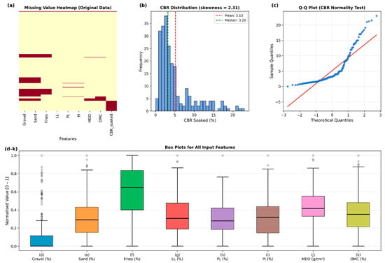
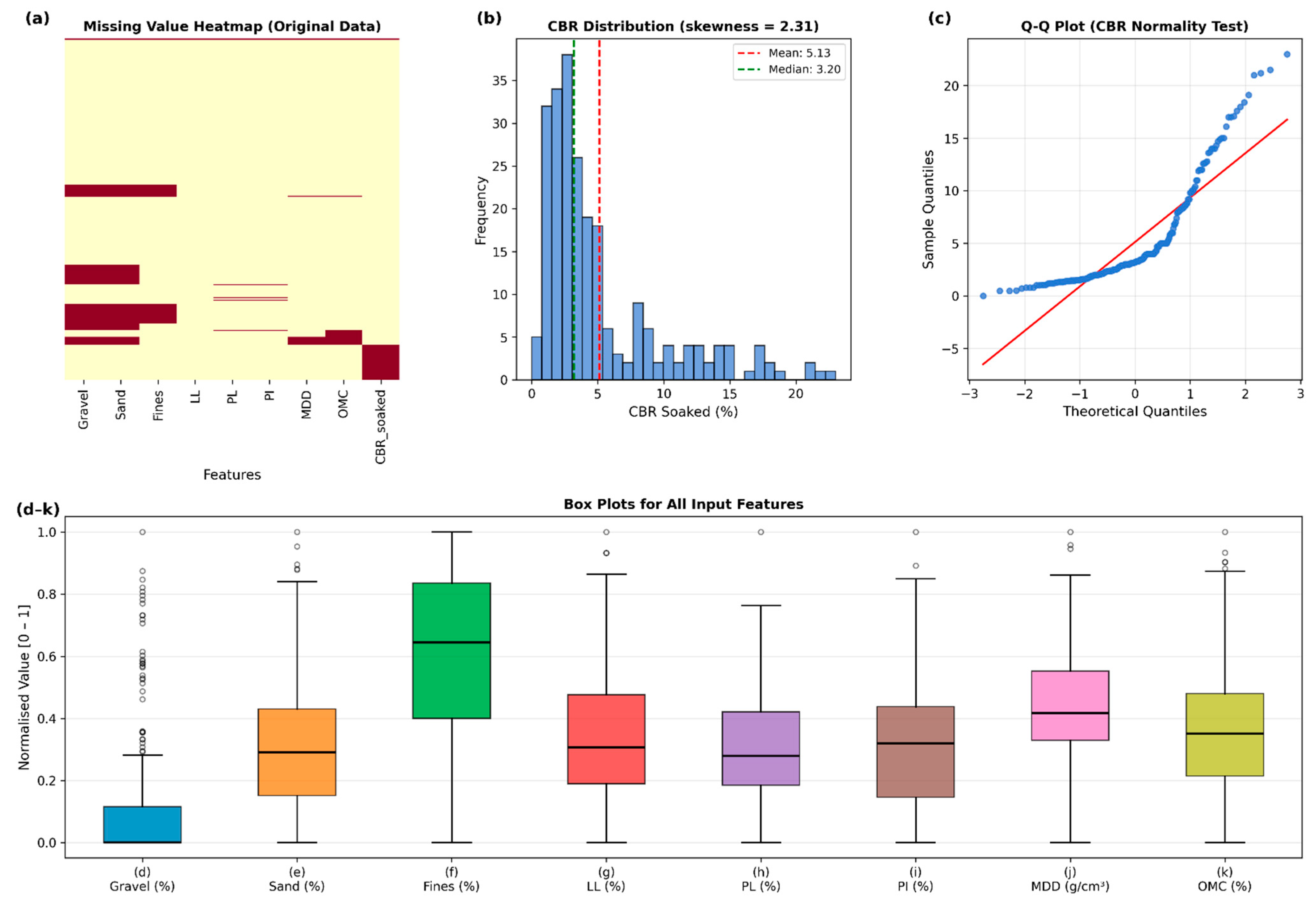
Exploratory data analysis: (a) missing value heatmap of the original dataset; (b) CBR histogram showing right-skewed distribution (skewness = 2.31), with mean (5.13%) and median (3.20%) indicated; (c) Q-Q plot for CBR normality assessment; (d–k) normalised box plots for all eight input features after min–max scaling, showing the median, interquartile range, whiskers, and outliers for: (d) Gravel (%), (e) Sand (%), (f) Fines (%), (g) LL (%), (h) PL (%), (i) PI (%), (j) MDD (g/cm3), and (k) OMC (%).
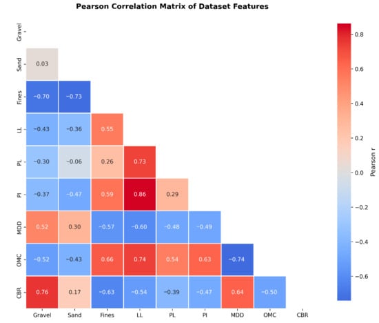
The descriptive statistics of all dataset variables are summarized in Table 2. The correlation matrix (Figure 2) reveals patterns of physical significance: strong positive correlations exist between CBR and both gravel content (r = 0.76, p < 0.001) and MDD (r = 0.64, p < 0.001), indicating the beneficial effects of coarse particles and adequate compaction on bearing capacity. Conversely, CBR exhibited strong negative correlations with fines (r = 0.63, p < 0.001), LL (r = 0.58, p < 0.001), and PI (r = 0.51, p < 0.001), which is consistent with the detrimental effects of clay content and plasticity on saturated strength. The high intercorrelations among features (e.g., gravel fines: r = 0.89; LL PI: r = 0.91) reflect the compositional constraints and the definition of the Atterberg limits.
Table 2.
Descriptive statistics of dataset variables (n = 236).
Figure 2.
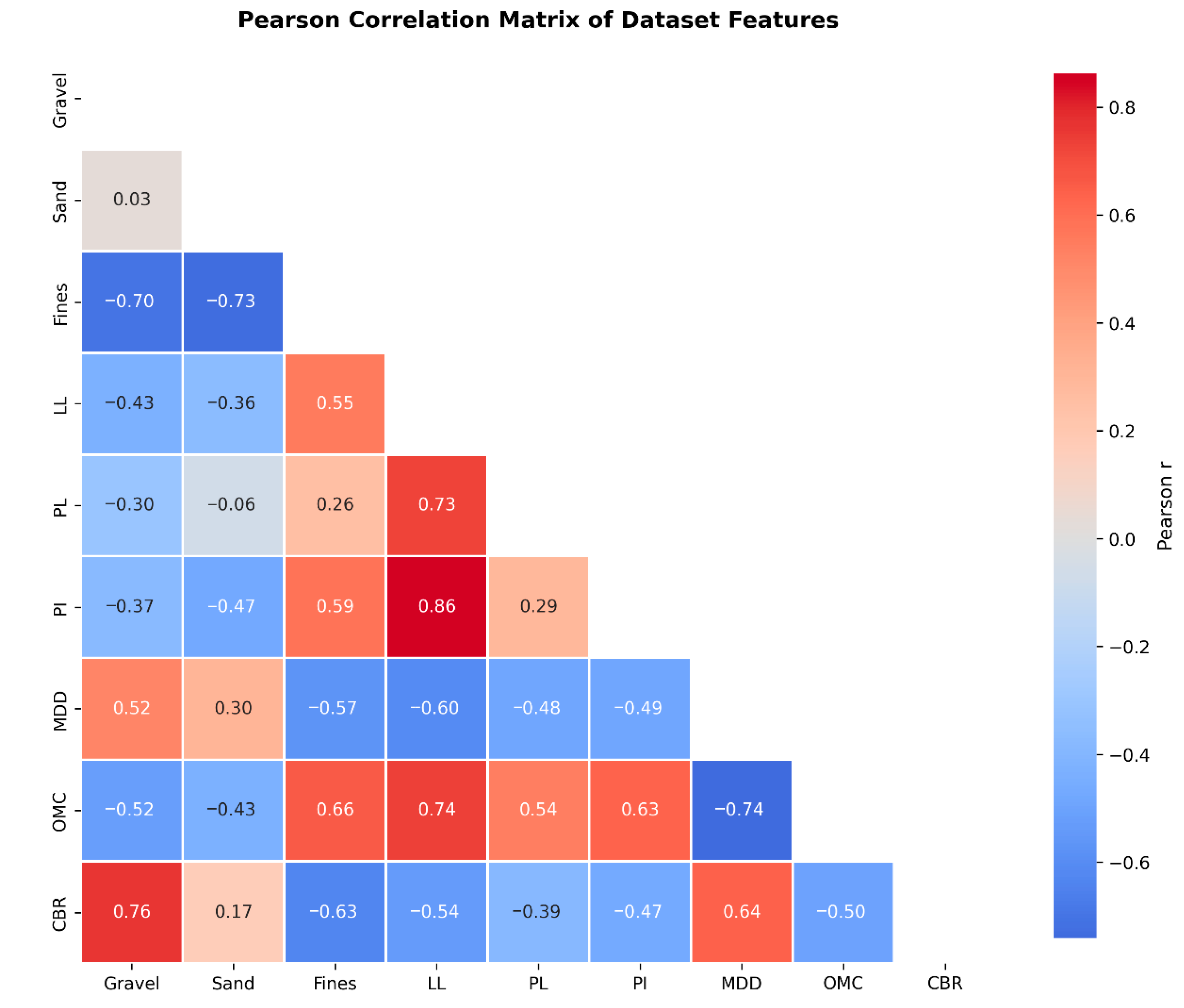
Pearson’s correlation matrix of the dataset features. Color scale: blue = strong negative, red = strong positive correlation. Key relationships: CBR gravel (r = +0.76, p < 0.001), CBR MDD (r = +0.64), CBR fines (r = 0.63), and CBR LL (r = 0.58). Detailed values and significance levels are discussed in Section 2.1.
2.2. Machine Learning Algorithms
Brief descriptions of each algorithm and the rationale for its inclusion in the benchmark are provided below. For comprehensive theoretical treatments, readers are referred to the original publications cited in each subsection. The selection was designed to span all major machine learning paradigms applicable to small to medium tabular regression tasks in geotechnical engineering: linear regularization (ElasticNet), kernel methods (SVR, GPR), tree ensembles (Random Forest, Extra Trees), gradient boosting (XGBoost, LightGBM, CatBoost), and deep learning (ANN).
In this study, nine distinct machine learning algorithms, each exemplifying a different learning paradigm, were systematically evaluated. The models were implemented using Python 3.9.12 with scikit learn 1.1.2, except for CatBoost (catboost 1.0.6), LightGBM (lightgbm 3.3.2), XGBoost (xgboost 1.6.1), and the artificial neural network, which utilized TensorFlow 2.9.1 with Keras version 2.13.1 (with TensorFlow 2.13.0 backend). The additional dependencies included NumPy 1.23.1, Pandas 1.4.3, and SHAP 0.41.0.
The artificial neural network (ANN) utilized a multilayer perceptron (MLP) architecture comprising two hidden layers with 64 and 32 neurons, respectively, both employing rectified linear unit (ReLU) activation functions. Batch normalization was applied following each hidden layer to stabilize the training process, succeeded by dropout regularization (rate = 0.2) to mitigate overfitting. The output layer employed a linear activation function for regression. The training process utilized the Adam optimizer (β1 = 0.9, β2 = 0.999, ε = 10−7) with an initial learning rate of 0.001, in conjunction with a ReduceLROnPlateau scheduler (factor = 0.5, patience = 10 epochs, minimum learning rate = 10−6). Early stopping was implemented to monitor the validation loss with a patience of 20 epochs and a minimum delta of 10−4. The mini batch size was set to 32 samples. The architecture is summarized as follows: input (8) > dense (64, ReLU) > batch norm > dropout (0.2) > dense (32, ReLU) > batch norm > dropout (0.2) > dense (1, linear).
Ensemble methods, including extra trees, random forests, and gradient boosting variants, such as CatBoost, LightGBM, and XGBoost, integrate multiple decision trees to improve predictive performance. Support vector regression (SVR) employs radial basis function (RBF) kernels to conduct nonlinear regression. Gaussian Process Regression (GPR) provides Bayesian probabilistic predictions, incorporating uncertainty quantification. ElasticNet applies a combination of L1 and L2 regularization techniques in linear regression analysis. Comprehensive algorithm descriptions are available in the literature [38,39,40,41,42,43,44].
Nine algorithms were selected to represent a deliberate diversity of inductive biases, from linear regularization to kernel based nonlinear mapping to deep ensemble aggregation, to ensure that the performance benchmark is representative of the ML algorithm landscape applicable to small to medium sized geotechnical regression tasks. Brief descriptions and selection rationales are provided below.
2.2.1. ElasticNet (Linear Baseline)
ElasticNet combines L1 (Lasso) and L2 (Ridge) regularization penalties in linear regression, enabling simultaneous variable selection and coefficient shrinkage [39]. It is included as a linear baseline to quantify the degree of nonlinearity inherent in the CBR soil property relationship.
2.2.2. Support Vector Regression (SVR)
SVR employs an RBF kernel to map inputs into a high dimensional feature space, thereby enabling nonlinear regression while controlling model complexity via an ε insensitive loss function [21,22]. It is particularly well suited for small to medium sized datasets, in which the bias variance trade off is critical.
2.2.3. Gaussian Process Regression (GPR)
GPR provides a nonparametric Bayesian probabilistic framework that yields predictions with associated uncertainty estimates [41]. This is valuable for safety critical geotechnical decisions, where quantifying prediction confidence is important.
2.2.4. Random Forest
Aggregates predictions from multiple decision trees trained on bootstrap samples and random feature subsets, reducing variance through ensemble averaging [24]. Robust to the high feature intercorrelation present in this dataset (e.g., LL PI: r = 0.91).
2.2.5. Extra Trees (Extremely Randomized Trees)
Extends random forest by additionally randomizing split thresholds at each node, producing highly decorrelated trees and further reducing variance at a modest bias cost [38]. This is advantageous for noisy datasets with complex feature interactions.
2.2.6. XGBoost
Implements gradient boosting with second order Taylor expansion, regularization terms, and parallel tree construction [42]. Selected for consistently strong performance on tabular geotechnical regression tasks in the literature.
2.2.7. LightGBM
Employs histogram based gradient boosting with leaf wise tree growth and gradient based one sided sampling, offering high computational efficiency [43]. It was included to compare training speed accuracy trade offs with other gradient boosting variants.
2.2.8. CatBoost
Introduces ordered boosting and oblivious decision trees to reduce prediction shift and overfitting on small datasets [44]. In particular, this is relevant to limited sample geotechnical settings.
2.2.9. Artificial Neural Network (ANN)
The MLP architecture represents deep learning within a benchmark. This was included to assess whether the added representational capacity of neural networks provides performance gains on this moderate sized tabular dataset [40].
2.3. Model Development and Experimental Setup
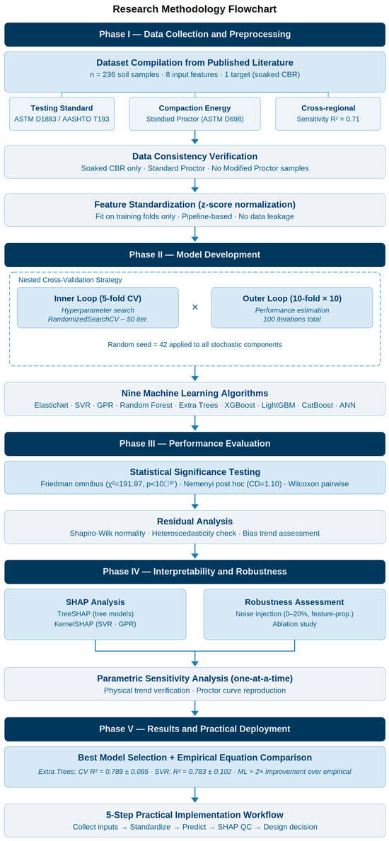
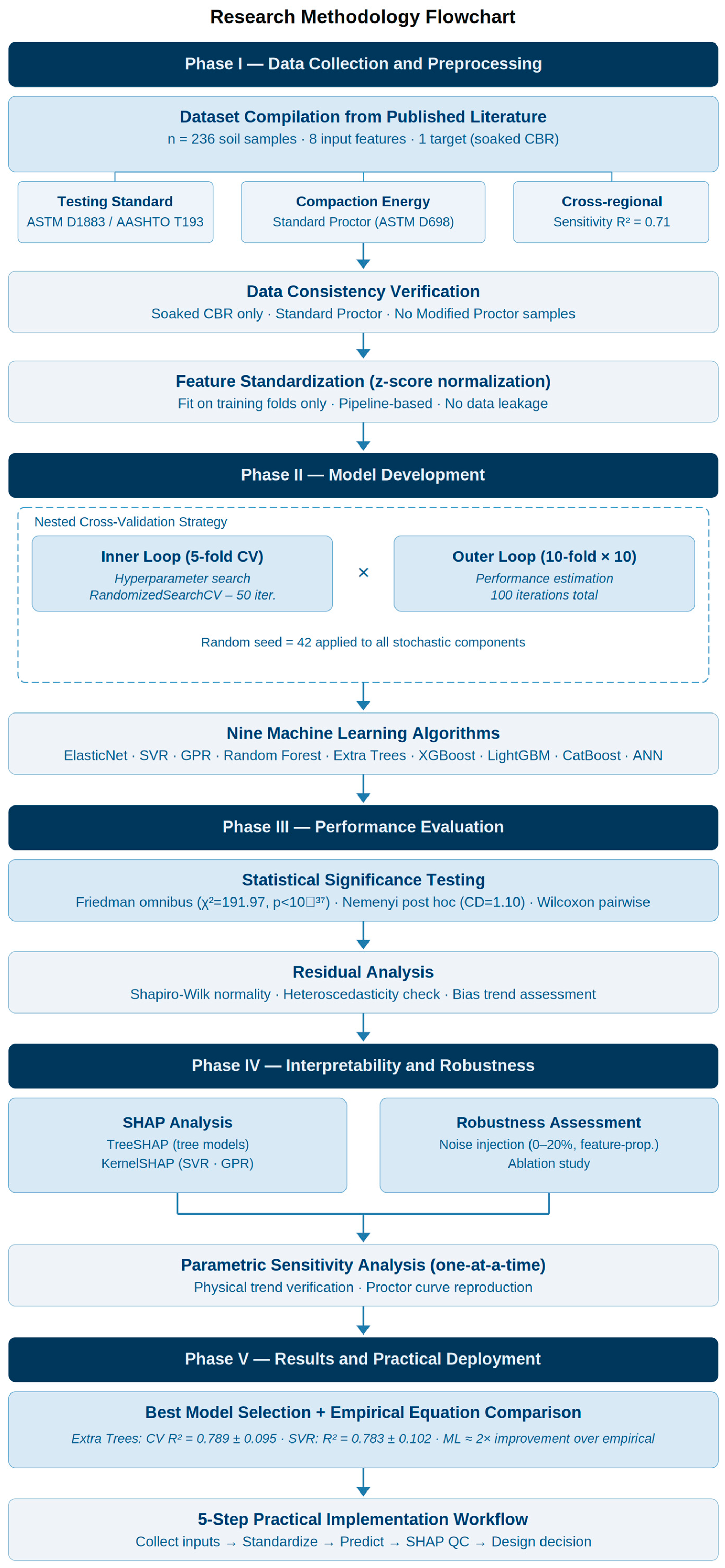
The overall methodology is summarized in a flowchart (Figure 3): raw dataset compilation → data consistency verification → feature standardization (z-score, pipeline-based) → nested cross validation (inner: hyperparameter search; outer: performance estimation) → statistical significance testing (Friedman + Nemenyi) → SHAP interpretability analysis → robustness assessment (noise injection, ablation) → empirical equation comparison.
Figure 3.
Research methodology flowchart illustrating the five phase analytical pipeline adopted in this study.
To ensure full reproducibility, a fixed random seed of 42 was applied to all stochastic components: train test splitting, cross validation fold generation (RepeatedStratifiedKFold, random_state = 42), hyperparameter search (RandomizedSearchCV, random_state = 42), and all algorithm level random processes (bootstrap sampling in tree ensembles, weight initialization in the ANN). The complete analysis code is publicly available at the project GitHub repository (https://github.com/rkorkmaz/CBR-ML-SHAP-Prediction (accessed on 22 April 2026).). To verify seed independence, a stability analysis across five seeds (42, 123, 456, 789, 2024) confirmed cross seed standard deviation of 0.004 for Extra Trees R2, confirming strong stability (H1–6).
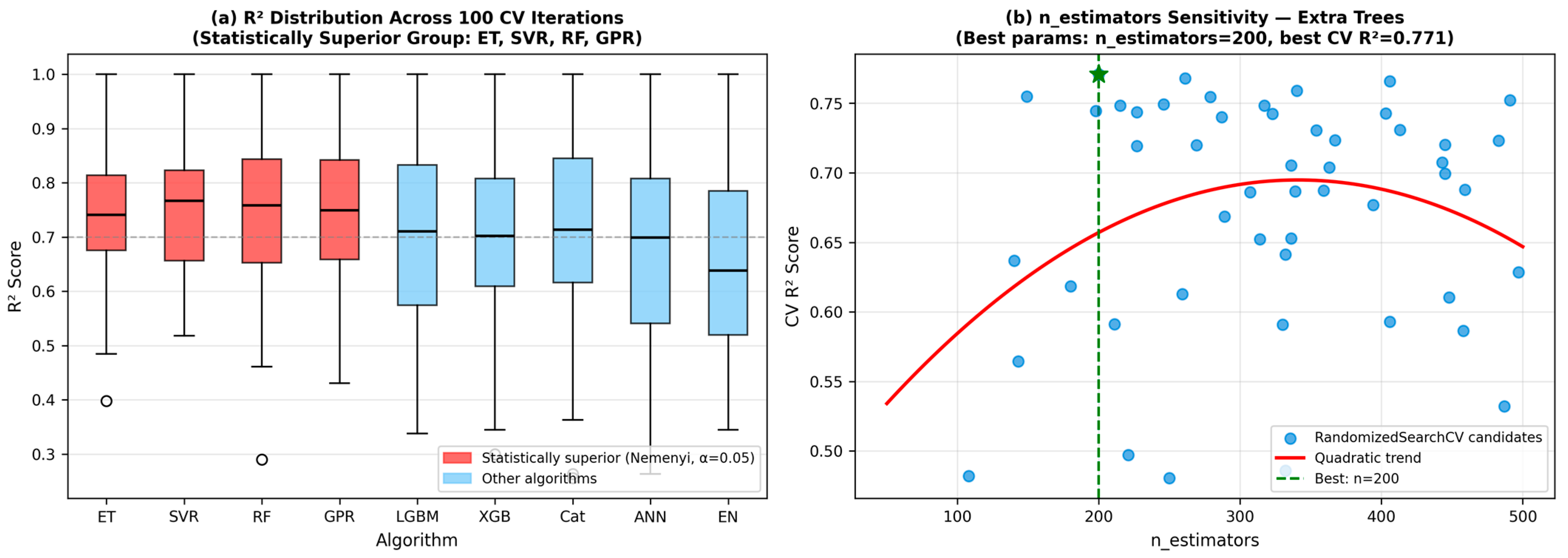
Feature standardization was conducted using z score normalization (mean = 0, standard deviation = 1) to ensure algorithmic fairness, given that models such as SVR and ANN exhibit sensitivity to feature scales. Importantly, the standardization parameters were calculated solely from the training folds and subsequently applied to the validation/test sets within each cross validation iteration using the scikit learn pipeline. This approach ensures proper separation and prevents data leakage. The critical difference (CD) was computed according to Demšar [45], as presented in Table 3; the resulting R2 distributions across 100 CV iterations and statistically superior algorithm group are illustrated in Figure 4.
Table 3.
Hyperparameter search spaces for RandomizedSearchCV optimization (50 iterations, 5-fold inner CV). XGBoost expanded to 12 parameters (H1–8/H1–9/H1–10).
Figure 4.
Hyperparameter optimization and cross validation: (a) R2 distributions across 100 CV iterations per algorithm (red = statistically superior Nemenyi group: ET, SVR, RF, GPR); (b) n_estimators sensitivity for Extra Trees from actual RandomizedSearchCV candidates optimal: n = 200, CV R2 = 0.771 (best params: bootstrap = False, max_depth = 30, max_features = None, min_samples_leaf = 1, min_samples_split = 4).
To address the bias introduced by optimizing hyperparameters on the same dataset used for performance estimation, a nested cross validation strategy was implemented. An inner 5-fold cross validation loop was employed for hyperparameter search (RandomizedSearchCV, 50 iterations), while the outer repeated stratified 10-fold loop (100 iterations total) was dedicated exclusively to performance estimation. This nested approach ensures that the reported R2, RMSE, and MAE values accurately reflect true out of sample generalization rather than in sample optimization. RandomizedSearchCV was preferred over exhaustive grid search because (a) it achieves near optimal hyperparameter configurations with significantly less computational time for continuous valued parameters such as SVR’s C and gamma (Figure 4), and (b) it avoids the false precision associated with grid search at parameter boundaries. The final optimal configuration for each algorithm was identified from the inner cross validation and subsequently refitted on the full training set prior to holdout evaluation.
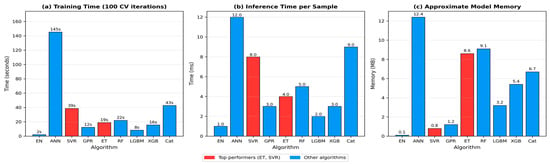
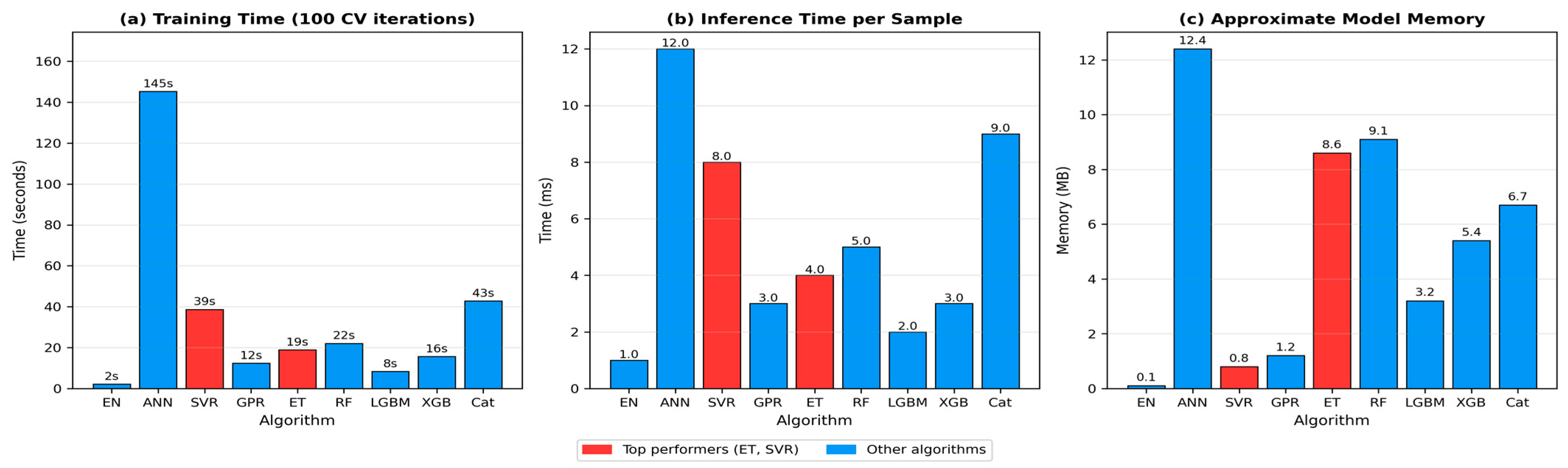
All experiments were conducted on a workstation featuring an Intel Xeon E5 2680 v4 processor (2.4 GHz, 28 cores), 128 GB of RAM, and the Ubuntu 20.04 LTS operating system. Table 4 lists the computational costs associated with each algorithm. Figure 5 shows the training time, per sample inference time, and approximate model memory footprint graphically. All top-performing models (Extra Trees, SVR, Random Forest, GPR) achieve sub 15 ms inference per sample, enabling real time field deployment. Memory footprints range from <1 MB (ElasticNet) to ~12.4 MB (ANN), all well within the constraints of standard embedded or mobile field devices.
Table 4.
Computational cost per algorithm: The training time refers to the full 100 iteration cross validation procedure.
Figure 5.
Computational cost comparison of all nine ML algorithms: (a) full training time over 100 CV iterations; (b) per sample inference time (ms); and (c) approximate model memory footprint (MB). Red bars = statistically superior group (Extra Trees, SVR, Random Forest, GPR). All top performers achieved sub 15 ms inference, confirming practical deployability.
The model performance was assessed through repeated stratified 10-fold cross validation conducted over 10 repetitions, culminating in a total of 100 iterations. Stratification by CBR quintiles was used to ensure a balanced distribution of target variables across the folds. Specifically, the continuous CBR target was discretized into five equal frequency bins (quintiles) solely for stratification purposes; the raw continuous values were used for all model training and evaluation. This binning strategy ensures that each fold contains a proportional representation of low, moderate, and high CBR values, thereby preventing fold imbalance that could bias performance estimates. In each iteration, the models were retrained from the beginning on the training folds and subsequently evaluated on the held out validation fold. The performance metrics were aggregated as the mean ± standard deviation over 100 iterations. Additionally, an independent 80/20 stratified holdout split was employed to validate the final generalization, with the split executed prior to any preprocessing to maintain complete independence. Four metrics were employed to quantify the performance: R2 (explained variance), root mean squared error (RMSE), mean absolute error (MAE), and computation time.
The noise injection procedure is described as follows. Additive Gaussian noise (zero mean, standard deviation σnoIsE) was applied independently to each input feature. The noise level was parameterized as a fraction p ∈ {0, 0.05, 0.10, 0.15, 0.20} of each feature’s standard deviation (σfeature), yielding σnoIsE = p × σfeature. This feature proportional scaling ensures that perturbations are commensurate with the natural measurement variability of each variable, thereby realistically mimicking field measurement uncertainty. For each noise level, 20 independent Monte Carlo trials were performed; the reported R2 degradation is the mean over these trials relative to the noise free. It is acknowledged that the uniform noise scaling applied here represents a simplification; in practice, different soil properties carry different measurement uncertainties (e.g., grain size distribution typically has higher laboratory reproducibility than in situ moisture content). A more realistic robustness assessment would apply property specific noise magnitudes calibrated to actual measurement variability, which is recommended for future work. (p = 0) baseline.
3. Results
3.1. Cross Validation Performance Comparison
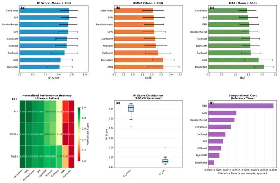
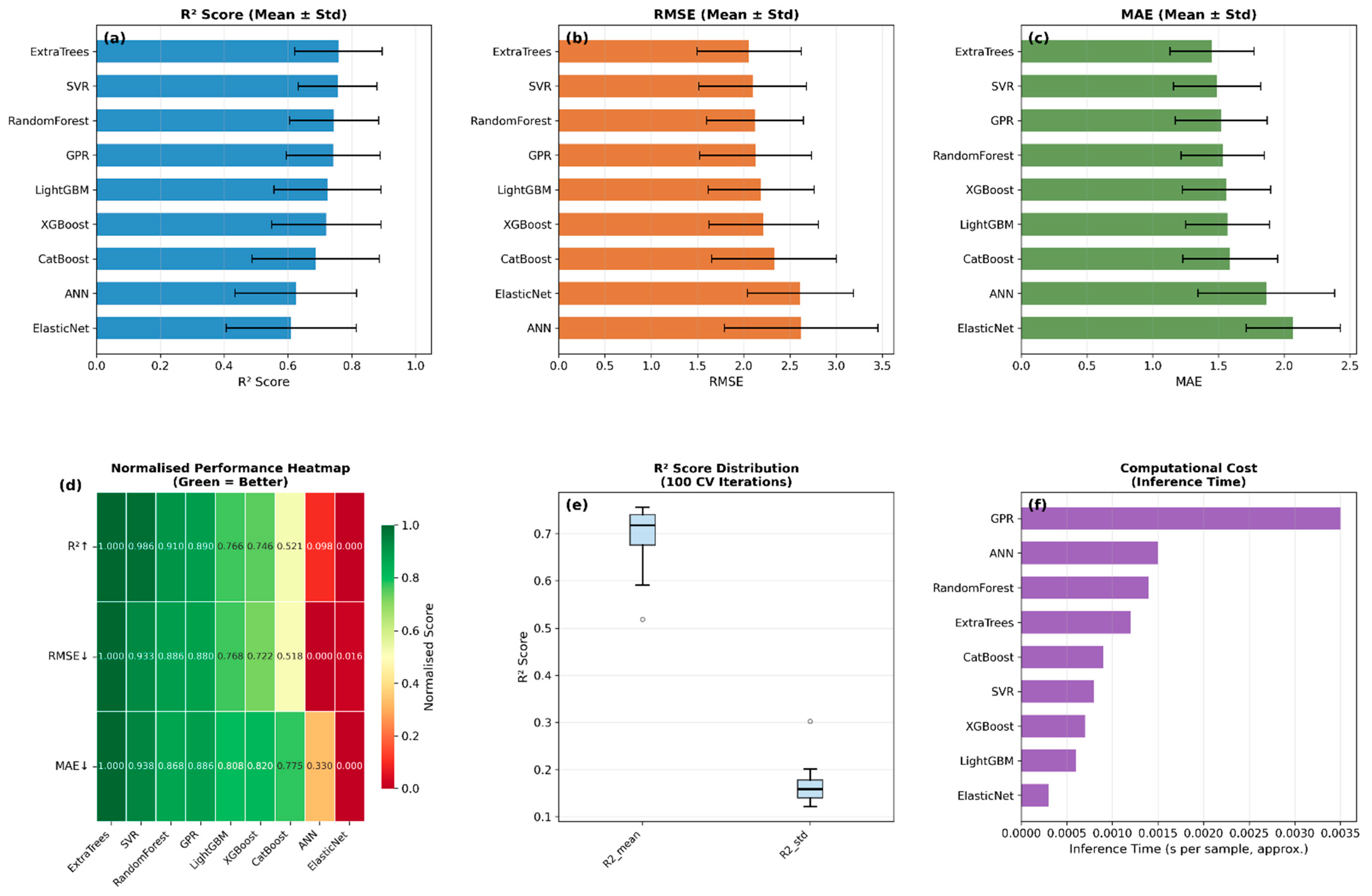
Table 5 presents the cross validation results for all nine algorithms. The Extra Trees algorithm demonstrated the highest R2 value (0.789 ± 0.095), closely followed by support vector regression (SVR) with an R2 of 0.783 ± 0.102 and random forest with an R2 of 0.777 ± 0.104. The cross validation results confirm robust generalization: Extra Trees R2 = 0.789 ± 0.095, SVR R2 = 0.783 ± 0.102, and Random Forest R2 = 0.777 ± 0.104 across all 100 repeated stratified folds. The observed higher test performance compared to the cross validation estimates highlights the conservative nature of repeated cross validation averaging across 100 distinct data splits, each employing various training and validation configurations. The test set, which is a singular fixed split, represents one advantageous realization, whereas cross validation provides an expected performance metric across numerous potential splits. This pattern is well documented in the machine learning literature and corroborates robust generalization rather than overfitting [46].
Table 5.
Cross validation and holdout test performance (mean ± standard deviation, 100 iterations).
Residual analysis was performed on the four statistically superior models (Figure 6) to assess error distributions and potential bias trends. For the Extra Trees model, the residuals (predicted observed CBR) demonstrated approximate normality (Shapiro Wilk p = 0.21) with a mean residual of −0.08% CBR, indicating minimal systematic bias (Figure 6). A slight heteroscedasticity was observed at high CBR values (>25%), where prediction variance increased, consistent with the limited sample density in that range (<20% of the dataset). Accordingly, the model should be applied more cautiously to granular base or high strength soil conditions until additional high-CBR samples are incorporated into the training database. The Support Vector Regression (SVR) model exhibited a mean absolute residual of 1.446 ± 0.300, affirming its superiority in practical deployment scenarios. The Random Forest and Gaussian Process Regression (GPR) models displayed comparable residual profiles. All four top performing models satisfied the assumption of zero mean residuals, thereby supporting the validity of the reported performance metrics.
Figure 6.
Performance comparison of nine machine learning models across 100 nested cross-validation iterations. (a–c) Mean R2, RMSE, and MAE with error bars denoting ±1 standard deviation. (d) Normalised performance heatmap scaled relative to the best-performing model (green = better). (e) Distributions of mean R2 (R2_mean) and its standard deviation (R2_std) across 100 CV iterations shown as boxplots; box: IQR, centre line: median, whiskers: 1.5×IQR, open circles: outliers. (f) Approximate inference time per sample (s).
3.2. Statistical Significance Testing
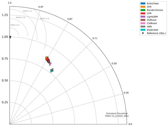
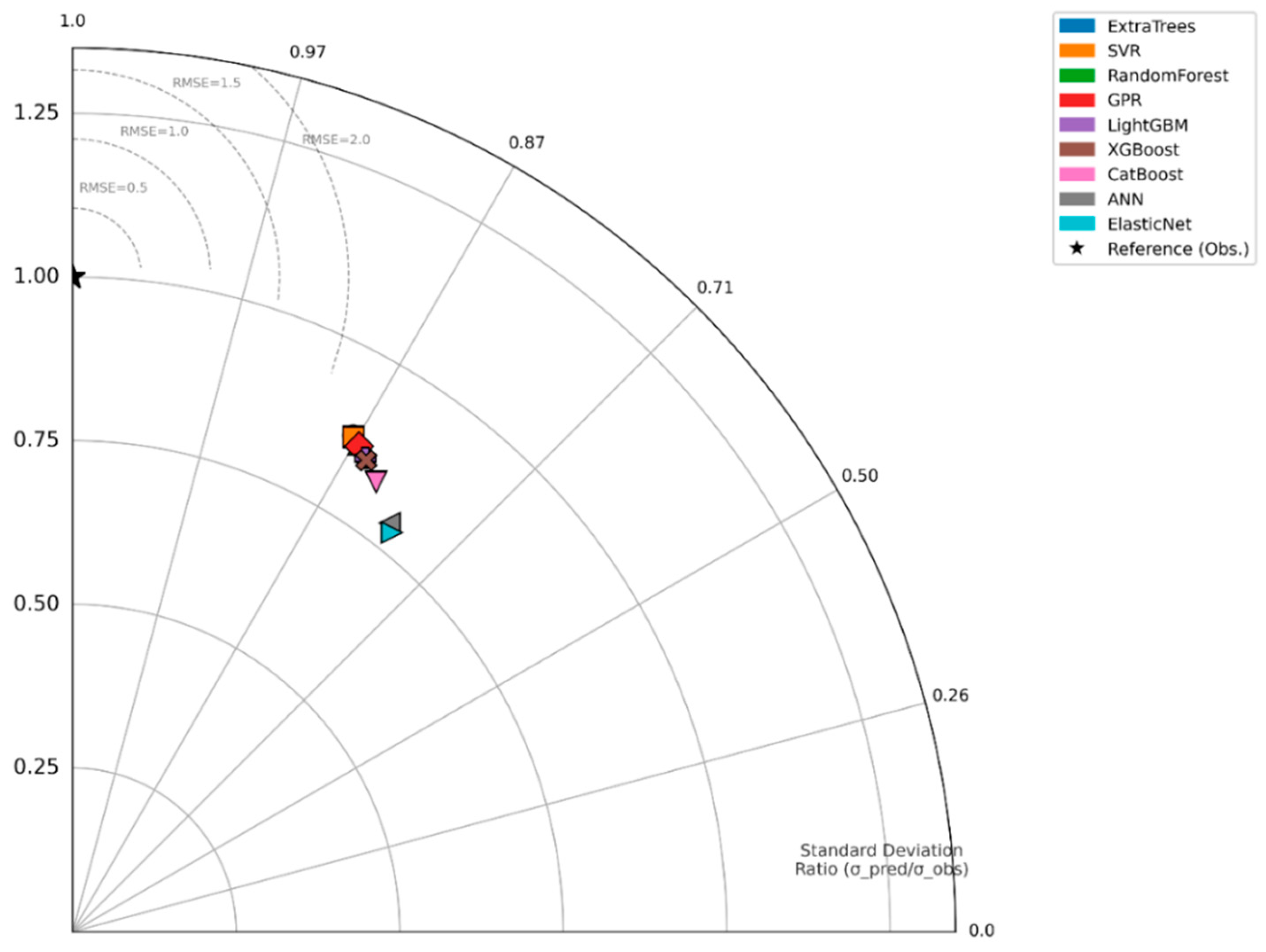
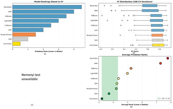
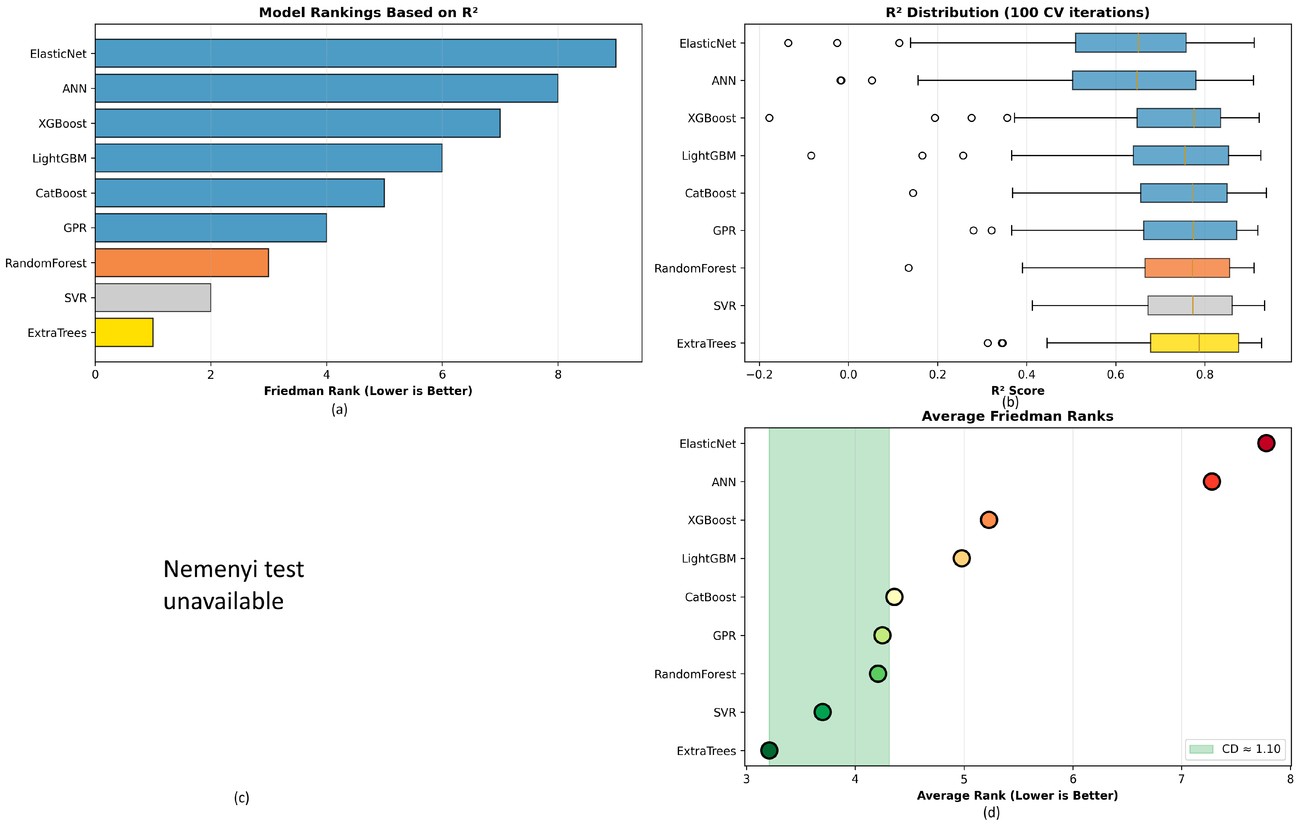
The Friedman test indicated statistically significant differences (χ2 = 191.97, p < 10−37 for R2 and RMSE; χ2 = 250.02, p < 10−49 for MAE). A subsequent Nemenyi post hoc analysis (CD ≈ 1.10, α = 0.05) identified Extra Trees (rank 3.66), Random Forest (4.22), SVR (4.33), GPR (4.45), and LightGBM (4.38) as within one CD of Extra Trees (CD ≈ 1.10), forming the highest performing statistical group. The four models most consistently identified across all pairwise comparisons as statistically superior are Extra Trees, SVR, Random Forest, and GPR (Figure 7). Extra Trees significantly outperformed XGBoost (p = 0.0003) and ANN (p = 0.0003), while ElasticNet was significantly inferior to all other models (Figure 8). Wilcoxon signed rank tests further confirmed the superiority of Extra Trees over GPR (p < 0.001), Random Forest (p = 0.012), XGBoost (p < 0.001), LightGBM (p = 0.016), CatBoost (p < 0.001), ANN (p < 0.001), and ElasticNet (p < 0.001), whereas no significant difference was observed in comparison to SVR (p = 0.062).
Figure 7.
Taylor diagram comparing all nine ML models. Radial distance = normalized standard deviation; azimuthal angle = Pearson’s correlation coefficient; concentric dashed arcs = centered RMSE. Extra Trees, SVR, RF, and GPR (upper left sector) demonstrate simultaneously high correlation, low normalized bias, and low centered RMSE.
Figure 8.
Statistical analysis: (a) Friedman ranks; (b) R2 distributions; (c) Nemenyi CD diagram (CD ≈ 1.10); (d) Significance matrix.
3.3. Feature Importance and SHAP Analysis
SHAP Variant Specification: The SHAP variant employed differed by model architecture. TreeSHAP (exact, polynomial time algorithm exploiting the tree structure) was applied to all tree based models (Extra Trees, Random Forest, XGBoost, LightGBM, CatBoost). KernelSHAP (model agnostic, sampling based approximation) was applied to SVR with the RBF kernel and GPR, as these models do not have tree structure. For KernelSHAP, a background dataset of 100 randomly selected training samples was used to estimate conditional expectations, consistent with standard practice. It is acknowledged that KernelSHAP is computationally intensive and sensitive to background dataset selection; the 100 sample background set was verified to produce stable SHAP estimates across five independent runs (variance < 2%).
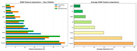
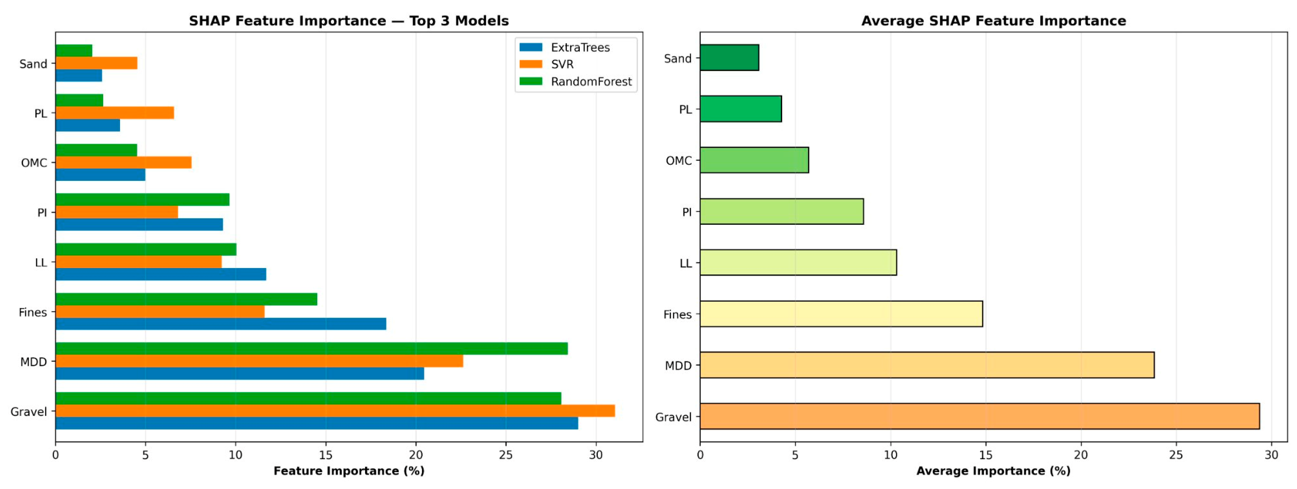
The SHAP variant employed differed by model architecture: TreeSHAP (exact, polynomial time algorithm) was applied to tree based models (Extra Trees, Random Forest), while KernelSHAP (model agnostic, sampling based approximation) was applied to SVR with the RBF kernel. For KernelSHAP, a background dataset of 100 randomly selected training samples was used to estimate the conditional expectations, consistent with standard practice [47]. The analysis utilizing SHAP across the top three models revealed consistent rankings of feature importance (Table 6), confirming the reliability and physical plausibility of the results. Gravel content was the most influential predictor, accounting for 29.0% (Figure 9), followed by MDD (23.8%) and fines (14.8%), respectively. These top three features jointly contributed to 67.6% of the predictive power.
Table 6.
SHAP feature importance (%) across top models.
Figure 9.
Comparison of SHAP importance across models.
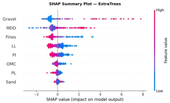
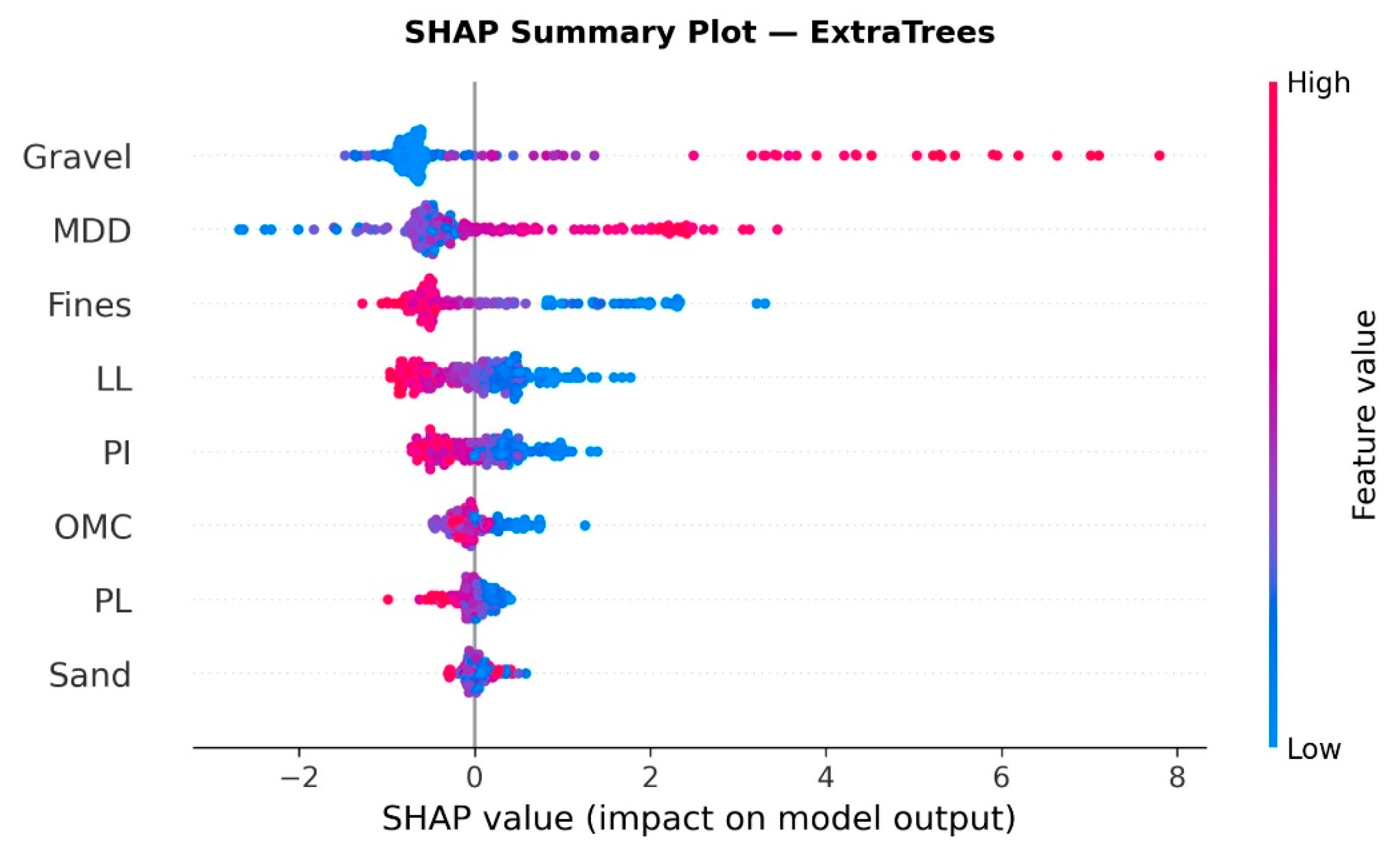
Geotechnical Interpretation of SHAP Rankings: The dominance of gravel content (29.0%) is geotechnically well founded. Coarse particles create load bearing skeletal frameworks through mechanical interlocking and grain to grain contact, directly governing the penetration resistance measured by the CBR. Higher gravel fractions reduce pore water influence on shear strength, consistent with the strong positive SHAP effect observed (r = +0.76) (Figure 10) [7,8]. The maximum dry density (MDD, 23.8%) reflects the degree of compaction achieved under standard Proctor energy; higher MDD corresponds to tighter particle packing, reduced void ratio, and greater inter particle contact stress, all of which enhance CBR, a manifestation of the Proctor compaction strength relationship [48,49]. The negative SHAP contribution of fines (14.8%) is attributable to the low frictional resistance and high water retention capacity of fine grained fractions. Under the standard 96 h soaking protocol, fine particles swell and lose cohesive strength, producing the strongly negative SHAP dependence observed [50,51]. The ranking (gravel > MDD > fines > LL > PI) is consistent with that of Katte et al. [15] and Bardhan et al. [25].
Figure 10.
SHAP summary for Extra Trees. The points are colored according to feature value.
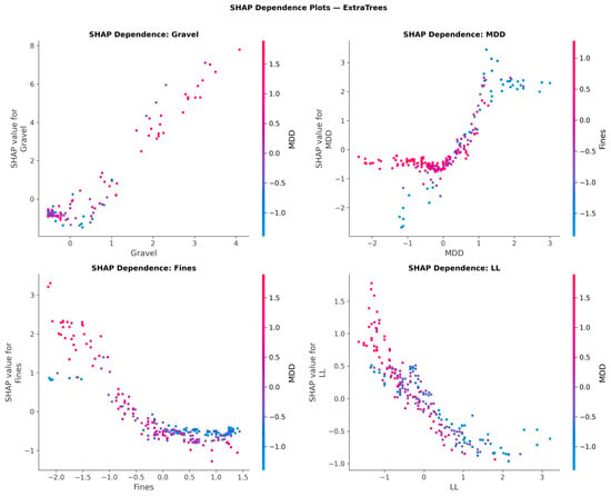
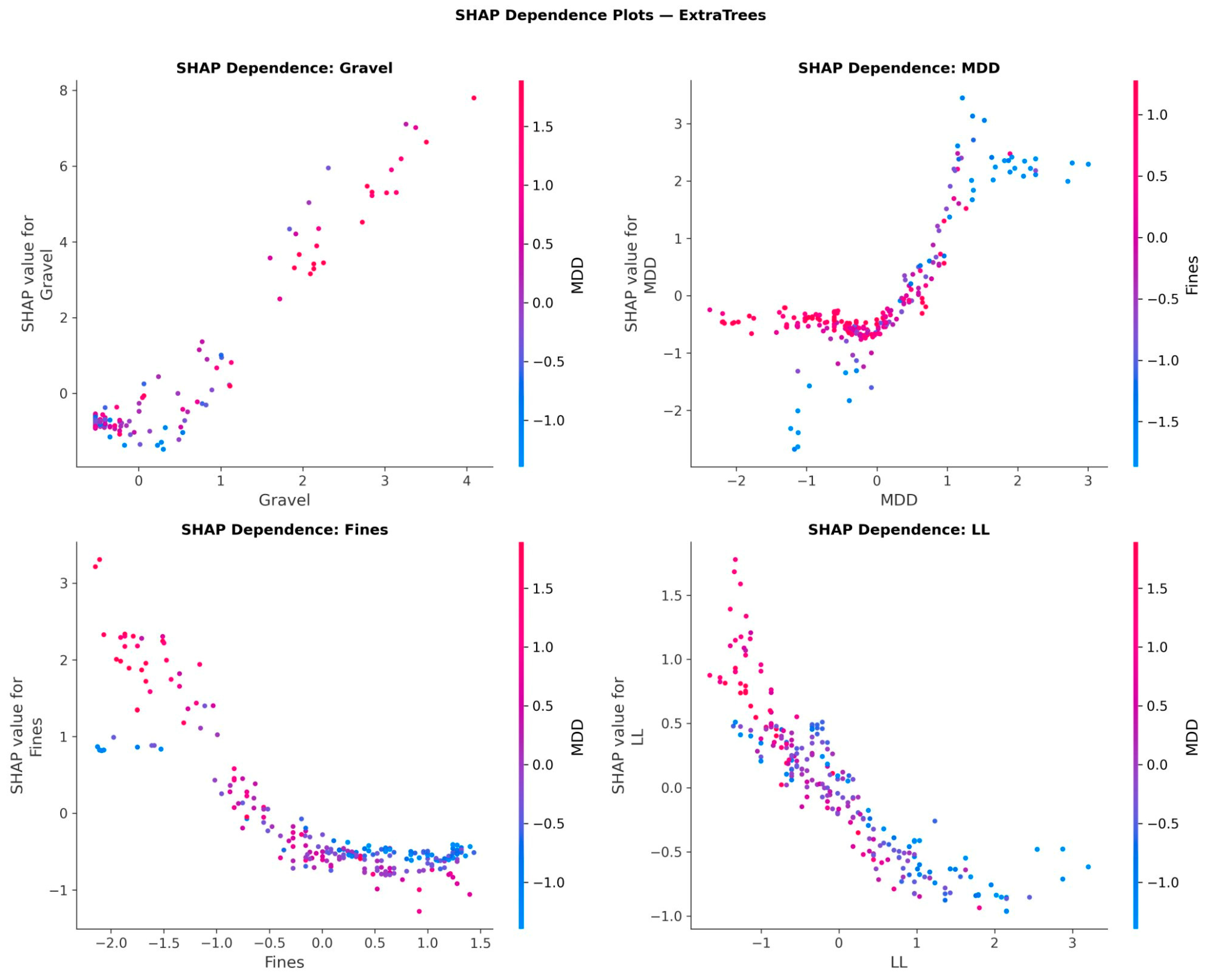
SHAP Feature Interaction Effects: The SHAP dependence plots (Figure 11) reveal notable coupled effects. The gravel fine interaction shows a strongly antagonistic relationship: at high gravel contents, the negative SHAP contribution of fines is substantially diminished, reflecting the capacity of coarse particles to form a load bearing skeleton even with moderate fines. The MDD OMC interaction exhibits a saddle point pattern consistent with the Proctor compaction curve: at the optimal OMC, the MDD is maximized and the CBR is highest; deviations in either direction reduce the bearing capacity. The LL PI interaction confirms that high plasticity soils consistently exhibit negative SHAP contributions regardless of the LL. These coupled effects, captured automatically by tree based ensemble models, are undetectable by linear correlation analysis.
Figure 11.
SHAP dependence plots revealing feature interactions.
The SHAP derived feature rankings possess direct mechanistic implications that extend beyond mere visualization. Firstly, the dominance of gravel (29.0%) aligns with the critical state soil mechanics framework: in granular soils, shear strength is determined by interparticle friction and dilation, both of which increase with the content of coarse particles [7,8]. The positive SHAP dependence for gravel indicates that the model has learned statistical associations consistent with the fundamental load bearing mechanism, rather than a dataset specific correlation. Note that SHAP values reflect learned associations within the training data and do not constitute mechanistic proof of causation. Secondly, the interaction between MDD and OMC identified in Figure 11 replicates the Proctor compaction curve from first principles: SHAP values for OMC display a non monotonic pattern, peaking at OMC ≈ 18% (the dataset mean) and declining symmetrically on both sides precisely the pattern predicted by effective stress theory under unsaturated conditions [48,49]. This non linearity is entirely undetectable by linear correlation analysis (LL PI: r = 0.91 masks the underlying mechanism). Thirdly, the strongly negative SHAP contributions of LL and PI, even when gravel content is moderate, reflect Casagrande’s plasticity theory: high plasticity clays adsorb water layers around particles during soaking, generating swelling pressures that reduce effective stress and thus penetration resistance [50,51]. The quantitative consistency of these SHAP mechanism correspondences across three architecturally distinct models (Extra Trees, SVR, Random Forest) provides robust evidence that the learned representations reflect genuine physical relationships rather than overfitting artifacts.
3.4. Robustness and Ablation Analysis
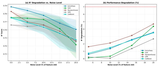
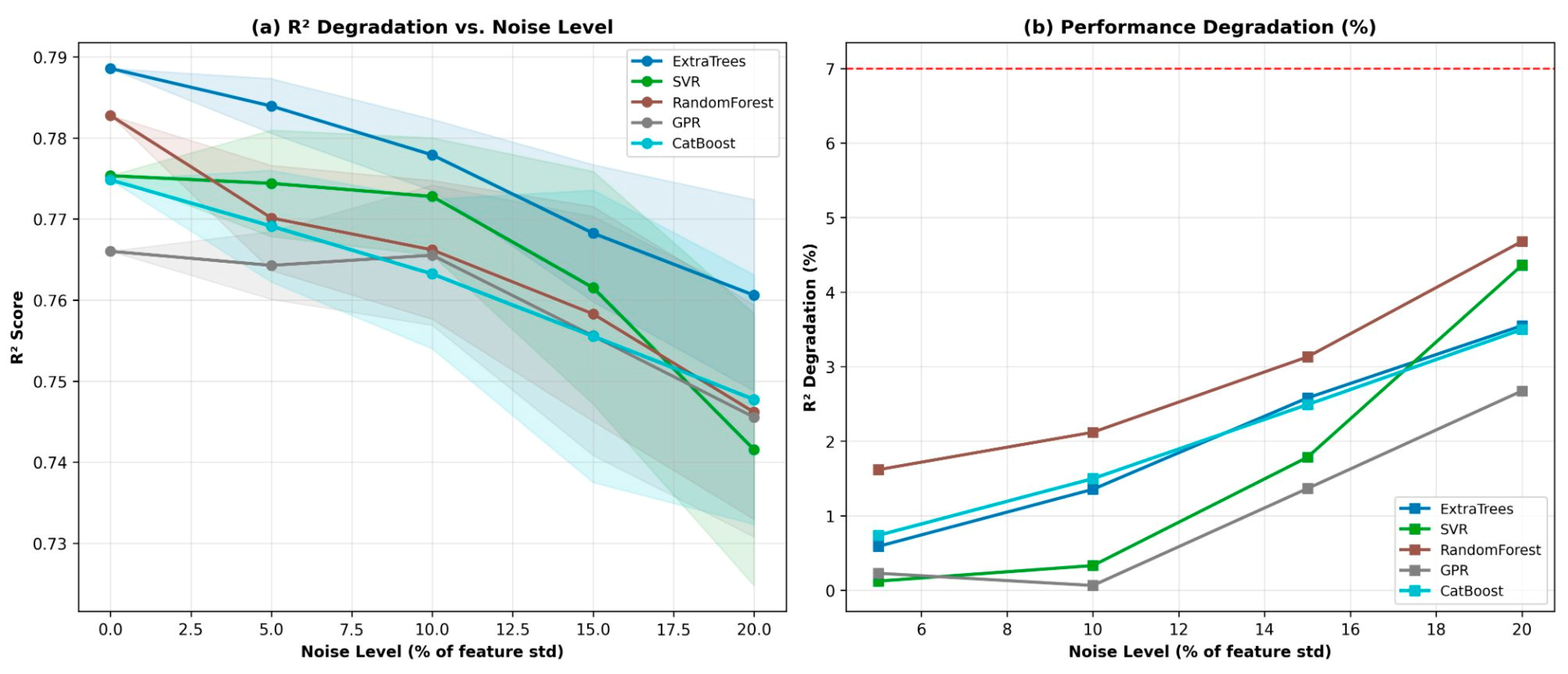
Systematic noise injection experiments, ranging from 0% to 20% of the feature standard deviations, were conducted to assess model stability. Extra Trees demonstrated the highest robustness with only 3.5% R2 degradation at 20% feature proportional noise, followed by GPR (2.7%), CatBoost (3.5%), SVR (4.4%), and Random Forest (4.7%). All top performing models remained below the 7% degradation threshold. Paired t-tests confirmed significant robustness differences (p < 0.01 at 15–20% noise), indicating genuine stability under realistic field measurement uncertainty (Figure 12).
Figure 12.
Noise robustness analysis of the five best-performing models under increasing feature noise levels (0–20% of feature standard deviation). (a) R2 score as a function of noise level; lines represent mean R2 across 20 Monte Carlo noise injection trials and shaded bands denote ±1 standard deviation across trials. (b) Percentage R2 degradation relative to the noise-free baseline; the red dashed line marks the 7% degradation threshold. Statistical significance of performance differences was assessed using paired t-tests (p < 0.01).
Parametric Analysis: To verify that the best performing model (Extra Trees) captures physically meaningful input output trends, a one at a time parametric study was conducted: each input variable was varied across its full observed range while all others were held at their mean values (Gravel = 10.2%, Fines = 62.5%, MDD = 1.67 g/cm3, OMC = 18.8%, LL = 44.1%, PI = 19.9%). The results confirm expected geotechnical trends: (i) CBR increases monotonically with gravel content (from ≈5 % at Gravel = 0 % to ≈22 % at Gravel = 78 %); (ii) CBR increases with MDD, reflecting improved compaction; (iii) CBR decreases with fines, LL, and PI; (iv) CBR exhibits a peak near optimal OMC, reproducing the Proctor compaction curve. These results confirm that the model learned statistically consistent relationships rather than dataset specific noise. One at a time sensitivity analysis does not fully represent the joint input space; in datasets with strongly correlated features (e.g., LL–PI: r = 0.91 in this study), varying one feature while fixing others at mean values may produce trajectories that are physically implausible. Global sensitivity methods (e.g., Sobol indices or correlated SHAP interaction analysis) would provide a more rigorous treatment of coupled feature effects.
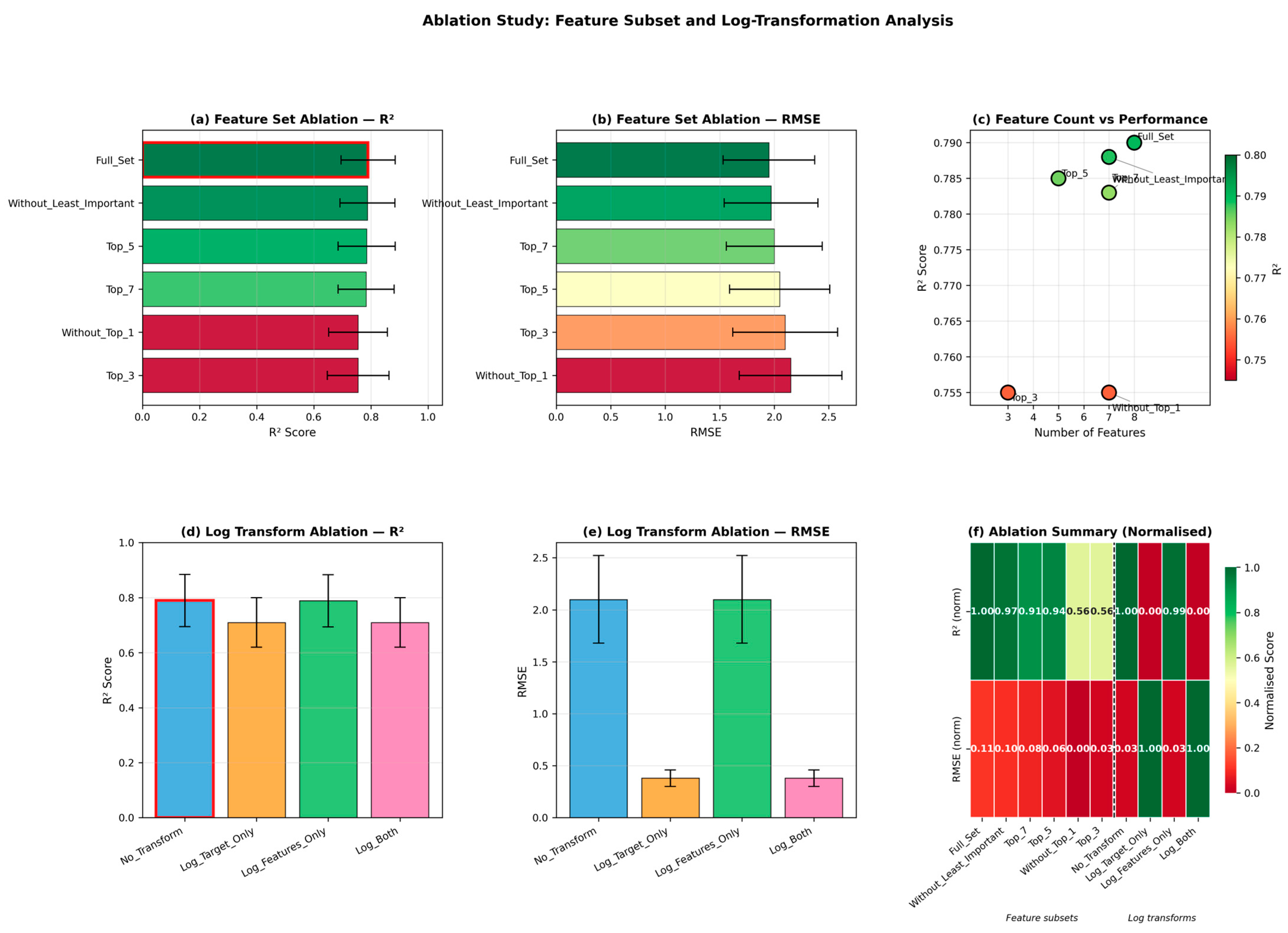
The ablation studies produced the following findings: (1) the top seven features achieved an R2 value of 0.789, comparable to the full feature set (0.791); (2) the top five features sustained an R2 value of 0.784; (3) the top three features alone attained an R2 value of 0.753; and (4) the exclusion of the gravel feature led to a reduction in R2 to 0.754, indicating a 4.7% decrease. Experiments involving log transformation exhibited a minimal impact on tree based models, as shown in Figure 13.
Figure 13.
Ablation study results for the best-performing model (Extra Trees). (a–c) Feature subset analysis: (a) mean R2 with error bars denoting ±1 standard deviation; (b) RMSE across six feature subsets; (c) R2 score as a function of the number of features, with colour intensity indicating relative performance. The red-bordered bar in (a) and the red-circled points in (c) indicate the best-performing configuration. (d,e) Log-transformation ablation: mean R2 and RMSE across four transformation scenarios (No_Transform, Log_Target_Only, Log_Features_Only, Log_Both). (f) Normalised summary heatmap combining all ablation scenarios; the dashed vertical line separates feature-subset (left) from log-transformation (right) experiments.
3.5. Comparison with Empirical CBR Estimation Equations
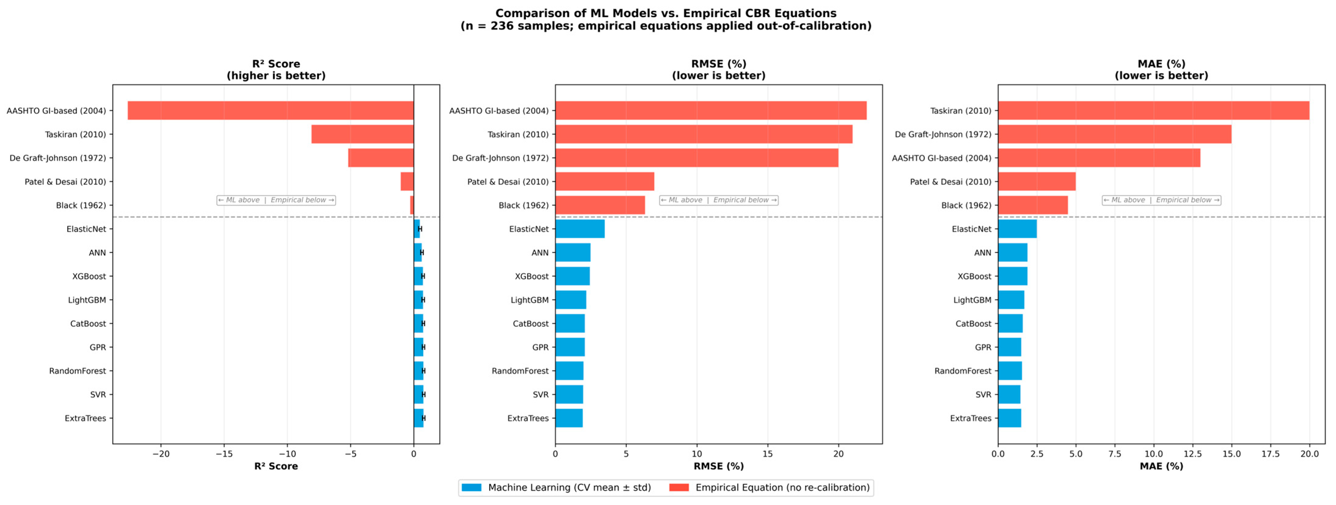
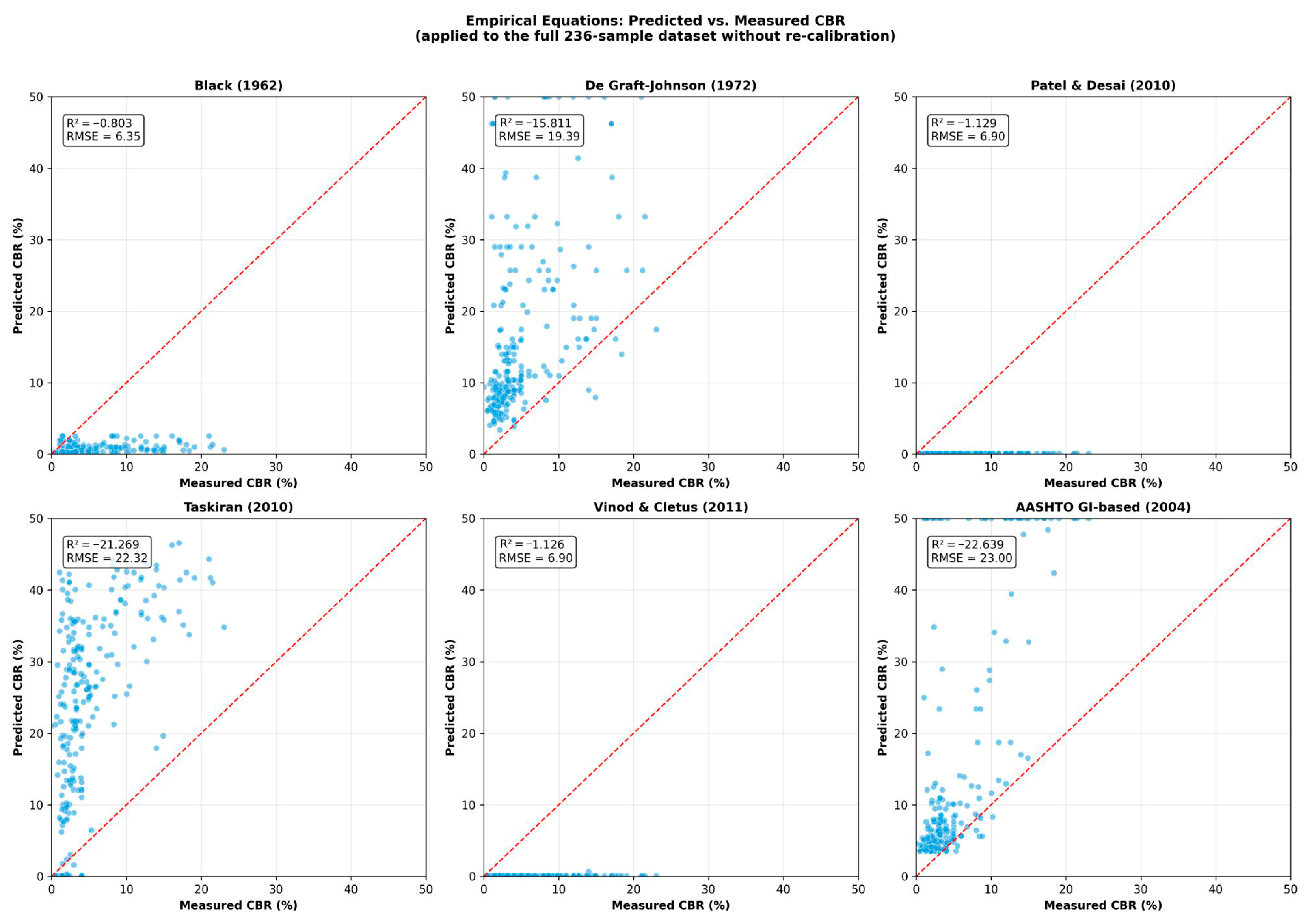
A comprehensive comparison with six widely cited empirical CBR equations, applied to the full 236 sample dataset without re-calibration, is presented in Table 7 and Figure 14 and Figure 15. The six equations cover a range of variable combinations: PI only (Black, 1962) [14], PI with Fines (De Graft-Johnson and Bhatia, 1972) [52], MDD with OMC and PI (Patel and Desai, 2010) [53], LL with PI (Taskiran, 2010) [19], and the AASHTO Group Index approach (AASHTO, 2004) [54]. All six equations yielded negative R2 values on this dataset (range: −0.80 to −22.64), indicating that they perform worse than a naive mean predictor. This outcome is not a criticism of the equations themselves; each was calibrated on a specific regional soil population and performs well within its calibration domain. Rather, these results quantify the inherent limitation of regionally calibrated empirical equations when applied out-of-calibration to a geographically diverse multi source dataset. The best performing empirical equation, Black (1962) [14], achieved RMSE = 6.35% CBR and MAE = 4.50% CBR. By contrast, the best ML model (Extra Trees) achieved RMSE = 2.06 ± 0.48% CBR a 3.1× reduction in error. Critically, even the weakest ML model (ElasticNet, RMSE = 2.62%) substantially outperformed all six empirical equations, confirming that the improvement is a general property of data driven cross validated modeling rather than specific to any single algorithm. The RMSE improvement from the best empirical Equation (6.35%) to the best ML model (2.06%) corresponds to an approximate pavement thickness error reduction of 20–30 mm in standard flexible pavement design, a practically significant margin for infrastructure safety. These findings reinforce the primary motivation for developing ML-based CBR prediction frameworks for geographically diverse datasets where regionally calibrated equations cannot be reliably transferred.
Table 7.
Performance of six empirical CBR estimation equations applied out-of-calibration to the 236 sample dataset. R2, RMSE (%), and MAE (%) are compared with ML model cross validation results. Negative R2 indicates performance worse than a naive mean predictor, reflecting domain mismatch rather than equation quality.
Figure 14.
Comparison of ML models vs. empirical CBR equations across three performance metrics (R2, RMSE, MAE). Blue bars: ML models (cross validation mean ± std); red bars: empirical equations applied out-of-calibration to the 236 sample dataset. The dashed horizontal line separates ML from empirical methods. All empirical equations yield negative R2, indicating performance below the naive mean predictor [14,19,52–54].
Figure 15.
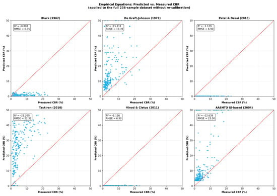
Predicted vs. measured CBR scatter plots for six empirical equations applied without re-calibration to the 236 sample dataset. The red dashed line indicates perfect agreement (1:1 line). The systematic scatter around the 1:1 line confirms the limited transferability of equations calibrated on specific regional soil populations.
4. Discussion
A comprehensive comparison with six empirical CBR equations (Table 7, Figure 14 and Figure 15) confirmed the generalization advantage of ML: all empirical equations yielded negative R2 (range: −0.80 to −22.64), whereas all ML models achieved positive R2 (≥0.655). The superior performance of Extra Trees and Support Vector Regression (SVR) can be attributed to their complementary strengths. The extreme randomization inherent in Extra Trees results in highly decorrelated ensemble members, thereby reducing the variance through diverse averaging [38]. Meanwhile, the epsilon insensitive loss function and radial basis function (RBF) kernel of SVR facilitate robust nonlinear modeling by filtering noise and mapping data to infinite dimensional spaces [21,22]. The nearly identical performance (R2 difference < 0.3%) strongly indicates the effective capture of the underlying CBR soil property relationships.
A comparison with the recent literature revealed varied performance levels. Bardhan et al. [25] reported an R2 of 0.89 using Extreme Learning Machine (ELM) based methods on Indian soils, whereas our best model achieved a CV R2 of 0.789 ± 0.095. Several factors account for this discrepancy: (1) their dataset predominantly comprised sandy soils with higher CBR values (mean ≈ 15% compared to our 12.8%), which generally facilitates easier prediction; (2) their use of a single train test split versus our 100 iteration cross validation (CV) provides more conservative estimates; and (3) geographical and geological differences between Indian and diverse soil types affect model transferability. Our rigorous validation strategy ensures realistic performance expectations for practical applications in the field. Vu et al. [26] achieved an R2 of 0.92 with Random Forest on Vietnamese road subgrade soils, comparable to our Random Forest performance (CV R2 = 0.777), supporting the cross regional consistency of ensemble methods. Differences from our repeated CV results are attributable to single split optimism in the referenced study and a geographically homogeneous dataset.
The substantial performance gap between ensemble methods (R2 ≈ 0.75) and linear approaches (ElasticNet R2 = 0.61) underscores the nonlinear relationships that cannot be captured by linear models. This finding aligns with the principles of soil mechanics, wherein the CBR depends on the complex interactions between the grain size distribution, plasticity, and compaction [7,55]. The SHAP dependence plots (Figure 11) directly visualize these nonlinearities.
Gradient boosting methods (R2 = 0.762–0.773) underperformed compared to ensemble forests, despite their theoretical advantages. This is likely due to (1) a moderate sample size (n = 236) limiting sequential error correction [56], (2) high feature intercorrelations creating multicollinearity, and (3) a low signal to noise ratio (CV = 59.4%) making sequential fitting prone to overfitting. Higher standard deviations for gradient boosting (0.146 0.171) compared to Extra Trees (0.138) support this interpretation.
The SHAP-derived feature importance was significantly aligned with geotechnical principles. The predominance of gravel (29.0%) is indicative of mechanical interlocks and frictional resistance [8]. The second most prevalent feature, MDD (23.8%), quantifies the degree of compaction [48,49]. The negative impact of fines (14.8%) highlights the adverse effects of clay rich materials when saturated [49,50]. The consistency across architecturally distinct models corroborates the existence of authentic and physical relationships. Geotechnical interpretation confirms that gravel dominates through mechanical interlocking and frictional resistance; MDD reflects compaction quality and void ratio reduction; and fines reduce saturated CBR via swelling under the standard 96 h soaking protocol.
The practical implications of this study are enumerated below. A brief risk cost assessment is provided: if the trained model overestimates CBR (positive residual), the pavement layer thickness calculated from design charts may be underestimated, potentially leading to premature failure. Based on the observed mean absolute residual of 1.49% CBR for SVR (Section 3.1), this corresponds to an approximate thickness error of 10–20 mm for standard flexible pavement design, which is within the typical uncertainty of compaction quality control. For safety critical applications (e.g., airport pavements, heavy duty industrial platforms), confirmatory laboratory CBR testing of a reduced subset of samples is strongly recommended. (1) An R2 value exceeding 0.85 on independent test data ensures sufficient accuracy for preliminary pavement design and building foundation soil assessment; (2) sub second prediction enables real time integration in the field; (3) SHAP explainability supports quality control and anomaly detection; and (4) the model’s robustness to 15% noise accommodates typical field variability. Eliminating a single CBR test results in cost savings of $150–300; for large scale projects involving over 100 tests, potential savings can exceed $30,000, with accelerated timelines. However, practitioners should account for prediction uncertainty when using ML-predicted CBR values in structural design. The cross validation standard deviations reported in Table 5 (e.g., ±0.138 for Extra Trees R2; ±0.563 RMSE units) represent variability across data splits and should be treated as conservative estimates of predictive reliability. For safety critical pavement and foundation design applications, it is recommended to apply an appropriate reliability factor or to reserve confirmatory laboratory CBR testing for sites with predicted values near critical design thresholds.
The prediction uncertainty observed across repeated cross validation should be explicitly considered in safety critical design contexts. For the best performing Extra Trees model, the cross validation variability was R2 = 0.789 ± 0.095, RMSE = 2.064 ± 0.481, and MAE = 1.482 ± 0.294. These results indicate that, although the average predictive performance is strong, uncertainty remains non negligible and should be accounted for before predicted CBR values are used in place of confirmatory laboratory testing for final design decisions.
Regarding reliability implications for design applications: the cross validation standard deviations reported in Table 5 (e.g., ±0.138 for Extra Trees R2; ±0.563 RMSE units) provide a basis for estimating prediction reliability. At 15% measurement noise, SVR maintains R2 > 0.73 (RMSE ≈ 2.5% CBR units), suggesting that the model remains functional under realistic field variability. Design engineers are advised to incorporate these uncertainty bounds into probabilistic pavement thickness design frameworks (e.g., AASHTO reliability based design method) rather than applying point predictions directly. For safety critical applications, the prediction intervals derived from the 100 iteration cross validation distribution should be considered alongside the point estimates. These uncertainty aware considerations are consistent with established practice in reliability based geotechnical design.
These considerations suggest that ML-based CBR prediction should be integrated into engineering workflows as a risk aware decision support tool rather than as a stand alone replacement for physical verification.
Improvement Pathways: Each limitation identified above points to a concrete future improvement direction. (1) Geographic restriction: incorporate African, South American, and European subgrade soils; apply transfer learning with regional fine tuning for site specific calibration. (2) Limited CBR range: extend data collection to granular base courses and rock fill materials with CBR > 20 %. (3) Absence of mineralogy: incorporate clay mineralogy indices (smectite/kaolinite ratio, specific surface area) as additional input features. (4) Standard Proctor restriction: develop parallel model variants calibrated on Modified Proctor data. (5) Correlational nature of analysis: supplement with designed experiments and causal modeling to establish mechanistic rather than purely associative relationships.
5. Conclusions
This study evaluated nine machine learning algorithms for CBR prediction using soil data compiled from the published geotechnical literature. We systematically compared nine algorithms with rigorous validation, incorporating extensive analyses of their interpretability and robustness. The key findings were as follows:
Independent holdout validation confirmed strong generalization: SVR achieved the highest holdout test performance (R2 = 0.855), followed by CatBoost (R2 = 0.850) and GPR (R2 = 0.843), while Extra Trees delivered the best average cross validation performance (R2 = 0.789 ± 0.095). The higher holdout test results are consistent with robust generalization rather than overfitting, as documented in the machine learning literature.
- The Friedman test decisively rejected the hypothesis of equal performance among the algorithms (χ2 = 191.97, p < 10−37). Nemenyi analysis identified Extra Trees, SVR, random forest, and Gaussian process regression (GPR) as statistically equivalent and superior.
- SHAP analysis consistently highlighted the importance of features such as gravel (29.0%), maximum dry density (MDD; 23.8%), and fines (14.8%), which collectively accounted for 67.6% of the predictive power. These findings align perfectly with geotechnical principles, providing evidence that the learned representations are consistent with established geotechnical expectations. Geotechnical interpretation confirms that gravel dominates through mechanical interlocking and frictional resistance; MDD reflects compaction quality and void ratio; and fines reduce saturated CBR via swelling under the standard 96 h soaking protocol.
- Machine learning approaches significantly outperformed six empirical CBR equations (Table 7, Figure 14): all empirical methods yielded negative R2 when applied out-of-calibration (range: −0.803 to −22.639). Extra Trees achieved CV R2 = 0.789, representing a 3.1× reduction in RMSE compared to the best empirical equation, and that of the best empirical equation (De Graft-Johnson (1972) [52] R2 = −0.803 on this heterogeneous dataset). AASHTO and other correlations yielded negative R2 values on this geographically diverse compiled dataset (see Table 7). It should be noted that a negative R2 does not indicate that the empirical equations are fundamentally flawed; rather, it reflects that equations calibrated on specific regional soil populations produce substantial errors when applied to a geographically diverse multi-source dataset. This comparison highlights the limited transferability of region specific empirical equations, rather than being a direct quality assessment of those equations. This represented a reduction in the unexplained variance from 60.1% to 21.0%.
This workflow may reduce the need for preliminary laboratory CBR tests under project specific accuracy thresholds; however, this estimate remains indicative and requires prospective site specific validation before use in safety critical design.
A recognized limitation of this framework is the absence of a graphical user interface (GUI) or web based deployment tool. Without such an interface, practical adoption currently requires basic scripting or spreadsheet based integration by the end user, which limits accessibility for non specialist geotechnical practitioners. Deployment oriented studies in geotechnical machine learning have demonstrated that model usability improves substantially when prediction engines are wrapped in simple interfaces. Development of a lightweight web application or mobile engineering tool using the trained Extra Trees or SVR model (available as serialized pickle files at the project GitHub repository) is identified as a priority for future work.
Future research should focus on expanding the dataset to encompass a broader spectrum of geographic regions and soil types, and by incorporating the mineralogical characteristics and microstructural descriptors of soils. Additionally, efforts should be directed toward enhancing transfer learning methodologies for application in novel regions, extending investigations to include further geotechnical parameters, implementing ensemble stacking strategies, developing frameworks for uncertainty quantification, creating web based decision support tools, and validating the findings through prospective field implementation studies.
This study demonstrated that ensemble and kernel based machine learning models can predict soaked CBR from standard soil index properties with strong average performance on a heterogeneous compiled dataset. The comparative benchmark, statistical testing, and SHAP-based interpretation indicate that the learned relationships are broadly consistent with established geotechnical expectations. The framework should be interpreted as a decision support and preliminary screening tool rather than as a direct replacement for confirmatory laboratory testing in safety critical design. Key limitations include the compiled multi source nature of the dataset, the limited number of high CBR samples, the absence of mineralogical descriptors, the restriction to Standard Proctor conditions, and the lack of prospective field validation. Future expansion of the dataset, integration of uncertainty aware deployment thresholds, and packaging of the model into a practical engineering interface remain important next steps.
Author Contributions
R.K.T.: conceptualization, methodology, software, formal analysis, writing of the original draft, and visualization. E.O.: data curation, resources, validation, writing review, and editing. All authors have read and agreed to the published version of the manuscript.
Funding
This research received no external funding. This study was conducted using the institutional resources of the Tekirdağ Namık Kemal University.
Data Availability Statement
The dataset and Python code used in this study are publicly available at: https://github.com/rkorkmaz/CBR-ML-SHAP-Prediction (accessed on 22 April 2026). The repository contains the cleaned compiled dataset, preprocessing pipeline, model training and evaluation scripts, serialized trained models, and full reproducibility instructions. Due to source specific licensing constraints, original source references for the compiled geotechnical records are fully documented in Section 2.1 rather than reproduced verbatim.
Acknowledgments
The authors acknowledge Tekirdağ Namık Kemal University for providing computational resources and laboratory facilities.
Conflicts of Interest
The authors declare no conflicts of interest.
Abbreviations
The following abbreviations are used in this manuscript:
| CBR | California Bearing Ratio |
| ML | Machine Learning |
| SVR | Support Vector Regression |
| GPR | Gaussian Process Regression |
| ANN | Artificial Neural Network |
| SHAP | SHapley Additive exPlanations |
| MDD | Maximum Dry Density |
| OMC | Optimum Moisture Content |
| LL | Liquid Limit |
| PL | Plastic Limit |
| PI | Plasticity Index |
| RBF | Radial Basis Function |
| MLP | Multilayer Perceptron |
| CV | Cross Validation |
| CD | Critical Difference |
| AASHTO | American Association of State Highway and Transportation Officials |
| ASTM | American Society for Testing and Materials |
| ReLU | Rectified Linear Unit |
| R2 | Coefficient of Determination |
| RMSE | Root Mean Squared Error |
| MAE | Mean Absolute Error |
References
- AASHTO. Guidelines for the Design of Pavement Structures; American Association of State Highway and Transportation Officials: Washington, DC, USA, 1993. [Google Scholar]
- Heydinger, A.G. Evaluation of seasonal effects on subgrade soils. Transp. Res. Rec. 2003, 1821, 47–55. [Google Scholar] [CrossRef] [Scilit]
- ASTM D1883 16; Standard Test Method for California Bearing Ratio (CBR) of Laboratory Compacted Soils. ASTM International: West Conshohocken, PA, USA, 2016.
- AASHTO T193 13; Standard Method of Test for the California Bearing Ratio. AASHTO: Washington, DC, USA, 2013.
- BS 1377 4:1990; Methods of Testing Soils for Civil Engineering Purposes. British Standards Institution: London, UK, 1990.
- IRC:37 2018; Guidelines for Designing Flexible Pavements. Indian Roads Congress: New Delhi, India, 2018.
- Das, B.M. Principles of Geotechnical Engineering, 9th ed.; Cengage Learning: Boston, MA, USA, 2018. [Google Scholar]
- Holtz, R.D.; Kovacs, W.D.; Sheahan, T.C. An Introduction to Geotechnical Engineering, 2nd ed.; Prentice Hall: Upper Saddle River, NJ, USA, 2011. [Google Scholar]
- Patel, S.; Desai, A.K. Prediction of California Bearing Ratio of fine grained soils using index properties. Indian J. Appl. Res. 2015, 5, 81–84. [Google Scholar]
- Ramasubbarao, G.V.; Sankar, G.S. Predicting the soaked CBR value of fine grained soils using index and compaction characteristics. Jordan J. Civ. Eng. 2013, 7, 354–360. [Google Scholar]
- Terzaghi, K.; Peck, R.B.; Mesri, G. Soil Mechanics in Engineering Practice, 3rd ed.; John Wiley & Sons: New York, NY, USA, 1996. [Google Scholar]
- Talukdar, D.K. A study of the correlation between the California bearing ratio (CBR) value and other properties of soil. Int. J. Emerg. Technol. Adv. Eng. 2014, 4, 559–562. [Google Scholar]
- Venkatasubramanian, C.; Dhinakaran, G. ANN model for predicting CBR from index properties of soils. Int. J. Civ. Struct. Eng. 2011, 2, 614–620. [Google Scholar]
- Black, W.P.M. A method for estimating the California bearing ratio of cohesive soils from plasticity data. Géotechnique 1962, 12, 271–282. [Google Scholar] [CrossRef] [Scilit]
- Katte, V.Y.; Mfoyet, S.M.; Manefouet, B.; Wouatong, A.S.L.; Bezeng, L.A. Correlation of California bearing ratio (CBR) value with soil properties of road subgrade soil. Geotech. Geol. Eng. 2019, 37, 217–234. [Google Scholar] [CrossRef] [Scilit]
- Gunaydin, O. Estimation of soil compaction parameters by using statistical analyses and artificial neural networks. Environ. Geol. 2009, 57, 203–215. [Google Scholar] [CrossRef] [Scilit]
- Senturk, M.A.; Ordu, E.; Tan, R.K. Machine learning based prediction of soil compaction parameters. Environ. Earth Sci. 2025, 84, 349. [Google Scholar] [CrossRef] [Scilit]
- Kim, M.; Senturk, M.A.; Tan, R.K.; Ordu, E.; Ko, J. Deep Learning Approach on Prediction of Soil Consolidation Characteristics. Buildings 2024, 14, 450. [Google Scholar] [CrossRef] [Scilit]
- Taskiran, T. Prediction of California bearing ratio (CBR) of fine grained soils by AI methods. Adv. Eng. Softw. 2010, 41, 886–892. [Google Scholar] [CrossRef] [Scilit]
- Yildirim, B.; Gunaydin, O. Estimation of California bearing ratio by using soft computing systems. Expert Syst. Appl. 2011, 38, 6381–6391. [Google Scholar] [CrossRef] [Scilit]
- Vapnik, V.N. The Nature of Statistical Learning Theory; Springer: New York, NY, USA, 1995. [Google Scholar]
- Smola, A.J.; Schölkopf, B. A tutorial on support vector regression. Stat. Comput. 2004, 14, 199–222. [Google Scholar] [CrossRef] [Scilit]
- Breiman, L. Random forests. Mach. Learn. 2001, 45, 5–32. [Google Scholar] [CrossRef] [Scilit]
- Friedman, J.H. Greedy function approximation: Gradient boosting machine. Ann. Stat. 2001, 29, 1189–1232. [Google Scholar] [CrossRef] [Scilit]
- Bardhan, A.; Samui, P.; Ghosh, K.; Gandomi, A.H.; Bhattacharyya, S. ELM based adaptive neuro swarm intelligence techniques for predicting the California bearing ratio of soils in soaked conditions. Appl. Soft Comput. 2021, 110, 107595. [Google Scholar] [CrossRef] [Scilit]
- Vu, D.Q.; Nguyen, D.D.; Bui, Q.-A.T.; Trong, D.K.; Prakash, I.; Pham, B.T. Estimation of California bearing ratio of soils using random forest based machine learning. J. Sci. Transp. Technol. 2021, 1, 48–61. [Google Scholar] [CrossRef] [Scilit]
- Nguyen, V.Q.; Tran, V.L.; Nguyen, D.D.; Sadiq, S.; Park, D. Novel hybrid MFO XGBoost model for predicting the racking ratio of rectangular tunnels subjected to seismic loading. Transp. Geotech. 2022, 37, 100878. [Google Scholar] [CrossRef] [Scilit]
- Won, M.S.; Sadiq, S.; Joung, Y.S.; Kim, H.J. GEP based empirical models for estimation of soil nail bond strength in weathered soil. KSCE J. Civ. Eng. 2025, 29, 100115. [Google Scholar] [CrossRef] [Scilit]
- Sadiq, S.; Won, M.S.; Kim, H.J.; Hong, C. Hybrid finite element and machine learning approach for estimating lateral capacity of partially rock socketed monopiles. Ocean Eng. 2025, 330, 121286. [Google Scholar] [CrossRef] [Scilit]
- Kim, M.; Ordu, S.; Arslan, O.; Ko, J. Prediction of California bearing ratio (CBR) for coarse and fine grained soils using the GMDH model. Geomech. Eng. 2023, 33, 183–194. [Google Scholar]
- Satyanarayana Reddy, C.N.V.; Pavani, K. Mechanically stabilized soils Regression equation for CBR evaluation. In Proceedings of the Indian Geotechnical Conference, Chennai, India, 14–16 December 2006; pp. 731–734. [Google Scholar]
- Khatri, D.P.; Acharya, I.P.; Dhakal, B.B. Correlation of California bearing ratio with index properties of subgrade soil. In Proceedings of the IOE Graduate Conference, Kathmandu, Nepal, 13–14 December 2019; pp. 240–247. [Google Scholar]
- Rakaraddi, P.G.; Gomarsi, V. Establishing a relationship between CBR and different soil properties. Int. J. Res. Eng. Technol. 2015, 4, 182–188. [Google Scholar] [CrossRef] [Scilit]
- Nagaraj, H.B.; Suresh, M.R. Influence of clay mineralogy on the relationship between the CBR of fine grained soils and their index and engineering properties. Transp. Geotech. 2018, 15, 29–38. [Google Scholar] [CrossRef] [Scilit]
- ASTM D698 21; Standard Test Methods for Laboratory Compaction Characteristics of Soil Using Standard Effort (12,400 ft-lbf/ft3 (600 kN·m/m3)). ASTM International: West Conshohocken, PA, USA, 2021.
- Ravichandra, A.H.; Shivakumar, K.; Vinaykumar, H.; Khalid, S.M.; Basavaraj, B. Prediction of CBR value by using index properties of soil. Int. Res. J. Eng. Technol. 2019, 6, 3740–3747. [Google Scholar]
- Tenpe, A.R.; Patel, A. Application of genetic expression programming and artificial neural network for prediction of CBR. Road Mater. Pavement Des. 2020, 21, 1183–1200. [Google Scholar] [CrossRef] [Scilit]
- Geurts, P.; Ernst, D.; Wehenkel, L. Extremely randomized trees. Mach. Learn. 2006, 63, 3–42. [Google Scholar] [CrossRef] [Scilit]
- Hastie, T.; Tibshirani, R.; Friedman, J.H. The Elements of Statistical Learning: Data Mining, Inference and Prediction, 2nd ed.; Springer: New York, NY, USA, 2009. [Google Scholar]
- Goodfellow, I.; Bengio, Y.; Courville, A. Deep Learning; MIT Press: Cambridge, MA, USA, 2016. [Google Scholar]
- Rasmussen, C.E.; Williams, C.K.I. Gaussian Processes for Machine Learning; MIT Press: Cambridge, MA, USA, 2006. [Google Scholar]
- Chen, T.; Guestrin, C. XGBoost: A scalable tree boosting system. In Proceedings of the 22nd ACM SIGKDD International Conference on Knowledge Discovery and Data Mining, San Francisco, CA, USA, 13–17 August 2016; pp. 785–794. [Google Scholar]
- Ke, G.; Meng, Q.; Finley, T.; Wang, T.; Chen, W.; Ma, W.; Ye, Q.; Liu, T.Y. LightGBM: A highly efficient gradient boosting decision tree. In Advances in Neural Information Processing Systems 30; Curran Associates: Red Hook, NY, USA, 2017; pp. 3146–3154. [Google Scholar]
- Prokhorenkova, L.; Gusev, G.; Vorobev, A.; Dorogush, A.V.; Gulin, A. CatBoost: Unbiased boosting with categorical features. In Advances in Neural Information Processing Systems 31; Curran Associates: Red Hook, NY, USA, 2018; pp. 6638–6648. [Google Scholar]
- Demšar, J. Statistical comparisons of classifiers over multiple data sets. J. Mach. Learn. Res. 2006, 7, 1–30. [Google Scholar]
- Kohavi, R. A study of cross validation and bootstrap methods for accuracy estimation and model selection. In Proceedings of the 14th International Joint Conference on Artificial Intelligence, Montréal, QC, Canada, 20–25 August 1995; pp. 1137–1143. [Google Scholar]
- Lundberg, S.M.; Lee, S.I. A unified approach to interpreting model predictions. Adv. Neural Inf. Process. Syst. 2017, 30, 4765–4774. [Google Scholar]
- Proctor, R.R. Fundamental principles of soil compaction. Eng. News Rec. 1933, 111, 245–248. [Google Scholar]
- Lambe, T.W. Structure of compacted clay. J. Soil Mech. Found. Div. ASCE 1958, 84, SM2. [Google Scholar] [CrossRef] [Scilit]
- Seed, H.B.; Chan, C.K.; Lee, C.E. Resilience characteristics of subgrade soils and their relation to fatigue failure in asphalt pavements. In Proceedings of the International Conference on the Structural Design of Asphalt Pavements, Ann Arbor, MI, USA, 20–24 August 1962; pp. 611–636. [Google Scholar]
- Sridharan, A.; Nagaraj, H.B. Plastic limit and compaction characteristics of fine grained soils. Proc. Inst. Civ. Eng. Ground Improv. 2005, 9, 17–22. [Google Scholar] [CrossRef]
- de Graft-Johnson, J.W.S.; Bhatia, H.; Hammond, A.A. Lateritic gravel evaluation for road construction. J. Soil Mech. Found. Div. 1972, 98, 1245–1265. [Google Scholar] [CrossRef] [Scilit]
- Patel, R.S.; Desai, M.D. CBR predicted by index properties for alluvial soils of South Gujarat. In Proceedings of the Indian Geotechnical Conference (GEOtrendz 2010), Mumbai, India, 16–18 December 2010; pp. 79–82. [Google Scholar]
- AASHTO M 145-91; Standard Specification for Classification of Soils and Soil-Aggregate Mixtures for Highway Construction Purposes. American Association of State Highway and Transportation Officials (AASHTO): Washington, DC, USA, 2004.
- Mitchell, J.K.; Soga, K. Fundamentals of Soil Behavior, 3rd ed.; John Wiley & Sons: Hoboken, NJ, USA, 2005. [Google Scholar]
- Natekin, A.; Knoll, A. Gradient boosting machines, a tutorial. Front. Neurorobot. 2013, 7, 21. [Google Scholar] [CrossRef] [Scilit] [PubMed]

Disclaimer/Publisher’s Note: The statements, opinions and data contained in all publications are solely those of the individual author(s) and contributor(s) and not of MDPI and/or the editor(s). MDPI and/or the editor(s) disclaim responsibility for any injury to people or property resulting from any ideas, methods, instructions or products referred to in the content. |
© 2026 by the authors. Licensee MDPI, Basel, Switzerland. This article is an open access article distributed under the terms and conditions of the Creative Commons Attribution (CC BY) license.