Numerical Simulation and Experimental Investigation of Welding Residual Stress in Tube-Sphere Welds of Welded Hollow Sphere Joint Grid Structures

Abstract

To investigate the distribution pattern and magnitude of residual stress at the weld toe of pipe-sphere connections in welded hollow sphere joints, the blind-hole method was employed to measure welding residual stress at both the spherical weld toe and pipe weld toe, yielding the magnitude and distribution characteristics of the residual stress. Additionally, the VISUAL-Environment finite element simulation software was utilized to obtain the temperature field, residual stress field, and residual stress distribution curves at the weld seam. The results indicate that welding residual stress in the entire welded hollow sphere joint exhibits both periodic and stochastic characteristics, with these two patterns showing good consistency. Meanwhile, finite element analysis results reveal the presence of both residual tensile and compressive stresses on the spherical surface and the connected pipe, with the welding residual stress maintaining a self-equilibrated state across the entire specimen. This study provides a foundational basis for subsequent research on the fatigue performance of grid structures with welded hollow sphere joints.

1. Introduction

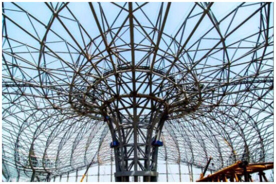
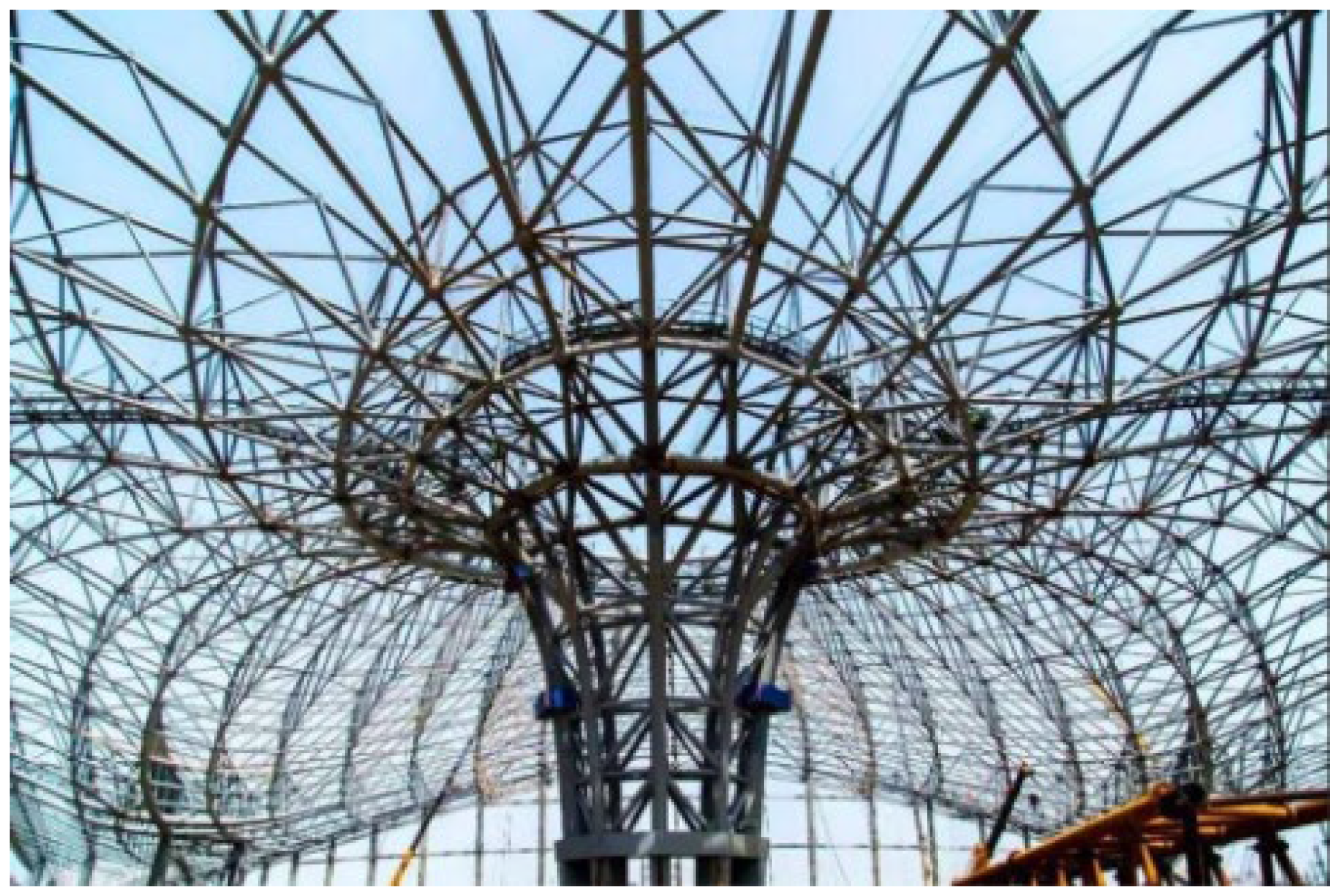
Grid structures have been extensively employed worldwide owing to their esthetic architectural appearance, reasonable mechanical performance, and adaptability to large-span structures, among other attributes [1,2]. As a form of spatial truss structure, members and joints serve as the core components of grid structures, where joints connect members to form a regular structural system. In comparison with other structural systems, grid structures are typically high-order statically indeterminate structures, characterized by three-dimensional force-bearing behavior, excellent integrity and stability, and high safety margins. They demonstrate superior seismic performance under both static and dynamic loads. Additionally, grid structures feature relatively uniform dimensional specifications, which facilitate manufacturing and on-site assembly [3]. A schematic of a grid structure is presented in Figure 1.

Figure 1. Welded hollow ball nodes for grids.

In grid structures, welded hollow spherical joints are the most extensively utilized joint type [4,5,6]. Since Professor Liu Xiliang from Tianjin University successfully developed the welded hollow spherical joint in 1965, it has evolved into the most fundamental joint form in China’s grid structures [7]. This joint is constructed by joining two hot-pressed hemispheres via butt welds to form a hollow sphere, followed by connecting steel pipe members to the hollow sphere using either butt welds or filet welds. Proper bevels are prefabricated on the steel pipes, which are then bonded to the welded hollow spherical joints through arc welding.

The complexity and randomness of welded structures are particularly pronounced under the influence of uncertainties inherent in welding processes. During welding, the coupling effect between localized non-uniform heating and cooling, as well as the temperature field within and adjacent to the weld, gives rise to a non-uniformly distributed residual stress field inside the welded component [8]. The presence of welding residual stress exerts varying degrees of influence on the structure itself and the resistance of welded joints to brittle fracture, stress corrosion cracking, and high-temperature creep cracking—with a particularly significant impact on the fatigue strength of steel structures [9]. Studies have demonstrated that the presence of welding residual tensile stress facilitates the propagation of fatigue cracks even in compression-loaded joints. Even under cyclic compressive loading, the residual tensile stress maintains cracks in an open state for all or part of the loading cycle [10]. Therefore, the quantitative evaluation of residual stress in practical engineering holds crucial significance for structural design.

From the perspective of damage mechanics, the residual stress induced during welding is essentially an initial form of damage, a locally non-uniform deformation and residual strain field introduced by thermo-mechanical coupling. This initial damage gradually evolves under cyclic loading, ultimately leading to fatigue cracking. Existing studies have demonstrated that welding damage (including welding residual stress and welding defects) is a critical factor influencing the fatigue life of welded joints in steel structures. Wang et al. proposed a coupled damage thermo-mechanical simulation method to systematically investigate the effect of welding residual stress on the fatigue life of welded plates and CHS X-joints. Their results showed that neglecting residual stress leads to a significant overestimation of high-cycle fatigue life [11]. In the study of interface damage between composite materials and concrete, Nerilli et al. systematically revealed the deterioration law of bond-slip performance at the GFRP bar–concrete interface under an alkaline environment and temperature effects through a combination of experimental and analytical approaches. Their damage analysis framework also provides certain reference value for research on welding damage in metal structures [12].

In recent years, sustained attention has been paid to the fatigue performance and residual stress issues of welded hollow spherical joints. Zhang et al. conducted constant-amplitude fatigue tests on welded hollow spherical joints, derived the S-N curves at the weld toes of the spheres, and revealed the stress distribution patterns and fatigue failure mechanisms of such joints under tensile conditions through finite element analysis [13]. Yan et al. performed 25 constant-amplitude and four variable-amplitude fatigue tests on tube-sphere joints and found that the hot spot stress concentration factor at the weld toes of the spheres ranged from 2.0550 to 4.8600. They further established a practical fatigue design method based on nominal stress amplitude and hot spot stress amplitude [14]. Qiu et al. investigated the mechanical behavior of welded hollow spherical joints under high temperatures in fire scenarios, and observed that as the heating temperature increased, the bearing capacity of the joints gradually decreased while their ductility gradually increased [15]. Additionally, the significant impact of welding residual stress on fatigue crack propagation has also been verified in welded joints of steel bridge decks. The study by Chen et al. showed that the fatigue life at the weld toe when considering welding residual stress was approximately half of that when residual stress was ignored, fully demonstrating the critical role of residual stress in fatigue assessment [16]. Bercelli et al. established a linear elastic fracture mechanics model that accounts for the initial residual stress field near the weld toe, based on X-ray stress analysis and thermoelastic stress analysis, further confirming the important influence of residual stress on the high-cycle fatigue performance of welded joints [17].

The analysis of welding residual stress encompasses experimental testing and numerical analysis; their combination enables the acquisition of more accurate residual stress distribution curves and values. However, experimental test results are inevitably subject to influences such as human error and environmental factors, meaning that results for the same component may vary under different testing conditions. Numerical simulation methods include the inherent strain method, thermo-mechanical analysis, and viscoelastic analysis, among others. Thermo-mechanical analysis can track the entire welding thermal process, allowing for the real-time acquisition of the welding temperature field and stress-deformation field [18]. This paper thus employs this theory to perform numerical simulations of welding residual stress in components.

Currently, most studies on welding residual stress in welded hollow spherical joints rely on numerical simulation and analysis via finite element software such as VISUAL-Environment (Version 15.0), ANSYS, and ABAQUS, with relatively limited experimental investigation [19,20,21,22,23]. The determination of residual stress in welded structures has primarily focused on components like steel plates and angle steels, while research on curved-surface structures (e.g., spheres and tubes) remains scarce. The stress states at different locations on a spherical surface exhibit variations; during testing, measurements are mainly targeted at residual stress hot spots. Hot spots serve as the initiation sites of fatigue cracks, and for welded structures with sound welding quality, hot spots are mostly located at weld toes. Therefore, the distribution and measurement of welding residual stress at hot spots of tube-sphere welds holds significant importance.

This study takes the widely applied welded hollow spherical joints in grid structures as the research object. The temperature field and residual stress field of the entire component are obtained via simulation using VISUAL-Environment software. Additionally, the blind-hole method is employed to measure and analyze the welding residual stress at the tube-sphere weld of the welded hollow spherical joints, thereby deriving the distribution law of the residual stress.

2. Experimental Investigation

2.1. Measurement and Material Properties

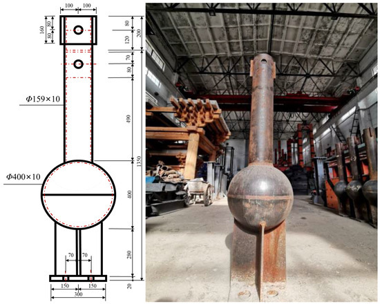
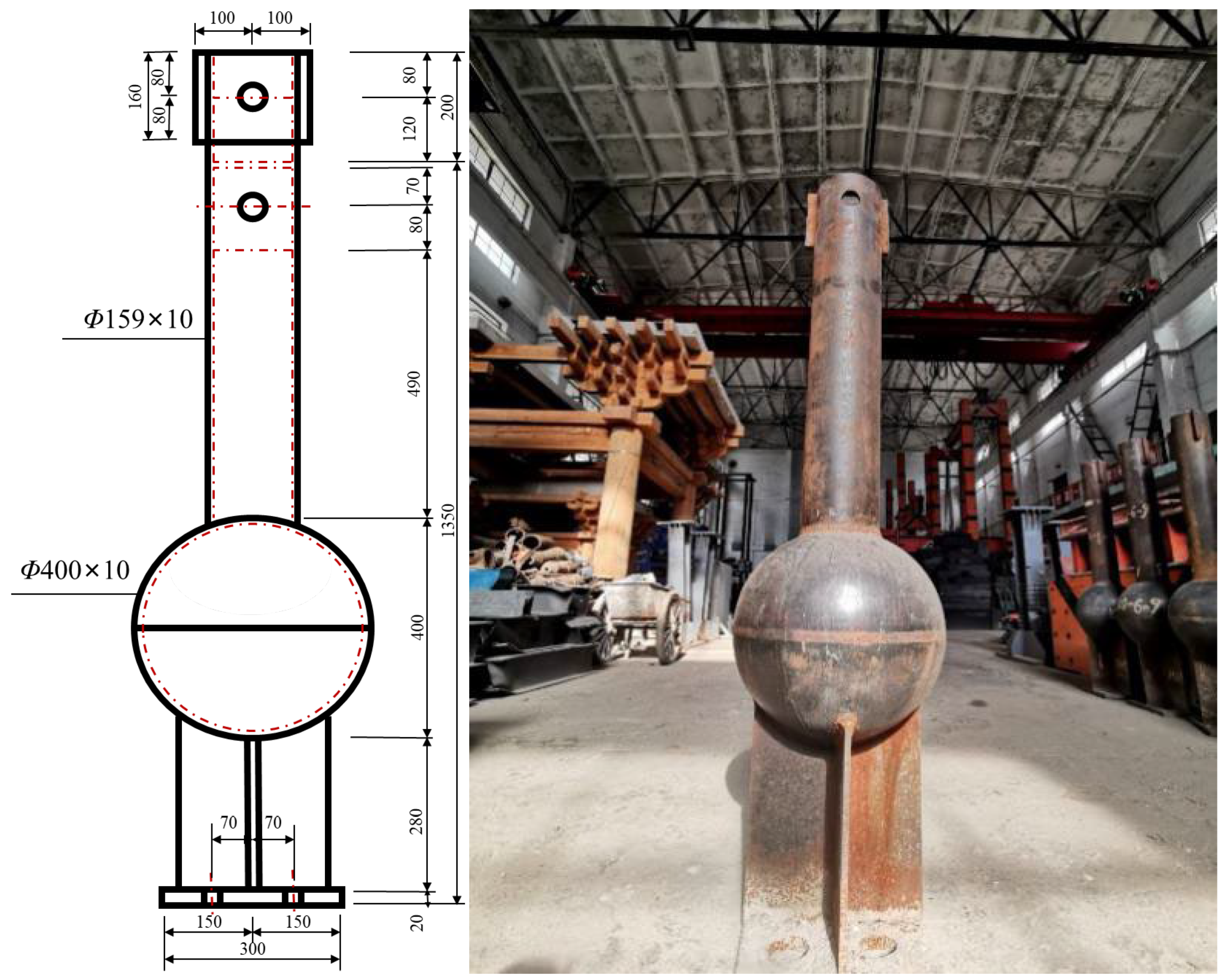
Test specimens GQ1-1, GQ1-2, and GQ1-3 are three parallel specimens of welded hollow spherical joints with identical dimensions, as shown in Figure 2. All specimens were fabricated from Q235B structural steel, with the following nominal material properties: elastic modulus E = 2.06 × 10⁵ MPa and Poisson’s ratio μ = 0.33. Specimen dimensions and welding parameters are summarized in Table 1.

Figure 2. Welded hollow spherical joints.

Table 1. Welded hollow ball node specimens.

Number	Welded Ball Specifications (mm)	Tube Specification (mm)	Pipe Ball Connection
GQ1	D400 × 10	Φ159 × 8	Bevel welding
GQ2	D400 × 10	Φ159 × 8	Bevel welding
GQ3	D400 × 10	Φ159 × 8	Bevel welding

2.2. Instrumentation Layout

Weld residual stresses near the weld toe are typically high in magnitude and constitute a critical location for fatigue crack initiation. To accurately characterize the residual stress distribution across the spherical joint surface and adjacent pipe surface, measurement points are strategically placed in the vicinity of the weld toe, where stress gradients are steepest and peak values occur. This targeted arrangement ensures a faithful representation of the actual residual stress state at the weld toe.

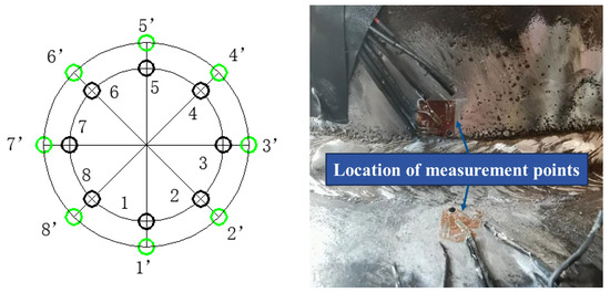
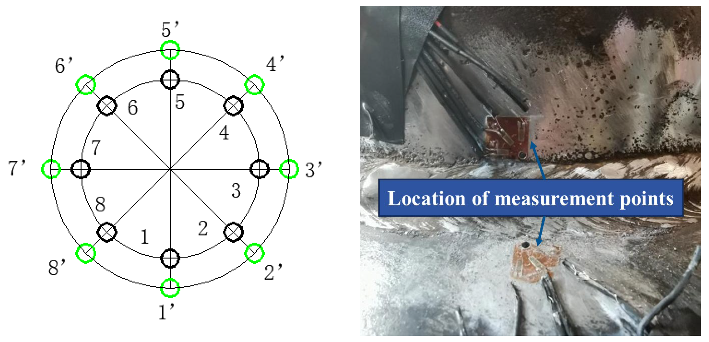
Each specimen features a welded joint, with eight measurement points on the spherical surface numbered 1′ to 8′ and eight on the tubular surface numbered 1 to 8, yielding a total of 16 measurement points per specimen. The blind-hole method is a destructive testing technique, precluding repeated measurements at the same location. The repeatability of this study is ensured through two approaches: cross-validation of results from eight circumferentially symmetric measurement points on the same specimen, and hole spacing as a critical experimental parameter governing measurement accuracy—smaller spacing increases the mechanical interference between adjacent blind holes, thereby compromising the integrity of residual stress release and introducing systematic error. As per ASTM E837 [24], the center-to-center distance between adjacent holes will exceed 5–8 times the hole diameter to ensure valid stress relaxation behavior. The precise spatial coordinates of all measurement points are detailed in Figure 3.

Figure 3. Layout of measurement points on the spherical and tubular surfaces.

2.3. Experimental Methodology and Instrumentation

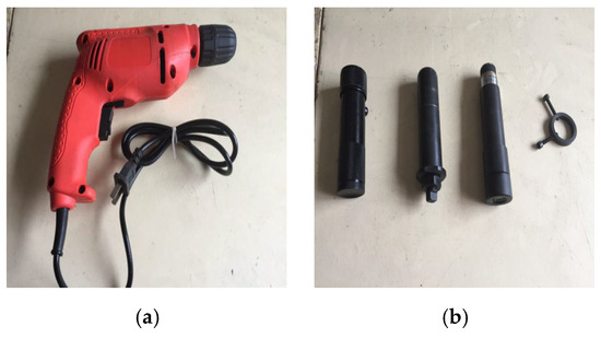
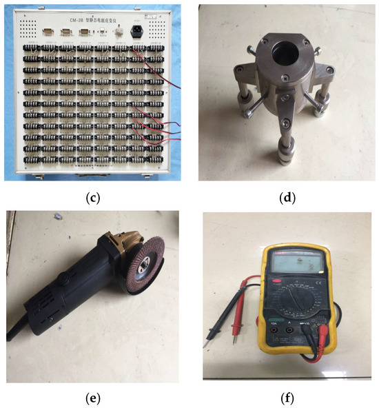
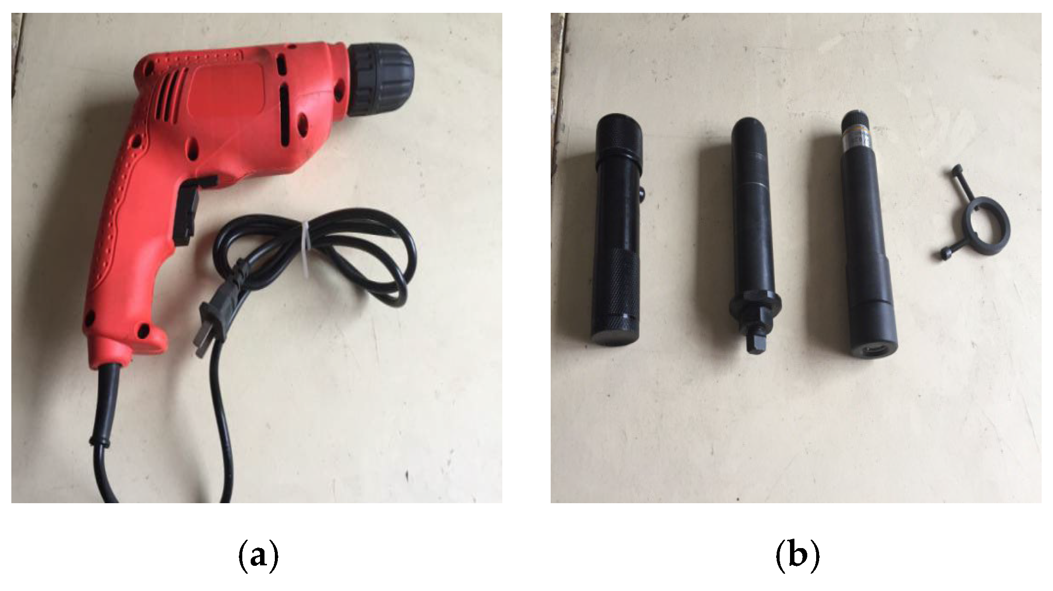
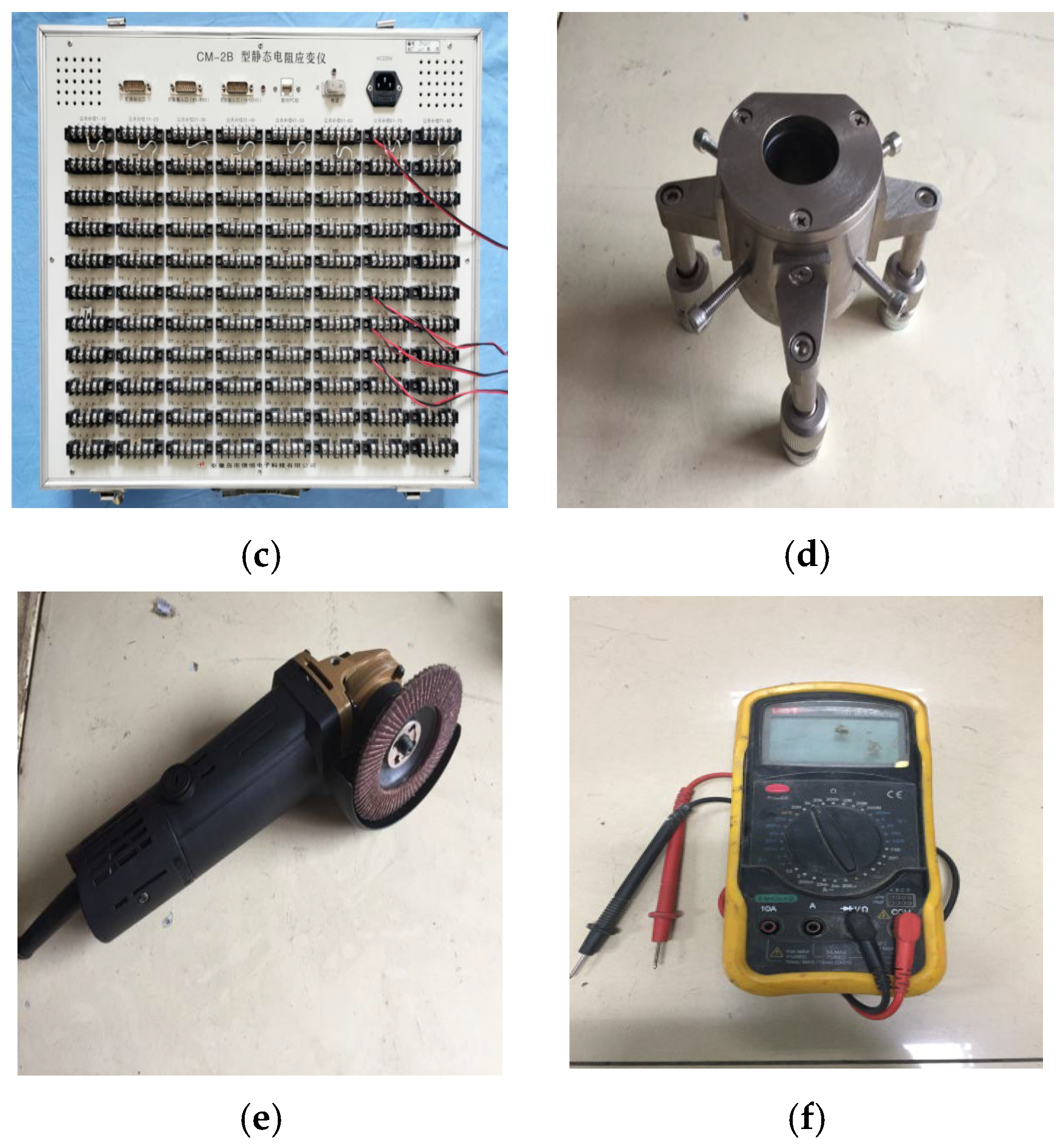
Residual welding stresses are measured using the blind-hole drilling method. The experimental setup comprises a CM-2B TCP-channel electrostatic resistance strain gauge (Beijing Shengzhen United High-Tech Research Institute, Beijing China), a ZS-IIA precision drilling device (Zhangjiakou Xuanhua Mingda Zhengyu Drilling Machinery Co., Ltd., Zhangjiakou China), and a three-element rosette strain gauge (model BX120-2CA), with a nominal resistance of 119.8 ± 0.1 Ω and a gauge factor of 2.08 ± 1%. A standard twist drill bit (diameter φ1.5 mm) is employed to produce blind holes of 1.5 mm diameter and 2 mm depth. All instrumentation is shown in Figure 4. The test environment is 20 ± 2 °C, with a relative humidity of no more than 60%.

Figure 4. Test equipment. (a) ZS-IIA drilling device, (b) ZS-IIA drilling device, (c) CM-2B TCP static strain measurement and analysis system, (d) drill pedestal, (e) angle grinder, and (f) a multimeter.

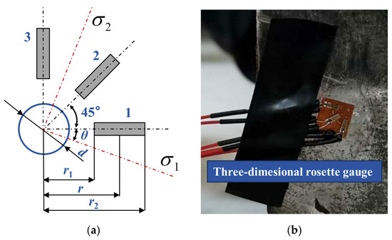
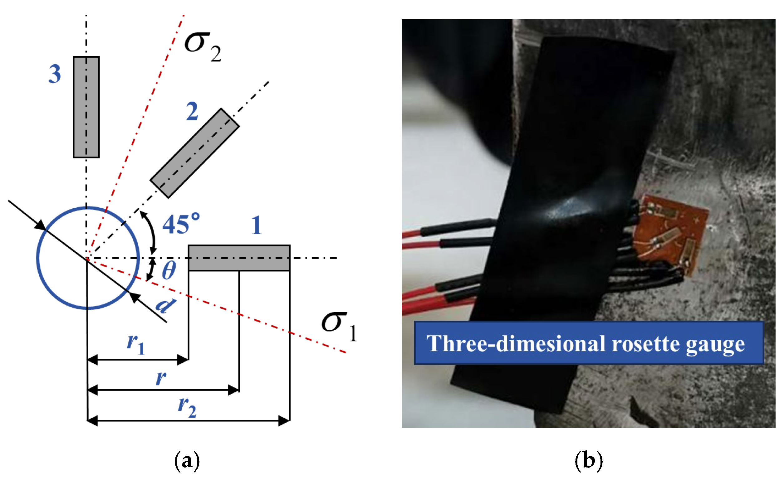
Given the unknown principal stress directions of welding residual stresses, a triaxial strain rosette with 45° and 90° orientations was employed in the experiment. The schematic of the strain rosette is illustrated in Figure 5a, while the actual drilling positions for the strain rosettes are presented in Figure 5b.

Figure 5. Blind-hole drilling locations for strain relief measurement: (a) theoretical strain gauge rosette orientation and coordinate system; (b) actual placement of the strain rosette on the specimen surface.

2.4. Fundamental Principle of the Blind-Hole Drilling Method

Three-directional strain rosettes (Figure 5a) are employed to measure the strain values of three orthogonal strain components (ε₁, ε₂, and ε₃) both before and after blind-hole drilling. The computational schematic is shown in Figure 6.

Figure 6. Calculation of residual stress in blind-hole method.

Prior to drilling, the relationship between the original welding residual stresses (σ_ρ, σ_ρ, τ_ρθ) at the measurement point and the residual principal stresses (σ₁, σ₂) is expressed by Equation (1):

$$\begin{array}{l}{\sigma }_{\rho }={\sigma }_1{\cos }^2\theta +{\sigma }_2{\sin }^2\theta \\ {\sigma }_{\theta }={\sigma }_1{\sin }^2\theta +{\sigma }_2{\cos }^2\theta \\ {\tau }_{\rho \theta }=\left({\sigma }_2-{\sigma }_1\right)\sin \theta \cdot \cos \theta \end{array}.$$

(1)

Through mathematical transformation, the following expression is derived:

$$\begin{array}{l}{\sigma }_{\rho }={\displaystyle \frac{1}{2}}\left({\sigma }_2+{\sigma }_1\right)+{\displaystyle \frac{1}{2}}\left({\sigma }_2-{\sigma }_1\right)\cos 2\theta \\ {\sigma }_{\theta }={\displaystyle \frac{1}{2}}\left({\sigma }_2+{\sigma }_1\right)-{\displaystyle \frac{1}{2}}\left({\sigma }_2-{\sigma }_1\right)\cos 2\theta \\ {\tau }_{\rho \theta }={\displaystyle \frac{1}{2}}\left({\sigma }_2-{\sigma }_1\right)\sin 2\theta \end{array}.$$

(2)

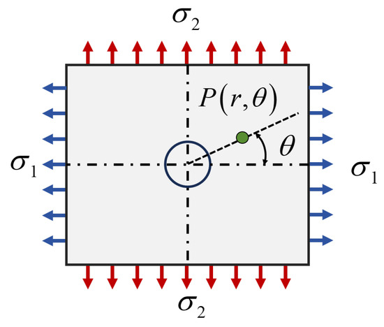
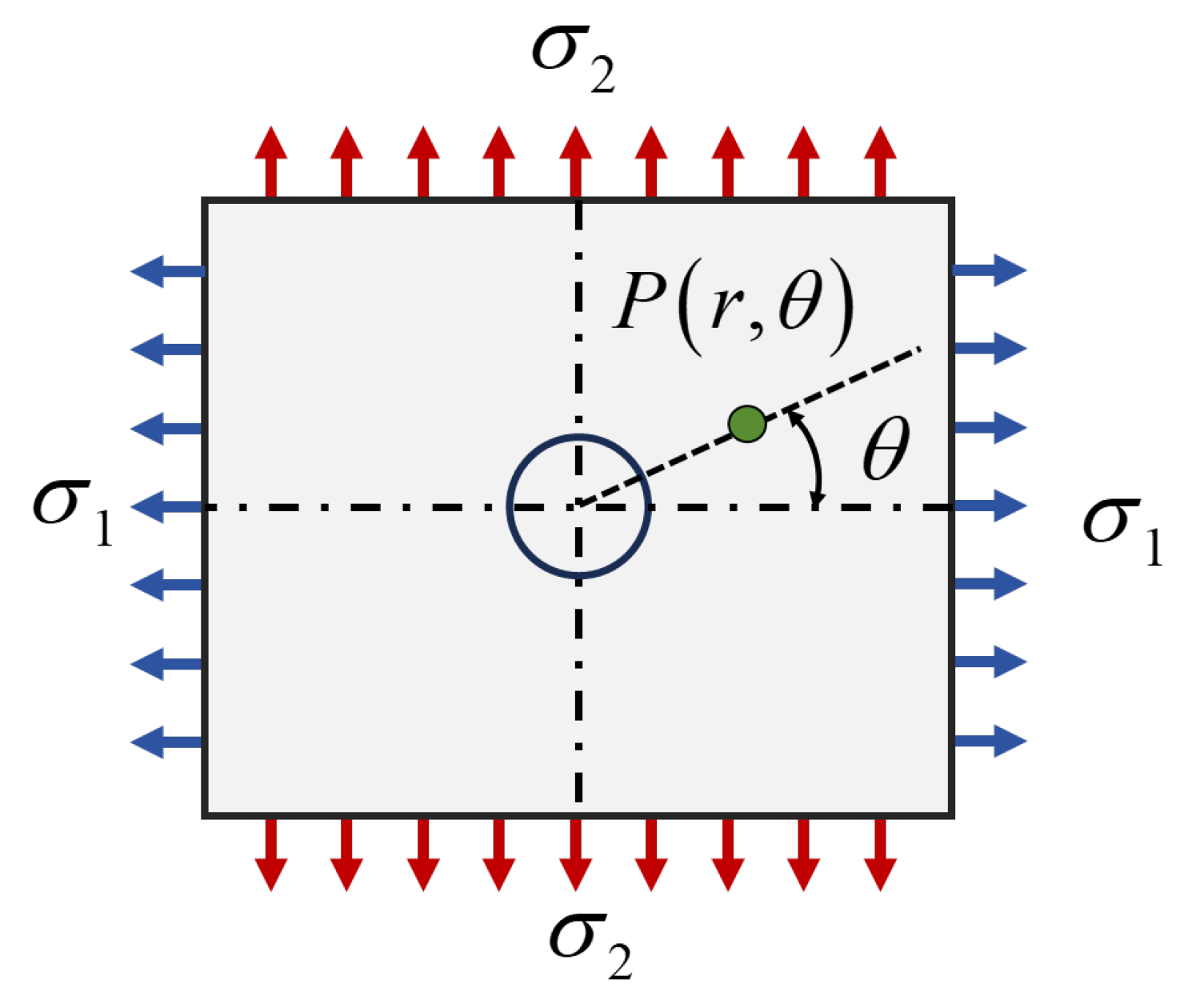
Upon drilling a small hole with radius a, the welding residual stress at the measurement point is instantaneously released. According to the theory of stress concentration around a circular hole in elasticity, this scenario is equivalent to applying uniform forces σ₁ and σ₂ around the hole perimeter. The stress state at the strain gauge position is thus given by:

$$\begin{array}{l}{\sigma }_{\rho 1}={\displaystyle \frac{1}{2}}\left({\sigma }_2+{\sigma }_1\right)\left(1-{\displaystyle \frac{a^2}{r^2}}\right)+{\displaystyle \frac{1}{2}}\left({\sigma }_2-{\sigma }_1\right)\left(1-{\displaystyle \frac{a^2}{r^2}}\right)\left(1-{\displaystyle \frac{3a^2}{r^2}}\right)\cos 2\theta \\ {\sigma }_{\theta 1}={\displaystyle \frac{1}{2}}\left({\sigma }_2+{\sigma }_1\right)\left(1+{\displaystyle \frac{a^2}{r^2}}\right)-{\displaystyle \frac{1}{2}}\left({\sigma }_2-{\sigma }_1\right)\left(1+{\displaystyle \frac{3a^4}{r^4}}\right)\cos 2\theta \\ {\tau }_{\rho \theta 1}={\displaystyle \frac{1}{2}}\left({\sigma }_2-{\sigma }_1\right)\left(1-{\displaystyle \frac{3a^4}{r^4}}+{\displaystyle \frac{2a^2}{r^2}}\right)\sin 2\theta \end{array}$$

(3)

The stress variation before and after drilling is thus expressed as:

$$\begin{array}{l}{\sigma }_{\rho }={\sigma }_{\rho 1}-{\sigma }_{\rho 0}={\displaystyle \frac{\left({\sigma }_2+{\sigma }_1\right)}{2}}\left(1-{\displaystyle \frac{a^2}{r^2}}\right)+{\displaystyle \frac{\left({\sigma }_2-{\sigma }_1\right)}{2}}\left(1-{\displaystyle \frac{a^2}{r^2}}\right)\left(1-{\displaystyle \frac{3a^2}{r^2}}\right)\cos 2\theta \\ {\sigma }_{\theta }={\sigma }_{\theta 1}-{\sigma }_{\theta 0}={\displaystyle \frac{\left({\sigma }_2+{\sigma }_1\right)}{2}}\cdot {\displaystyle \frac{a^2}{r^2}}-{\displaystyle \frac{\left({\sigma }_2-{\sigma }_1\right)}{2}}\cdot {\displaystyle \frac{3a^4}{r^4}}\cos 2\theta \\ {\tau }_{\rho \theta 1}={\tau }_{\rho \theta 1}-{\tau }_{\rho \theta 0}=-{\displaystyle \frac{\left({\sigma }_2-{\sigma }_1\right)}{2}}\left(-{\displaystyle \frac{3a^4}{r^4}}+{\displaystyle \frac{2a^2}{r^2}}\right)\sin 2\theta \end{array}$$

(4)

In accordance with the generalized Hooke’s law [25]:

$$\begin{array}{l}{\epsilon }_{\rho }={\displaystyle \frac{1}{E}}\left({\sigma }_{\rho }-\mu {\sigma }_{\theta }\right)\\ {\epsilon }_{\theta }={\displaystyle \frac{1}{E}}\left({\sigma }_{\varphi }-\mu {\sigma }_{\theta }\right)\end{array},$$

(5)

where E represents the elastic modulus of the material and μ represents the Poisson’s ratio of the material.

Upon substituting Equations (4) and (5), the radial release strain at point P is obtained as:

$${\epsilon }_{\rho }={\displaystyle \frac{1}{E}}\left\{{\displaystyle \frac{\left({\sigma }_2+{\sigma }_1\right)}{2}}\left[\left(-1-\mu \right)\cdot {\displaystyle \frac{a^2}{r^2}}\right]+{\displaystyle \frac{\left({\sigma }_2-{\sigma }_1\right)}{2}}\cdot \left[3\left(1+\mu \right){\displaystyle \frac{a^4}{r^4}}-{\displaystyle \frac{4a^2}{r^2}}\right]\cos 2\varphi \right\}.$$

(6)

Transform the radial release strain into a relational expression that depends solely on the principal stresses σ₁, σ₂, and the angle θ between the principal stress and the reference axis:

$$\begin{array}{l}A=-{\displaystyle \frac{1+\mu }{2}}\cdot {\displaystyle \frac{a^2}{r^2}}\\ B={\displaystyle \frac{1}{2}}\left[3\left(1+\mu \right){\displaystyle \frac{a^4}{r^4}}-{\displaystyle \frac{4a^2}{r^2}}\right]\end{array},$$

(7)

Then, the radial strain at point P is transformed to:

$${\epsilon }_{\rho }={\displaystyle \frac{A}{E}}\left({\sigma }_2+{\sigma }_1\right)+{\displaystyle \frac{B}{E}}\left({\sigma }_2-{\sigma }_1\right)\cos 2\theta .$$

(8)

Through mathematical formula derivation (where A and B represent strain release coefficients), stress σ is inferred from strain ε via inversion:

$$\left\{\begin{array}{l}{\sigma }_{1,2}={\displaystyle \frac{{\epsilon }_1+{\epsilon }_3}{4A}}\mp {\displaystyle \frac{1}{4B}}\sqrt{{\left({\epsilon }_1-{\epsilon }_3\right)}^2+{\left(2{\epsilon }_2-{\epsilon }_1-{\epsilon }_3\right)}^2}\\ \tan 2\theta ={\displaystyle \frac{2{\epsilon }_2-{\epsilon }_1-{\epsilon }_3}{{\epsilon }_3-{\epsilon }_1}}\end{array}\right.,$$

(9)

where σ₁ and σ₂ denote the major and minor in-plane principal residual stresses, respectively, θ represents the orientation angle of the major principal stress relative to the reference axis (as defined in Figure 6), A and B are the experimentally calibrated strain release coefficients specific to the rosette geometry and material system, and ε₁, ε₂, and ε₃ are the measured strain increments along the 0°, 45°, and 90° grid directions of the rectangular rosette, respectively. Once σ₁ and σ₂ are determined, the radial and circumferential components of the residual stress at each measurement point are obtained via elastic coordinate transformation, implemented using Equation (10):

$$\left\{\begin{array}{l}{\sigma }_{\rho }={\displaystyle \frac{1}{2}}\left({\sigma }_1+{\sigma }_2\right)+{\displaystyle \frac{1}{2}}\left({\sigma }_1-{\sigma }_2\right)\cos 2\theta \\ {\sigma }_{\theta }={\displaystyle \frac{1}{2}}\left({\sigma }_1+{\sigma }_2\right)-{\displaystyle \frac{1}{2}}\left({\sigma }_1-{\sigma }_2\right)\cos 2\theta \\ {\tau }_{\rho \theta }={\displaystyle \frac{1}{2}}\left({\sigma }_1-{\sigma }_2\right)\sin 2\theta \end{array}\right.\hspace{1em},$$

(10)

where σ_ρ represents radial stress, σ_θ represents cyclic stress, and τ_ρθ represents shear stress.

2.5. Determination of the Strain Relief Coefficients

The strain relief coefficients A and B are determined through a combination of analytical calculation and experimental calibration. The two governing equations for their derivation are as follows.

(1) The strain relief coefficients are calculated using the conventional analytical expression given in Equation (11):

$$\left\{\begin{array}{c}A=-{\displaystyle \frac{1+\mu }{2E}}\cdot {\displaystyle \frac{a^2}{r^2}}\\ B={\displaystyle \frac{1}{2E}}\left[3\cdot (1+\mu )\cdot {\displaystyle \frac{a^4}{r}}-{\displaystyle \frac{4a^2}{r^2}}\right]\end{array}\right..$$

(11)

The experimentally measured strain is substituted into Equation (11) to compute the strain relief coefficients:

$$\begin{array}{l}A=-0.1135\times {10}^{-6}/\mathrm{MPa}\\ B=-0.3294\times {10}^{-6}/\mathrm{MPa}\end{array}.$$

(2) The Kirsch theoretical solution, grounded in the through-hole strain release coefficient, incorporates the dimensions of the strain gauge. This solution is applicable to the calculation of the strain release coefficient for through-hole cases, as expressed in Equation (12):

$$\left\{\begin{array}{c}A=-{\displaystyle \frac{1+\mu }{2E}}\cdot ({\displaystyle \frac{d^2}{4r_1{r}_2}})\\ B={\displaystyle \frac{d^2}{2E{r}_1{r}_2}}\left[-1+{\displaystyle \frac{1+\mu }{4}}\cdot {\displaystyle \frac{d^2(r_1+r_1{r}_2+r_2^2)}{4r_1^2{r}_2^2}}\right]\end{array}\right..$$

(12)

For the blind-hole method, Saint-Venant’s principle implies that strain relaxation becomes depth-independent beyond a critical hole depth. Empirical and numerical studies indicate that when the depth-to-diameter ratio (h/d) falls within the range of 1.0–1.5, the measured strain release coefficient stabilizes and converges toward the value predicted by Kirsch’s analytical solution for an infinite plate with a through-hole. In this study, h/d = 1.33, within the validated stability range, thereby justifying the use of Kirsch’s solution as a theoretically grounded approximation for the strain release coefficient.

The experimentally measured strain increments are substituted into Equation (4) to compute the through-hole strain release coefficient:

$$\left\{\begin{array}{c}A=-0.11875\times {10}^{-6}/\mathrm{MPa}\\ B=-0.34260\times {10}^{-6}/\mathrm{MPa}\end{array}\right..$$

Most conventional blind-hole residual stress measurement protocols adopt Kirsch’s analytical solution, originally derived for through-hole relaxation, as the theoretical basis for determining the strain release coefficients. Comparative experimental and numerical studies confirm that, under standardized testing conditions, the resulting coefficients exhibit close agreement with those obtained from dedicated blind-hole calibration.

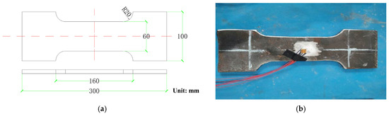
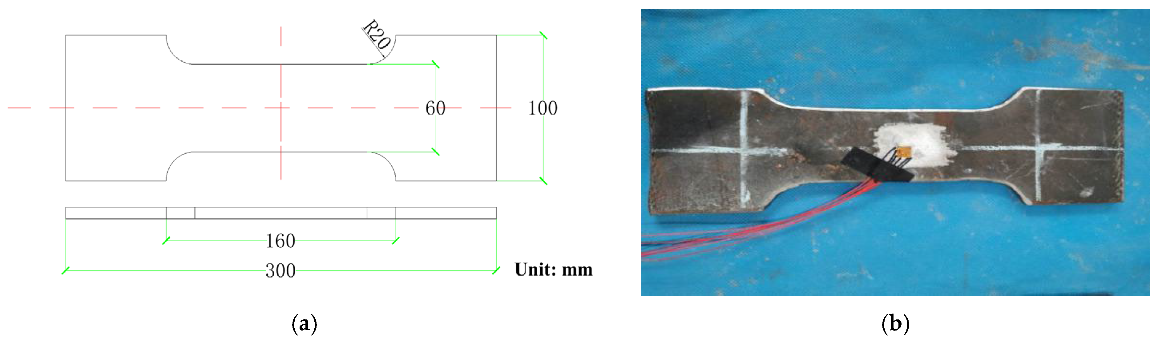
Three sets of calibration tests are conducted (BD1, BD2, BD3), all using Q235B steel identical to the base material. A 90° bidirectional strain rosette is placed at the same location on each specimen, and drilling is performed at the center of the strain rosette in accordance with the blind-hole method. The calibration dimensions and strain rosette layout are detailed in Figure 7. The experimentally determined strain relief coefficients A and B are summarized in Table 2.

Figure 7. Calibration geometry and strain rosette layout: (a) dimensional drawing; (b) actual component photograph.

Table 2. Calibration test for determining the strain relief coefficients A and B.

No.	Calibrated Stress /MPa	Release Strain ε1/με ε3/με		A Test Value (106/MPa)	B Test Value (106/MPa)	A Average (106/MPa)	B Average (106/MPa)	A (106/MPa)	B (106/MPa)
BD1	30	−15	7	−0.1333	−0.3666			−0.1259	−0.3525
	50	−28	10	−0.18	−0.38	−0.1425	−0.3584
	70	−31	15	−0.1143	−0.3286
BD2	30	−13	6	−0.1167	−0.3167
	50	−26	12	−0.14	−0.38	−0.1284	−0.3584
	70	−35	17	−0.1285	−0.3785
BD3	30	−12	7	−0.0833	−0.3167
	50	−25	12	−0.13	−0.37	−0.1068	−0.3408
	70	−31	16	−0.1071	−0.3357

A comparison between theoretical and experimental values shows the following: the theoretical value of strain release coefficient A is −0.11875 × 10⁻⁶ MPa, with an experimental value of −0.1259 × 10⁻⁶ MPa (relative error = 5.6%), and the theoretical value of strain release coefficient B is −0.3426 × 10⁻⁶ MPa, with an experimental value of −0.3525 × 10⁻⁶ MPa (relative error = 2.8%). It is evident that the experimental results exhibit good agreement with the theoretical analysis and are close to the theoretical solution. Thus, the strain release coefficients of the strain gauges in this experiment are determined as:

$$\left\{\begin{array}{c}A=-0.11875\times {10}^{-6}/\mathrm{MPa}\\ B=-0.34260\times {10}^{-6}/\mathrm{MPa}\end{array}\right..$$

2.6. Experimental Procedure

The experimental procedure can be divided into three parts: drilling, alignment, and strain acquisition

a. Tool alignment and optical centering

(1) The drilling jig is positioned on the surface of the welded hollow spherical member and secured magnetically. The base leveling screws are adjusted to co-locate the drill axis with the geometric center of the strain rosette, while ensuring the drill axis remained normal to the local tangent plane at the measurement site.

(2) A calibrated stereo microscope (magnification ×20) is mounted in its dedicated sleeve and is inserted into the jig. The jig height and microscope focus are fine-tuned to maximize orthogonality between the microscope optical axis and the sphere’s local surface; the positioning snap ring is then tightened to lock the assembly.

(3) The microscope crosshairs are centered over the target rosette. A full 360° rotation of the microscope confirmed concentricity: persistent alignment of the crosshair center with the rosette center throughout rotation verified that the intended drill path will be normal to the sphere’s tangent plane at the measurement point, ensuring accurate stress relaxation geometry. This optical verification step is shown in Figure 8.

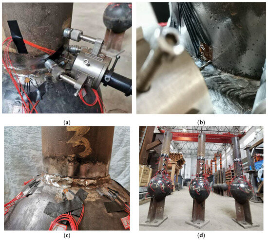
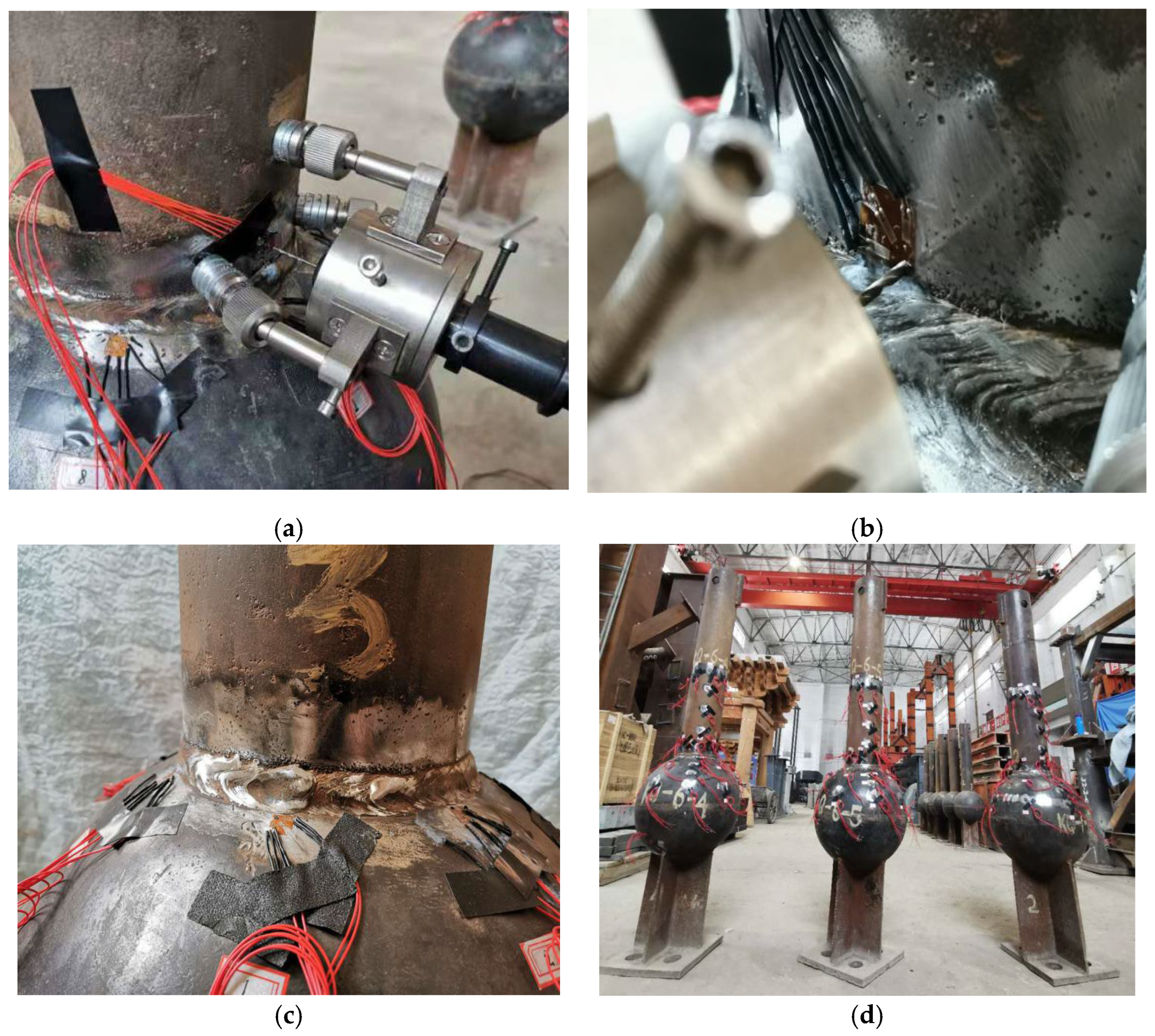
Figure 8. Blind-hole drilling sequence: (a) drilling jig installation; (b) hole drilling; (c) close-up view of rosette centering; (d) overall experimental setup.

(4) The positioning snap ring is loosened, the microscope is removed, and the static resistance strain gauge is re-zeroed immediately prior to drilling.

b. Blind-hole drilling and strain measurement

(1) The Φ1.5 mm twist drill is installed in the drill sleeve and secured. The sleeve is carefully seated into the jig base. A depth control spacer (2.00 mm total thickness, comprising stacked 1.5 mm and 0.5 mm precision-ground blocks) is inserted to limit hole depth; the positioning snap ring is tightened, and the spacer is withdrawn. The strain gauge is then re-zeroed.

(2) Drilling commences using a low-speed, variable-frequency hand drill (rotational speed: 300–400 rpm). The operator maintains axial alignment manually to preserve perpendicularity. Drilling proceeds steadily to the nominal depth of 2.66 mm (h/d = 1.33), and the drill bit is fully retracted upon completion. The drilling sequence is shown in Figure 8.

(3) Strain readings are recorded 90 s after drilling cessation to allow for thermal and mechanical stabilization of the gauge, consistent with ASTM E837 recommendations.

(4) Post-test, the strain gauge resistance is verified using a calibrated digital multimeter (accuracy ± 0.02 Ω); values within ±0.1 Ω of the pre-test baseline confirmed sensor integrity and valid data acquisition.

2.7. Plasticity Correction of Experimental Results

The measured strain data, acquired via the blind-hole method for residual stress determination, are processed using Equation (1) to compute the principal stresses σ₁ and σ₂ at the measurement location. Subsequently, these principal stresses are transformed into the structural coordinate system, radial (σ_ρ) and circumferential (σ_θ), using the elastic coordinate transformation relation in Equation (10).

The blind-hole drilling method is used to measure residual stresses in welded hollow spherical members. Strain relief coefficients A and B are determined through calibration tests. During welding, rapid localized heating induces steep thermal gradients, leading to significant transient thermal stresses and, upon cooling, high-magnitude welding residual stresses. In the specimen, residual stresses at the measurement location approach or exceed the yield strength of structural steel (the material property test results show that σ_s = 265 MPa). Blind-hole drilling introduces a geometric discontinuity that amplifies local stress, with a theoretical stress concentration factor of 2.2–3.0. Per ASTM E837 §10.2, plastic yielding initiates at the hole periphery when the elastically predicted principal stress exceeds 60% of σ_s. Under such conditions, the measured strain comprises both elastic and plastic components; since classical elasticity-based coefficient derivation assumes purely elastic response, plastic correction is essential. The plasticity-corrected strain relief coefficients A′ and B′ are obtained using Scara-Mangas iterative methodology [23,26] and Equation (13):

$${\sigma }_{\mathrm{f}}={\displaystyle \frac{{\sigma }_{\mathrm{f}}^{*}}{0.20\cdot ({\sigma }_{\mathrm{f}}^{*}/{\sigma }_{\mathrm{s}})+0.87}},$$

(13)

where σ_f represents the magnitude of the plasticity-corrected stress, ${\sigma }_{\mathrm{f}}^{*}$ represents the calculated stress, and ${\sigma }_{\mathrm{s}}$ represents the yield strength of the steel. When ${\sigma }_{\mathrm{f}}^{*}$/σ_s ≥ 0.65, Equation (5) is used to apply plasticity correction to the calculated residual stress.

According to the material properties test, the actual steel yield strength of the steel used in this test is 268 MPa.

2.8. Results and Discussion

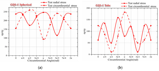
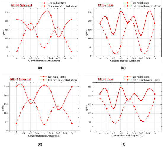
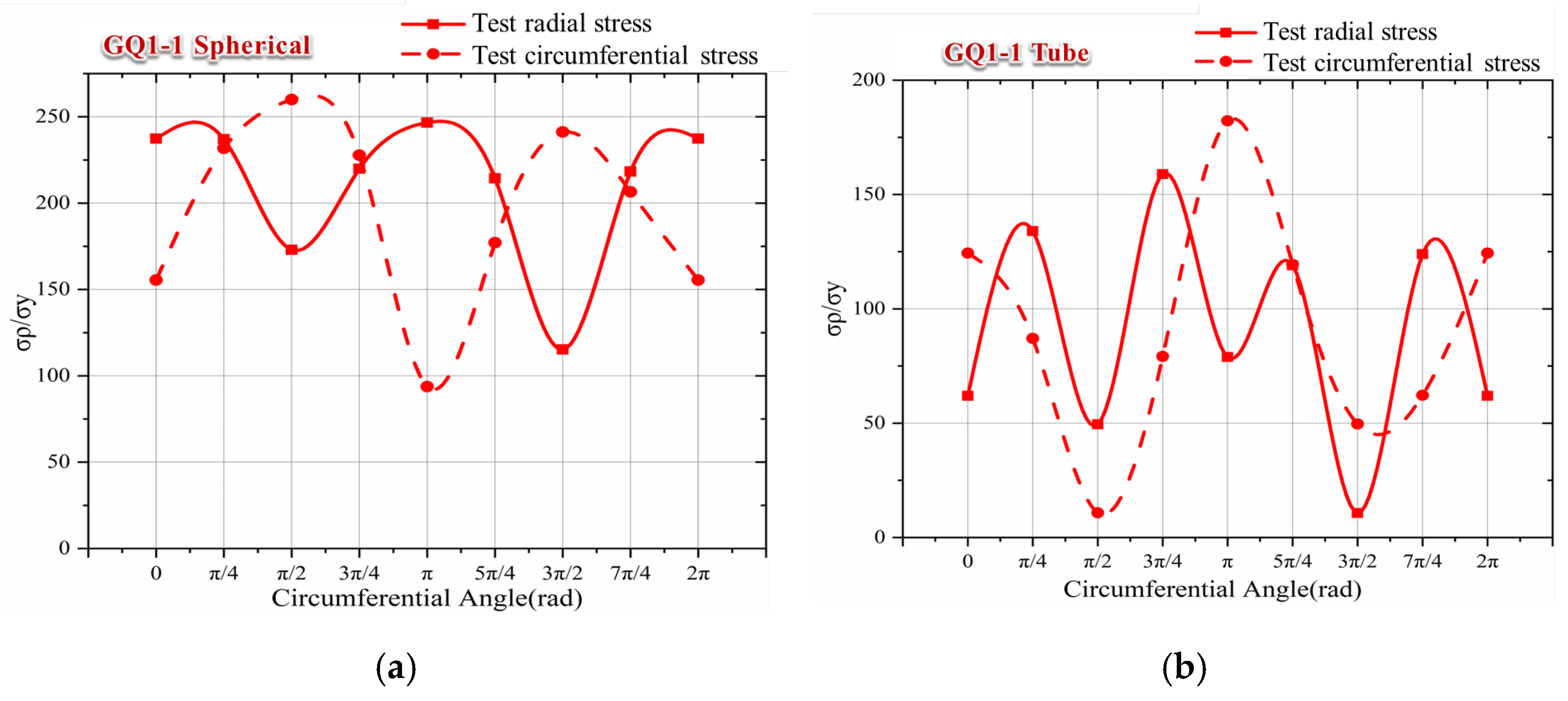
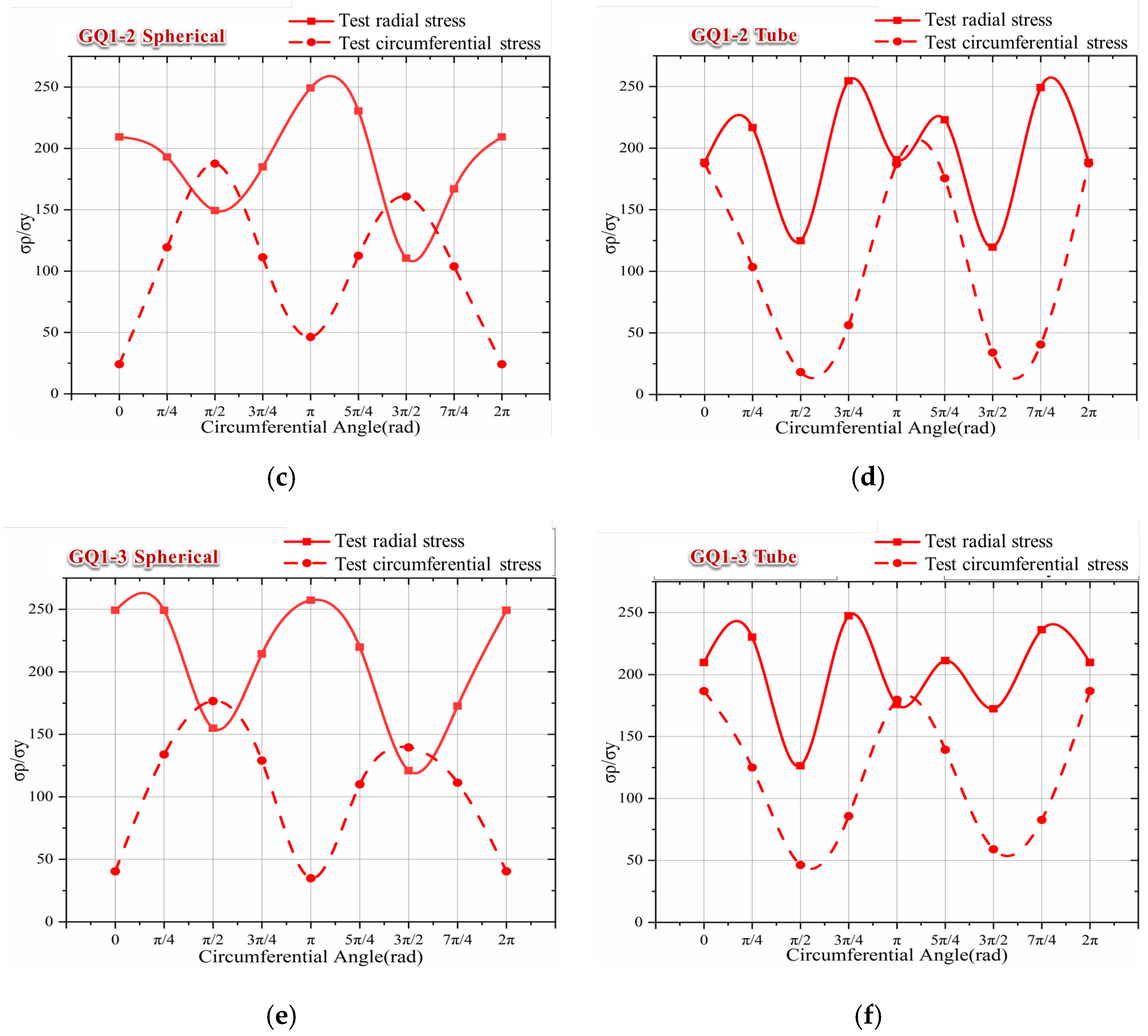
The measured strain relief is substituted into Equation (1) to compute the residual stress at the weld toe. Plasticity correction compensates for nonlinear strain response induced by stress concentration at the hole periphery. Figure 9 presents the plasticity-corrected residual stress distributions along the weld toe of the steel pipe–spherical joint for all three tested hollow sphere specimens.

Figure 9. Welding residual stress curves. (a) GQ1-1 Spherical, (b) GQ1-1 Tube, (c) GQ1-2 Spherical, (d) GQ1-2 Tube, (e) GQ1-3 Spherical, and (f) GQ1-3 Tube.

(1) Radial residual stresses at the weld toe of specimens GQ1-1, GQ1-2, and GQ1-3 range from 115 to 237 MPa, 110–249 MPa, and 120–249 MPa, respectively, and circumferential residual stresses range from 93 to 259 MPa, 24–119 MPa, and 34–176 MPa. On the spherical face (i.e., away from the weld toe), radial stresses range from 10 to 158 MPa, 119–249 MPa, and 126–236 MPa, while circumferential stresses range from 10 to 124 MPa, 18–187 MPa, and 46–186 MPa. The mean radial residual stress exceeds the mean circumferential residual stress across all specimens, whereas the standard deviation of circumferential stress is consistently higher, indicating greater spatial variability. This reflects the dominant influence of welding thermal gradients on radial stress development, which remains relatively stable in magnitude; in contrast, circumferential stress exhibits lower absolute magnitude but higher scatter, attributable to secondary effects such as local restraint variation and asymmetric cooling. (2) Both radial and circumferential residual stress distributions exhibit quasi-periodic variation along the weld toe yet lack uniform amplitude or phase—consistent with non-uniform heat input and heterogeneous cooling rates during multi-pass welding of the hollow sphere–pipe joint. These spatial irregularities underscore the need for tightly controlled welding parameters and environmental conditions in nodal hollow sphere connections. (3) Peak radial residual stress reaches 248 MPa, and peak circumferential residual stress reaches 231 MPa. Given the measured yield strength of the base material (268 MPa), these peaks correspond to 92.5% and 86.2% of σ_s, respectively. Such high magnitudes—exceeding 85% of σ_s—suggest potential interaction between adjacent blind holes: strain relaxation from a preceding hole may be perturbed by subsequent drilling, particularly when inter-hole spacing is insufficient to ensure mechanical independence. As the strain gauge readings are not acquired in real time during incremental hole-drilling, elastic–plastic strain field superposition likely occurred, introducing a systematic overestimation of localized residual stresses. This cross-hole interference constitutes a critical experimental artifact requiring mitigation in engineering practice, e.g., via increased minimum inter-hole distance (>3× hole diameter) or staggered measurement sequencing.

In this study, the hollow spherical specimen is fabricated by hot stamping two steel plates into hemispheres followed by circumferential welding—processes that may alter local microstructure and, consequently, mechanical properties. Such thermo-mechanical history can introduce discrepancies between nominal (as-received) and actual material parameters, thereby propagating uncertainty into residual stress calculations derived from elasticity-based formulations. Additionally, drilling-induced plastic deformation—including localized plastic extrusion around the hole periphery—arises from cutting forces and frictional heating; this non-elastic response further distorts strain relief measurements and inflates apparent residual stress magnitudes. To mitigate these effects in future experimental and field applications, a two-stage drilling protocol is recommended: first, pilot drilling with a 1.0 mm twist drill; second, final enlargement to 1.5 mm diameter using a dedicated blind-hole drill bit. Drilling is performed at a low, constant rotational speed (≤300 rpm) and controlled feed rate to minimize thermal accumulation and mechanical disturbance. Crucially, for curved geometries such as the hollow sphere, strict adherence to ASTM E837 requirements for hole depth (t = 0.5d ± 0.05d) and hole roundness (circularity error < 2% of diameter) is essential to ensure measurement validity. Furthermore, measurement points are positioned within 0.2 mm of the weld toe—sufficiently proximate to capture hot spot stress while avoiding direct fusion-zone interference—thereby enhancing engineering relevance and fatigue-critical applicability.

3. Finite-Element (FE) Analysis

3.1. Thermal Analysis

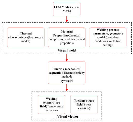
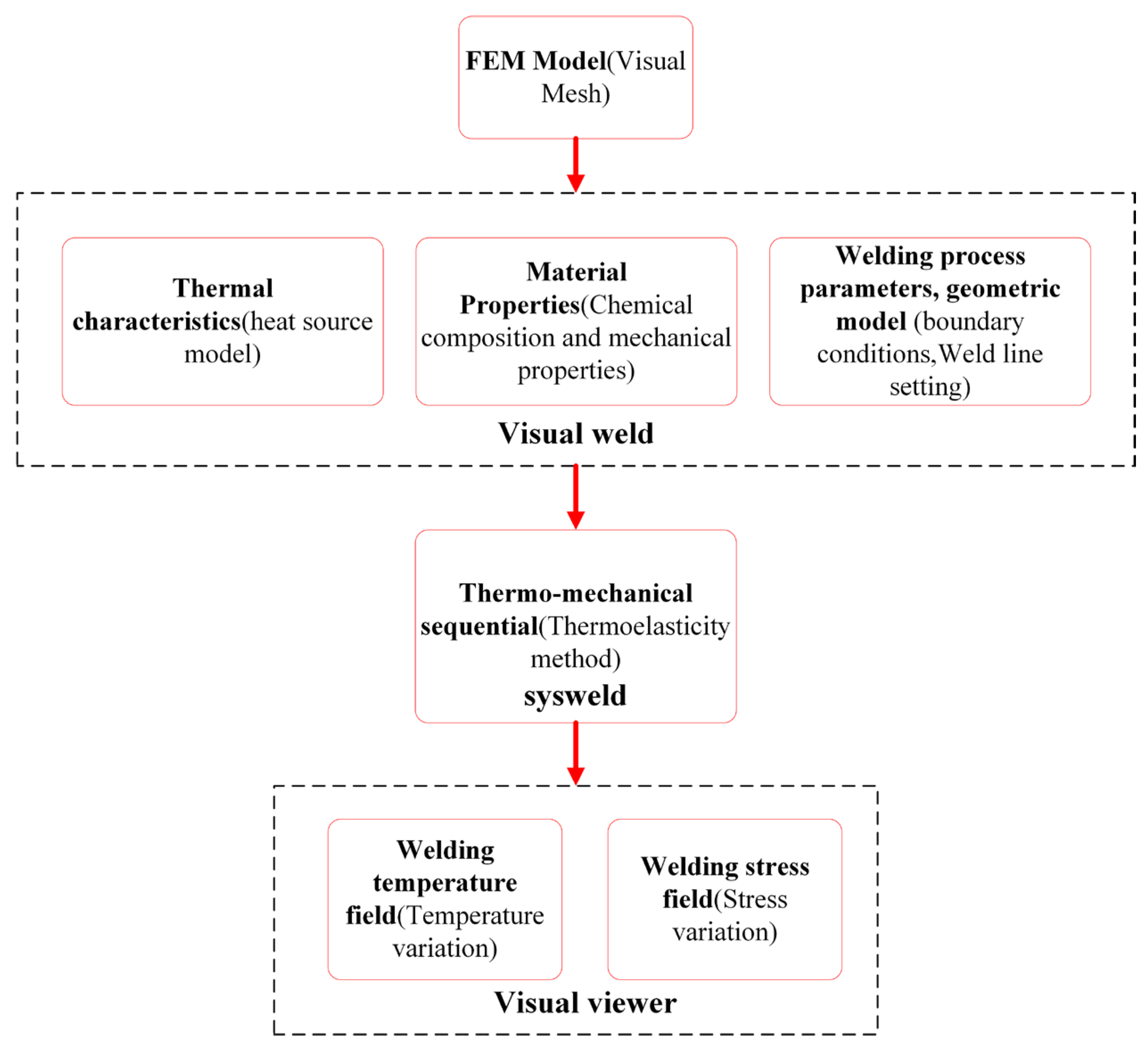
The complete finite-element analysis is grounded in both experimental data and theoretical modeling of welding residual stresses in the specimen. Visual-Mesh is employed to perform geometric modeling and mesh generation, followed by a rigorous assessment of mesh quality. Within the Visual-Weld module, the weld seam and reference line are explicitly defined, and the heat-dissipation and cooling surfaces are specified. In addition to configuring welding process parameters, the base metal and filler material are selected. Subsequently, thermoelastic simulations are conducted using SYSWELD. Post-processing of temperature and stress fields is performed via Visual-Viewer. The entire workflow is illustrated in Figure 10.

Figure 10. Numerical simulation flow chart.

3.2. Finite Element Model

The finite element model is developed using the VISUAL-Environment software (15.0), and residual welding stresses are simulated via thermo-elastic-plastic finite element analysis [27,28]. Due to the substantial heat input during the actual welding process near the weld zone, a steep temperature gradient arises in the immediate vicinity of the weld. To balance computational efficiency and modeling fidelity, a refined mesh is employed in the weld region and its adjacent heat-affected zone (HAZ), whereas a coarser mesh is adopted in the HAZ farther from the weld, where thermal gradients are milder. Mesh generation is performed using Visual-Mesh, a module within the VISUAL-Environment software (15.0) suite. The specific meshing procedure involves: (i) generating a 2D cross-sectional mesh; (ii) revolving this 2D section into a 3D solid model using the 3DRevolve function; (iii) performing a quality check on all elements using the Check function, followed by localized adjustments as needed to ensure mesh integrity. Consistent with the geometry of the welded hollow spherical joint (tube-to-ball butt weld), the weld is modeled with four passes and nine individual weld beads [29].

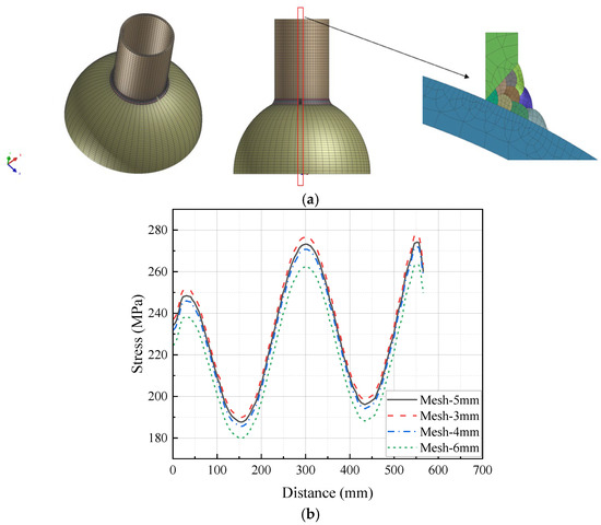
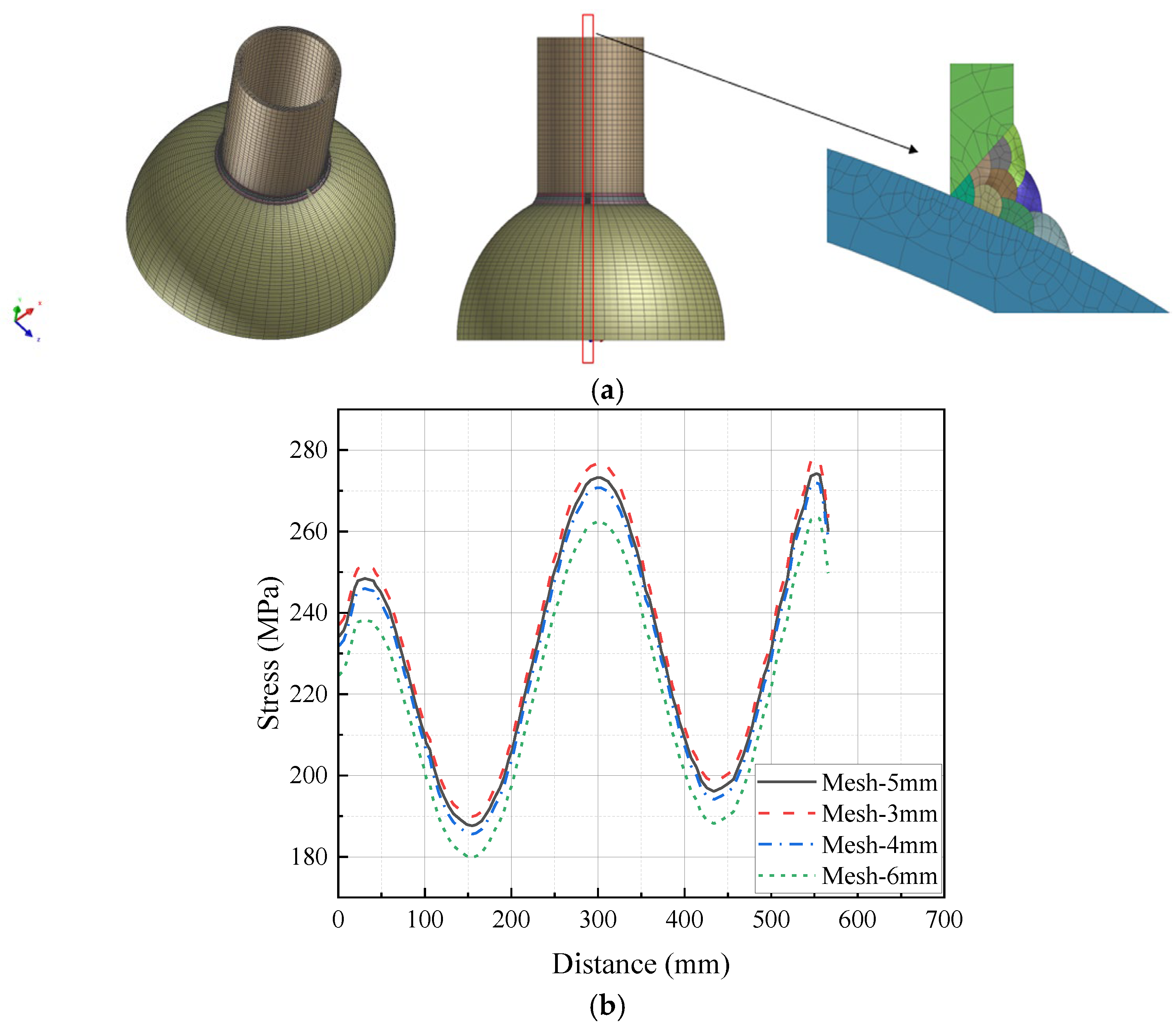
The overall model configuration and weld-specific mesh are shown in Figure 11a. Mesh convergence analysis is performed in this study to determine the minimum mesh size required for achieving convergence. Four mesh sizes (3 mm, 4 mm, 5 mm, and 6 mm) are employed. The radial residual stress at the spherical weld toe is compared across the four mesh sizes, as shown in Figure 11b. The final discretized model comprised 29,854 elements and 39,897 nodes. This mesh density strikes an optimal balance between simulation accuracy and computational efficiency. Following mesh generation, the Visual-Weld module is used to define key welding parameters, including the actual welding procedure, base material properties, weld seam geometry, weld centerline, weld reference line, weld start and end points, heat dissipation boundary conditions, and overall structural boundary conditions.

Figure 11. Finite element model and graded mesh configuration. (a) Finite element model. (b) Mesh convergence analysis.

3.3. Analysis of Welding Temperature Field

In the thermal analysis process [30], the welding temperature field is treated as a nonlinear heat transfer problem. To simplify σ_s modeling, the latent heat associated with phase change in the molten pool is neglected. The initial temperature of the workpiece is set to 20 °C (room temperature), and heat exchange between nodes and the surrounding environment is modeled solely via convection. The welding heat source is implemented using Goldak’s double ellipsoid model [31,32,33,34], which serves as the numerical heat source representation in the simulation. Within the VISUAL-Environment software, manual welding was selected as the deposition strategy, with a constant welding speed of 9 mm/s. For this configuration, the heat input is accurately represented by the double ellipsoidal heat source model [35], assessing the experimental requirements. The width and depth of each molten pool are determined experimentally through precise dimensional measurements. Notably, each subsequent weld pass is initiated only after the preceding weld had fully cooled to ambient temperature, thereby ensuring that no residual thermal influence from prior passes affected the current weld.

Setting up the base material and the welding electrode ensures that both are made of the same material. From the material library, ASTM A36 steel is selected. This grade corresponds to the Chinese standard Q235B steel. Its chemical composition is presented in Table 3, and its mechanical properties are summarized in Table 4.

Table 3. ASTM A36 chemical composition.

Trace Elements	%C	%Mn	%Si	%Cu	%S	%P
Content	0.26	1	0.4	0.2	0.05	0.04

Table 4. ASTM A36 mechanical parameters of materials.

Temperature (°C)	Modulus of Elasticity (105 MPa)	Yield Stress (MPa)	Poisson’s Ratio	Coefficient of Thermal Expansion (10−5/°C)
20	2.1	235	0.33	1.23
100	2.0	220	0.33	1.23
400	1.7	160	0.33	1.23
700	1.0	75	0.33	1.23
1000	0.5	12	0.33	1.23
1300	0.1	1	0.33	1.23
1600	0.1	1	0.33	1.23

3.4. Boundary Constraints

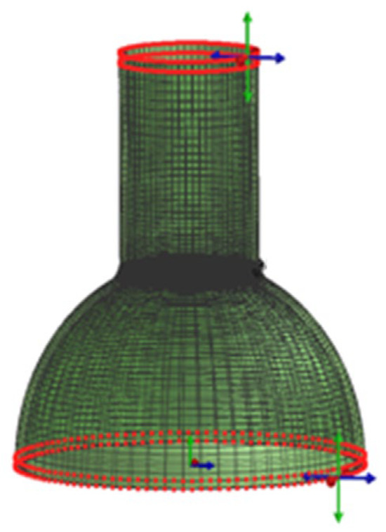
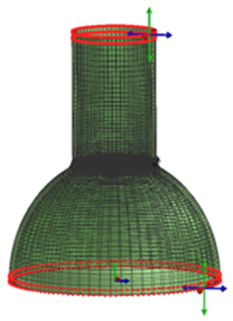
To ensure consistency between experimental testing and numerical simulation, appropriate boundary constraints are applied at the outset of the simulation to suppress rigid-body motion of the structural members. In this model, both ends are fully fixed (indicated in red in Figure 12), thereby replicating the identical boundary conditions employed during physical testing.

Figure 12. Boundary conditions of finite element model.

4. Simulation Results

4.1. Welding Temperature Field Analysis

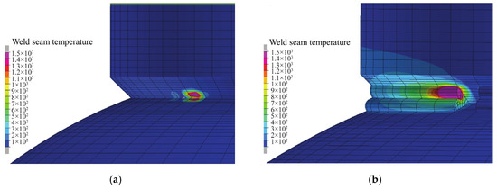
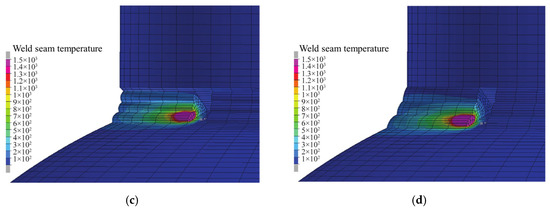
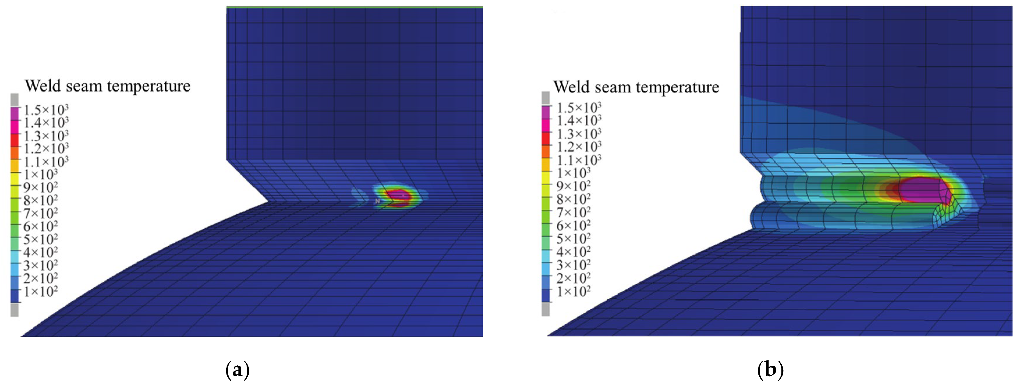
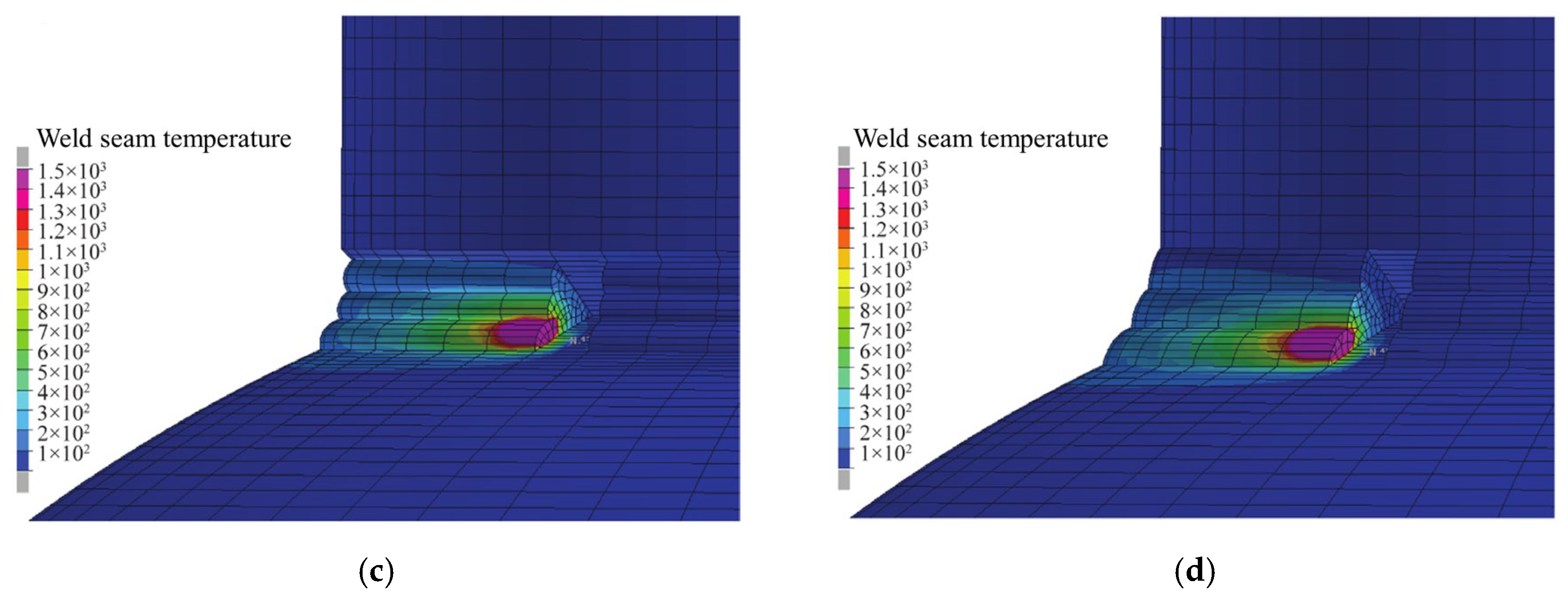
According to the welded hollow sphere node model employed during the welding process, temperature field distributions at various stages can be visualized via thermal cloud maps, revealing the molten pool geometry, the location of the peak temperature, and the location of the minimum temperature. As illustrated in Figure 13, the temperature field distribution clouds are captured at four specific instants: (i) the initiation of the first weld pass, 0.45 s; (ii) the termination of the third weld pass in the second layer, 157.65 s; (iii) the termination of the sixth weld pass in the third layer, 321.97 s; (iv) the termination of the ninth weld pass in the fourth layer, 491.89 s. Since each subsequent weld pass is initiated only after the preceding pass has sufficiently cooled, the cumulative thermal influence across passes is significantly reduced, thereby enhancing the accuracy of residual stress predictions.

Figure 13. Nephogram of the temperature field distribution. (a) 0.45 s, (b) 157.65 s, (c) 321.97 s, and (d) 491.89 s.

As shown in Figure 13, the welding heat source moves continuously over time. When the heat source approaches a given region, the local temperature rises rapidly; conversely, as the heat source recedes, the temperature of that region decreases rapidly and eventually stabilizes. During the welding process, different regions of the weld undergo sequential thermal cycles—including heating, rapid cooling, and further cooling to ambient temperature—resulting in a highly complex temperature-induced stress field.

4.2. Residual Stress Field Distribution in the Hollow Sphere–Pipe Weld Joint

Welding involves a rapid rise followed by an abrupt drop in weld temperature, resulting in highly nonlinear material behavior and significant plastic deformation, making the underlying thermo-mechanical process considerably more complex. During welding, the temperature in the vicinity of the joint typically exceeds 1500 °C. At such elevated temperatures, the steel undergoes plastic deformation. Upon completion of welding, non-uniform cooling and associated shrinkage of the plastically deformed regions are constrained by the surrounding cooler material, thereby inducing internal stresses known as welding residual stresses.

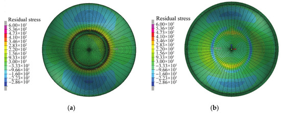
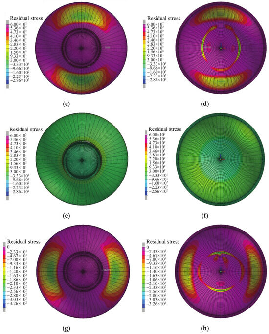
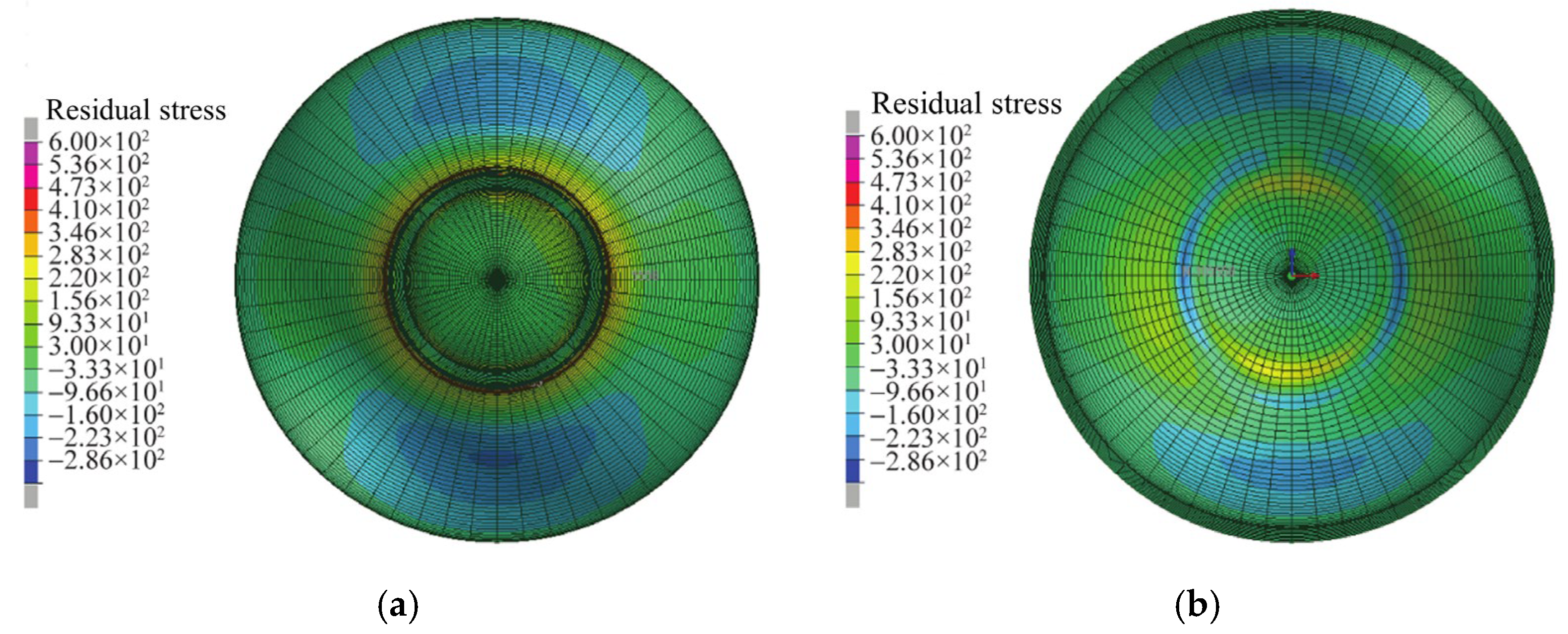
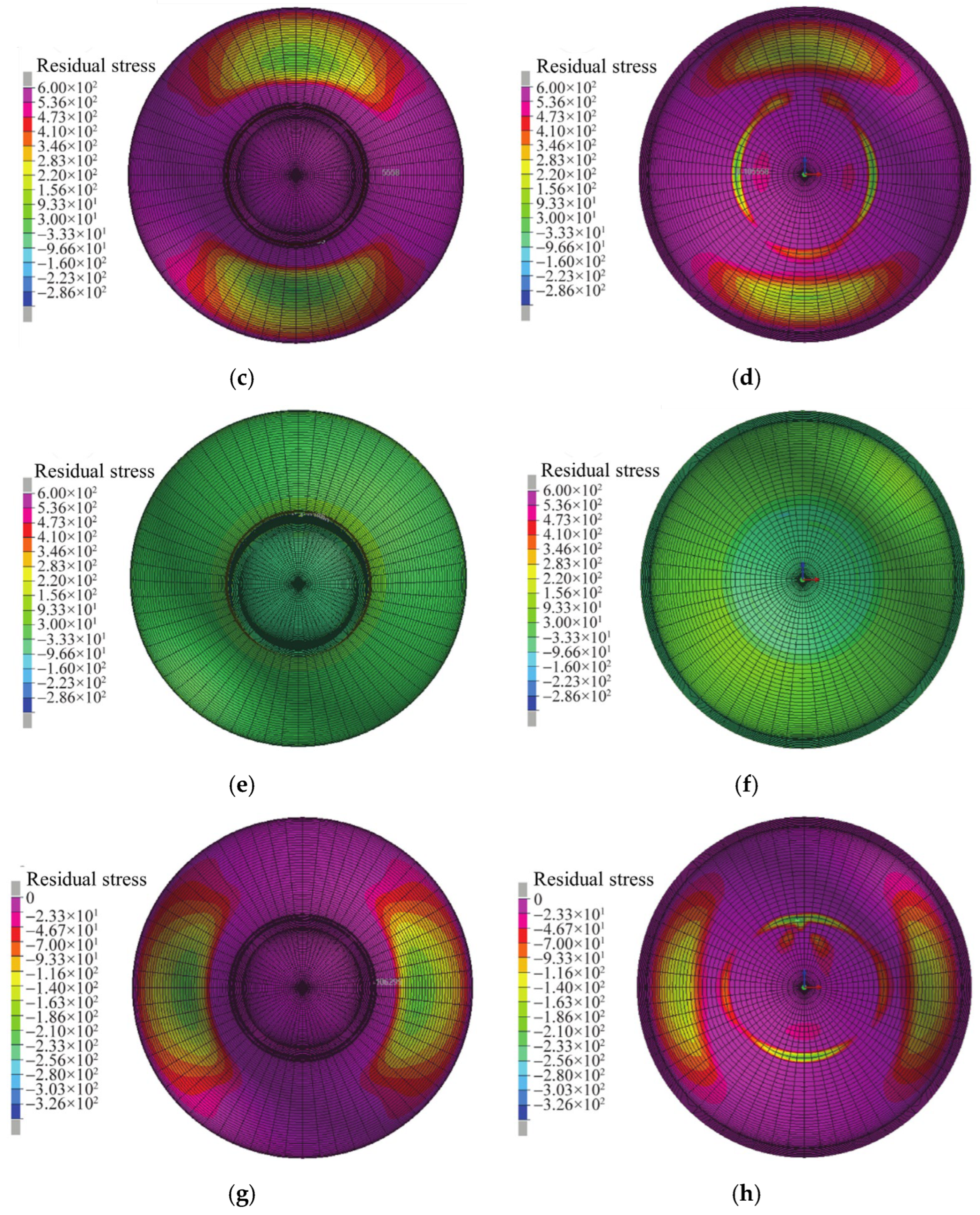
In the Visual-Weld module, the weld stress field can be computed and analyzed to investigate the distribution of residual stresses at the tube–ball weld joint of the steel tube–welded hollow spherical node. The Visual-Viewer module enables visualization of the stress distribution via a color-coded contour plot, where distinct colors correspond to specific stress intervals—see Figure 14 (residual stress distribution after welding). Notably, the tube is modeled in a cylindrical coordinate system, whereas the hollow sphere is represented in a spherical coordinate system.

Figure 14. Radial and circumferential components of residual stress at the hollow sphere–pipe weld interface. (a,b) The overall distribution of radial residual tensile and compressive stresses. (c,d) The distribution of radial residual compressive stresses on the specimen. (e,f) The overall distribution of circumferential residual tensile sub-stress. (g,h) The distribution of circumferential residual compressive stresses on the specimen.

As shown in Figure 14, both radial and circumferential residual stresses exhibit pronounced tensile dominance at the weld toes—specifically, at the toe of the spherical weld and that of the tubular weld. This tensile behavior arises from substantial heat input during welding, leading to significant residual tensile stresses at these locations. In contrast, residual compressive stresses prevail on the inner and outer surfaces of the spherical component away from the weld region, as well as at the corresponding weld toe on the inner wall of the hollow sphere. Consequently, the residual stress distribution exhibits considerable spatial variability. Overall, the residual stress field remains self-equilibrating across the entire component.

5. Comparison Between Experimental and Numerical Simulation Results

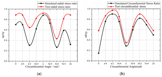
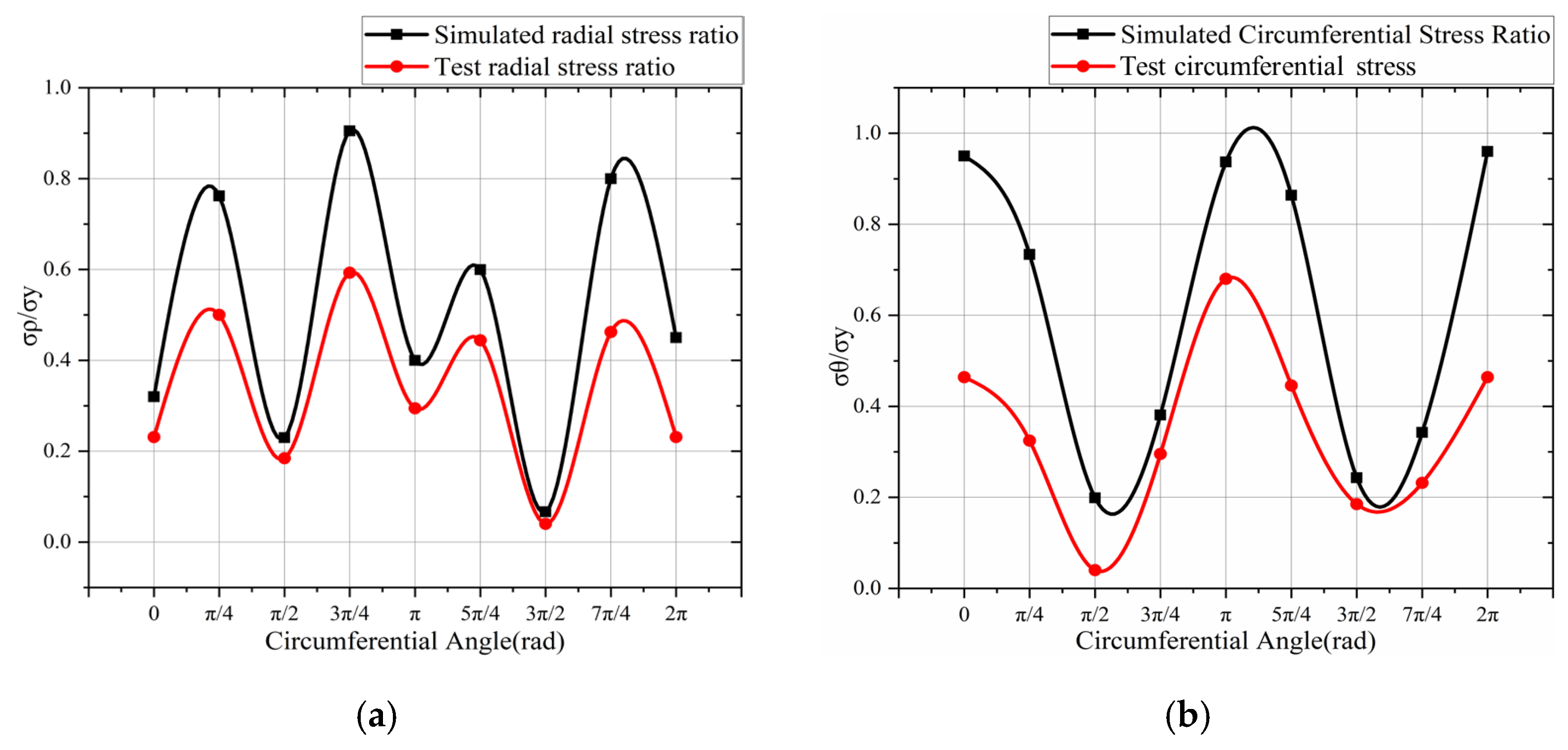
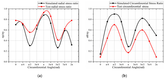
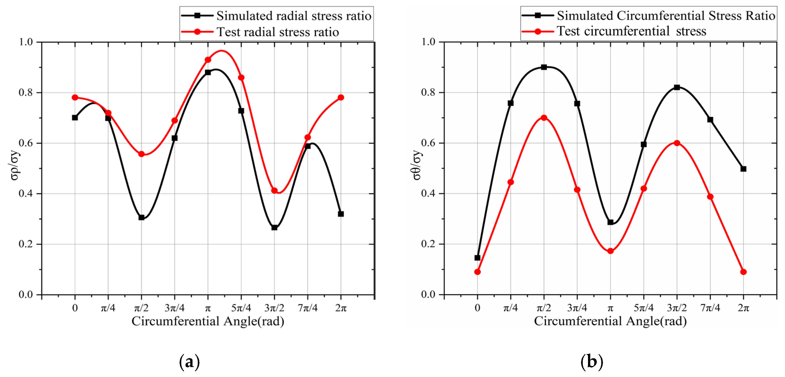
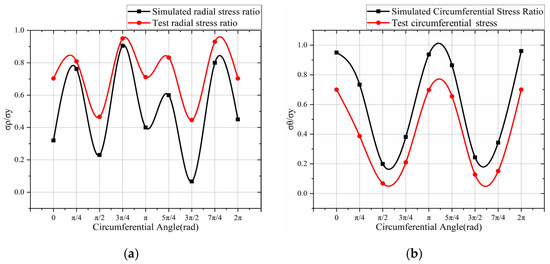
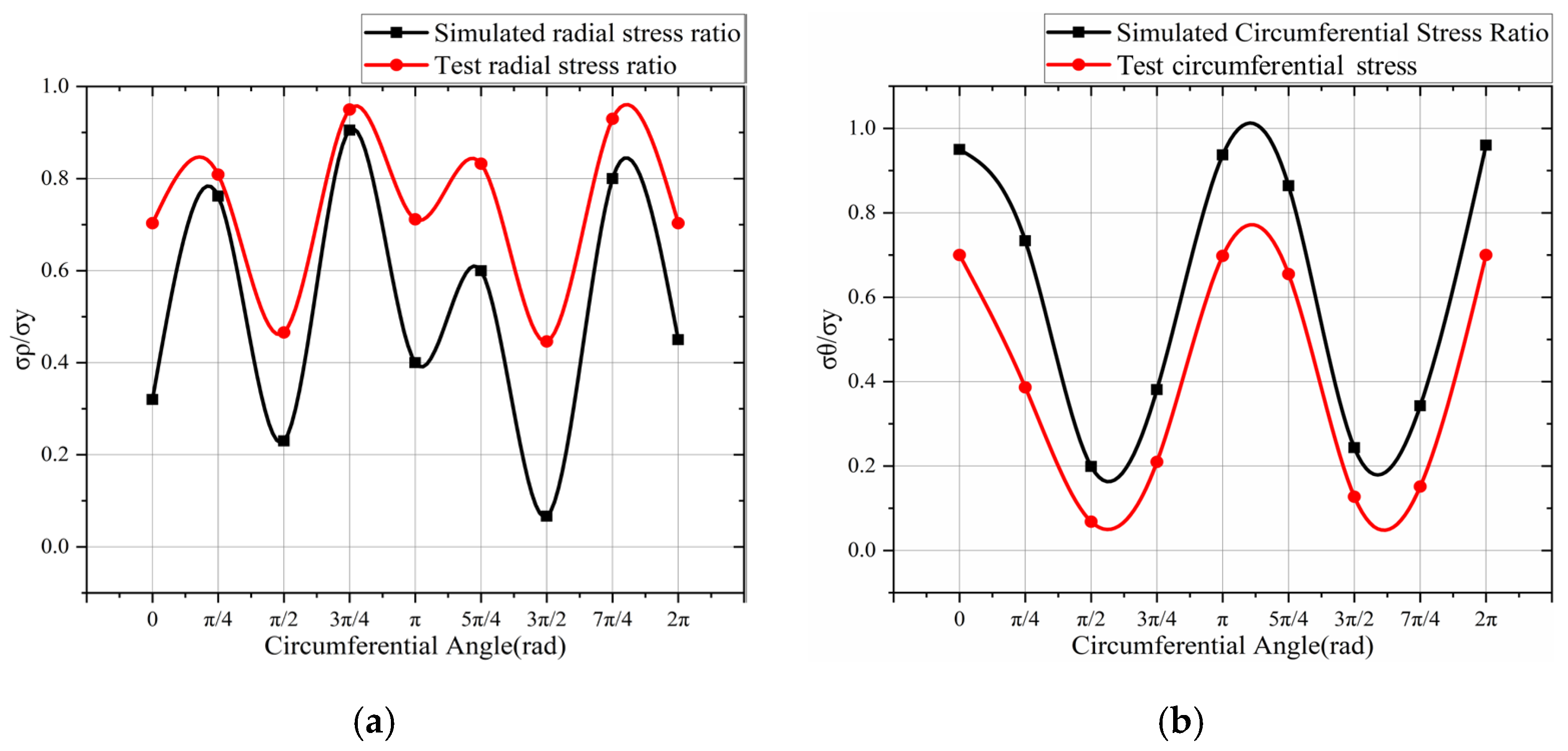
Finite element simulation results are validated against experimental measurements by aligning the simulated response paths with the corresponding test measurement locations. Specifically, identical measurement points are selected at both the spherical toe and the tube toe of the finite element model and directly compared with the experimental data; the resulting comparisons are presented as plots.

In this study, curves are plotted with the calculated yield-to-tensile strength ratio on the vertical axis and the starting arc angle on the horizontal axis. Shown below are the welding residual stress distribution curves—and their comparative analysis—for three test specimens of spherical weld toes and pipe weld toes.

(1) Specimen GQ1-1

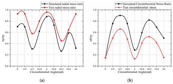
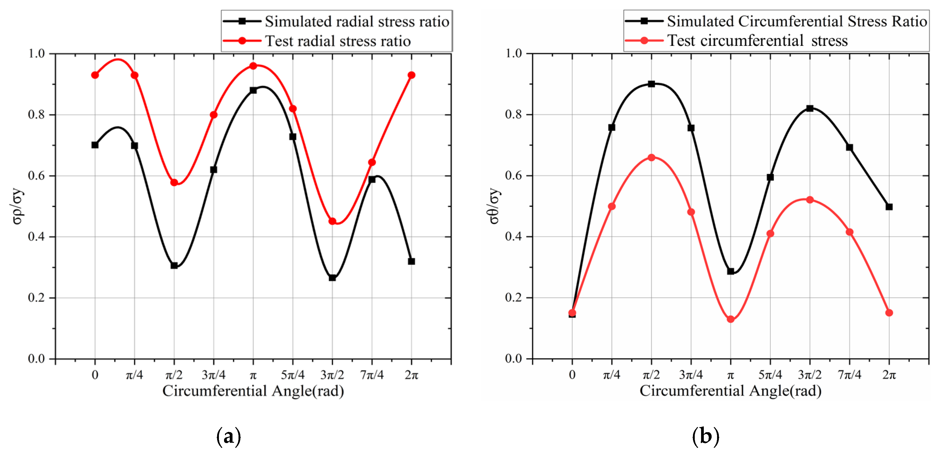
① Figure 15 presents the comparative residual stress distribution at the weld toe of the GQ1-1 hollow spherical joint.

Figure 15. Radial and circumferential residual stress distributions at the spherical weld toe: (a) radial component; (b) circumferential component.

② The comparative residual stress distributions at the weld toe of the GQ1-1 steel pipe weld are presented in Figure 16.

Figure 16. Radial and circumferential residual stress distributions at the pipe-side weld toe: (a) radial component; (b) circumferential component.

(2) Specimen GQ1-2

① The comparative residual stress distributions at the weld toe of the GQ1-2 hollow spherical joint welds are presented in Figure 17.

Figure 17. Radial and circumferential residual stress distributions at the spherical weld toe: (a) radial component; (b) circumferential component.

② A comparative plot of residual stresses at the weld toe of the GQ1-2 steel pipe is presented in Figure 18.

Figure 18. Radial and circumferential residual stress distributions at the pipe-side weld toe: (a) radial component; (b) circumferential component.

(3) Specimen GQ1-3

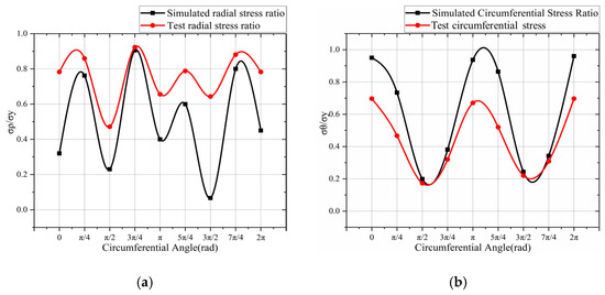
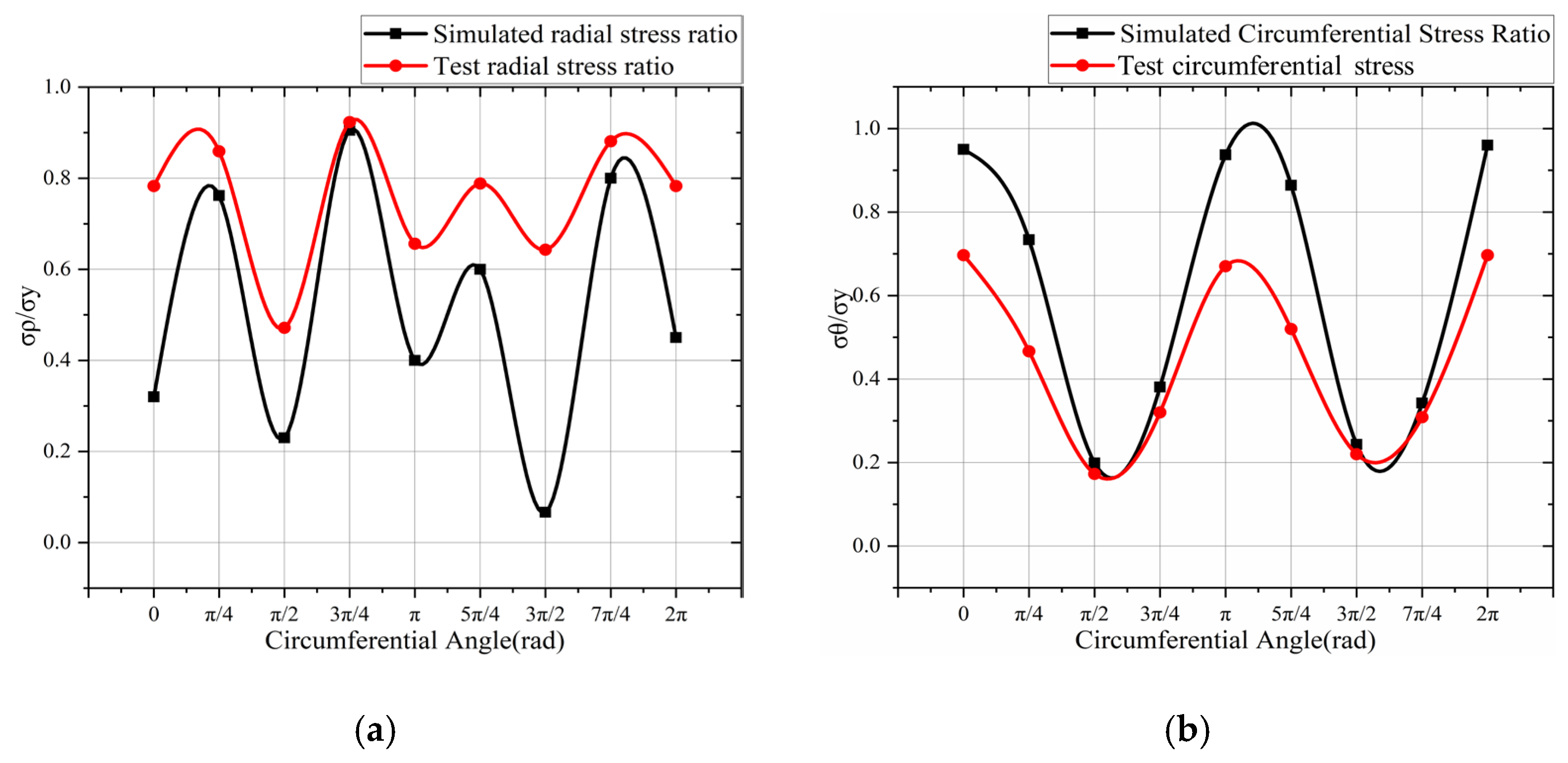
① The comparative residual stress distributions at the weld toe of the GQ1–3 hollow spherical joint welds are presented in Figure 19.

Figure 19. Radial and circumferential residual stress distributions at the spherical weld toe: (a) radial component; (b) circumferential component.

② The comparative residual stress distributions at the weld toe of the GQ1–3 steel pipe joint are shown in Figure 20.

Figure 20. Radial and circumferential residual stress distributions at the pipe-side weld toe: (a) radial component; (b) circumferential component.

Using the above comparisons, the following observations can be made:

(1)

Residual stress at the spherical weld toe: radial residual stress finite element simulation results between 0.27~0.88σ_s, with a periodic distribution and a maximum radial residual stress of 206.8 MPa; circumferential residual stress finite element simulation results between 0.146~0.9σ_s, also with a periodic distribution and a maximum circumferential residual stress of 211.5 MPa. GQ1-1, GQ1-2 and GQ1-3 spherical radial residual stress test values ranged from 0.43 to 0.98σ_s, 0.41 to 0.93σ_s, and 0.45 to 0.96σ_s, respectively, with radial residual stress maxima of 230.3 MPa, 218.55 MPa and 225.6 MPa, respectively; the annular residual stress test values range from 0.35 to 0.97σ_s, 0.09 to 0.7σ_s, and 0.09~0.7σ_s to 0.13~0.66σ_s. The maximum values of annular residual stresses are 227.95 MPa, 164.5 MPa and 154.9 MPa respectively.

(2)

Residual stresses at the weld toe of the pipe face—expressed as the ratio of calculated stress values to the steel’s yield strength (σ_s)—are investigated. Finite element simulations revealed that radial residual stresses ranged from 0.067σ_s to 0.905σ_s and exhibited a periodic distribution, with a peak value of 212.68 MPa. Annular residual stresses, likewise periodically distributed, range from 0.199σ_s to 0.96σ_s, reaching a maximum of 225.6 MPa. Experimental measurements for specimens GQ1-1, GQ1-2, and GQ1-3 yielded radial residual stresses in the ranges of 0.04σ_s–0.593σ_s, 0.446σ_s–0.95σ_s, and 0.47σ_s–0.92σ_s, respectively; their corresponding maxima are 158.9 MPa, 254.6 MPa, and 246.56 MPa. Annular residual stress measurements for the same specimens fell within 0.04σ_s–0.68σ_s, 0.068σ_s–0.699σ_s, and 0.17σ_s–0.69σ_s, respectively, with maximum values of 182.24 MPa, 187.332 MPa, and 184.92 MPa. The errors between the experimental results and simulation results are presented in Table 5.

Table 5. Error between experimental and simulated values.

Location	Mean of Experimental Values/MPa	Simulated Value/MPa	Error/%
Peak radial stress on spherical surface	224.8	206.8	8.0
Peak circumferential stress on spherical surface	182.5	211.5	15.9
Peak radial stress on pipe surface	220.0	212.7	3.3
Peak circumferential stress on pipe surface	184.8	225.6	22.1

(3)

The discrepancy between the measured and calculated residual stresses primarily arises from the following factors: ① the initial residual stresses induced during hot-pressing of the welded hollow sphere are not accounted for; ② the initial residual stresses generated during steel pipe forming are neglected; ③ the initial residual stresses generated during steel pipe forming are neglected.

6. Conclusions

In this study, weld residual stresses near the weld toe of welded hollow spherical nodes are investigated. The magnitudes of these residual stresses are experimentally determined using the blind-hole drilling method, and the associated strain-gauge stress-relief coefficient and stress–strain release curve are systematically analyzed. Concurrently, a finite-element model of the welded hollow spherical node is developed using VISUAL-Environment welding simulation software to simulate the welding thermal and residual stress fields. The numerical results are then validated against the experimental measurements. The principal conclusions drawn from this combined experimental and numerical study are as follows:

(1)

According to the temperature field analysis, the cloud map reveals that the residual stress distribution is both random and highly complex. Tensile residual stresses are concentrated at the weld toe and its immediate vicinity, whereas compressive residual stresses prevail in regions farther from the weld toe—including the inner surface of the hollow sphere. Overall, the residual welding stresses in the entire specimen are in a self-equilibrating state.

(2)

Both experimental measurements and finite element (FE) simulations indicate that, at the weld toe of the welded hollow spherical joint, the radial residual stress exhibits a periodic distribution ranging from 0.27σ_s to 0.98σ_s, while the hoop (annular) residual stress varies periodically between 0.09σ_s and 0.97σ_s. At the tube face weld toe, the radial residual stress shows a cyclic variation between 0.04σ_s and 0.95σ_s, and the circumferential residual stress varies cyclically between 0.04σ_s and 0.96σ_s.

(3)

The experimental and FE simulation results exhibit good agreement in terms of overall trend and spatial distribution pattern. However, quantitative discrepancies arise primarily due to two factors: (i) the neglect of pre-existing residual stresses in both the hollow sphere and the steel tube prior to welding, and (ii) idealized assumptions inherent in the FE modeling—such as perfect material homogeneity, geometric regularity, and simplified boundary conditions.

References

- Li, X.Z. Structure Mechanics Analysis with Different Construction Schemes in Large-Span Space Grid Structure. Adv. Mater. Res. 2013, 788, 534–537. [Google Scholar] [CrossRef]
- Han, Q.; Liu, M.; Lu, Y.; Wang, C. Progressive collapse analysis of large-span reticulated domes. Int. J. Steel Struct. 2014, 15, 261–269. [Google Scholar] [CrossRef]
- Li, Y.Q.; Tamura, Y. Nonlinear dynamic analysis for large-span single-layer reticulated shells subjected to wind loading. Wind Struct. Int. J. 2005, 8, 35–48. [Google Scholar] [CrossRef]
- Ri, N.-H.; Chen, Z.; Ri, Y.-S.; Ma, Z. Comparison of residual stress on different three-dimensional multi-layer welding methods of welded hollow sphere joint in large-span structure by considering latent heat. Int. J. Space Struct. 2019, 34, 57–73. [Google Scholar] [CrossRef]
- Jiao, J.; Lei, H.; Chen, Y.F. Numerical simulation and experimental study on constant amplitude fatigue behavior of welded cross plate-hollow sphere joints. J. Southeast Univ. (Engl. Ed.) 2018, 34, 62–70. [Google Scholar]
- Yan, Y.J.; Lei, H.G.; Yang, X. Mechanical Properties on the Welded Connection of Pipe and Hollow Spheres Joints. Adv. Mater. Res. 2011, 189–193, 3452–3457. [Google Scholar] [CrossRef]
- Liu, X. Modern Spatial Structures; Tianjin University Press: Tianjin, China, 2003. (In Chinese) [Google Scholar]
- American Welding Society. Welding Handbook, 8th ed.; American Welding Society: Miami, FL, USA, 1991; Volume 1. [Google Scholar]
- Chiumenti, M.; Cervera, M.; Salmi, A.; de Saracibar, C.A.; Dialami, N.; Matsui, K. Finite element modeling of multi-pass welding and shaped metal deposition processes. Comput. Methods Appl. Mech. Eng. 2010, 199, 2343–2359. [Google Scholar] [CrossRef]
- Akhlaghi, F. Welding Simulation and Fatigue Assessment of Tubular K-Joints in High-Strength Steel; International Atomic Energy Agency (IAEA): Vienna, Austria, 2014. [Google Scholar]
- Wang, L.; Qian, X.D.; Feng, L.Y. Effect of welding residual stresses on the fatigue life assessment of welded connections. Int. J. Fatigue 2024, 189, 108570. [Google Scholar] [CrossRef]
- Nerilli, F.; Ahmadi, H.M.; Imperatore, S.; Vairo, G. Bond–Slip Performance of GFRP Rebars in Concrete Under Alkaline and Thermal Conditioning. J. Compos. Sci. 2026, 10, 131. [Google Scholar] [CrossRef]
- Zhang, J.L.; Yan, Y.J.; Jin, S.H.; Lei, H. Fatigue tests and design of welded hollow spherical joints in grid structures. Structures 2024, 65, 106590. [Google Scholar] [CrossRef]
- Yan, Y.J.; Guo, S.C.; Zhou, Z.C. Comprehensive Fatigue Analysis and Practical Design Methodology for Weld Toes in the Sphere of Welded Hollow Spherical Joints in Grid Structures. Coatings 2024, 14, 50. [Google Scholar] [CrossRef]
- Qiu, X.B.; Huang, B.S.; Zhang, Z.; Song, H.; Qin, Y. Research on the Behavior on Axial Tensile Welded Hollow Spherical Joints Exposed to Elevated Temperature. Fire Technol. 2025, 61, 381–410. [Google Scholar] [CrossRef]
- Chen, F.H.; Zhang, H.P.; Li, Z.C.; Luo, Y.; Xiao, X.; Liu, Y. Residual stresses effects on fatigue crack growth behavior of rib-to-deck double-sided welded joints in orthotropic steel decks. Adv. Struct. Eng. 2024, 27, 35–50. [Google Scholar] [CrossRef]
- Bercelli, L.; Levieil, B.; Doudard, C.; Malek, B.; Bridier, F.; Ezanno, A. Use of infrared thermography to model the effective stress ratio effect on fatigue crack growth in welded T-joints. Eng. Fract. Mech. 2023, 292, 109061. [Google Scholar] [CrossRef]
- Vangi, D.; Tellini, S. Hole-Drilling Strain-Gauge Method: Residual Stress Measurement With Plasticity Effects. J. Eng. Mater. Technol. 2010, 132, 011003. [Google Scholar] [CrossRef]
- Ueda, Y.; Yamakawa, T. Analysis of thermal elastic–plastic stress and strain during welding by finite element method. Trans. Jpn. Weld. Soc. 1971, 2, 186–196. [Google Scholar]
- Beghini, M.; Bertini, L.; Santus, C. A procedure for evaluating high residual stresses using the blind hole drilling method, including the effect of plasticity. J. Strain Anal. Eng. Des. 2010, 45, 301–318. [Google Scholar] [CrossRef]
- Chi-Liang, K.; Ah-Der, L.; Po-Wei, H.; Hsu, C.-M. Estimation formula for residual stress from the blind-hole drilling method. Adv. Mech. Eng. 2018, 10, 168781401878740. [Google Scholar] [CrossRef]
- Wang, J.; Zhou, F. Weld residual stress measurement by small hole method. Electr. Weld. Mach. 2008, 38, 64–66. [Google Scholar]
- Zhou, F.; Wang, J.; Zhou, Y.; Zhang, J. Study on improving the accuracy of welding residual stress measurement by small hole method. Hot Work. Technol. 2007, 67–69. [Google Scholar]
- ASTM E837-20; Standard Test Method for Determining Residual Stresses by the Hole-Drilling Strain-Gage Method. ASTM International: West Conshohocken, PA, USA, 2020.
- Xu, Z.L. A Concise Course in Elasticity, 2nd ed.; Higher Education Press: Beijing, China, 1983. (In Chinese) [Google Scholar]
- Lu, S. Residual Stress Test: Small Hole Release Method; Xi’an Jiaotong University Press: Xi’an, China, 1991. [Google Scholar]
- Deng, D.; Murakawa, H. Numerical simulation of temperature field and residual stress in multi-pass welds in stainless steel pipe and comparison with experimental measurements. Comput. Mater. Sci. 2006, 37, 269–277. [Google Scholar] [CrossRef]
- Radaj, D. Heat Effects of Welding; Springer: Berlin/Heidelberg, Germany, 1992. [Google Scholar]
- Krektuleva, R.A.; Cherepanov, O.I.; Cherepanov, R.O. Numerical investigation of residual thermal stresses in welded joints of heterogeneous steels with account of technological features of multi-pass welding. Appl. Math. Model. 2017, 42, 244–256. [Google Scholar] [CrossRef]
- Choi, K.; Kim, W.; Kim, K.; Im, S.; Kim, C.-M.; Lee, J.-B. Large-scale finite element analysis of arc-welding processes. J. Phys. D Appl. Phys. 2006, 39, 2869–2875. [Google Scholar] [CrossRef]
- Azar, A.S.; Ås, S.K.; Akselsen, O.M. Determination of welding heat source parameters from actual bead shape. Comput. Mater. Sci. 2012, 54, 176–182. [Google Scholar] [CrossRef]
- Goldak, J.; Chakravarti, A.; Bibby, M. A new finite element model for welding heat sources. Metall. Trans. B 1984, 15, 299–305. [Google Scholar] [CrossRef]
- Gu, Y.; Li, Y.D.; Yong, Y.; Xu, F.L.; Su, L.F. Determination of parameters of double-ellipsoidal heat source model based on optimization method. Weld. World 2019, 63, 365–376. [Google Scholar] [CrossRef]
- Heinze, C.; Schwenk, C.; Rethmeier, M. Numerical calculation of residual stress development of multi-pass gas metal arc welding. Mater. Des. 2012, 72, 12–19. [Google Scholar] [CrossRef]
- Li, P.; Lu, H. Sensitivity analysis and prediction of double ellipsoid heat source parameters. Trans. China Weld. Inst. 2011, 32, 89–91+95. [Google Scholar]
Disclaimer/Publisher’s Note: The statements, opinions and data contained in all publications are solely those of the individual author(s) and contributor(s) and not of MDPI and/or the editor(s). MDPI and/or the editor(s) disclaim responsibility for any injury to people or property resulting from any ideas, methods, instructions or products referred to in the content. |
© 2026 by the authors. Licensee MDPI, Basel, Switzerland. This article is an open access article distributed under the terms and conditions of the Creative Commons Attribution (CC BY) license.