


Abstract
Building-Integrated Photovoltaics (BIPV) can contribute to decarbonisation, but its large-scale deployment requires accurate energy yield predictions that justify these systems during the decision-making process to ensure cost-effectiveness. In urban contexts, boundary conditions involve modelling strategies that can reliably represent the effect of shading from nearby elements. However, specific tools for proper modelling BIPV are not generally available and the workflow frequently requires the combination of different tools. Nowadays there is still no clear nor unique strategy for modelling BIPV, and expert groups are currently working on benchmarking analyses. This work compares energy yield estimations from two PV simulation software tools, System Advisor Model and PVsyst to seven years of experimental data (2017–2023) from five BIPV façade arrays distributed across three orientations (east, south and west). The main focus was twofold. Firstly, to analyse their management of shadows by following two different shading approaches: their built-in 3D modelling tools and a Digital Surface Model (DSM). Secondly, to evaluate the capability of these tools to simulate the performance of real BIPV systems. Results manifest that conventional and accessible PV software can be suitable for BIPV modelling as long as care is taken to properly assess the effect of shading, especially from urban tree canopies. The novel DSM strategy proposed is proven effective and can be a valid alternative in certain cases when the availability of in situ data is limited.
1. Introduction
Improving energy performance in buildings is essential for the goal of achieving zero-emission and fully decarbonised cities [1]. Meanwhile, energy efficiency in buildings is drawing the interest of decision-makers globally. For instance, recent directives from the European Union aim to reduce energy consumption by more than 10% by 2030 [2] and promote the use of renewables in buildings [3]. Photovoltaic (PV) systems are widely used to convert building surfaces into energy generators to contribute to achieving net-zero energy buildings. Rooftop PV represents the most widespread application of PV in buildings, typically as Building-Attached Photovoltaics (BAPV). Alternatively, PV modules can be seamlessly incorporated into building envelopes as Building-Integrated Photovoltaics (BIPV) [4,5], serving as both constructive elements and energy generators with enhanced aesthetic, thermal and structural performance [6]. However, BIPV deployment is still limited due to integration challenges, lack of standardisation, and concerns regarding cost-effectiveness [7]. In this context, reliable modelling of BIPV systems performance is crucial to promote and extend its deployment.
Modelling the performance of BIPV systems is more challenging than modelling that of conventional PV. Orientation, tilt and other boundary conditions for BIPV highlight the particularities involved in simulating PV conversion in façades, complex rooftops and other building elements. Partial shading and non-optimal azimuthal deviations are common in many BIPV applications. In addition, the variety of building elements where PV can be integrated is extensive (rooftops, façades, tiled roofs, skylights, canopies, windows, balconies), which adds complexity to the modelling workflow [8,9,10,11]. Therefore, it is common to use more than a single simulation tool when modelling BIPV systems [12]. Yang et al. reviewed different solar PV simulation tools, remarking their strengths and drawbacks for BIPV applications [13]. Moreover, a group of experts under Task 15 of IEA-PVPS presented an exercise of modelling a BIPV case study with different tools; they pointed out the limitation of standalone PV tools for 3D modelling characterisation as well as the limited electrical capabilities of other 3D software [14].
Accurate characterisation of the incoming solar irradiance (plane-of-array, POA) is the first essential step in modelling any PV system. In the particular case of BIPV, the determination of a reliable 3D topology plays a crucial role for properly evaluating shadow casting. Solar cadastres and solar potential studies have proposed different methods for constructing urban 3D scenes. The use of a Digital Surface Model (DSM) generated from Light Detection and Ranging (LiDAR) imagery using Geographic Information Systems (GIS) is widely found in many methodologies [15,16]. For BIPV façade applications, the accuracy of the DSM notably influences the correct estimation of POA irradiance and shadows on every element of the façade [17,18,19]. Thus, the initial step in modelling the energy performance of BIPV systems consists of creating a 3D building model and exporting it to the subsequent PV performance model.
Recent years have witnessed a growing interest in automating and integrating the various stages of the BIPV design workflow. For instance, autonomous frameworks combining Unmanned Aerial Vehicle based 3D survey, deep-learning point-cloud reconstruction and life-cycle cost assessment have been proposed to support BIPV deployment decisions [20]. Purpose-built BIPV simulators integrating 3D panel layout generation with techno-economic assessment have been developed for industrial buildings [21], and integrated design methodologies combining shadow calculation, irradiance-based resource assessment and automatic module arrangement have been proposed as alternatives to the sequential use of separate tools [22]. Current developments are encouraging, yet validation has tended to focus on idealised conditions or rooftop applications, and transferability to complex urban façade environments—where azimuth and shading conditions are relevant—remains largely unexplored.
In parallel to shadow casting, input data for the solar resource highly influences final energy prediction. Conventional PV modelling tools apply a transposition model to estimate POA irradiance from the solar radiation components (direct normal, DNI, and diffuse horizontal, DHI). High quality datasets with these solar components are available from satellite-derived solar irradiance models for almost every geographic coordinate worldwide. The Photovoltaic Geographical Information System (PVGIS) [23,24,25], the Copernicus Atmosphere Monitoring Service (CAMS) radiation service [26,27,28] and the National Solar Radiation Data Base (NSRDB) [29] are some of the most popular solar radiation products available. In addition, several studies have recently evaluated the accuracy of these solar services [30,31,32]. Common PV performance models are able to use hourly or sub-hourly time series of meteorological input data including the solar radiation components and other influencing variables such as temperature or wind speed and direction.
Several gaps remain unaddressed regarding BIPV façade performance modelling. Evidence on how shading characterisation strategies affect energy yield predictions in widely used simulation tools is still scarce, and practical implications of using LiDAR-derived 3D scenes instead of simplified near shading objects have not been evaluated for façade applications. The present work aims to quantify the effect of shading characterisation strategy and 3D scene choice on energy yield predictions for five real BIPV façade arrays in an urban environment under Mediterranean climate (Madrid, Spain). This study is conducted over a seven-year period (2017–2023) on an hourly basis using two well-known conventional PV tools: System Advisor Model (SAM) [33] and PVsyst [34], providing uncertainty bounds that can guide practitioners in balancing modelling effort against predictive accuracy. Both simulation tools can be considered standards in modelling PV system performance nowadays. This paper evaluates their performance when characterising the effect of shading following two different strategies: (a) by importing a 3D model from a previously created DSM derived from LiDAR imagery, and (b) by using the 3D scene created with the near shading tool included in each software. The results, regardless of the PV tool used for computing the energy performance, highlight the importance of proper characterisation of the surrounding topology for a BIPV façade system. Despite SAM and PVsyst being tools originally designed for conventional PV systems, their universality, availability and widespread use make them attractive for analysing and simulating many different PV applications, such as BIPV systems. Therefore, the uncertainty analysis of this kind of PV modelling tools when applied to BIPV solutions may help significantly to the design and decision-making processes in BIPV deployment for both new and retrofitting projects. Moreover, the analysis of different options for dealing and characterising shading on a BIPV façade might be quite relevant in terms of quantifying the effort and accuracy needed for reliable energy yield estimations.
Following this introduction (i.e., Section 1), the remainder of the document is structured as follows: Section 2 (Materials and Methods) outlines the performed simulation analysis by describing the BIPV monitored case study, the main assumptions of SAM and PVsyst models, the two strategies applied for shading losses (3D scene versus DSM), and the meteorological data used in calculations; Section 3 presents the results obtained from evaluating both simulation tools against experimental data; key findings and takeaways are discussed in Section 4; and lastly Section 5 summarises the relevance of the presented work in its context, encouraging further research in the field.
2. Materials and Methods
This paper evaluates the performance of two PV simulation tools (SAM, version 2025.4.16, and PVsyst, version 8.0.15) in energy yield estimation applied to a BIPV case study, with special attention to the definition of shading losses (mainly due to surrounding tree vegetation) following two modelling strategies: (a) the built-in 3D tool provided by each software, and (b) a DSM that represents the 3D topology. The case study involves an existing building with five BIPV arrays distributed across three façades (east, south and west) monitored since 2017. Simulation results, obtained hourly, are compared to in situ experimental values based on seven years of data (2017–2023).
The experimental database is lengthy enough to assess the performance of the different BIPV arrays while accounting for the inter-annual variability. This is not common in many BIPV modelling exercises, which are usually limited to one single year of experimental data. Therefore, the multiyear modelling and assessment avoids potential biases that may result from using one year of modelling due to the expected fluctuations of solar radiation over time.
2.1. Technical and Graphical Description of the Case Study and Urban Context
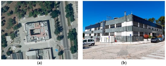
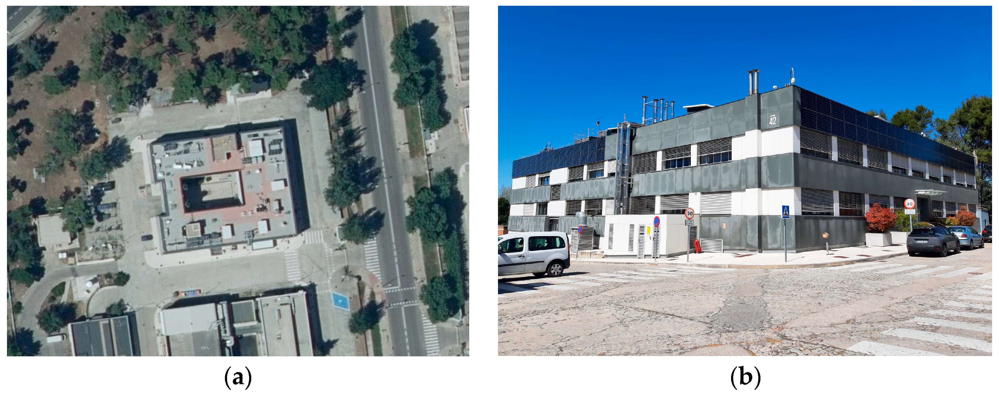
The building under study, hereafter referred to as Building 42, is located at the CIEMAT campus in Madrid (40.45° N, −3.74° E), Spain. BIPV arrays were integrated into the top areas of the east, south and west façades as part of the building’s renovation in 2017. The building is nearly aligned with the cardinal directions, with a 7.35° azimuth offset toward the southeast (Figure 1).
Figure 1.
Building 42 at CIEMAT campus: (a) aerial view (Source: PNOA 2023 CC-BY 4.0 scne.es); (b) street-level view of the southeast corner.
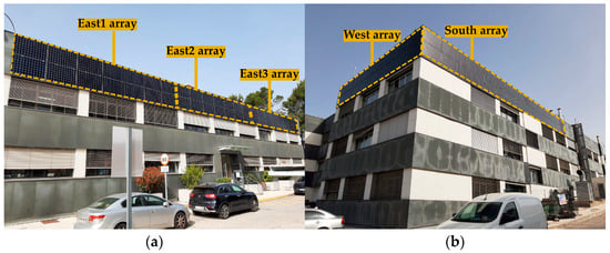
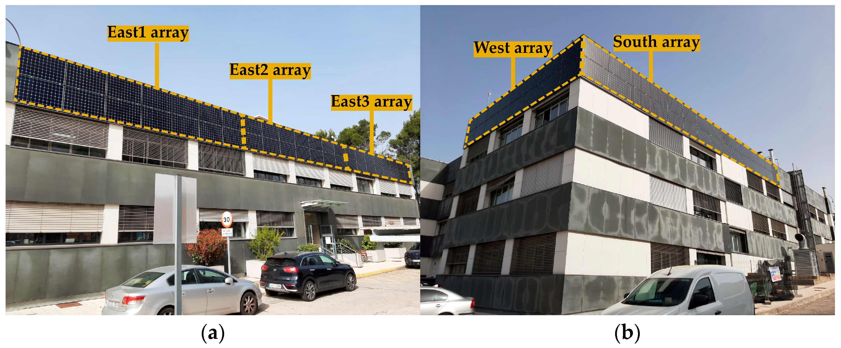
The renovation of Building 42 involved the construction of a ventilated façade where BIPV arrays were integrated. The façade incorporates a seven-centimetre air gap cavity with a 1.5-centimetre top opening, enabling some degree of ventilation on the modules’ rear-side. Figure 2 highlights the layout of the five analysed BIPV arrays across the three façades: the east façade is divided into three separate arrays with 14 modules each (7sx2p), the south array comprises 28 modules (7sx4p), and the west façade includes 16 modules (8sx2p).
Figure 2.
Building 42 in CIEMAT campus: (a) arrays on the east façade; (b) arrays on the west and south façades.
The main technical characteristics of the five BIPV arrays are summarised in Table 1. Specifications for the modules used on the south array (E18-305) show an efficiency of 18.7% and a nominal power of 305 W, while those on the east and west arrays (E20-3027) reach values of 20.1% and 327 W. Each array is connected to an independent inverter, the south array having the highest nominal power output at 8 kW, while 4 kW inverters are used for the east and west arrays.
Table 1.
Technical characteristics of the BIPV systems in Building 42.
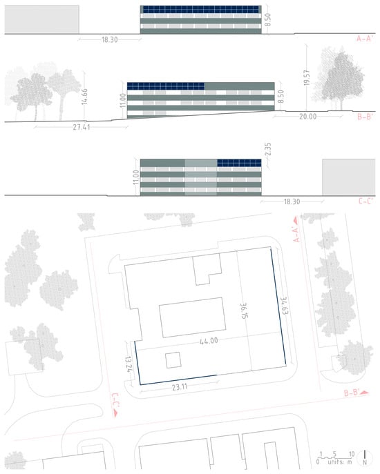
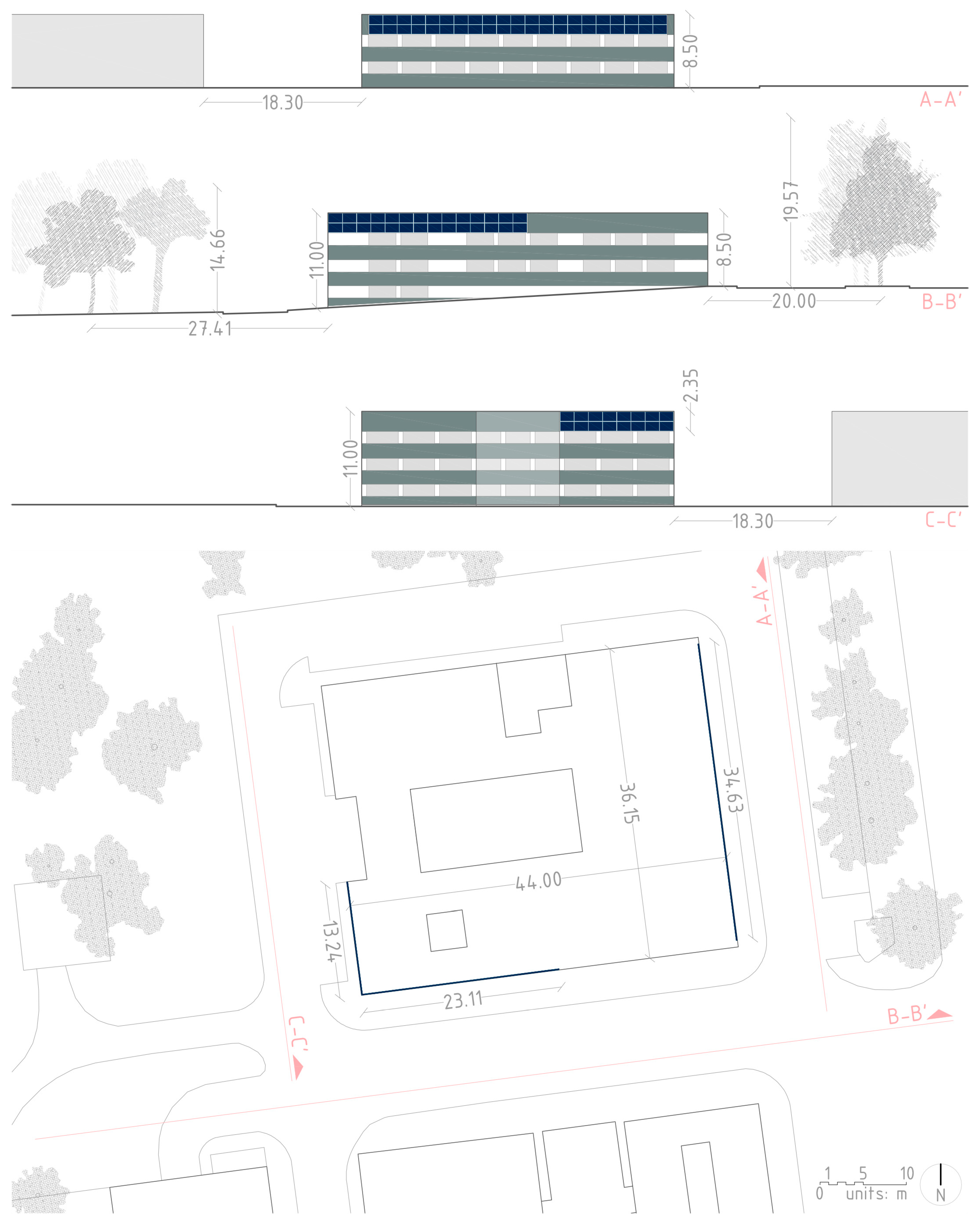
For a technical graphic representation, Figure 3 presents the building’s elevations and site plan, including nearby elements (surrounding vegetation and neighbouring buildings), as well as annotations of the most relevant dimensions and relative distances. Site plan information was derived from the Spanish Cadastral Institution, and building and tree heights were estimated from in situ measurements and data collection. The three elevations show the placement of the PV arrays on the upper areas of the east (section A-A’), south (section B-B’) and west (section C-C’) façades. Tree shapes and sizes are based on in situ information in an attempt to be representative of the actual urban conditions.
Figure 3.
Building 42: elevations (east: A-A’, south: B-B’ and west: C-C’) and site plan. Scale: 1:600. PV modules are represented in blue. (Source: Work derived from the Cadastral Electronic Site from the Spanish Cadastral Institution).
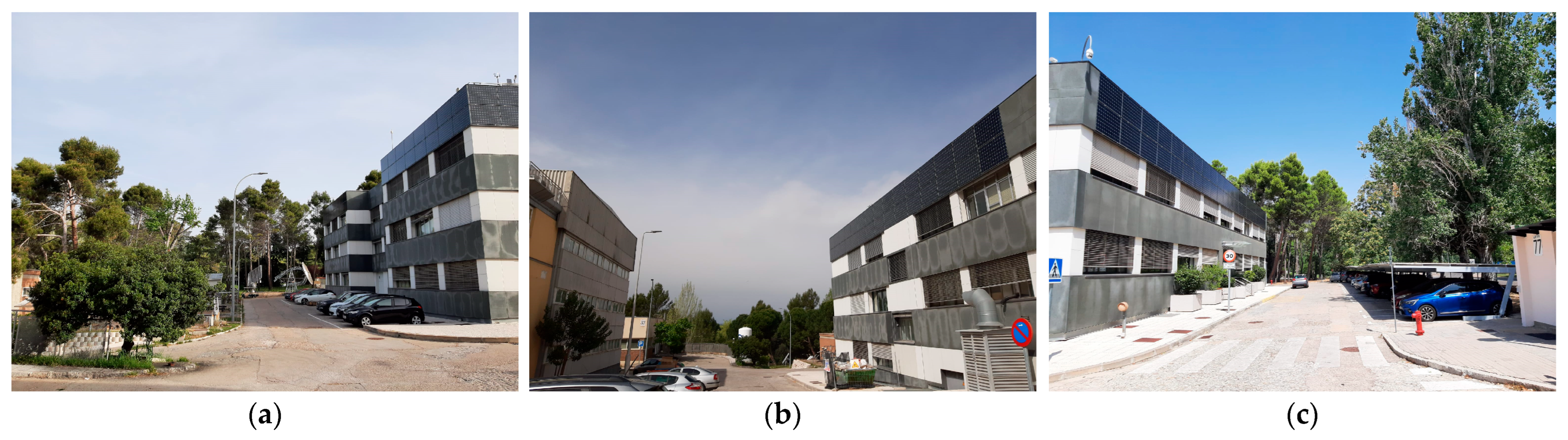
The shading context is further reflected in Figure 4 with images of the surroundings for the west, south and east façades, respectively. The impact of trees on the east array is noticeable given their relative height and distance in relation to Building 42, whereas those affecting the west array have minimal impact. Additionally, the effect of the neighbouring building on the south façade was found to be negligible.
Figure 4.
(a) Vegetation near the west array; (b) building near the south array; (c) vegetation near the east array.
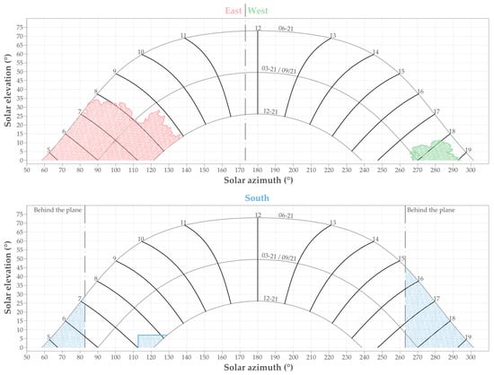
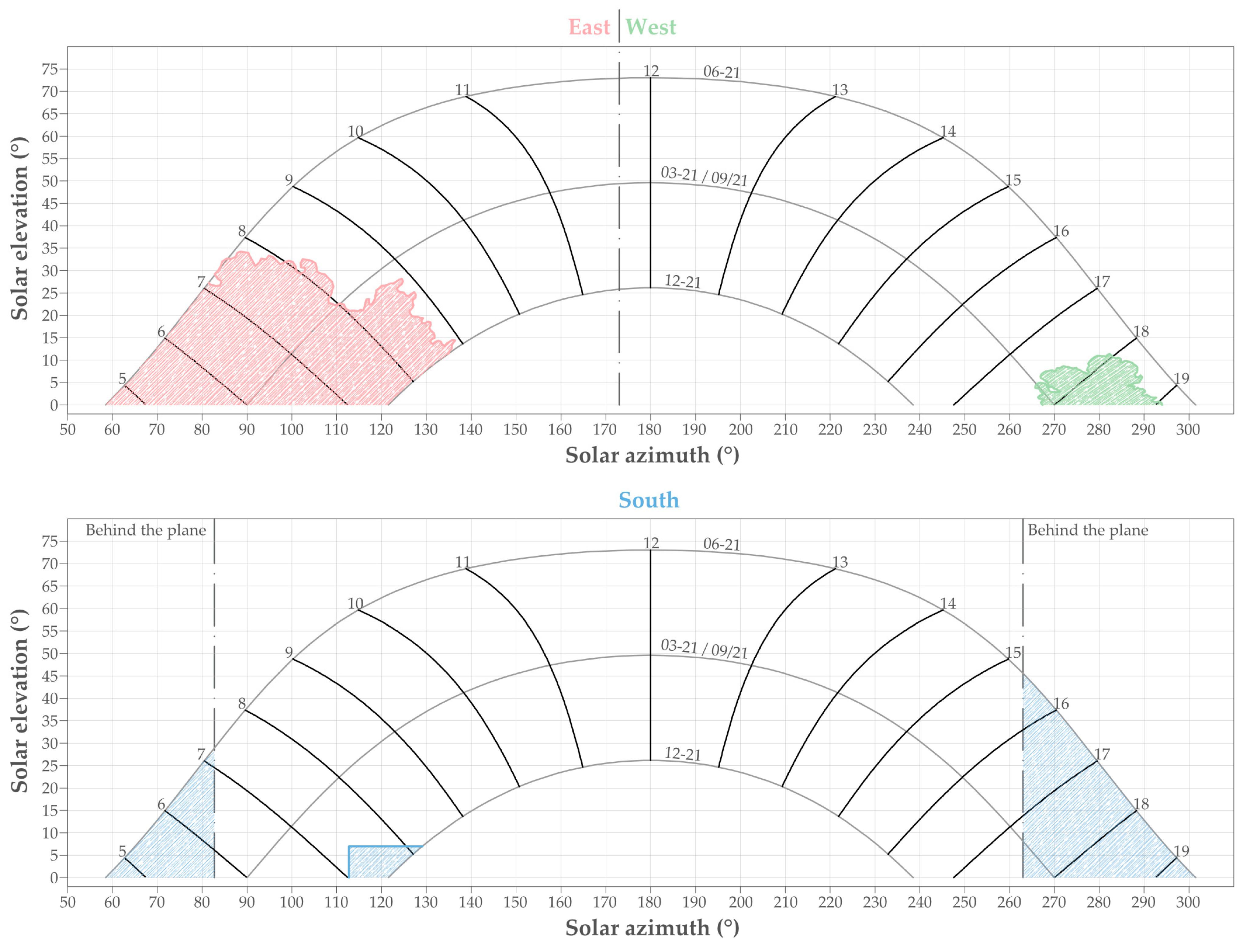
Finally, for a schematic analysis of shading, Figure 5 presents sun path diagrams based on solar azimuth and elevation angles, with the base point set at the bottom-centre of the array in each façade, to show the visibility of obstacles or lack thereof. Given that the field of view of the east and west façades are complementary, their diagrams are combined into one, where the dashed line indicates when the sun is behind the plane in each orientation, respectively. The two outer lines represent the summer (21 June) and winter (21 December) solstices, and the middle one the spring and summer equinoxes (21 March and 21 September), while the tilted lines reflect the hours throughout the day from 5 am until 7 pm. The east and west sun path diagram shows the surrounding tree canopies, and when these generate shading for each array. The south array is only affected by the corner of the neighbouring building for a small fraction of time.
Figure 5.
Sun path diagram and obstacles for east (pink), west (green) and south (blue) BIPV façades.
2.2. Development of Simulation Models in SAM and PVsyst: 3D Scene and DSM
As mentioned earlier, two simulations were performed for each PV tool: (a) using the built-in 3D modelling tool, and (b) through a DSM. The main parameters for project site location, including latitude, longitude, altitude and time zone, are contained in the weather file in SAM and set in a dedicated menu in PVsyst.
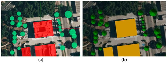
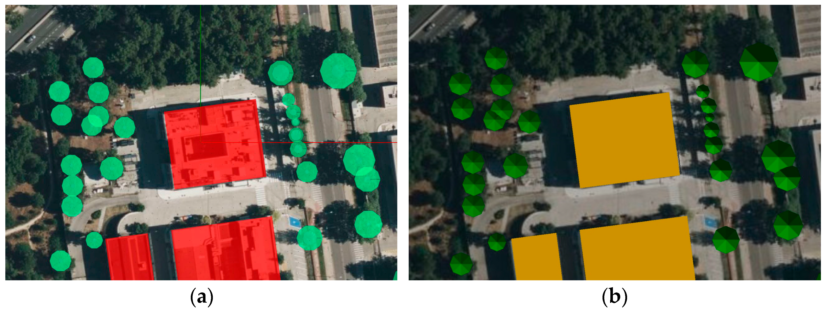
The first strategy was to create a 3D scene with the built-in tool of each simulation program, which implies manually drawing the objects on flat ground surface and adding each element individually (Figure 6). Dimensions and relative distances are estimated from the building’s architectural drawings, in situ measurements and observations, supported by a scaled satellite image as background. PVsyst provides a 3D tool with higher operability, more customisable tree definition, and a user-friendly interface similar to other architecture-oriented software. SAM, on the other hand, offers a simpler tool that covers basic design requirements and parameters.
Figure 6.
3D models developed using the built-in tools: (a) SAM 3D shading scene tool; (b) PVsyst near shading tool. Buildings are represented in red (SAM) and yellow (PVsyst), trees are shown in green tones.
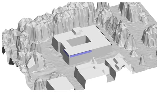
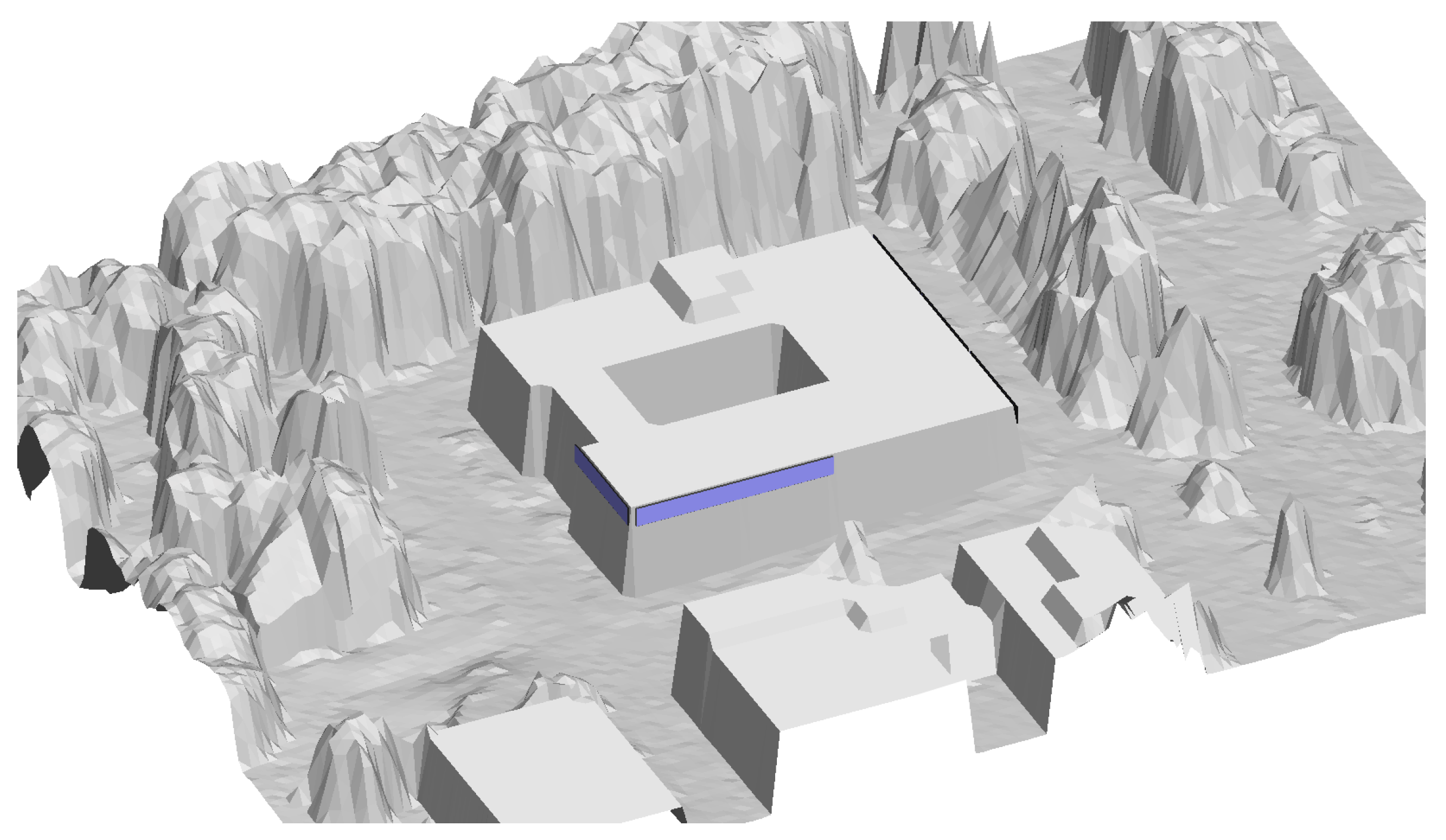
For the second approach, a DSM was created from LiDAR using GIS tools (QGIS version 3.40.15 and LAStools version 2.3.2). This procedure relies on databases, usually online, rather than in situ measurements, providing a more automated process that can reduce computational time. In previous research, the authors proposed a methodology that combines vector building footprints, obtained from building cadastres, with a LiDAR point cloud to develop a high-resolution DSM with buildings and vegetation [35]. That methodology has been applied in the present work to create a DSM that represents the local 3D topology. LiDAR input data, obtained from the Spanish National Geographic Institute (IGN), corresponds to flights conducted in August and September 2016 with a density of 1 point per square metre. Following a spatial resolution of one pixel per LiDAR cloud point, the DSM was created with a grid of 1 metre per pixel both horizontally and vertically. This DSM was imported into the near shadings menu in PVsyst, and PV modules were then placed manually (Figure 7).
Figure 7.
Rendering of the DSM in PVsyst. PV modules are represented in blue. (Work derived from LiDAR-PNOA-cob2 2016 CC-BY 4.0 scne.es and CartoBase ANE 2006–2024 CC-BY 4.0 ign.es).
2.3. Definition of Vegetation and Limitations
Whether using the 3D scene or the DSM strategy, a key challenge is properly defining the vegetation surrounding the BIPV systems for accurate simulations. Overall, the 3D scene allows more customizability when designing individual trees but can be time consuming if the number increases significantly, in addition to needing in situ information. The DSM, on the other hand, can handle larger areas with dense vegetation more easily, yet it is subject to data availability. Furthermore, there are several aspects where both workflows require special consideration, as outlined hereunder.
An important aspect when dealing with vegetation is accounting for seasonal variability in canopy foliage within the simulations—particularly for deciduous trees—rather than using the same tree definition throughout the entire year. However, neither of the analysed tools currently allows the vegetation to change over time within a single simulation. Instead, different shading setups must be defined with varying tree properties, and calculations must be performed separately for each setup. To include these seasonal changes, trees could be modelled with full foliage from April to September and with partial foliage from October to March. Although this approach is feasible and can improve accuracy, it leads to a complex and time-consuming workflow that requires combining output data from multiple simulations. Furthermore, some parameters—such as the performance ratio—must be calculated for the entire year and therefore cannot be directly combined or averaged from separate simulations, requiring additional user intervention.
Another limitation of the analysed workflows is defining partially foliated trees in the simulations, given that tree elements are represented as solid objects in the evaluated tools. A possible approach is to redefine tree canopies with a smaller diameter, although this is not a realistic representation. To address this issue, Lindberg et al. developed a QGIS plug-in, the Urban Multi-scale Environmental Predictor [36], which isolated vegetation as a separate layer and assessed seasonal variations by estimating light transmissivity through the tree crown according to tree species [37]. However, this methodology is only applicable within the QGIS software and would require PV simulation software to process two different layers (i.e., base elements + vegetation), which is not currently possible. As a suggestion, this light transmissivity concept could be added to the 3D scene tools of SAM and PVsyst as a customizable parameter in future updates.
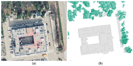
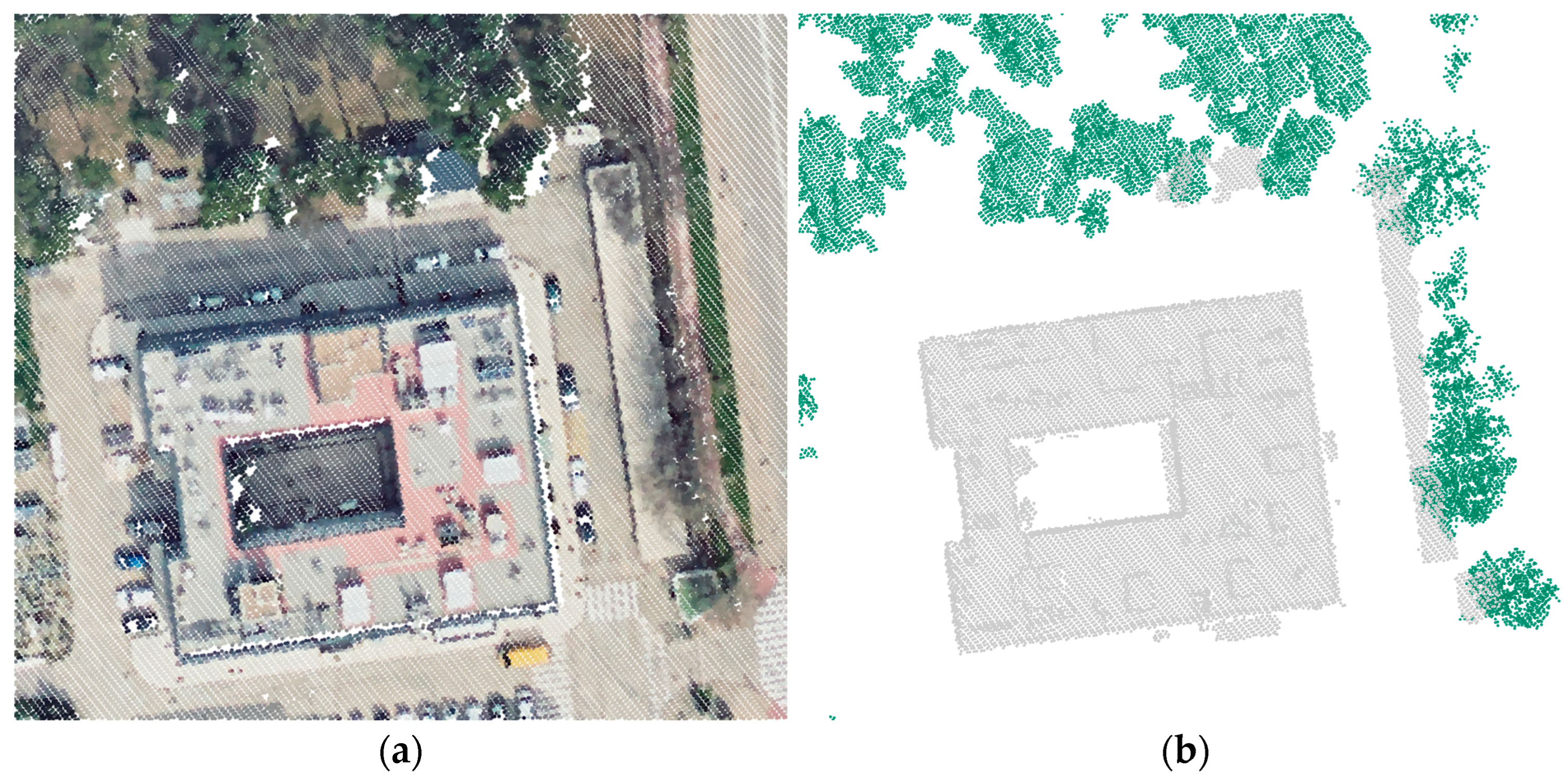
LiDAR data presents some inherent factors to consider. The representativeness of vegetation in LiDAR point clouds, particularly in regard to canopy properties, may be influenced to some extent by the time of the year when data were collected, given the seasonal changes in deciduous foliage. LiDAR flights conducted during leafy seasons should theoretically provide a denser tree canopy status, compared to winter, when deciduous trees are defoliated. To evaluate this effect, Figure 8 shows LiDAR data collected in March 2024 in the vicinity of Building 42, where trees to the north of the building are evergreen and those to the east are deciduous, as seen in the RGB view of LiDAR data. In this comparison, the point cloud classified as high vegetation reveals that both tree types are well represented despite the different foliage.
Figure 8.
Representativeness of evergreen (north of Building 42) and deciduous (east of Building 42) tress in the LiDAR point cloud from March 2024: (a) view with RGB colours; (b) view by classification. (Data source: LiDAR-PNOA-cob2 2024 CC-BY 4.0 scne.es).
Additionally, temporal mismatch between the collection of LiDAR point clouds and the availability of experimental data may lead to significant changes in the surrounding environment (e.g., tree felling, building construction or demolition). If this were the case, LiDAR data should be refined prior to the simulation stage through strategies such as reclassifying points and/or correcting height. For the present case study, no variation in vegetation occurred between 2016 (LiDAR flight) and 2023 (end of the simulated time span).
2.4. Simulation Model Settings and Assumptions in SAM and PVsyst
Table 2 presents the main modelling assumptions adopted in SAM and PVsyst for this study. Mounting configurations were selected among the different options provided by each software tool to best represent the characteristics of the existing ventilated façade. The commercial models of the PV modules and inverters comprising the BIPV systems of Building 42, as laid out in Table 1 earlier, were selected from the built-in libraries in both tools, providing the required specifications for the calculations. The PV layouts were defined according to the electrical configuration of the existing arrays.
Table 2.
Model settings and assumptions in SAM and PVsyst.
Other important calculation parameters include albedo and system losses. Given the urban nature of the surroundings, albedo was assumed to be a standard 0.2 [40]. For wiring and mismatch losses, Table 3 summarises their values and method of acquirement. Snow and ageing losses were considered null, since modules are placed vertically under a Mediterranean climate and were brand new at the time of the building’s renovation, respectively. The remaining system losses were more challenging to address equally in both tools, since each software manages them differently and the information for clarification is limited. Therefore, when the same specific loss parameter was unavailable in both tools, values were set to 0 to avoid inconsistencies.
Table 3.
Assumed normalised values (values over one) for main system losses.
2.5. Calculation of near Shading Losses in SAM and PVsyst
Shading computed with SAM and PVsyst utilises a geometrical analysis of PV modules in relation to their surrounding shading elements. These shading losses can be expressed as the percentage of array surface shaded by obstacles at every timestamp (e.g., 8760 hourly values for a full year) or through the combination of azimuth and height angles of the solar position. SAM follows the first approach by default, while PVsyst utilises the azimuth-to-elevation strategy.
A major difference between both software tools is PVsyst’s capability to read a DSM in various formats: Tagged Image File Format (TIFF), comma-separated values (CSV), or 3D scene from CAD software (3DS, DAE, PVC). SAM, on the other hand, is not able to process these files directly, but allows the replacement of its own shading losses information with files from external sources, such as PVsyst, SunEye or SolarPathfinder.
Consequently, in order to be able to evaluate the DSM in SAM, DSM shading data was calculated previously in PVsyst for each BIPV array, then exported and imported into SAM. This process is performed through the linear shading factor table that PVsyst provides under its near shadings menu. Given that these shading factors are calculated geometrically based on the interaction of the sun’s position in the sky and the obstacles at every azimuth-to-elevation angle combination, which do not vary throughout the years, the same shading table is applicable to each BIPV array in all seven years of simulations. As an example, Table 4 shows the near shading losses factor table for azimuth-to-elevation angle combinations of beam irradiance for the East2 array, obtained with PVsyst through the DSM strategy. Values of 1 mean fully shaded, 0 translates to no shading, and numbers in between indicate different levels of partial shading.
Table 4.
Linear shading factor for the beam component based on solar azimuth-to-elevation angle combinations using a DSM for the East2 array, calculated with PVsyst.
2.6. Generation of Meteorological Data with CAMS and PVGIS
Hourly meteorological input data for simulations were prepared by combining data from CAMS radiation service and PVGIS, and converted to the appropriate format required by each tool. The period 2017–2023 was selected based on the availability of experimental data, beginning in 2017 following the building’s renovation, and meteorological data from PVGIS, which covers the period until 2023. CAMS provides estimations of global horizontal irradiance (GHI), direct normal irradiance (DNI) and diffuse horizontal irradiance (DHI) for total sky and clear sky conditions based on the Heliosat-4 model using Meteosat Second Generation (MSG) satellite imagery [28]. PVGIS also delivers the solar radiation components from MSG satellite images, whereas additional meteorological data, such as temperature and wind speed, are obtained from ERA5 reanalysis [41]. The solar radiation information provided by both services is of high quality; however, recent benchmarking studies reported better accuracy from CAMS radiation service, particularly in DNI [30,32,42]. Therefore, the meteorological input data used for SAM and PVsyst in this work were generated by using the solar radiation components from CAMS and the remaining meteorological variables from PVGIS.
3. Results
The present study involved modelling the energy yield of five BIPV arrays in SAM and PVsyst on an hourly basis for the period 2017–2023, following two different shading-computation strategies: their built-in 3D scene tools and the DSM-derived scene. The input for both tools includes detailed information on the technical parameters of the modules and inverter for each array, façade orientation and shading configuration, the latter being particularly relevant for the east-facing arrays evaluated in this work. The study is developed on an hourly basis, leading to a good level of granularity that enables hourly, daily, monthly and yearly comparisons for an in-depth analysis and better understanding of the system’s behaviour.
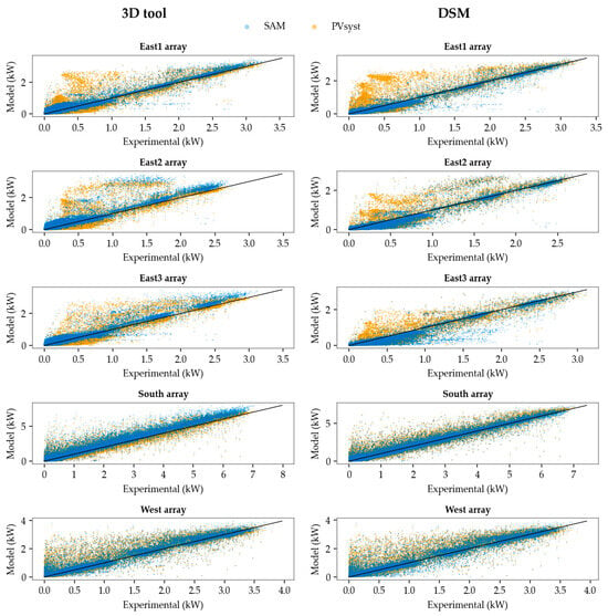
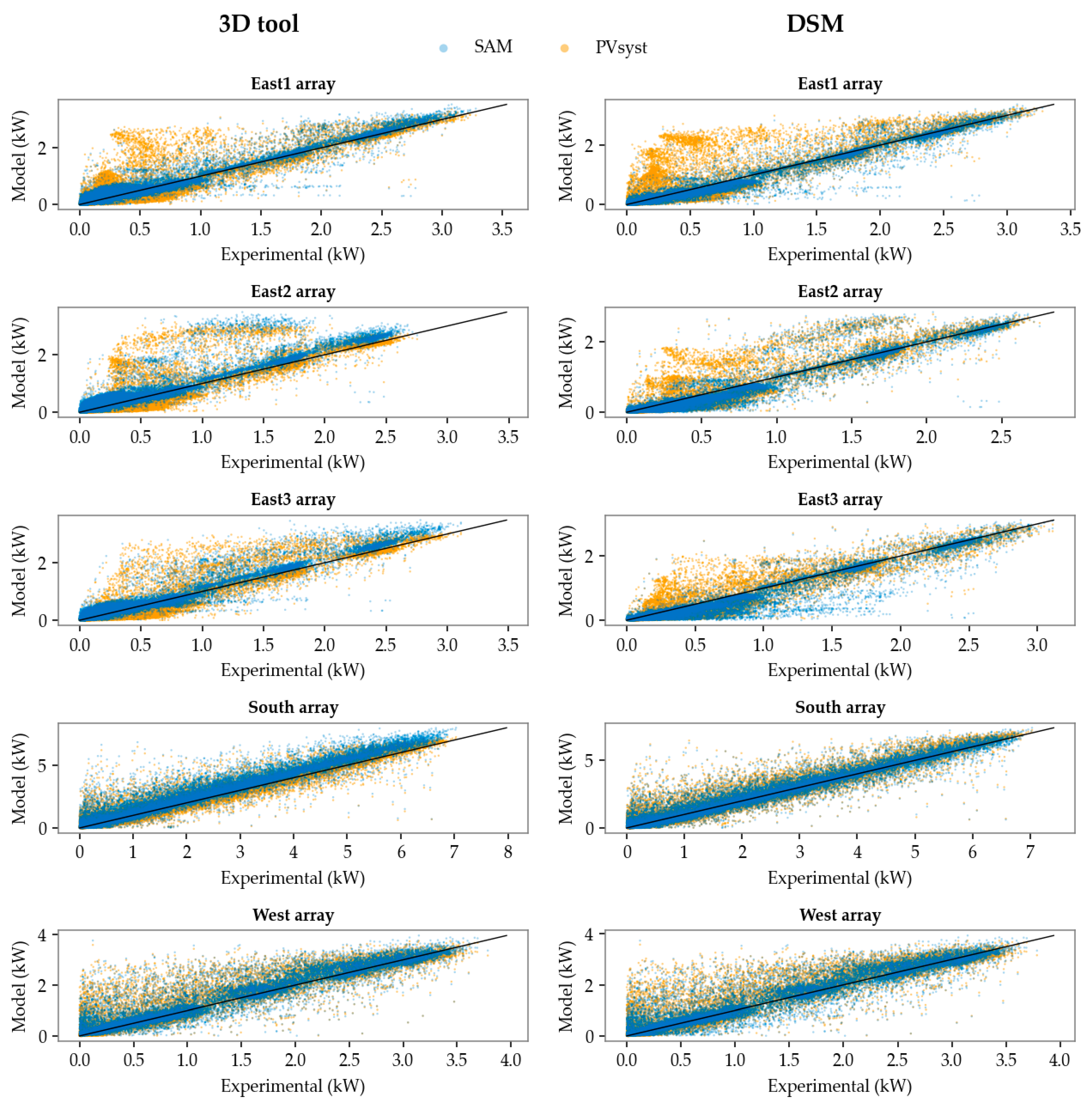
Simulated energy yield hourly results were firstly compared against experimental data in the form of scatter plots (Figure 9) for each array in SAM (blue dots) and PVsyst (yellow dots), as well as the ideal ratio of 1:1 (black line).
Figure 9.
Scatter plots of hourly energy yield values: 3D tool (left) and DSM (right).
These scatter plots show that the simulations for the south and west arrays behave similarly in both software tools, although SAM provides slightly lower dispersion than PVsyst. The difference in performance becomes more apparent for the east arrays, where shading boundary conditions are more complex and difficult to assess. Despite using the same shading configurations in both tools for each of the two modelling strategies (3D tool and DSM), the resulting energy yield estimations differ notably between SAM and PVsyst. These differences likely arise from the way each software tool models shading.
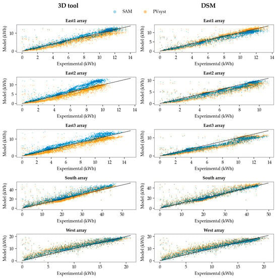
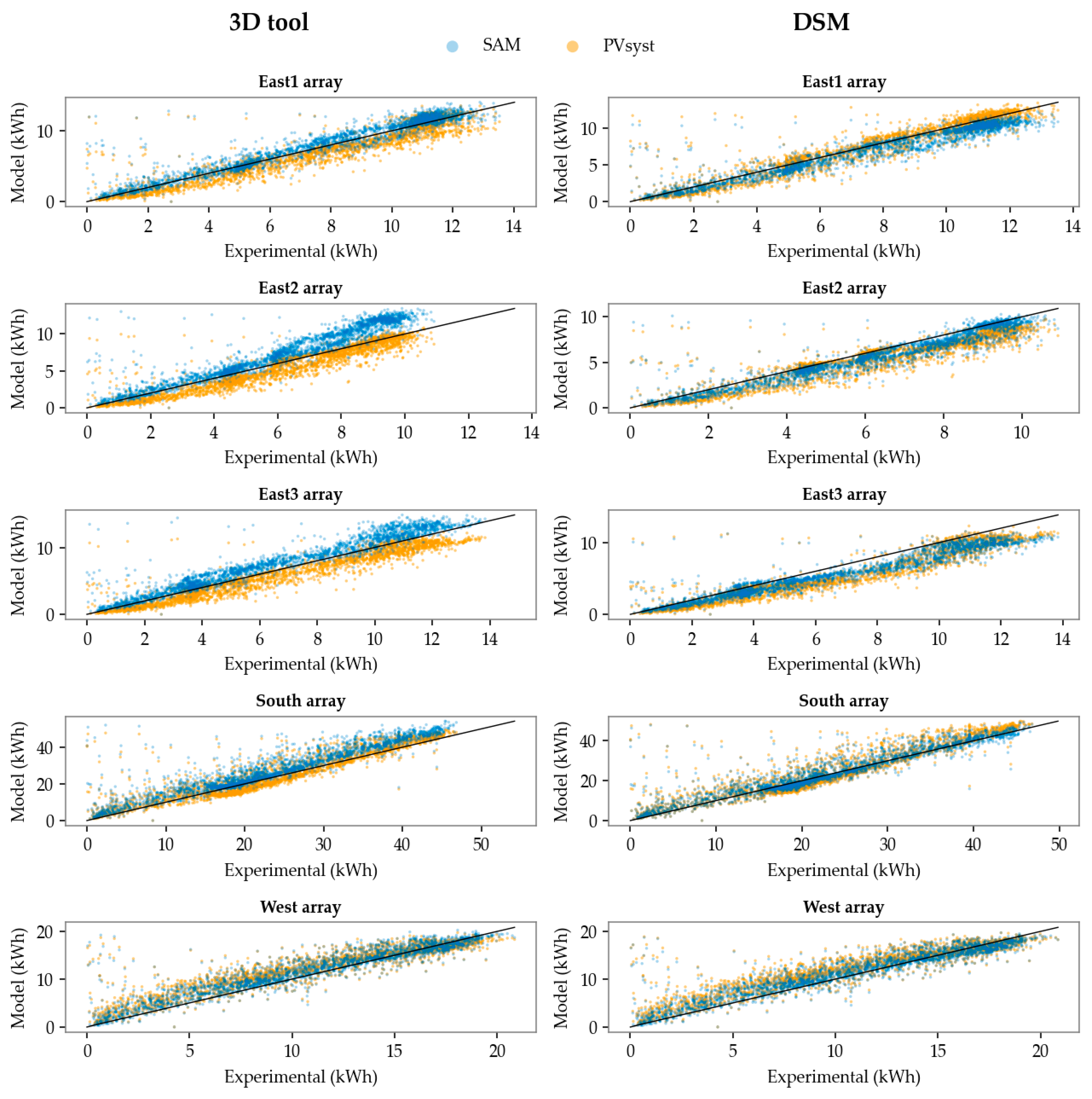
Hourly data poses a challenge to interpret, as it is highly affected by uncertainties that are otherwise dampened over longer time scales. While hourly scatter plots are useful for a granular evaluation and deep understanding of the model’s performance on a smaller time scale, the behaviour of PV systems is more appropriately assessed over long-term periods. Consequently, Figure 10 shows the scatter plots of energy yield daily sums, where simulated values for both software programs outline good behaviour in comparison to experimental data.
Figure 10.
Scatter plots of daily energy yield values: 3D tool (left) and DSM (right).
Deviations from each array are quantified through the mean bias error (MBE), the regular and normalised root mean square errors (RMSE and nRMSE), and the coefficient of determination (R2). It should be noted that these metrics capture different statistical aspects of model performance: MBE quantifies systematic bias, based on the average difference between predicted and observed values that expose the tendency of the model to over- or underestimate; RMSE reflects the overall magnitude of residuals in the form of the standard deviation of prediction errors, leading to large errors and outliers having a high influence in the statistical value; nRMSE normalises the RMSE by the observed mean value; and R2 measures the proportion of the variance in the dependent variable that is explained by the model, i.e., how well observed outcomes are replicated by the model, and may respond differently when the nature of residuals changes. Table 5 and Table 6 show these error metrics when predicting energy yield on a daily basis with SAM and PVsyst, respectively.
Table 5.
Error metrics in modelling daily energy with SAM.
Table 6.
Error metrics in modelling daily energy with PVsyst.
Focusing on RMSE, which integrates systematic and random error components, SAM and PVsyst yield comparable error metrics with both shading strategies. In SAM, the 3D tool provides better results in the East1 and East3 arrays by a small margin, whereas the DSM approach behaves better in the remaining arrays. The difference between the 3D and the DSM is less noticeable in PVsyst, with the 3D tool achieving lower error values in the East2 and East3 arrays and higher in the East1. For the South and West arrays, both strategies offer the same result. Furthermore, MBE values reveal minor over- and underestimation trends in different configurations, as was also observed in the hourly and daily scatterplots.
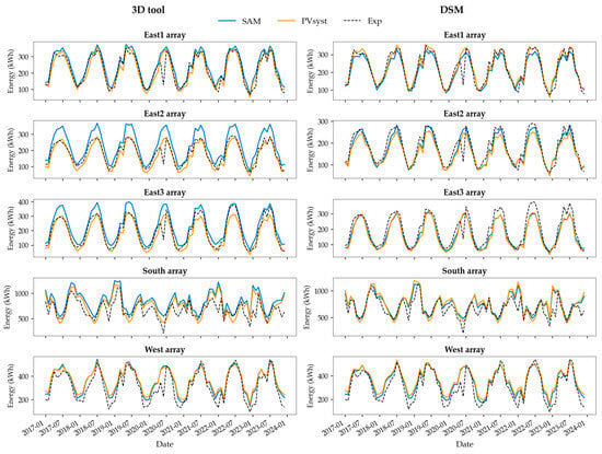
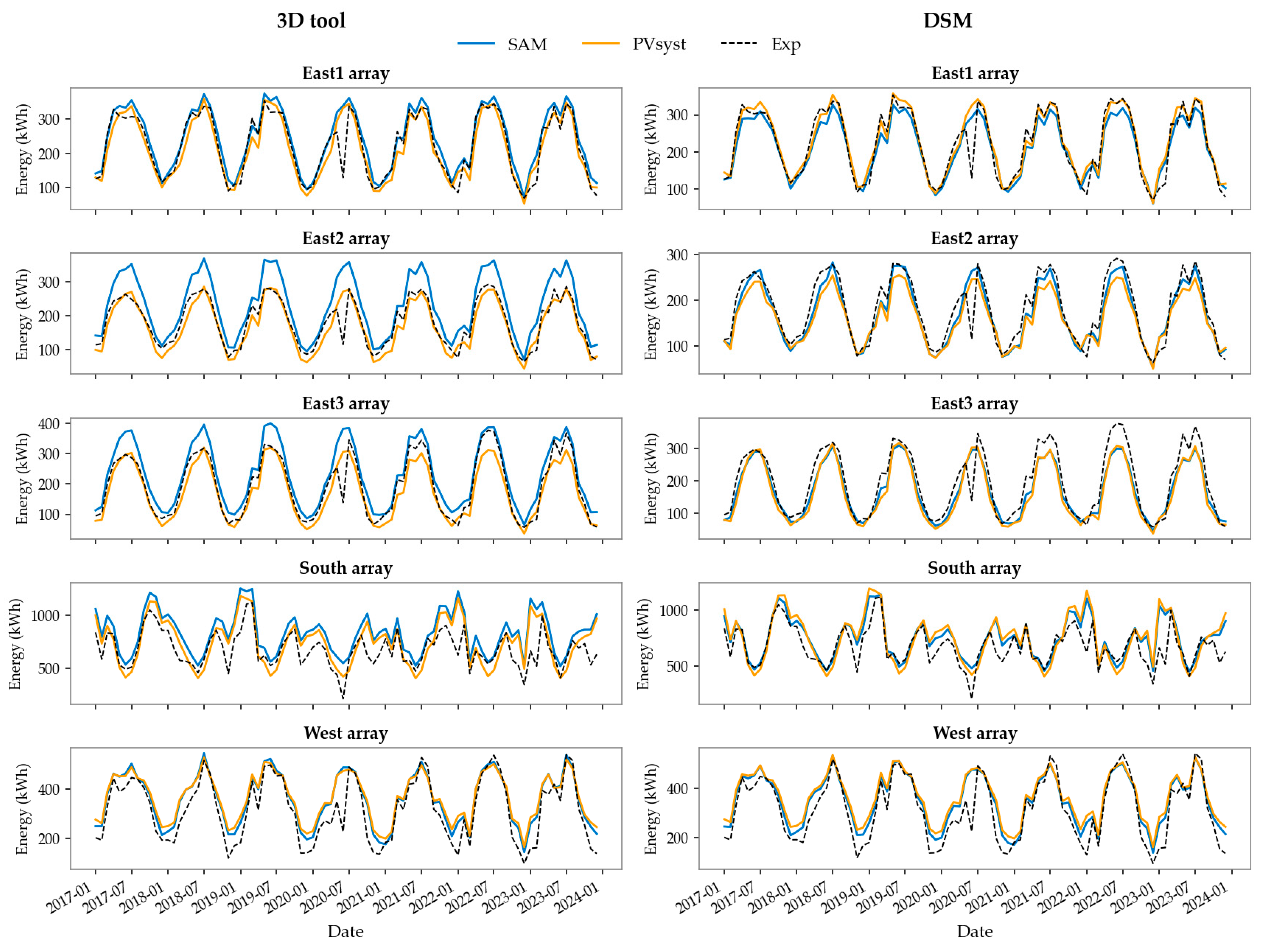
Jumping to a larger time scale, Figure 11 shows the evolution of monthly energy yield computed with SAM (blue line) and PVsyst (yellow line) for all arrays in the seven-year period (2017–2023), compared with experimental data (black dashed line).
Figure 11.
Monthly energy predictions compared with experimental data: 3D tool (left) and DSM (right).
In terms of annual energy yield estimations throughout the seven years studied, it is useful to evaluate the long-term performance and return-on-investment (ROI) of BIPV systems. Table 7 shows the nRMSE values expressed as percentages for the different cases studied. These results show improved performance when using a DSM to assess shading boundary conditions for all arrays in SAM. In PVsyst, the behaviour is similar. The resulting error metrics are consistent with values reported in other benchmarking studies for conventional PV systems [43].
Table 7.
Normalised RMSE for annual energy yield predicted with SAM and PVsyst.
4. Discussion
The results presented in this work analyse the capability of SAM and PVsyst to provide reliable energy yield predictions for BIPV façade applications under different boundary conditions. The uncertainty associated with both PVsyst and SAM in modelling and predicting the energy yield of a BIPV façade is the sum of several contributions: uncertainty in solar irradiance and meteorological data from satellite models and services (in this case, CAMS and PVGIS), uncertainty in the transposition model (e.g., Pérez), uncertainty in PV conversion modelling (based on the simulation models within the software), and uncertainty in modelling PV losses, particularly shading losses (addressed in this paper through the 3D tools and a DSM). Satellite-derived solar irradiance and transposition models are generally accepted and recognised to work with sufficient accuracy in energy yield modelling for PV systems. The contribution to the uncertainty of satellite-based irradiance data has been reported to lie within 2–6% of annual irradiation [44]. The uncertainty in modelling PV conversion losses is low compared to the uncertainty of proper quantification of POA irradiance, which includes shading computation [45]. In addition, benchmarking exercises have proven the overall accuracy of common tools for PV energy yield modelling (including SAM and PVsyst) [43]. Considering these uncertainties, BIPV systems can be effectively modelled by PV modelling tools but require particular attention to properly characterise their specific boundary conditions.
As observed in the error analysis, both the 3D tools and the DSM are suitable to estimate PV energy output in an urban context where shading is significant. When the built-in 3D tools are employed, the main limitation is the need for in situ information to ensure proper building and tree characterisation, data that may be difficult to obtain depending on the circumstances. With this strategy, designing the vegetation requires tree dimensions (i.e., height and canopy diameter) to be estimated from either photos, online resources or in situ observations. If this information cannot be obtained, the usability of this method is limited. Additionally, this procedure can be time-consuming, especially when numerous elements are involved, as they have to be designed individually. From a user perspective, SAM poses an additional challenge when placing BIPV systems in their exact location in the 3D scene, as the view camera is always centred at the origin (0,0,0) and focusing on a specific object becomes more difficult the further it is from this origin.
On the other hand, vegetation defined through a DSM bypasses the need to estimate individual tree size properties, as this information is provided by the LiDAR point cloud, leading to a faster and easily automated procedure. This approach broadens the scope to virtually any location where high quality LiDAR data are available, and is particularly suitable for BIPV projects where in situ vegetation information is difficult to obtain. Limitations in the DSM strategy are related to the availability of LiDAR data, point cloud resolution, and proper point classification, all of which directly influence the accuracy and precision of the DSM. Furthermore, LiDAR information dating back several years may be incomplete or misrepresent the current state of the environment. Having both strategies available ensures that a wide range of BIPV project specifications and requirements can be tackled.
5. Conclusions
The successful deployment of BIPV systems requires demonstrating if existing modelling tools are capable of predicting energy yield with sufficient accuracy. This work explores the use of two common PV modelling tools (SAM and PVsyst) for predicting the energy yield of BIPV façade systems and quantifies the impact of 3D shading characterisation strategies in a case study: a BIPV façade in an urban environment with Mediterranean climate (Madrid, Spain) where experimental energy generation data is available. The study involved modelling five BIPV arrays distributed across three façade orientations during a seven-year period (2017–2023). The resulting errors and uncertainties are consistent with values reported for conventional PV systems, despite the complexities inherent to BIPV. The tools employed have performed reliably, although improvements are still necessary for higher accuracy and better user experience.
This process strongly benefits from openly available information for meteorological conditions and 3D topology. In particular, satellite-derived solar irradiance data—now available for nearly every location worldwide—can be used as the meteorological conditions with high confidence in input data quality. Therefore, when possible, the type of input information used in the models was based on readily available datasets with extensive worldwide coverage, ensuring that the proposed strategy for BIPV energy simulations could be extrapolated to other buildings and locations.
Most challenges associated with modelling BIPV systems can be attributed to boundary conditions that involve shading, particularly within urban contexts where buildings are commonly located. To evaluate this, the present work compares energy yield estimations using the 3D scene created with the built-in tools that SAM and PVsyst provide, and a shading scene derived from a DSM created with GIS analysis using LiDAR data. Because SAM is unable to import the DSM, a near shadings table was calculated in PVsyst and imported into SAM. Overall, energy estimation using the proposed DSM approach provided predicted energy yield values that fell within a similar error range as the built-in 3D tools from each software. In monthly and annual overviews, the DSM shows improvements in SAM. This study remarks that the use a DSM could facilitate energy yield estimations in cases affected by shading where in situ data is insufficient or missing, particularly in regard to trees and vegetation.
The procedures and approaches shown in this paper outline the good behaviour of two conventional PV tools for BIPV applications if shading boundary conditions are properly addressed. These results can support decision-making in BIPV implementations. Furthermore, the proposed DSM methodology is promising for certain applications, and its good behaviour encourages further research across different locations to enable a deeper evaluation under varying environmental conditions.
Author Contributions
Conceptualization, A.M.-C., N.M.-C. and J.P.; methodology, A.M.-C., N.M.-C. and J.P.; software, A.M.-C. and J.P.; validation, A.M.-C., N.M.-C., C.S.-S. and J.P.; formal analysis, A.M.-C., N.M.-C. and J.P.; investigation, A.M.-C., N.M.-C., C.S.-S. and J.P.; resources, A.M.-C., N.M.-C., C.S.-S. and J.P.; data curation, A.M.-C., N.M.-C., C.S.-S. and J.P.; writing—original draft preparation, A.M.-C. and J.P.; writing—review and editing, A.M.-C., N.M.-C., C.S.-S. and J.P.; visualisation, A.M.-C. and J.P.; supervision, N.M.-C. and J.P.; project administration, N.M.-C. and J.P.; funding acquisition, N.M.-C. and J.P. All authors have read and agreed to the published version of the manuscript.
Funding
This publication is part of the R + D + I project “RINGS-BIPV Project (PID2021-124910OB-C31)”, which is funded by the MICIU/AEI/10.13039/5011000011033 and by ERDF/EU.
Data Availability Statement
Data are available upon request.
Acknowledgments
The authors acknowledge the collaborative work conducted under the International Energy Agency Photovoltaic Power Systems Programme (IEA-PVPS) Task 15: Enabling Framework for the Development of BIPV, and Task 16: Solar Resource for High Penetration and Large Scale Applications, in which they actively participate.
Conflicts of Interest
The authors declare no conflicts of interest.
Abbreviations
The following abbreviations are used in this manuscript:
| BAPV | Building-Attached Photovoltaics |
| BIPV | Building-Integrated Photovoltaics |
| CAMS | Copernicus Atmosphere Monitoring System |
| DSM | Digital Surface Model |
| GIS | Geographic Information System |
| IEA | International Energy Agency |
| LiDAR | Light Detection and Ranging |
| MBE | Mean Bias Error |
| MSG | Meteosat Second Generation |
| NSRDB | National Solar Radiation Data Base |
| POA | Plane Of the Array |
| PV | Photovoltaic, Photovoltaics |
| PVGIS | Photovoltaic Geographical Information System |
| PVPS | Photovoltaic Power Systems Programme |
| RMSE | Root Mean Square Error |
| SAM | System Advisor Model |
References
- European Commission Fit for 55: Delivering the EU’s 2030 Climate Target on the Way to Climate Neutrality. 2021. Available online: https://eur-lex.europa.eu/legal-content/EN/TXT/PDF/?uri=CELEX:52021DC0550 (accessed on 13 April 2026).
- European Parliament and Council of the European Union Directive (EU). 2023/1791 of the European Parliament and of the Council of 13 September 2023 on Energy Efficiency and Amending Regulation (EU) 2023/955 (Recast); EU: Brussels, Belgium, 2023. [Google Scholar]
- European Parliament and Council of The European Union Directive (EU). 2024/1275 of the European Parliament and of the Council of 24 April 2024 on the Energy Performance of Buildings; EU: Brussels, Belgium, 2024. [Google Scholar]
- Martín-Chivelet, N.; van Noord, M.; Tilli, F.; Yang, R.J.; Weerasinghe, N.; Daun, E.; Baggini, A. BIPV Market Development: International Technological Innovation System Analysis. Buildings 2025, 15, 3011. [Google Scholar] [CrossRef] [Scilit]
- Valckenborg, R.; Gaisberger, L.; Berger, K.A.; Gusztáv, Ú.; Eder, G.C.; Illich, P.; López, C.S.P.; Boddaert, S.; del Buono, M.; Chivelet, N.M.; et al. Successful Building Integration of Photovoltaics—A Collection of International Projects; IEA-PVPS TCP Task 15: Redfern, NSW, Australia, 2021. [Google Scholar]
- Shahverdian, M.H.; Najaftomaraei, M.; Fassadi Chimeh, A.; Yavarzadeh, N.; Sohani, A.; Javadijam, R.; Sayyaadi, H. Towards Zero-Energy Buildings: A Comparative Techno-Economic and Environmental Analysis of Rooftop PV and BIPV Systems. Buildings 2025, 15, 999. [Google Scholar] [CrossRef] [Scilit]
- Parolini, F.; Bonomo, P.; Frontini, F.; Bellenda, G.; Caccivio, M.; Federova, A.; Boddaert, S.; Chivelet, N.M.; Wilson, H.R. Advancing BIPV Standardization: Addressing Regulatory Gaps and Performance Challenges; Report IEA-PVPS T15-24:2024; IEA-PVPS TCP Task 15: Redfern, NSW, Australia, 2024. [Google Scholar]
- Chivelet, N.M.; Kapsis, C.; Frontini, F. Building-Integrated Photovoltaics; Routledge: Oxfordshire, UK, 2024. [Google Scholar]
- Chen, L.; Baghoolizadeh, M.; Basem, A.; Ali, S.H.; Ruhani, B.; Sultan, A.J.; Salahshour, S.; Alizadeh, A. A Comprehensive Review of a Building-Integrated Photovoltaic System (BIPV). Int. Commun. Heat Mass Transf. 2024, 159, 108056. [Google Scholar] [CrossRef] [Scilit]
- Shukla, A.K.; Sudhakar, K.; Baredar, P. Recent Advancement in BIPV Product Technologies: A Review. Energy Build. 2017, 140, 188–195. [Google Scholar] [CrossRef] [Scilit]
- Kaaya, I.; Alzade, A.; Bouguerra, S.; Kyranaki, N. A Physics-Based Framework for Modelling the Performance and Reliability of BIPV Systems. Sol. Energy 2024, 277, 112730. [Google Scholar] [CrossRef] [Scilit]
- Freitas, J.d.S.; Cronemberger, J.; Soares, R.M.; Amorim, C.N.D. Modeling and Assessing BIPV Envelopes Using Parametric Rhinoceros Plugins Grasshopper and Ladybug. Renew. Energy 2020, 160, 1468–1479. [Google Scholar] [CrossRef] [Scilit]
- Yang, R.J.; Imalka, S.T.; Wijeratne, W.M.P.; Amarasinghe, G.; Weerasinghe, N.; Jayakumari, S.D.S.; Zhao, H.; Wang, Z.; Gunarathna, C.; Perrie, J.; et al. Digitalizing Building Integrated Photovoltaic (BIPV) Conceptual Design: A Framework and an Example Platform. Build. Environ. 2023, 243, 110675. [Google Scholar] [CrossRef] [Scilit]
- Yang, R.J.; Zhao, Y.; Jayakumari, S.D.S.; Schneider, A.; Rajan, S.P.; Leloux, J.; Alamy, P.; Raharjo, G.P.; Rende, F.; Samarasinghalage, T.; et al. Digitalising BIPV Energy Simulation: A Cross Tool Investigation. Energy Build. 2024, 318, 114484. [Google Scholar] [CrossRef] [Scilit]
- Prieto, I.; Izkara, J.L.; Usobiaga, E. The Application of Lidar Data for the Solar Potential Analysis Based on Urban 3D Model. Remote Sens. 2019, 11, 2348. [Google Scholar] [CrossRef] [Scilit]
- Brito, M.C.; Freitas, S.; Guimarães, S.; Catita, C.; Redweik, P. The Importance of Facades for the Solar PV Potential of a Mediterranean City Using LiDAR Data. Renew. Energy 2017, 111, 85–94. [Google Scholar] [CrossRef] [Scilit]
- Polo, J.; Martín-Chivelet, N.; Sanz-Saiz, C. BIPV Modeling with Artificial Neural Networks: Towards a BIPV Digital Twin. Energies 2022, 15, 4173. [Google Scholar] [CrossRef] [Scilit]
- Polo, J.; Martín-Chivelet, N.; Alonso-Abella, M.; Alonso-García, C. Photovoltaic Generation on Vertical Façades in Urban Context from Open Satellite-Derived Solar Resource Data. Sol. Energy 2021, 224, 1396–1405. [Google Scholar] [CrossRef] [Scilit]
- Liang, J.; Gong, J.; Zhou, J.; Ibrahim, A.N.; Li, M. An Open-Source 3D Solar Radiation Model Integrated with a 3D Geographic Information System. Environ. Model. Softw. 2015, 64, 94–101. [Google Scholar] [CrossRef] [Scilit]
- Li, Q.; Yang, G.; Bian, C.; Long, L.; Wang, X.; Gao, C.; Lam, C.; Huang, Y.; Zhao, B.; Chen, X.; et al. Autonomous Design Framework for Deploying Building Integrated Photovoltaics. Appl. Energy 2025, 377, 124760. [Google Scholar] [CrossRef] [Scilit]
- Sow, M.C.; Pv, B.I. Energy & Buildings BI 2 PV Simulator for Optimized BIPV Design in Industrial Buildings. Energy Build. 2026, 350, 116576. [Google Scholar]
- Zheng, S.; Bai, J.; Akram, M.W. An Enhanced Method for Design and Simulation of Building Integrated Photovoltaic Plants Incorporating Photovoltaic Resource Assessment. Build. Simul. 2025, 18, 1087–1101. [Google Scholar] [CrossRef] [Scilit]
- Urraca, R.; Gracia-Amillo, A.M.; Koubli, E.; Huld, T.; Trentmann, J.; Riihelä, A.; Lindfors, A.V.; Palmer, D.; Gottschalg, R.; Antonanzas-Torres, F. Extensive Validation of CM SAF Surface Radiation Products over Europe. Remote Sens. Environ. 2017, 199, 171–186. [Google Scholar] [CrossRef] [Scilit]
- Huld, T.; Müller, R.; Gambardella, A. A New Solar Radiation Database for Estimating PV Performance in Europe and Africa. Sol. Energy 2012, 86, 1803–1815. [Google Scholar] [CrossRef] [Scilit]
- Huld, T.; Paietta, E.; Zangheri, P.; Pinedo Pascua, I. Assembling Typical Meteorological Year Data Sets for Building Energy Performance Using Reanalysis and Satellite-Based Data. Atmosphere 2018, 9, 53. [Google Scholar] [CrossRef] [Scilit]
- Gschwind, B.; Wald, L.; Blanc, P.; Lefèvre, M.; Schroedter-Homscheidt, M.; Arola, A. Improving the McClear Model Estimating the Downwelling Solar Radiation at Ground Level in Cloud-Free Conditions—McClear-V3. Meteorol. Z. 2019, 28, 147–163. [Google Scholar] [CrossRef] [Scilit]
- Schroedter-Homscheidt, M.; Azam, F.; Betcke, J.; Hanrieder, N.; Lefèvre, M.; Saboret, L.; Saint-Drenan, Y.M. Surface Solar Irradiation Retrieval from MSG/SEVIRI Based on APOLLO Next Generation and HELIOSAT-4 Methods. Meteorol. Z. 2022, 31, 455–476. [Google Scholar] [CrossRef] [Scilit]
- Qu, Z.; Oumbe, A.; Blanc, P.; Espinar, B.; Gesell, G.; Gschwind, B.B.; Klüser, L.; Lefèvre, M.; Saboret, L.; Schroedter-Homscheidt, M.; et al. Fast Radiative Transfer Parameterisation for Assessing the Surface Solar Irradiance: The Heliosat-4 Method. Meteorol. Z. 2017, 26, 33–57. [Google Scholar] [CrossRef] [Scilit]
- Sengupta, M.; Xie, Y.; Lopez, A.; Habte, A.; Maclaurin, G.; Shelby, J. The National Solar Radiation Data Base (NSRDB). Renew. Sustain. Energy Rev. 2018, 89, 51–60. [Google Scholar] [CrossRef] [Scilit]
- Yang, D.; Bright, J.M. Worldwide Validation of 8 Satellite-Derived and Reanalysis Solar Radiation Products: A Preliminary Evaluation and Overall Metrics for Hourly Data over 27 Years. Sol. Energy 2020, 210, 3–19. [Google Scholar] [CrossRef] [Scilit]
- Yang, D. A Correct Validation of the National Solar Radiation Data Base (NSRDB). Renew. Sustain. Energy Rev. 2018, 97, 152–155. [Google Scholar] [CrossRef] [Scilit]
- Lund, H. Worldwide Benchmark of Modelled Solar Irradiance Data 2023; IEA PVPS Task 16: Redfern, NSW, Australia, 2023. [Google Scholar]
- Gilman, P.; Dobos, A.; Diorio, N.; Freeman, J.; Janzou, S.; Ryberg, D. SAM Photovoltaic Model Technical Reference Update; NREL: Golden, CO, USA, 2016.
- Mermoud, A.A.; Wittmer, B. Pvsyst User’s Manual; PVSYST SA: Satigny, Switzerland, 2014. [Google Scholar]
- Marcos-Castro, A.; Martín-Chivelet, N.; Polo, J. Enhanced GIS Methodology for Building-Integrated Photovoltaic Façade Potential Based on Free and Open-Source Tools and Information. Remote Sens. 2025, 17, 954. [Google Scholar] [CrossRef] [Scilit]
- Lindberg, F.; Jonsson, P.; Honjo, T.; Wästberg, D. Solar Energy on Building Envelopes—3D Modelling in a 2D Environment. Sol. Energy 2015, 115, 369–378. [Google Scholar] [CrossRef] [Scilit]
- Konarska, J.; Lindberg, F.; Larsson, A. Transmissivity of Solar Radiation through Crowns of Single Urban Trees—Application for Outdoor Thermal Comfort Modelling. Theor. Appl. Clim. 2014, 117, 363–376. [Google Scholar] [CrossRef] [Scilit]
- Perez, R.; Ineichen, P.; Seals, R.; Michalsky, J.; Stewart, R. Modeling Daylight Availability and Irradiance Components from Direct and Global Irradiance. Sol. Energy 1990, 44, 271–289. [Google Scholar] [CrossRef] [Scilit]
- Duffie, J.A.; Beckman, W.A. Solar Engineering of Thermal Processes; John Wiley & Sons: Hoboken, NJ, USA, 2013. [Google Scholar]
- Polo, J.; Sanz-saiz, C. Development of Spectral Mismatch Models for BIPV Applications in Building Façades Abbreviations. Renew. Energy 2025, 245, 122820. [Google Scholar] [CrossRef] [Scilit]
- Urraca, R.; Huld, T.; Lindfors, A.V.; Riihelä, A.; Martinez-de-Pison, F.J.; Sanz-Garcia, A. Quantifying the Amplified Bias of PV System Simulations Due to Uncertainties in Solar Radiation Estimates. Sol. Energy 2018, 176, 663–677. [Google Scholar] [CrossRef] [Scilit]
- Verbois, H.; Saint-Drenan, Y.-M.; Becquet, V.; Gschwind, B.; Blanc, P. Retrieval of Surface Solar Irradiance from Satellite Imagery Using Machine Learning: Pitfalls and Perspectives. Atmos. Meas. Tech. 2023, 16, 4165–4181. [Google Scholar] [CrossRef] [Scilit]
- Theristis, M.; Deville, L.; Ovaitt, S.; Stein, J.S.; Micheli, L.; Driesse, A.; Hobbs, W.B.; Daxini, R.; Barrie, D.; Campanelli, M.; et al. Blind Photovoltaic Modeling Intercomparison: A Multidimensional Data Analysis and Lessons Learned. Prog. Photovolt. 2023, 31, 1049–1157. [Google Scholar] [CrossRef] [Scilit]
- Moser, D.; Lindig, S.; Richter, M.; Asencio-Vasquez, J.; Horvath, I.; Müller, B.; Green, M.; Vedde, J.; Herz, M.; Herteleer, B.; et al. Uncertainties in Yield Assessments and PV LCOE; Report IEA-PVPS T13-18; IEA PVPS Task 13: Redfern, NSW, Australia, 2020. [Google Scholar]
- Reise, C.; Müller, B.; Driesse, A.; Razongles, G.; Richter, M. Uncertainties in PV System Yield Predictions and Assessments; Report IEA-PVPS T13-12; IEA PVPS Task 13: Redfern, NSW, Australia, 2018. [Google Scholar]

Disclaimer/Publisher’s Note: The statements, opinions and data contained in all publications are solely those of the individual author(s) and contributor(s) and not of MDPI and/or the editor(s). MDPI and/or the editor(s) disclaim responsibility for any injury to people or property resulting from any ideas, methods, instructions or products referred to in the content. |
© 2026 by the authors. Licensee MDPI, Basel, Switzerland. This article is an open access article distributed under the terms and conditions of the Creative Commons Attribution (CC BY) license.