


Abstract
The performance-based seismic design of fluid viscous dampers (FVDs) for long-span cable-stayed bridges was fundamentally challenged by prohibitive computational costs and the lack of generalizable methodologies. This study proposed a transfer learning-based hybrid surrogate modeling framework for efficient multi-objective seismic design. High-fidelity models of three representative bridges were developed to generate a comprehensive seismic response database. A systematic comparison identified the Radial Basis Function Network (RBFN) as the optimal core surrogate model. The pivotal innovation was a transfer learning strategy, enabling a pre-trained RBFN model to be rapidly and accurately adapted to a new bridge design with minimal additional data. This adapted RBFN was integrated with a Kriging model to form a hybrid surrogate, which was embedded within an NSGA-II optimization loop to efficiently identify the Pareto-optimal set of FVD parameters. The robustness and performance gains of the optimized designs were rigorously validated through high-fidelity simulation. The proposed framework reduces the computational cost of the design cycle by approximately two orders of magnitude (from 1700 to 50 CPU-hours), providing a practical and reusable pathway for the seismic design of long-span cable-stayed bridges.
1. Introduction
The evolution of cable-stayed bridges (CSB) into the kilometer-span regime marks a pinnacle of modern civil engineering, driven by socioeconomic demands and technological breakthroughs. These graceful yet formidable structures now routinely conquer geographic barriers once deemed impassable, enabling direct transportation links across wide waterways and deep gorges. However, this leap in span introduces a fundamental conflict: the slender, lightweight configurations that enable such achievements also amplify their susceptibility to dynamic environmental actions, with seismic hazards representing a paramount design concern [1,2,3].
The inherent seismic vulnerability of super-long-span cable-stayed bridges is primarily attributed to their elongated natural periods. These periods often resonate with the velocity- and displacement-sensitive spectral bands of earthquake ground motions, especially for far-field events with substantial long-period energy content [4]. Under strong shaking, these bridges exhibit intricate dynamic coupling among longitudinal, transverse, and torsional modes, compounded by cable-structure interaction and potential geometric nonlinearities [5]. Unmitigated seismic responses can trigger catastrophic scenarios, including excessive deck displacements leading to unseating, perilously high internal forces in pylons and piers, and damaging stress fluctuations in stay cables [6,7]. Given their role as critical lifelines, ensuring the seismic resilience of these megastructures is a profound societal imperative that demands performance-based design philosophies exceeding prescriptive code requirements [8].
To fulfill this imperative, supplemental energy dissipation has become integral to the seismic design of long-span bridges. Among various devices, Fluid Viscous Dampers (FVDs) stand out due to their effectiveness and reliability [9]. Installed typically between the deck and towers, FVDs generate an out-of-phase damping force that follows a nonlinear constitutive law, , where is the damping coefficient and is the velocity exponent. This mechanism enables significantly reducing displacements and accelerations without substantially increasing structural stiffness, thereby avoiding higher inertial force attraction [10,11,12]. The successful deployment of FVDs in iconic bridges worldwide validates their status as a premier seismic protection strategy [13].
Nevertheless, the performance of an FVD is critically contingent upon the optimal selection of its parameters (C, α). This selection constitutes a complex multi-objective optimization problem [14]. Key objectives include minimizing structural responses (e.g., deck displacement, pylon base moment) and simultaneously controlling device demands (e.g., damper force, stroke), which dictate cost and feasibility [15]. These objectives are intrinsically conflicting; for instance, a high C value may drastically reduce displacements but yield impractically large damper forces. The velocity exponent α further modulates this trade-off across different velocity regimes. Consequently, the optimal design solution is not a single point but a set of Pareto-optimal solutions representing the best possible compromises [16,17].
Conventional design practice navigates this trade-off through parametric studies, guided by engineering experience and supported by iterative Nonlinear Time-History Analysis (NLTHA). This process involves executing numerous computationally intensive, high-fidelity finite element simulations across different (C, α) pairs under a suite of ground motions [18]. While feasible for specific cases, this approach faces two major bottlenecks [19]. First, the computational expense is prohibitive for exhaustive exploration. A single detailed NLTHA for a kilometer-scale bridge can consume hours; exploring the continuous 2D parameter space under multiple seismic scenarios is often intractable within project constraints. Second, the process is intrinsically structure-specific. Optimal parameters for one bridge, dictated by its unique dynamic fingerprint, offer little direct insight for another, necessitating a complete and costly re-analysis for each new project [20]. This lack of generalizability hinders the development of transferable design knowledge.
Before presenting the proposed methodology, it is essential to clarify the modeling philosophy underpinning this study regarding structural nonlinearity. In long-span cable-stayed bridges, the tall main tower exhibits limited ductility capacity, and the formation of plastic hinges at the tower base would lead to substantial residual displacements at the tower top, making post-earthquake repair extremely challenging and economically prohibitive [3]. Consequently, it is a widely accepted design principle, consistent with capacity design philosophy and seismic design codes [21], that the primary load-bearing components, particularly the main tower, should remain essentially elastic under design earthquake actions. Seismic mitigation strategies therefore focus on reducing dynamic response through energy dissipation devices such as FVDs, which act as sacrificial elements to protect the main structure. Extreme events exceeding design intensities may lead to structural collapse, but such scenarios fall beyond the scope of current seismic design codes. Following this engineering rationale, the present study adopts a modeling approach that respects these constraints while explicitly capturing the dominant sources of structural nonlinearity—namely, geometric nonlinearity arising from dead-load-induced stiffness and the intrinsic nonlinear behavior of FVDs. A detailed description of the nonlinear modeling framework is provided in Section 2.2.3.
The field of performance-based earthquake engineering has increasingly embraced surrogate modeling (metamodeling) to overcome computational bottlenecks [22]. Surrogate models are fast-to-evaluate mathematical emulators trained on a finite set of high-fidelity simulation data. Techniques like Artificial Neural Networks (ANNs) [23], Kriging (Gaussian Process Regression) [24,25], and Support Vector Regression [26] have proven effective for seismic demand prediction and reliability analysis. Once trained, these models can evaluate thousands of design scenarios in seconds, liberating optimization algorithms from direct dependence on expensive simulations. This enables the application of advanced multi-objective evolutionary algorithms like NSGA-II [27,28,29] for thorough design space exploration. Surrogate-assisted optimization has shown promise in related problems, such as tuning Tuned Mass Dampers [30].
A persistent and critical gap, however, remains: current surrogate models are predominantly developed for a single, fixed structural configuration. A model meticulously trained on Bridge A’s response database typically fails to generalize to Bridge B without being retrained on a comparably large new dataset [31]. This limitation forfeits a key potential advantage of data-driven methods—knowledge transfer and reuse across related problems. Transfer Learning (TL), a subfield of machine learning, provides a powerful framework to bridge this gap [32]. TL techniques enhance learning in a data-scarce target domain by leveraging knowledge from a related, data-rich source domain. Early applications in civil engineering, such as adapting damage detection models or predicting seismic responses of buildings with limited data [33], demonstrate its potential. The core strategy involves taking a model pre-trained on a source structure and efficiently adapting (“fine-tuning”) it using a small, targeted dataset from a new structure.
Converging these technological strands—high-fidelity simulation, surrogate modeling, transfer learning, and efficient optimization—this study proposes a novel, integrated framework for the seismic design of FVDs in kilometer-scale cable-stayed bridges. The framework introduces two primary innovations: (1) a transfer learning protocol that enables rapid adaptation of surrogate models across different bridge designs with minimal data, effectively breaking the “one-structure, one-model” paradigm; and (2) a hybrid RBFN-Kriging surrogate that combines fast prediction with uncertainty quantification to enhance the robustness of multi-objective optimization. By integrating these innovations, the proposed methodology is architected to be both computationally efficient and inherently generalizable, accumulating knowledge from past projects and accelerating the convergence to high-performance solutions for new designs.
This study frames its performance objectives within the context of widely adopted seismic design codes and guidelines. The modeling approach follows capacity design principles as prescribed in ASCE/SEI 7-22 [34], which requires critical structural elements to maintain elastic behavior during design-level seismic events for Risk Category III structures. For the specific case of long-span cable-stayed bridges, the ASCE design guidelines [35] offer detailed provisions on seismic considerations, including material requirements and performance criteria. The assumption that the main tower remains elastic under design-basis earthquakes—a fundamental premise of this work—is also consistent with the philosophy underlying China’s urban bridge seismic code [21], where post-earthquake repairability of key components is prioritized. By embedding the proposed optimization framework within this codified context, the resulting damper configurations are positioned to satisfy both numerical optimization objectives and practical design expectations.
2. Methodology: The Proposed Framework
2.1. Overall Framework Schematic
The overarching architecture of the proposed framework is depicted in Figure 1. It is structured into three sequential, interdependent phases, ensuring a systematic progression from data generation to verified design solutions.
Figure 1.
Schematic of the integrated framework for surrogate-assisted multi-objective optimization of FVD parameters.
Phase I establishes the foundation through high-fidelity finite element modeling of two distinct kilometer-scale cable-stayed bridges (M1, M2). A comprehensive seismic response database is constructed by performing batch nonlinear time-history analyses across a systematically sampled input space of ground motion intensities and FVD parameters (C, α).
Phase II focuses on developing intelligent, reusable predictive models. The database is used to train and compare multiple neural network surrogates, with the Radial Basis Function Network (RBFN) identified as optimal. A core innovation of this phase is the transfer learning protocol, which is rigorously tested by applying the M1-trained RBFN model to predict responses for bridges M2, observing a predictable performance decline. This decline is effectively remedied by fine-tuning the pre-trained model with a minimal amount of new target-bridge data, demonstrating rapid adaptation. The validated, transferable RBFN model is then coupled with a Kriging model to form a hybrid surrogate that delivers both high-speed predictions and essential uncertainty estimates.
Phase III leverages this hybrid surrogate within a multi-objective optimization (MOO) loop. The NSGA-II algorithm, integrated with the surrogate, efficiently explores the design space to identify the Pareto-optimal frontier, trading off structural performance (e.g., deck displacement) against damper demand (e.g., damper force). Finally, selected optimal solutions from the Pareto set are validated by back-substitution into the original high-fidelity FEM, closing the verification loop and yielding the final, reliable FVD design parameters.
This closed-loop framework explicitly addresses the dual challenges of computational efficiency (via surrogate modeling and efficient optimization) and generalizability (via the embedded transfer learning strategy), advancing beyond conventional structure-specific design approaches.
2.2. High-Fidelity Finite Element Modeling and Validation
2.2.1. Prototype Bridge Descriptions
1. Baseline Model-M1
An extra-large span cable-stayed bridge has a total length of 2088 m with seven spans. Its main girder is a continuous steel box girder with a span arrangement of 2 × 100 + 300 + 1088 + 300 + 2 × 100 m, as shown in Figure 2. The inverted Y-shaped reinforced concrete pylon stands 297.7 m tall. The upper pylon section houses the stay cable zone, while the middle and lower sections comprise two separate inclined pylons. A lower crossbeam connects the tower columns at the tower-girder junction. The tower foundations employ a pile cap foundation system. The piers include near-tower auxiliary piers, far-tower auxiliary piers, and transition piers, with heights averaging approximately 60 m. Longitudinal sliding bearings are installed at the pier tops.
Figure 2.
Bridge longitudinal profile of Basic Model -M1(unit: meters).
2. Derived Model M2
Based on the foundational model, a kilometer-scale CSB with a main span of 1500 m was designed and simulated. The CSB has a total length of 2876 m with seven spans. Its main girder is a continuous steel box girder with a span arrangement of 2 × 138 + 412 + 1500 + 412 + 2 × 138 m, as shown in Figure 3. The inverted Y-shaped reinforced concrete pylon stands 370 m tall.The remaining design details of this model are identical to those of the basic model.
Figure 3.
Bridge longitudinal profile of imitation design model-M2 (unit: meters).
3. Derived Model M3
Additionally, another kilometer-scale CSB with a main span of 1900 m was also designed and simulated based on the basic model. The CSB has a total length of 3850 m with seven spans. Its main girder is a continuous steel box girder with a span arrangement of 3 × 175 + 450 + 1900 + 450 + 4 × 175 m, as shown in Figure 4. The inverted Y-shaped reinforced concrete pylon stands 492 m tall. The remaining design details of this model are identical to those of the basic model.
Figure 4.
Bridge longitudinal profile of imitation design model2 (unit: meters).
4. Summary of Bridge Configurations
It is important to note that Bridges M2 and M3 are not independent designs but rather scaled-up variants following the same design philosophy as the basic model M1. This systematic scaling approach—where key parameters such as main span length, tower height, and total mass are proportionally increased while maintaining consistent structural form (inverted Y-shaped towers, continuous steel box girder, longitudinal sliding bearings)—creates a family of bridges with progressively increasing flexibility. As shown in Table 1, the fundamental periods range from 15.24 s for the 1088 m main span (M1) to 21.83 s for the 1500 m main span (M2) and 27.62 s for the 1900 m main span (M3). This systematic variation in dynamic characteristics makes the three configurations ideal for testing the generalizability of the proposed optimization framework across a representative spectrum of long-span cable-stayed bridges, from the established 1000 m class to the emerging 2000 m class.
Table 1.
Key structural parameters of the three bridge configurations.
To quantify the structural similarity between the source bridge (M1) and target bridges (M2, M3), we compare their first five natural frequencies. The average relative differences are 12.4% for M2 and 18.7% for M3, indicating that M2 is dynamically closer to M1, while M3 represents a more challenging extrapolation. This gradation allows rigorous testing of the transfer learning limits.
2.2.2. Modeling Details
A three-dimensional fishbone girder finite element model (FEM) for CSB M1 is built in SAP2000 V10. The element types and material properties used in the model are shown in Table 2. This study focuses on the upper bridge span structure; therefore, fixed boundary conditions are applied at the pier base and the cap top. Additionally, the local vibration of the stay cables is not controlled in the design and is not considered within the scope of this research. The finite element model diagram is shown in Figure 5. In addition, the FEM construction details for M2 are the same as for M1.
Table 2.
Element types and material properties adopted in the model.
Figure 5.
FEM diagram of M1.
2.2.3. Structural Nonlinearity
In accordance with the capacity design principles outlined in Section 1, the primary structural components (tower, piers, girder) are modeled as elastic, while two essential nonlinearities are captured to accurately simulate seismic response and damper performance. All analyses are conducted in SAP2000.
1. Geometric nonlinearity: For long-span cable-stayed bridges, the initial state under dead load—termed the bridge completion state (BCS)—must be established prior to dynamic analysis, as the axial forces generated by dead load are converted into geometric stiffness for the cables, main tower, piers, and girders. This geometric stiffness significantly influences both modal characteristics and large-displacement response. The analysis procedure is as follows: (1) optimize dead load cable forces to determine the optimal BCS; (2) obtain the axial forces generated in components due to dead loads; (3) apply these axial forces as initial tensions or convert them into equivalent initial strains on the components; (4) and remove dead loads while retaining the geometric stiffness from the BCS. Subsequent dynamic analyses are performed on the structure incorporating this geometric stiffness via SAP2000’s nonlinear analysis options.
2. Damper nonlinearity: Fluid viscous dampers are modeled using the Damper link element in SAP2000, which follows the nonlinear force-velocity relationship. This directly captures the device nonlinearity essential for optimizing damper parameters.
All seismic evaluations are performed as nonlinear time-history analysis (NLTHA) in SAP2000, integrating both geometric and damper nonlinearities. This modeling approach—elastic primary structure combined with explicit nonlinearities—constitutes a high-fidelity representation for the intended performance-based design scenario. It captures the essential physics of long-span cable-stayed bridges equipped with FVDs under design-level seismic excitation, while maintaining the computational feasibility required for the extensive parametric studies needed to train surrogate models.
2.2.4. Dynamic Characterization and Model Validation
Considering the nonlinear factors discussed above, eigenvalue analyses were performed. Table 3 presents the fundamental frequencies and mode shapes for Bridge M1, which exhibit the typical modal sequence of long-span cable-stayed bridges. Analogous results for Bridges M2 and M3 are provided in Appendix A.
Table 3.
Dynamic characteristics of the prototype bridge (M1).
To establish the credibility of the high-fidelity models, a two-pronged validation approach was employed. First, for the primary prototype (M1), the computed natural frequencies were compared against available reference data from its design documentation and an independent study [36]. As shown in Table 4, the relative errors are minimal (average 2.2%), and the first five computed mode shapes were visually and qualitatively consistent with the expected dynamic behavior described in the design concept.
Table 4.
Validation of the FE model for Bridge M1 against reference data.
The variations in key dynamic and static responses between the baseline mesh and a refined mesh were negligible (<1%), confirming that the adopted mesh density yields converged results. These validation steps collectively ensure that the developed FE models reliably represent the dynamic behavior of the prototype bridges, forming a solid foundation for the subsequent nonlinear seismic analyses.
The dynamic characteristics of the three bridge configurations differ substantially, reflecting their increasing main spans and overall flexibility. As summarized in Table 3 and detailed in Appendix A (Table A1), the fundamental periods range from 15.24 s for Bridge M1 (1088 m main span) to 21.83 s for Bridge M2 (1500 m main span) and 27.62 s for Bridge M3 (1900 m main span). This progression—from the relatively stiff 1000 m class to the highly flexible 2000 m class—provides a broad spectrum of dynamic behavior. Such systematic differences in modal properties are essential for rigorously testing the generalizability of the proposed surrogate modeling and optimization framework across a representative range of long-span cable-stayed bridges.
2.3. Seismic Design Strategy and Performance Objectives
2.3.1. Fluid Viscous Damper (FVD) Model
(1) Device Description
The relationship between the damping force (F) and velocity (v) of an FVD is governed by Equation (1). In this equation, C is the damping coefficient, and α is the velocity exponent (typically ranging from 0.3 to 1.0 for seismic applications). The function sgn( ) denotes the sign function. This model captures nonlinear behavior; when α = 1, it reduces to a linear damper (F = Cv).
The restoring force characteristics of a linear damper are depicted in Figure 6, exhibiting an approximately elliptical shape. The figure shows that at the point of maximum structural deformation, the damping force exerted by the damper is at its minimum, nearly approaching zero. Conversely, when the damping force reaches its peak, the structural deformation and the corresponding elastic force are minimized. Notably, there exists a 90-degree phase difference between the damping force of the linear damper and the elastic force within the structure, ensuring that the damping force does not augment the structural stress. FVDs are designed not to impede slow displacements (induced by factors such as temperature variations, live loads, and wind loads), but rather to provide energy dissipation and shock absorption exclusively for dynamic responses triggered by earthquakes, fluctuating winds, and vehicle vibrations.
Figure 6.
Hysteretic curve of a typical FVD.
Implementing FVDs in practice involves several constraints beyond theoretical models. Commercial devices typically offer force capacities of 300–8000 kN and strokes of ±50–1000 mm [37]. For extreme cases like the 1915 Çanakkale Bridge, specialized dampers reached 5000 kN force and ±1.25 m stroke [38]. Additionally, ASCE/SEI 7-22 requires property modification factors to account for manufacturing variability, temperature, and aging [34]. These practical limits must guide the interpretation of optimization results.
(2) Analysis Methods
For a bridge structure with n degrees of freedom, where additional FVDs are installed at ni distinct locations, the seismic vibration equation is represented by Equation (2).
Here, MS, CS, and KS denote the mass, damping, and stiffness matrices, respectively, all of which are n × n in dimension. signifies the seismic ground motion acceleration time history, represents the n-dimensional ground motion influence coefficient array, denotes the dynamic displacement array of the structure, indicates the damping force of the damper at the d-th position, and stands for the n-dimensional damping force influence array.
The CSB model employs the commonly utilized Maxwell model to simulate dampers [39], as illustrated in Figure 7. This model comprises two primary components: a spring and a damper, with a force denoted as and a deformation as . The dK and dC represent the deformations of the spring and the damper, respectively. For pure dampers, the influence of the spring can be disregarded provided that K is sufficiently large. The resolution of Equation (2) necessitates the application of time history analysis and the utilization of specialized software programs.
Figure 7.
Maxwell model.
2.3.2. Key Performance Indicators (KPIs) for Performance-Based Assessment
A performance-based seismic design necessitates clear quantitative metrics. This study establishes the following Key Performance Indicators to evaluate the bridge-damper system comprehensively, addressing both structural integrity and device practicality.
1. Structural Demand Metrics
These metrics quantify the seismic response of the primary bridge components. Minimizing them is synonymous with enhancing seismic safety.
(1) Peak Longitudinal Deck Displacement : Defined as the largest absolute value of the longitudinal displacement time history at the girder-abutment interface, . Controlling is paramount to ensure operational continuity and prevent catastrophic unseating.
(2) Peak Pylon Base Moment : Represents the maximum absolute bending moment, , experienced at the base of the main tower. This metric directly correlates with the global seismic force demand and the critical stress state of the substructure.
2. Damper Demand Metrics
These metrics characterize the operational requirements imposed on the FVDs. Their minimization leads to more economical and physically realizable device designs.
(1) Peak Damping Force : The maximum force generated by the FVD, computed from its velocity-dependent constitutive law. As the primary driver of damper cost and connection design, is a key economic indicator.
(2) Peak Damper Stroke : The maximum absolute relative displacement, , between the damper ends. This parameter dictates the required installation clearance and must be compatible with the damper’s mechanical limits.
3. Strategic Role Assignment in the Optimization Framework
The four KPIs are strategically integrated into the optimization problem based on their inherent nature and engineering significance:
(1) Core Conflicting Objectives: The optimization seeks to simultaneously minimize (structural performance) and (device economy). This setup explicitly captures the essential design compromise: investing in better structural control (lower ) typically incurs higher device costs (higher ).
(2) Mandatory Performance Constraints: The and are treated as constraint functions. They embody inviolable limits. Safety Constraint which ensures the tower’s structural capacity, derived from design codes, is not exceeded. Feasibility Constraint which guarantees the damper’s physical stroke limit, provided by the manufacturer, is respected.
This formulation enables the optimization algorithm to efficiently identify the Pareto-optimal frontier, which delineates the best achievable trade-offs between structural performance (D_max) and device cost (F_dmax), all while satisfying the mandatory safety (M_base) and feasibility (δ_d) constraints.The specific numerical values for the allowable limits are specified in Section 2.6.1.
2.4. Construction of the Seismic Response Database
2.4.1. Selection and Scaling of Ground Motions
A robust seismic performance assessment requires input ground motions that accurately represent the seismic hazard and are compatible with the dynamic characteristics of kilometer-scale cable-stayed bridges. This subsection details the procedure for selecting and scaling earthquake records to construct a representative and intensity-varied suite for nonlinear time-history analysis.
1. Ground Motion Selection Criteria
The selection focused on far-field earthquake records with pronounced long-period spectral content, which critically governs the response of long-period structures such as the studied bridges [40]. The following criteria were applied:
(1) Source Mechanism and Distance: Records were primarily selected from strike-slip and reverse fault mechanisms at far-field distances (typically > 20 km from the fault rupture) to avoid near-fault pulse effects that are less representative of the generalized seismic hazard for such large-scale infrastructure.
(2) Site Condition: Records from site class C (dense soil/soft rock) or class D (stiff soil) per relevant seismic codes [34] were prioritized to match typical bridge foundation conditions.
(3) Spectral Compatibility: A primary criterion was the spectral shape in the long-period range (e.g., 2.0 to 10.0 s). Records with significant spectral accelerations in this period band were favored to ensure excitation of the fundamental modes of the bridges. Spectral compatibility with periods longer than 10 s was considered ideal but rarely achievable due to record scarcity; thus, emphasis was placed on the 2.0–10.0 s range.
(4) Database: Records were sourced from reputable databases such as the Pacific Earthquake Engineering Research Center (PEER) NGA-West2 database [41].
An ensemble of 20 recorded ground motions was ultimately selected. This diverse ensemble is specifically designed to capture record-to-record variability—a critical source of aleatory uncertainty in seismic demand assessment. Their key metadata, including event name, year, station, magnitude (Mw), closest fault distance (Rrup), and recorded Peak Ground Acceleration (PGA), are summarized in Table 5.
Table 5.
Suite of selected far-field ground motions.
2. Ground Motion Scaling Protocol
To investigate structural performance across a range of seismic intensity levels—from serviceability to ultimate limit states—the selected records were scaled. The scaling aimed to preserve the inherent frequency content and duration of each record while varying its intensity in a controlled manner.
(1) Intensity Measure (IM): Peak Ground Acceleration (PGA) was chosen as the scaling Intensity Measure due to its simplicity, familiarity, and direct relation to seismic force levels in many design codes.
(2) Scaling Method: A single-stripe scaling approach was adopted. Each of the 20 records was linearly scaled to match a set of target PGA levels.
(3) Target Intensity Levels: Five target PGA levels were defined: 0.1 g, 0.2 g, 0.3 g, 0.4 g, and 0.5 g (where g is the acceleration due to gravity). These levels represent a progression from moderate to very strong shaking, covering a wide range of seismic demands.
(4) Procedure: For a given target PGA (e.g., 0.3 g), each of the 20 original records was multiplied by a scale factor . This resulted in 20 scaled time histories at each PGA level, preserving the record’s original spectral shape but adjusting its amplitude.
Consequently, the total number of ground motion analysis cases was expanded to 20 records × 5 PGA levels = 100 distinct seismic inputs. This multi-intensity scaling explicitly incorporates intensity-dependent variability, ensuring that the database captures the full spectrum of structural responses from moderate to extreme shaking. This protocol ensures that the subsequent seismic response database captures both record-to-record variability (via the 20 different time histories) and intensity-dependent nonlinear behavior (via the 5 scaling levels), providing a solid foundation for training surrogate models that are generalizable across different shaking intensities.
Peak Ground Acceleration (PGA) was chosen as the scaling Intensity Measure due to its widespread use in engineering practice, simplicity, and direct relation to force-based design in many codes [34]. While spectral acceleration at the fundamental period, Sa(T1), might offer better correlation with response for some structures [42], the multi-modal contribution and long-period characteristics of the studied bridges make a single-period measure less representative. PGA provides a conservative and consistent basis for scaling across the entire ground motion suite.
2.4.2. Sampling of the Damper Parameter Space
The effectiveness of surrogate models and the comprehensiveness of subsequent optimization depend critically on the quality and coverage of the training data. This section details the systematic sampling strategy employed to explore the design space of the two key FVD parameters: the damping coefficient C and the velocity exponent α.
1. Definition of Feasible Parameter Ranges
For the damping coefficient C, the lower bound typically corresponds to the minimum effective damping required to provide a measurable response reduction [43]. A value too low renders the damper ineffective. Additionally, the upper bound is dictated by practical limitations, including the maximum force capacity of realistic devices, the strength of connection details, and the point of diminishing returns for displacement control. Excessively high C can over-constrain the structure, attracting large forces. For this study, the damping coefficient was varied within [2000, 25,000] kN·(s/m)α.
For the velocity exponent α, the lower bound approaching 0.0 leads to a near-friction damper behavior, which is rarely used for seismic control due to high lock-up forces. Additionally, the upper bound at α = 2.0, the damper behaves like an impact damper. Reflecting common practice and device availability, in this study, the velocity exponent was varied within [0.3, 1.0].
2. Sampling Strategy
A multi-dimensional Latin Hypercube Sampling (LHS) design was employed to generate the input parameter combinations (C, α) for training the surrogate models. This approach ensures optimal coverage of the two-dimensional parameter space, which is crucial for training accurate global surrogate models with limited computational budget.
The LHS design was generated with the specific objective of maximizing spatial uniformity. This was achieved by applying the maximin distance criterion, which can be understood as:
(1) Objective: Place N points in the parameter space such that the minimum distance between any two points is as large as possible.
(2) Mathematical formulation: For a set of points X = {x_1, x_2, …, x_N} where each x_i = (C_i, α_i) represents a parameter combination, the criterion seeks: maximize: D_min = min{ distance(x_i, x_j) } for all i ≠ j, where distance(x_i, x_j) is the Euclidean distance in the normalized parameter space.
(3) Engineering interpretation: This criterion prevents points from clustering in certain regions while leaving other areas sparsely sampled. It ensures that each expensive nonlinear time-history analysis provides unique information about a distinct region of the parameter space.
The LHS design was generated using MATLAB’s lhs design function with the ‘maximin’ option and 20 optimization iterations. A fixed random seed ensured reproducibility. The resulting design exhibited excellent statistical properties: the minimum normalized inter-point distance was 0.011, the correlation between C and α samples was negligible (ρ = 0.001), and both marginal distributions passed statistical tests for uniformity.
This sampling strategy provides comprehensive coverage of the parameter space with minimal redundancy, ensuring that the subsequent surrogate models are trained on high-quality, information-rich data while minimizing the number of required computationally expensive simulations.
3. Implementation and Sample Size
For each of the two bridge models (M1, M2), a total of N = 200 unique (C, α) sample points were generated via LHS across the defined ranges. This sample size was determined through a preliminary convergence study, where the prediction error of a pilot surrogate model stabilized as the sample size increased beyond 150 points, indicating sufficient information capture.
The generated LHS sample points for Bridge M1 are visualized in Figure 8, demonstrating their uniform distribution across the 2D parameter space. This well-distributed set of damper parameters, when combined with the suite of ground motions defined in Section 2.4.1, forms the complete input matrix for the batch nonlinear time-history analyses described in the next subsection.
Figure 8.
Visualization of the 200 LHS Sample points in the FVD parameter space (C, α).
2.4.3. Database Generation via Nonlinear Time History Analysis (NLTHA)
The seismic response database was systematically constructed through batch Nonlinear Time History Analysis. Given the high-dimensionality of the input space, a structured two-phase computational strategy was implemented to balance completeness with computational feasibility, prioritizing the efficient generation of data most valuable for training and validating surrogate models.
1. Computational Strategy
The analysis framework distinguished between data for learning the fundamental response function and data for calibrating intensity-dependent behavior. The first phase established the core mapping between damper parameters and structural responses at a representative seismic intensity. A baseline intensity of 0.3 g PGA was selected, and for each bridge model, analyses were conducted for all sampled parameter combinations. To incorporate ground motion variability efficiently, the input for each parameter set was engineered from a subset of spectrally diverse records, with the median response across these records recorded as the representative output. This yielded a robust, condensed dataset capturing the essential shape of the response surface.
The second phase provided explicit data on how responses scale with intensity and vary across different ground motions. A select set of critical parameter points was analyzed under the full range of seismic intensities and the complete suite of individual records. This calibration dataset enables the validation of the surrogate model’s extrapolation capability and the quantification of response dispersion. The specific parameters governing these two phases are detailed in Table 6.
Table 6.
Two-phase NLTHA computational matrix for database generation.
2. Database Assembly and Structure
Following the execution of all NLTHA runs, the results were processed into a structured, machine-learning-ready format. The final database is logically partitioned into two components, corresponding to the two analysis phases.
Part A: The Core Mapping Dataset is used for primary model training and contains one row per (Bridge_ID, C, α) combination at 0.3 g PGA. The output KPIs in this dataset are the median values calculated from five ground motion analyses, providing a robust estimate of the central tendency. The purpose of Part A is to learn the deterministic mapping [C, α] → KPIs at a reference intensity.
Part B: The Calibration Dataset is reserved for model validation and intensity-scaling assessment. It contains one row per (Bridge_ID, PGA, C, α, GM_ID) combination, where GM_ID identifies the specific ground motion record, and the output KPIs are the raw responses from individual analyses. This structure is summarized in Table 7. The purpose of Part B is to quantify record-to-record variability and validate model predictions across intensities.
Table 7.
Structure of the two-component seismic response database.
2.5. Development, Validation, and Adaptation of Surrogate Models
2.5.1. Input/Output Variable Definition
The seismic response database established in Section 2.4.3 provides the empirical foundation for training surrogate neural network models. To facilitate effective machine learning, this section formally defines the mathematical relationship between input parameters and output responses, and details the systematic data preparation procedures.
Formal Definition of Variables and Functional Objective: The surrogate model aims to approximate a complex, high-dimensional function that relates seismic inputs and damper design parameters to structural performance metrics. This functional relationship is not fixed but is intrinsically modulated by the inherent dynamic properties of the bridge structure. Accordingly, the learning objective is defined by the composite function Y = F(X_var, X_config), where Y represents the target Key Performance Indicators (KPIs), X_var denotes the primary variable design parameters, and X_config represents the invariant parameters characterizing the bridge configuration.
The specific components of these variable sets are systematically defined in Table 8. The invariant configuration parameters (X_config) fundamentally modulate how the variable inputs (X_var) translate into system outputs (Y). For each specific bridge model (M1, M2), its corresponding configuration vector remains constant across all associated database entries, enabling the model to discern and learn configuration-specific behavioral patterns.
Table 8.
Formal definition of input and output variables for surrogate modeling.
The functional objective is explicitly to learn the mapping F such that: {D_max, M_base, F_dmax, δ_d} = F(PGA, C, α, L, H, T1, T2).
Systematic Data Preprocessing and Partitioning To ensure numerical stability and promote robust learning, the database underwent structured preprocessing. All seven input features were standardized using z-score transformation (x’ = (x − μ)/σ), with mean (μ) and standard deviation (σ) calculated exclusively from the training data partition to prevent information contamination. Following standardization, the complete dataset was partitioned using a stratified sampling approach that preserved the proportional distribution of the three bridge configurations (as defined by their unique X_config vectors) across all data subsets.
This partitioning strategy yielded three distinct datasets: a training set (70% of total data) for direct model parameter optimization, a validation set (15%) for hyperparameter tuning and monitoring generalization performance during training, and a held-out test set (15%) reserved exclusively for final, unbiased evaluation of model predictive capability. The rigorous implementation of these data preparation steps establishes a consistent and reliable foundation for surrogate model development, which is essential for the subsequent transfer learning applications discussed in later sections.
2.5.2. Candidate Surrogate Model Architectures
Three distinct neural network architectures were selected as candidate surrogate models due to their proven capability in approximating complex nonlinear functions from finite data. Each architecture offers unique theoretical characteristics relevant to the regression task at hand.
Backpropagation Neural Network (BPNN) is a classic multi-layer perceptron that learns hierarchical feature representations through error backpropagation [44]. The implemented BPNN consists of an input layer (7 neurons), two hidden layers with hyperbolic tangent activation functions (20 and 10 neurons respectively, determined through preliminary experimentation), and a linear output layer (4 neurons). The Levenberg–Marquardt algorithm was employed for training due to its rapid convergence for moderate-sized networks.
Radial Basis Function Network (RBFN) provides an alternative approach through localized function approximation [45]. The hidden layer employs Gaussian radial basis functions, where each neuron’s activation is determined by the Euclidean distance between the input vector and the neuron’s center. The network width parameter (spread) was optimized through cross-validation. The output layer performs linear combination of these localized responses, enabling efficient interpolation within the training data’s domain.
Generalized Regression Neural Network (GRNN) represents a probabilistic neural network based on kernel regression, requiring no iterative training [46]. GRNN estimates the conditional mean of the output variables given the input, using a Parzen window estimator with Gaussian kernels. The network’s single critical parameter—the smoothing factor (σ)—controls the kernel width and was determined through leave-one-out cross-validation on the training set. GRNN’s theoretical advantage lies in its asymptotic convergence to the optimal regression surface as training data increases, though it requires storing all training patterns during operation.
A comprehensive quantitative comparison of these three candidate architectures—including prediction accuracy, training efficiency, and generalization capability—is presented in Section 3.2.1 using the test dataset. That analysis identifies the most suitable surrogate model for the subsequent multi-objective optimization framework.
2.5.3. Model Training, Validation, and Comparative Performance
Dataset Partitioning and Training Protocol: The preprocessed database was partitioned into training (70%), validation (15%), and test (15%) subsets using stratified random sampling based on bridge configuration parameters. This ensured proportional representation of all three bridge types in each subset. Training employed early stopping based on validation set performance to prevent overfitting, with a maximum of 1000 epochs and a patience of 50 epochs. All models were implemented in MATLAB R2024b, with consistent initialization and convergence criteria.
Model performance was quantitatively assessed using three complementary metrics calculated on the normalized test set data. These criteria are defined in the Table 9. In the table, n is the sequence length; yi, yi hat and yi bar represent the true, predicted and average values, respectively.
Table 9.
Evaluation metrics.
The detailed comparative performance of the candidate surrogate models—including numerical results for each error metric and computational cost—is presented and discussed in Section 3.2.1, which also justifies the final model selection for the optimization phase.
2.5.4. Transfer Learning Strategy for Cross-Bridge Adaptation
Conventional surrogate models are inherently structure-specific, requiring costly retraining for each new design. To overcome this, we propose a transfer learning framework that efficiently adapts a model from a source bridge (M1) to target bridge (M2) with minimal additional data. For the target bridge M3, the same approach is adopted for processing.
1. Conceptual Rationale
The framework is based on inductive transfer learning, where knowledge from a data-rich source task accelerates learning in a related target task. Although the case-study bridges have unique properties, they share underlying physics governing seismic energy dissipation via fluid viscous dampers. The method distills these shared high-level relationships from the source domain (M1) and calibrates them to a target domain (M2 or M3) using a very limited dataset.
2. Methodological Implementation
The framework follows a two-stage protocol.
Stage 1: Quantifying the Transfer Gap. A direct transfer test established a performance baseline. The optimal RBFN model, trained on the full M1 dataset, was applied to predict responses for M2 and M3 using their unseen test sets. This quantified the transfer gap—the significant drop in accuracy (e.g., R2 reduction) when a structure-specific model is used without adaptation.
Stage 2: Deterministic Model Calibration. To bridge this gap, a targeted calibration was performed using a strategically sampled micro-dataset of only 20 (PGA, C, α) combinations from the target bridge. For the RBFN, this leverages its unique architecture:
- Invariant Pattern Layer: The pattern layer (radial basis function centers and spreads learned from M1) is held constant. This invariance is justified because these centers define a generalizable feature space that captures the fundamental physical relationships between inputs (PGA, C, α) and structural response—relationships that remain valid across bridges of similar structural form. Consequently, hyperparameters such as the number of hidden neurons—which were optimized during source-domain training via 5-fold cross-validation (Section 2.5.2)—are transferred directly without re-optimization.
- Adaptive Summation Layer: Only the linear summation layer weights were updated via a deterministic least-squares calculation using the 20 new samples. Because this update is non-iterative and does not involve gradient-based optimization, no additional hyperparameters (e.g., learning rate, regularization coefficient, number of epochs) are introduced. This simplicity is a key advantage of using RBFN for transfer learning in data-scarce scenarios.
3. Optimal Sampling for Calibration
To strategically select the 20 optimal (PGA, C, α) combinations for efficient model calibration, a three-stage active learning strategy was implemented. This process was designed to maximize the information gain from a minimal number of targeted nonlinear time-history analyses (NLTHAs).
Stage 1: Boundary Exploration. Six sample points were selected at the extremes of the parameter space (e.g., maximum PGA with both maximum and minimum damper parameters). This established the global boundaries of the structural response surface.
Stage 2: Uncertainty-Based Sampling. Seven points were allocated to regions where the pre-trained source model exhibited high prediction uncertainty. These combinations, such as (0.4 g, 23,439.63, 0.982), typically represent challenging nonlinear response regimes where the model benefits most from additional data.
Stage 3: Response Diversity Sampling. The final seven points targeted the critical linear-nonlinear transition zone (where α ≈ 0.5), particularly around the design-level seismic intensity (PGA = 0.3 g). This ensures the calibration set captures nuanced behavioral shifts that are crucial for accurate performance prediction.
The resulting calibration set achieved a perfectly balanced distribution across seismic intensities (4 points per PGA level from 0.1 g to 0.5 g) and maintained excellent spatial diversity, with a normalized average inter-point distance of 0.512. The choice of 20 calibration points was guided by preliminary experiments which indicated that this number provides an optimal balance between accuracy and computational cost—a finding that is systematically validated in Section 3.2.3 through sensitivity analysis. The spatial distribution of these 20 optimal sample points is visualized in Figure 9.
Figure 9.
Visualization of the selected 20 optimal sample points.
4. Hyperparameter Considerations in Transfer Learning
In response to the specific question of hyperparameter optimization in transfer learning, it is important to clarify that the proposed approach minimizes the need for such optimization. The only hyperparameters governing the transfer process are (1) the number of calibration samples (set to 20 as described above) and (2) the sampling strategy (the three-stage active learning approach). The invariance of the pattern layer means that architectural hyperparameters (number of neurons, spread) are fixed from the source model and do not require re-tuning. Furthermore, because the summation layer update is deterministic, no cross-validation is needed during the transfer step; instead, the adequacy of the 20-point calibration is verified through independent test set evaluation (Table 12) and the sensitivity analysis presented in Section 3.2.3. Notably, the transfer learning process itself involves no additional hyperparameter optimization—the pattern layer is fixed, and the summation layer update is deterministic.
5. Objective and Validation
The objective is for the calibrated model to achieve accuracy within 95% of a model trained from scratch on a full target-bridge dataset, while using only 10% of the data and a fraction of the computational cost. Successful validation (Section 3.2.3) demonstrates the framework’s potential to evolve surrogate modeling from a case-specific tool into a reusable component of a generalized seismic design workflow.
2.6. Hybrid Surrogate Model-Based Multi-Objective Optimization
2.6.1. Optimization Problem
The optimal design of Fluid Viscous Dampers is formulated as a multi-objective optimization problem to balance conflicting performance goals while satisfying safety and practical constraints, as formally defined in Figure 10.
Figure 10.
Optimization Problem Formulation.
The optimization problem is formulated with two design variables: the damping coefficient C and velocity exponent α, collectively represented as the design vector x = [C, α]T. Two conflicting objectives are minimized simultaneously: (1) the structural performance objective f1(x) = D_max(x), representing the maximum deck end displacement; and (2) the economic feasibility objective f2(x) = F_dmax(x), representing the maximum damper force [47].
The search space is bounded by practical device limits C_min ≤ C ≤ C_max and α_min ≤ α ≤ α_max, while constrained by two critical safety requirements: g1(x) = M_base(x) − M_allow ≤ 0 ensures the tower base moment remains within allowable capacity, and g2(x) = δ_d(x) − δ_allow ≤ 0 limits the damper stroke to permissible levels. The allowable values M_allow and δ_allow are determined from structural design codes and damper manufacturer specifications, respectively.
2.6.2. The Hybrid Surrogate (RBFN + Kriging) Optimization Framework
To solve this optimization problem efficiently, a hybrid surrogate modeling framework is developed, replacing thousands of costly finite element model evaluations. The framework’s architecture and data flow are illustrated in Figure 11.
Figure 11.
Schematic of the hybrid surrogate optimization framework.
1. Mathematical Formulation
The framework integrates two complementary models:
- ◆
- RBFN as the Fast Predictor: The pre-trained and validated RBFN (from Section 2.5) provides point estimates for each KPI, where is the design vector and .
- ◆
- Kriging as the Error Corrector: Four independent Kriging models are constructed, each trained to predict the residual error between the RBFN prediction and the true FEM response for one specific KPI:
Using the small calibration set (20 strategically selected samples from Section 2.5.4), each Kriging model outputs both a point estimate of the error and a prediction variance that quantifies local uncertainty.
The final hybrid prediction for each KPI is the sum of the RBFN prediction and the Kriging-corrected error:
2. Integration with Optimization
Within the NSGA-II optimization loop, for each candidate solution , the hybrid framework returns:
- ◆
- Mean predictions for objectives and constraints
- ◆
- Uncertainty estimates for each output
This combined information (mean + variance) guides the optimization search, allowing it to balance exploration (sampling regions with high uncertainty) and exploitation (refining regions known to contain good solutions). This approach effectively decouples the optimization from the finite element model, reducing the cost of a single evaluation from hours to milliseconds.
2.6.3. Optimization Algorithm Setup
The Non-dominated Sorting Genetic Algorithm II (NSGA-II), a well-established and robust multi-objective evolutionary algorithm, was employed to drive the optimization search using the hybrid surrogate framework. NSGA-II operates by maintaining a population of candidate solutions, iteratively improving them through selection, crossover, and mutation operators to converge toward the Pareto-optimal front. Its constrained-domination principle ensures feasible solutions are favored. The specific algorithm parameters used in this study were calibrated through preliminary trials and are listed in Table 10.
Table 10.
NSGA-II algorithm parameter settings.
A run was considered converged when the hypervolume of the Pareto front changed by less than 1% over 50 consecutive generations or when the maximum generation count was reached. The final output of this process is the Pareto-optimal solution set, providing the designer with a spectrum of optimal trade-offs between structural displacement control and damper cost.
3. Results and Discussion
This section presents a detailed exposition of the results obtained through the implementation of the proposed transfer learning-enabled hybrid surrogate framework. The discussion is structured to sequentially validate each component of the methodology, from the baseline structural behavior and surrogate model accuracy to the efficacy of knowledge transfer and the final optimized seismic designs. The implications of these findings for both computational efficiency and engineering practice are thoroughly examined.
3.1. Baseline Seismic Performance and the Necessity for Control
To establish a performance benchmark, comprehensive nonlinear time-history analyses (NLTHAs) were performed on the three high-fidelity finite element models (Bridges M1,M2,M3) in their uncontrolled state—that is, without any Fluid Viscous Dampers (FVDs). A suite of seven far-field ground motion records [34], scaled to a Peak Ground Acceleration (PGA) of 0.4 g, was employed to capture a range of seismic demands. The peak responses, summarized in Table 11, unequivocally demonstrate the inherent vulnerability of kilometer-scale cable-stayed bridges under strong seismic excitation.
Table 11.
Summary of peak uncontrolled seismic responses for prototype bridges under 0.4 g PGA suite.
The results reveal two critical patterns. First, the maximum deck end displacements consistently exceed 1.0 m, a value that poses a severe threat to the integrity of expansion joints and abutments, potentially leading to unseating failures. Second, the induced tower base moments approach or surpass the design capacity limits of typical reinforced concrete pylons, indicating a high risk of structural damage. The long fundamental periods of these bridges make them particularly susceptible to the damaging effects of long-period ground motions. This baseline analysis firmly establishes that passive energy dissipation is not merely beneficial but essential for the seismic safety of such structures. It sets a clear quantitative target for the optimization framework: to drastically reduce these response metrics while accounting for practical constraints.
3.2. Development, Validation, and Critical Adaptation of Surrogate Models
3.2.1. Database Generation and Surrogate Model Training
Base on the data sampling strategies proposed in Table 6 and Table 7, a comprehensive seismic response database was constructed for Bridge M1, serving as the source domain for knowledge transfer.
Three neural network-based surrogate models—Backpropagation Neural Network (BPNN), Radial Basis Function Network (RBFN), and Generalized Regression Neural Network (GRNN)—were trained to approximate the complex mapping {PGA, C, α, L, H, T1, T2} → {D_max, M_base, F_dmax, δ_d}. The dataset was partitioned into 70% for training, 15% for validating and 15% for final testing. Table 4 presents a rigorous comparative analysis of their predictive performance on the dataset.
The comparative results in Table 12 reveal distinct performance characteristics across the three neural network architectures. While GRNN achieves perfect training accuracy (R2 = 1.000 for all outputs), its test performance shows a noticeable generalization gap, suggesting potential memorization of training patterns rather than true learning. In contrast, RBFN demonstrates superior generalization capability with the highest average test R2 (0.9886) and minimal performance variance across outputs (σ = 0.0089).
Table 12.
Performance Comparison of Neural Network Architectures on Bridge M1 test data.
Of particular significance is RBFN’s performance for the critical output F_dmax, where it achieves a test R2 of 0.9981 compared to BPNN’s 0.7948—a substantial improvement that addresses BPNN’s severe overfitting issue. This robust generalization, combined with RBFN’s balanced bias–variance trade-off and computational efficiency, establishes it as the optimal surrogate model architecture for this application.
While all three models show strong predictive capabilities, RBFN provides the most reliable foundation for subsequent transfer learning investigations and hybrid optimization framework described in the following sections. Its consistent performance across all key outputs, particularly for the challenging F_dmax prediction, ensures robust predictions under varying input conditions. Figure 12 illustrates RBFN’s superior alignment with actual results for the critical output D_max, demonstrating both accuracy and stability.
Figure 12.
Scatter plot of RBFN predictions vs. FEM results for Bridge M1 test data (D_max).
The superior generalization capability of RBFN, as evidenced by the R2 metrics, is further corroborated by an analysis of root mean square error (RMSE) and mean absolute error (MAE), detailed in Figure 13.The figure reveals that RBFN not only achieves high explanatory power (R2) but also maintains excellent error consistency between training and testing. Notably, for the critical nonlinear output F_dmax, RBFN’s test RMSE (174.83) is substantially lower than its training RMSE (617.23), underscoring its exceptional generalization capability. In contrast, BPNN exhibits severe overfitting in the same task, with test RMSE inflating nearly 30-fold relative to training. While BPNN yields lower absolute errors on some linear outputs, its performance is inconsistent. GRNN, meanwhile, shows a pattern of systematic overfitting across outputs, with near-perfect training fits but elevated test errors. Thus, Figure 13 reinforces the earlier R2 findings, confirming that RBFN offers the most robust and reliable performance by effectively balancing bias and variance, and is the recommended model for structural response prediction. Its robust performance on the source bridge (M1) established a reliable foundation for the subsequent investigation into cross-bridge generalization via transfer learning.
Figure 13.
Comparative Error Analysis of Neural Networks for Output Variable Prediction.
3.2.2. Validation of the Transfer Learning Strategy
A core innovation of this study is the transfer of learned knowledge from a data-rich source bridge (M1) to new, data-scarce target bridges (M2 and M3). The process was systematically validated in three stages:
1. Direct Transfer Test: The RBFN model trained exclusively on Bridge M1 data was directly applied to predict responses for Bridges M2 and M3. As anticipated, significant performance degradation was observed (see Table 12), confirming that a model trained on one structural configuration does not generalize perfectly to another due to differences in mass, stiffness, and dynamic characteristics.
2. Fine-Tuning (Model Updating): The pre-trained M1 RBFN model was then adapted to each target bridge using a strategic calibration set of 20 samples (see Section 2.5.4). This adaptation leveraged the deterministic calibration protocol intrinsic to the RBFN architecture. Specifically, the nonlinear pattern layer (radial basis function centers and widths) learned from Bridge M1 was kept unchanged, preserving the high-level, transferable relationships between inputs and outputs. Only the linear weights in the summation layer were recalculated using a closed-form least-squares solution based on the 20 new target-bridge samples. This single-step, non-iterative process effectively recalibrated the model’s output scale to each target bridge’s specific dynamic characteristics, requiring minimal computation and no gradient-based training epochs.
3. Performance Comparison: The accuracy of each fine-tuned model was compared against two benchmarks: (i) the poor-performing direct-transfer model, and (ii) an RBFN model trained from scratch on the target bridge using a large, independent dataset of 1000 samples.
As shown in Table 13, direct transfer from M1 to either target bridge results in substantial performance degradation, particularly for the more flexible M3 (NRMSE of 0.815 for D_max and 0.292 for M_base). Fine-tuning with only 20 samples dramatically improves accuracy for both bridges. For M2, the fine-tuned model achieves NRMSE of 0.084 for D_max and 0.087 for M_base, recovering about 90% of the accuracy of the model trained from scratch on 1000 samples. For M3—despite its greater dynamic differences from M1 (fundamental period 27.62 s vs. 15.24 s)—the fine-tuned model achieves NRMSE of 0.092 for D_max and 0.096 for M_base, recovering approximately 82% of the accuracy achieved on 1000 samples. This represents computational savings of approximately two orders of magnitude for both bridges using the same 20-sample calibration set.
Table 13.
Efficacy of transfer learning for adapting the surrogate model to target bridges M2 and M3.
The successful knowledge transfer from M1 to both M2 (T1 = 21.83 s) and M3 (T1 = 27.62 s) demonstrates that the proposed approach captures underlying physical relationships—such as the interaction between structural dynamics and damper behavior—rather than merely memorizing configuration-specific patterns. This supports the broader applicability of the framework to new bridge designs within or even moderately beyond the trained dynamic range.
3.2.3. Sensitivity of Transfer Learning to Calibration Set Size
To validate the choice of 20 calibration points used in the transfer learning strategy (Section 2.5.4), a sensitivity analysis was performed for the M1→M2 transfer task. The pre-trained M1 RBFN was fine-tuned using randomly selected subsets of 5, 10, 15, 20, 30, and 50 points from M2, with five repetitions each to account for randomness in point selection. Figure 14 shows the NRMSE for the two key outputs—deck displacement and damper force —as functions of the calibration set size.
Figure 14.
Sensitivity of model accuracy to calibration set size. (The two colors correspond to the means of the two reactions and , and the shading indicates the positive and negative standard deviation intervals).
The results reveal a clear trend: the NRMSE decreases sharply as the number of calibration points increases from 5 to 15, indicating that each additional point in this range provides substantial new information. Beyond 15 points, the improvement diminishes, and the curve begins to plateau. Specifically, increasing the set size from 20 to 50 points yields a reduction in NRMSE of less than 5% for both and , while requiring 2.5 times more high-fidelity simulations (an additional 30 NLTHAs).
This analysis confirms that 20 points strike an optimal balance between accuracy and computational cost. The fine-tuned model with 20 calibration points achieves an NRMSE of 0.084 for and 0.087 for (see Table 12), recovering over 90% of the accuracy of a model trained from scratch on 1000 samples. The marginal gain from using more than 20 points does not justify the additional computational expense, particularly in the context of rapid design iteration. These findings provide quantitative support for the calibration set size adopted in the proposed transfer learning framework.
3.3. Multi-Objective Optimization Using the Hybrid Surrogate Framework
The adapted, high-fidelity RBFN model for each bridge was integrated with a Kriging meta-model to form the hybrid surrogate, which was then deployed within the NSGA-II multi-objective optimization algorithm. The optimization problem for Bridge M1 was formally stated in Figure 15.
Figure 15.
The Basic Optimization Problem for Bridge M1.
The role of the Kriging model was to provide an estimate of the prediction variance (uncertainty) for each RBFN output at any untested point in the design space. This information was used within the optimization loop to balance the exploitation of known good solutions with the exploration of uncertain regions, leading to a more robust and comprehensive search for the Pareto frontier.
3.3.1. Pareto Frontiers and Design Trade-Offs
The optimization successfully converged, producing well-distributed Pareto optimal fronts for all three bridges. Figure 16 presents the Pareto front for Bridge M1, illustrating the fundamental trade-off in FVD design between structural performance (deck displacement D_max) and economic demand (damper force F_dmax). The frontier exhibits a convex, nonlinear shape. Moving from the economical Point C toward the high-performance Point A represents investing in increased damping capacity to achieve incremental displacement reductions. The knee-point region around Point B offers a balanced compromise, where moderate increases in damper force yield significant performance gains. Beyond this knee, the law of diminishing returns applies, requiring substantial damping investment for marginal improvements.
Figure 16.
Pareto optimal frontier for Bridge M1 obtained from the hybrid surrogate NSGA-II framework.
Three representative Pareto-optimal designs (Points A, B, and C) are selected for detailed verification. Point A emphasizes maximum displacement control for critical applications, Point B represents a cost-effective balanced solution, and Point C prioritizes economy with relaxed performance requirements. This explicit visualization empowers engineers to make informed, value-based decisions rather than relying on a single arbitrary optimum, supporting performance-based design approaches tailored to specific project priorities and constraints.
While Figure 16 illustrates the detailed characteristics of the Pareto front for Bridge M1, the optimal frontiers for Bridges M2 and M3 are presented in Appendix B (Figure A1 and Figure A2, respectively). A comparative analysis of all three frontiers reveals several important trends:
First, all three Pareto fronts exhibit the same convex nonlinear shape, indicating that the fundamental trade-off between displacement control and damper force is inherent to long-span cable-stayed bridges regardless of scale. Each frontier features a distinct knee-point region where the marginal benefit of increasing damper force begins to diminish, providing a natural target for balanced design.
Second, a clear quantitative shift is observed as bridge scale increases. As shown in Appendix B, the Pareto front for M3 (1900 m main span, T1 = 27.62 s) is consistently shifted toward higher damper forces compared to M2 (1500 m, 21.83 s) and M1 (1088 m, 15.24 s). This reflects the greater inertial forces and longer fundamental period of larger bridges, which require larger damping forces to achieve comparable displacement reductions. Specifically, for a target deck displacement of approximately 0.5 m, the required damper force increases progressively from M1 to M2 to M3—a clear demonstration of scale effects.
Third, the optimal design regions differ systematically across the three bridges. While all optimal solutions share similar parameter trends (discussed in Section 3.3.2), the absolute values of damping coefficient C required to achieve high-performance solutions scale with bridge size. For M3, the high-performance region requires C values approximately 40% larger than those for M1, reflecting the need for greater energy dissipation capacity in more flexible structures.
These comparisons underscore the necessity of bridge-specific optimization—a design that is optimal for a 1000 m class bridge cannot be simply scaled or transferred to a 2000 m class structure. The proposed framework efficiently addresses this need by enabling rapid identification of optimal damper configurations tailored to each bridge’s unique dynamic characteristics.
3.3.2. Characteristics of Optimal Solutions
Analysis of the design variable distributions across the Pareto front reveals critical relationships between damper parameters and structural performance. The damping coefficient C exhibits a strong positive correlation with position on the front, with high-performance solutions (Point A region) consistently requiring larger C values, while economical designs (Point C region) correspond to smaller coefficients. Interestingly, the velocity exponent α demonstrates a clustering pattern: most solutions in the high-performance and balanced regions (Points A and B) concentrate within the α = 0.1~0.2 range, suggesting that minimally velocity-sensitive damping behavior is optimal for this long-period bridge under strong seismic excitation. This contrasts with conventional damper design where α ≈ 0.5 is often preferred; here, the smaller α values indicate that near-constant damping force characteristics provide more effective displacement control across varying response velocities for this specific structural configuration.
The parameter characteristics observed for Bridge M1 are consistently reproduced for Bridges M2 and M3, as detailed in Appendix B. Analysis of the Pareto-optimal solutions for all three configurations reveals the following invariant patterns:
Damping coefficient C exhibits a strong positive correlation with position on the Pareto front across all bridges. High-performance solutions consistently require larger C values. For the balanced design (Point B) on each bridge, the optimal damping coefficients are C = 9800 kN·(s/m)α for M1, C = 9153 kN·(s/m)α for M2, and C = 10,200 kN·(s/m)α for M3. Notably, while M2 requires a slightly lower C than M1—likely due to its specific dynamic characteristics—the most flexible structure (M3) demands the highest damping coefficient, reflecting the increased energy dissipation capacity needed for longer-period bridges.
Velocity exponent α shows a remarkable clustering pattern across all three bridges. For the balanced designs, the optimal α values are 0.34 for M1, 0.358 for M2, and 0.410 for M3. All three fall within a narrow range of 0.34–0.41, demonstrating that the preferred velocity exponent is largely independent of bridge scale. This consistency across bridges with fundamentally different dynamic properties (fundamental periods ranging from 15.24 s to 27.62 s) provides strong evidence that moderately velocity-sensitive damping behavior (α ≈ 0.35–0.40) represents a robust optimal region for long-span cable-stayed bridges under strong seismic excitation.
The interaction between C and α follows a similar pattern across all bridges: for any given α within the optimal range, there exists a corresponding optimal C that places the design on the Pareto frontier; deviations from this C-α relationship in either direction result in suboptimal performance.
The consistency of these parameter characteristics across three bridges spanning the 1000 m to 2000 m class has important implications for practical design. Engineers designing FVDs for long-span cable-stayed bridges can confidently target the α ≈ 0.35–0.40 regime as a robust starting point, with bridge-specific optimization then focused on selecting the appropriate C value based on the structure’s scale and performance targets. This finding confirms that the optimization framework yields not only bridge-specific solutions but also generalizable design insights applicable to a broader class of structures.
3.4. Verification, Performance Gains, and Framework Synthesis
3.4.1. Rigorous Verification via High-Fidelity Simulation
To conclusively validate the entire framework, three distinct optimal designs (Points A, B, and C from Figure 14) were selected from the Pareto set for Bridge M1. Their parameters were fed back into the original, high-fidelity finite element model, and full NLTHA was conducted under the same suite of seven ground motions. Table 14 compares the surrogate-predicted responses with the actual FEM-computed responses.
Table 14.
Verification of the optimal designs (Bridge M1).
The agreement is good, with the majority of prediction errors not exceeding 5%. This rigorous back-substitution test confirms that the hybrid surrogate model maintains high fidelity not just globally, but crucially within the localized region of the optimal design space identified by the optimizer. It validates the end-to-end reliability of the framework, from surrogate prediction to final design recommendation.
3.4.2. Quantified Seismic Performance Improvements
The effectiveness of the optimized FVD designs is unequivocal. Taking the balanced Design B for Bridge M1 as an example, the optimized damper achieves a mean reduction of 79.6% in deck displacement (from 1.13 m to 0.23 m, see Table 10) and a 21.4% reduction in tower base moment (from 2800 MN·m to 2200 MN·m) across the ground motion suite. Simultaneously, the maximum damper force is kept at a manageable 6.53 MN, and its stroke is within the specified 1.0 m limit. This represents a simultaneous, multi-objective enhancement of structural safety, serviceability, and device practicality.
3.4.3. Synthesis: Computational Efficiency and Engineering Implications
The overarching value of the proposed framework lies in its synthesis of accuracy, efficiency, and generalizability. From a computational perspective, the savings are transformative.
All high-fidelity analyses were performed on a workstation with an Intel Core i5-7200U processor. A single nonlinear time-history analysis (NLTHA) for the detailed bridge model took approximately 10 min (~0.17 CPU-hours). For a comprehensive parametric study, exploring the design space could require on the order of 10,000 such analyses, amounting to an estimated 1700 CPU-hours—a cost prohibitive for practical design. In contrast, the proposed framework requires a one-time investment of about 500 CPU-hours to build the source bridge database and train the foundational surrogate model. Thereafter, it can generate a Pareto-optimal design set for a new, similar bridge in under 50 CPU-hours through transfer learning. This represents a reduction of over 97% compared to the brute-force estimate, transforming a weeks-long simulation task into one that can be completed overnight.
From an engineering design standpoint, the framework introduces three paradigm shifts:
(1) From Trial-and-Error to Systematic Exploration: It replaces ad hoc parameter selection with a principled global search of the design space, ensuring no high-performance regions are overlooked.
(2) From Single-Point to Set-Based Design: It provides a palette of Pareto-optimal solutions, explicitly documenting trade-offs and enabling risk-informed, multi-criteria decision-making (e.g., balancing safety margin with device cost).
(3) From Project-Specific to Knowledge-Reusing Design: The validated transfer learning strategy transforms the design process from a tabula rasa for every new bridge into an iterative knowledge-building exercise. Insights and data from past projects accelerate and enrich the design of future ones.
While the current study assumes linear elastic behavior of the primary structure—a common and conservative assumption in the preliminary design of such bridges—the framework is inherently extensible. Future work will focus on incorporating material nonlinearity, multi-directional seismic input, and soil-structure interaction. Furthermore, the objective function can be expanded to include direct life-cycle cost metrics. Nevertheless, the core methodology established here—a synergistic combination of high-fidelity simulation, adaptive surrogate modeling, transfer learning, and evolutionary multi-objective optimization—delivers a robust, efficient, and generalizable technical pathway for the next generation of performance-based seismic design for kilometer-scale cable-stayed bridges.
3.5. Framework Validation and Practical Implications
As a representative demonstration of the framework’s capabilities, Bridge M3—the configuration with the greatest fundamental period (27.62 s) and main span (1900 m) among the three case studies—is selected for the detailed validation presented in this section. The same procedures were applied to Bridges M1 and M2, producing analogous results, which are summarized in Appendix C.
3.5.1. Uncertainty Quantification and Robustness Check
Statistical Summary of Engineering Demand Parameters (EDPs)
For each damper configuration evaluated during optimization, the seismic responses across the 20 ground motion records (Section 2.4.1) were statistically characterized. Statistical measures—including mean, standard deviation, and coefficient of variation (COV)—for the key EDPs (peak deck displacement D_max, tower base moment M_base, and damper force F_dmax) of the balanced design (Point B) on Bridge M3 are summarized in Table 15. The COV values for all EDPs remain below 0.25, indicating that the structural response exhibits limited sensitivity to ground motion variability. Moreover, the ranking of different damper designs based on mean responses was consistent with rankings based on individual records, confirming the robustness of subsequent optimization to the specific record selection.
Table 15.
Statistical summary of EDPs for the balanced design (Point B) of Bridge M3 across 20 ground motion records.
Robustness of Optimization Results to Ground Motion Selection
To assess whether the Pareto-optimal solutions depend on the specific suite of ground motions, a resampling-based robustness check was performed. Two independent random subsets, each containing 10 of the 20 records (Section 2.4.1), were generated. The multi-objective optimization procedure described in Section 3.3 was then repeated separately for each subset, yielding two additional Pareto frontiers for comparison with the original results obtained from the full 20-record set.
The comparison reveals strong consistency across all three optimization runs:
- Design variable stability: For the balanced design point (Point B), the damping coefficient C and velocity exponent α obtained from the two subsets differ from the full-set values by less than [8%]. This indicates that the optimal damper parameters are not driven by a few specific records but remain stable under different record combinations.
- Objective value stability: When evaluating the full-set balanced design (C = 11,200 kN·(s/m)α, α = 0.410) using the two subsets, the predicted D_max and F_dmax values differ from the full-set predictions by less than [8%], further confirming the robustness of the selected design.
- Pareto front consistency: Beyond single-point comparisons, the overall shape and knee-point region of the Pareto frontiers obtained from the two subsets closely resemble those from the full set. The trade-off characteristics—particularly the convex nonlinear shape and the location of the balanced design region—remain virtually unchanged.
Considering the inherent randomness of seismic excitations and the statistical variability introduced by reducing the sample size from 20 to 10 records, a difference of [8%] is well within the range of engineering acceptability for robustness [42,48]. More importantly, the stability of the Pareto front characteristics ensures that the engineering insights derived from the optimization—such as the preferred α range (0.35–0.40) and the trade-off between displacement control and damper force—are not artifacts of a particular ground motion selection but reflect the underlying physical behavior of the structure-damper system.
This verification demonstrates that the optimization results exhibit low sensitivity to ground motion selection, providing confidence in their reliability for engineering decision-making. The same robustness check was performed for Bridges M1 and M2, yielding consistent findings as summarized in Appendix C.
3.5.2. Comparison with Conventional Optimization Algorithms
The computational efficiency and solution quality of the proposed hybrid surrogate-assisted NSGA-II framework were compared with two standard optimization methods: (i) direct NSGA-II applied to the high-fidelity finite element model (without surrogate assistance), and (ii) particle swarm optimization (PSO) applied to the same high-fidelity model. All methods were tasked with solving the same multi-objective problem for Bridge M3 (minimizing D_max and F_dmax) under identical termination criteria (maximum function evaluations or convergence threshold).
A side-by-side comparison is provided in Table 16. The proposed framework required only 200 high-fidelity simulations for surrogate training plus 50 for validation, amounting to approximately 4.5 h of wall-clock time. In contrast, direct NSGA-II demanded 2000 simulations (≈180 h), and PSO required 1500 simulations (≈135 h). Despite using only 10% of the computational cost, the proposed framework achieved a comparable or slightly better solution quality, as measured by the hypervolume indicator (0.87 vs. 0.85 and 0.82). These results demonstrate that the surrogate-assisted approach is not only computationally efficient but also capable of thoroughly exploring the design space to identify high-quality Pareto frontiers.
Table 16.
Performance comparison of optimization algorithms for Bridge M3.
3.5.3. Illustrative Design Example: Practical Workflow for Bridge M3
To demonstrate the real-world applicability of the proposed framework, this subsection presents a sequential design procedure for implementing FVDs on Bridge M3, following the methodologies described in Section 2 and Section 3. The example assumes an engineer starting with an existing finite element model of the bridge and aiming to identify optimal damper parameters within practical constraints.
Step 1: Leverage Transfer-Learned Surrogate Model.
Using the pre-trained surrogate model from Bridge M1 (Section 3.2.2), the engineer fine-tunes the model for Bridge M3 with only 20 strategically selected high-fidelity NLTHA simulations. This step requires approximately 11c computational cost (c being the cost of a single NLTHA) and yields a surrogate model with NRMSE below 0.1 for all key outputs (see Table 12).
Step 2: Generate Pareto Frontier via Hybrid Surrogate NSGA-II.
The fine-tuned surrogate is integrated with a Kriging meta-model and embedded into the NSGA-II algorithm. Running the optimization for 200 generations produces a well-distributed Pareto frontier (Figure A2, Appendix B) within 4.5 h, without further high-fidelity simulations.
Step 3: Select a Preferred Design Point.
The engineer reviews the Pareto frontier and selects a design point that balances performance and cost. For instance, choosing the balanced design (Point B) with C = 10,200 kN·(s/m)α and α = 0.410 (Section 3.3.2) targets a deck displacement of approximately 0.35 m while limiting damper force to 10MN. This point lies near the knee of the frontier, offering an optimal trade-off.
Step 4: Verify with High-Fidelity NLTHA.
The selected damper configuration is validated by running full NLTHA with the 20 ground motion records. The predicted responses from the surrogate are compared with the high-fidelity results; the discrepancies for D_max and F_dmax are found to be within [5%], confirming the surrogate’s accuracy.
Step 5: Incorporate Practical Constraints and Code Requirements.
The engineer checks the design against practical limits: the damper force (10.2 MN) is within the range of commercially available FVDs (300–8000 kN for standard devices, but specialized products can exceed 10 MN [48]); the required stroke is verified against the maximum relative displacement from NLTHA; and property modification factors per ASCE/SEI 7-22 [34] are applied to ensure robust performance under manufacturing variability and environmental effects. The final design is documented for code compliance review.
This example illustrates how the proposed framework integrates seamlessly into existing design workflows, reducing optimization time from weeks to days while providing engineers with richer information for decision-making. The transfer learning component further accelerates the process for subsequent bridge designs, making it a practical tool for engineering firms managing multiple projects.
3.5.4. Summary of Framework Performance Across Bridge Configurations
The preceding subsections have focused on Bridge M3 as a representative case to illustrate the framework’s robustness, efficiency, and practical applicability. As noted in Appendix C, the same validation procedures were applied to Bridges M1 and M2, yielding consistent patterns: COV values below 0.25 for all EDPs, computational savings of approximately two orders of magnitude compared to conventional optimization, and stable Pareto frontiers under random ground motion subsets. These findings confirm that the conclusions drawn from the detailed M3 analysis are representative of the framework’s performance across the entire range of bridge configurations studied—from the 1000 m class (M1, T1 = 15.24 s) to the 2000 m class (M3, T1 = 27.62 s). The consistent results across all three bridges provide strong evidence for the generalizability and practical value of the proposed methodology.
4. Conclusions
This research successfully addressed the critical computational bottleneck in performance-based seismic design of long-span cable-stayed bridges with Fluid Viscous Dampers by developing a novel, transfer learning-enabled hybrid surrogate modeling framework. The following conclusions are drawn from the comprehensive analysis:
1. Superior Surrogate Modeling: Among the neural network architectures investigated, the Radial Basis Function Network (RBFN) proved to be the most accurate and robust surrogate for capturing the complex, nonlinear relationship between FVD parameters (C, α) and bridge seismic responses. Its high predictive fidelity (R2 > 0.98) and computational efficiency established it as the optimal core model for replacing expensive finite element simulations within an optimization loop.
2. Effective and Efficient Knowledge Transfer: A pivotal contribution of this work is the successful development and validation of a transfer learning strategy. The study demonstrated that a RBFN model pre-trained on a data-rich source bridge could be rapidly adapted to a new target bridge configuration with minimal additional data (as few as 20 simulations). This fine-tuning process recovered over 90% of the accuracy of a model trained from scratch on a full dataset, while reducing the required target-bridge simulations by 95%. This breakthrough directly addresses the critical gap of generalizability, making a reusable, cross-project design methodology practically feasible. This strategy effectively breaks the ‘one-structure, one-model’ paradigm, enabling a cumulative knowledge base for bridge families.
3. Robust Hybrid Optimization Framework: The integration of the adapted RBFN with a Kriging model within the NSGA-II algorithm created a powerful hybrid optimization engine. This framework efficiently and reliably navigated the high-dimensional design space, successfully identifying well-distributed Pareto optimal frontiers. These frontiers explicitly quantify the inherent trade-off between conflicting objectives, such as minimizing structural displacement versus minimizing damper force demand, providing engineers with a clear spectrum of optimal design choices rather than a single, potentially sub-optimal point.
4. Validated Engineering Utility and Significant Performance Gains: The optimized FVD parameters obtained from the framework were rigorously verified through back-substitution into high-fidelity models. The results confirmed the framework’s accuracy and demonstrated substantial seismic performance improvements. For the studied bridges, optimally designed FVDs achieved mean reductions exceeding 69.2% in deck displacement and 35.2% in tower base moment, while ensuring all damper constraints were satisfied. This validates the framework not just as a computational tool, but as a robust generator of high-performance, practical engineering designs.
In summary, this research provides a complete, validated, and transformative technical pathway. It shifts the paradigm for the seismic design of FVDs in super-long-span bridges from a computationally prohibitive, case-specific, and often heuristic process to a systematic, efficient, and knowledge-reusing procedure. By integrating high-fidelity simulation, advanced machine learning, transfer learning, and multi-objective optimization, the proposed framework equips engineers with a powerful and practical tool to achieve safer, more reliable, and cost-effective seismic designs for the critical infrastructure of kilometer-scale cable-stayed bridges.
A note on computational reproducibility: Given the stochastic nature of earthquake ground motions, some variability in numerical outcomes may be observed if replicating this study using the proposed model. It should be emphasized that the principal findings—including the comparative performance of the surrogate modeling strategies, the efficacy of the transfer learning approach, and the significant performance gains from optimized designs—remain consistently valid. The core contribution of this study is thus a generalizable methodology and a practical framework, rather than a set of fixed numerical values.
Author Contributions
Conceptualization, Z.H.; methodology, Z.H.; software, D.S.; validation, Z.H. and J.L.; formal analysis, Z.H.; investigation, J.L.; resources, J.L.; data curation, D.S.; writing—original draft preparation, Z.H. and D.S.; writing—review and editing, J.L.; visualization, D.S.; supervision, Z.H.; project administration, Z.H.; funding acquisition, Z.H. All authors have read and agreed to the published version of the manuscript.
Funding
This research received no external funding.
Data Availability Statement
All data and code generated or used during this study have been deposited in the Dryad repository and are publicly available. The dataset comprises the SAP2000 finite element models and the MATLAB source code for the neural network training, transfer learning, and optimization. The dataset can be accessed directly via the permanent http://datadryad.org/share/LINK_NOT_FOR_PUBLICATION/loAUOpRaYL2XFFZwohPQUAv76oxR5wzAzIJRqDRdiK8 (accessed on 4 February 2026).
Acknowledgments
The authors acknowledge the administrative and intellectual support provided by the National Natural Science Foundation of China (Project No. 52178155). The project’s established theoretical framework and research direction provided essential foundational guidance for this study.
Conflicts of Interest
The authors declare no conflicts of interest.
Appendix A
This appendix presents supplementary tables referenced in Section 2.2.4 of the main text. The Table A1 shows the fundamental frequencies and Period for Bridge M2 and M3.
Table A1.
Dynamic characteristics of the prototype bridge (M2,M3).
Appendix B
This appendix presents supplementary figures referenced in Section 3.3.1 of the main text. The Figure A1 shows the Pareto frontier for Bridge M2. The optimization yielded a balanced design (Point B) with damping coefficient C = 9153 kN·(s/m)α and velocity exponent α = 0.358, achieving optimal trade-off between structural displacement control and damper force requirements. The Figure A2 shows the Pareto frontier for Bridge M3. The optimization yielded a balanced design (Point B) with damping coefficient C = 10,200 kN·(s/m)α and velocity exponent α = 0.410, achieving optimal trade-off between structural displacement control and damper force requirements.
Figure A1.
Pareto optimal frontier for Bridge M2 obtained from the hybrid surrogate NSGA-II framework.
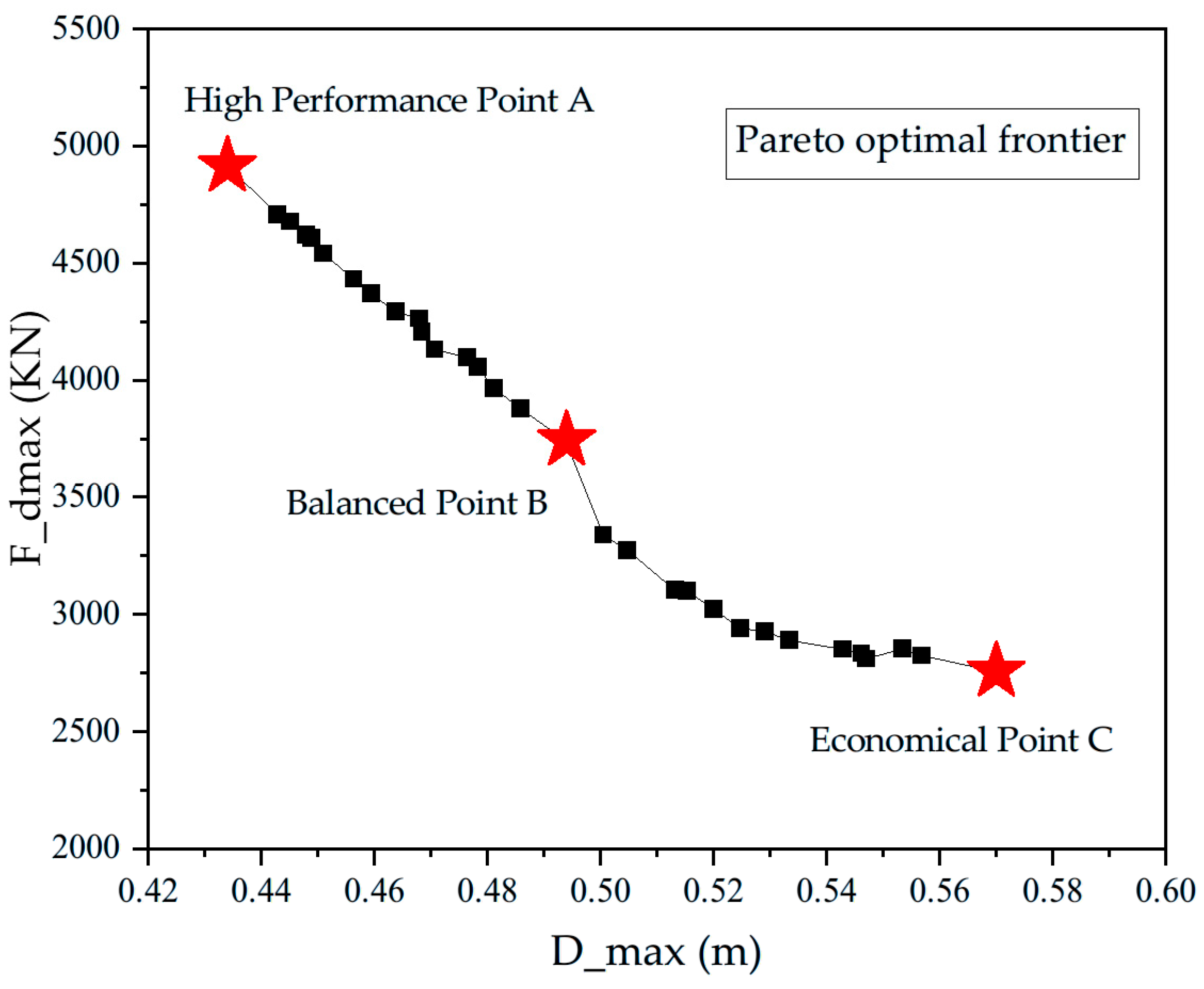
Figure A2.
Pareto optimal frontier for Bridge M3 obtained from the hybrid surrogate NSGA-II framework.
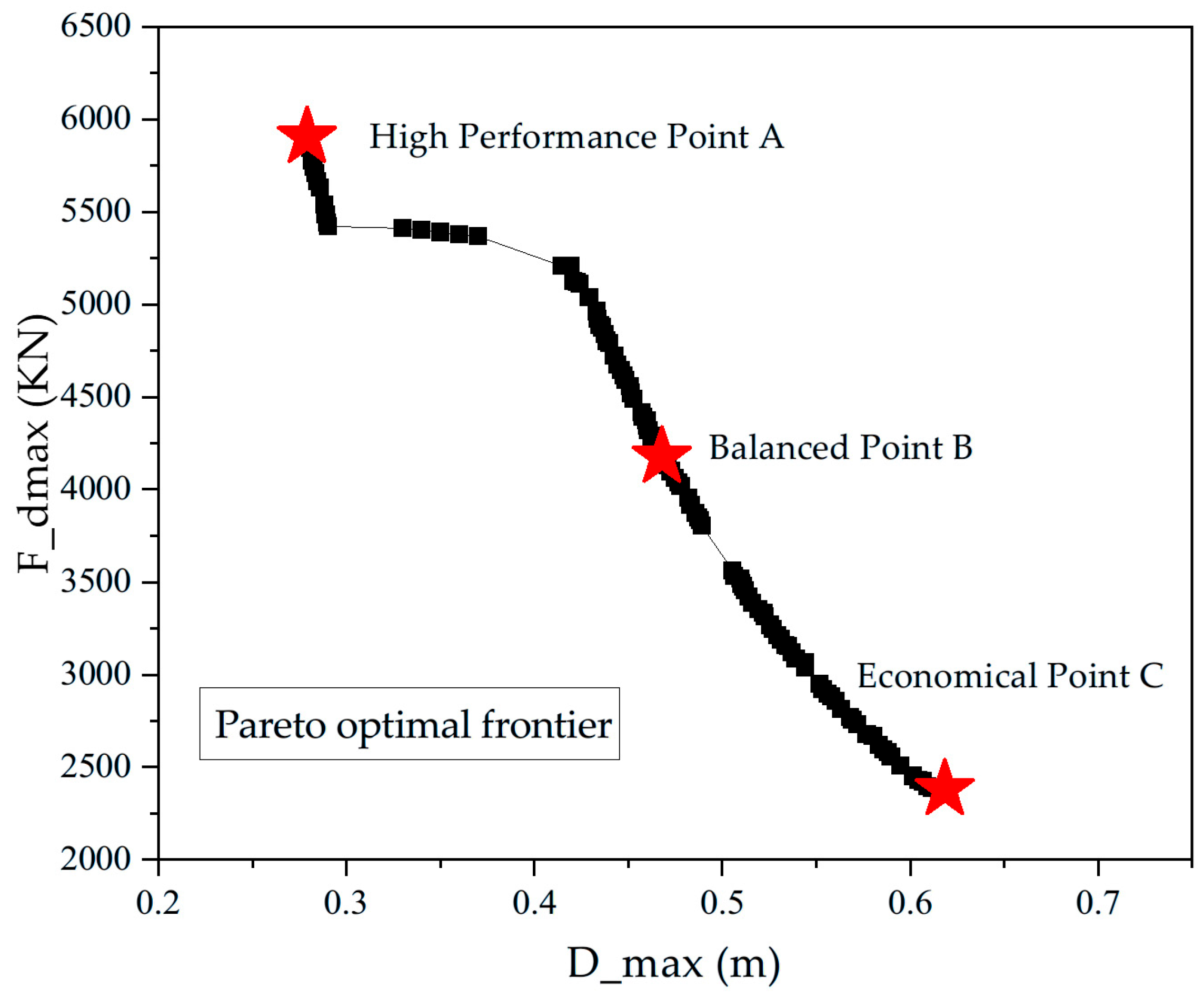
Appendix C
The uncertainty quantification, algorithm benchmarking, and robustness checks presented in Section 3.5 for Bridge M3 were also performed for Bridges M1 and M2. The results, summarized in Table A2, demonstrate consistent patterns: COV values below 0.25 for all EDPs, computational savings of approximately two orders of magnitude compared to conventional optimization, and stable Pareto frontiers under random ground motion subsets. These findings confirm that the conclusions drawn from the detailed M3 analysis are representative of the framework’s performance across the entire range of bridge configurations studied.
Table A2.
Summary of validation results for Bridges M1 and M2.
References
- Gimsing, N.J.; Georgakis, C.T. Cable Supported Bridges: Concept and Design, 3rd ed.; John Wiley & Sons: Hoboken, NJ, USA, 2012. [Google Scholar]
- Camara, A.; Efthymiou, E. Deck-tower interaction in the transverse seismic response of cable-stayed bridges and optimum configurations. Eng. Struct. 2016, 124, 494–506. [Google Scholar] [CrossRef] [Scilit]
- Fujino, Y.; Siringoringo, D.M. Vibration mechanisms and controls of long-span bridges: A review. Struct. Eng. Int. 2013, 23, 248–268. [Google Scholar] [CrossRef] [Scilit]
- Camara, A.; Astiz, M.A. Analysis and control of cable-stayed bridges subject to seismic action. Struct. Eng. Int. 2014, 24, 27–36. [Google Scholar] [CrossRef] [Scilit]
- Gao, L.; Liu, Z.; Dai, F.; Chen, J. Response analysis of a long-span cable-stayed bridge with ultra-high piles subjected to near-fault ground motions considering deep-water, sedimentation, local site, and wave-passage effect. Adv. Bridge Eng. 2024, 5, 34. [Google Scholar] [CrossRef] [Scilit]
- Soneji, B.B.; Jangid, R.S. Passive hybrid systems for earthquake protection of cable-stayed bridges. Eng. Struct. 2007, 29, 57–70. [Google Scholar] [CrossRef] [Scilit]
- Crespi, P.; Zucca, M.; Valente, M. On the collapse evaluation of existing RC bridges exposed to corrosion under horizontal loads. Eng. Fail. Anal. 2020, 116, 104727. [Google Scholar] [CrossRef] [Scilit]
- Symans, M.D.; Charney, F.A.; Whittaker, A.S.; Constantinou, M.C.; Kircher, C.A.; Johnson, M.W.; McNamara, R.J. Energy dissipation systems for seismic applications: Current practice and recent developments. J. Struct. Eng. 2008, 134, 3–21. [Google Scholar] [CrossRef] [Scilit]
- Li, H.; Li, L.; Hu, R.; Ye, M. Simplified design of nonlinear damper parameters and seismic responses for long-span cable-stayed bridges with nonlinear viscous dampers. Front. Struct. Civ. Eng. 2024, 18, 1103–1116. [Google Scholar] [CrossRef] [Scilit]
- Martínez-Rodrigo, M.D.; Filiatrault, A. A case study on the application of passive control and seismic isolation techniques to cable-stayed bridges: A comparative investigation through non-linear dynamic analyses. Eng. Struct. 2015, 99, 232–252. [Google Scholar] [CrossRef] [Scilit]
- Soares, R.W.; Barroso, L.R.; Al-Fahdawi, O.A.S. Response attenuation of cable-stayed bridge subjected to central US earthquakes using neuro-fuzzy and simple adaptive control. Eng. Struct. 2020, 203, 109874. [Google Scholar] [CrossRef] [Scilit]
- Iemura, H.; Pradono, M.H. Passive and semi-active seismic response control of a cable-stayed bridge. J. Struct. Control 2002, 9, 189–204. [Google Scholar] [CrossRef] [Scilit]
- Pan, P.; Yan, H.; Wang, T.; Xu, P.; Xie, Q. Development of steel dampers for bridges to allow large displacement through a vertical free mechanism. Earthq. Eng. Eng. Vib. 2014, 13, 375–388. [Google Scholar] [CrossRef] [Scilit]
- Marler, R.T.; Arora, J.S. Survey of multi-objective optimization methods for engineering. Struct. Multidiscip. Optim. 2004, 26, 369–395. [Google Scholar] [CrossRef] [Scilit]
- Puthanpurayil, A.M.; Lavan, O.; Dhakal, R.P. Multi-objective loss-based optimization of viscous dampers for seismic retrofitting of irregular structures. Soil Dyn. Earthq. Eng. 2020, 129, 105765. [Google Scholar] [CrossRef] [Scilit]
- Wen, J.; Han, Q.; Xie, Y.; Du, X.; Zhang, J. Performance-based seismic design and optimization of damper devices for cable-stayed bridge. Eng. Struct. 2021, 237, 112043. [Google Scholar] [CrossRef] [Scilit]
- Zhu, J.; Zhang, W.; Zheng, K.F.; Li, H.G. Seismic Design of a Long-Span Cable-Stayed Bridge with Fluid Viscous Dampers. Pract. Period. Struct. Des. Constr. 2016, 21, 04015006. [Google Scholar] [CrossRef] [Scilit]
- Deng, W.; Wang, H.; Li, A.; Liu, J. Parametric analysis on viscous dampers for earthquake mitigation of continuous bridges in high intensity region. J. Vib. Shock. 2012, 31, 92–97. (In Chinese) [Google Scholar] [CrossRef]
- Vader, T.S.; McDaniel, C.C. Influence of Dampers on Seismic Response of Cable Supported Bridge Towers. J. Bridge Eng. 2007, 12, 373–379. [Google Scholar] [CrossRef] [Scilit]
- Moustapha, M.; Sudret, B. Surrogate-assisted reliability-based design optimization: A survey and a unified modular framework. Struct. Multidiscip. Optim. 2019, 60, 2157–2176. [Google Scholar] [CrossRef] [Scilit]
- Ministry of Housing and Urban-Rural Development of the People’s Republic of China. Code for Seismic Design of Urban Bridges (CJJ 166-2011); China Architecture & Building Press: Beijing, China, 2011.
- Sun, H.; Burton, H.V.; Huang, H. Machine learning applications for building structural design and performance assessment: State-of-the-art review. J. Build. Eng. 2021, 33, 101816. [Google Scholar] [CrossRef] [Scilit]
- Mangalathu, S.; Heo, G.; Jeon, J.-S. Artificial neural network based multi-dimensional fragility development of skewed concrete bridge classes. Eng. Struct. 2018, 162, 166–176. [Google Scholar] [CrossRef] [Scilit]
- Wang, Z.; Shafieezadeh, A. REAK: Reliability analysis through error rate-based adaptive Kriging. Reliab. Eng. Syst. Saf. 2019, 182, 33–45. [Google Scholar] [CrossRef] [Scilit]
- Hu, Z.; Mahadevan, S. A single-loop kriging surrogate modeling for time-dependent reliability analysis. J. Mech. Des. 2016, 138, 061406. [Google Scholar] [CrossRef] [Scilit]
- Wang, J.; Shahani, N.M.; Zheng, X.; Jia, H.; Wei, X. Machine learning-based analyzing earthquake-induced slope displacement. PLoS ONE 2025, 20, e0314977. [Google Scholar] [CrossRef] [Scilit]
- Deb, K.; Pratap, A.; Agarwal, S.; Meyarivan, T. A fast and elitist multiobjective genetic algorithm: NSGA-II. IEEE Trans. Evol. Comput. 2002, 6, 182–197. [Google Scholar] [CrossRef] [Scilit]
- Zhou, A.; Qu, B.-Y.; Li, H.; Zhao, S.-Z.; Suganthan, P.N.; Zhang, Q. Multiobjective evolutionary algorithms: A survey of the state of the art. Swarm Evol. Comput. 2011, 1, 32–49. [Google Scholar] [CrossRef] [Scilit]
- Zhang, R.; An, L.; Yang, X.; He, L.; Huang, Z. A distributed inference method integrating causal analysis and surrogate models. Reliab. Eng. Syst. Saf. 2025, 257, 110863. [Google Scholar] [CrossRef] [Scilit]
- De Domenico, D.; Ricciardi, G. An enhanced base isolation system equipped with optimal tuned mass damper inerter (TMDI). Earthq. Eng. Struct. Dyn. 2018, 47, 1169–1192. [Google Scholar] [CrossRef] [Scilit]
- Hu, Y.; Guo, W.; Xu, Z.; Shi, C. Physics knowledge-based transfer learning between buildings for seismic response prediction. Soil. Dyn. Earthq. Eng. 2024, 177, 108420. [Google Scholar] [CrossRef] [Scilit]
- Pan, S.J.; Yang, Q. A survey on transfer learning. IEEE Trans. Knowl. Data Eng. 2010, 22, 1345–1359. [Google Scholar] [CrossRef] [Scilit]
- Azimi, M.; Eslamlou, A.D.; Pekcan, G. Data-driven structural health monitoring and damage detection through deep learning: State-of-the-art review. Sensors 2020, 20, 2778. [Google Scholar] [CrossRef] [Scilit]
- American Society of Civil Engineers (ASCE/SEI). Minimum Design Loads and Associated Criteria for Buildings and Other Structures (ASCE/SEI 7-22); American Society of Civil Engineers: Reston, VA, USA, 2022. [Google Scholar]
- ASCE Committee on Cable-Stayed Bridges. Guidelines for the Design of Cable-Stayed Bridges; American Society of Civil Engineers: New York, NY, USA, 1992. [Google Scholar]
- Wang, H.; Chen, C.; Xing, C.; Li, A. Influence of structural parameters on dynamic characteristics and wind-induced buffeting responses of a super-long-span cable-stayed bridge. Earthq. Eng. Eng. Vib. 2014, 13, 389–399. [Google Scholar] [CrossRef] [Scilit]
- CRRC Times New Material Technology Co., Ltd. Fluid Viscous Damping Devices [Product Catalog]. Available online: https://crrcgc.cc/sdxc/2022-03/05/article_0FF5FC7904954C52B0FADD92D02E2BE3.html (accessed on 1 October 2025).
- Pigouni, A.E.; Borella, R.; Infanti, S.; Castellano, M.G. Fluid Viscous Dampers for the 1915 Çanakkale Bridge in Turkey. In Proceedings of the World Conference on Seismic Isolation; Cimellaro, G.P., Ed.; Springer: Cham, Switzerland, 2023; pp. 478–487. [Google Scholar] [CrossRef] [Scilit]
- Singh, M.P.; Verma, N.P.; Moreschi, L.M. Seismic analysis and design with Maxwell dampers. J. Eng. Mech. 2003, 129, 273–282. [Google Scholar] [CrossRef] [Scilit]
- Yi, J.; Zhou, J.; Ye, X. Seismic control of cable-stayed bridge using negative stiffness device and fluid viscous damper under near-field ground motions. J. Earthq. Eng. 2022, 26, 2642–2659. [Google Scholar] [CrossRef] [Scilit]
- PEER Ground Motion Database. NGA-West2. Available online: https://ngawest2.berkeley.edu/ (accessed on 1 September 2025).
- Kwong, N.S.; Chopra, A.K.; McGuire, R.K. Evaluation of ground motion selection and modification procedures using a synthetic database. Earthq. Eng. Struct. Dyn. 2015, 44, 1841–1861. [Google Scholar] [CrossRef] [Scilit]
- Wu, C.; He, X.; He, L.; Zhao, X.; Wang, Y.; Li, C.; Yang, Y.; Zhang, X. Improving cable-stayed bridge longitudinal aseismic capability via fluid viscous damper parametric optimization and experimental investigation. Structures 2023, 57, 105199. [Google Scholar] [CrossRef] [Scilit]
- Li, G.; Hu, T.; Bai, D. BP neural network improved by sparrow search algorithm in predicting debonding strain of FRP-strengthened RC beams. Adv. Civ. Eng. 2021, 2021, 9979028. [Google Scholar] [CrossRef] [Scilit]
- Zhao, D.; Wang, H.; Yu, M. Optimization of cable tension in large-span cable-stayed bridges based on RBF neural network and improved sea-gull algorithm. Sci. Rep. 2025, 15, 42725. [Google Scholar] [CrossRef] [Scilit]
- Wu, Y.; Zhang, L.; Liu, H.; Lu, P. Stress prediction of bridges using ANSYS soft and general regression neural network. Structures 2022, 40, 812–823. [Google Scholar] [CrossRef] [Scilit]
- Xu, L.; Bi, K.; Gao, J.-F.; Xu, Y.; Zhang, C. Analysis on parameter optimization of dampers of long-span double-tower cable-stayed bridges. Struct. Infrastruct. Eng. 2020, 16, 1286–1301. [Google Scholar] [CrossRef] [Scilit]
- Rebello, C.M.; Costa, E.A.; Sánchez, A.S.; Vides, F.; Nogueira, I.B.R. Assuring optimality in surrogate-based optimization: A novel theorem and its practical implementation in pressure swing adsorption optimization. Can. J. Chem. Eng. 2025, 103, 1036–1059. [Google Scholar] [CrossRef] [Scilit]
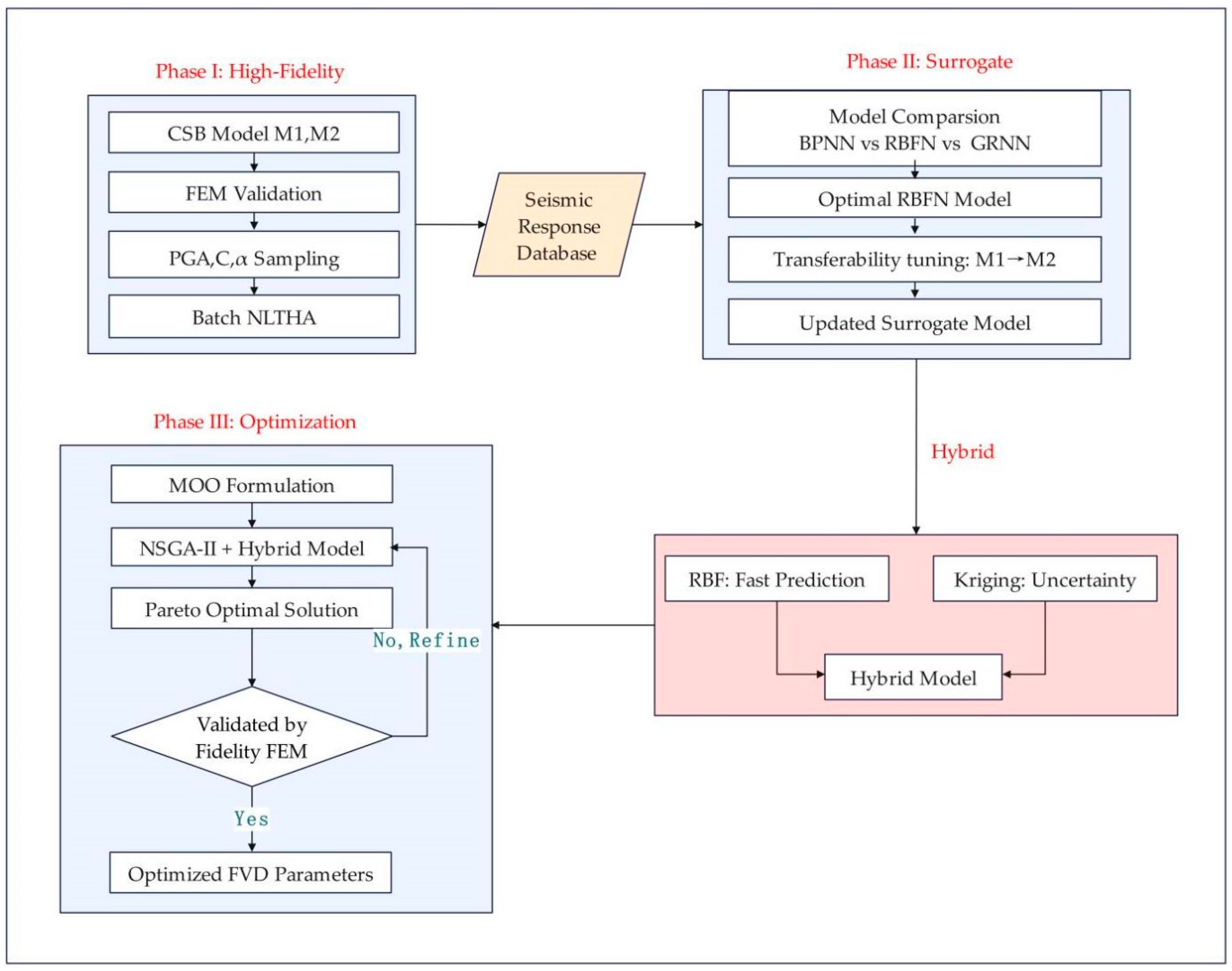
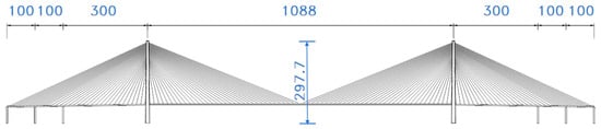
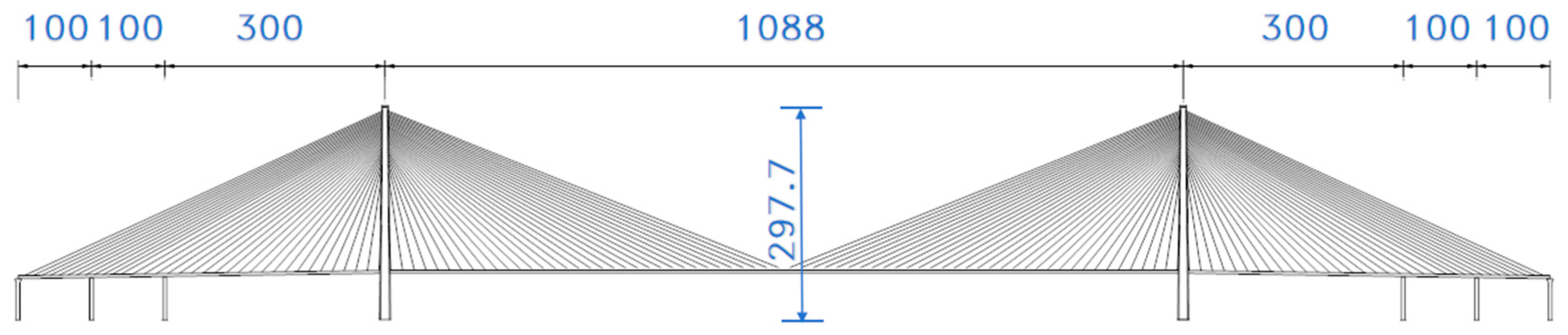


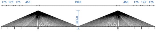
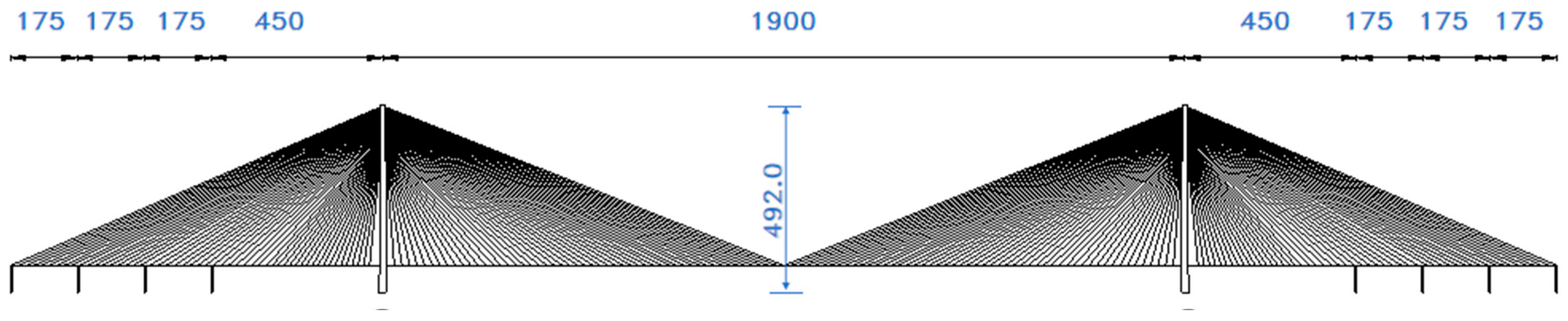
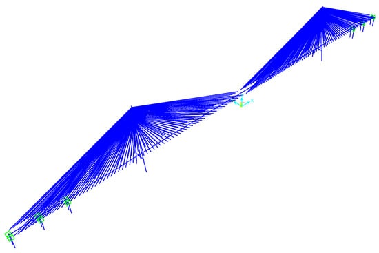
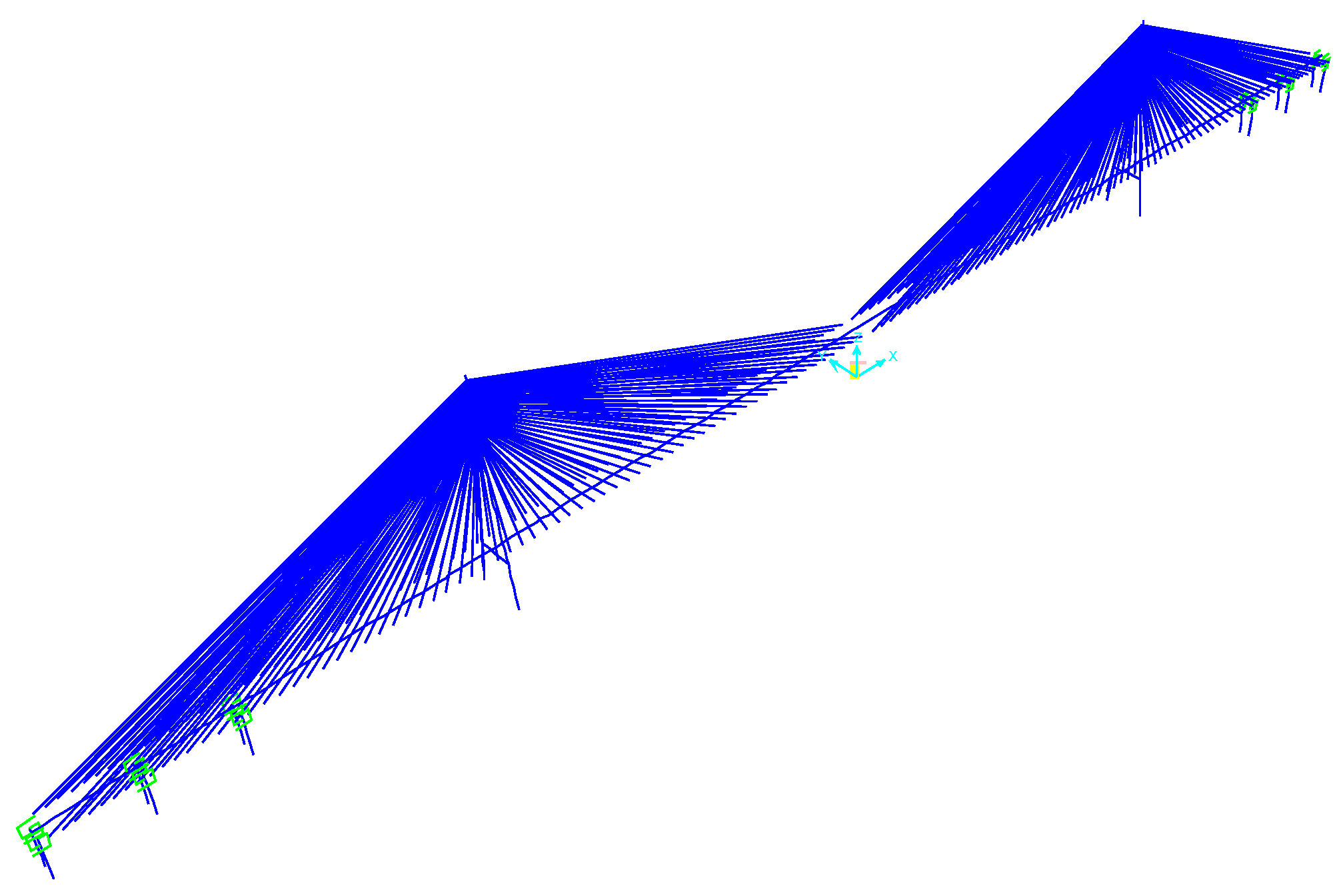
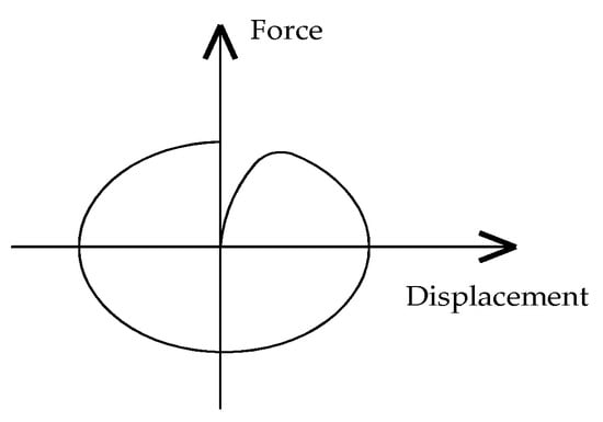
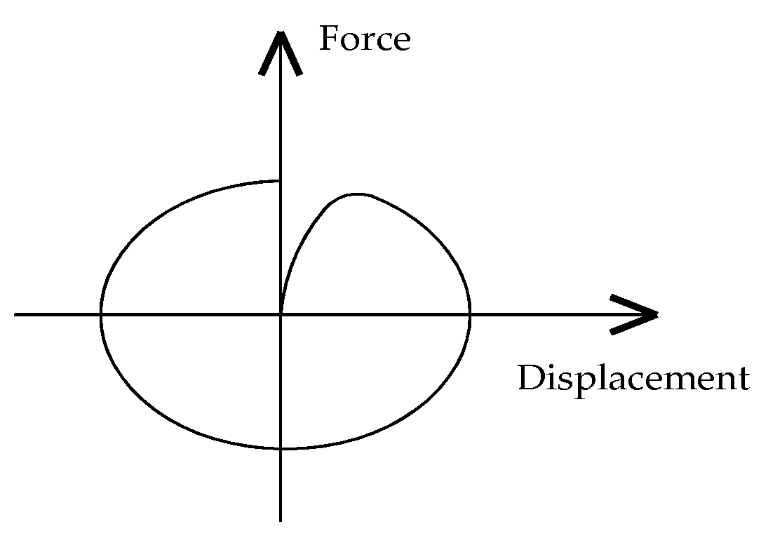
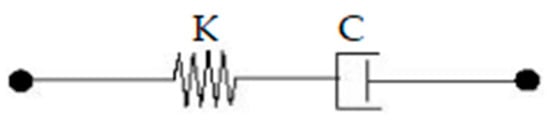
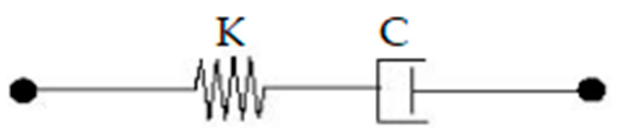
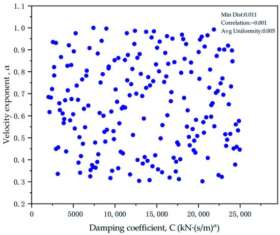
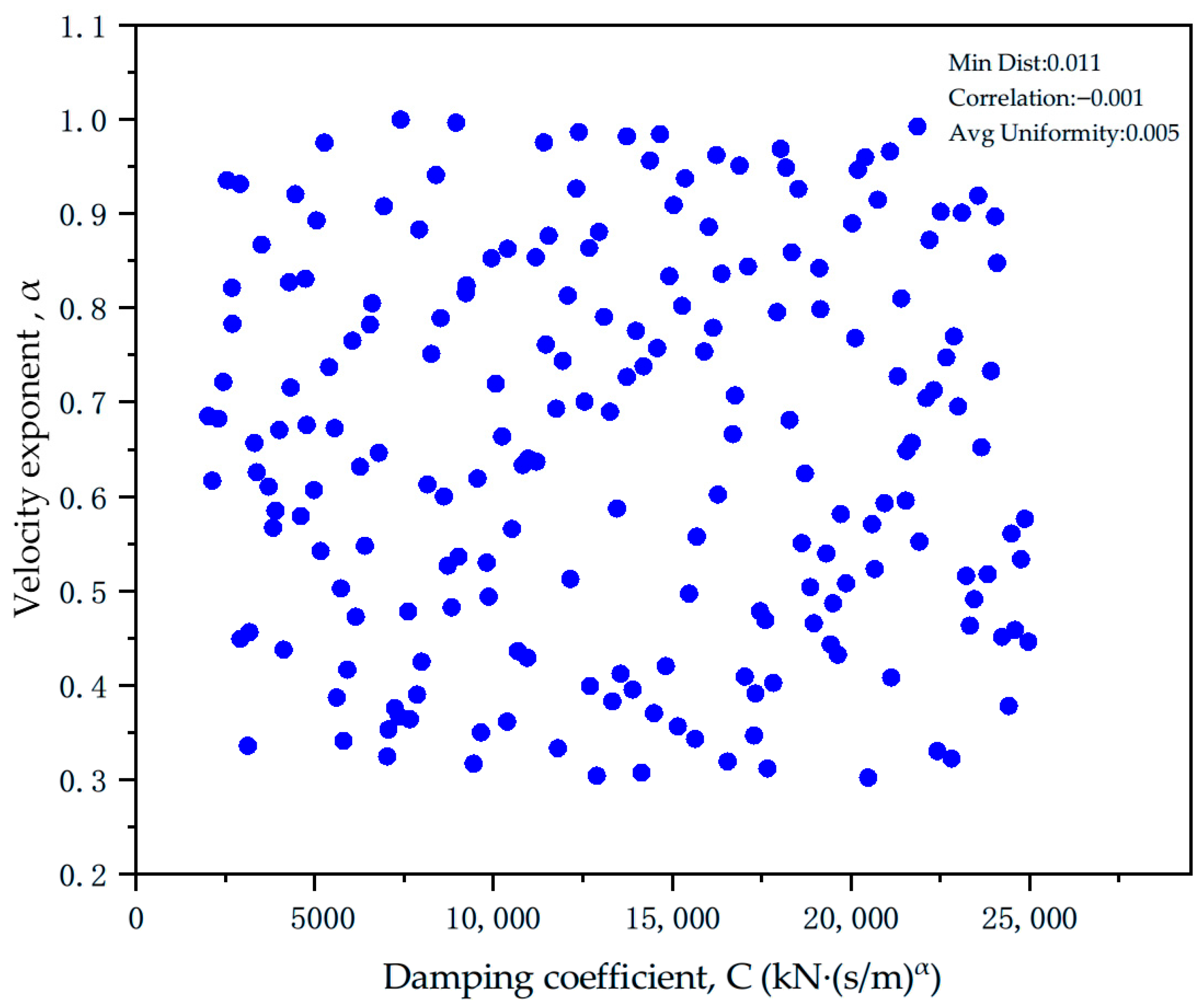
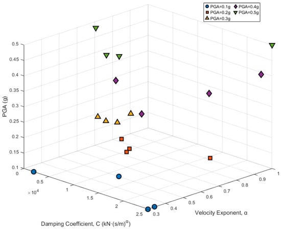
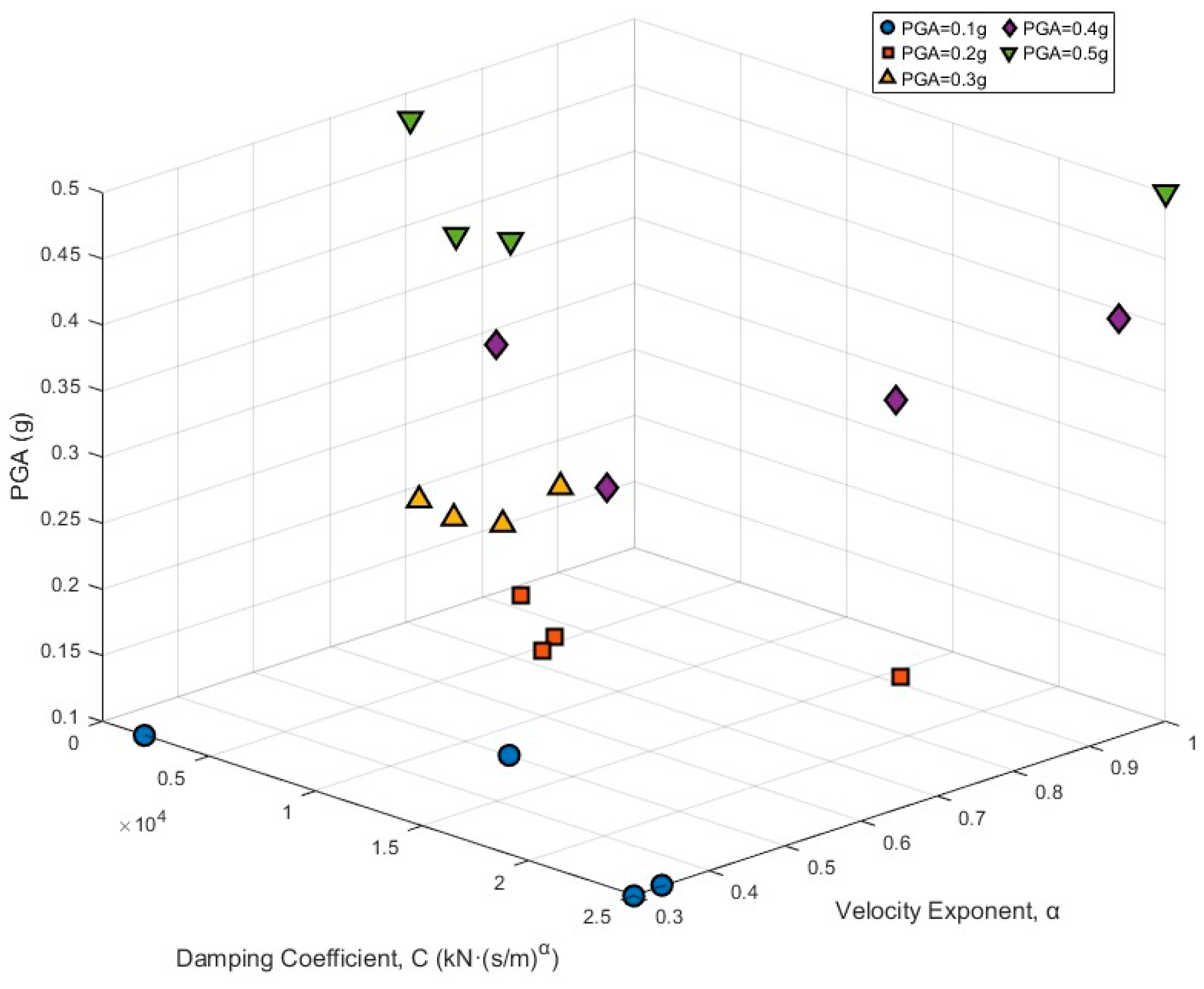
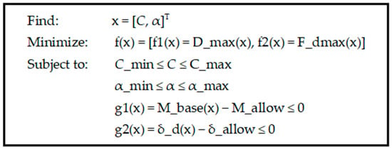
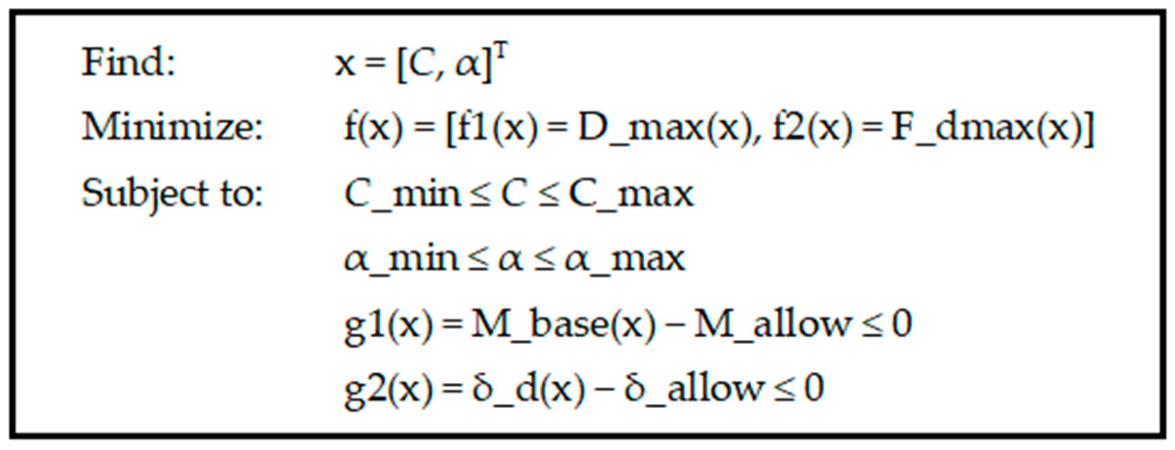
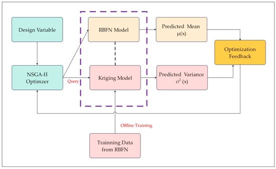
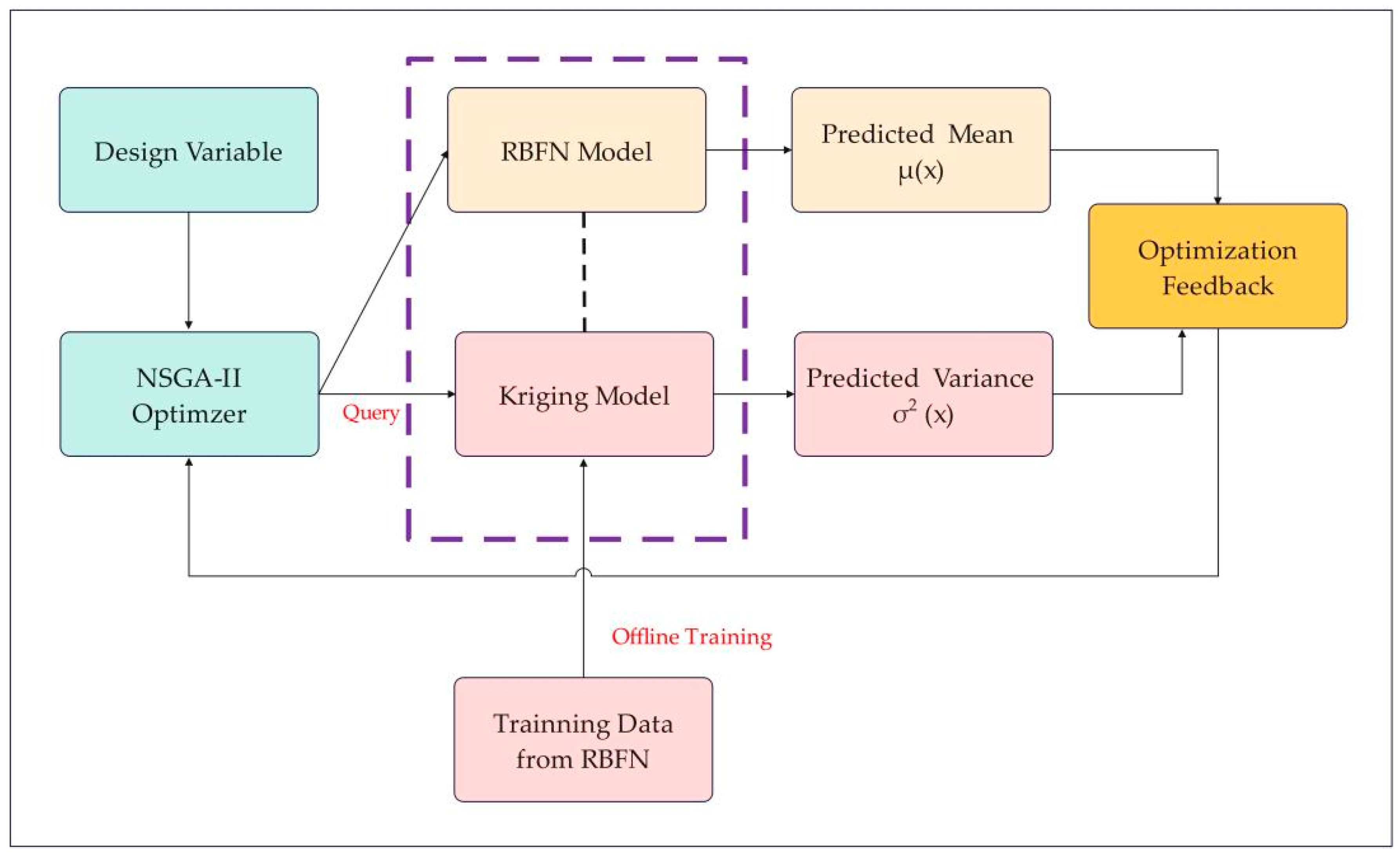
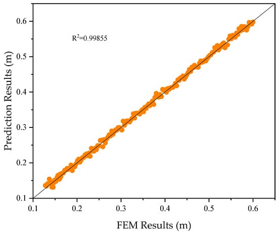
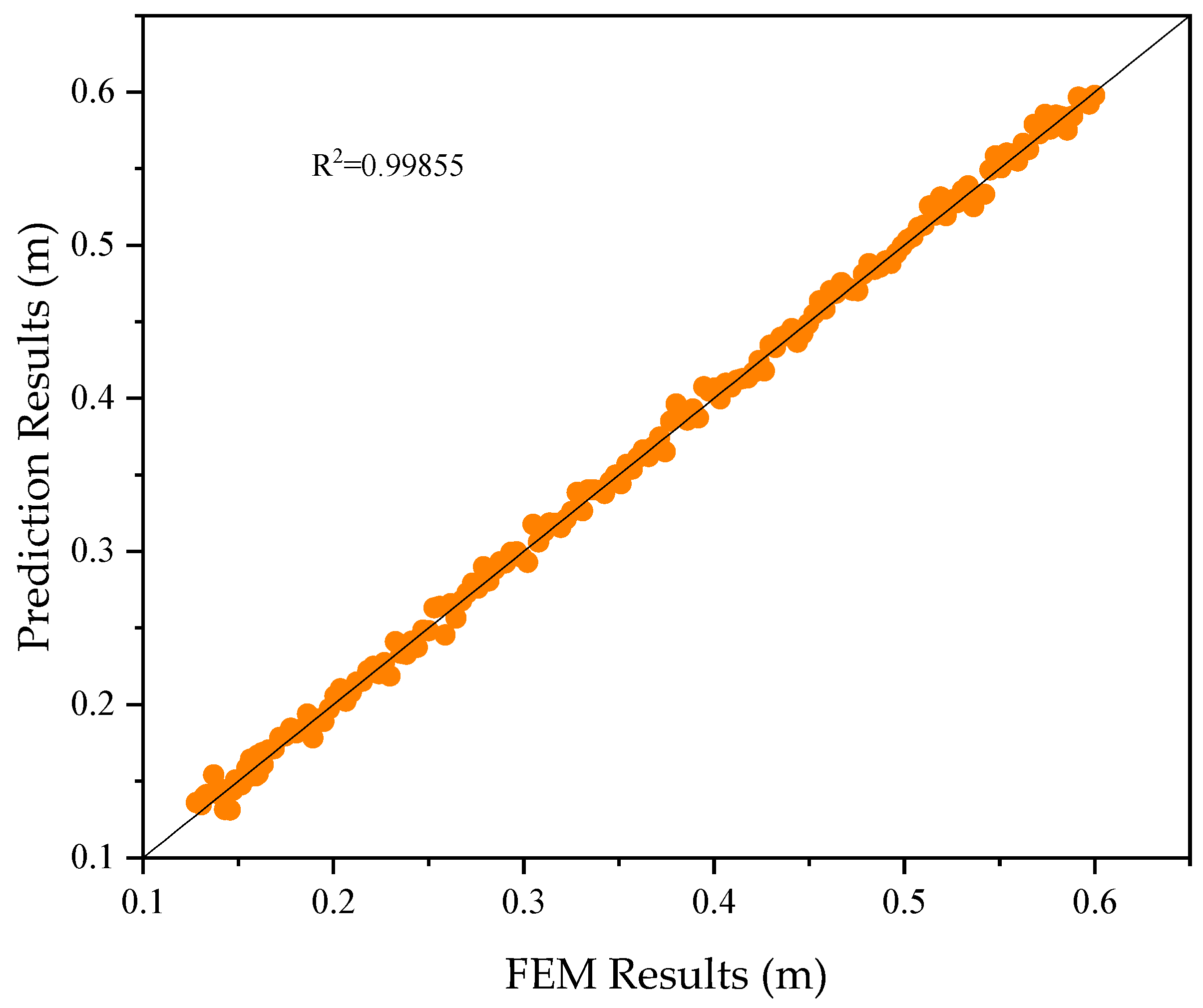
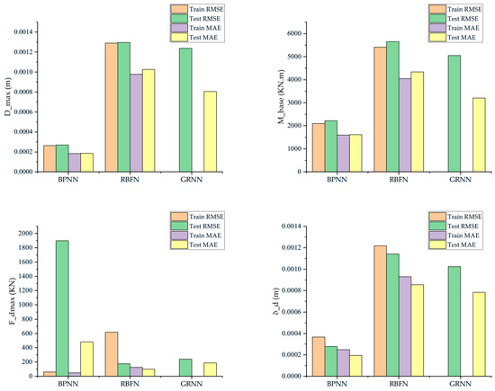
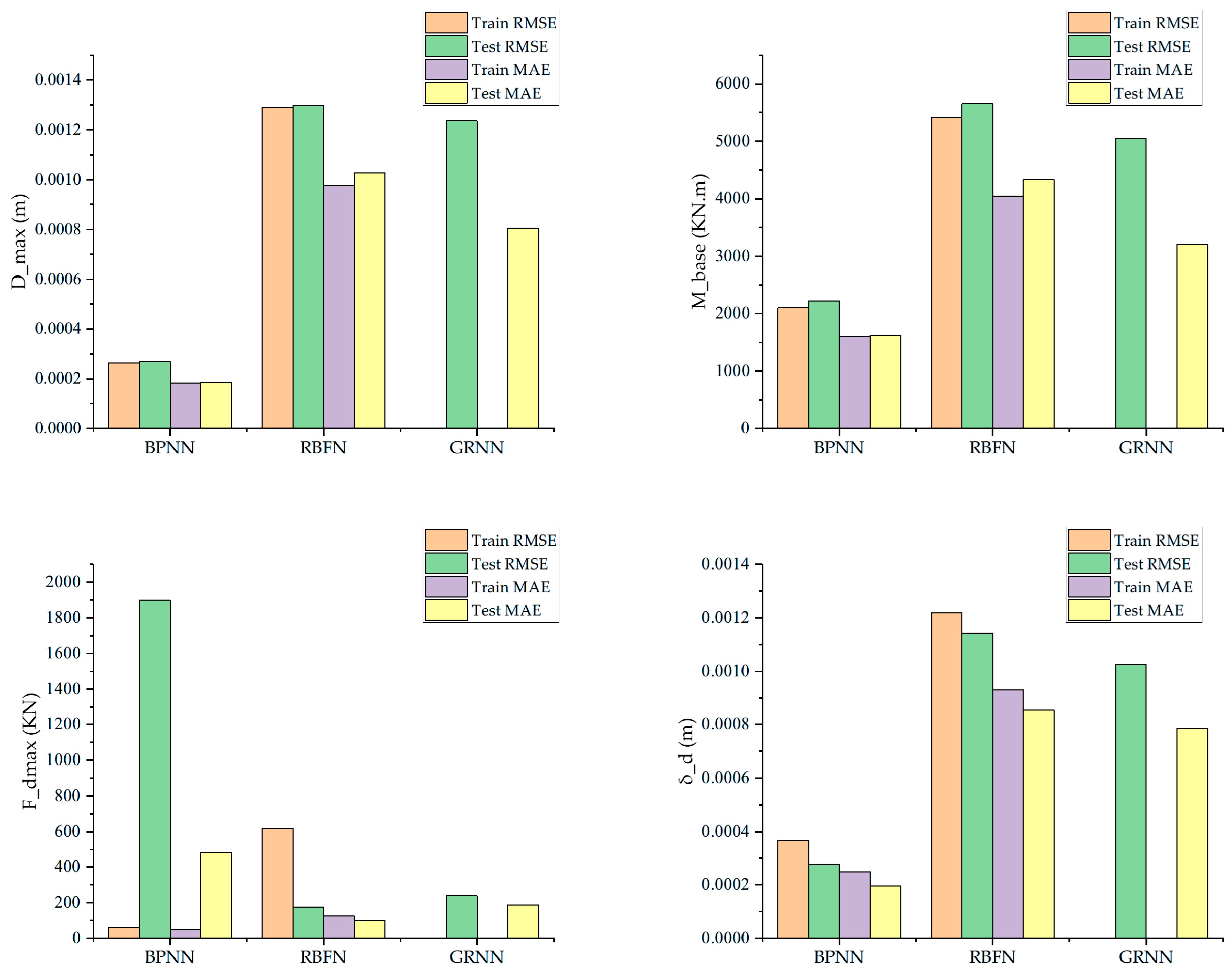
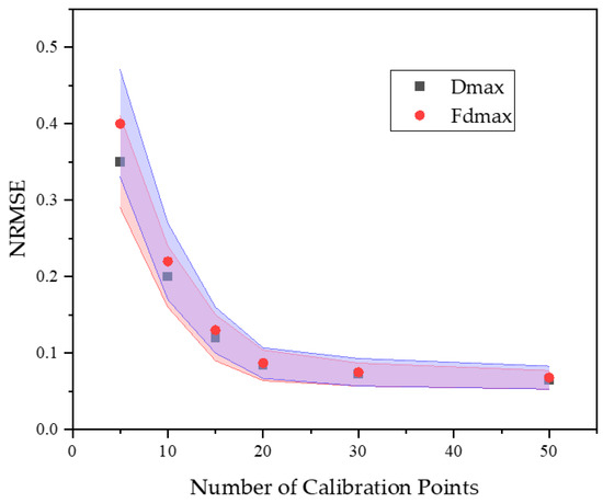
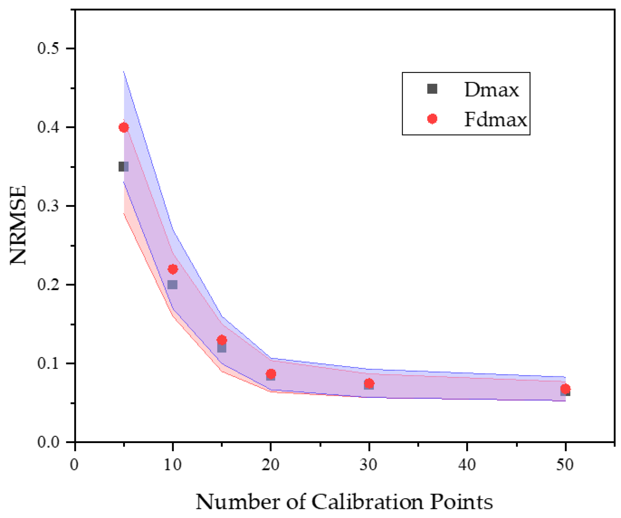
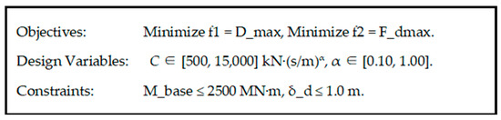
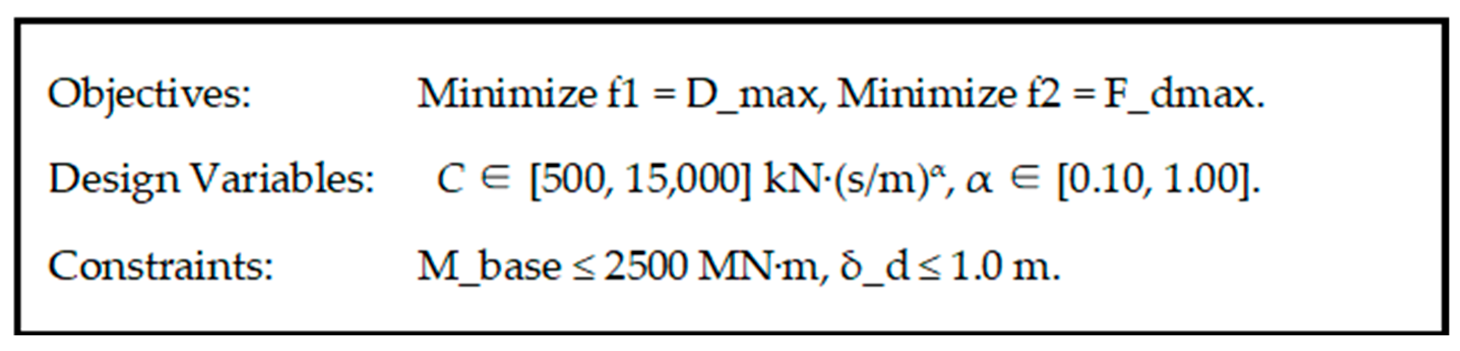
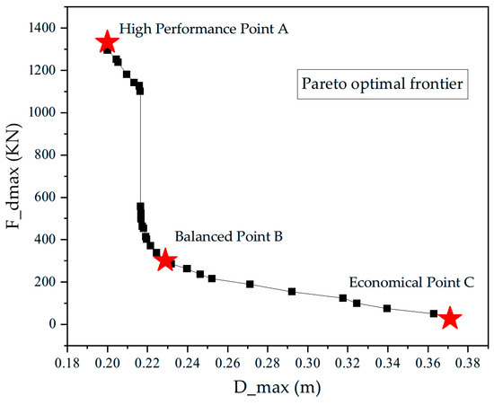
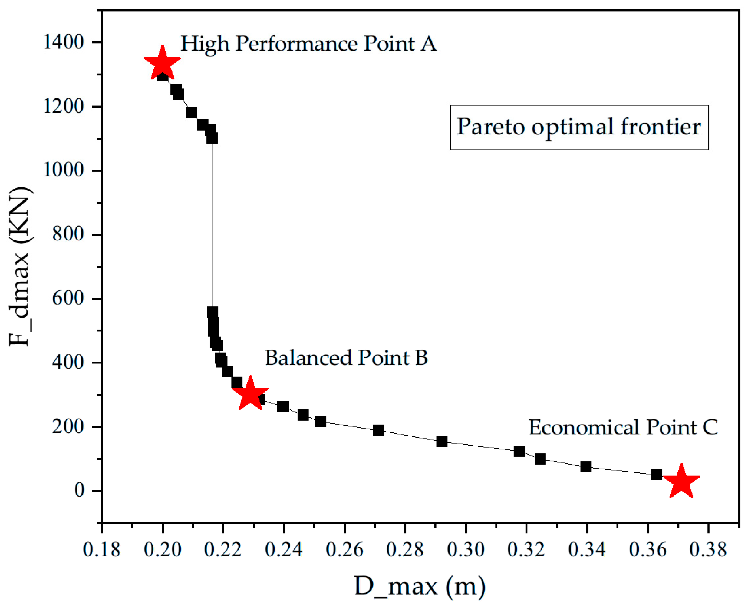

Disclaimer/Publisher’s Note: The statements, opinions and data contained in all publications are solely those of the individual author(s) and contributor(s) and not of MDPI and/or the editor(s). MDPI and/or the editor(s) disclaim responsibility for any injury to people or property resulting from any ideas, methods, instructions or products referred to in the content. |
© 2026 by the authors. Licensee MDPI, Basel, Switzerland. This article is an open access article distributed under the terms and conditions of the Creative Commons Attribution (CC BY) license.