


Abstract
Price volatility in steel reinforcement bars (rebar) plays a pivotal role in managing construction project costs, with precise forecasting being essential for maintaining corporate profitability and ensuring market stability. This research conducts a comprehensive evaluation of five prominent forecasting models—Autoregressive Integrated Moving Average (ARIMA), eXtreme Gradient Boosting (XGBoost), Prophet, Long Short-Term Memory (LSTM), and Transformer—specifically applied to steel rebar price prediction. The study emphasizes the influence of feature selection, defined as the number of historical price data points utilized for prediction, on the accuracy of these models. Furthermore, it develops a hybrid forecasting framework grounded in a residual complementarity mechanism aimed at improving long-term predictive performance. The results reveal that the ARIMA model delivers consistent and reliable short-term forecasts, particularly within a two-month horizon, whereas the Prophet model effectively captures long-term price trends but suffers from notable short-term bias. A two-stage hybrid model (referred to as Combination Model II), which integrates ARIMA and Prophet through residual inversion, demonstrates superior forecasting accuracy over a six-month period. This hybrid approach surpasses the standalone ARIMA model by more than 70% across key evaluation metrics—including Root Mean Square Error (RMSE), Mean Absolute Error (MAE), Mean Absolute Percentage Error (MAPE), Symmetric Mean Absolute Percentage Error (SMAPE), and Mean Absolute Scaled Error (MASE)—and exceeds the performance of the standalone Prophet model by over 90%. This integration effectively combines the high short-term precision of ARIMA with the long-term trend stability of Prophet. Within the domain of machine learning and deep learning models, XGBoost achieves optimal predictive accuracy when utilizing between one and four features. The predictive performance of LSTM does not exhibit a straightforward linear relationship with the number of features; however, certain feature combinations enable it to outperform other models. Transformer models maintain stable accuracy when employing feature sets ranging from one to five and twelve to seventeen, but display considerable variability in performance when the feature count lies between five and twelve. This investigation delineates the optimal parameter ranges and contextual applicability for each model. The proposed hybrid forecasting methodology, alongside a model transfer strategy encompassing data preprocessing adjustments, parameter optimization, and weight adaptation, offers practical applicability to other commodity markets such as cement and concrete. Consequently, this research provides a scientifically grounded framework to support procurement decision-making processes within construction enterprises.
Keywords:
rebar price forecast; combination of forecasting models; XGBoost; ARIMA; Prophet; LSTM; Transformers 1. Introduction
In the cost structure of engineering projects, material expenses represent the predominant portion of total project investment, with large- and medium-scale construction endeavors typically extending over multiple years. Variations in material prices significantly influence the profitability of construction firms (Abdul Nabi et al. [1]; Amini et al. [2]; Elfahham [3]; Kar and Jha [4]; Onayev et al. [5]; Sharma and Goyal [6]). Precise forecasting of material prices improves the accuracy of overall project cost estimations, thereby safeguarding the realization of expected profit margins (Du et al. [7]; Fischer [8]; Hwang et al. [9]; Isikdag et al. [10]). As a fundamental construction material, fluctuations in rebar prices have substantial implications for project cost management. Existing forecasting methodologies—including traditional statistical models as well as machine learning and deep learning techniques—face inherent challenges in balancing short-term and long-term predictive accuracy while adapting to the complex and dynamic market conditions characteristic of the steel reinforcement industry.
To address these industry challenges and methodological limitations, this study delineates clear primary and secondary objectives. The primary aim is to develop a high-precision hybrid model for forecasting rebar prices. By integrating the complementary strengths of various individual models, the proposed approach seeks to markedly improve the long-term forecasting accuracy of average rebar prices over a six-month horizon, thereby mitigating the deficiencies of single models in capturing extended price trends. The secondary objectives encompass three key aspects: (1) systematically comparing the predictive performance of five representative models—ARIMA, XGBoost, Prophet, LSTM, and Transformers—across different feature selection parameters (i.e., the number of historical price points utilized for forecasting) and temporal horizons, to elucidate their respective advantages and limitations in short-term versus long-term rebar price prediction and to establish clear criteria for model selection; (2) investigating the optimal parameter ranges, such as feature value intervals, for each individual model in the context of rebar price forecasting, thereby providing practical guidance for parameter tuning in analogous predictive models within the construction materials sector; and (3) validating the practical applicability of the constructed hybrid model for industry stakeholders, ensuring its direct utility in operational decision-making processes within construction firms, steel manufacturers, and distributors following minimal parameter adjustments.
Current approaches to steel rebar price forecasting exhibit notable shortcomings. Traditional statistical models, such as ARIMA, demonstrate robust short-term predictive capabilities but are limited in capturing long-term trends and nonlinear fluctuations. Conversely, models like LSTM and Transformers effectively model complex nonlinear relationships but lack a standardized optimal feature selection range, resulting in unstable predictions sensitive to the number of input features. Existing hybrid models predominantly rely on simple aggregation techniques, neglecting the complementary strengths of individual models in short-term versus long-term forecasting—for example, Prophet excels in modeling long-term trends but exhibits considerable short-term bias, whereas ARIMA achieves high short-term accuracy but struggles with long-term trend representation. The complementary residual error distributions observed between these models provide a solid foundation for developing novel hybrid models that address current deficiencies in fusion logic and coordination.
This research is highly pertinent to industrial practice, offering actionable solutions for all participants in the rebar supply chain. Construction enterprises can leverage the findings to formulate scientifically grounded procurement strategies, secure costs, and mitigate risks associated with price volatility. Similarly, steel manufacturers and distributors may optimize production scheduling and inventory management to achieve efficient resource allocation.
The five models selected for this investigation—ARIMA, XGBoost, Prophet, LSTM, and Transformers—represent the three principal methodological categories: traditional statistical methods, machine learning, and deep learning, each characterized by distinct attributes. ARIMA, a classical statistical model, provides strong interpretability for short-term forecasting and serves as a benchmark. XGBoost excels in nonlinear fitting and noise robustness, delivering high efficiency in engineering predictions. Prophet effectively handles missing and anomalous data, adapting well to long-term trend capture. LSTM addresses the gradient vanishing problem inherent in recurrent neural networks, excelling at modeling medium- to long-term dependencies. Transformers utilize self-attention mechanisms to enable parallel computation and capture multi-scale dependencies. Conducting a multi-model comparison facilitates a comprehensive evaluation of diverse methodologies, mitigating bias and establishing a foundation for hybrid model construction.
The forecasting methodology developed herein is transferable to analogous commodity markets, such as cement and non-ferrous metals. This transferability involves three stages: first, adjusting data preprocessing techniques to accommodate the specific characteristics of the target market data and ensure continuity; second, optimizing model parameters in accordance with the price fluctuation patterns of the target market; and third, validating the hybrid model’s adaptability and adjusting the weighting of individual models to align with the pricing mechanisms of the target market.
The innovations of this research are threefold. First, it proposes a two-stage residual complementary hybrid model that initially integrates ARIMA and Prophet to enhance long-term forecasting accuracy, subsequently incorporating ARIMA’s short-term strengths to achieve balanced performance across temporal horizons. Second, it systematically investigates the optimal feature value ranges for models such as XGBoost and LSTM, addressing a gap in parameter selection guidance for similar models. Third, it elucidates the complementary mechanism between ARIMA and Prophet through residual distribution analysis, offering novel insights for the development of residual-complementary hybrid models. Unlike most studies that focus primarily on result presentation and simple parameter optimization, this research adopts a data input perspective to clarify the relationship between feature selection and model performance, thereby deepening the analytical rigor.
The structure of this paper is as follows: Section 2 reviews the current state of rebar price forecasting research, analyzing the strengths and weaknesses of the three model categories; Section 3 details the construction processes of the five models; Section 4 compares the predictive results of individual models to identify effective candidates; Section 5 develops and optimizes the two-stage hybrid model; finally, conclusions are drawn, limitations are discussed, and directions for future research are proposed.
For clarity, models employing varying numbers of feature values—that is, the quantity of historical price data points used for prediction—are uniformly denoted using the format “Model Name + Number” (e.g., “XGBoost1” indicates an XGBoost model utilizing one feature value, whereas “LSTM5” denotes an LSTM model employing five feature values).
2. Research Background
Accurately forecasting rebar prices is essential for effective cost management in construction projects and the procurement of structural steel. Due to the temporal dynamics and inherent volatility of rebar pricing, existing research has predominantly concentrated on time series analytical approaches. In recent years, a range of statistical and machine learning methodologies have been extensively employed to predict prices of rebar and steel. Nevertheless, the performance of these models exhibits considerable variability across diverse contexts, and there is a notable absence of comprehensive and systematic comparative evaluations.
2.1. Statistical Models
Conventional statistical models predominantly utilize mathematical frameworks to identify linear patterns within time series data; however, their effectiveness in capturing intricate market dynamics remains limited. Kapl and Müller [11] conducted a comparative analysis of the AMNIA and Multivariate Singular Spectrum Analysis (MSSA) models in forecasting prices of US hot-rolled coil steel. Their findings indicated that the predictive accuracy of the MSSA model improved as the length of the time series increased. Nonetheless, both models exhibited difficulties in accurately modeling abrupt short-term fluctuations, such as sudden spikes in raw material costs. More recent research efforts have sought to enhance statistical forecasting approaches. For instance, Faghih and Kashani [12] developed a Vector Error Correction (VEC) model to predict US construction steel prices, incorporating macroeconomic variables to achieve robust performance in both short- and long-term forecasts. Despite these strengths, the model’s dependence on stable economic conditions constrains its applicability in the context of increased market volatility following the pandemic. Similarly, Uvarova et al. [13] integrated ARIMA models with expert elicitation to forecast rebar prices in two Russian regions, employing qualitative insights to mitigate the limitations inherent in purely statistical methods; however, this approach may be susceptible to subjective biases introduced by expert judgment. Additionally, Shiha and El-Adaway [14] identified Mexico’s Producer Price Index as a reliable leading indicator for steel prices and demonstrated that their optimized Vector Error Correction Model surpassed traditional models over an 18-month forecasting horizon, particularly in anticipatory predictions. Nevertheless, this model showed limited responsiveness to regional trade policy changes.
2.2. Machine Learning and Deep Learning Models
Machine learning models demonstrate considerable proficiency in capturing nonlinear relationships; however, their effectiveness is highly contingent upon data quality and parameter optimization, with findings differing across various studies. Marzouk et al. [15] analyzed Egyptian market data spanning 2000 to 2010, integrating fuzzy logic with neural networks to identify construction materials sensitive to price changes and to predict price fluctuations. This methodology aids contractors in tender bidding and procurement planning, while also enabling project owners to estimate total costs. Jiang et al. [16] emphasized the critical importance of reliable construction price forecasting for the industry, noting that price volatility influences multiple decision-making processes. They observed that prior research rarely accounts for global economic events and seasonal price variations; thus, their study incorporated these factors as dummy variables alongside macroeconomic indicators to develop a Vector Error Correction (VEC) model. This model outperformed traditional approaches and facilitated analysis of the effects of specific events on the industry.
Tang et al. [17] addressed uncertainty in building material price fluctuations by proposing an Improved Particle Swarm Optimization-Least Squares Support Vector Machine (IPSO-LSSVM) forecasting method. By enhancing the particle swarm algorithm to optimize Least Squares Support Vector Machine (LSSVM) parameters, this approach mitigates the local optimum problem inherent in standard Particle Swarm Optimization (PSO). Validation conducted in MATLAB revealed an average relative error of 2.11%, demonstrating superior accuracy and convergence relative to conventional algorithms, thereby confirming its practical applicability. Mi et al. [18] developed a Variational Mode Decomposition-Ensemble Empirical Mode Decomposition-Long Short-Term Memory (VMD-EEMD-LSTM) model for forecasting rebar futures prices, improving feature extraction through time series decomposition. This model surpassed single-model approaches in 14-day short-term forecasting but entails high computational demands, limiting its feasibility for enterprises with constrained technical resources.
Tian and Shang [19] proposed a hybrid Convolutional Neural Network-Long Short-Term Memory (CNN-LSTM) model to forecast HRB400 rebar prices. This model combines the spatial feature extraction capabilities of Convolutional Neural Networks (CNN) with the temporal dependency modeling of Long Short-Term Memory (LSTM) networks. The forecasting results exhibited significantly closer alignment with actual price fluctuations compared to single-model methods. However, the approach requires large-scale, high-frequency data, restricting its applicability in regions with incomplete datasets. Alcalde [20] utilized Nonlinear AutoRegressive (NAR), Nonlinear Input–Output (NIO), and Nonlinear AutoRegressive with eXogenous inputs (NARX) neural networks to predict Spanish hot-rolled coil prices, finding that the NARX model performed best due to its incorporation of external variables. Nonetheless, its predictive accuracy diminished during periods characterized by abrupt fluctuations in external factors such as energy prices.
Assaf et al. [21] employed a Deep Autoregressive Model (DeepAR)-based autoregressive recurrent network to forecast U.S. construction steel prices amid post-pandemic uncertainty, achieving an average absolute percentage error of only 4%. However, this probabilistic forecasting framework lacks sufficient interpretability for practical decision-making. Lederer et al. [22] observed that the sharp increase in construction costs during 2020–2021 complicated contractors’ ability to honor fixed contract prices, necessitating the use of price indices to forecast and reserve adjustment margins for risk mitigation. They applied four methodologies—including regression analysis and exponential smoothing—and identified the optimal approach through multi-criteria decision-making validated with statistical data, aiming to determine suitable forecasting methods for construction materials and engineering costs in Central and Eastern Europe.
Guo et al. [23] highlighted the critical role of accurate construction material price forecasting for project cost control and risk management, noting that strong nonlinearity and volatility undermine the effectiveness of traditional methods. They proposed the Complete Ensemble Empirical Mode Decomposition with Adaptive Noise-Variational Mode Decomposition-Gated Recurrent Unit-Autoregressive Integrated Moving Average (CEEMDAN-VMD-GRU-ARIMA) model, which optimizes Variational Mode Decomposition (VMD) parameters and adaptively selects prediction models, achieving an adjusted R2 of 81.10%. This model offers novel insights for short-term forecasting of construction materials. Ning et al. [24] developed a rebar price prediction model combining sliding windows with Categorical Boosting (CatBoost), demonstrating superior accuracy relative to multiple comparison models and robust fitting performance during the pandemic, thereby supporting decision-making for relevant stakeholders.
Merika et al. [25] constructed a machine learning decision support framework to evaluate trade-offs between continuing vessel operations and salvaging residual steel value. They compared the predictive performance of Long Short-Term Memory (LSTM) and Autoregressive Integrated Moving Average (ARIMA) models against traditional approaches for dry bulk freight rates and scrap steel prices, segmenting estimates by vessel type and incorporating macroeconomic variables to enhance robustness. This framework provides shipowners with a scalable tool for optimizing scrapping strategies. Xiong et al. [26] proposed a VMD-Sparrow Search Algorithm-LSTM (VMD-SSA-LSTM) hybrid model to improve construction material price forecasting accuracy. This method decomposes historical data using Variational Mode Decomposition (VMD), optimizes LSTM parameters via the Sparrow Search Algorithm (SSA), and aggregates predictions through LSTM modeling. Validation using Hengyang rebar price data demonstrated superior accuracy compared to Backpropagation (BP) neural networks, offering a practical tool for engineering cost management, budget planning, and risk mitigation.
2.3. Combined Model
Ensemble models leverage the advantages of multiple individual models; however, current studies predominantly utilize rudimentary aggregation techniques that lack sophisticated fusion strategies. Liu et al. [27] highlighted the construction sector’s pronounced vulnerability to fluctuations in material prices, noting that conventional econometric approaches are insufficient to effectively capture the sector’s frequent volatility. This review critically evaluates the deployment of data-driven methodologies, with an emphasis on machine learning, in forecasting construction material prices. It categorizes these approaches into causal modeling and time series analysis, advocating for the adoption of hybrid models to enhance project decision-making and cost control. Dai et al. [28] applied a residual inversion technique to integrate ARIMA and GM(1,1) models for predicting rebar prices in Guangzhou, demonstrating improved accuracy relative to individual models. Nonetheless, their fusion framework did not adequately exploit the complementary strengths of these models in addressing short-term versus long-term forecasting horizons. Zhang [29] refined the time series decomposition process by implementing an inverse variance-weighted fusion of multiplicative and additive models for rebar price prediction; however, the model’s performance exhibited sensitivity to the chosen decomposition methods and lacked robustness across different regions. Xu and Zhang [30,31,32] conducted comprehensive investigations into Chinese steel price forecasting by developing Gaussian process regression models for ten steel product categories, employing regional nonlinear neural networks for market analysis, and utilizing nonlinear autoregressive neural networks to predict scrap steel prices. While these models achieved high forecasting precision, their design was tailored specifically to the Chinese market context, neglecting international factors such as European carbon policy constraints, thereby limiting their generalizability. This analysis underscores the necessity for a thorough evaluation of the strengths and limitations inherent in existing modeling approaches.
2.4. Advantages and Limitations of the Three Categories of Models
2.4.1. Advantages
Statistical models are characterized by their straightforward structure, low computational demands, and high interpretability. Models such as ARIMA and VEC demonstrate strong performance in stable market conditions and are particularly well-suited for short-term forecasting involving linear trends. In contrast, machine learning and deep learning models exhibit a superior capacity to capture nonlinear relationships and complex features. Architectures including LSTM, CNN-LSTM, and Transformers effectively extract latent patterns from high-dimensional datasets, yielding enhanced predictive accuracy in volatile market environments. Hybrid models combine the complementary strengths of these approaches, integrating the linear trend-capturing ability of statistical models with the nonlinear feature extraction capabilities of machine learning techniques to improve forecasting robustness.
2.4.2. Limitations
Statistical models exhibit limited adaptability to nonlinear volatility and abrupt market shocks, often relying heavily on the assumption of data stationarity. They also face challenges in incorporating complex external factors such as geopolitical events or environmental policies. Machine learning and deep learning models, while powerful, require extensive data and computational resources, are prone to overfitting, and generally lack interpretability. Moreover, parameter tuning in these models lacks standardized procedures, and their performance tends to deteriorate in scenarios with limited sample sizes. Combination models frequently utilize simplistic weighting schemes without rigorous analysis of the underlying complementary mechanisms, resulting in fusion strategies that lack a solid theoretical foundation.
Current research in this domain is hindered by two primary deficiencies. First, there is an insufficient focus on market-specific characteristics. Although existing studies have developed various forecasting models based on national or regional datasets, these efforts remain inadequate given the substantial heterogeneity across global markets—for example, China’s policy-driven market, the market-oriented United States, and Europe’s carbon neutrality-constrained market—each of which demands tailored analytical approaches. Second, the depth of model analysis is often lacking; most studies prioritize the presentation of forecasting outcomes without thoroughly investigating the fundamental factors driving differences in model performance, such as the impact of feature selection mechanisms on the stability of models like XGBoost compared to Transformers.
This study seeks to address these gaps through the following strategies: (1) the selection of five representative models encompassing statistical, machine learning, and deep learning paradigms (ARIMA, XGBoost, Prophet, LSTM, and Transformers) to systematically compare their performance across varying feature sets and forecasting horizons, thereby providing a foundation for informed model selection in rebar price prediction; and (2) the development of a two-stage composite model based on rebar price data from Guangdong Province—the largest rebar consumption region in China—that exploits residual complementarity. This composite model integrates ARIMA’s proficiency in short-term forecasting with Prophet’s capability to capture long-term trends, offering methodological support for enhanced price forecasting accuracy.
3. Prediction Model Construction
This article selects five representative price prediction methods to establish a price prediction model, and the details of these methods will be discussed in the following sections.
3.1. Data Collection, Cleaning, and Analysis
3.1.1. Data Collection and Cleaning
The price data for threaded steel utilized in this study were sourced from the “Guangdong Province Construction Engineering Material Price Monitoring System” (http://cbprov.gldjc.com/gd/homepage) The website was accessed on 1 July 2024 to retrieve the complete price dataset spanning from 1 May 2018 to 31 December 2023. The selection of this platform as the primary data source was guided by three principal considerations:
- Authority and Reliability: This monitoring system is developed and managed under the auspices of relevant provincial authorities in Guangdong. The data are directly obtained from leading steel manufacturers, building material distributors, and procurement records associated with major construction projects within the province. The dataset undergoes rigorous multi-level verification and validation procedures, effectively mitigating subjective biases commonly present in self-reported corporate data. Consequently, this system is recognized as the official and authoritative repository for construction material price monitoring within Guangdong.
- Data Relevance and Completeness: The system specifically tracks prices of materials frequently employed in construction, including daily quotations for standard specifications of rebar such as HRB400E. This focus aligns closely with the research objective of forecasting rebar prices for construction applications. Moreover, the system has been operational continuously since 1 May 2018, thereby providing an uninterrupted and comprehensive time series of price data adequate for model training purposes.
- Regional Representativeness: Guangdong, as a leading economic province and infrastructure hub in China, ranks among the top regions nationally in terms of rebar consumption and circulation volume. Its market pricing reflects both national supply–demand dynamics and policy influences while also capturing regional market factors such as port-imported iron ore availability and local infrastructure investment cycles. Thus, data from Guangdong serve as a highly representative indicator of the broader national rebar market. Predictive insights derived from this regional dataset can be reasonably extrapolated to other economically advanced regions or applied in nationwide market analyses.
Given the variability of rebar prices across different steel mills and cities, attributable to the diversity of rebar materials used in construction, it is noteworthy that price differentials and trends among various rebar types and across cities exhibit consistent patterns. Accordingly, the price of HRB400E ɸ 25 rebar in Guangzhou was selected as a representative benchmark for data acquisition and organization. The monitoring website commenced operation on 1 May 2018; thus, price data for HRB400E ɸ 25 rebar spanning from 1 May 2018 to 31 December 2023 were collected as the foundational dataset.
To ensure data sufficiency for predictive model development, missing values were interpolated due to the release of threaded steel price information exclusively on working days, with no disclosures on weekends or national holidays. The interpolation employed was the arithmetic sequence method within linear interpolation, chosen for its ability to preserve data trend continuity while minimizing fluctuations.
In practical construction project management, forecasts of future prices primarily inform the preparation of material procurement plans on monthly, quarterly, and semiannual bases. Accordingly, the threaded steel price data were segmented into three intervals per month: early, mid, and late periods. Following segmentation, the triple standard deviation method was applied to identify and remove outliers, after which the mean price was calculated. This processed data facilitated the generation of the price trend chart for HRB400E ɸ 25 rebar in Guangzhou from 1 May 2018 to 31 December 2023, as depicted in Figure 1.
Figure 1.
Price trend chart of HRB400E ɸ 25 rebar in Guangzhou from 1 May 2018 to 31 December 2023.
3.1.2. Data Analysis
To scientifically select the most suitable model, a quantitative analysis was conducted across three core dimensions: trend characteristics, seasonal patterns, and dataset scale. The results are as follows:
Trend Analysis
Employing dual validation through linear trend fitting and the Mann–Kendall trend test:
- (1)
- Linear Trend Fitting:
The price sequence fitting equation is as follows:
( denotes the time sequence number and denotes the price).
The negative slope indicates that rebar prices exhibited a weak downward trend from 2018 to 2023.
- (2)
- Mann–Kendall Test
The statistical measure Z = −1.87 (p-value = 0.062 > 0.05) indicates that the trend is not statistically significant. This suggests that price fluctuations remain generally moderate, with no pronounced unidirectional trend.
- (3)
- Local Features
Through the -6-period moving average, multiple short-term fluctuation cycles have been identified, presenting an overall mixed trend characterized by “weak decline amid volatility”.
Seasonal Analysis
Verification was conducted using time series decomposition (additive model: where denotes the trend component, the seasonal component, and the random component) and analysis of variance (ANOVA).
- (1)
- Seasonal Fluctuation Range:
The fluctuation of was merely 3.2% of the price mean (maximum ±150 yuan/tun), significantly lower than the random component fluctuation (±500 yuan/tun);
- (2)
- ANOVA Test
The F-statistic for the difference in mean prices across quarters = 1.23 (p-value = 0.301 > 0.05), failing to reject the null hypothesis that “there is no significant difference in prices across quarters”.
The seasonal characteristics of rebar price data are not pronounced, with fluctuations primarily driven by random factors.
Analysis of Dataset Scale
- (1)
- Sample size
The dataset spans six years from 2018 to 2023. After segmenting the data into “beginning, middle, and end of month” intervals, 222 valid samples were obtained. This constitutes a medium-sized time series dataset (100–500 samples are suitable for fitting most statistical and machine learning models).
- (2)
- Data granularity
The three-tier granularity within the monthly period preserves the details of price fluctuations while avoiding the noise interference inherent in daily data. This approach is well-suited for steel reinforcement procurement within engineering projects, facilitating the formulation of monthly and quarterly procurement plans, as well as the execution of annual steel reinforcement procurement contracts.
Data Limitations and Countermeasures
This study employed rebar price data from 1 May 2018 to 31 December 2023 for model training. It is essential to explicitly state the potential temporal bias within this dataset and the countermeasures implemented:
Sources of temporal bias: While the 2018–2023 dataset encompasses a complete economic cycle (including the 2020 COVID-19 pandemic shock, the 2021 infrastructure investment rebound, and the 2022 property market regulation), it retains certain limitations: Firstly, it excludes certain extreme market scenarios (such as the 2008 global financial crisis and the sharp fluctuations in steel prices during 2015), potentially undermining the model’s predictive capability for rare, extreme volatility. Secondly, recent developments like the “dual carbon” policy and the expansion of the new energy sector have progressively deepened their influence on the rebar market. The dataset only captures price responses during the initial stages of these policies, potentially failing to fully capture long-term structural trends.
To mitigate temporal bias, this study incorporates the latest data from January to June 2024 during model validation for out-of-sample testing, verifying the model’s adaptability to new market conditions. Concurrently, the conclusions explicitly state that the findings are most applicable to macroeconomic and policy environments similar to those post-2018. Should the model be applied to extreme market scenarios or periods of long-term structural transformation, adjustments must be made based on prevailing market characteristics. Furthermore, subsequent research will extend the data timeframe (e.g., incorporating price data since 2010) to enhance the model’s generalization capability and temporal robustness.
3.2. Selection of Model Construction Methods
This study utilizes univariate time series data corresponding to rebar prices. Two primary methodological approaches exist for forecasting univariate time series: statistical modeling and machine learning-based modeling. Within the machine learning paradigm, deep learning techniques have further advanced and are increasingly applied to time series prediction tasks.
The Autoregressive Integrated Moving Average (ARIMA) model is selected as the representative statistical forecasting method. As an extension of the ARMA model, ARIMA is a classical and widely adopted approach in time series analysis, particularly suited for modeling non-stationary data.
For the machine learning approach, the eXtreme Gradient Boosting (XGBoost) algorithm is employed. XGBoost has gained prominence due to its extensive use by top competitors in Kaggle challenges, often serving as the preferred model among winning teams owing to its robust performance and broad applicability.
The Long Short-Term Memory (LSTM) network, an architecture derived from Recurrent Neural Networks (RNNs), is chosen as the primary deep learning model. LSTM effectively mitigates the issues of vanishing and exploding gradients inherent in traditional RNNs. Its advantages include the ability to capture long-term dependencies by retaining salient information over extended sequences, flexible modeling of nonlinear relationships suitable for complex time series, automatic feature extraction including latent patterns, and strong generalization capabilities with relative insensitivity to dataset size.
Beyond LSTM, this research also explores the application of the self-attention mechanism through the Transformer model, originally introduced by the Google research team in 2017. Although initially developed for natural language processing tasks, the Transformer’s self-attention mechanism has demonstrated promising results in time series forecasting.
In addition to these four models, the study incorporates the Prophet model, an open-source forecasting tool released by Facebook in 2017. Prophet is particularly effective in capturing strong seasonal patterns in historical data and is capable of handling outliers and certain missing values within the time series.
Among the five selected forecasting algorithms, XGBoost, LSTM, and Transformer models utilize a rolling forecasting framework. Their core functionality depends on the parameter termed “eigenvalue,” which in this context refers to the number of historical lagged price terms incorporated as input features. This parameter varies within the range of 1 to 18, enabling analysis of how different lengths of historical data influence predictive accuracy. It is important to clarify that the term “eigenvalue” here is defined specifically as the count of lagged observations used for prediction, distinct from the conventional mathematical definition related to matrix eigenvalues.
The dataset employed spans from 1 May 2018 to 31 December 2023 for model training and development. Subsequently, price data from January to June 2024 are utilized to validate and evaluate the forecasting performance of each model.
3.3. The Applicability, Advantages, and Limitations of the Selected Model
3.3.1. The Applicability of the Selected Model
The application scenarios for each model are as Table 1:
Table 1.
Scope of Application for the Model.
3.3.2. The Advantages, and Limitations of the Selected Model
The advantages and limitations of each model are as Table 2:
Table 2.
Model Strengths and Limitations.
3.4. Price Prediction Model Construction
3.4.1. Arima
Model Principle
The Autoregressive Integrated Moving Average (ARIMA) model forms the core of the Box-Jenkins time series analysis methodology, combining autoregressive (AR) models, moving average (MA) models, and integration (I) processes. Its fundamental assumptions include: the error term of a stationary sequence follows an independent and identically distributed (i.i.d.) distribution (typically normal); price changes depend solely on historical prices and historical errors, disregarding external variables.
Parameter Selection
Employing the Box-Jenkins methodology, the three-step approach of “model identification → parameter estimation → model diagnostics” was used to determine the parameters of the ARIMA(p, d, q) model.
- (1)
- Determination of the order of differencing d (stationarity test)
The Augmented Dickey–Fuller (ADF) test was employed to assess the stationarity of the time series, with the null hypothesis being that the series contained a unit root (i.e., was non-stationary). The significance level was set at 0.05.
Original data ADF test: p-value = 0.182 (to three decimal places), greater than 0.05, indicating non-stationarity.
First-order differenced ADF test: p-value = 0.005 (to three decimal places), less than 0.05, indicating stationarity.
ADF test after second-order differencing: p-value = 0.001 (to three decimal places). Although stationary, over-differencing may result in information loss; hence, d = 1 is determined.
- (2)
- Determination of the regression term p and moving average term q (ACF/PACF analysis + AIC minimization)
By examining the morphological characteristics of the autocorrelation function (ACF) and partial autocorrelation function (PACF) plots (Figure 2), candidate values for p and q are initially screened. The optimal parameters are then determined by minimizing the AIC:
Figure 2.
Autocorrelation and partial autocorrelation of the smoothed time series after applying the first-order differencing.
ACF/PACF Plot Analysis:
The ACF plot of the first-order differenced stationary sequence (Figure 2) is truncated at lag 5 (falling within the 95% confidence interval), suggesting q = 5 as the candidate value for MA(q).
PACF plot (Figure 2) is truncated at lag 4, suggesting p = 4 as the candidate value for AR(p).
Parameter Search and AIC Validation:
Based on the ACF/PACF analysis results, the search range for p is set to [3,5] and for q to [4,6] (to avoid omitting optimal solutions);
All (p,q) combinations are traversed, calculating the AIC value for each combination (AIC = 2k-2lnL, where k is the number of parameters and L is the maximum likelihood value):
ARIMA(3,1,4): AIC = 1895.62;
ARIMA(4,1,5): AIC = 1892.36 (minimum);
ARIMA(5,1,6): AIC = 1894.78.
Optimal parameters determined: p = 4, q = 5. Final model: ARIMA(4,1,5).
Model Residual Diagnosis
Following model identification and parameter estimation, the residuals of the ARIMA(4,1,5) model undergo diagnostic analysis to verify whether the model satisfies the assumption that residuals constitute white noise
Normality Test
The normality of residuals was analyzed using the Shapiro–Wilk test and Q-Q plots:
Shapiro–Wilk test: The null hypothesis was that “the residuals follow a normal distribution”. The test result yielded a p-value of 0.213 (>0.05), failing to reject the null hypothesis. This indicates that the residuals conform to a normal distribution.
Figure 3 analysis: The residuals are predominantly distributed along the 45° reference line with no significant deviation, further validating the assumption of normality.
Figure 3.
ARIMA model residuals Q-Q plot.
Randomness (White Noise) Test
The Ljung–Box test was employed to analyze the autocorrelation of residuals, with the null hypothesis being “residuals exhibit no autocorrelation (white noise)”.
Setting lag orders from 1 to 20, the test results revealed: p-values for all lag orders were >0.05 (minimum p-value = 0.127), failing to reject the null hypothesis.
The residuals’ autocorrelation function (ACF) plot is shown below:
As shown in Figure 4. The majority of autocorrelation coefficients for all lag orders fall within the 95% confidence interval, indicating no significant autocorrelation. This confirms that the residuals exhibit white noise behavior, signifying the model has fully extracted the sequence information without omitting any underlying patterns.
Figure 4.
ARIMA model residuals ACF plot.
Residual diagnostic conclusions: The residuals from the ARIMA(4,1,5) model satisfy the “normal distribution + white noise” hypothesis. This demonstrates that the model specification is appropriate, free from systematic bias, and provides a reliable fit.
3.4.2. Prophet
To substitute the data into the Prophet model, the first step is to change the data format. The average rebar price in the first half of the month becomes the price on the first day of the month, while the prices for the middle and second half of the month become the prices on the 15th and the last day of the month, respectively.
Model Principle
The Prophet model is an open-source time series forecasting tool developed by Facebook. It employs a decomposition framework comprising “trend component + seasonal component + holiday component”, with the core formula being:
where represents the trend component (segmented linear/logarithmic growth), denotes the seasonal component (capturing periodicity), signifies the holiday component, and indicates the random error.
Core Parameter Definitions
The core parameter definitions are shown in Table 3.
Table 3.
Parameter definition.
Parameter Settings
This study employs grid search combined with cross-validation for parameter optimization, following the procedure outlined below:
Parameter optimization scope: Establishing appropriate search ranges for the core parameters of the Prophet model, including:
Objective Function: The objective function aimed to minimize the mean absolute percentage error (MAPE) across a six-month forecasting horizon. To mitigate the risk of overfitting, the predictive performance of various parameter combinations was assessed using five-fold cross-validation. Final Parameter Selection: Through an iterative grid search process, the optimal set of parameters was identified, as detailed in Table 4. The growth pattern was designated as “Linear” based on unit root test results, which indicated that the rebar price time series from 2018 to 2023 exhibited a generally stable linear trend after the removal of seasonal effects. The seasonal component was modeled as “Multiplicative,” reflecting the observed positive correlation between the magnitude of seasonal fluctuations and price levels, whereby seasonal variations intensified during periods of elevated prices.
Table 4.
Parameter optimization range.
The parameter settings are as shown in Table 5.
Table 5.
Parameter settings.
This study implements the Prophet model based on version 2.0.3, which fully supports the linear trend fitting, multiplicative seasonal component modeling and outlier processing functions used in the research.
3.4.3. XGBoost
Model Principle
Extreme Gradient Boosting (XGBoost) is an ensemble learning model based on Gradient Boosting Decision Trees (GBDT). It minimizes a regularized objective function through iterative training of weak classifiers (CART trees):
Here, denotes the squared error loss function, represents the regularization term (controlling tree complexity), and denotes the number of decision trees.
Core Input Feature Description
In this study, the input features for the XGBoost model comprise purely lagged price features (LaggedPrices). No exogenous variables (such as macroeconomic indicators or raw material prices) were incorporated, nor was PCA dimensionality reduction applied. The feature construction logic is as follows:
Feature Definition: Input features comprise historical lagged price points for rebar, i.e., predicting the “next time point’s price” using “price data from the preceding n consecutive time points”. Here, n denotes the number of feature values (range [1,18], corresponding to 1–18 lagged price points).
Construction of the (n_samples × n_features) feature matrix:
Let the original price sequence be P = [p1, p2, …, pT] (where T denotes the total number of samples; in this study, T = 210, corresponding to “beginning, middle, and end of the month” three-tier granularity data from May 2018 to December 2023);
When the number of features is n, the feature matrix X is a (T − n) × n two-dimensional matrix (rows = number of samples, columns = number of features), and the target vector y is a (T − n) × 1 one-dimensional vector (corresponding to the price to be predicted for each sample);
Construction rules: The i-th row of feature matrix X comprises the prices from the i-th to the i + n − 1-th time points. The i-th element of target vector y represents the price at the i + n-th time point.
Illustrative example (n = 3 eigenvalues):
Feature matrix row 1: [p1, p2, p3], corresponding to target value p4 (predicting node 4 price using nodes 1–3).
Feature matrix row 2: [p2, p3, p4], corresponding to target value p5.
Constructed sequentially by sliding, ultimately yielding 198 valid samples (201 − 3 = 198), with the feature matrix dimension being 198 × 3.
Core Parameter Definitions
The core parameter definitions are shown in Table 6.
Table 6.
Parameter definition.
Parameter Settings
Hyperparameter tuning: Employing GridSearchCV grid search, with the parameter grid detailed in the table below:
Optimization objective: Minimize the validation set root mean square error (RMSE) for 5-fold cross-validation, ultimately selecting the optimal parameters presented in Table 7.
Table 7.
Parameter optimization range.
The parameter settings are as shown in Table 8.
Table 8.
Parameter settings.
The XGBoost model in this study adopts version 2.0.3 (compatible with the parameter configuration above, ensuring stable operation of regularization, parallel training and other core functions)
3.4.4. LSTM
Model Principle
Long Short-Term Memory (LSTM) networks are an enhancement of Recurrent Neural Networks (RNNs). They address the vanishing gradient problem through a gating mechanism comprising input gates, forget gates, and output gates. This enables the capture of long-term dependencies in sequential data. The core architecture comprises a cell state (storing long-term information) and gating units (regulating information flow).
Core Parameter Definitions
The core parameter definitions are shown in Table 9.
Table 9.
Parameter definition.
Parameter Settings
GridSearchCV was employed to optimize Hidden_size = [32,64,128] and Dropout = [0.1,0.2,0.3];
Optimization objective: minimizing validation set MAPE. The final parameters are detailed in the Table 10:
Table 10.
Parameter settings.
The LSTM network is built using PyTorch 2.0.1 (the framework version corresponding to the LSTM module), which is compatible with the hidden layer size, dropout rate and other parameter settings, and avoids gradient vanishing problems in model training.
Input_size, the rolling prediction used in this paper for long-term prediction, the parameter setting range is [1,18], for different parameter settings to discuss different results.
3.4.5. Transformer
Model Principle
Transformer models leverage self-attention mechanisms to capture long-range temporal dependencies in parallel without requiring recurrent structures. Their core components comprise embedding layers, multi-head attention layers, and feedforward neural networks. In price forecasting, self-attention calculates dependency weights across different time points to extract multi-scale temporal features.
Core Parameter Definitions
The core parameter definitions are shown in Table 11.
Table 11.
Parameter definition.
Parameter Settings
Optimized via five-fold cross-validation Embedding dimension = [32,64], Number of attention heads = [2,4];
Optimization objective: Minimization of validation set root mean square error (RMSE), ultimately determining the parameter combination presented in Table 4.
The parameter settings are as shown in Table 12.
Table 12.
Parameter settings.
The Transformer model is implemented based on PyTorch 2.0.1, and the self-attention mechanism and parallel computing functions required for time series forecasting are stably supported in this version.
Input_size, the rolling prediction used in this paper for long period prediction, the parameter setting range is [1,18], for different parameter settings to discuss different results.
3.5. Model Operation Workflow
Program code, training set, test set, and detailed execution results are provided in the attachment. The model operation analysis process is shown in Figure 5.
Figure 5.
Data Analysis and Model Computation Flowchart.
4. Analysis and Research of the Prediction Results
4.1. Training and Testing Set Partitioning
To guarantee the objectivity and generalizability of the predictive outcomes, a specialized time series partitioning approach was implemented to prevent data leakage. The explicit partitioning criteria are as follows: The entire dataset spans from 1 May 2018 to 30 June 2024, encompassing 74 months. This period was segmented into three intervals per month—beginning, middle, and end—resulting in 204 training samples and 18 test samples. The training dataset covers the period from 1 May 2018 to 31 December 2023, consisting of 204 time points (calculated as 6 years × 12 months × 3 segments per month), which were utilized for model parameter estimation and tuning. The test dataset includes data from 1 January 2024 to 30 June 2024, comprising 18 time points (6 months × 3 segments per month), serving as out-of-sample data to assess the model’s predictive performance. The ratio of training to test data is approximately 11.3:1, consistent with the established principle in time series forecasting that the training set should encompass a full cycle, while the test set corresponds to the actual forecast horizon.
4.2. Definition and Implementation Process of Rolling Forecasts
The “rolling forecast” methodology utilized in this study represents a walk-forward prediction approach within the domain of time series forecasting. Its fundamental concept is to emulate real-world forecasting conditions by exclusively employing historical data available at each prediction instance, thereby avoiding any leakage of future information. The implementation procedure is detailed as follows:
- The forecast window is defined as one month, corresponding to three discrete time points (beginning, middle, and end of the month), with a rolling step size of one time point.
- The initial training dataset comprises all observations from May 2018 through December 2023. The first prediction involves forecasting the price for early January 2024, utilizing the most recent n feature values (where n ranges from 1 to 18) extracted from the training set.
- For each subsequent time point, the rolling update procedure is applied: after generating the forecast, the actual observed price is incorporated into the training set, the earliest historical data point is removed, and the model is retrained to predict the next time point.
- This iterative process continues until forecasts have been produced for all 18 time points spanning January to June 2024, thereby yielding a continuous rolling forecast sequence.
This rolling forecasting framework is consistently applied across the LSTM, Transformer, and XGBoost models, with model-specific training procedures conducted in accordance with their respective parameter configurations.
4.3. Analysis of ARIMA Model Prediction Results
Figure 6 compares the actual prices with those precited with the ARIMA (4,1,5) model.
Figure 6.
Comparation of actual prices with ARIMA’s model predictions.
Figure 7 and Figure 8 show the RMSE, MAE, MAPE, SMAPE and MASE of the ARIMA models for various prediction durations. After analyzing the above indices,
Figure 7.
RMSE, MAE, MAPE, and SMAPE of ARIMA models with different prediction durations.
Figure 8.
MASE of ARIMA models with different prediction durations.
It can be seen that the ARIMA model yields accurate predictions within a 10-day time frame over two months. During this timeframe, the model’s predictions remain within an effective range; however, predictive accuracy deteriorates sharply over longer time spans. The model’s performance falls below that of a simple forecast, rendering it ineffective.
4.4. Analysis of the Prophet Model Predictions
The completed Prophet model was simulated in Python. Figure 9 compares the actual prices with those obtained with the Prophet model. Figure 10 and Figure 11 show the RMSE, MAE, MAPE, SMAPE and MASE values of the Prophet models with different prediction durations.
Figure 9.
Comparation of actual prices with Prophet’s model predictions.
Figure 10.
RMSE, MAE, MAPE, and SMAPE of the Prophet models with different prediction durations.
Figure 11.
MASE of the Prophet models with different prediction durations.
Analysis of the Model Average Absolute Standard Error (MASE) metric across various time periods indicates that the model’s accuracy is inferior to simple forecasting, rendering the model ineffective.
4.5. Analysis of XGBoost Model Prediction Results
The XGBoost model is a machine learning model that employs the original data for machine learning after rolling prediction. This means that it takes the new prediction value as the next prediction of the eigenvalue substitution for the next round of prediction. Since different numbers of eigenvalues will result in different predictions, this paper tentatively selected the eigenvalues of the data ranging from 1 to 18. Figure 12 compares the actual prices with those predicted with the XGBoost model when the eigenvalues vary from 1 to 18. Figure 13 illustrates the RMSE, MAE, MAPE, SMAPE and MASE of XGBoost models with different prediction durations and different eigenvalues.
Figure 12.
Comparation of actual prices with XGBoost’s model predictions for the eigenvalues varying from 1 to 18.
Figure 13.
RMSE, MAE, MAPE, SMAPE and MASE of XGBoost models with different prediction durations and different eigenvalues.
4.6. Analysis of LSTM Model Prediction Results
The LSTM model falls under the machine learning category within the broader deep learning framework. The XGBoost model is taken as the rolling prediction method for prediction. Since different feature values yield different prediction results, feature values 1–18 are selected for prediction to facilitate the comparison between different prediction models, as presented in Figure 14.
Figure 14.
Comparation of actual prices with LSTM’s model predictions for the eigenvalues varying from 1 to 18.
Figure 15 presents the RMSE, MAE, MAPE, SMAPE and MASE values of LSTM models with different prediction durations and different eigenvalues. As depicted in Figure 10, different eigenvalues lead to different prediction results, while the change trend of the prediction accuracy is kept unchanged even when varying the prediction interval. In a few cases, the prediction accuracy of the change trend and the number of selected eigenvalues do not have the necessary relationship to improve the prediction accuracy.
Figure 15.
RMSE, MAE, MAPE, and SMAPE of LSTM models with different prediction durations and different eigenvalues.
4.7. Analysis of Transformer Model Prediction Results
The Transformer model also falls under the category of machine learning models, specifically in the realm of deep learning models. Since feature values yield different prediction results, the eigenvalues are varied from 1 to 18 to achieve a fair comparison with other prediction methods, as shown in Figure 16.
Figure 16.
Comparation of actual prices with the Transformer model predictions for the eigenvalues varying from 1 to 18.
Figure 17 shows the RMSE, MAE, MAPE, SMAPE and MASE values of the Transformer model with various prediction durations and eigenvalues. Figure 12 shows that the change trend of the prediction accuracy is almost the same for different prediction lengths and different numbers of eigenvalues. The fluctuations in prediction accuracy are negligible and smooth when the eigenvalues vary within the ranges of 1–5 and 12–17.
Figure 17.
RMSE, MAE, MAPE, SMAPE and MASE of the Transformer model with different prediction durations and different eigenvalues.
4.8. Predictive Model Screening
This study employs the Mean Absolute Standardized Error (MASE) metric to screen the established prediction models. Models with MASE > 1, whose accuracy falls below that of the naive prediction and are thus deemed invalid, are discarded. The models retained after screening are as Table 13 and Table 14:
Table 13.
Models remaining after screening (a).
Table 14.
Remaining models after screening (b).
4.9. Ranking of the Prediction Result Accuracy
Following the screening process outlined in the preceding section, the remaining models were ranked. This study employed Z-score standardization to normalize five metrics, including RMSE and MAE. The standardized scores were then aggregated, and the final ranking was determined in ascending order of the cumulative scores. The resulting ranking is as Table 15:
Table 15.
Ranking of model prediction accuracy for different time intervals.
As shown in Table 5, the LSTM model with a certain number of eigenvalues achieves the best long-term prediction effect among the other prediction models.
4.10. Predictive Model Stability Assessment
Building upon the previous section’s simulation, we examined the stability of the top five models ranked by prediction accuracy during their effective forecasting period. The stability metric selected for this study was coefficient of variation (CV), with the results presented in Table 16:
Table 16.
Stability test results.
5. Study of Combinatorial Prediction Models
Combination prediction models combine different forecasting models by utilizing a weighted average of various information sources, thereby enhancing overall prediction accuracy. The overview of the prediction results for the above models indicates the excellent ability of the Prophet model in accurately predicting long-term price trends. Most of the prediction results of the Prophet and ARIMA models are smaller or larger than the actual value, which can be combined with their short-term predictions to improve the accuracy of the prediction model.
Let be the actual and predicted values at time t, and be the sum of the differences between the true and predicted values.
Figure 18 and Figure 19 compare the actual prices with those predicted by the ARIMA and Prophet models, respectively. Figure 20 compares their corresponding residuals.
Figure 18.
ARIMA model fitting.
Figure 19.
Prophet model fitting.
Figure 20.
Residual distributions of the ARIMA and Prophet models.
The Durbin–Watson test was employed to validate the independence of errors in ARIMA and Prophet models: the DW value for ARIMA residuals was 1.92, while that for Prophet residuals was 1.87, both approaching 2. This indicates the absence of autocorrelation in the residuals, permitting further investigation.
The weights are determined using the inverse residual method. The principle of the inverse residual method is that the higher the accuracy of the model prediction, the lower the residual value and the higher the weight value.
Calculation of residual absolute values
: The absolute residual of the th individual model at time ; : The predicted value of the th model.
Determination of Model Weights:
: Weight of the -th individual model; : Number of time points in the training set; : Number of individual models in the ensemble model (in this study, , i.e., ARIMA and Prophet).
Combination Prediction Value Calculation:
: The price predicted by the combination model at time .
The calculated weights were obtained as .
Table 17 and Figure 21 show the predicted results obtained after weighting using the inverse residual method.
Table 17.
Prediction results obtained with the ARIMA, Prophet, and combinational model I.
Figure 21.
Prediction results of the actual price, ARIMA, Prophet, and combinational model I.
Table 18 shows the prediction accuracy indices of the combined model for a six-month prediction interval.
Table 18.
Prediction accuracy indices of the ARIMA, Prophet, and combinational model I in a six-month interval.
The MASE values for Model I across various time periods are examined, with the results presented in the table:
As shown in Table 19, the combined model enhances forecasting accuracy in long-term price projections. However, the MASE values exceed 1 across all time periods in the MASE metric assessment, indicating an ineffective model requiring further refinement.
Table 19.
MASE detection values at different time intervals.
The ARIMA model demonstrates sound predictive accuracy for short-term forecasting (covering intervals of two months or less). Consequently, data within a two-month horizon is forecasted using the ARIMA model without employing the composite model. By combining the ARIMA model’s short-term forecasting capability with the composite model’s long-term forecasting capability, the initial two months’ price forecasts directly utilize the ARIMA model’s predictions, with subsequent periods employing the composite model’s forecasts. This forms the basis for constructing composite forecast model II, yielding the following results:
Table 19 and Figure 22 compare actual prices with the forecast results from the ARIMA model, the Prophet model, and Combined Model II.
Figure 22.
Prediction results of the actual price, ARIMA, Prophet, and combinational model II.
Table 20 compares the prediction accuracy indices of the ARIMA, Prophet, Combinational model I, and Combinational model II in a six-month interval.
Table 20.
Prediction results of the ARIMA, Prophet, and Combinational model II.
The MASE values for Model 2 across various time periods are examined, with results presented in the Table 21:
Table 21.
MASE detection values at different time intervals.
By examining the Mean Absolute Standard Error (MASE) metric of Combination Model 2 across various time periods, its predictive accuracy extends to three months, rendering it suitable for forecasting quarterly rebar prices.
Assessing the stability of predictive models. The results are shown in Table 22.
Table 22.
Stability test results.
Although the composite model II outperforms the standard model in terms of prediction accuracy, its stability is less than ideal.
6. Discussion of Research Findings and Recommendations for Practical Application
6.1. A Comprehensive Comparative Analysis of Five Predictive Models
Utilizing the previously specified evaluation metrics for predictive accuracy (including RMSE, MAE, MAPE, SMAPE, and MASE) alongside stability assessment via the coefficient of variation (CV), a comprehensive comparative analysis of five models—namely ARIMA, XGBoost, Prophet, LSTM, and Transformers—is performed. This comparison is structured across four key dimensions: applicable scenarios, principal advantages, inherent limitations, and optimal parameter configurations. The resulting analysis elucidates the operational scope and contextual applicability of each modeling approach. The analysis results are shown in Table 23.
Table 23.
Model Advantages, Limitations and Applicable Scenarios.
Supplementary Note: In terms of overall accuracy and stability, the LSTM model exhibited notable predictive accuracy for short-term price forecasting when applied to specific feature values. The ARIMA model provided the most cost-efficient approach for forecasts with a horizon of up to two months. Additionally, Combined Model II (ARIMA + Prophet) utilized a hybrid strategy integrating short-term ARIMA predictions with long-term trend analysis, thereby effectively addressing both quarterly price forecasting and extended price trend evaluation.
6.2. Practical Recommendations for Construction Professionals Regarding Material Cost Estimation
Drawing upon the results of the rebar price forecasting case study, this paper proposes practical recommendations for material price estimation tailored to various stakeholders, including construction enterprises, project departments, and procurement personnel:
For short-term forecasting (up to 2 months, such as emergency procurement or monthly replenishment), the ARIMA model is recommended. This approach requires minimal computational resources, generates rapid predictions based solely on historical price data, and demonstrates low prediction error (e.g., 1-month RMSE = 11.34). Consequently, it effectively supports immediate procurement decisions by mitigating cost increases arising from minor price fluctuations.
For medium-term forecasting (3 to 6 months, encompassing quarterly procurement planning and project schedule cost control), the use of Combination Model II or Long Short-Term Memory (LSTM) models is advised, contingent upon the availability of feature value comparisons. Combination Model II offers a balance between short-term accuracy and long-term trend representation, thereby fulfilling quarterly forecasting requirements. Meanwhile, LSTM models are particularly suitable during periods of heightened market volatility, as they capture non-linear price dynamics and enhance estimation reliability.
For long-term forecasting (6 months or longer, such as project initiation and annual budgeting), a hybrid strategy combining Prophet trend forecasting with Combination Model II refinement is recommended. The Prophet model effectively identifies subtle long-term trends, providing a foundational reference for extended cost frameworks. Subsequently, Combination Model II adjusts for short-term fluctuations, ensuring that estimates remain consistent with overarching trends while minimizing short-term prediction errors.
6.3. Practical Recommendations for Data Processing and Parameter Configuration
Data Preparation: It is essential to prioritize data obtained from official and authoritative sources, such as the Guangdong Provincial Construction Engineering Materials Price Monitoring System. To capture detailed fluctuations while minimizing routine noise, data granularity should be structured using a three-tier averaging method corresponding to the beginning, middle, and end of each month, following the removal of outliers. Any missing data points should be addressed through linear interpolation to maintain temporal continuity.
Parameter Optimization: In the application of XGBoost, it is advisable to select between one and four features, specifically historical price lag terms, as incorporating an excessive number of features may lead to model overfitting and compromise stability. For LSTM and Transformer models, GridSearchCV should be employed to optimize key hyperparameters; for instance, an LSTM configuration with a hidden size of 64 and a dropout rate of 0.1 has been identified as optimal to prevent accuracy degradation resulting from suboptimal parameter settings. When utilizing ensemble models, manual adjustment of weights is unnecessary. Instead, the “inverse residual method” can be applied to automatically determine the weighting between ARIMA and Prophet models—approximately 0.7 for ARIMA and 0.3 for Prophet—thereby facilitating complementary error correction.
6.4. Recommendations for Risk Control and Cost Optimization
Dynamic Forecast Updates: Implement a rolling forecast approach, characterized by periodic updates of historical data (e.g., on a monthly basis) and subsequent model retraining. During intervals of pronounced market volatility—such as spikes in raw material prices or regulatory changes—the frequency of forecast revisions should be increased to ensure timely adjustments. This practice aims to mitigate the risk of cost overruns associated with reliance on static estimates.
Multi-Model Cross-Validation: For pivotal procurement decisions, such as annual bulk acquisitions, concurrently utilize two to three predictive models (for example, ARIMA, LSTM, and a combined hybrid model). When the variance among these models remains within a 5% threshold, the average forecast may be adopted directly. Conversely, if discrepancies exceed 10%, forecasts should be manually refined by integrating relevant market indicators—such as iron ore price trends and infrastructure policy developments—to reduce estimation uncertainty.
Cost Lock-in Strategy: Informed by forecast results, secure pricing during periods of market troughs through long-term contractual agreements and bulk purchasing arrangements. For projects with medium- to long-term horizons, incorporate anticipated price fluctuation margins (e.g., ±200 yuan per tonne over a six-month forecast window) into budgetary provisions. This strategy serves to safeguard projects against financial losses stemming from unforeseen price escalations.
7. Conclusions
This study utilizes five distinct models to predict rebar prices, with predictive results informed by an analysis of model characteristics that elucidate the unique attributes of each forecasting approach, thereby facilitating the development of models with improved predictive accuracy. The ARIMA model exhibits strong performance in short-term forecasting but demonstrates diminished effectiveness over longer horizons. Conversely, the Prophet model effectively captures long-term price trends, albeit with notable bias. Specifically, ARIMA tends to overestimate mean values in long-term forecasts, whereas Prophet tends to underestimate them. These complementary tendencies suggest the viability of integrating both models into a combined forecasting framework, a hypothesis supported by residual analysis. The resultant hybrid model significantly enhances long-term forecasting accuracy. While ARIMA remains superior for short-term predictions, the combined model further refines medium- to long-term forecast precision.
The XGBoost, LSTM, and Transformer models display analogous fluctuations in predictive accuracy as a function of feature selection and forecast horizon. For XGBoost, selecting between one and four features yields relatively high accuracy. The relationship between feature count and accuracy in LSTM models is more complex; however, certain features markedly improve performance, enabling LSTM to outperform other models consistently in cross-model comparisons. Transformer models show stable accuracy trends when features are selected within ranges of 1–5 and 12–17, with greater variability observed between 5 and 12 features.
The identified patterns provide valuable insights for the selection, development, and refinement of machine learning models in rebar price forecasting. Future research will investigate the underlying drivers of these patterns through comprehensive analyses of prediction errors under varying conditions across models. Additionally, further machine learning models will be incorporated for comparative evaluation, and parameter tuning will be employed to optimize each model, thereby enhancing the efficacy of machine learning applications in this domain.
This investigation systematically compares five representative models—ARIMA, XGBoost, Prophet, LSTM, and Transformer—in the context of steel rebar price forecasting. Through rigorous data analysis, model construction, performance validation, and ensemble optimization, the study delivers scientifically robust and practically relevant findings, offering multidimensional theoretical foundations and actionable guidance.
The principal contributions of this research are as follows: First, a two-stage hybrid model (Combination Model II) based on a residual complementarity mechanism was developed, integrating the strengths of ARIMA and Prophet via residual inversion to synergistically combine short- and long-term forecasting capabilities. Over a six-month horizon, this model improved core accuracy metrics by more than 70% relative to ARIMA and over 90% relative to Prophet, establishing a replicable methodology for model fusion. Second, the study elucidates the influence of feature selection on model performance, clarifying how different feature selection strategies affect forecasting accuracy and providing a reference framework for constructing rolling time series forecasting models. Third, a multidimensional evaluation framework was established by combining the Mean Absolute Scaled Error (MASE) and Coefficient of Variation (CV), delineating the applicability boundaries of the three model categories and offering a scientific basis for model selection.
This research offers precise decision support for steel bar procurement in construction and related industries. Specifically, construction firms can tailor model application according to forecast horizons: ARIMA for short-term (≤2 months), Ensemble Model II or LSTM for medium-term (3–6 months), and Prophet combined with Ensemble Model II for long-term (≥6 months) forecasts. This approach can be extended to other markets such as cement and concrete, potentially reducing procurement costs for construction materials.
The study advances the fields of time series forecasting and ensemble modeling by validating the feasibility of residual complementarity between ARIMA and Prophet, thereby introducing a novel perspective on model fusion. It also establishes a correlation mechanism between feature selection and predictive performance from a data input standpoint, refining feature engineering theory. Furthermore, it constructs a comprehensive multi-model comparison framework that clarifies core differences among models and provides empirical support for model selection theory.
The proposed modeling framework demonstrates high applicability: data are sourced from authoritative official platforms with straightforward preprocessing; ARIMA requires minimal operational complexity; optimal parameters for XGBoost, LSTM, and other methods are clearly defined and reusable; moderate sample sizes suffice for training; and combined model weights are allocated automatically, ensuring manageable human and computational resource demands. Consequently, enterprises with varying levels of technical expertise can adapt and implement the approach effectively.
The study acknowledges five limitations: (1) data are limited to a single steel bar specification within Guangdong Province, necessitating validation of cross-regional and cross-specification generalizability; (2) input variables are restricted to steel bar prices from selected periods, excluding external influencing factors; (3) the focus on six-month forecasts limits robustness for longer horizons and extreme scenarios; (4) the long-term stability of Combination Model II is insufficient, with real-time update efficiency and computational costs yet to be optimized; and (5) the volume of forecast data is insufficient for conducting significance testing.
Future work will address these limitations by: (1) expanding data dimensions and scope to include multi-regional, multi-specification datasets and external variables; (2) optimizing model architectures through attention mechanisms and reinforcement learning; (3) extending research on long-term and extreme scenario forecasting with larger datasets; (4) developing lightweight algorithms and visualization platforms to facilitate engineering applications; and (5) advancing cross-domain transfer learning to establish a universal framework for commodity price forecasting.
Supplementary Materials
The following supporting information can be downloaded at: https://www.mdpi.com/article/10.3390/buildings16050905/s1, Includes the price data utilised in this paper. Model code and operational analysis results.
Author Contributions
Formal analysis, L.W.; Data curation, P.G.; Writing—original draft, S.M.; Writing—review & editing, J.Z. and X.D. All authors have read and agreed to the published version of the manuscript.
Funding
This research was funded by the Science and Technology R&D Program of Xinjiang Transportation Investment (Group) Co., Ltd (ZKXFWCG-202211-011): Research and Application of Comprehensive Utilization Technology for Stel Slag in Xinjiang Pavements.
Data Availability Statement
The data presented in this study are available in Supplementary Material.
Conflicts of Interest
Author Jiangnan Zhao was employed by the company Xinjiang Transportation Investment (Group) Co., Ltd. and Xinjiang Jiaotou Construction Management Co., Ltd. And author Lei Wang was employed by the company Xinjiang Irtysh River Basin Development Project Construction Management Bureau. The remaining authors declare that the research was conducted in the absence of any commercial or financial relationships that could be construed as a potential conflict of interest. The authors declare that they have no known competing financial interests or personal relationships that could have appeared to influence the work reported in this paper. Jiangnan Zhao is employee of Xinjiang Transportation Investment (Group) Co., Ltd, who provided funding and teachnical support for the work.
References
- Abdul Nabi, M.; Chammout, B.; El-adaway, I.H.; Assaad, R.H.; Assaf, G. Investigating Price Fluctuation Transmission among Construction Materials. Constr. Res. Congr. 2024, 2024, 339–349. [Google Scholar]
- Amini, S.; Rezvani, A.; Tabassi, M.; Malek Sadati, S.S. Causes of cost overruns in building construction projects in Asian countries; Iran as a case study. Eng. Constr. Archit. Manag. 2023, 30, 2739–2766. [Google Scholar] [CrossRef] [Scilit]
- Elfahham, Y. Estimation and prediction of construction cost index using neural networks, time series, and regression. Alex. Eng. J. 2019, 58, 499–506. [Google Scholar] [CrossRef] [Scilit]
- Kar, S.; Jha, K.N. Investigation into Lead Time of Construction Materials and Influencing Factors. J. Constr. Eng. Manag. 2021, 147, 04020177. [Google Scholar] [CrossRef] [Scilit]
- Onayev, A.; Espey, C.; Swei, O. What Explains the Rising Price of Highway Infrastructure? J. Manag. Eng. 2022, 38, 04022030. [Google Scholar] [CrossRef] [Scilit]
- Sharma, S.; Goyal, P.K. Fuzzy assessment of the risk factors causing cost overrun in construction industry. Evol. Intel. 2022, 15, 2269–2281. [Google Scholar] [CrossRef] [Scilit]
- Du, J.; Li, X.; Sugumaran, V.; Hu, Y.; Xue, Y. Dynamic model averaging-based procurement optimization of prefabricated components. Neural Comput. Appl. 2023, 35, 25157–25173. [Google Scholar] [CrossRef] [Scilit]
- Fischer, D. Korrelieren Stahlpreise und Stahlbaupreise? Eine statistische Untersuchung. Stahlbau 2021, 90, 542–547. [Google Scholar] [CrossRef] [Scilit]
- Hwang, S.; Park, M.; Lee, H.-S.; Kim, H. Automated Time-Series Cost Forecasting System for Construction Materials. J. Constr. Eng. Manag. 2012, 138, 1259–1269. [Google Scholar] [CrossRef] [Scilit]
- Isikdag, U.; Hepsag, A.; Biyikli, S.I.; Oz, D.; Bekdas, G.; Geem, Z.W. Estimating Construction Material Indices with ARIMA and Optimized NARNETs. CMC-Comput. Mater. Contin. 2023, 74, 113–129. [Google Scholar] [CrossRef] [Scilit]
- Kapl, M.; Müller, W.G. Prediction of steel prices: A comparison between a conventional regression model and MSSA. Stat. Its Interface 2010, 3, 369–375. [Google Scholar] [CrossRef] [Scilit]
- Faghih, S.A.M.; Kashani, H. Forecasting Construction Material Prices Using Vector Error Correction Model. J. Constr. Eng. Manag. 2018, 144, 04018075. [Google Scholar] [CrossRef] [Scilit]
- Uvarova, S.S.; Belyaeva, S.V.; Orlov, A.K.; Kankhva, V.S. Cost Forecasting for Building Materials under Conditions of Uncertainty: Methodology and Practice. Buildings 2023, 13, 2371. [Google Scholar] [CrossRef] [Scilit]
- Shiha, A.; El-adaway, I.H. Forecasting Construction Material Prices Using Macroeconomic Indicators of Trading Partners. J. Manag. Eng. 2024, 40, 04024036. [Google Scholar] [CrossRef] [Scilit]
- Marzouk, M.; Amin, A. Predicting Construction Materials Prices Using Fuzzy Logic and Neural Networks. J. Constr. Eng. Manag. 2013, 139, 1190–1198. [Google Scholar] [CrossRef] [Scilit]
- Jiang, H.; Xu, Y.; Liu, C. Construction Price Prediction Using Vector Error Correction Models. J. Constr. Eng. Manag. 2013, 139, 04013022. [Google Scholar] [CrossRef] [Scilit]
- Tang, B.; Han, J.; Guo, G.; Chen, Y.; Zhang, S. Building Material Prices Forecasting Based on Least Square Support Vector Machine and Improved Particle Swarm Optimization. Archit. Eng. Des. Manag. 2019, 15, 196–212. [Google Scholar] [CrossRef] [Scilit]
- Mi, J.; Xie, X.; Luo, Y.; Zhang, Q.; Wang, J. Research on Rebar Futures Price Forecast Based on VMD—EEMD—LSTM Model. In Advances in Transdisciplinary Engineering; Chen, C.-H., Scapellato, A., Barbiero, A., Korzun, D.G., Eds.; IOS Press: Amsterdam, The Netherlands, 2023. [Google Scholar]
- Tian, S.; Shang, R. CNN-LSTM-Based Prediction of Prices for Construction Resources: A Case Study on HRB400 Rebar. In Proceedings of the 2024 Guangdong-Hong Kong-Macao Greater Bay Area International Conference on Digital Economy and Artificial Intelligence; ACM: Hongkong, China, 2024; pp. 101–108. [Google Scholar]
- Alcalde, R.; GarcÍa, S.; Manzanedo, M.; Basurto, N.; De Armiño, C.A.; Urda, D.; Alonso, B. Analyzing time series to forecast hot rolled coil steel price in Spain by means of neural non-linear models. Log. J. IGPL 2024, 33, jzae060. [Google Scholar] [CrossRef] [Scilit]
- Assaf, G.; Assaad, R.H.; El-adaway, I.H.; Nabi, M.A. Predicting Construction Costs under Uncertain Market Conditions: Probabilistic Forecasting Using Autoregressive Recurrent Networks Based on DeepAR. Constr. Res. Congr. 2024, 2024, 253–262. [Google Scholar]
- Lederer, L.; Ellingerová, H.; Ďubek, S.; Bočkaj, J.; Ďubek, M. Construction Price Forecasting Models in the Construction Industry: A Comparative Analysis. Buildings 2024, 14, 1325. [Google Scholar] [CrossRef] [Scilit]
- Guo, Z.; Luo, Y.; Yi, T.; Jing, X.; Ma, J. Harnessing the Power of Improved Deep Learning for Precise Building Material Price Predictions. Buildings 2025, 15, 873. [Google Scholar] [CrossRef] [Scilit]
- Ning, X.; Shan, M.; Li, Z.; Nie, Z. Prediction of Construction Material Prices Based on the Sliding Window CatBoost Model. J. Constr. Eng. Manag. 2025, 151, 04025196. [Google Scholar] [CrossRef] [Scilit]
- Merika, X.A.; Merika, R.T.; Syriopoulos, T. Key Drivers of the Shipping Sector: Comparing Time-Series Econometrics and Machine Learning Artificial Intelligence for Forecasting Freight Rates and Steel Scrap Prices. Marit. Econ. Logist. 2025. [Google Scholar] [CrossRef] [Scilit]
- Xiong, S.; Nie, C.; Lu, Y.; Zheng, J. Research on Price Prediction of Construction Materials Based on VMD-SSA-LSTM. Appl. Sci. 2025, 15, 2005. [Google Scholar] [CrossRef] [Scilit]
- Liu, Q.; He, P.; Peng, S.; Wang, T.; Ma, J. A Survey of Data-Driven Construction Materials Price Forecasting. Buildings 2024, 14, 3156. [Google Scholar] [CrossRef] [Scilit]
- Dai, X.; Gao, P.; Ma, S. Cost Forecasting for Building Rebar under Uncertainty Conditions: Methodology and Practice. Buildings 2024, 14, 1900. [Google Scholar] [CrossRef] [Scilit]
- Zhang, Q. Research on the Improved Combinatorial Prediction Model of Steel Price Based on Time Series. Teh. Vjesn. 2023, 30, 2018–2025. [Google Scholar] [CrossRef] [Scilit]
- Xu, X.; Zhang, Y. Price forecasts of ten steel products using Gaussian process regressions. Eng. Appl. Artif. Intell. 2023, 126, 106870. [Google Scholar] [CrossRef] [Scilit]
- Xu, X.; Zhang, Y. Regional steel price index forecasts with neural networks: Evidence from east, south, north, central south, northeast, southwest, and northwest China. J. Supercomput. 2023, 79, 13601–13619. [Google Scholar] [CrossRef] [Scilit]
- Xu, X.; Zhang, Y. Scrap steel price forecasting with neural networks for east, north, south, central, northeast, and southwest China and at the national level. Ironmak. Steelmak. 2023, 50, 1683–1697. [Google Scholar] [CrossRef] [Scilit]
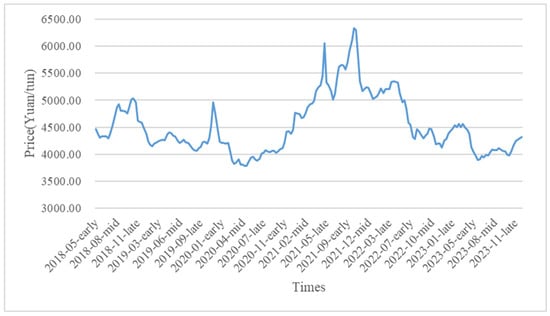
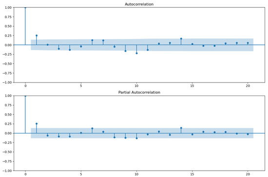
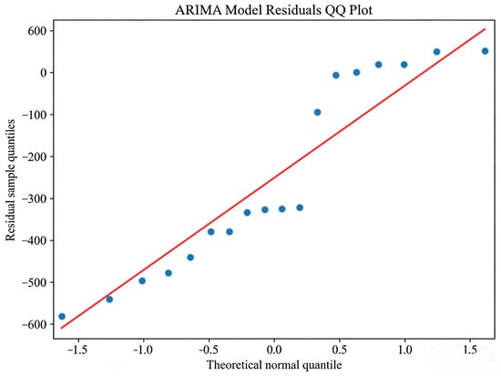
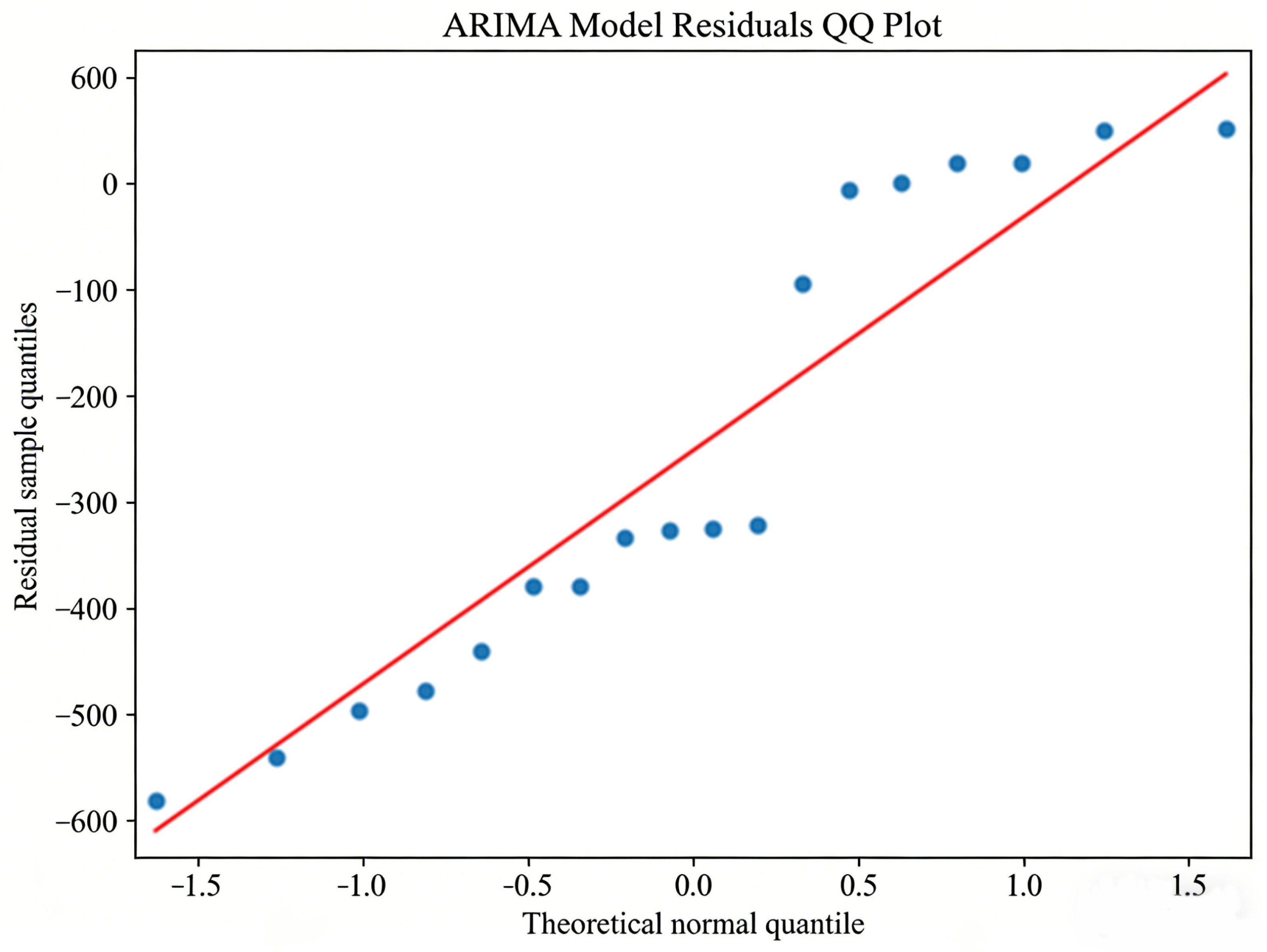
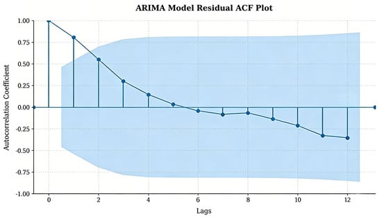
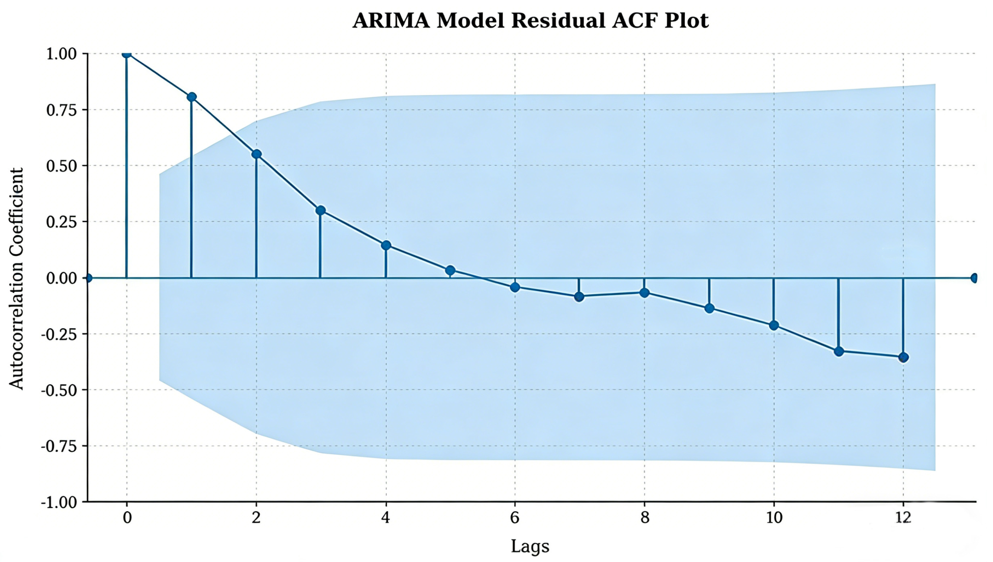
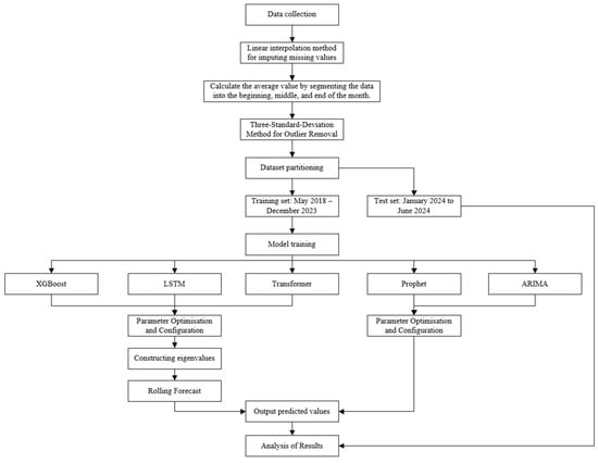
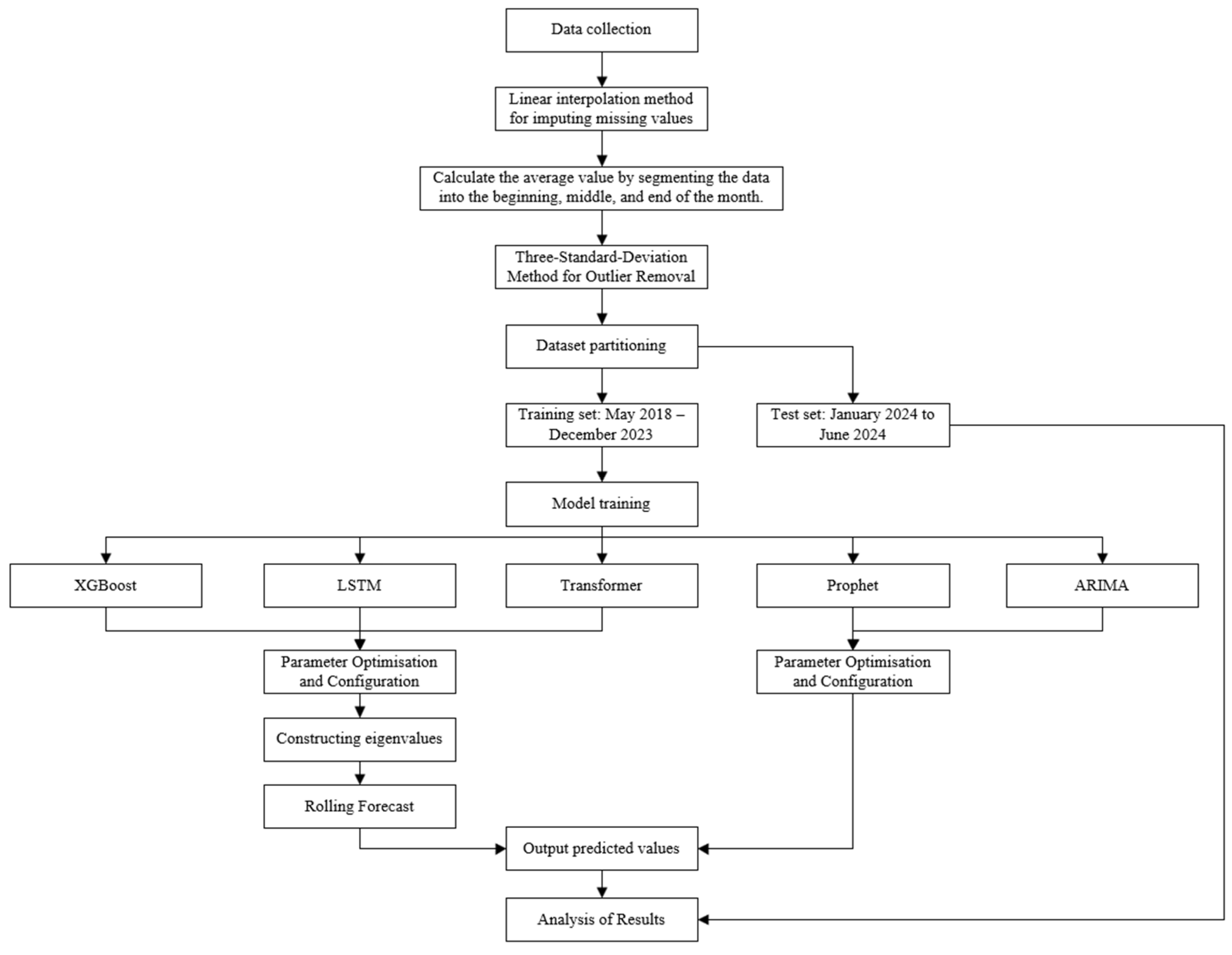
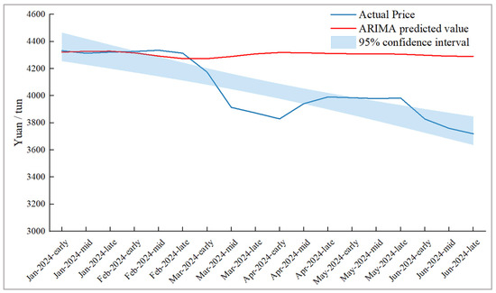
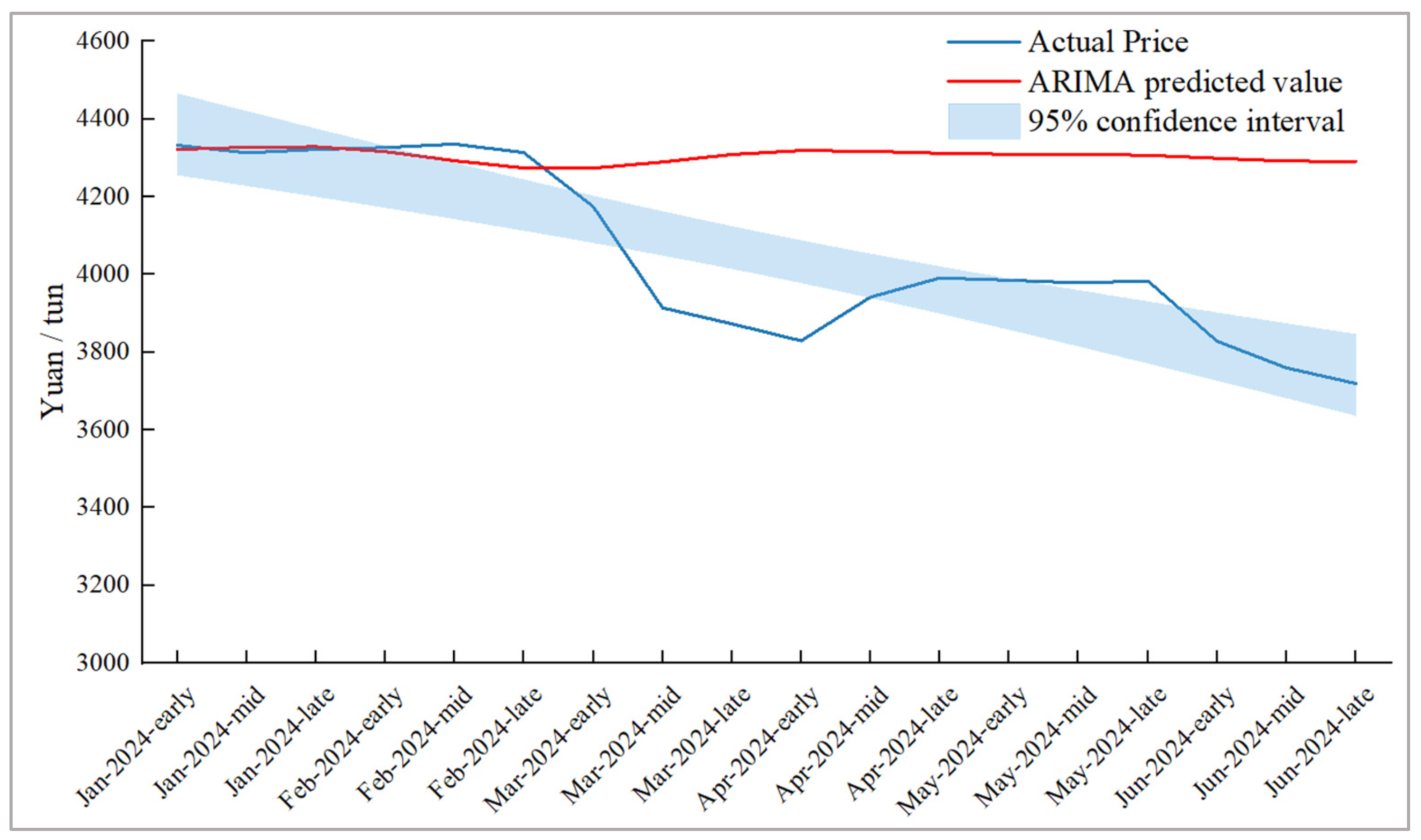
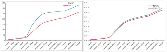
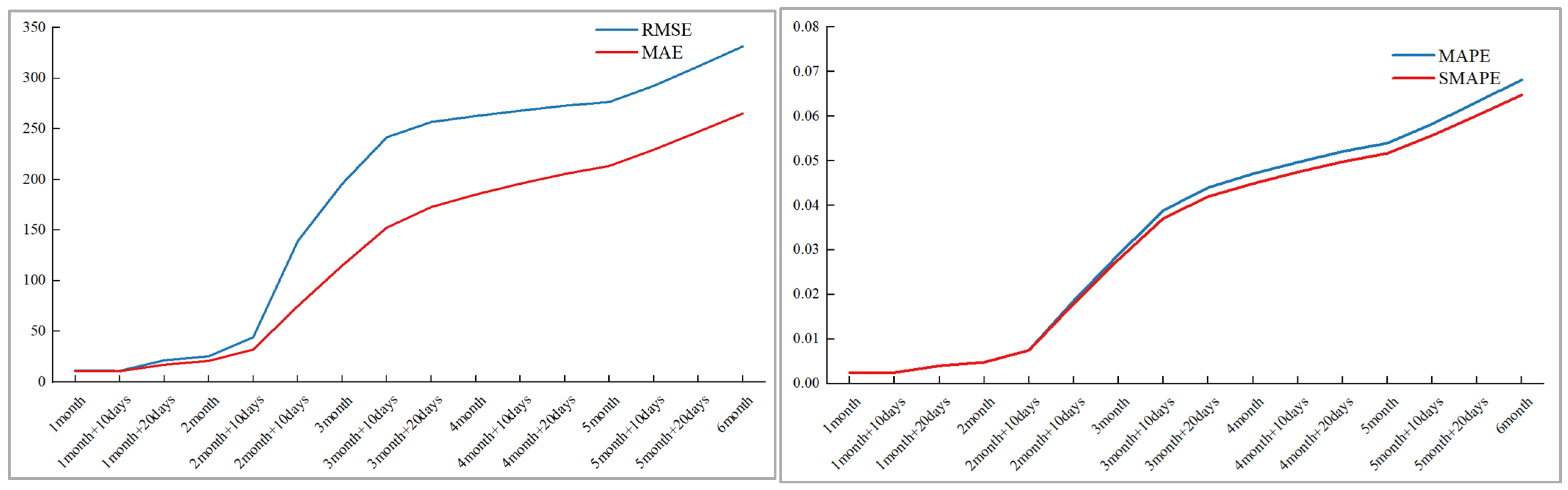
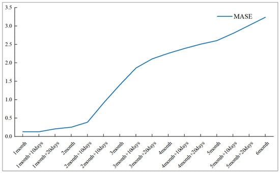
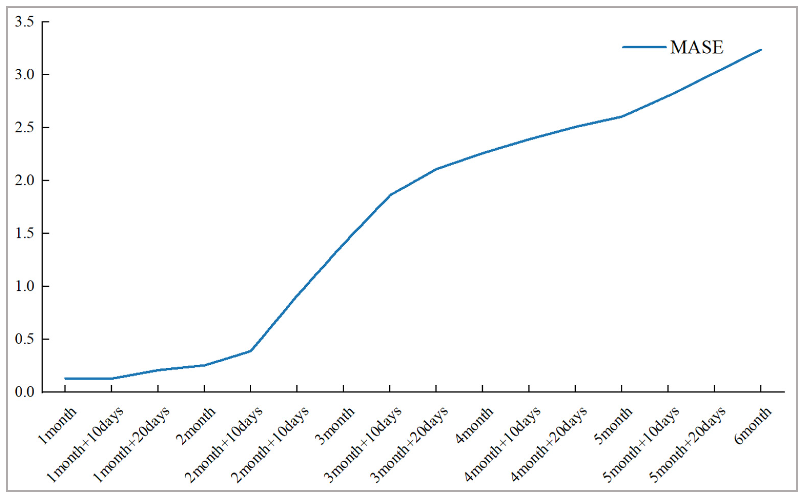
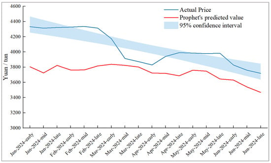
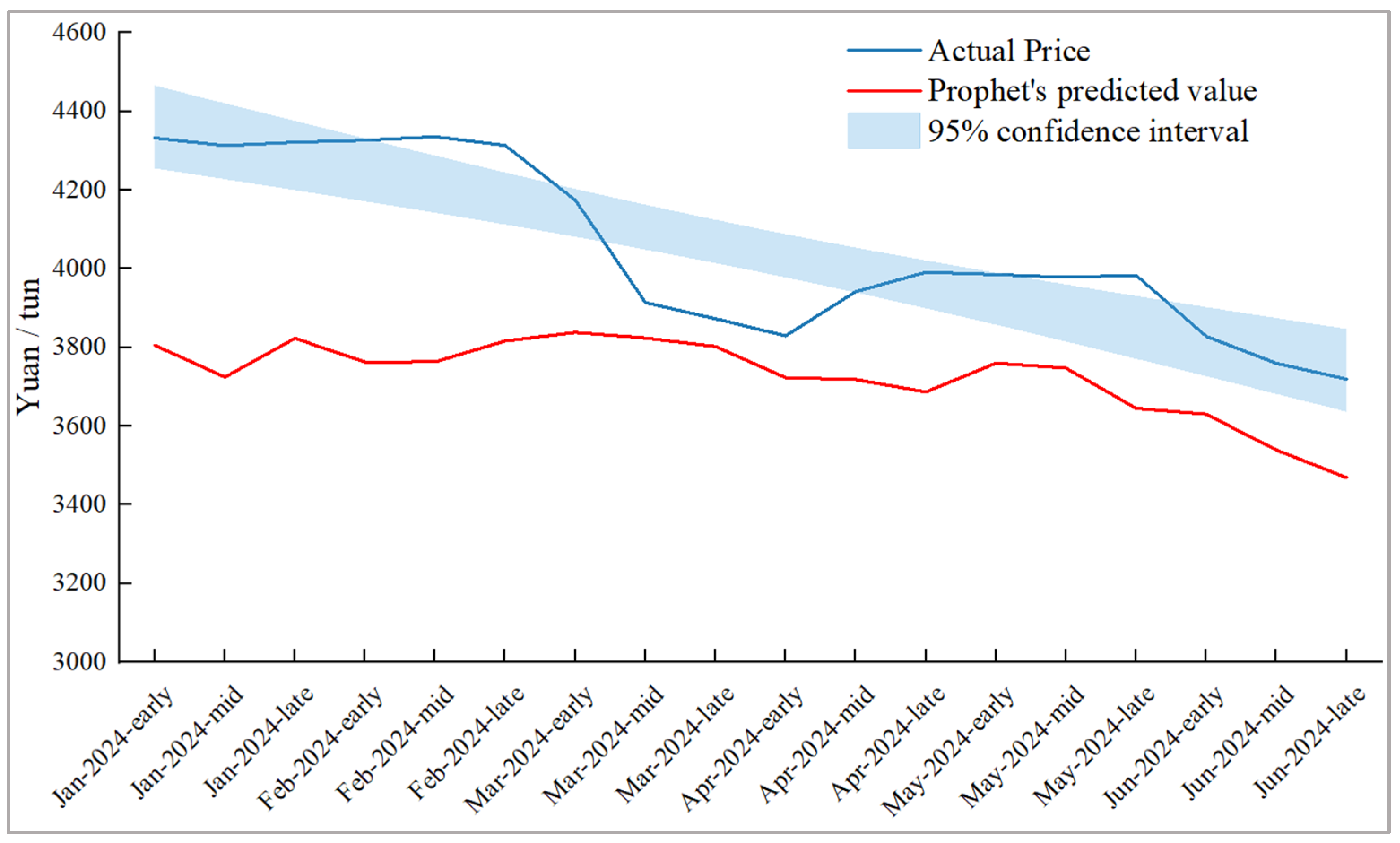
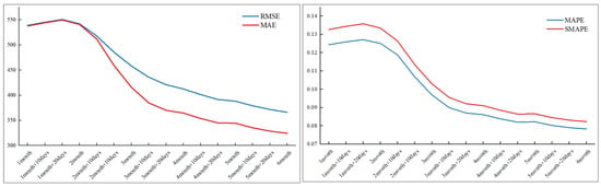
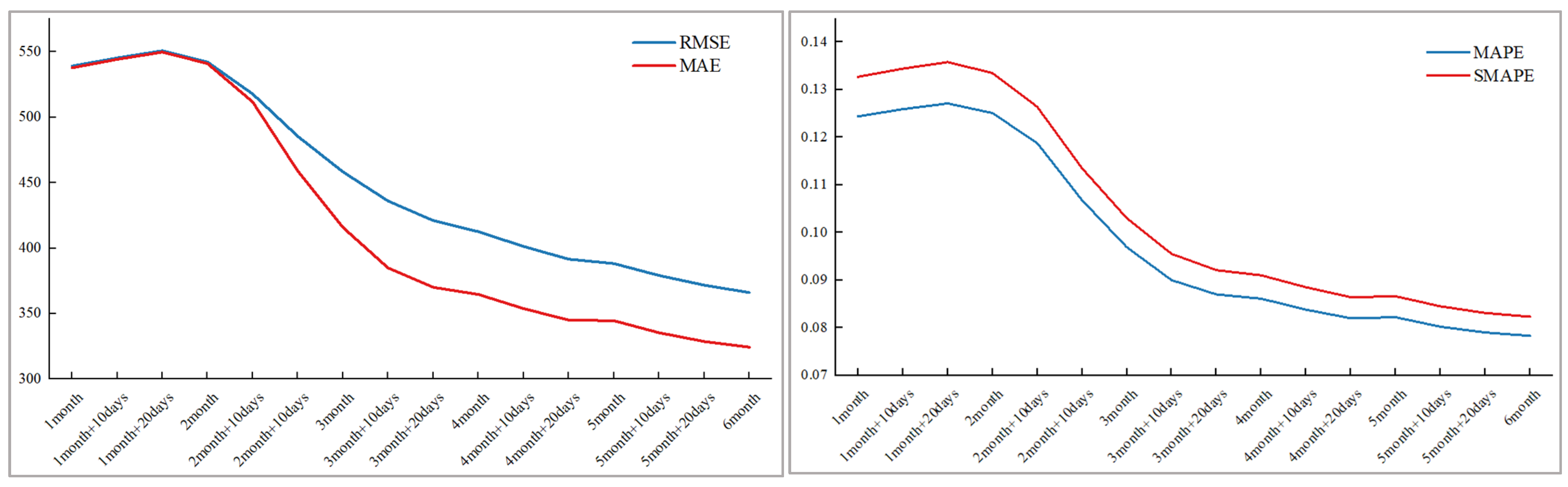
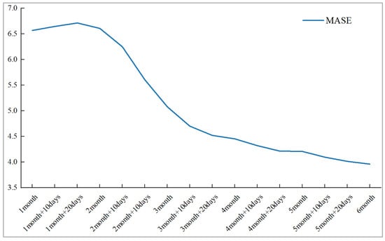
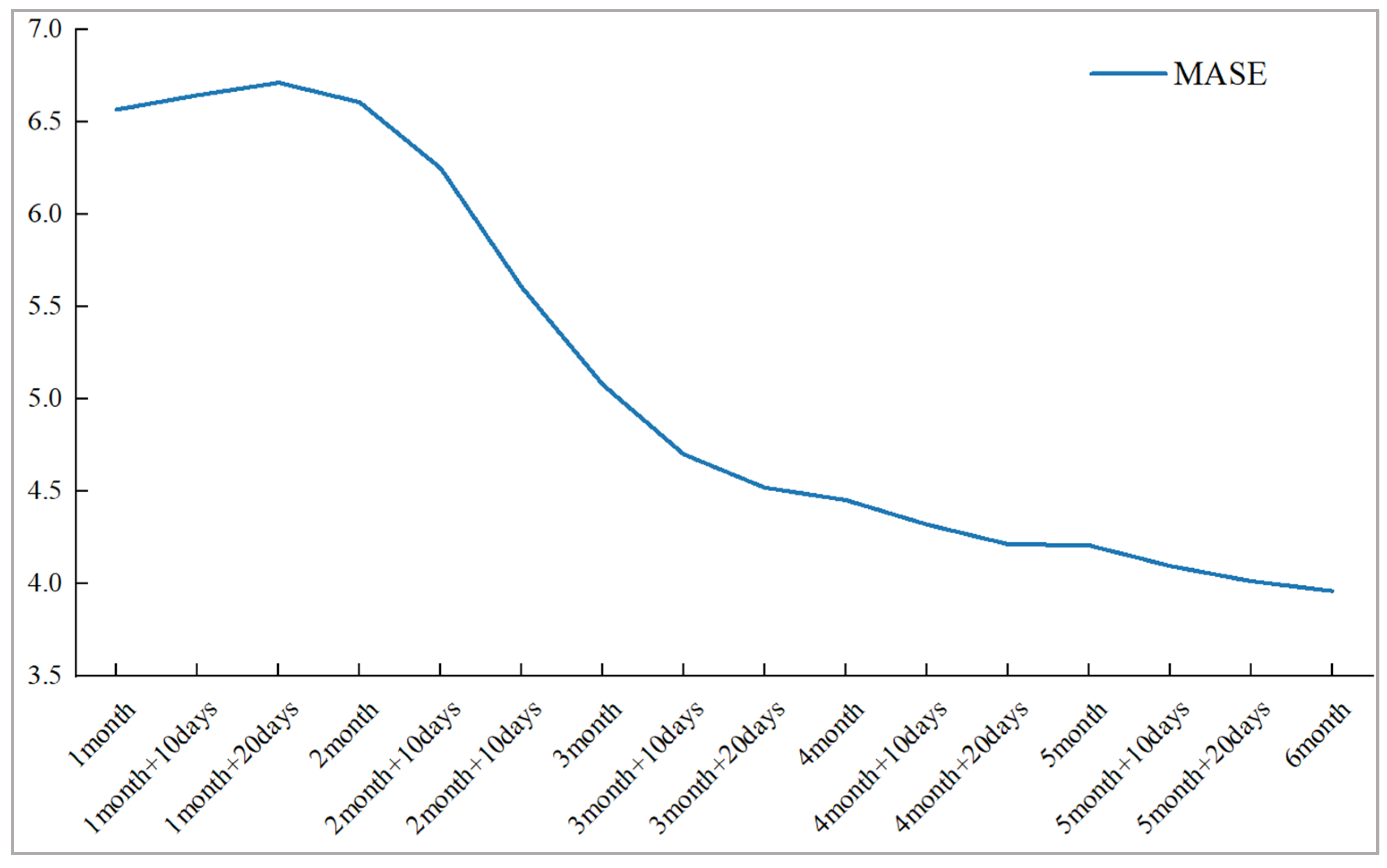
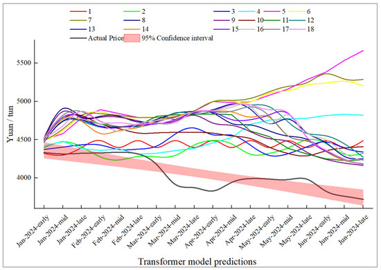
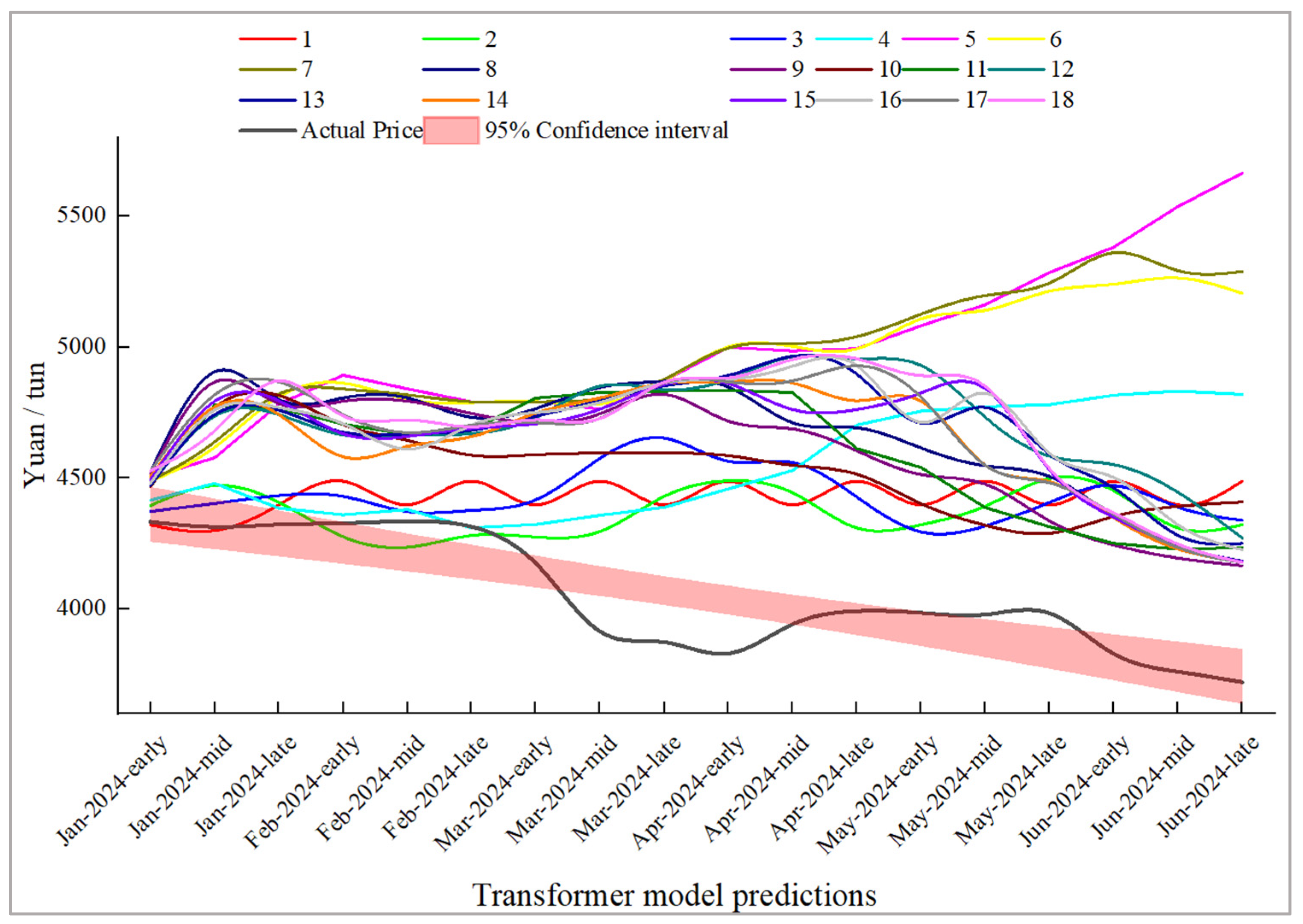
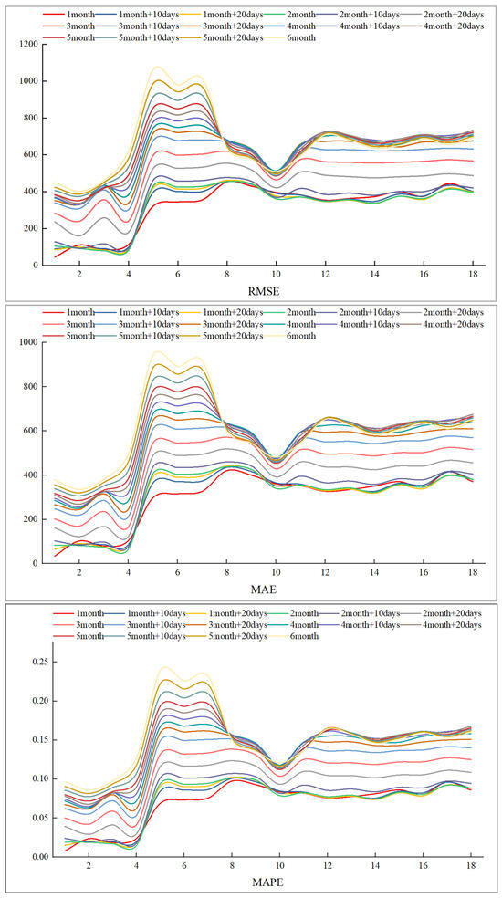
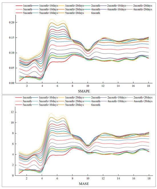
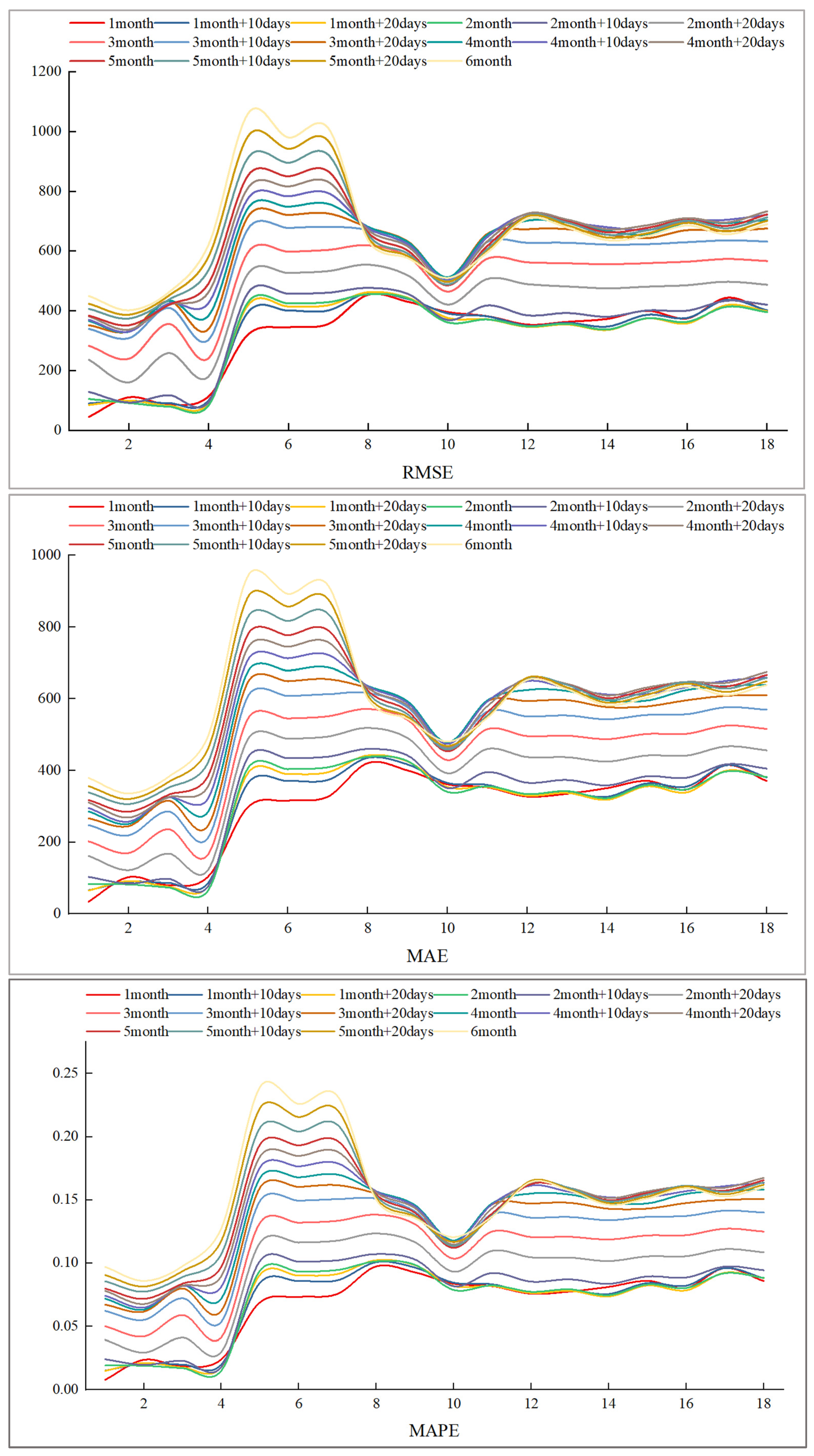
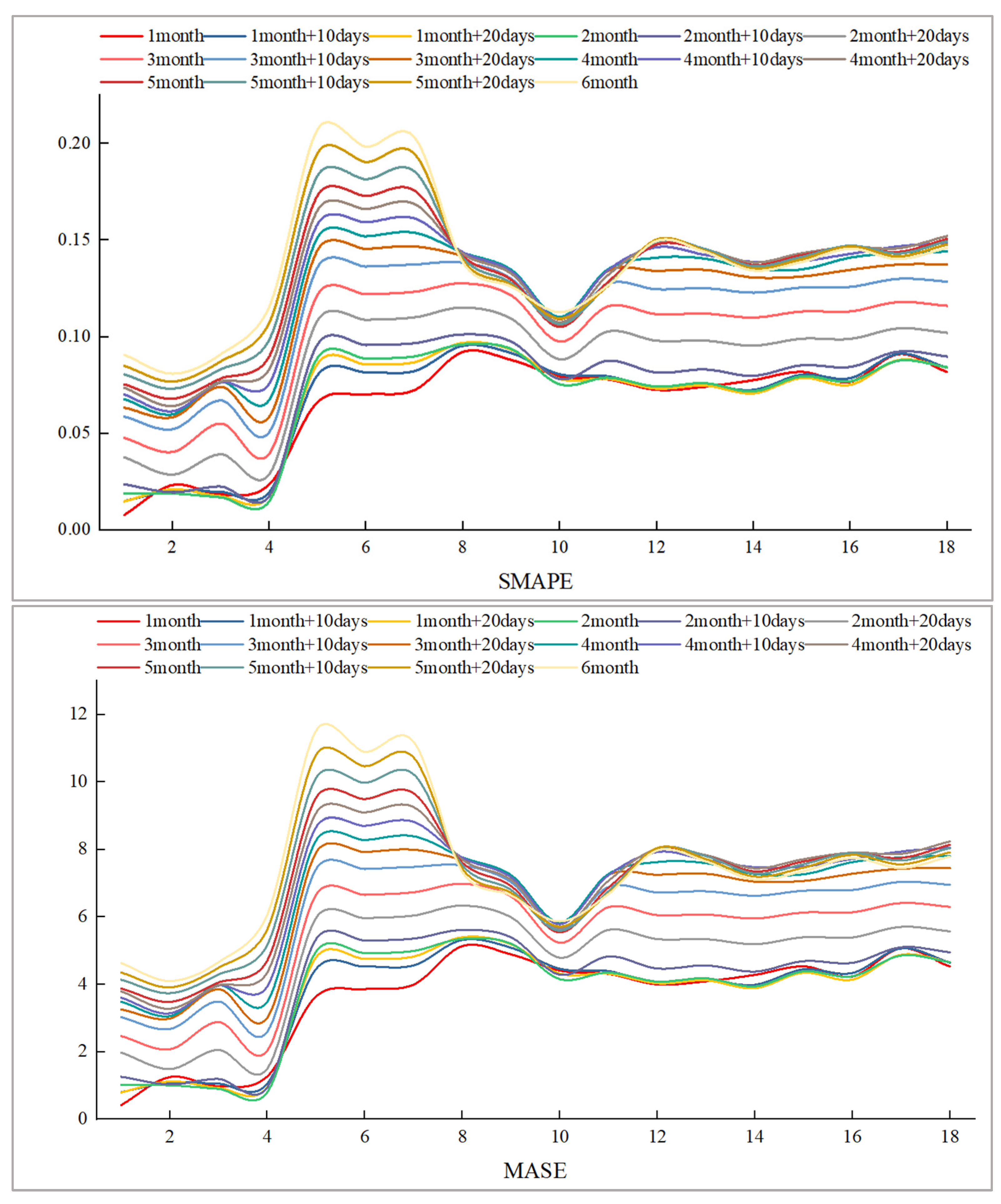
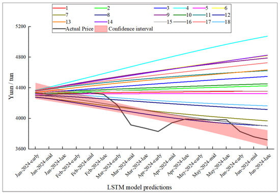
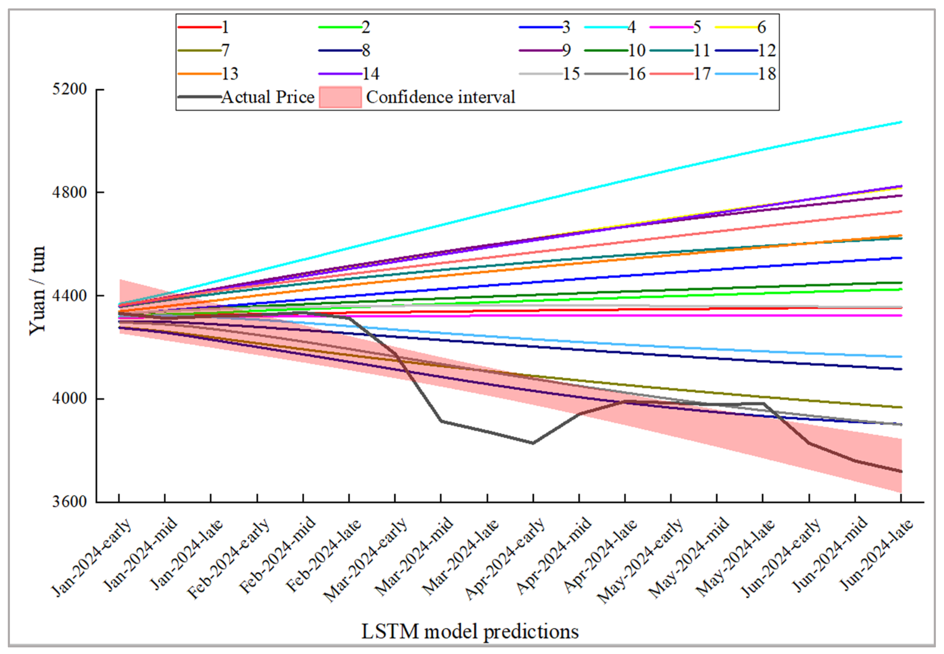
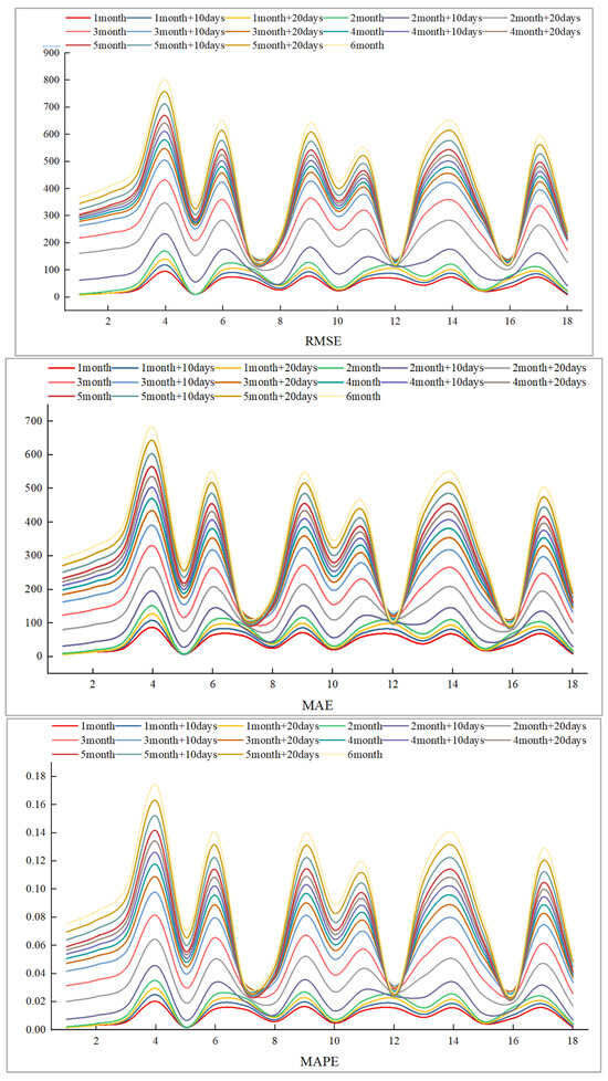
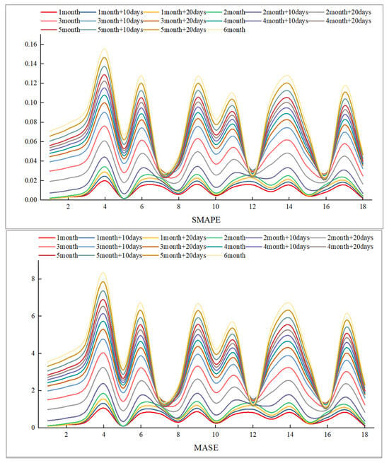
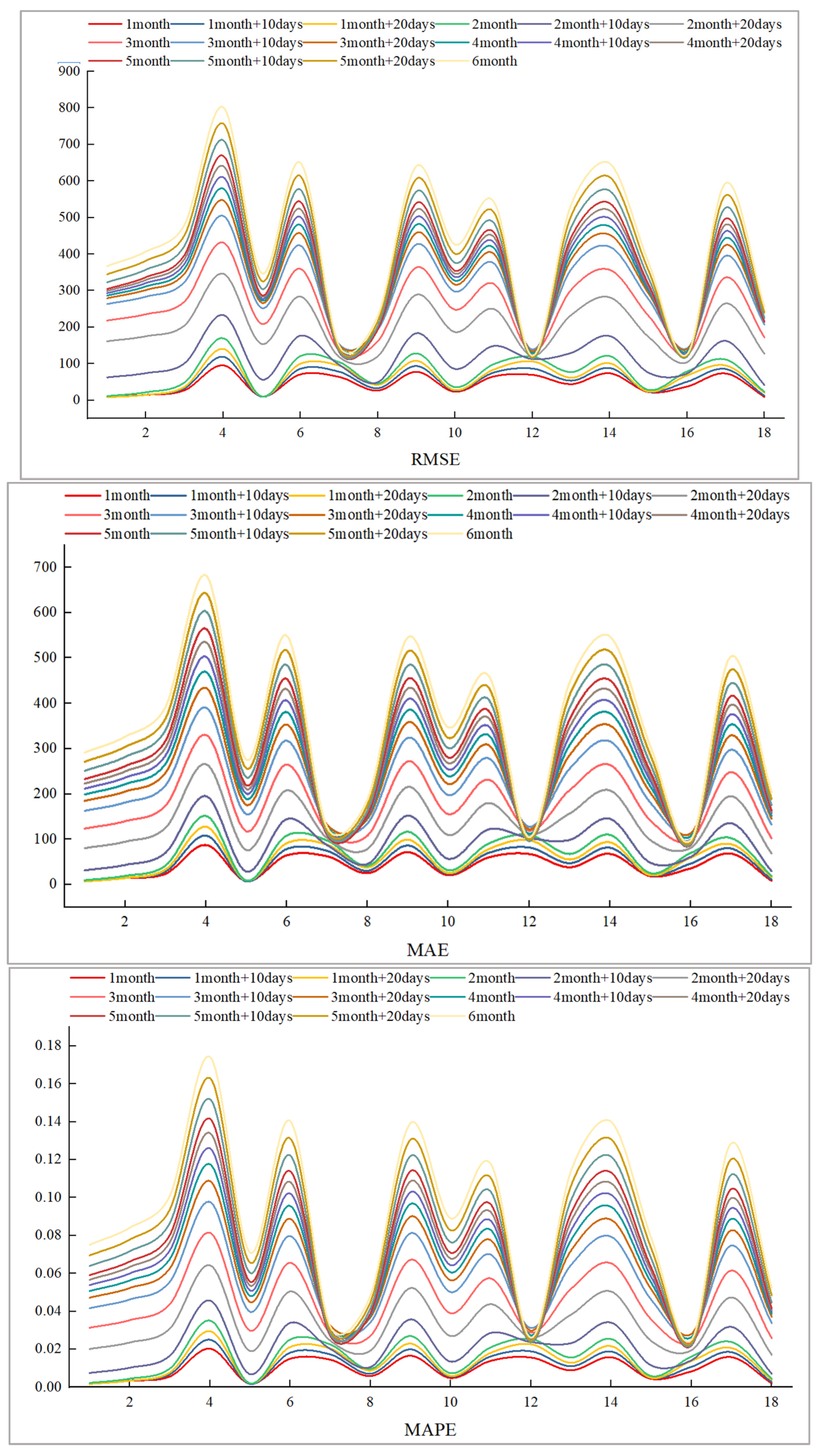
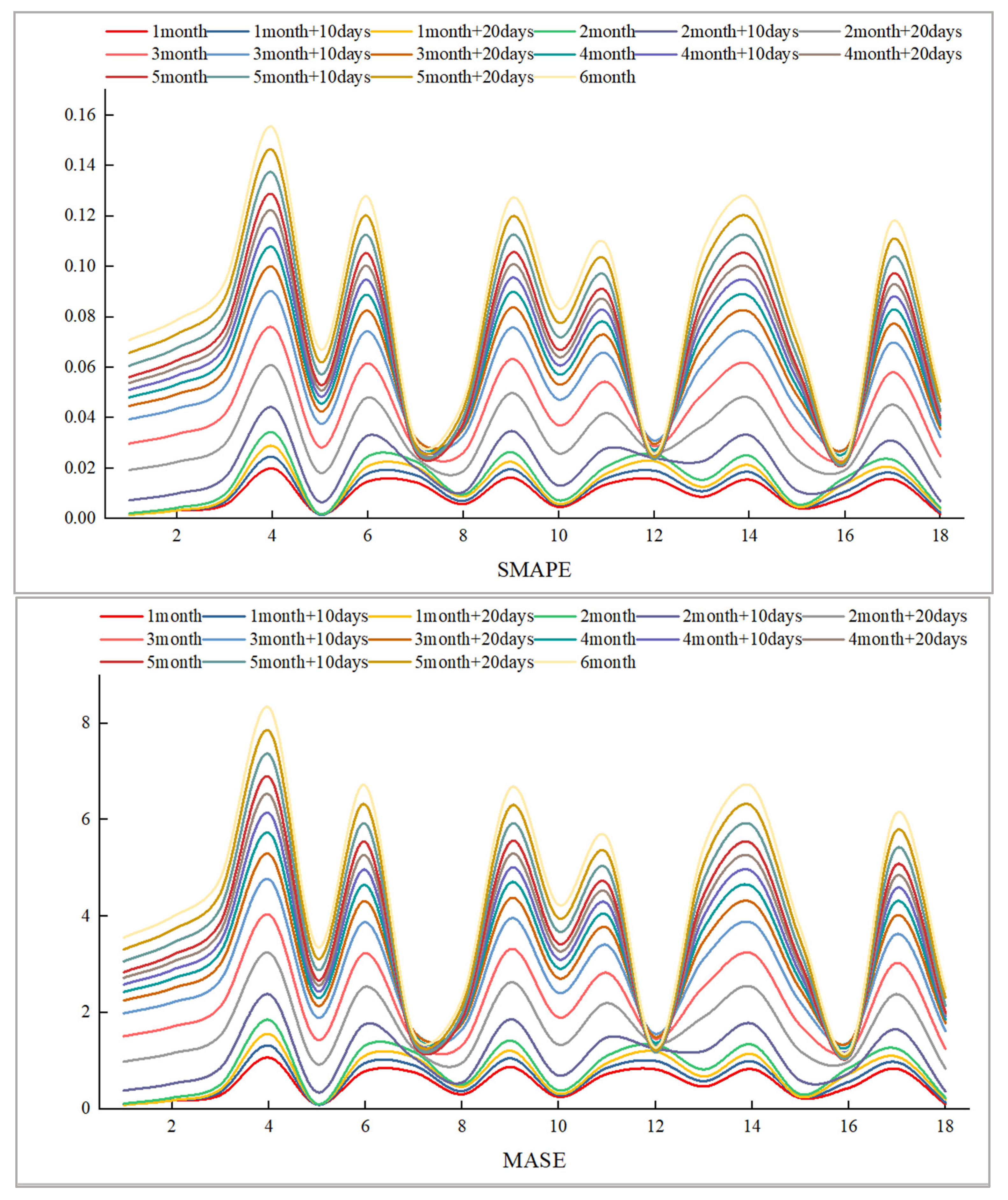
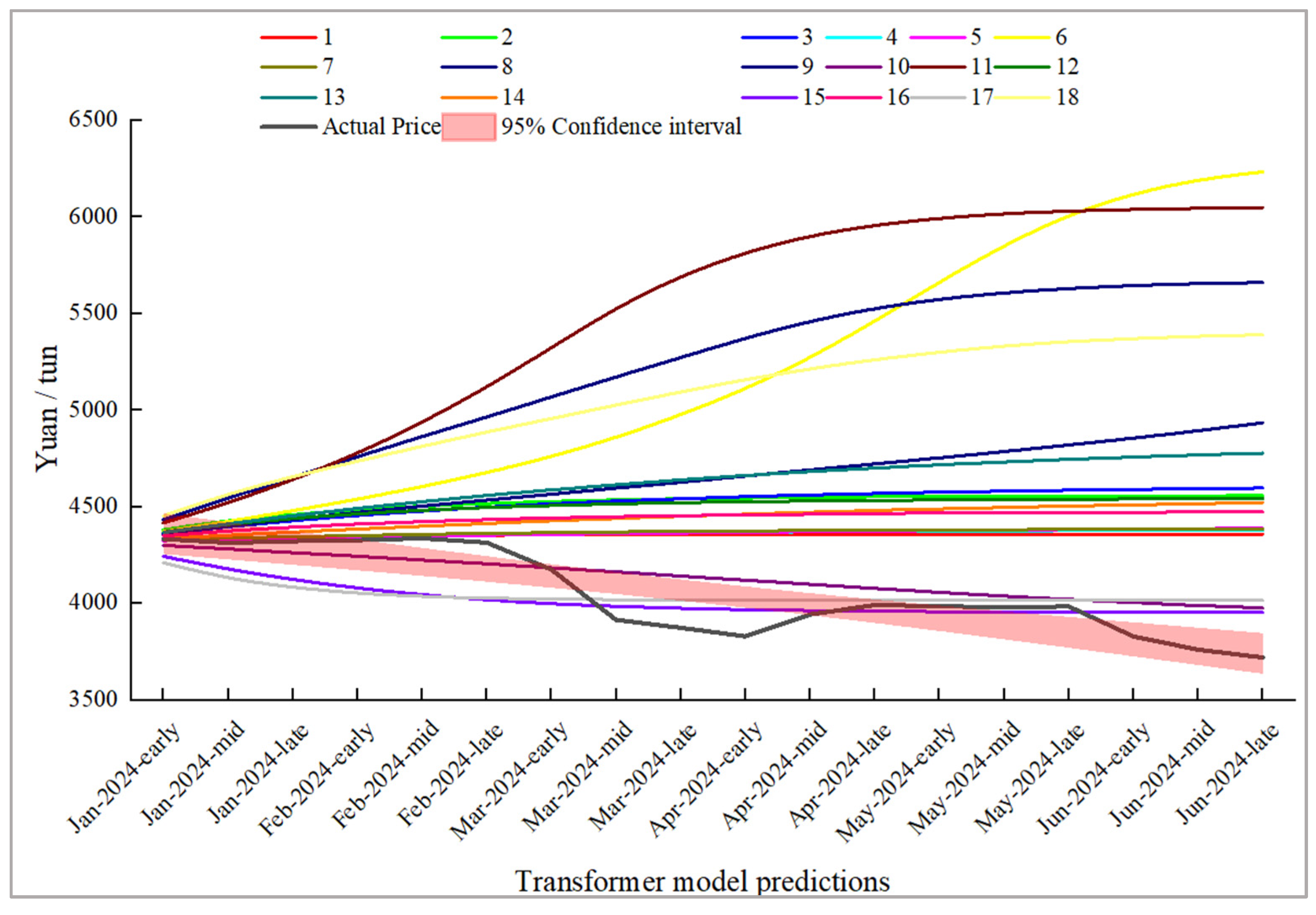
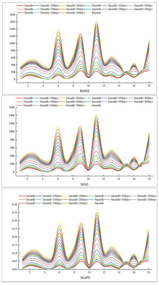
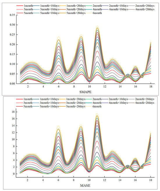
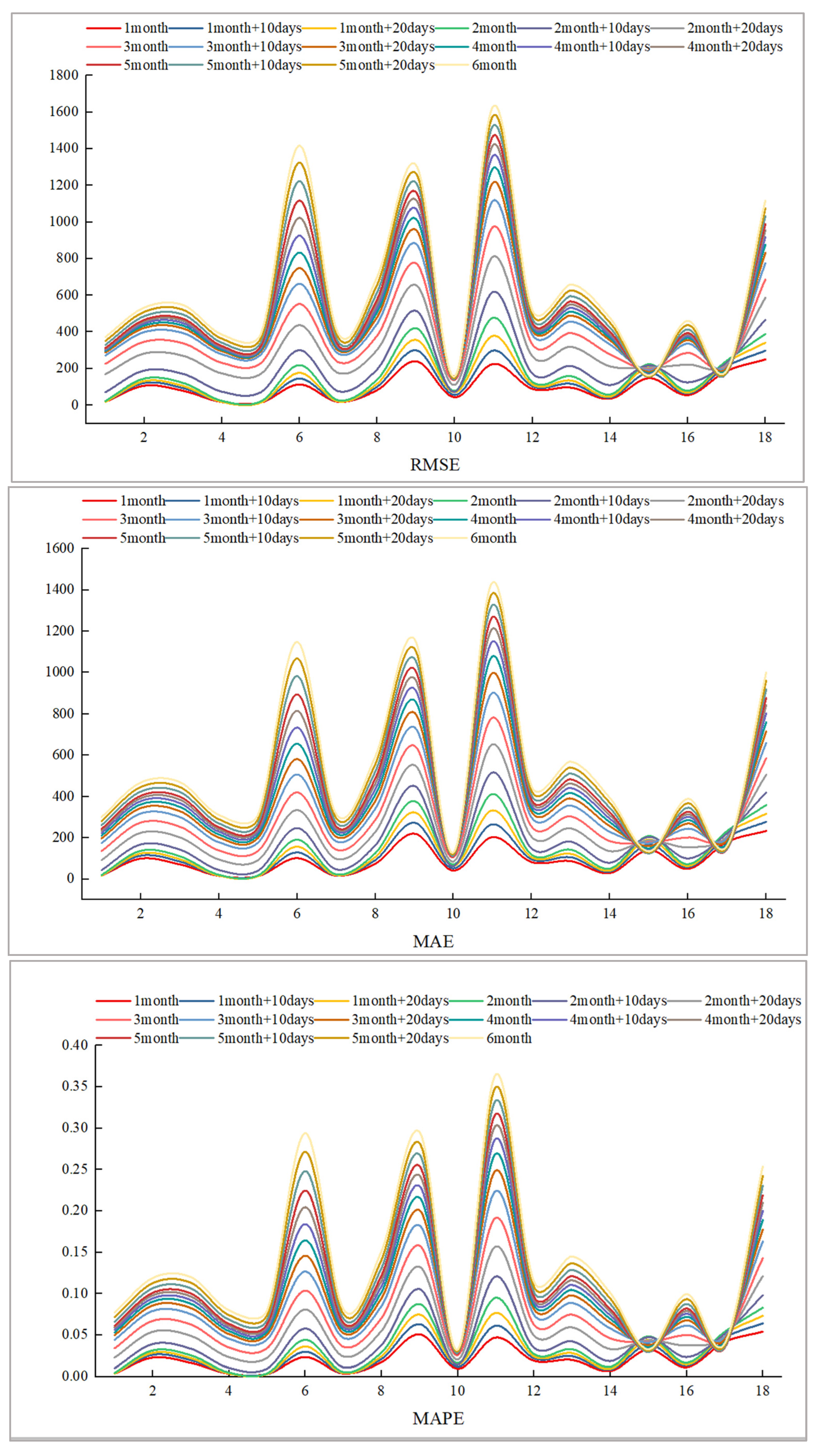
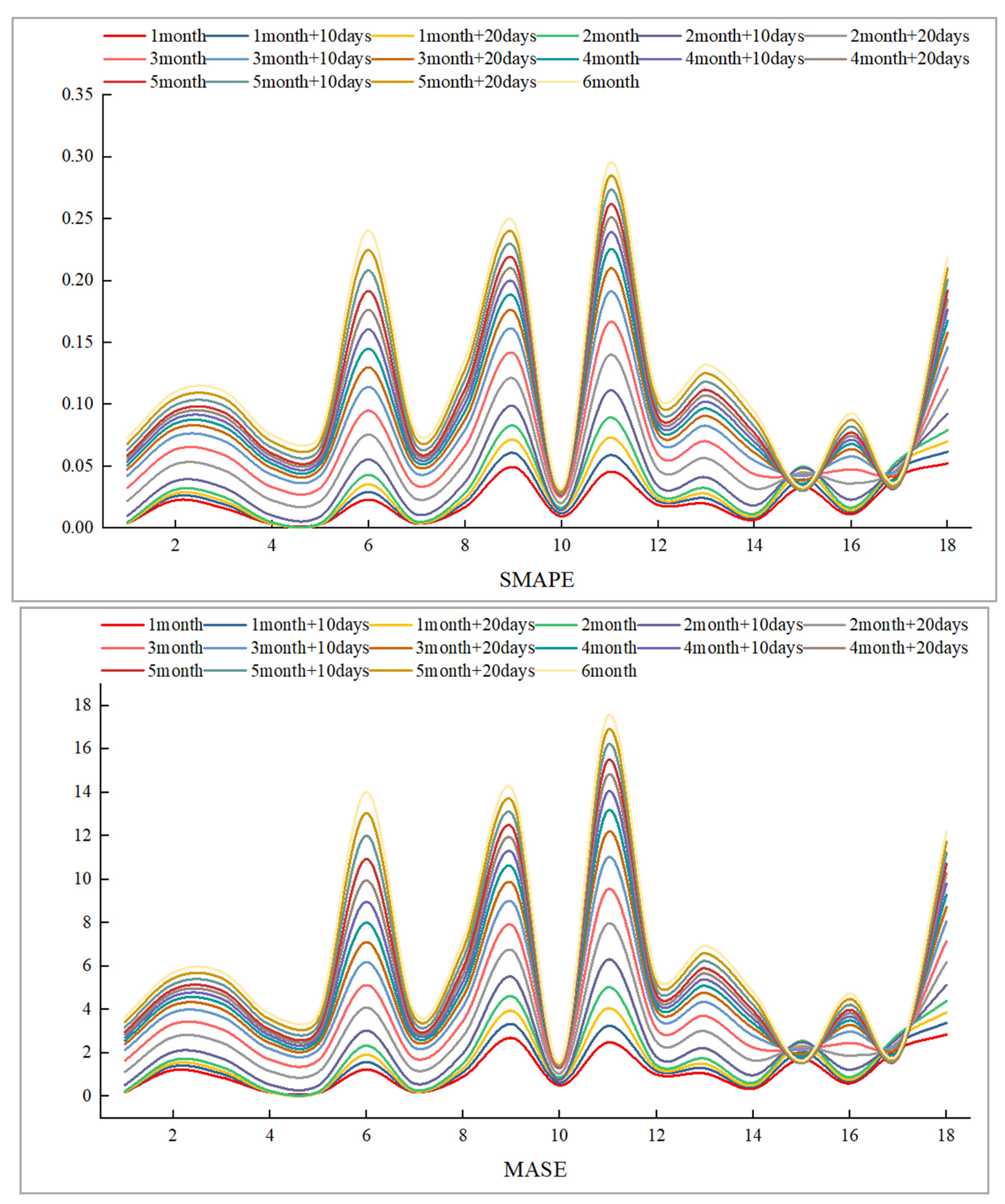
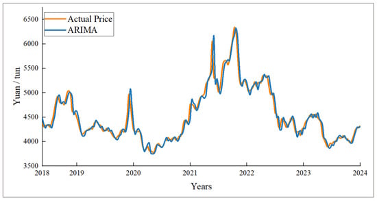
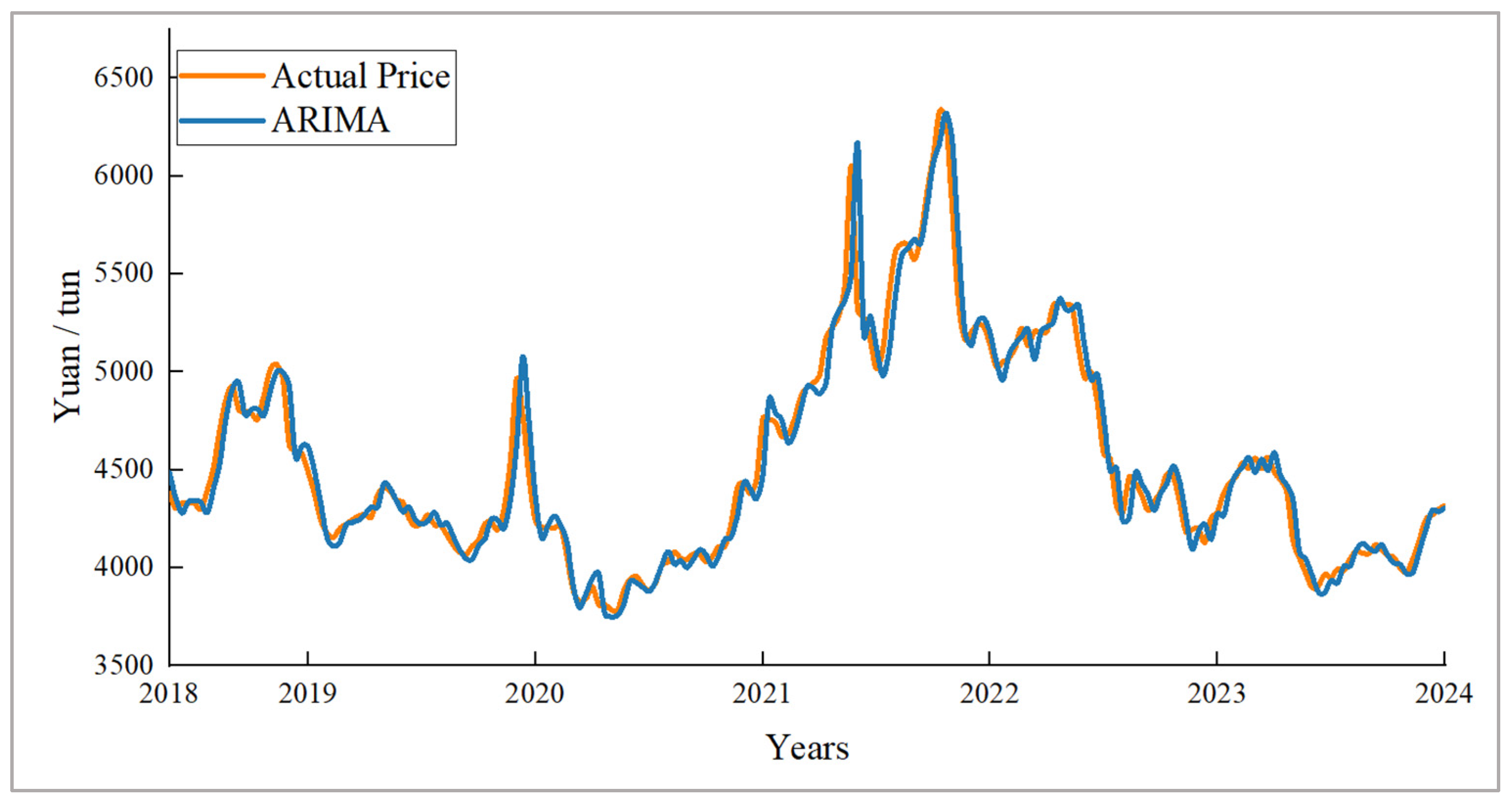
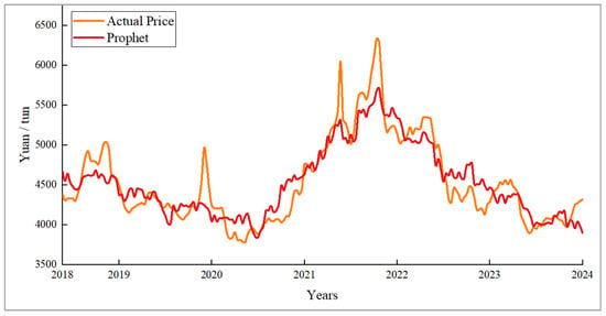
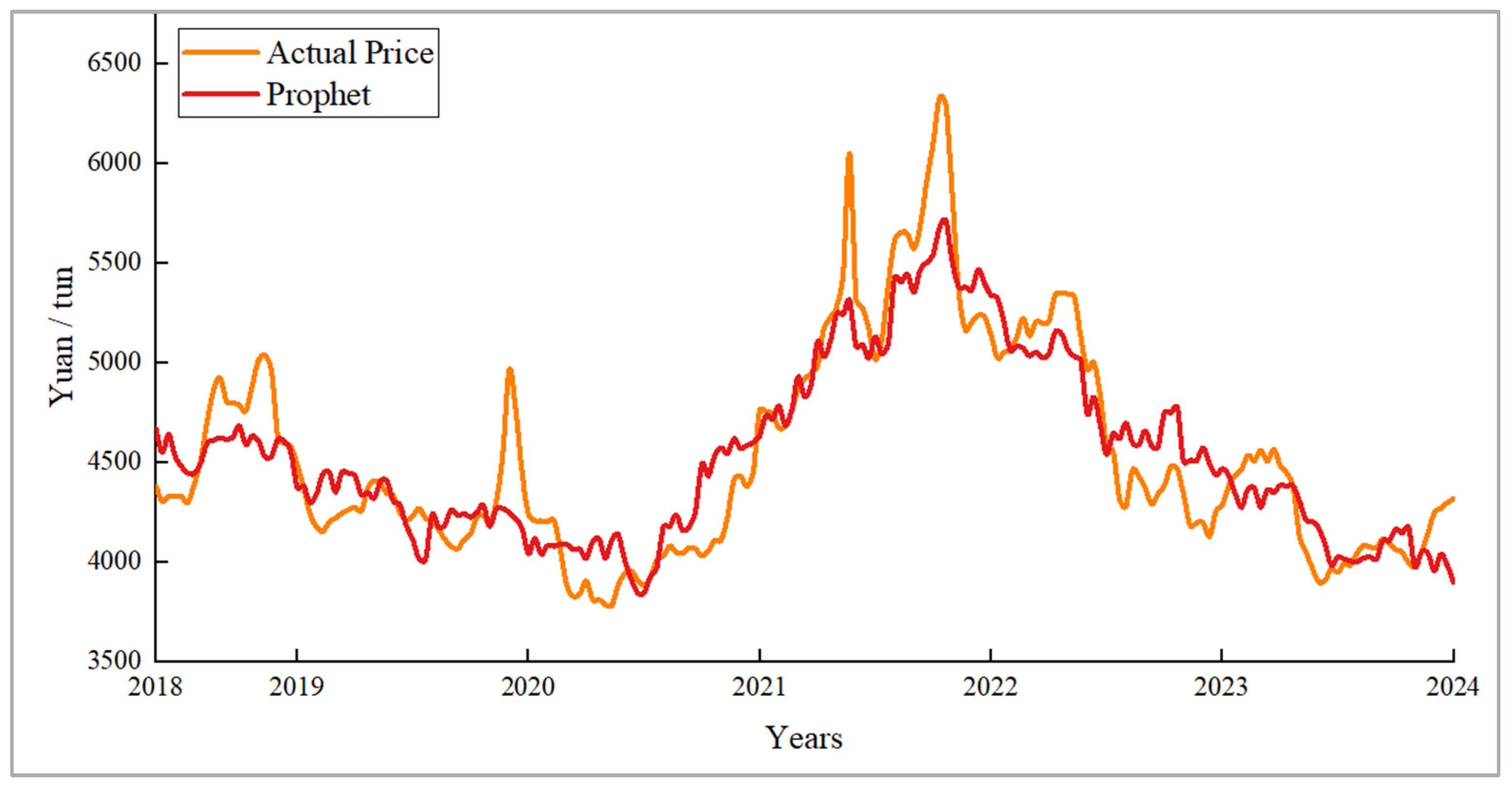
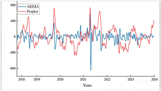
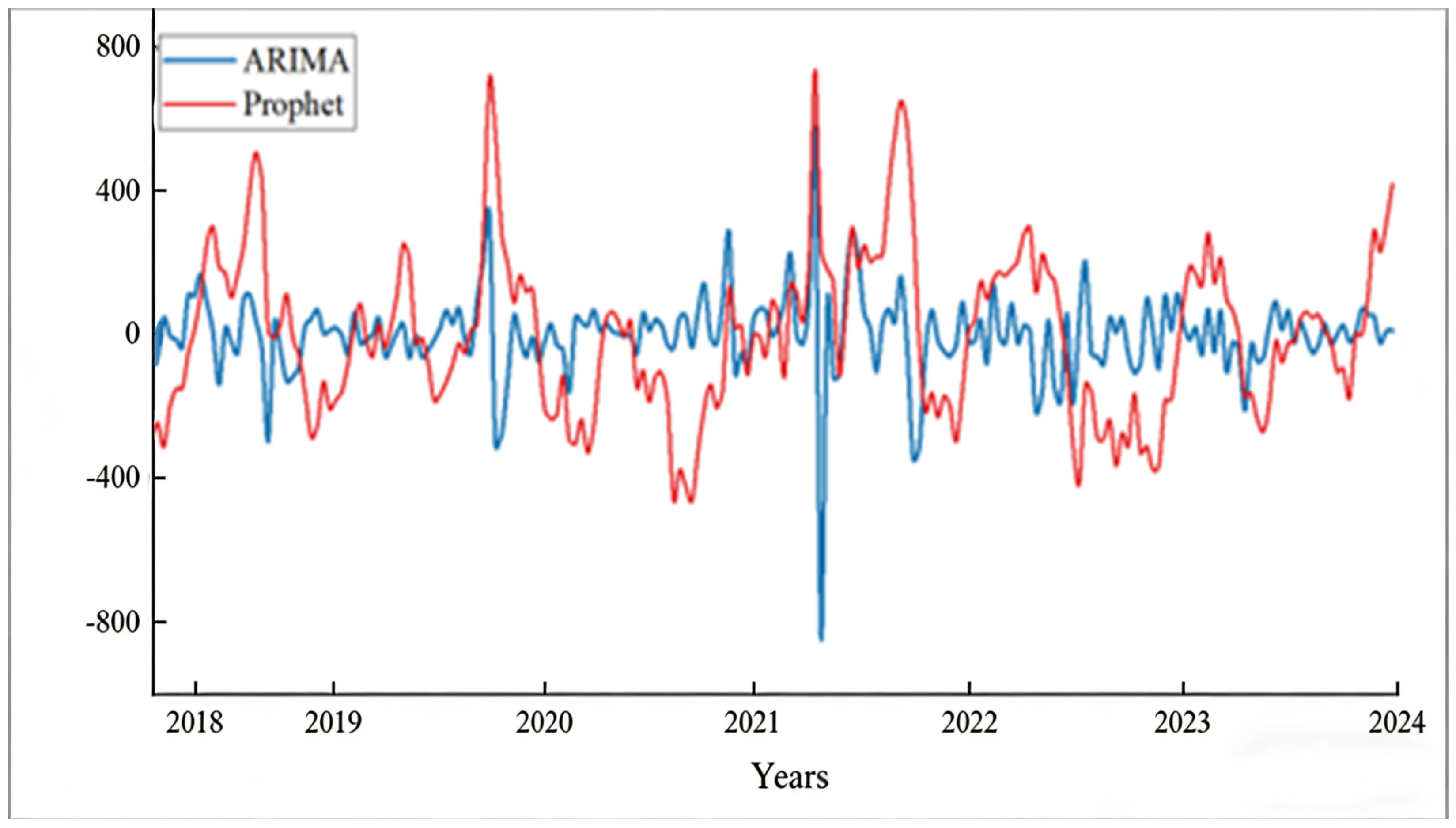
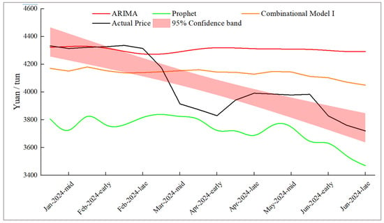
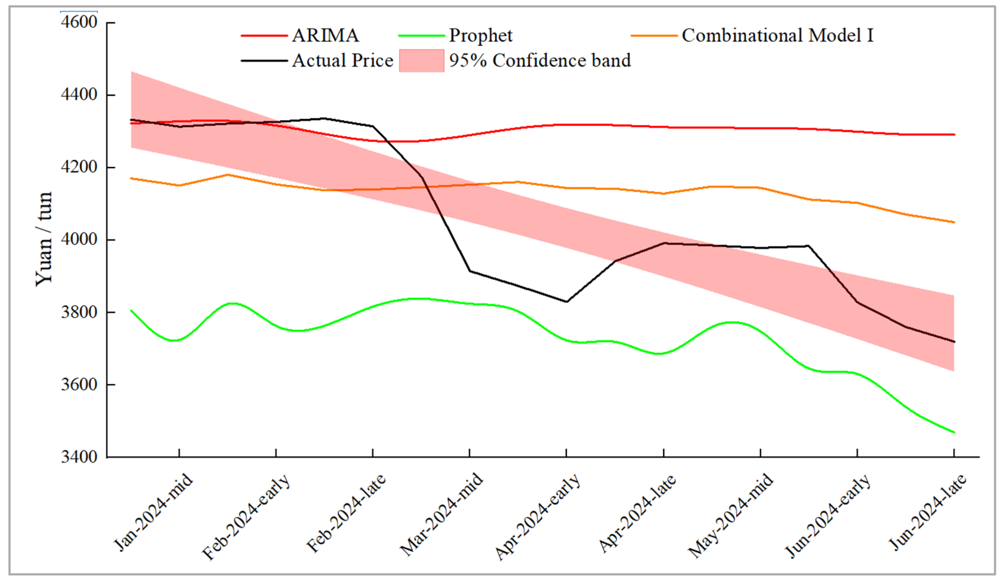
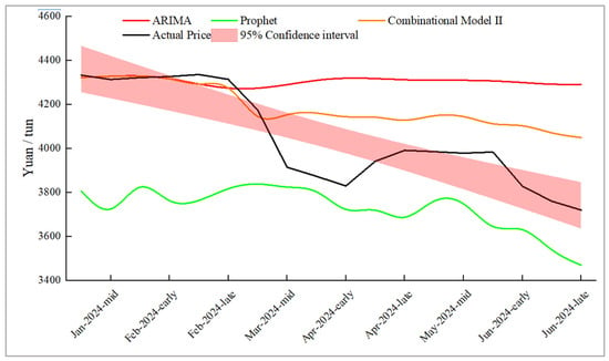
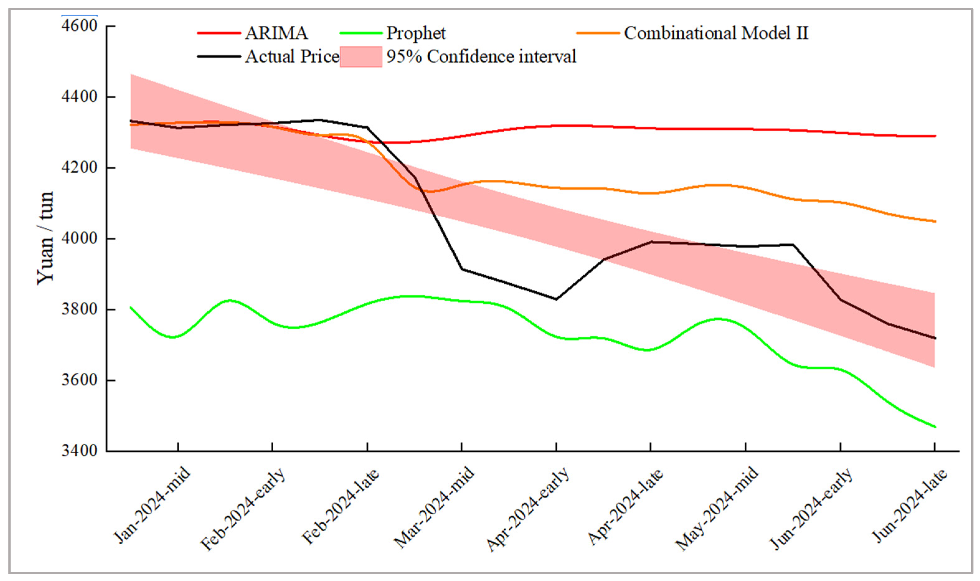

Disclaimer/Publisher’s Note: The statements, opinions and data contained in all publications are solely those of the individual author(s) and contributor(s) and not of MDPI and/or the editor(s). MDPI and/or the editor(s) disclaim responsibility for any injury to people or property resulting from any ideas, methods, instructions or products referred to in the content. |
© 2026 by the authors. Licensee MDPI, Basel, Switzerland. This article is an open access article distributed under the terms and conditions of the Creative Commons Attribution (CC BY) license.