


Abstract
The development of high-efficiency energy dissipation devices is crucial for mitigating the significant threat posed by seismic loads to modern buildings. Therefore, the purpose of this work is to design a novel fluid viscous inerter damper (FVID) and systematically investigate its mechanical performance through theoretical derivations, experiments, and finite element simulations. Furthermore, the impact of FVIDs on the seismic performance of structures is comprehensively evaluated. The advantage of FVID is that under external excitation, the fluid can flow through multiple channels, thereby generating inertial and damping forces to dissipate energy. The theoretical model of FVID’s output force is determined based on FVID’s construction and fluid flow characteristics. The hysteresis performance of the FVID is evaluated through cyclic loading tests, and the influence of the cross-sectional radius and number of turns of the helical tube on its output force is analyzed. By performing finite element simulations of the internal flow field of FVID, the distributions of fluid pressure and velocity at different positions within FVID are analyzed. Based on Simulink, the focus is on investigating the control effect of FVID on structural responses under non-pulse near-field ground motions, pulse-type near-field ground motions, and far-field ground motions. The results indicate that the FVID has a strong energy-dissipation capacity and can effectively reduce structural responses under different types of earthquakes. The cross-sectional radius of the helical tube is a key design parameter that determines the damper’s output force. For highly destructive pulse-type near-field ground motions, FVIDs still exhibit excellent comprehensive performance in the structure.
1. Introduction
In the field of modern engineering, the safety of buildings is still seriously threatened by dynamic loads such as earthquakes. The impact on high-rise buildings, long-span bridges, and large-span spatial structures is particularly prominent. The structural vibration caused by earthquakes may lead to structural damage or even functional failure. For example, the 1985 Mexican earthquake event [1,2], the 1995 Kobe earthquake in Japan [3], and the 1971 San Fernando earthquake event [4] all caused serious damage to local buildings. Therefore, the development of efficient and reliable structural vibration control technology remains a hot research topic in the field of structural seismic resistance [5,6,7,8,9].
Depending on whether the control system requires external energy input, structural vibration control can be divided into passive control [10,11,12], active control [13,14,15], and semi-active control [16,17,18]. Among numerous vibration control strategies, passive control devices, which do not rely on external energy and are easy to maintain, are widely used. In recent years, the use of inerters as passive control components for structural seismic resistance has attracted significant attention from many scholars [19,20,21]. The inerter is an engineering device that controls vibration energy through its inertial element. Its core principle is to use the mass amplification effect to generate an apparent mass thousands of times greater than its physical mass and the negative stiffness effect to optimize system dynamic behavior [22,23,24]. The design concept of inerter was first proposed by Professor Smith in 2002 and subsequently applied to the shock-absorption system of automobiles [25,26]. Due to inerters’ excellent shock-absorbing properties, there has been increasing research on their impact on the seismic performance of structures [27,28,29,30]. For example, Brzeski et al. [31] designed a new type of tuned mass damper that integrates inerters and found that it can significantly suppress the vibration of the main structure over a wide range of excitation frequencies. Gao et al. [32] proposed a negative stiffness inertial damper for multimodal vibration control of cable-stayed bridges. Based on numerical simulations and performance comparisons, it was found that the damper, which can simultaneously utilize the synergistic effects of the negative stiffness device and the inerter, significantly improves the modal damping ratio of structures. De Domenico et al. [33] studied the application of a tuned mass damper inerter with parasitic damping and a fluid inerter-based tuned mass damper for the control of base-isolated building structures. The results of the nonlinear time-history analysis indicate that both systems can significantly reduce the structure’s seismic response. Wang et al. [34] proposed a novel tuned liquid column damper-inerter system for seismic vibration control of single-degree-of-freedom structures. The key conclusion indicates that the damper can reduce structural displacement and acceleration under various actual earthquake records, and significantly improve the performance and stability of vibration control systems. Wang et al. [35] studied the effect of a novel tuned inerter-negative-stiffness damper on structural control performance. The analysis results show that the damper can significantly improve the energy dissipation capacity.
At present, some research has been conducted on inerters for structural vibration control, but further exploration is still needed into their construction and mechanical properties. Especially, there is still a lack of comprehensive research on the mechanical behavior and key design parameters of the viscous inerter damper, which integrates fluid viscous damping characteristics and inertial systems. Therefore, this study aims to design and investigate a new type of fluid viscous inerter damper (FVID), and to study its comprehensive mechanical performance through theoretical derivation, experimental testing, and finite element simulation. In addition, numerical simulations are used to evaluate the impact of FVID on improving the seismic performance of structures. The characteristic of FVID is that under external excitation, the fluid can flow through multiple channels, including damping orifices on the piston and the helical channel of the helical tube. This process generates inertial and damping forces to achieve effective energy dissipation. The theoretical mechanical model of FVID is proposed based on the structural details and internal fluid flow characteristics of the designed damper. The hysteresis performance of FVID is comprehensively investigated through cyclic loading tests, and the influence of the cross-sectional radius and number of turns of the helical tube in FVID on the output force is evaluated by analyzing the hysteresis curve of the damper. Furthermore, theoretical results are compared with experimental results to validate the accuracy of the theoretical mechanical model of FVID. The finite element model of the internal flow field of FVID is established by Fluent software, with a focus on analyzing the distributions of fluid pressure and flow velocity. The variation trends of velocity and pressure along the fluid flow direction in the internal cross-sections of spiral and damping orifices are discussed in detail. The rationality and feasibility of the designed damper are verified by comparing the finite element results, experimental results, and theoretical calculation results. The dynamic simulation of the three-story benchmark building equipped with FVIDs is carried out by Simulink. In addition, the seismic reduction effect of FVIDs on the structure under non-pulse near-field ground motions, pulse-type near-field ground motions, and far-field ground motions is investigated. Six performance indicators are considered to further quantitatively evaluate the impact of FVID on the seismic performance of structures under different types of earthquakes. The main innovations of this study are as follows: (1) a new multi-channel FVID is proposed, which achieves the parallel integration of the helical tube and damping orifices within the device. Based on this new parallel flow channel design, the inertial force generated by the helical tube and the viscous damping force generated by the damping orifices can be simultaneously produced in each working cycle. This design can significantly improve the energy dissipation efficiency of the damper. (2) Through theoretical derivation, experimental testing, and CFD simulation, the mechanical characteristics and internal flow field mechanism of the FVID are comprehensively revealed, and the analysis results confirm its excellent energy dissipation ability. (3) Based on the Simulink platform, the control effect of the FVID on building structures under different types of seismic waves is systematically evaluated, and the results show that the FVID can effectively improve the seismic performance of the structure. Unlike fluid inerters that can only generate inertial force or viscous dampers that can only generate damping force, the FVID has a unique working mechanism of parallel coordination between inertial and damping forces. This mechanism ensures that fluid flows simultaneously through the helical tube and damping orifices in each working cycle, allowing the FVID to simultaneously generate inertial force and viscous damping force for energy dissipation. The practical benefit of this new working mechanism is that compared with a single energy dissipation mechanism, the FVID can exhibit more stable and efficient energy dissipation characteristics in practical engineering applications. The research results of this paper can provide new feasible solutions for vibration control of building structures.
2. Design Method and Mechanical Theory of FVID
2.1. Design Method of FVID
The inerter is an acceleration-related structural control component. It often needs to be combined with springs and dampers to achieve specific energy dissipation. Therefore, a new type of FVID is proposed in this paper, which combines the advantages of the external helical-tube hydraulic inerter and the orifice-type viscous damper. The FVID possesses both mass amplification effects and viscous damping characteristics. It consists of a main cylinder, an auxiliary cylinder, a cylinder head, a piston, four hollow screws, and a helical tube, as shown in Figure 1.
Figure 1.
The basic construction diagram of FVID.
In Figure 1, the fluid is filled in the helical tube, the damping orifices on the piston, and the internal cavity formed by the connection of the main cylinder and the cylinder cap. When the piston rod is subjected to an external force, the fluid in the internal cavity formed by the connection of the main cylinder and the cylinder cap flows through the damping orifices on the piston, and simultaneously flows through the helical tube, thereby generating inertial force and damping force.
In the designed damper, the main cylinder and cylinder head are connected to form an inner cavity. The piston is placed in the inner cavity, and its surface is provided with threaded holes for installing hollow screws. The hollow area of the screw is a damping orifice with a circular cross-section. This channel is used to allow fluid to flow between chambers, thereby generating the damping force. The piston rods are fixed on both sides of the piston. There are threaded holes on the walls of the main cylinder and the cylinder head for connecting the helical tube. The auxiliary cylinder is connected to the main cylinder to accommodate and protect the exposed portion of the piston rod. At the same time, an exhaust hole is set on the outer surface of the auxiliary cylinder to balance the pressure difference between the inside and outside of the cylinder, thereby avoiding the pressure imbalance caused by the vacuum effect. In addition, the fluid is injected into the inner cavity through the oil-injection hole in the cylinder head. Annular grooves are located in the mating surfaces between the main cylinder and the piston rod, and between the cylinder head and the piston rod. These grooves are designed to accommodate the support rings and seal rings. The support ring can reduce the compression gap between the sealing ring and the piston rod, thereby avoiding wear between the piston rod and the cylinder body. In addition, there are annular grooves on the piston’s outer surface for installing guide rings and sealing rings. The sealing ring prevents liquid leakage between the two chambers, thereby avoiding a reduction in chamber pressure. The guide ring guides the piston in a straight line, preventing it from deviating under uneven external forces. In this paper, the function of the helical tube is not to increase stiffness, but to provide damping force and inertial force. When the fluid in the FVID flows through the helical tube, corresponding damping and inertial forces are generated, thereby achieving the function of energy dissipation.
2.2. Mechanics Principle of FVID
The core energy-dissipation principle of the designed damper is the conversion of kinetic energy into thermal energy. Under external loads, the piston rod drives the piston to move relative to the cylinder. Then the viscous medium flows inside the cavity through hollow screws and helical tubes, which can provide the viscous resistance and inertial forces. In addition, the friction force between the piston and the inner wall of the cylinder is generated due to the movement of the piston. To investigate the mechanical model of the designed damper, the force analysis of the FVID is performed. The analysis assumes that the piston rod moves to the left under the external load, and the force analysis of FVID is shown in Figure 2. According to Newton’s second law, the force balance relationship of FVID can be obtained:
where F is the external load acting on the piston; Fch and Fach represent the damping force and inertial force generated by the flow of the fluid medium in a helical tube, respectively; Fd is the damping force generated by the flow of the fluid medium in the hollow screws; f1 is the frictional force between the piston and the inner wall of the cylinder; Fac is the inertial force generated by the flow of the fluid medium in the cylinder cavity; Fam is the inertial force generated by the movement of the piston.
Figure 2.
Mechanical analysis of FVID.
When the fluid medium circulates in the helical tube and hollow screws, the viscous friction between the fluid and the walls of the helical tube and the damping orifices causes pressure loss. The viscous resistance generated during this process can be expressed as:
where p2 is the fluid pressure inside the left chamber of the cylinder, p1 represents the fluid pressure in the right chamber of the cylinder, Ap is the actual working area of the piston, which can be calculated by subtracting the cross-sectional area of the piston rod from the cross-sectional area of the cylinder’s inner cavity.
2.2.1. Analysis of Damping Force
- The damping force Fch generated by the flow of the fluid medium in the helical tube;
Based on reference [36], the pressure loss caused by the flow of the fluid medium in a helical tube can be roughly estimated as follows:
where fF is the Fanning friction coefficient, Re is the Reynolds number, lch is the length of the helical tube after stretching, μ is the dynamic viscosity of the fluid medium, u is the average flow velocity of the fluid medium inside the helical tube. Dh is the hydraulic diameter, which refers to the ratio of four times the flow cross-sectional area to the wetted perimeter.
According to the conservation of the liquid volume, it can be concluded that:
where Qp is the flow rate of the liquid in the cylinder’s inner cavity, Qch is the liquid flow rate in the helical tube, Qd is the liquid flow rate in the damping orifice of the hollow screw, Ach represents the circular cross-sectional area of the helical tube, Ad is the cross-sectional area of the damping orifice of the hollow screw, v is the average flow velocity of the liquid inside the damping orifice, rd is the cross-sectional radius of the damping orifice of the hollow screw, m is the number of damping orifices, is the motion velocity of the piston, Ac is the cross-sectional area of the cylinder’s inner cavity, Ar is the cross-sectional area of the piston rod, rc is the radius of the cylinder’s inner cavity, rr is the radius of the piston rod, rch is the cross-sectional radius of the helical tube.
In FVID, the pressure difference between the two sides of the helical tube is the same as that between the two sides of the hollow screw, so the helical tube and the damping orifice can be regarded as parallel pipelines. Assuming that the liquid is a Newtonian fluid and the flow state is laminar, the flow distribution of the liquid in the helical tube and the damping orifice are as follows [37]:
where ld is the length of the damping orifice of the hollow screw.
By combining Equations (4) and (8), it can be obtained:
When liquid flows in the helical tube, the secondary flow occurs due to the centrifugal force. The inertia, dynamic viscosity, and curvature radius of the bent pipe during liquid flow can all affect the phenomenon of secondary flow. The characteristic parameter Dean number De can be expressed as [36]:
where R is the curvature radius of the helical tube, ρ is the density of the liquid.
Based on the research results in reference [38], it can be concluded that fF in Equation (3) is a correlation function of the Dean number De. This functional relationship can be simplified into a linear relationship, which can be expressed as:
Then Equation (3) can be rewritten as:
Therefore, the damping force generated by the flow of liquid in a helical tube can be expressed as:
- 2.
- The damping force generated by the flow of liquid in the damping orifice of the hollow screw.
When the fluid flows through a hollow screw in a cavity, it essentially passes through a straight channel with a circular cross-section on the piston. Therefore, the shear stress of the channel wall can be expressed as:
where τω is the shear stress at the wall of the damping orifice, Δpd is the pressure loss when the liquid flows through the damping orifice of the hollow screw.
Then the relationship between the flow rate of the liquid in the hollow screw and the wall shear force is:
By combining Equations (7), (10), (17) and (18), it can be concluded:
For the constitutive relationship of viscous damping media, it usually satisfies the power-law equation [39], which can be expressed as:
where k is the consistency coefficient, and a is the flow coefficient. For Newtonian fluids, a = 1 and k equals the dynamic viscosity coefficient μ.
By combining Equations (19) and (20), it can be obtained:
Then the pressure loss when the liquid flows through the damping orifice can be expressed as:
Therefore, when assuming that the fluid is the Newtonian fluid, the damping force generated by the flow of liquid in the damping orifice is:
2.2.2. Analysis of Inertial Force
- The inertial force generated by the flow of the fluid in the helical tube;
In FVID, the piston motion is a relative linear motion measured by displacement. However, the liquid motion in the helical tube, which is a circular motion centered on the piston axis, is measured by radians. According to the conservation of liquid volume, it can be obtained:
where x is the axial displacement of the piston in the cylinder, h is the winding spacing of the helical tube, and θ is the angular displacement generated by the flow of liquid in a helical tube.
In the helical tube, the rotational inertia of the fluid can be expressed as:
where J is the rotational inertia of fluid in the helical tube, and mach is the mass of liquid filled in the helical tube.
In addition, the inertial energy stored in the FVID is:
where b is the inertia coefficient of the FVID, E is the inertial energy stored in the FVID.
By combining Equations (25)–(28), it can be obtained:
Therefore, the inertial force generated by the flow of liquid in the helical tube is:
- 2.
- The inertial force generated by the flow of liquid in the cylinder and the inertial force caused by the movement of the piston.
When the liquid flows in the cylinder, the corresponding inertial force is:
where mac is the mass of liquid filled in the cylinder chamber, and lc is the effective length of the main cylinder chamber. l is the total length of the main cylinder chamber. q is the piston height.
For the piston, the inertial force generated by its motion can be expressed as:
where mam is the total mass of the piston and piston rod.
By comparing Fac and Fam with Fach respectively, it can be concluded that:
However, in practical engineering applications, the cross-sectional radius of the helical tube and the inner radius of the hollow screw are much smaller than the curvature radius of the helical tube, which results in and . Therefore, the inertial force generated by the flow of liquid in the cylinder and the inertial force caused by the movement of the piston can be ignored.
2.2.3. Analysis of Friction Force
The frictional force between the piston and the inner wall of the cylinder is shear friction, so this frictional force can be approximately expressed as [38]:
where Af represents the total area of contact between the piston and the inner wall of the cylinder, which can be expressed as . Δr is the gap between the piston and the inner wall of the cylinder, which can be expressed as . rp is the piston radius.
By comparing the in Equations (15) and (37), it can be obtained:
In practical engineering, the cross-sectional radius of the helical tube and the inner radius of the hollow screw are much smaller than the curvature radius of the helical tube, which leads to . Therefore, the frictional force between the piston and the inner wall of the cylinder can also be ignored.
2.2.4. The Mechanical Model of FVID
Based on the above force analysis, the output force of FVID is mainly composed of three parts: the damping force generated by the flow of liquid in the helical tube and the hollow screws, and the inertial force generated by the flow of liquid in the helical tube. The above analysis is based on the piston moving from right to left. When the piston moves from left to right, the mechanical analysis process for FVID is consistent with the above analysis. To consider the influence of velocity direction, the mechanical model of the FVID can be expressed as:
where c1, c2, cd, and b are only related to the structural parameters of FVID and the parameters of the fluid.
The theoretical derivation presented in this paper is based on the assumption that the fluid medium is a Newtonian fluid. To ensure stable performance of the damper, the selected fluid medium should have excellent shear stability, which means that the viscosity of the fluid medium remains constant at high shear rates. In general, high-performance hydraulic oils commonly used in engineering can meet this requirement, so the Newtonian fluid assumption in this paper is reasonable. For example, based on the shear stability test of CEC L-45-A-99 standard, the viscosity loss rate of L-HM 150 anti-wear hydraulic oil used in this experiment at 100 °C is only 5%, indicating its excellent shear resistance performance. In addition, during the experimental process of this study, the temperature of the outer wall of the cylinder rises from 35 °C to 40 °C based on simple measurements. However, from the experimental results, it can be concluded that the hysteresis curve is full and stable, and there is no significant force attenuation phenomenon. This proves that the hydraulic oil used has high stability. Small temperature changes have little effect on fluid viscosity. The experimental results can confirm the validity of the above hypothesis.
Compared to the turbulent flow, the flow field in the laminar flow is more regular and has a definite analytical solution, which facilitates the establishment of accurate mechanical constitutive models. Therefore, this paper assumes that the internal fluid of the damper is in a laminar flow state during operation. According to the classical fluid mechanics theory, when the Reynolds number of the fluid is less than 2300, it can be considered laminar flow. On the premise of determining the geometric parameters of the damper, the viscosity characteristics of the hydraulic oil, and the piston motion speed, the Reynolds number under working conditions can be calculated using Equations (9) and (12) in this paper. Usually, as long as the Reynolds number is less than the critical value of 2300, it can be considered that the internal flow field is laminar. According to the formulas in the theoretical section of this paper, the damping force can be accurately derived. Taking the experiment in this study as an example, based on the parameters of the damper in Tables 1 and 2, the maximum Reynolds number calculated at a loading frequency of 1 Hz is only about 321.7, which is far below the critical value of 2300. Therefore, when the geometric parameters of the damper are reasonably set according to the design speed requirements, it is reasonable to consider the internal fluid state of the damper as a laminar flow state. In addition, the force-displacement curves obtained from the experiment are smooth and do not exhibit the common turbulence shaking or nonlinear abrupt changes. This further confirms that the fluid is in a laminar state. In practical engineering applications, this paper suggests controlling the ultimate working speed of this type of damper within 1.2 times the design speed, and ensuring that the Reynolds number is less than 2300 by designing the geometric parameters of the damper reasonably. This ensures that the internal flow field of the damper is in a laminar state, thereby guaranteeing the stable output force of FVID. Additionally, a significant increase in temperature may lead to a decrease in the fluid viscosity, resulting in an increase in the Reynolds number. Therefore, it is recommended to use high viscosity index fluids to minimize the impact of temperature on the fluid viscosity and flow stability.
When the fluid inside the damper satisfies the conditions of Newtonian fluid and laminar flow, according to the Hagen–Poiseuille law, the flow distribution of the liquid in the helical tube and damping orifice can satisfy the description of Equation (8). To ensure a large output force from the damper, the cross-sectional radius of the helical tube and the damping orifice should be designed to be values much smaller than the curvature radius of the helical tube. Therefore, based on Equations (35)–(38), it can be concluded that the inertia force caused by the flow of liquid in the cylinder cavity, the inertia force caused by the movement of the piston, and the friction force between the piston and the cylinder inner wall account for a small proportion of the output force of the damper. Therefore, these three forces are ignored in this paper. After calculation, it is completely reasonable and accurate to ignore the influence of these three forces when the curvature radius of the helical tube is greater than 15 times the cross-sectional radius of the helical tube and greater than 15 times the cross-sectional radius of the damping orifice.
Regarding the sensitivity of parameters, the cross-sectional radius and turn numbers of the helical tube in the damper designed in this paper are key geometric parameters that control the output force. According to theoretical deduction, the output force is most sensitive to the cross-sectional radius of the helical tube. The data analysis in the experimental section of the paper also fully confirms that the change in the cross-sectional radius of the helical tube has a much greater impact on the final output force than the number of turns of the helical tube.
3. Experimental Analysis of FVID
To analyze the actual energy dissipation of the designed damper, a new FVID is developed and manufactured in this paper. The FVID is composed of an auxiliary cylinder, a main cylinder, a cylinder head, a piston, hollow screws, and a helical tube. Figure 3 shows the detailed dimensions of each component in FVID. Besides the helical tube, the FVID is made of steel. The brass tube is selected as the material for the helical tube. Four threaded holes are symmetrically arranged along the piston’s central axis for installing hollow screws. The full-length hole in the hollow screw is considered a damping orifice. L-HM 150 Antiwear hydraulic oil is used as the viscous fluid in FVID. The kinematic viscosity of the hydraulic oil is 150 mm2/s and the density is 850 kg/m3 [40].
Figure 3.
The dimensions of each component in FVID.
Figure 4a shows the entities of various components. In FVID, the main cylinder, auxiliary cylinder, and cylinder head are all connected by threads. The piston with hollow screws is placed in the cylinder cavity. One end of the piston rod is extended into the auxiliary cylinder through the central hole on the main cylinder, and the other end is extended through the central hole on the cylinder head. The spiral copper tube is connected to the FVID through preset holes on the main cylinder and the cylinder head. The fluid is injected into the main cylinder through the oil injection hole on the cylinder head, and the oil injection hole is closed with the solid screw. The assembled FVID is shown in Figure 4b. By making three different inner diameter helical tubes, the influence of the inner diameter of the helical tube on the damper’s energy dissipation is analyzed. In addition, to analyze the influence of the number of turns of the helical tube on the energy dissipation of dampers, three different turn numbers are considered. Table 1 and Table 2 show the core parameters of FVID.
Figure 4.
The entity of the FVID: (a) the entities of various components; (b) assembled FVID.
Table 1.
The material properties of each part of the FVID.
Table 2.
Parameters of each component of the FVID.
3.1. Test Conditions and Equipment
The electro-hydraulic servo universal testing machine is used as the experimental equipment to investigate the energy dissipation performance of the designed damper, as shown in Figure 5. The displacement control method is chosen as the experimental loading method, and its displacement function is a sine wave. The displacement function, loading frequency, loading amplitude, and cycle number parameters of the actuator are set through the PC control system of the universal testing machine. In the experiment, the output force and displacement for each operating condition are recorded in real time for analysis of the hysteresis curve of FVID. The displacement function, which is loaded in the experiment, can be expressed as:
where x1 is the loading displacement, A1 represents the loading amplitude, f2 is the loading frequency, t is the loading time.
Figure 5.
Test device: (a) test equipment; (b) test equipment for FVID with a 3-turn helical tube; (c) test equipment for FVID with a 4-turn helical tube; (d) test equipment for FVID with a 5-turn helical tube.
To study the performance of dampers at different frequencies, four loading frequencies of 0.25 Hz, 0.50 Hz, 0.75 Hz, and 1.00 Hz are considered. The loading displacement amplitude is considered to be 20 mm. In addition, the influence of different turns of the helical tube on the output force is analyzed. The length of the helical tube used in the experiment is 2000 mm, so the effect of different turns of the helical tube on the damper is essentially the effect of the curvature radius of the helical tube on FVID. The specific loading conditions are shown in Table 3 and Table 4. To ensure data reliability, six repeated runs are conducted for each loading condition. In the data processing stage, five stable cycles are extracted for evaluation and plotting.
Table 3.
Test loading condition 1.
Table 4.
Test loading condition 2.
3.2. Analysis of Test Results
Figure 6 illustrates the hysteresis curve of Specimen 2-3. Points A and C represent the instants when the piston passes through the equilibrium position corresponding to zero displacement. At these moments, the instantaneous velocity is maximum while the acceleration is zero. Consequently, the output force of the FVID is primarily dominated by the damping force generated by the fluid flowing through the damping orifices and the helical tube. Points B and D represent the instants when the piston reaches the maximum positive and negative displacement amplitudes, respectively. As the piston moves from Point A to Point B, the velocity gradually decreases to zero while the acceleration increases to its maximum. This indicates that the velocity-dependent damping force gradually diminishes while the acceleration-dependent inertial force becomes dominant. Similarly, during the reverse stroke from Point B to Point D, the piston passes through Point C with maximum velocity. Upon reaching Point D, the velocity returns to zero while the acceleration reaches its maximum. Therefore, the output force at Point D is primarily dominated by the inertial force. However, since the maximum inertial force generated is significantly smaller than the peak damping force, the total output force at Points B and D visually appears very close to the zero-force axis. Finally, the piston accelerates from Point D back to the equilibrium position at Point A, completing the entire hysteresis cycle. The variation pattern of the output force during this phase is similar to that observed as the piston moves from Point B to Point C.
Figure 6.
Hysteresis curves of the FVID. The constant parameters include: loading frequency f = 0.5 Hz, loading displacement amplitude A1 = 20 mm, number of turns of the helical tube n = 5, helical tube length L = 2000 mm, cross-sectional radius of the damping orifice rd = 0.5 mm, and number of damping orifices m = 4, the cross-sectional radius of the helical tube rch = 2 mm.
Figure 7 shows the hysteresis curves of FVID at different cross-sectional radii of the helical tube. At different loading frequencies, the hysteresis curve of the FVID shows an elliptical shape, and the enclosed area is full. For each loading test, the hysteresis curves obtained after cyclic loading are highly consistent, indicating that FVID has a strong and stable energy-dissipation capacity. As the loading frequency increases, the FVID’s maximum output force increases. For the FVID, which integrates a helical tube with a cross-sectional radius of 2 mm, the maximum output force at 0.5 Hz, 0.75 Hz, and 1 Hz increases by 102.0963%, 206.1486%, and 312.7349%, respectively, compared to that at 0.25 Hz. At the same loading frequency, the maximum output force of the FVID can be significantly increased by reducing the cross-sectional radius of the helical tube. As shown in Figure 7d, the maximum output force increases from 2.01 kN to 18.9 kN as the cross-sectional radius of the helical tube decreases from 4 mm to 2 mm. It indicates that the section radius of the helical tube is the key factor to determine the FVID’s output force.
Figure 7.
Hysteresis curves of the FVID with varying the cross-sectional radius of helical tube (rch = 2, 3, 4 mm) under different loading frequencies. The constant parameters include: loading displacement amplitude A1 = 20 mm, number of turns of the helical tube n = 5, helical tube length L = 2000 mm, cross-sectional radius of the damping orifice rd = 0.5 mm, and number of damping orifices m = 4. The sub-figures correspond to loading frequencies of: (a) 0.25 Hz; (b) 0.50 Hz; (c) 0.75 Hz; and (d) 1.00 Hz.
Based on Equation (3), it can be inferred that the hydraulic diameter of a helical tube decreases as its cross-sectional radius decreases. Therefore, when the radius of the helical tube decreases, the pressure loss of liquid flow significantly increases. Furthermore, the damping force generated by the fluid flowing through the helical tube is the product of its pressure difference and the effective working area of the piston. On the premise of keeping the piston area constant, the increase in pressure difference directly leads to an increase in damping force generated through the helical tube. Therefore, when the cross-sectional radius of the helical tube decreases, its output force increases accordingly.
The displacement-controlled sinusoidal loading method with an amplitude of 20 mm is adopted in the experiments. When the loading displacement reaches the peak of 20 mm, the instantaneous velocity of the damper becomes zero. Therefore, the damping force related to velocity in the FVID becomes zero, while the inertial force related to acceleration is not zero. However, under the considered loading frequencies, the generated inertial force is relatively small compared to the peak damping force. Consequently, the hysteresis curves indicate that at the 20 mm displacement, the output force is not strictly zero, but merely approaches zero. Due to its small magnitude, the force appears visually close to zero in the figures and is thus difficult to distinguish.
In order to investigate the influence of the number of turns of the helical tube on the energy dissipation capacity of the FVID, the hysteretic curves corresponding to 3, 4, and 5 turns are analyzed. As shown in Figure 8, with increasing the number of turns, the maximum output force shows a linear growth trend. When the loading frequency is 0.75 Hz, the maximum output force corresponding to 4 and 5 turns is 3.43% and 7.75% higher than that corresponding to 3 turns, respectively. From a comparison of Figure 7 and Figure 8, it can be seen that the effect of increasing the number of turns on the growth rate of the maximum output force is far less than that of decreasing the cross-sectional radius. This indicates that the output force of FVID is more sensitive to the cross-sectional radius of the helical tube. In addition, when the loading frequency is 1 Hz, the damper’s hysteresis curve shows a trend of developing from elliptical to rectangular. The reason for this phenomenon is that, as the loading frequency increases, the fluid cannot flow rapidly from the high-pressure region to the low-pressure region through the damping orifices of the hollow screws. Then the fluid is compressed by the piston, resulting in small strains. These deformations cumulatively lead to the local elastic deformation of the damper and produce a certain instantaneous stiffness. It makes the hysteretic curve exhibit local rectangular characteristics. However, in this case, the area enclosed by the hysteresis curve is larger, thereby enhancing the damper’s energy dissipation. In all experiments, the relative deviation of peak output force during repeated operations under each operating condition is less than 5%.
Figure 8.
Hysteresis curves of the FVID with varying the number of turns of the helical tube (n = 3, 4, 5) under different loading frequencies. The constant parameters include: loading displacement amplitude A1 = 20 mm, cross-sectional radius of helical tube rch = 2 mm, helical tube length L = 2000 mm, cross-sectional radius of the damping orifice rd = 0.5 mm, and number of damping orifices m = 4. The sub-figures correspond to loading frequencies of: (a) 0.25 Hz; (b) 0.50 Hz; (c) 0.75 Hz; and (d) 1.00 Hz.
To verify the correctness of the theoretical solution in Section 2, the differences between the experimental and theoretical results are compared and analyzed. The parameter values in the theoretical solution, which are consistent with the experimental parameters, are determined according to Table 2. In addition, the cross-sectional radius of the helical tube is considered to be 2 mm, and the number of turns of the helical tube is selected as 5. Figure 9 shows the comparison between theoretical values and experimental results. It can be concluded that the theoretical calculation results are highly consistent with the experimental results. Under the four loading frequencies, the maximum error between the maximum output force obtained from the test results and the maximum output force obtained from the theoretical calculation is only 1.78%. It demonstrates the correctness and feasibility of the theoretical derivation.
Figure 9.
Comparison of hysteresis curves between theoretical values and test results under different loading frequencies. The constant parameters include: loading displacement amplitude A1 = 20 mm, number of turns of the helical tube n = 5, cross-sectional radius of helical tube rch = 2 mm, helical tube length L = 2000 mm, cross-sectional radius of the damping orifice rd = 0.5 mm, and number of damping orifices m = 4. The sub-figures correspond to loading frequencies of: (a) 0.25 Hz; (b) 0.50 Hz; (c) 0.75 Hz; and (d) 1.00 Hz.
In this paper, the real-time monitoring of hydraulic oil temperature is not conducted in these tests. However, due to the short loading time and the cooling interval between consecutive tests, the oil temperature change in these experiments is minimal. The output force changes caused by significant temperature rise and viscosity changes under long-term continuous loads are considered limitations of this study and will be investigated in future work. In this paper, the FVID is essentially a damper that depends on velocity and acceleration. Under dynamic motion, the FVID can effectively generate damping and inertial forces. Therefore, cyclic loading is used as a testing method to evaluate the energy dissipation capacity and mechanical properties of the FVID. The experimental and simulation results clearly demonstrate that cyclic loading is sufficient to verify the mechanical properties of the FVID. However, due to constraints in experimental conditions and the scope of the current study, the monotonic loading analysis was not included, which is a limitation of this paper. In future research, the performance of the FVID under monotonic loading will be analyzed in detail.
4. Finite Element Simulation of FVID
4.1. Parameters of Finite Element Model
To further analyze the flow field distribution of FVID, a finite element model is established by using Fluent software. The output force of FVID is generated by the relative motion of the fluid driven by the piston. The pressure and velocity fields formed by the fluid during the flow process are the dominant factors determining the output force. The external cylinder of the damper has no essential effect on the output force. The finite element simulation of FVID can be simplified to the simulation of the flow field of the fluid in FVID. By defining the boundary conditions of the flow field, fluid constraints can be achieved. Therefore, in this paper, only the fluid in FVID is modeled and analyzed. The dimensions of the finite element model are consistent with the test parameters in Table 2. In addition, the number of turns of the helical channel is considered as 5, and its cross-sectional radius is selected as 2 mm. Figure 10 shows the finite element model and mesh division.
Figure 10.
Finite element model and mesh generation: (a) finite element model; (b) mesh generation of finite element model.
In the FVID fluid model, the fluid mesh sizes are set to 3.5 mm at the cylinder position, 0.2 mm at the helical tube position, and 0.05 mm at the damping orifice position. The time step is 0.001 s. The grid independence check is conducted, and the results show that the adopted grid parameters can achieve high-precision simulation. The convergence criteria are based on the residuals of the governing equations. The convergence threshold for continuity (mass conservation) and momentum (x, y, z-velocity) is set to 10−4. In the setting of dynamic mesh boundary conditions, both the cylinder and piston are assumed to be rigid bodies. The boundary in contact with the fluid is defined as a rigid wall. The motion trajectory of the piston surface and the wall surface of the damping orifice is controlled by a compiled user-defined function (UDF) to achieve the specified sinusoidal reciprocating motion. The Dynamic Layering method is employed to update the mesh in the deforming fluid domain. The operating pressure is set to 101,325 Pa. All pressure values reported in the simulation results are gauge pressures relative to this operating pressure. The hexahedral cell is adopted as the fluid element type.
In the actual working state of FVID, the flow of fluid is driven by the piston. When an external load is applied, the piston’s position changes continuously. In order to simulate this flow law, dynamic layering is used to update the mesh. The dynamic change of the boundary is used to simulate the piston movement. At the same time, the motion function of the boundary is defined to ensure that the motion trajectory is consistent with the test, as shown in Equation (41). Through the user-defined functions in Fluent, this function is applied to the boundary that represents the piston. In addition, in the finite element simulation, the loading frequency is considered to be 0.75 Hz, and the maximum loading displacement is 20 mm. L-HM 150 Antiwear hydraulic oil is selected as the viscous fluid, which is the same as the test. The Reynolds number of the medium is far less than 2300, so the laminar flow model is adopted. In addition, the transient solution method is adopted for dynamic simulation. Considering the characteristics of hydraulic oil, the pressure-based solver is selected.
where v1 is the boundary velocity of the piston, and its maximum value is v1 = 2πf2A1 = 2 × π × 0.75 × 0.02 = 0.094 m/s.
4.2. Finite Element Simulation Results
Figure 11 shows the pressure nephogram of FVID at the maximum piston speed. It can be concluded that the fluid pressure in the left chamber is significantly less than that in the right chamber. The fluid distribution in each chamber is uniform. The fluid pressure in the right chamber is positive, while that in the left chamber is negative. The reason for this phenomenon is that the movement direction of the piston is from left to right, and the fluid in the right chamber is compressed. The maximum pressure in the right chamber is about 0.06% of the maximum pressure in the left chamber. It can be inferred from the pressure distribution law that the output force of FVID can be calculated by the pressure difference between the two interfaces representing the piston. Furthermore, the cross-sectional pressures of the helical tube and the damping orifice gradually decrease along the flow direction of hydraulic oil. Figure 12 shows the distribution characteristics of the velocity field inside FVID. The velocity distribution in the left chamber of FVID is basically the same as that in the right chamber. The fluid velocity in the damping orifice is the fastest, and the amplitude of change is the largest. The velocity variation amplitude of each cross-section of the helical tube is relatively small. The maximum flow velocity of the helical tube is only 25% of the maximum flow velocity of the damping orifice. The velocity distribution of each cross-section in the helical tube is basically consistent. Due to the relatively large radius of the helical tube, the flow velocity variation of the fluid at the connection position between the cavity and the helical tube is also relatively small. For damping orifices, the maximum flow velocity at each cross-section gradually concentrates at the center of the cross-section along the direction of fluid flow. This phenomenon is mainly the result of the development of the wall boundary layer. The fluid’s viscosity causes the boundary layer to form at the wall and gradually thicken, forcing the main flow region to contract. Then, the high-speed fluid is pushed towards the center of the channel.
Figure 11.
Pressure distribution contours of the FVID fluid domain at the moment of maximum piston velocity (v1 = 94 mm/s). CFD simulation conditions: sinusoidal excitation with displacement amplitude A1 = 20 mm and frequency f = 0.75 Hz, utilizing the Laminar model and Dynamic Layering mesh update method.
Figure 12.
Flow velocity distribution contours of the FVID fluid domain at the moment of maximum piston velocity (v1 = 94 mm/s). CFD simulation conditions: sinusoidal excitation with displacement amplitude A1 = 20 mm and frequency f = 0.75 Hz, utilizing the Laminar model and Dynamic Layering mesh update method.
Figure 13 shows the maximum pressure and maximum flow velocity at different cross-sections in the helical tube and the damping orifice. d represents the distance from the specific cross-section of the damping orifice to the liquid inlet. n is the sequence number of turns along the direction of liquid flow in the helical tube. In the damping orifice of the hollow screw, the pressure decreases along the direction of fluid flow, while the flow velocity increases. At the liquid inlet stage (d = 0 mm–8 mm), the pressure drop rate is relatively high. The reason is that at this stage, fluid flows from the large cross-sectional chamber into the small cross-sectional damping orifice, resulting in significant pressure loss. In addition, the development of the boundary layer leads to a rapid increase in the gradient of cross-sectional flow velocity. When d increases from 8 mm to 36 mm, the cross-sectional pressure decreases linearly along the direction of fluid flow during this stage. The cross-sectional flow velocity shows a linear upward trend. At the outlet stage (d = 36 mm–40 mm), the liquid flows from the slender damping hole into the large cross-sectional cavity, resulting in a slight increase in pressure drop rate. However, the fluid’s kinetic energy is insufficient to overcome the resistance from the velocity gradient, leading to fluid stagnation near the pore wall. Ultimately, this leads to a rapid decrease in fluid velocity during this stage. For the helical tube, the maximum cross-sectional pressure at its rotational position decreases linearly along the direction of fluid flow. At the same time, the variation amplitude of the maximum flow velocity at different turning positions in the helical tube is very small. Unlike damping orifices, the pressure and flow velocity of the fluid at the inlet and outlet stages of the helical tube have a relatively small impact on its overall performance.
Figure 13.
Analysis of fluid pressure and flow velocity at different positions of the helical tube and damping orifices at the moment of maximum piston velocity (v1 = 94 mm/s). Simulation conditions: sinusoidal excitation with displacement amplitude A1 = 20 mm and frequency f = 0.75 Hz. d represents the distance from the damping orifice inlet to the specific cross-section, and n denotes the number of turns of the helical tube.
To verify the correctness of the finite element results, the hysteresis curves obtained from experiments, theoretical calculations, and finite element simulations were compared. As shown in Figure 14, it can be seen that their hysteresis curves are highly coincident. The maximum error between the maximum output force obtained from experimental results and that from finite element results is only 1.23%, demonstrating the validity of the finite element simulation. Furthermore, the maximum error between the maximum output force derived from the theoretical analysis in Section 2 and the finite element results is merely 0.4%, which further confirms the feasibility and correctness of the theoretical calculation.
Figure 14.
Comparison between experimental results, theoretical results, and FEM results. The constant parameters include: loading displacement amplitude A1 = 20 mm, frequency f = 0.75 Hz, cross-sectional radius of helical tube rch = 2 mm, helical tube length L = 2000 mm, cross-sectional radius of the damping orifice rd = 0.5 mm, and number of damping orifices m = 4.
5. Numerical Analysis of the Three-Story Benchmark Building Equipped with FVIDs
5.1. The Parameters of the Analyzed Model
To further investigate the impact of FVID on the seismic performance of structures, a three-story benchmark building is considered as the research object. This benchmark model is one of the SAC Phase II projects, and its detailed information can be found in Ohtori’s research [41]. Figure 15 shows the basic information of the analyzed model. For the time-history analysis of steel structures under earthquakes, RT-Frame2D, which is an open-source computing platform, has been confirmed as an effective computational method [42]. In addition, the effectiveness of using RT-Frame2D for seismic response analysis of the three-story benchmark building has been demonstrated in reference [42]. Therefore, in this paper, the nonlinear seismic response analysis of the structure is conducted by adding a mechanical model of FVID on the basis of RT-Frame2D. The Simulink system is established for analyzing the seismic response of structures with FVIDs, as shown in Figure 16. The nonlinear evaluation model of the benchmark is a specialized module for analyzing the seismic response of the structure, which is an embedded MATLAB function based on RT-Frame2D. Based on the content of the Section 2, the mechanical model of FVID is coded as an embedded MATLAB function. The MATLAB version used in this paper is R2024b. The basic parameters of FVID in the calculation model are consistent with the parameters used in the experiment. The number of turns for the helical tube is set to 5, and the cross-sectional radius is set to 2 mm. The elastic modulus of steel in the benchmark is considered to be 29,000 ksi. The Rayleigh damping model is adopted. The basic damping ratio of the structure is considered to be 0.04. In the simulation, the explicit, unconditionally stable Chen-Ricles algorithm is used to calculate the incremental dynamic equations of structures [43]. The bilinear moment curvature hysteresis model with a post-yield ratio of 2.5% under the kinematic hardening assumption is selected to simulate the nonlinear behavior of beam elements.
Figure 15.
Schematic diagram of the analysis model: (a) benchmark model; (b) benchmark model with FVIDs.
Figure 16.
Simulink simulation of structural control for analytical models.
Among all the operating conditions considered in the test, the analysis results show that the FVID can generate the maximum output force when the cross-sectional radius of the helical tube is 2 mm and the number of turns is 5. In order to ensure that the performance of the damper during numerical simulation is consistent with the experimental conditions and that its energy dissipation capacity is maximized, the cross-sectional radius of the helical tube is selected as 2 mm and the number of helical tube turns is set to 5. This configuration is used to analyze the influence of the FVIDs on the seismic performance of the structure. A total of 12 FVIDs are set in the benchmark model, and these dampers are divided into 6 groups. Each group is composed of two FVIDs. These groups are placed on the floors of the first and third spans of the structure. The component size of the damper is a reduced size that meets the requirements of the loading equipment. However, its individual output force does not match the floor control force requirements of the full-scale benchmark model underground motions. Therefore, in order to meet the response control requirements of the benchmark model under earthquake action without changing the verified damper configuration in the experiment, two FVIDs are set as a group, and each group is placed on a specific floor. As a result, a total of six groups are set in the benchmark model, as shown in Figure 15.
To investigate the performance advantages of the proposed FVID, the control effects of the FVID and a traditional viscous damper (VD) on the structural response are compared and analyzed. To ensure a fair comparison, the location, quantity, and maximum damping force limit of the VDs are identical to those of the FVIDs. The fluid medium within the VD is also assumed to be the Newtonian fluid. The damping force of the VD is calculated using the classical viscous damping model, as shown in Equation (42). To match the peak output force of the VD with that of the FVID, the time-history analysis of the structure equipped with the FVID is first performed to extract the peak output force and velocity of the FVID. Subsequently, based on the principle of equal peak output force, the damping coefficient C of the VD is determined by Equation (42). Finally, the seismic responses of the structure under the two control scenarios are simulated and analyzed using Simulink.
where Fvd is the damping force of the VD, C is the damping coefficient, V is the velocity of VD, β is the damping index. For Newtonian fluids, β = 1.
The key link between the experimental part and the numerical part is the theoretical calculation model of the FVID. By comparing the experimental results with the theoretical calculation results, it is verified that the proposed theoretical model can effectively and accurately calculate the output force of the FVID. Then, the theoretical model verified by experiments is directly used in the numerical analysis. The main purpose of the numerical analysis is to further verify the structural response control capability of the proposed FVID. On this basis, the structural response of the benchmark model equipped with FVIDs under earthquake excitations is analyzed using Simulink.
According to the recommendations of the FEMA P695 report [44], six real ground motion records are selected from the PEER ground motion database as external excitations for the structure, and the structural response control capability of FVID under different types of seismic waves is investigated. These seismic wave records include two far-field ground motion records, two non-pulse near-field ground motion records, and two pulse-type near-field ground motion records. The magnitude range of the selected ground motions is from M6.5 to M7.6, and the peak ground acceleration (PGA) ranges from 0.21 g to 0.55 g. The detailed information of the selected seismic waves is shown in Table 5.
Table 5.
Ground motion records.
5.2. Numerical Analysis Results
Figure 17, Figure 18 and Figure 19 show the comparison of the responses of controlled and uncontrolled structures under different types of seismic waves. It can be seen that the FVID exhibits excellent response control capability under different types of ground motions. Under the non-pulse near-field ground motions, the control effect of FVIDs on inter-storey drift is particularly prominent. Compared with uncontrolled structures, FVIDs significantly reduce structural acceleration under Far-field ground motions. For example, under the El-Centro ground motion, the acceleration reduction of the structure equipped with FVID exceeds 40%. Furthermore, the FVIDs exhibit excellent comprehensive performance for structures subjected to highly destructive pulse-type near-field ground motions. The reduction of three key response indicators of the structure under Izmit ground motion exceeds 35%. Based on the analysis results, it can be concluded that FVIDs can effectively suppress both structural acceleration and displacement responses under different types of earthquakes. It reflects the adaptability and reliability of FVIDs under earthquakes with different spectral characteristics. In summary, the designed dampers can significantly improve the dynamic response of structures during earthquakes, especially in controlling the inter-storey drift and acceleration.
Figure 17.
Response of the top layer of the structure under far-field ground motions: (a) displacement of the top layer of the structure under El-Centro ground motion; (b) acceleration of the top layer of the structure under El-Centro ground motion; (c) inter-storey drift of the top layer of the structure under El-Centro ground motion; (d) displacement of the top layer of the structure under Lomap ground motion; (e) acceleration of the top layer of the structure under Lomap ground motion; (f) inter-storey drift of the top layer of the structure under Lomap ground motion.
Figure 18.
Response of the top layer of the structure under non-pulse near-field ground motions: (a) displacement of the top layer of the structure under Northridge ground motion; (b) acceleration of the top layer of the structure under Northridge ground motion; (c) inter-storey drift of the top layer of the structure under Northridge ground motion; (d) displacement of the top layer of the structure under Chi-Chi ground motion; (e) acceleration of the top layer of the structure under Chi-Chi ground motion; (f) inter-storey drift of the top layer of the structure under Chi-Chi ground motion.
Figure 19.
Response of the top layer of the structure under pulse-type near-field ground motions: (a) displacement of the top layer of the structure under Irpinia ground motion; (b) acceleration of the top layer of the structure under Irpinia ground motion; (c) inter-storey drift of the top layer of the structure under Irpinia ground motion; (d) displacement of the top layer of the structure under Izmit ground motion; (e) acceleration of the top layer of the structure under Izmit ground motion; (f) inter-storey drift of the top layer of the structure under Izmit ground motion.
In this study, the actual final design stroke of the FVID reached ±65 mm. The 20 mm test displacement selected in this paper only accounts for about 30% of its physical limit, which is completely within the safe operating range of the device. Therefore, it is reasonable to consider 20 mm as the test displacement. In addition, the design stroke of the damper is set to be greater than the inter-story drift of the building. The main purpose is to ensure that the damper can achieve stable energy dissipation under normal conditions, while providing a sufficient safety margin. This ensures that even in strong earthquakes beyond design expectations, the damper can effectively reduce structural response without exceeding its stroke limit.
Under the condition of equal peak output force, the structural response control effect of the proposed FVID is superior to that of traditional VDs. This advantage is particularly evident under pulse-type near-field ground motions. Specifically, taking the Izmit ground motion as an example, compared with the structure equipped with VDs, the maximum inter-storey drift and peak floor acceleration of the structure equipped with FVIDs are further reduced by 20% and 15%, respectively. This indicates that the FVID is more effective in mitigating the impact of impulsive seismic energy. In addition, compared with the VD, the FVID provides varying degrees of further reduction in three key response indicators under far-field ground motions and non-pulse near-field ground motions. These results validate that the energy dissipation capability of the proposed FVID is superior to that of traditional viscous dampers.
To further evaluate the energy consumption capacity of FVID, a set of performance indicators is formulated based on reference [45], as shown in Table 6. In addition, to investigate the structural response control capability of FVID under different PGAs, the PGA scale factors for seismic waves in Table 4 are set to 0.5, 1, and 1.5, respectively, during the performance evaluation.
Table 6.
Performance evolution criteria.
According to Table 7, the designed dampers can effectively reduce J1 and J4 under different ground motions. When the ground motions are scaled to an amplification factor of 0.5, the maximum inter-storey drift ratios of structures with FVIDs under El-Centro, Lomap, Northridge, Chi-Chi, Irpinia, and Izmit are reduced by 39.1%, 28%, 50.9%, 38.4%, 29.3%, and 52%, respectively, compared with uncontrolled structures. The minimum reduction in the maximum inter-storey drift ratio among all ground motions considered is 21%. It indicates that FVID can effectively improve the coordination ability of overall structural deformation and reduce the risk of structural damage caused by excessive local deformation. From the results of J2 and J5, it can be seen that FVID effectively reduces the maximum and normalized floor accelerations under all earthquakes. Under the Northridge ground motion scaled by a factor of 0.5, the maximum floor acceleration decreases by 53.4%. It indicates that the overall comfort of the structure equipped with FVIDs can be significantly improved. By analyzing J3 and J6, it is found that the base shear force of the structure with FVIDs under different seismic excitations is reduced to varying degrees compared to uncontrolled structures. It indicates that the designed damper has good energy dissipation capacity. Furthermore, FVID can also effectively dissipate the energy input from high-energy pulse-type ground motions, thereby improving the structure’s seismic performance. By comparing the performance indicators of structural response under different types of seismic excitations, it can be inferred that FVID exhibits excellent advantages in structural response control when external excitations are different. The change in seismic spectrum content does not degrade the damper’s performance.
Table 7.
The performance indicators corresponding to different ground motions.
6. Conclusions
In this paper, a new type of FVID that combines the advantages of the external helical-tube hydraulic inerter and the orifice-type viscous damper is proposed. The construction and working principle of the proposed damper are elaborated in detail, and the theoretical mechanical model of FVID is derived. By conducting cyclic loading tests on FVID under different operating conditions, the mechanical properties of FVID are analyzed. At the same time, the correctness of the proposed FVID theoretical mechanical model is verified. The fluid flow field in FVID is simulated using Fluent finite element software, and the internal fluid flow laws are investigated. The dynamic simulation of the three-story benchmark building equipped with FVIDs is performed by Simulink, and the seismic reduction effect of FVIDs on the structure under different types of ground motions is analyzed. The main conclusions are as follows:
- Based on cyclic loading experiments, the hysteresis performance of FVID at different frequencies is analyzed. As the loading frequency increases, the hysteresis curve of the designed damper gradually becomes full, and the output force gradually increases. It proves that the designed damper has good energy dissipation capacity and stability. At the same loading frequency, reducing the helical tube’s cross-sectional radius can significantly increase the damper’s output force. When the radius of the helical tube is decreased from 4 mm to 2 mm, the maximum output force corresponding to a loading frequency of 1 Hz increases by nearly 8.4 times. As the number of turns of the helical tube increases, the damper’s maximum output force gradually increases and exhibits a linear growth trend. However, compared to increasing the number of turns in the helical tube, reducing its radius can better increase the growth rate of the maximum output force. In addition, the hysteresis curves obtained from theoretical calculations highly overlap with those from experimental results, verifying the accuracy of the derived theoretical mechanical model of FVID;
- Based on the finite element analysis, the flow field characteristics within the FVID are investigated. The pressures in the two chambers of the FVID are uniformly distributed, respectively. The maximum pressure is mainly concentrated on the compressed side of the fluid in the cavity. The velocity distributions in both chambers are essentially identical. Along the fluid’s flow direction, the fluid pressure in the damping orifice gradually decreases, while the flow velocity gradually increases. For spiral channels, the internal fluid pressure decreases linearly along the direction of fluid flow. The variation amplitude of the maximum flow velocity in each section of the spiral channel is very small, and the maximum flow velocity is only 25% of the maximum flow velocity in the damping orifice. Furthermore, the results from the finite element simulation, experimental testing, and theoretical analysis show good agreement, demonstrating the validity of the theoretical mechanics model for the FVID and the rationality of the FVID’s design.
- Based on Simulink, the dynamic simulation of the structure equipped with FVIDs is carried out. The FVID exhibits excellent seismic reduction performance under non-pulse near-field ground motions, pulse-type near-field ground motions, and far-field ground motions. When the structure is equipped with FVIDs, the acceleration and displacement responses of the structure under different types of seismic waves are effectively suppressed, indicating that FVID can improve the structure’s seismic performance. From the structural performance indicators under different ground motions, it can be concluded that FVID can significantly reduce the inter-storey drift ratio and base shear force of the structure, indicating that the designed damper has good energy dissipation capacity. In the face of highly destructive pulse-type near-field ground motions, FVID performance is equally outstanding. In addition, the changes in earthquake intensity and seismic spectrum content do not degrade the damper’s performance.
Author Contributions
Conceptualization, T.W.; Methodology, T.W. and S.Y.; writing—original draft, T.W. and S.Y.; writing—review and editing, X.S. and X.Z.; supervision, X.S., X.Z., and Z.C.; funding acquisition, Z.C. All authors have read and agreed to the published version of the manuscript.
Funding
This work was supported by the Science and Technology Research and Development Project of China State Construction Engineering Corporation, Ltd. (CSCEC-2023-Z-19), the Science and Technology Research and Development Project of China Construction Sixth Engineering Bureau Corp., Ltd. (CSCEC6B-2024-Z-4 and CSCEC6B-2025-Z-4), and the National Key Research and Development Program of China (2022YFE0134100).
Data Availability Statement
The original contributions presented in this study are included in the article. Further inquiries can be directed to the corresponding author.
Conflicts of Interest
Authors Tianlong Wang and Zhaohui Cai were employed by the company CSCEC City Construction Development Co., Ltd. Author Xiangyu Shi was employed by the Aircraft Strength Research Institute of China. The remaining authors declare that the research was conducted in the absence of any commercial or financial relationships that could be construed as a potential conflict of interest. The authors declare that this study received funding from the China State Construction Engineering Corporation, Ltd. and the Science and Technology Research and Development Project of China Construction Sixth Engineering Bureau Corp., Ltd.
References
- Sánchez-Sesma., F.; Chávez-Pérez., S.; Suárez., M.; Bravo., M.A.; Pérez-Rocha., L.E. The Mexico Earthquake of September 19, 1985—On the Seismic Response of the Valley of Mexico. Earthq. Spectra 1988, 4, 569–589. [Google Scholar] [CrossRef] [Scilit]
- Anderson, J.G.; Bodin, P.; Brune, J.N.; Prince, J.; Singh, S.K.; Quaas, R.; Onate, M. Strong Ground Motion from the Michoacan, Mexico, Earthquake. Science 1986, 233, 1043–1049. [Google Scholar] [CrossRef] [Scilit]
- Swinbanks, D. Kobe Disaster Divides Earthquake Researchers. Nature 1995, 373, 373. [Google Scholar] [CrossRef] [Scilit]
- Bolt, B.A. The San Fernando Valley, California, Earthquake of February 9 1971: Data on Seismic Hazards. Bull. Seismol. Soc. Am. 1971, 61, 501–510. [Google Scholar] [CrossRef] [Scilit]
- Mualla, I.H.; Belev, B. Performance of Steel Frames with a New Friction Damper Device under Earthquake Excitation. Eng. Struct. 2002, 24, 365–371. [Google Scholar] [CrossRef] [Scilit]
- Barzegar, V.; Laflamme, S.; Downey, A.; Li, M.; Hu, C. Numerical Evaluation of a Novel Passive Variable Friction Damper for Vibration Mitigation. Eng. Struct. 2020, 220, 110920. [Google Scholar] [CrossRef] [Scilit]
- Wang, Y.; Zhou, Z.; Xie, Q.; Huang, L. Theoretical Analysis and Experimental Investigation of Hysteretic Performance of Self-Centering Variable Friction Damper Braces. Eng. Struct. 2020, 217, 110779. [Google Scholar] [CrossRef] [Scilit]
- Pecorelli, M.L.; Ceravolo, R. Semiactive Control of Rigid Blocks under Earthquake Excitation. Earthq. Eng. Struct. Dyn. 2018, 47, 738–756. [Google Scholar] [CrossRef] [Scilit]
- Yongbo, P.; Zhenkai, Z. Optimal MR Damper–Based Semiactive Control Scheme for Strengthening Seismic Capacity and Structural Reliability. J. Eng. Mech. 2020, 146, 4020045. [Google Scholar] [CrossRef] [Scilit]
- Wang, J.; Liu, K.; Li, A.; Dai, K.; Yin, Y.; Li, J. Shaking Table Test of a 1:10 Scale Thermal Power Plant Building Equipped with Passive Control Systems. Eng. Struct. 2021, 232, 111804. [Google Scholar] [CrossRef] [Scilit]
- Di Paolo, M.; Nuzzo, I.; Caterino, N.; Georgakis, C.T. A Friction-Based Passive Control Technique to Mitigate Wind Induced Structural Demand to Wind Turbines. Eng. Struct. 2021, 232, 111744. [Google Scholar] [CrossRef] [Scilit]
- Javidialesaadi, A.; Wierschem, N.E. Energy Transfer and Passive Control of Single-Degree-of-Freedom Structures Using a One-Directional Rotational Inertia Viscous Damper. Eng. Struct. 2019, 196, 109339. [Google Scholar] [CrossRef] [Scilit]
- Wan, H.-P.; Ma, Q.; Dong, G.-S.; Luo, Y.; Ni, Y.-Q. Data-Driven Model Reduction Approach for Active Vibration Control of Cable-Strut Structures. Eng. Struct. 2024, 302, 117434. [Google Scholar] [CrossRef] [Scilit]
- Jirasek, R.; Schauer, T.; Bleicher, A. Linear Parameter-Varying Output-Feedback for Active Vibration Control of an Elastic Kinetic Roof Structure with Experimental Validation. Eng. Struct. 2024, 307, 117887. [Google Scholar] [CrossRef] [Scilit]
- Zhang, X.; Lan, X.; Shi, W.; Zhao, P.; Gao, J.; Liu, L.; Liu, Y.; Leng, J. Study on Active Control for Multilinear and Nonlinear Vibration in Piezoelectric Structures through a Secondary Channel Improved Method. Eng. Struct. 2025, 327, 119637. [Google Scholar] [CrossRef] [Scilit]
- Wang, T.; Zhang, X.; Li, K.; Yang, S. Mechanical Performance Analysis of a Piezoelectric Ceramic Friction Damper and Research of Its Semi-Active Control Strategy. Structures 2021, 33, 1510–1531. [Google Scholar] [CrossRef] [Scilit]
- Wang, L.; Zhou, Y.; Shi, W. Random Crowd-Induced Vibration in Footbridge and Adaptive Control Using Semi-Active TMD Including Crowd-Structure Interaction. Eng. Struct. 2024, 306, 117839. [Google Scholar] [CrossRef] [Scilit]
- Li, C.; Chen, X.; Han, Y.; Yuan, B.; Li, K.; Hu, P. Semi-Active Control of Vortex-Induced Vibration in Long Stay Cable Based on Adaptive Compensation Sliding Mode Control. Eng. Struct. 2025, 332, 120094. [Google Scholar] [CrossRef] [Scilit]
- Saeed, M.U.; Li, P.; Elias, S. Multi-Objective Fuzzy Fractional-Order BELBIC for Semi-Active Seismic Control in Non-Linear Building Structures. Eng. Struct. 2025, 343, 121224. [Google Scholar] [CrossRef] [Scilit]
- Su, N.; Bian, J.; Chen, Z.; Xia, Y. A Novel Lever-Type Inerter-Based Vibration Absorber. Int. J. Mech. Sci. 2023, 254, 108440. [Google Scholar] [CrossRef] [Scilit]
- Chowdhury, S.; Banerjee, A.; Adhikari, S. The Optimal Design of Negative Stiffness Inerter Passive Dampers for Structures. Int. J. Mech. Sci. 2023, 258, 108551. [Google Scholar] [CrossRef] [Scilit]
- Ma, R.; Bi, K.; Hao, H. Mitigation of Heave Response of Semi-Submersible Platform (SSP) Using Tuned Heave Plate Inerter (THPI). Eng. Struct. 2018, 177, 357–373. [Google Scholar] [CrossRef] [Scilit]
- Basili, M.; De Angelis, M.; Pietrosanti, D. Defective Two Adjacent Single Degree of Freedom Systems Linked by Spring-Dashpot-Inerter for Vibration Control. Eng. Struct. 2019, 188, 480–492. [Google Scholar] [CrossRef] [Scilit]
- Javidialesaadi, A.; Wierschem, N.E. Optimal Design of Rotational Inertial Double Tuned Mass Dampers under Random Excitation. Eng. Struct. 2018, 165, 412–421. [Google Scholar] [CrossRef] [Scilit]
- Smith, M.C. Synthesis of Mechanical Networks: The Inerter. IEEE Trans. Automat. Contr. 2002, 47, 1648–1662. [Google Scholar] [CrossRef] [Scilit]
- Smith, M.C.; Wang, F.C. Performance Benefits in Passive Vehicle Suspensions Employing Inerters. Veh. Syst. Dyn. 2004, 42, 235–257. [Google Scholar] [CrossRef] [Scilit]
- Wang, M.; Sun, F. Displacement Reduction Effect and Simplified Evaluation Method for SDOF Systems Using a Clutching Inerter Damper. Earthq. Eng. Struct. Dyn. 2018, 47, 1651–1672. [Google Scholar] [CrossRef] [Scilit]
- Ma, R.; Bi, K.; Hao, H. A Novel Rotational Inertia Damper for Amplifying Fluid Resistance: Experiment and Mechanical Model. Mech. Syst. Signal Process. 2021, 149, 107313. [Google Scholar] [CrossRef] [Scilit]
- Zhu, H.; Li, Y.; Shen, W.; Zhu, S. Mechanical and Energy-Harvesting Model for Electromagnetic Inertial Mass Dampers. Mech. Syst. Signal Process. 2019, 120, 203–220. [Google Scholar] [CrossRef] [Scilit]
- Zhu, H.; Tang, Z.; Luo, H.; Weng, S. A Force-Restricted Inerter Damper for Enhancing the Resilience of Seismically Isolated Structures. Eng. Struct. 2024, 313, 118268. [Google Scholar] [CrossRef] [Scilit]
- Brzeski, P.; Lazarek, M.; Perlikowski, P. Experimental Study of the Novel Tuned Mass Damper with Inerter Which Enables Changes of Inertance. J. Sound Vib. 2017, 404, 47–57. [Google Scholar] [CrossRef] [Scilit]
- Gao, H.; Wang, H.; Li, J.; Mao, J.; Wang, Z. Dynamic Behavior and Damping Enhancement of Cable with Negative Stiffness Inerter Damper. Int. J. Mech. Sci. 2022, 235, 107664. [Google Scholar] [CrossRef] [Scilit]
- De Domenico, D.; Deastra, P.; Ricciardi, G.; Sims, N.D.; Wagg, D.J. Novel Fluid Inerter Based Tuned Mass Dampers for Optimised Structural Control of Base-Isolated Buildings. J. Franklin Inst. 2019, 356, 7626–7649. [Google Scholar] [CrossRef] [Scilit]
- Wang, Q.; Tiwari, N.D.; Qiao, H.; Wang, Q. Inerter-Based Tuned Liquid Column Damper for Seismic Vibration Control of a Single-Degree-of-Freedom Structure. Int. J. Mech. Sci. 2020, 184, 105840. [Google Scholar] [CrossRef] [Scilit]
- Wang, H.; Gao, H.; Li, J.; Wang, Z.; Ni, Y.; Liang, R. Optimum Design and Performance Evaluation of the Tuned Inerter-Negative-Stiffness Damper for Seismic Protection of Single-Degree-of-Freedom Structures. Int. J. Mech. Sci. 2021, 212, 106805. [Google Scholar] [CrossRef] [Scilit]
- Rodman, S.; Trenc, F. Pressure Drop of Laminar Oil-Flow in Curved Rectangular Channels. Exp. Therm. Fluid Sci. 2002, 26, 25–32. [Google Scholar] [CrossRef] [Scilit]
- Sutera, S.P.; Skalak, R. The History of Poiseuille’s Law. Annu. Rev. Fluid Mech. 1993, 25, 1–20. [Google Scholar] [CrossRef]
- Swift, S.J.; Smith, M.C.; Glover, A.R.; Papageorgiou, C.; Gartner, B.; Houghton, N.E. Design and Modelling of a Fluid Inerter. Int. J. Control 2013, 86, 2035–2051. [Google Scholar] [CrossRef] [Scilit]
- Hu, S.; Hao, H.; Meng, D.; Yang, M. Theoretical and Numerical Study of the Thermo-Mechanical Coupling Effect on the Fluid Viscous Damper. J. Sound Vib. 2025, 597, 118846. [Google Scholar] [CrossRef] [Scilit]
- GB 11118.1-2011; Hydraulic Fluids of L-HL, L-HM, L-HV, L-HS and L-HG Type. Beijing Nattional Standards of People’s Repub China. Standards Press of China: Beijing, China, 2011.
- Ohtori, Y.; Christenson, R.E.; Spencer, B.F., Jr.; Dyke, S.J. Benchmark Control Problems for Seismically Excited Nonlinear Buildings. J. Eng. Mech. 2004, 130, 366–385. [Google Scholar] [CrossRef] [Scilit]
- Castaneda, N.; Gao, X.; Dyke, S.J. Computational Tool for Real-Time Hybrid Simulation of Seismically Excited Steel Frame Structures. J. Comput. Civ. Eng. 2015, 29, 4014049. [Google Scholar] [CrossRef] [Scilit]
- Cheng, C.; Rickles, J.M. Development of Direct Integration Algorithms for Structural Dynamics Using Discrete Control Theory. J. Eng. Mech. 2008, 134, 676–683. [Google Scholar] [CrossRef] [Scilit]
- FEMA P-695; Quantification of Buildings Seismic Performance Factors. Federal Emergency Management Agency: Washington, DC, USA, 2009.
- Liu, Y.; Jiang, T.; Pang, H.; Dai, J. Design, Simulation and Energy Dissipation Evaluating of a New Lead Shear Damper. J. Build. Eng. 2024, 91, 109459. [Google Scholar] [CrossRef] [Scilit]
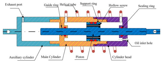
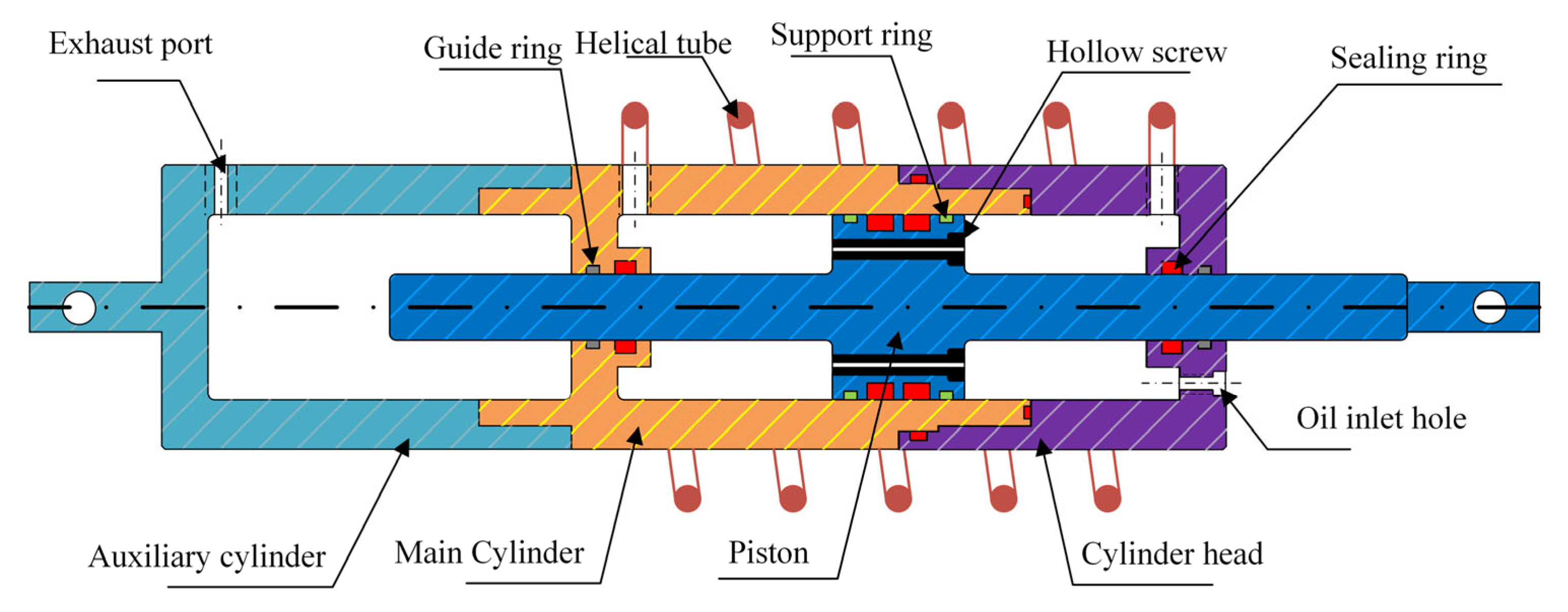
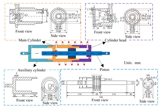
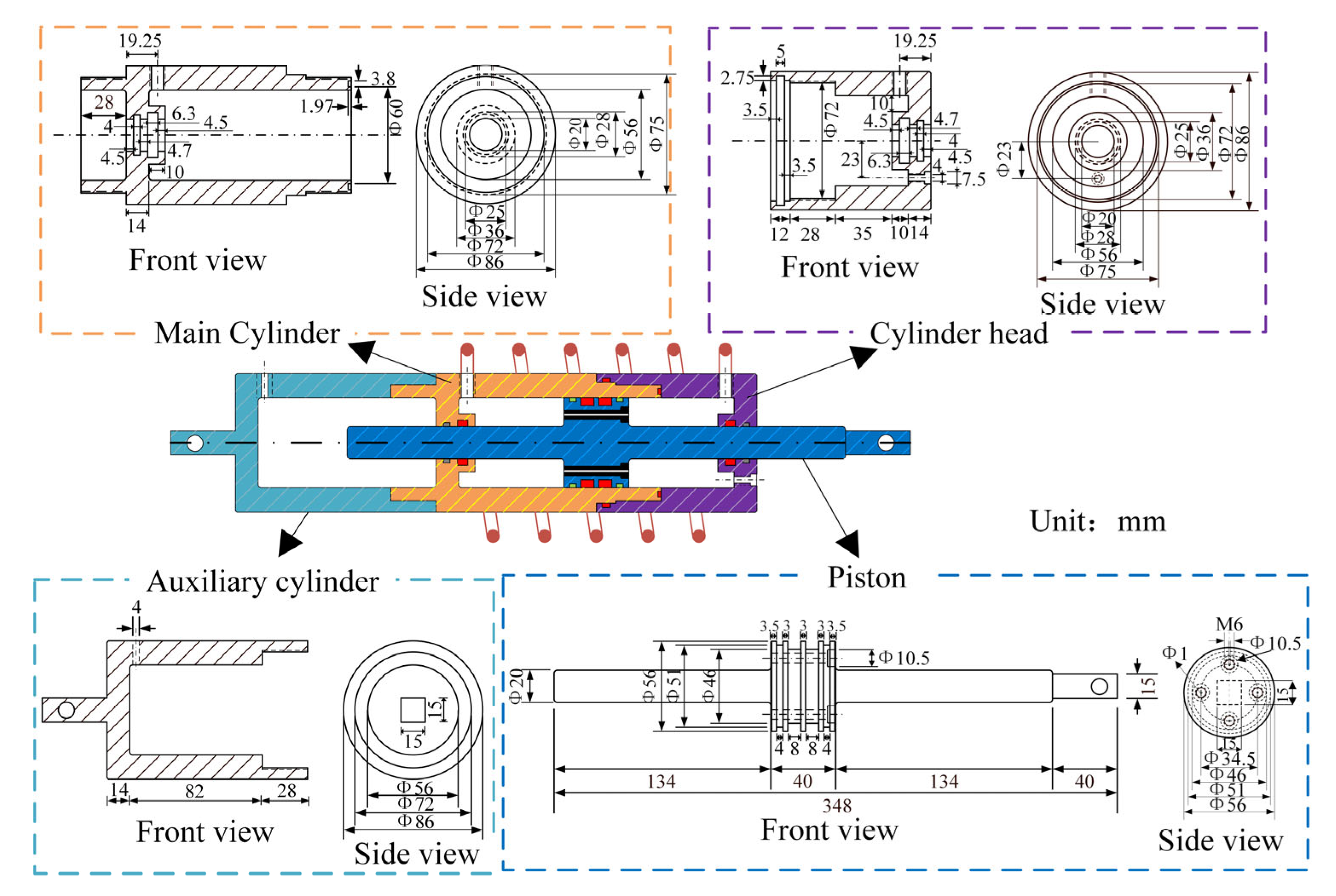
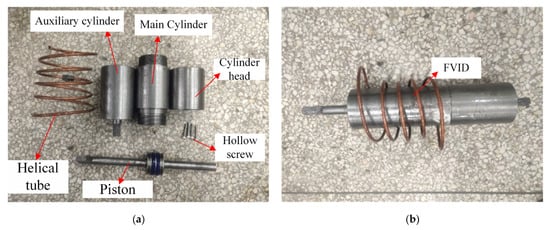
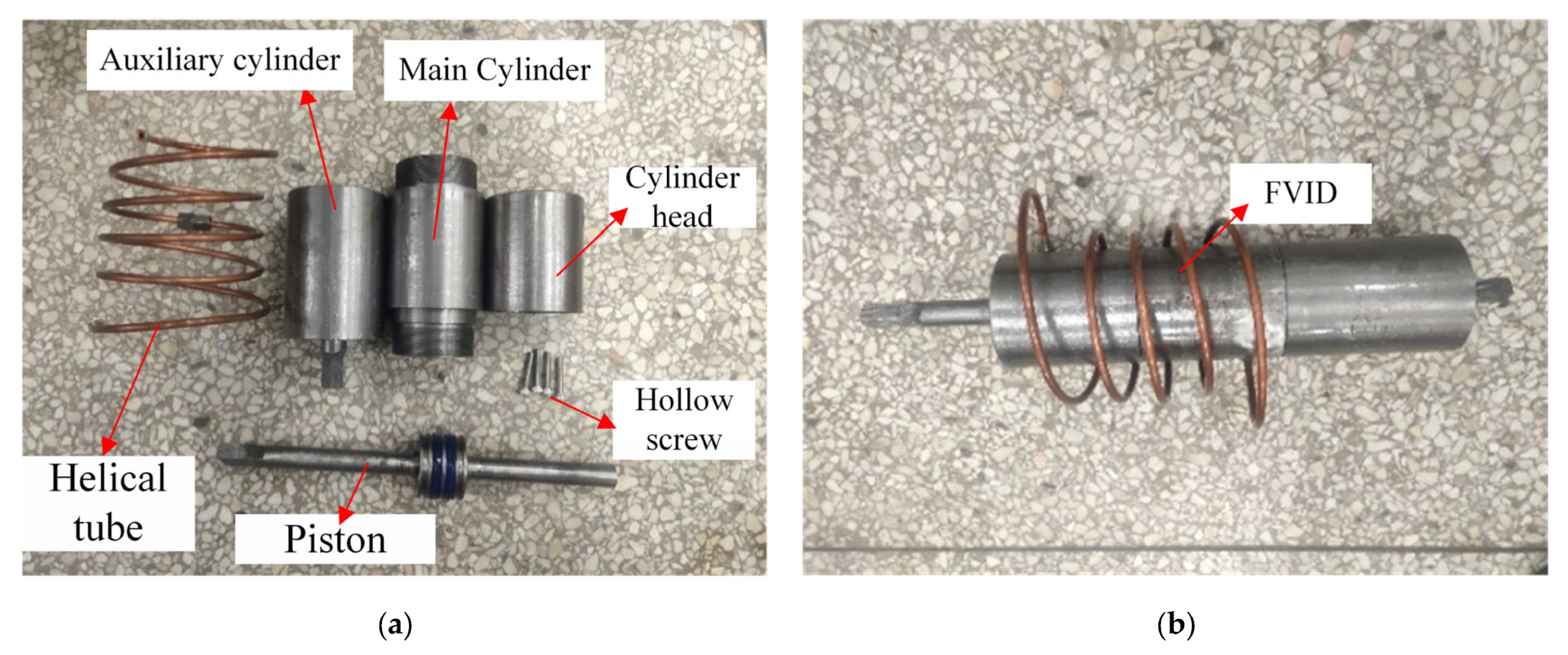
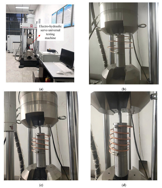
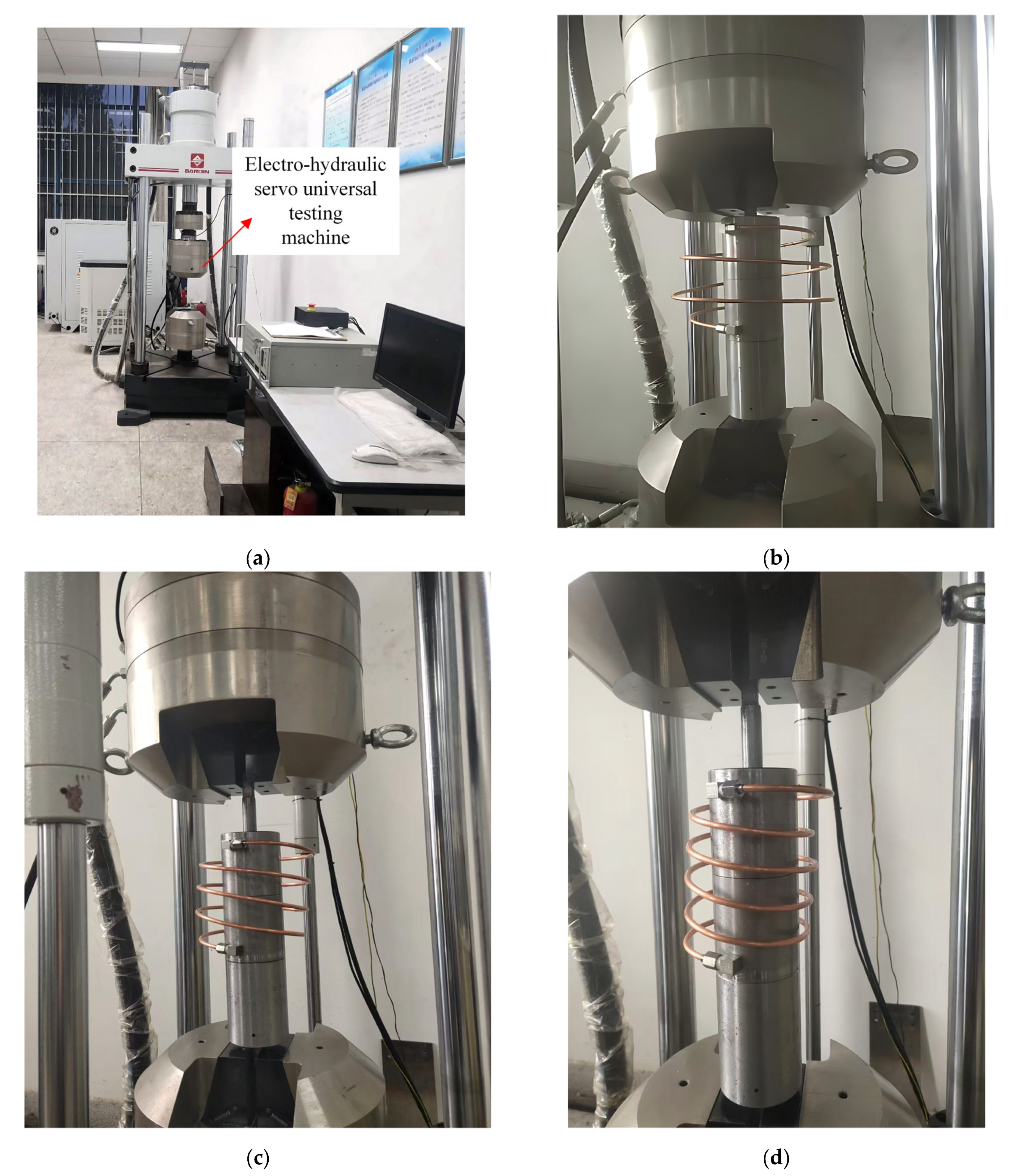
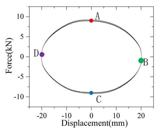
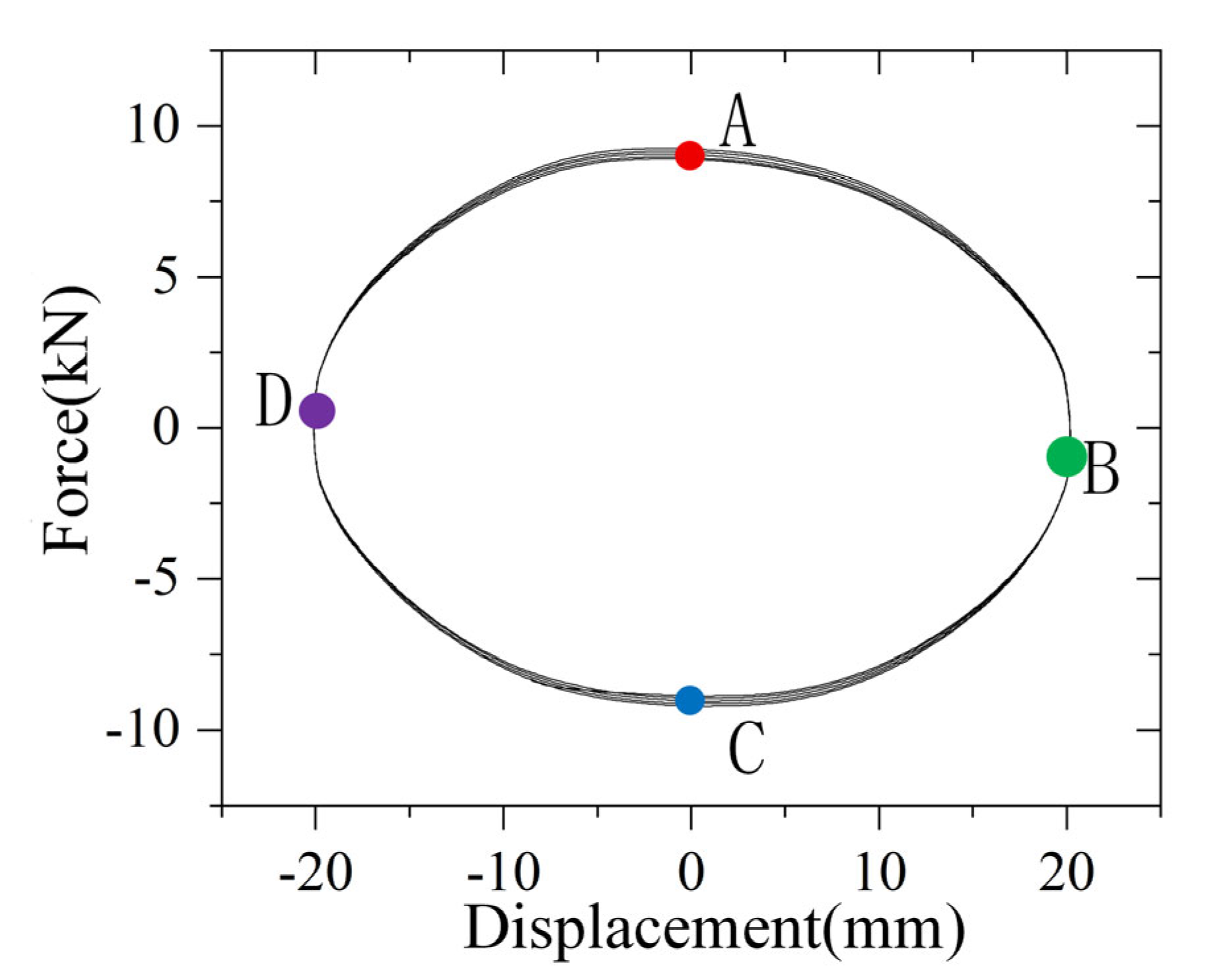
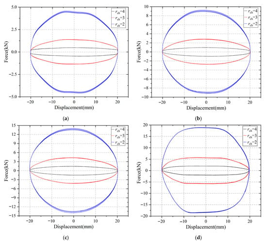
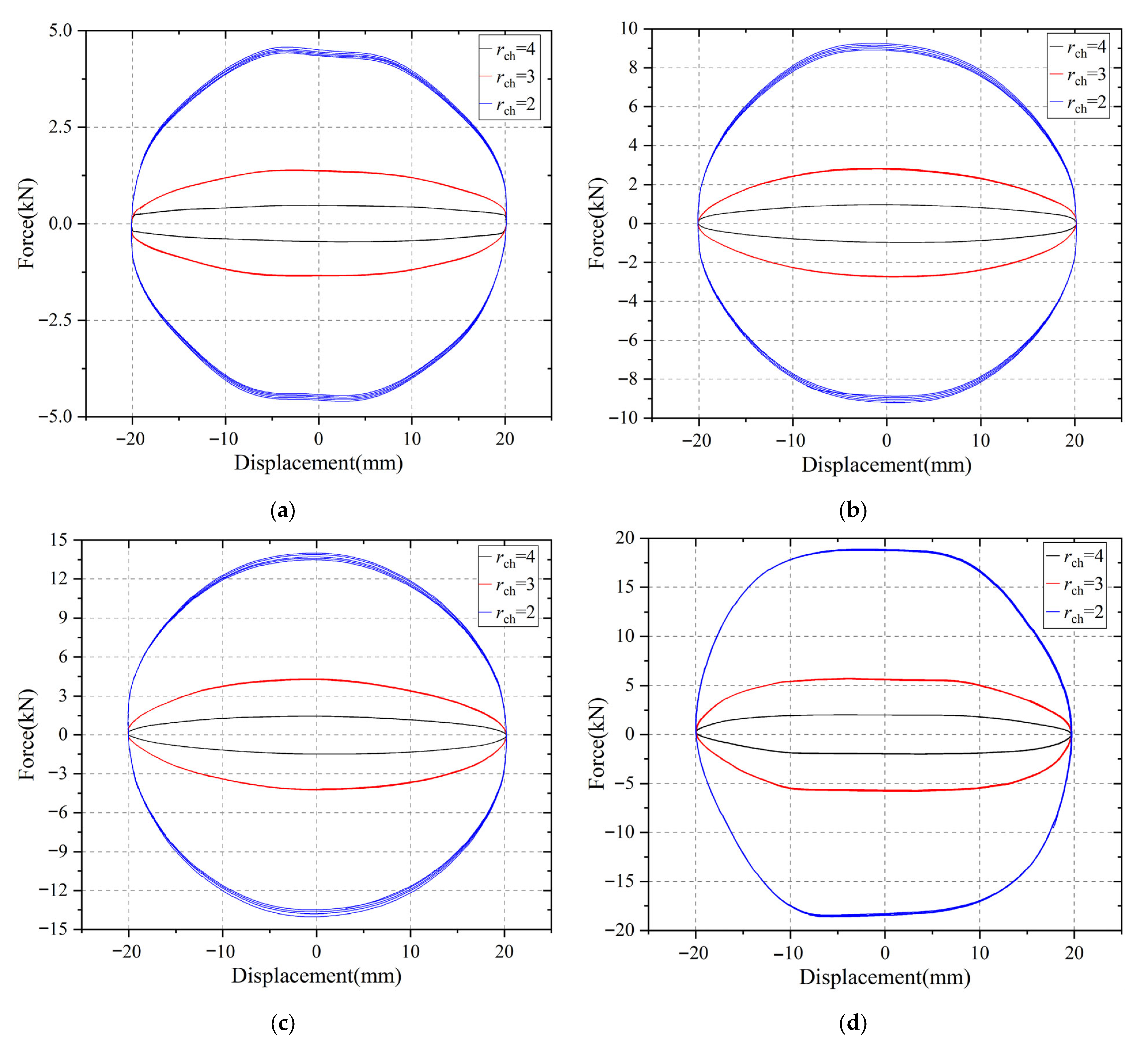
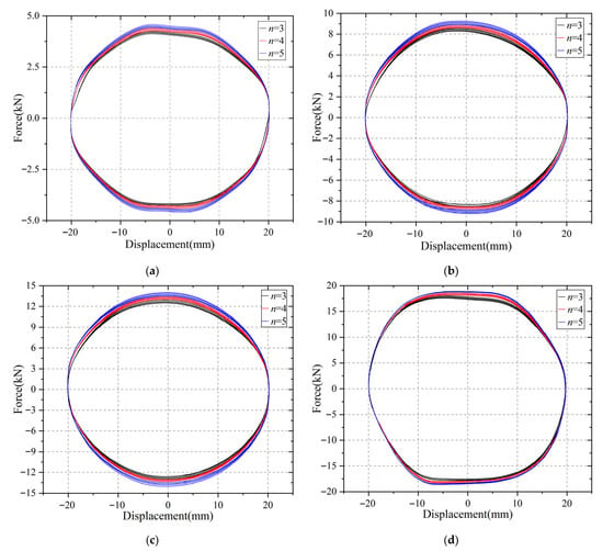
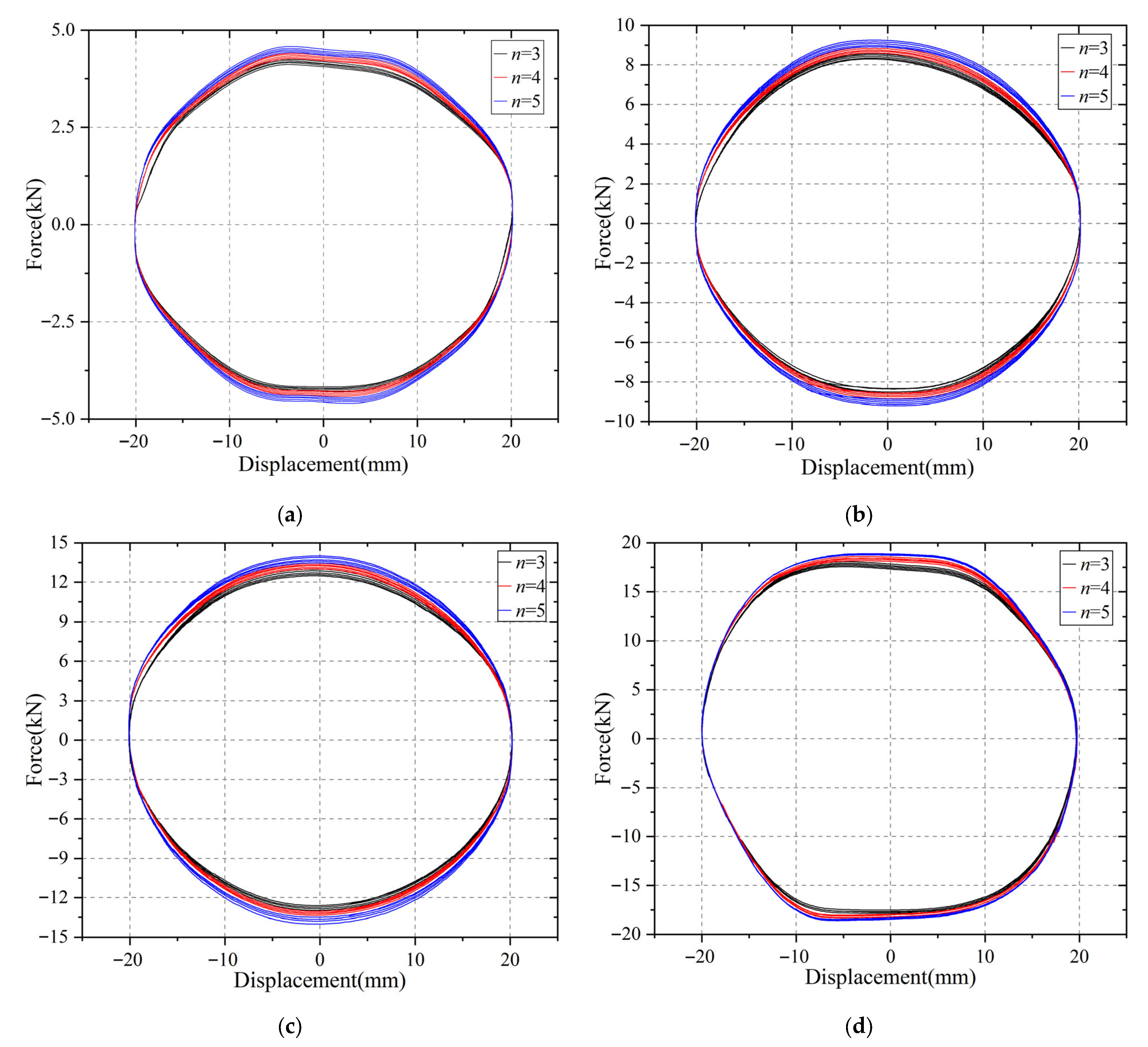
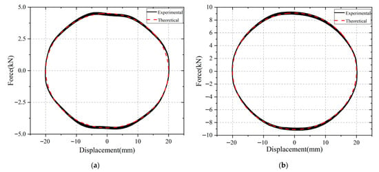
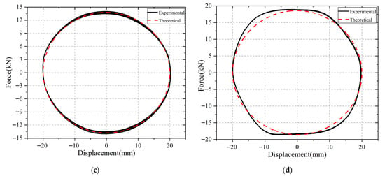
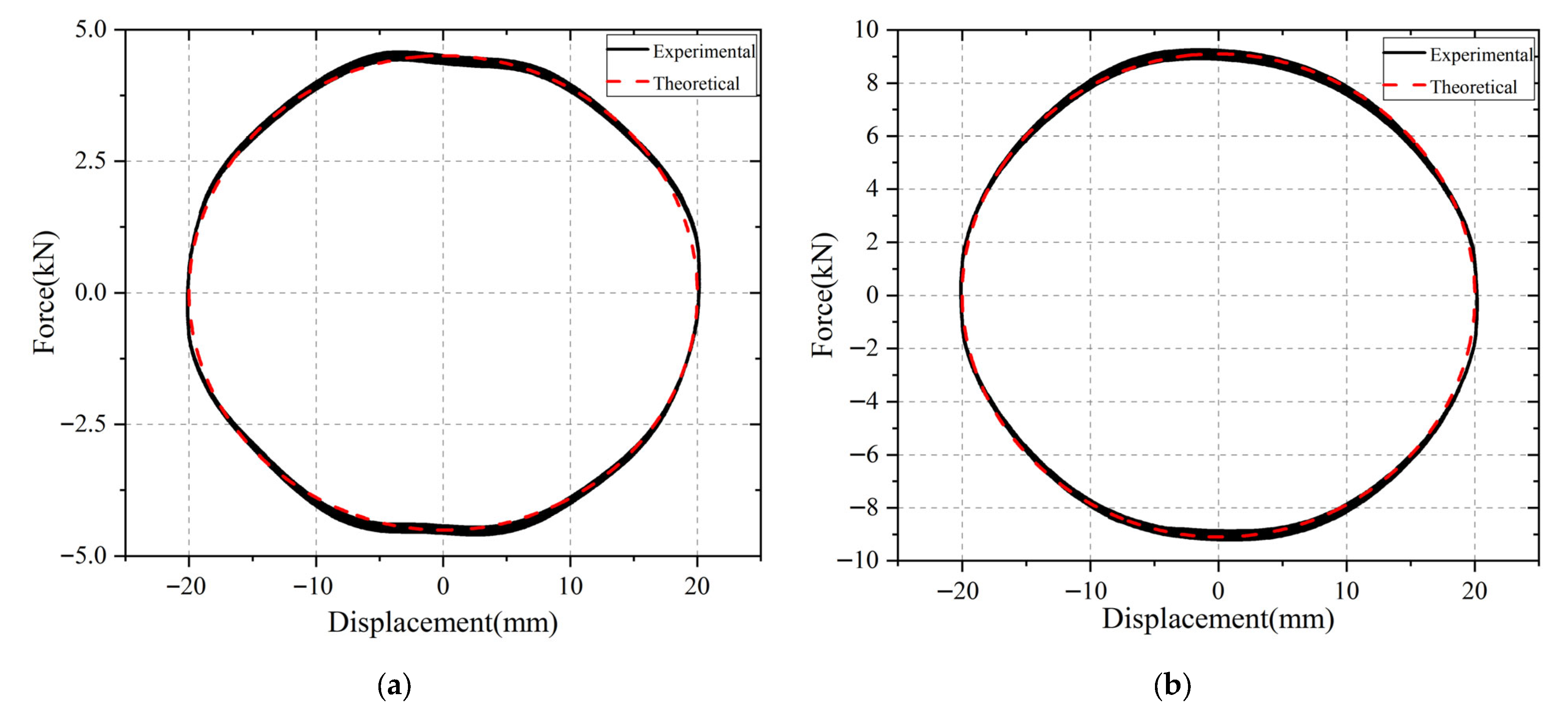
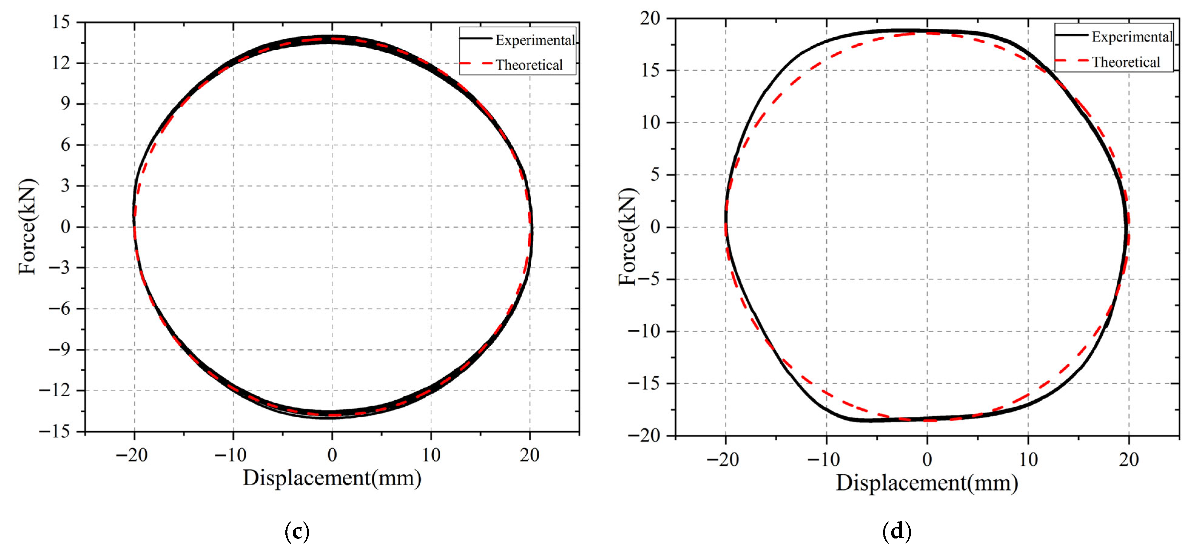
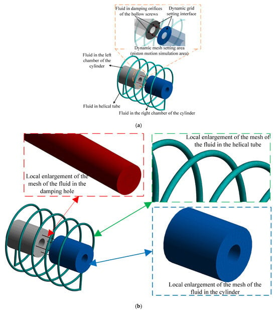
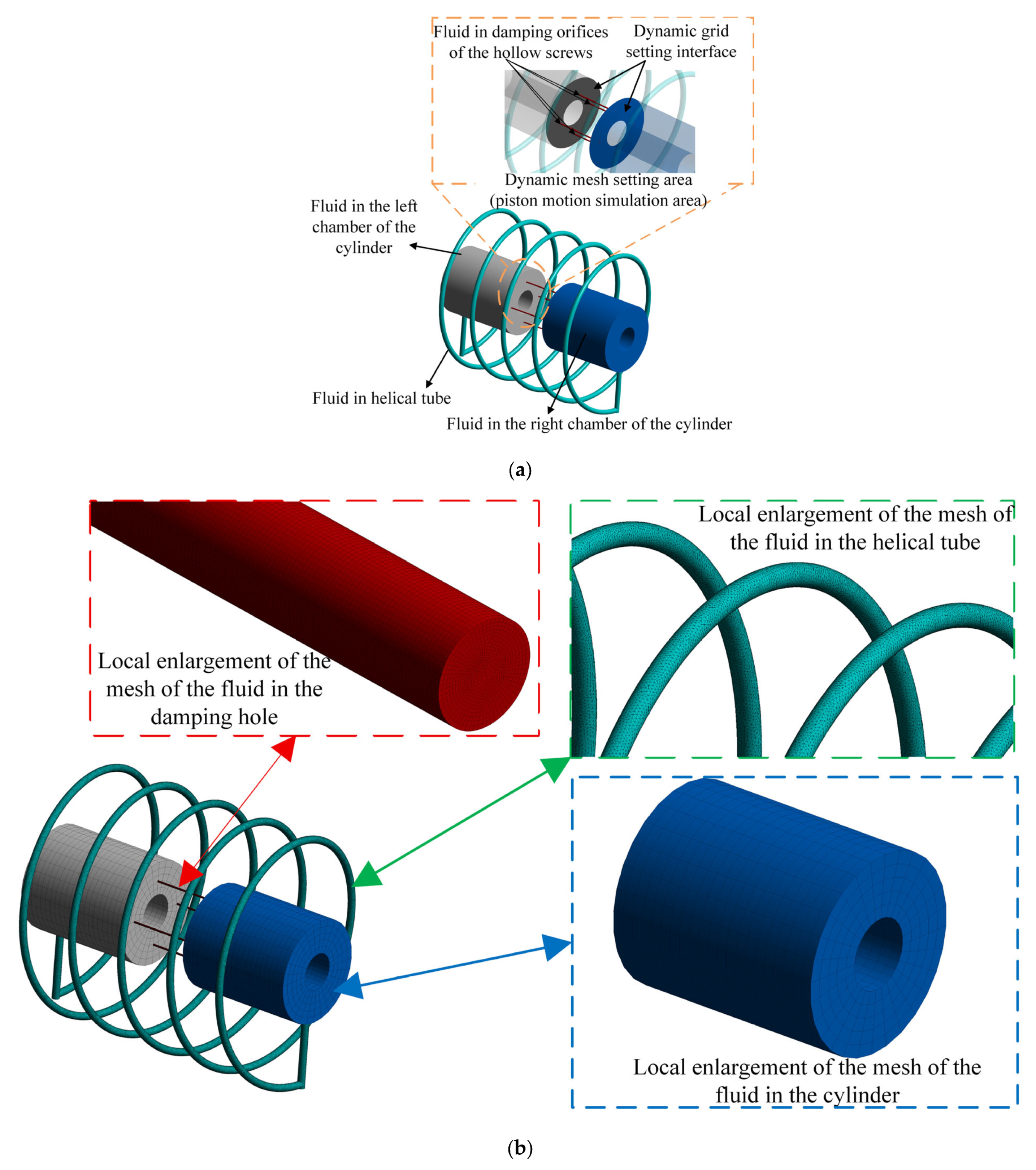
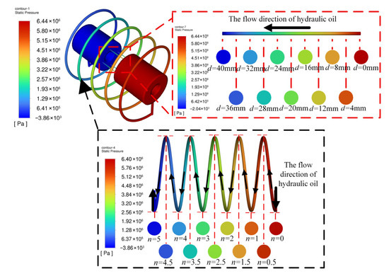
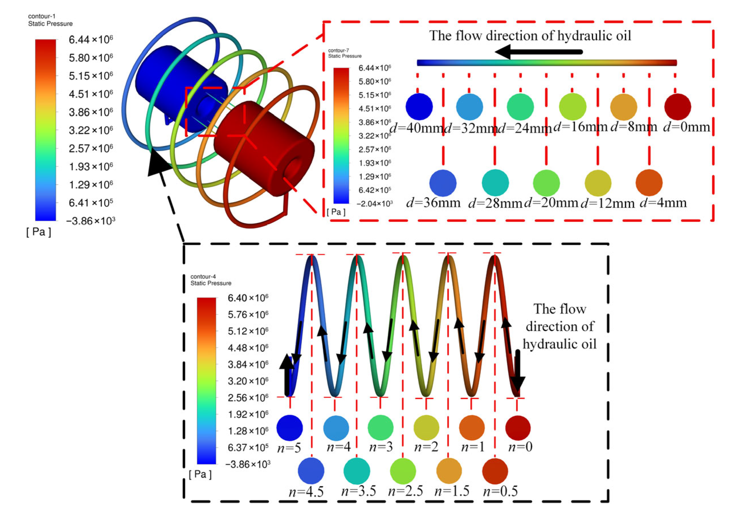
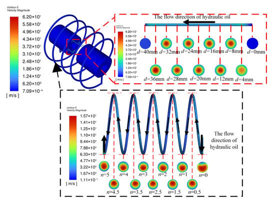
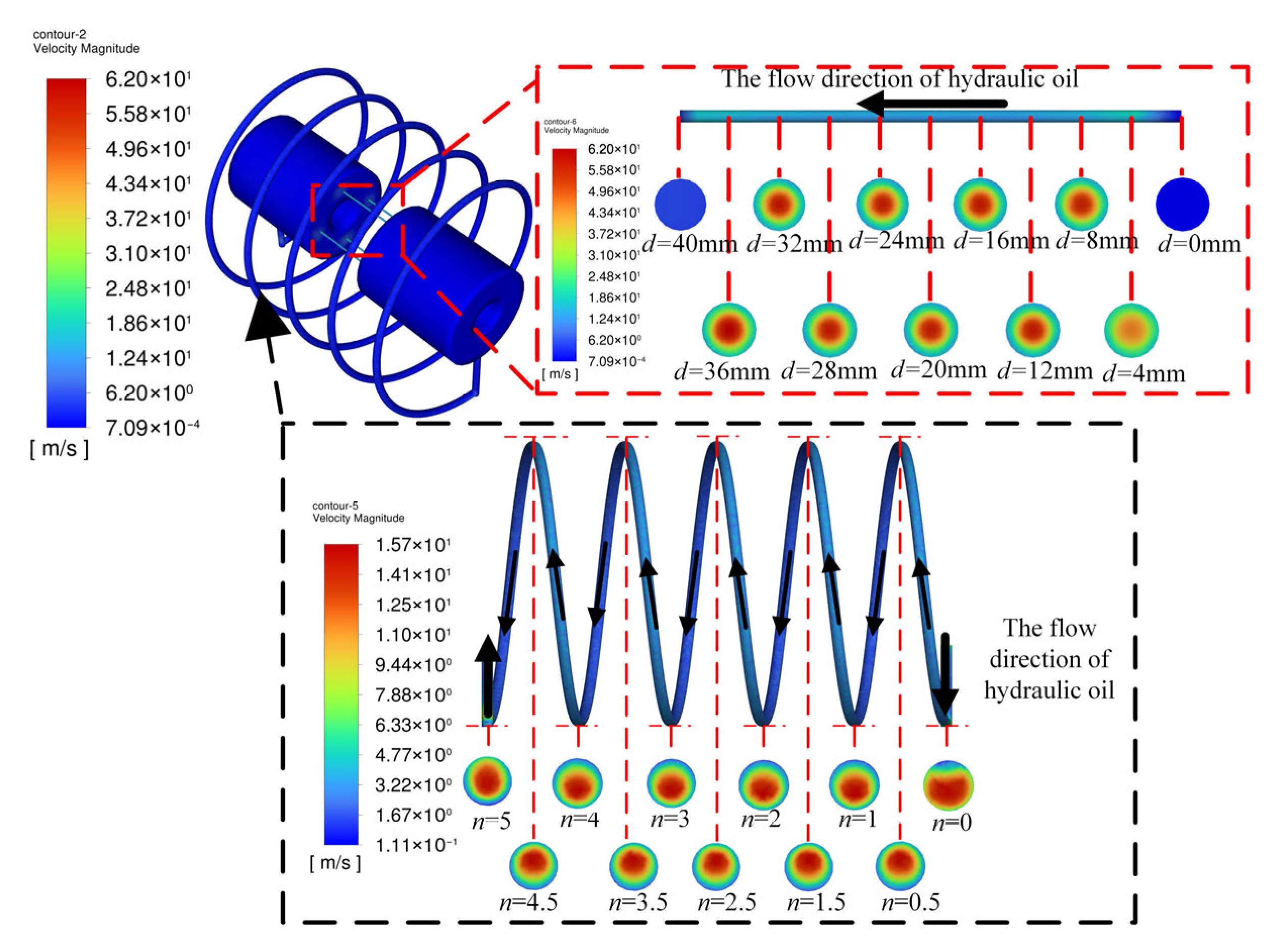
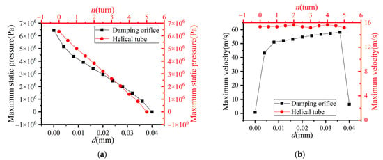
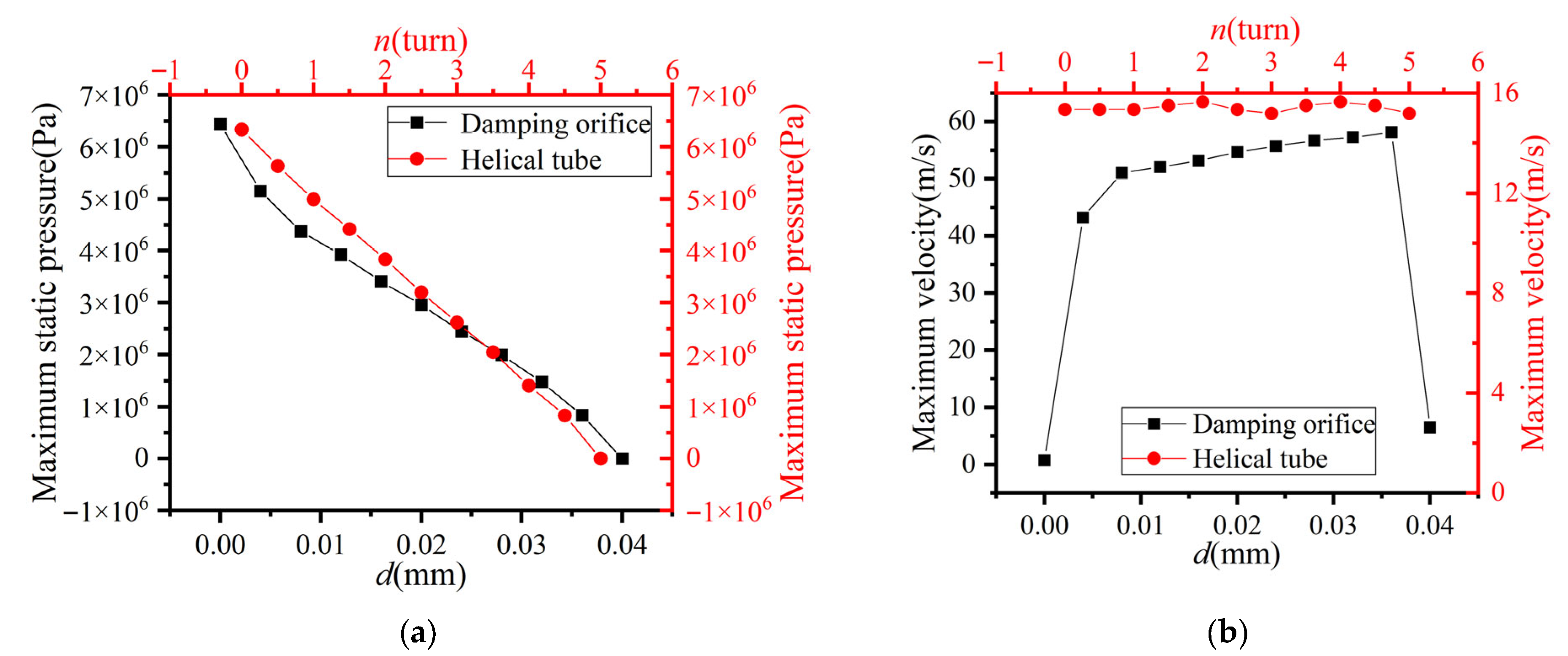
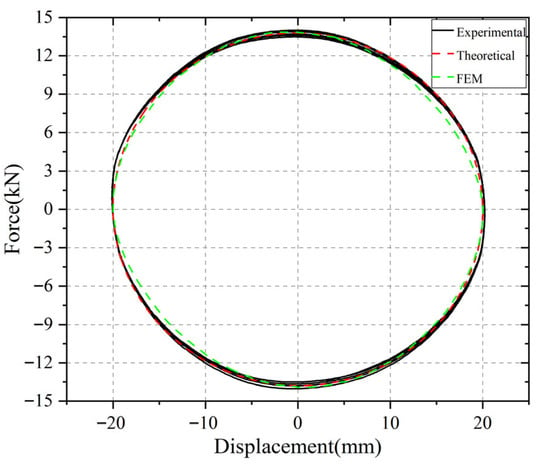
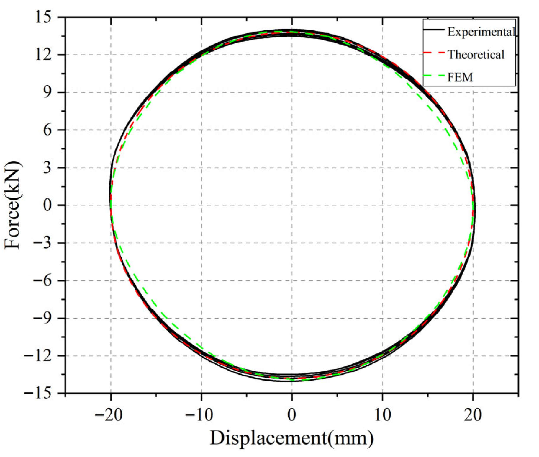
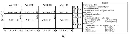
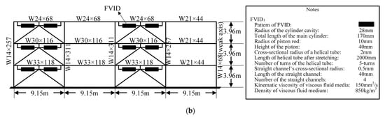
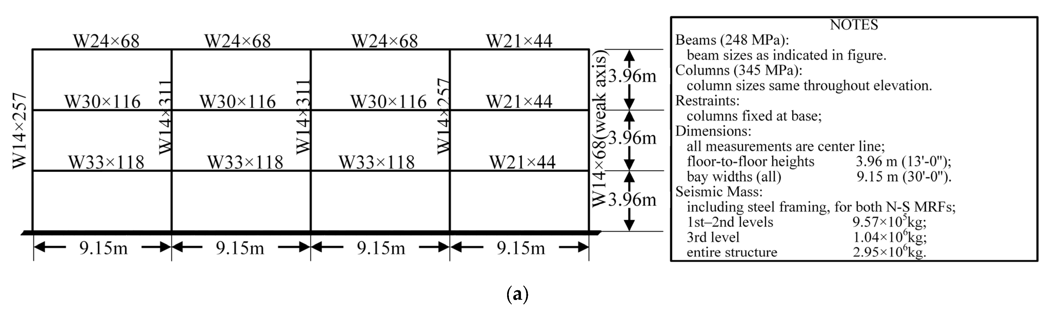
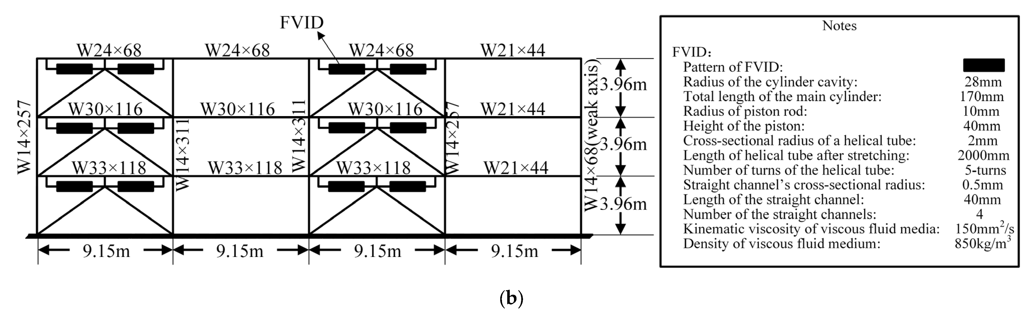
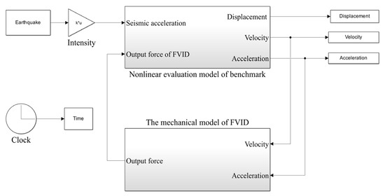
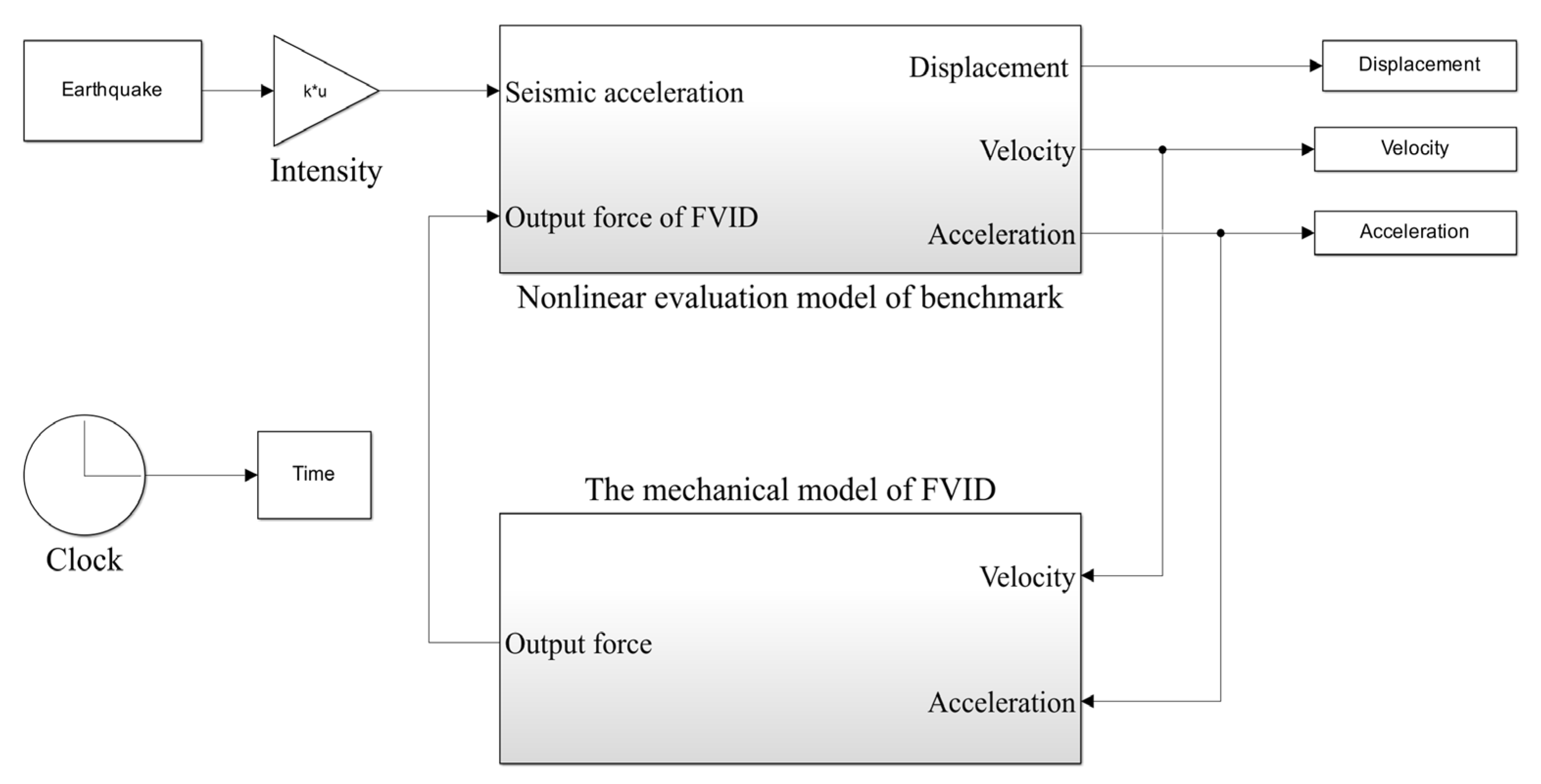
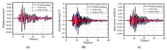
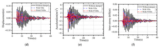
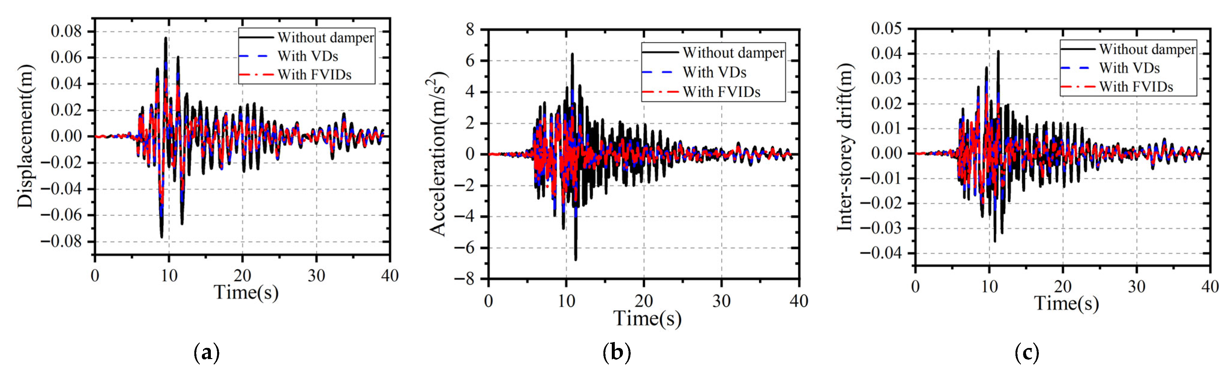
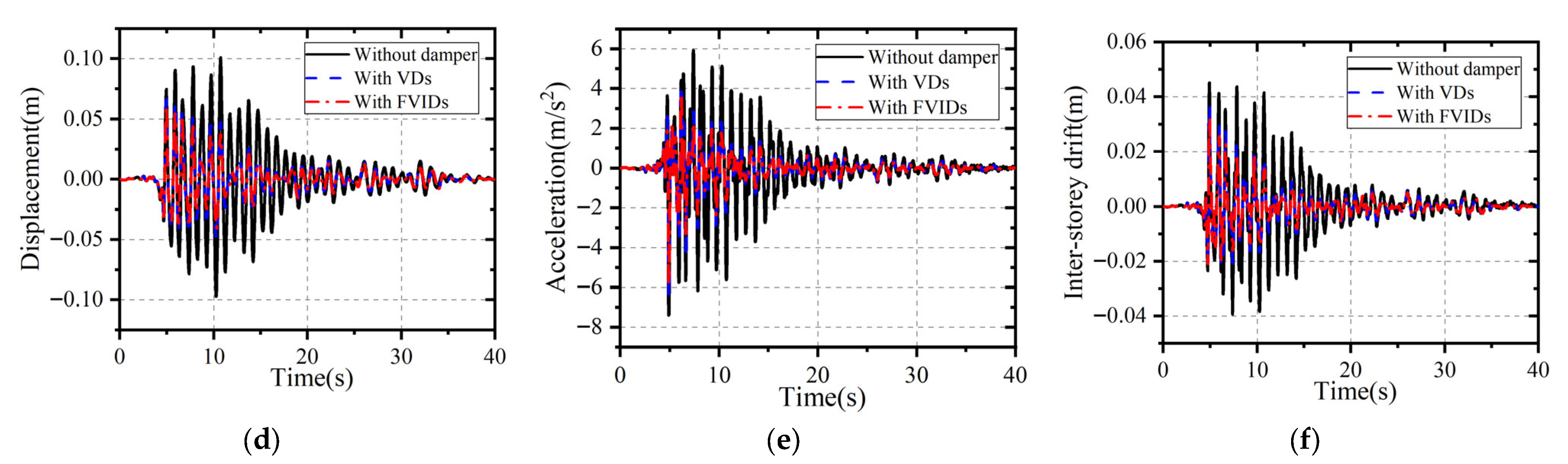
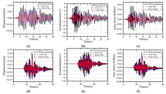
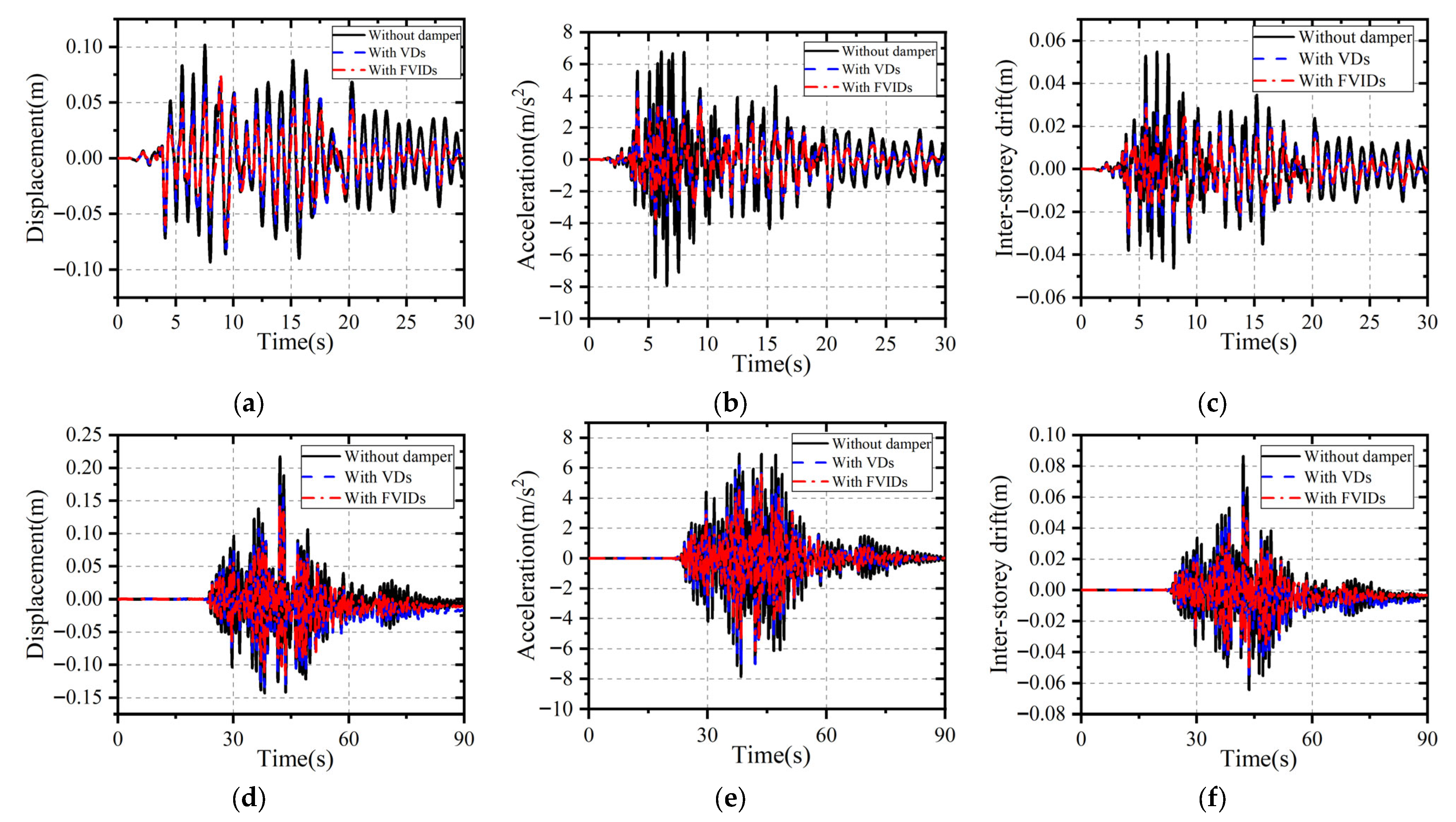
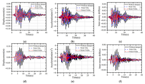
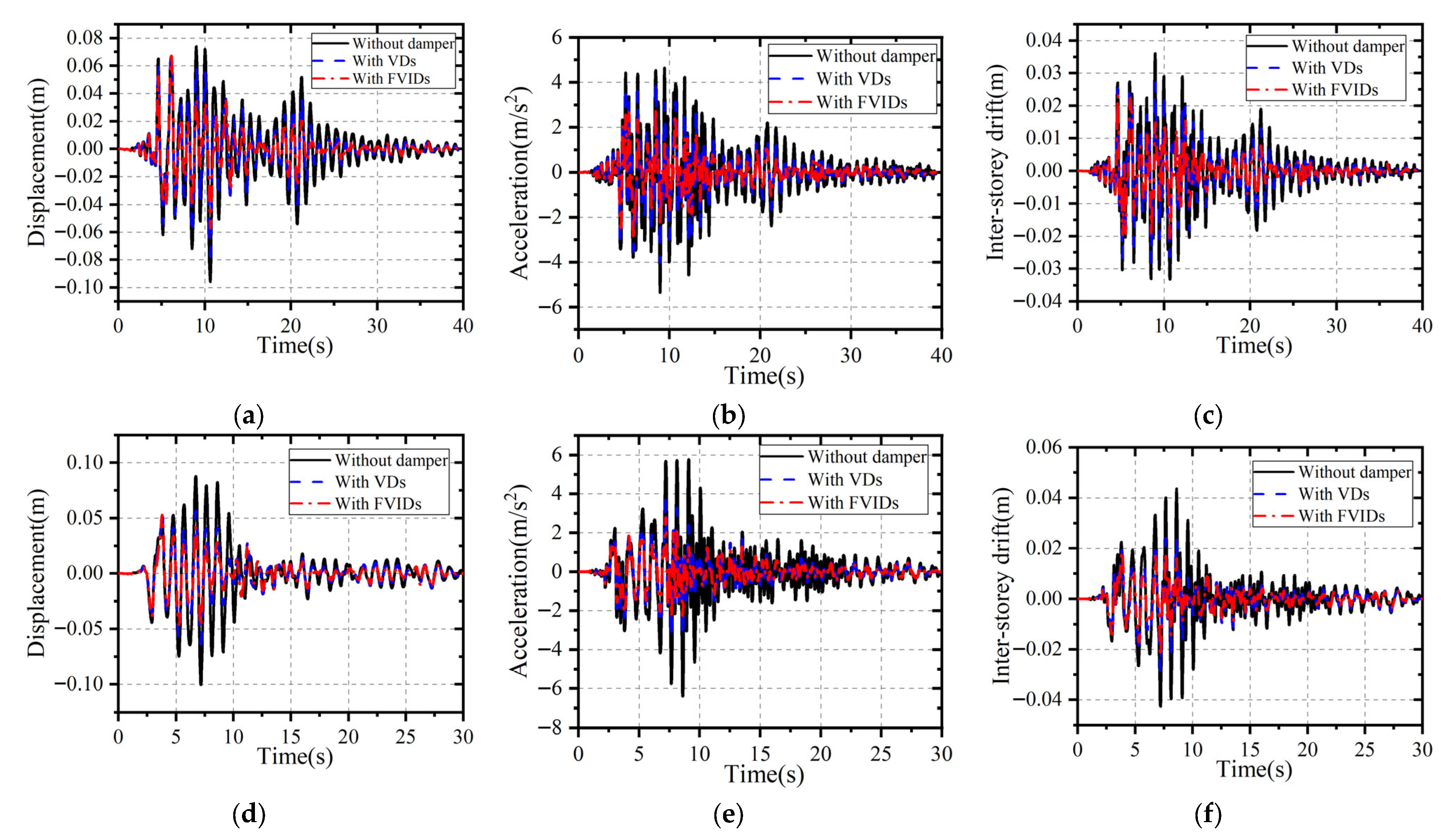

Disclaimer/Publisher’s Note: The statements, opinions and data contained in all publications are solely those of the individual author(s) and contributor(s) and not of MDPI and/or the editor(s). MDPI and/or the editor(s) disclaim responsibility for any injury to people or property resulting from any ideas, methods, instructions or products referred to in the content. |
© 2026 by the authors. Licensee MDPI, Basel, Switzerland. This article is an open access article distributed under the terms and conditions of the Creative Commons Attribution (CC BY) license.