


Abstract
Research shows that structures are often over designed in reliability-based calculations compared to code requirements. To address the knowledge gap in applying Reliability Based Design Optimisation (RBDO) within Building Information Modelling (BIM), this paper presents a novel BIM-integrated RBDO system for highway structures aimed at reducing over design. The approach is aimed at optimising the system reliability index. This value is then applied to the BIM model of the structure as a direct safety metric describing the probability of failure. In addition, minimum robustness and redundancy indices can be derived using this approach to ensure overall compliance with structural design codes, (Eurocodes), yielding key BIM model safety metrics. The system reliability index was optimised by utilising target limit state reliability indices to derive system difference target limits. System element reliability indices were effectively increased or reduced by manipulating element resistance parameters. An optimisation algorithm was employed to ensure compliance with the minimum system difference target limits. A secondary verification was undertaken to ensure minimal element target reliability indices were not compromised. The system reliability-based case studies on one-span bridge structures demonstrated that optimisation resulted in an overall 15% reduction in design resistance compared with the Eurocodes design method. In addition to highlighting element overdesign, the balance between safety and economy is improved by yielding comprehensive structural system safety metrics as a safer approach than direct element reliability-based optimisation.
1. Introduction
Evidence suggests that structural elements are commonly overdesigned by 25% to 100% beyond code requirements based on research by [1,2]. This paper outlines a novel approach using System RBDO to both improve safety and reduce costs. In addition, the framework presented also supports the golden thread principle proposed by [3]. This can be outlined as the development of a reliable, up-to-date, and easily accessible record of data for the structural design verification process that supports both the design and operational stages of the asset lifecycle.
1.1. Background
In this research, BIM is conceptualised not merely as a digital 3D representation of a structure, but as an integrated platform embodying a RBDO semantic shadow model. This strategy facilitates the systematic embedding, visualisation, and management of structural safety metrics throughout the asset lifecycle. By incorporating the system reliability index and associated robustness and redundancy indicators directly into the BIM environment. The BIM model evolves into a continuous, traceable source of truth that supports decision-making from design through to operation and maintenance. This integration enables stakeholders to assess and verify structural performance in real-time. This approach ensures compliance with design codes and enhances transparency, resilience, and safety in infrastructure management.
Structural System RBDO refers to the optimisation of elements in a structural system to ensure there is an adequate probability of performing its intended function for a specified duration under defined conditions. Refs. [4,5] suggested that structural reliability is essentially a rational framework that provides a quantitative measure of uncertainty. Ref. [6] suggested that the probability of failure and reliability index are key measures for quantifying the safety of a structural system based on uncertainties relating to load effects, element resistance, and modelling parameters. Ref. [7] proposed that the reliability index and probability of failure were essential metrics for the transition from deterministic to probabilistic safety factors in risk-based design. Ref. [8] stated that the probability of failure and reliability index were two sides of the same coin, reflecting the uncertainty relating to load effects and element resistance. Ref. [9] outlined that the reliability index and probability of failure were practical metrics which quantified structural safety in terms of probabilistic rather than deterministic design.
This paper forms part of a broader research strategy, as shown in Figure 1, and proposes a novel approach for integrating System RBDO into a BIM integrated bridge design framework.
Figure 1.
BIM-Based Whole Life Asset Management Approach: a probabilistic design and maintenance methodology for quantifying risk of structural failure.
1.2. Specific Research Problem (Literature Review)
Most structural design codes, including BS EN 1990 [10,11] and ISO 2394 [12], adopt the ‘weakest link’ approach to structural system reliability [13]. Under this approach, the structural element with the lowest reliability index or highest probability of failure is assumed to represent the reliability index or probability of failure of the entire structure. The ‘weakest link’ approach is commonly used because numerically solving the system correlation coefficient using multifold integrals is difficult [14]. The weakest link approach enables structural design codes to largely overlook structural system reliability by requiring only a very low target probability of failure for individual elements (BS EN 1990 [4,10,11]). However, this can be counterproductive and potentially unsafe, particularly in structural systems composed of multiple elements or subsystems acting in series.
RBDO has evolved over several decades into a well-established discipline within engineering. The main challenges with RBDO arise from the unknown parameters such as the specific Probability Density Function (PDF), covariance, and statistical model factors [15]. Moreover, existing RBDO methods are often highly mathematical and typically require multiple iterations to obtain an accurate solution [16]. Due to the complexity of generating characteristic load and action effects from first principles, which generally require site-specific continuous probability distributions modelled via finite element or rolling load analysis, action effects were derived deterministically or calculated based on structural codes and then used as a safe approach. Action effects remain anchored except for the application of mean factors and covariance parameters, which are derived from standard reference models via secondary research.
Ref. [16] identified a major issue with RBDO: the number of constraints often leads to nested optimisation problems, (optimisation problems within an optimisation problem). Therefore, the approach recommended is to concentrate on only the most important constraints and ignore lesser constraints. Based on sensitivity testing, one of the most onerous constraints is that of combined modal failure. Previous studies by [17,18,19] have generally utilised nested optimisation loops, separating design and reliability analysis, which require resource-hungry finite element or Monte Carlo simulations. The drawbacks of these approaches are as follows.
- Problem and or failure mode definitions may neglect whole system failure.
- Model complexity and potential error rise proportionally to the number of parameters.
- Focus on constraints rather than optimisation.
- Optimal solution failure due to issues with convergence for nonlinear functions.
RBDO is often neglected in mainstream practice. This is due to a combination of factors, including professional liability concerns, unfamiliarity with the method, mathematical complexity, lack of standardised reference model information, and the time required to run computer simulations to obtain realistic solutions [15].
This paper proposes a novel approach that utilises a series of single-loop linear optimisations to determine the optimal element resistance within a system, based on a specified target reliability index. The proposed system-level RBDO framework employs a three-stage process, as outlined below, to reduce computational complexity and alleviate the computational burden. This structure is considered suitable for scaling to Building Information Modelling (BIM) environments.
1.3. Objectives/Research Questions
The objectives of this research can be stated as follows.
- To reduce the over design of structural elements and improve structural system safety metrics. Essentially, we sought to develop a framework or system to improve the balance between safety and economy in structural design.
- Explore the differences relating to element and system RBDO to assess the safest approach.
- Development of a viable safe system Reliability-Based Design Optimisation (RBDO) framework which could integrate into a Building Information Modelling (BIM) platform using standardised sets of equations and algorithms.
1.4. Roadmap/Structure of Paper
Most current studies in the field of RBDO are concerned with novel multivariate techniques aimed at optimising the design parameters of one element in one mode of failure. Typically, Rosenblatt Transformation or similar techniques [20,21] are utilised for multivariate element RBDO. Due to the sophistication of modern methods of structural analysis and design, multivariate methods of reliability analysis have been discounted when considering BIM models due to the following issues.
- Complexity of developing limit state equations from first principles. Nonlinear limit state equations often require extensive use of partial differential calculus to develop a complex solution, which does not fit with the aim of developing a standardised algorithm for use in BIM models.
- The difficulty of identifying the multitude and prioritisation of competing constraints and how these are modelled.
- The time and resources required to develop viable solutions to explore all reasonable multi-modal failure probabilities.
- Ref. [22] suggested that multiple variables increase the presence of uncertainties in practical engineering problems significantly. Minimising the number of variables reduces uncertainty and errors, generating more confidence in the result. Linear bivariate analysis will generally be simpler to achieve and less prone to error than nonlinear multivariate analysis.
Ref. [23] suggested “to analyse an engineering problem, you need to simplify it until you can solve it: all simulation is simplification”.
1.4.1. Stage (1) Multimethod Confidence Limit Linear Element RBDO
Based on the above limitations and the need to efficiently and effectively develop modal failure probabilities for flexure, shear, axial compression, and/or tension of a structural system, a multimethod approach incorporating two linear optimisation bivariate approaches as described below has been adapted to yield upper and lower bound statistical safety limits for element resistance for a given mode of failure. The two variables forming the bivariate approach are load effect and element resistance. The optimisation methodology is to anchor the load effect to generate the optimal element resistance based on a target reliability for each mode of failure utilising standard reference models.
This approach therefore allows for the development of standardised equations and algorithms to be utilised by the BIM model. It avoids the layers of complexity generated by multivariate non-linear analysis when considering a multimodal failure of a structural element.
First Order Reliability Method (FORM)
The FORM is proposed based on using anchored Load Effects (E) deterministically derived from codes and theoretical analysis and Element Resistance (R) derived from a target reliability index. This approach has the following advantages.
- The number of constraints is minimised for the optimisation problem.
- A linear limit state equation is generated, so local optimums are negated in the optimisation solution.
- The number of variables and assumed probability parameters is minimised, indirectly reducing potentially large errors.
- The need to resort to high level mathematics of partial differential calculus is negated.
- Standard equations are generated for each mode of failure, including flexure, shear, axial compression, and tension for the optimisation.
- Based on standard reference models, load effects and element resistances are modelled via either the normal or log normal probability distribution, negating the need for more inordinate distributions. This allows the failure probability to be derived from the reliability index using the standard normal distribution.
The normal probability distribution (see Figure 2) was developed by [24] as a method of rationalising the least squares method for optimisation problems. The normal probability density function is used to maximise the probability of estimating an unknown parameter and is the foundation of several reliability optimisation methods.
Figure 2.
Standard Normal Distribution Bell Curve, Standard Deviation (σ) & Mean (μ). (Adapted from [24]).
Centile Design Point Method (CDPM)
The method essentially takes a quality control approach to structural reliability utilising an Upper Control Limit (UCL) for Load Effects known as (Ed), typically ranging over 95% of the maximum possible load effect value. The Lower Control Limit (LCL) for Element Resistance (Rd) typically ranges less than 5% of the maximum possible design resistance. Standardised algorithms generate the reliability index (β) utilising FORM Factors αE and αR, (Load Effect and Element Resistance, respectively) in combination with the mean values. The LCL and UCL are developed in terms of percentiles of respective probability distributions. Typically, standard normal or log normal probability distribution functions are commonly used for this method, see Figure 2.
The multimethod approach adopted in this research essentially manipulates the accepted FORM and Centile (CDPM) methods by utilising a target reliability index. In this way, it develops estimates of element resistance and reliability indices within confidence limits using a standard library of reference models.
A safe (conservative) approach has been applied: the lower confidence limit is used for estimating the element reliability index, as this represents the highest probability of failure. Similarly, the upper confidence limit is used for the element’s mean resistance, since this produces the lowest probability of failure, (see Figure 3 and Figure 4 below).
Figure 3.
Estimated reliability index over time, adopting the safe approach of using the highest probability of failure or lower confidence limit.
Figure 4.
Estimated mean element resistance over time, adopting the safe approach of using the lowest probability of failure or upper confidence limit.
Since System RBDO relies primarily on the calculation of element failure probabilities, Figure 5 has been included to provide a general outline of how element failure probabilities can be derived and incorporated into a BIM integrated framework. Figure 5 shows that element design can be derived by either a probabilistic or deterministic approach.
Figure 5.
BIM Based Element Resistance Design Approach using probabilistic or deterministic methods.
The element reliability indices can then be incorporated into the System RBDO framework. Load effects such as compression, flexure, or shear are obtained deterministically using design codes and structural analysis. These load effects remain anchored, apart from mean factors and covariance parameters derived from standard reference models, which simulate the relevant probability density function. According to Refs. [13,16], the element RBDO process seeks to determine the element resistance using probability algorithms. Target reliability indices specified in BS EN 1990 [10,11] or ISO 2934 [12] can be used to achieve a minimum probability of element failure under stochastic actions or load effects.
1.4.2. Stage (2) Combined Modal Element RBDO
Optimising any single failure mode is often significantly constrained by the combined effects of multiple failure modes, where interactions between modes can reduce the resistance of a structural element in another mode. The Eurocodes outline the combined failure modes that must be considered, which typically include combinations of flexure or bending, shear, and axial compression (see Figure 6 below). The important constraint is that optimising resistances for individual failure modes such as flexure, shear, or axial compression and tension can reduce the combined modal reliability index below the target safety level, potentially leading to design failure of the structural element.
Figure 6.
Typical Union of Modal Failures (Combined Effects).
1.4.3. Stage (3) System RBDO
The optimised element metrics can be stored within the BIM model and subsequently extracted for use in System RBDO, as illustrated in Figure 7. The key properties of a system typology that have an influence on the system’s probability of failure can be outlined as follows:
Figure 7.
BIM-Based System Reliability Based Design Optimisation using probabilistic methods to determine robustness, redundancy and structural safety indices for structural design. The key system limit states are described later in this paper.
- Structural System element correlation
- Structural System Reliability Index (Safety Index)
- Structural System robustness
- Structural System redundancy
The system parameters are ignored by a purely elemental approach [25,26]. This research therefore aims to address this issue by developing an effective and integrated approach to BIM modelling of structural systems, enabling the evaluation and optimisation of system topology during the design stage to ensure minimal system safety, robustness and redundancy metrics can be achieved.
The approach employs structural design on the effects of applied loads on member strengths, and the reliability evaluation in the context of structural system optimisation and safety analysis. The approach optimises the system’s reliability while deriving robustness and redundancy indices, integrating safety metrics and code compliance. The System RBDO approach incorporates three stages of a nested optimisation as follows.
Stage (1) Multimethod Confidence Limit Linear Element RBDO, which uses statistical confidence limits to yield a safe upper bound element resistance and lower bound reliability index or probability of failure.
Stage (2) Combined Modal Element RBDO utilises a weighted gradient optimisation to yield each minimum modal resistance to satisfy the combined element target resistance.
Stage (3) System RBDO, which also utilises a weighted gradient optimisation algorithm, is employed to adjust element resistances to meet target system reliability indices, with secondary verification to maintain minimum element safety.
Case studies on one-span bridges are used to demonstrate that system level RBDO can reduce design resistance while enhancing overall structural safety, addressing the gap in integrating system reliability metrics into BIM for informed, lifecycle-aware structural design. The criteria used for evaluation will be a comparison between traditional design, element RBDO, and the proposed novel system RBDO approach.
2. Materials and Methods (System Development)
2.1. Background to Structural Reliability
The general method of obtaining the structural failure probability is summarised in Figure 8, which shows the idealised worst case probability density functions for both the load action effect and resistance assuming worst case skews (positive for action load effect and negative for resistance). The shaded area of Figure 8 shows the risk zone of potential failure. The Gumbel, Weibull, and other probability distributions can be included to accommodate extreme load effect values such as earthquakes, winds, snows, and flooding [27]. Generally, these inordinate distributions are not suitable for load effect or element resistance estimation. Extreme load effects are captured in the deterministic design code approaches, so inordinate probability distributions are negated. There is a limit placed on the lognormal distribution covariance value of <0.2 in BS EN 1990 [10,11], as higher values of covariance yield potentially unrealistic theoretical models where the probability of error increases. This is due to the relationship between covariance and the skewness of the lognormal probability distribution as suggested by [13], who suggests that in practice it is common to use a covariance value below 0.4 for lognormal PDFs, although caution and judgement should be used. To estimate the reliability index (β), the Limit State probability density function is developed in Figure 9.
Figure 8.
Probability Distribution Functions of Resistance (R) & Load Effect (E), (Adapted from [13]).
Figure 9.
Limit State Probability Density Function, (Adapted from [4]).
The failure probability (see Figure 9) can be expressed as follows based on [4].
where Pf is the probability of failure, R is Element Resistance, E is Load Effect, and x is a specific or discrete random independent value. This yields the general reliability integral, but the probability distribution is unknown, where x may take any value between +/− infinity (ꝏ) [4].
To simplify the problem of continuous probability distributions and avoid the confusion of mixing different probability distributions, the standard normal probability distribution is utilised by most structural codes like BS EN 1990 [10,11] and ISO 2394 [12]. This is a pragmatic approach, as other probability distributions can be readily transformed into the normal distribution. Ref. [25] solved the invariance problem by transforming the limit state function into standard space. (See Figure 10 and Figure 11).
Figure 10.
3D—Transformed Limit State Function into Standard Space, (Adapted from [4]).
Figure 11.
2D Plan—Transformed Limit State Function into Standard Space, (Adapted from BS EN 1990 [4,10]).
The approach adopted by Ref. [25] seems to have been derived from the probability method of the difference between two means for bivariate analysis developed by [28]. This approach is widely applied in various optimisation algorithms to estimate unknown parameters using Gaussian probability distributions, with applications spanning medicine, economics, financial markets, and multiple engineering domains. Furthermore, the method can be adapted through the Rosenblatt Transformation for multivariate analysis, as demonstrated in the author’s research.
The reliability index β is the shortest distance between the centre of the joint PDF (µR, µE) means of Resistance and Load Effect to design point (r*, e*) at the apex of the failure surface of the joint PDF, as outlined in Figure 10 and Figure 11.
Hence, the Reliability Index β is obtained as the solution to a constrained optimisation problem in a standard normal space.
Several methods or algorithms can be used to solve the above optimisation problem, including gradient, projection, Lagrange, and reduced gradient methods. However, the [25] method is commonly used due to its simplicity and was extended by [26] to accommodate random variable distribution information. By manipulating the standard normal distribution equations, ref. [29] derived an expression for the reliability index (β) in terms of failure probability Φ(-β). This reliability index is based on the Gaussian or Standard Normal Probability Density Function (PDF) as follows.
where Pi is the element or system probability of failure. β is the element or system reliability index. Φ is the cumulative Gaussian PDF.
Based on the FORM approach used by [25], the following equations were derived to estimate the probability of failure in terms of the reliability index (β).
where
- and
2.2. System Development
Based on [13], Table 1 shows that when different RBDO methods are compared, the variation in the reliability index is generally minimal, except for statistical outliers. The variation between the maximum and minimum probability of failure is nearly a factor of ten, leading to the upper reliability index estimate potentially being unsafe. To counter this the lowest confidence interval value of the reliability index is adopted to yield a safe but reasonable approach. By assessing multiple RBDO methods for the same problem, it is possible to limit variance by using a statistical standard error approach to develop an upper and lower confidence interval. By using the lower reliability index confidence interval, the highest probability of failure is obtained, which is deemed a safe approach as presented above. In a similar manner, by manipulating the Structural Reliability equations using a target reliability index, fixed load effect, and covariances, it is possible to derive an upper confidence interval or maximum element resistance value. To simplify the multimethod approach for rapid result generation across different failure modes, only the high-level FORM and the Centile (CDPM) methods will be considered for both Normal and Lognormal probability distributions. This methodology lends itself to the generation of standardised equations for optimising the element resistance for a given target reliability index.
Table 1.
Failure Probability of a Simple Tie Rod Supporting a Weight, (Adapted from [13]).
Based on the General Limit State Equation, it is possible to solve both linear and nonlinear limit state equations using the First Order Reliability Method (FORM) using the parameters below.
where;
- .
A major issue with any form of reliability analysis is that the probability density function, mean, and variance of the load effect and or element resistance are often unknown without conducting extensive testing or data collection. Fortunately, the literature review enabled a comprehensive library of standard reference models to be collated based on work by [13,30,31] and several others. The models outlined below manipulate both the FORM normal and lognormal standard equations for element resistance.
2.2.1. Normal Distribution FORM and RBDO
By manipulating the standardised normal distribution First Order Reliability Method (FORM) equation developed by [25], the RBDO can be expressed utilising covariance. Equation (11) derives the reliability index. Equation (12) yields the mean resistance to a target reliability index.
where .
2.2.2. Lognormal Distribution FORM and RBDO
By manipulating the lognormal distribution First Order Reliability Method (FORM) equation developed by [25], the RBDO can be expressed utilising covariance. Equation (15) derives the reliability index. Equation (16) yields the mean resistance to a target reliability index.
2.2.3. Centile Design Point Method
The method essentially takes a quality control approach to structural reliability, utilising an Upper Control Limit (UCL) for Load Effects known as (Ed) and a Lower Control Limit (LCL) for Element Resistance (Rd). Based on the reliability index (β) and FORM Factors αE and αR, (Load Effect and Element Resistance, respectively) in combination with the mean values, the LCL and UCL are developed in terms of percentiles of their respective probability distributions. A graphical representation of how the percentile design point approach works is presented in Figure 12.
Figure 12.
Percentile Design Point Method, Utilising 5% Resistance and 95% Load Effect.
Table 2 and Table 3 show the percentiles of action effects and design resistances for different scenarios where the confidence limits are satisfied or not satisfied.
Table 2.
Percentiles where Confidence Limits satisfied.
Table 3.
Percentiles where Confidence Limits not satisfied.
The FORM Factors αE and αR are the keys to the standard design point equations and are based on a series of simple rules.
which if satisfied (Table 2)
- (secondary resistance (ISO 2394 [12]))
Which translates to the following percentile values for a standard normal probability distribution, where
which if not satisfied (Table 3)
- (secondary resistance (ISO 2394 [12]))
The Centile Design Point Method was manipulated to optimise structural element design resistance (µR) together with estimating the reliability index as outlined in Figure 13, Figure 14 and Figure 15.
Figure 13.
Design Point Element Check Method. (Adapted from BS EN 1990 [10]).
Figure 14.
Design Point Element Optimisation Method. (Adapted from BS EN 1990 [10]).
Figure 15.
Design Point Reliability Index Recalculation. (Adapted from BS EN 1990 [10]).
Effectively, both the FORM and Centile Design Point Method are used in a nested optimisation. Hence, the optimal lower or upper bound linear solution is generally generated within a few iterations.
The material specific standard reference models typically specify the probability density function, mean load factor, and covariance or standard deviation for most structural design situations including flexure, shear, axial compression, and/or tension. The standard reference model can be applied to the FORM or Centile Design Point Method to generate efficient optimum design parameters to comply with a given consequence class.
Any element designed to the Eurocodes will have a default consequence class (CC2) based on the load and material factors used or a reliability index of 3.8, which equates to probability of failure of approximately 10−4.
The default reliability can be altered by multiplying the load factors against the coefficient factor for actions (KFI) outlined in BS EN 1990 [10,11]. The research approach enables elements to be assessed for any specified target reliability index, which may be valuable for other applications. These could include one-off structures prescribed by clients who require a higher or lower default reliability index using a risk-based design approach.
Based on the possible permutations for estimating both the design resistance and the reliability index, it is possible to develop accurate estimates within confidence limits using a standard library of reference models for various modes of failure, including combined effects using a statistical approach as outlined in Table 4, Table 5 and Table 6.
Table 4.
Statistical Measures to develop Confidence Intervals (Adapted from [32]).
Table 5.
Safe Reliability Index (β), Multimethod Example.
Table 6.
Optimal Element Resistance (µR) Multimethod Example.
Table 5 and Table 6 show the key results of the multimethod approach, which tend to converge from initial deterministic design to an optimal RBDO solution within a few iterations for both the reliability index and element design resistance.
- Example 1
Consider the following single-mode failure example: a four-metre-span concrete beam element subjected to load effects and resistance parameters derived from deterministic design in accordance with the Eurocodes. Assume a Lognormal probability distribution and the covariance values outlined below. The objective is to verify the target reliability index of 3.8, ensuring that the element is neither under-designed nor over-designed.
Mean Characteristic Load Effect (μE) = 100 kNm,
Mean ULS Element Resistance (μR) = 305 kNm,
(Standard Reference Model Parameters)
Load Effect Covariance vE = 0.1, (Lognormal Distribution)
Resistance Covariance vR = 0.15, (Lognormal Distribution)
Mean Characteristic Load Effect Coefficient = 1.0
Mean ULS Resistance Coefficient = 1.2
Using the results from Table 6, the concrete beam can be redesigned to reduce the over-design of the tensile reinforcement in accordance with the design codes to comply with a lower bound reliability index of 3.8 and upper bound element ULS resistance of ~172 kNm (see Figure 16b). The proposed multimethod RBO estimated the mean element resistance of ~172 kNm using a target reliability of 3.8. This was validated deterministically using the BS EN 1992 [33] design requirements for flexure. The results show the original design could be optimised to comply with the deterministic codes and still yield material savings, as outlined in Figure 16. Based on the optimised element resistance, the area of tensile reinforcement was estimated in accordance with BS EN 1992 [33]. The original design was then altered to align with the optimised estimate of tensile reinforcement and the results were checked, yielding Figure 16b.
Figure 16.
Element RBDO verification to deterministic Eurocodes: (a) Section (1) Initial design, (b) Section (2) Optimised design.
2.2.4. Combined Modal Failure
Based on [16], a major issue with RBDO is that the number of constraints often leads to nested optimisation problems, (optimisation problems within an optimisation problem). The recommended approach is to only concentrate on the most important constraints and ignore lesser constraints [23]. Based on sensitivity testing, one of the most onerous constraints is that of combined modal failure. Optimisation of any one mode of failure is often severely constrained by the combined modal effects of failure, where one or more modes of failure interact to weaken the design resistance of a structural element in another mode of failure. The Eurocodes specify the combined failure modes that must be considered, typically involving combinations of flexure, shear, and axial compression, as shown in Figure 17 and Figure 18.
Figure 17.
Eurocode Axis Convention (Adapted from BS EN 1993 [34]).
Figure 18.
Typical Union of Modal Failures (Combined Effects).
BS EN 1992 [33] for concrete considers Myy, Mzz, and Nxx (as outlined in Figure 18 below) acting together in the following equation.
where
Similarly, BS EN 1993 [34] deals with the combined action effects of Myy, Mzz, and Nxx as follows.
where
Additional combinations also exist for interactions between flexure with shear and axial force with shear for steel elements. However, as a general rule of thumb, so long as the shear effect is less than 50% of the shear resistance, shear can be ignored in most circumstances. A combined modal failure is effectively a union of two or more failure modes, which consider the combined action effects on a structural element. There is very limited research relating to combined modal failure in terms of structural reliability. However, Ref. [16] proposed a novel approach that eliminates the combined region on a failure surface using FORM or SORM techniques.
Further testing this method, the authors found it worked well for low values of the reliability index (β). However, as β approached values of 3.0 or greater, the method became prone to large errors. Therefore, an alternative method was developed from first principles based on existing and historic structural codes utilising a reliability-based approach.
Thus, the Total Load Factor can be expressed below using a target reliability index (β).
where
Therefore, based on first principles, the below equation can be evolved, where ɣyy, ɣzz, ɣxx will have different values of αE, αR, VE, and VR (sensitivity factors and covariance).
It can be shown that there is a direct logarithmic correlation between fractions of the reliability index and the probability of failure. When the reliability index is reduced by 0.1β, the corresponding standard normal probability of failure increases by a factor of between ~2 to 4. Hence, a direct approximation of the combined reliability index can be estimated based on manipulating the first principles method and the incremental relationship of the reliability index and probability of failure.
Based on examining this approach, the results tend to mostly mirror the combined reliability index when validated against the Eurocodes. There is an exception for concrete elements with circular or elliptical sections, which are influenced by a quadratic expression. Hence, the following revision to accommodate concrete sections is proposed.
where
The key constraint is that optimising resistances for individual failure modes, such as flexure, shear, or axial compression and tension, can reduce the combined modal reliability index below the target value, potentially resulting in design failure of the structural element.
- Example 2
Consider the following simple example, of a 12 metre long concrete pile with a 0.575 m diameter. The pile is subject to axial loading and biaxial flexure, but is not deemed slender. The first principles method based on BS EN 1992 was utilised with the following parameters and compared against a deterministic calculation using proprietary software.
Mean Element Load Effect Mkyy = 75 kNm,
Mean Element Load Effect Mkzz = 81 kNm,
Mean Element Load Effect Nkxx = 250 kNm,
Flexure Standard Reference Model Parameters
Load Effect Covariance vE = 0.1, (Lognormal Distribution)
Resistance Covariance vR = 0.15, (Lognormal Distribution)
Mean Characteristic Load Effect Coefficient = 1.0
Mean ULS Resistance Coefficient = 1.2
Axial Standard Reference Model Parameters
Load Effect Covariance vE = 0.05, (Lognormal Distribution)
Resistance Covariance vR = 0.15, (Lognormal Distribution)
Mean Characteristic Load Effect Coefficient = 1.0
Mean ULS Resistance Coefficient = 1.2
Table 7 shows the key result parameters from the weighted gradient optimisation. It can be seen after several iterations the convergence is achieved. Figure 19 shows a validation of results using proprietary software.
Table 7.
Abstract results from Combined RBO showing key parameters.
Figure 19.
Combined RBDO verification to deterministic Eurocodes.
2.2.5. System RBDO (Structural System Topology)
The “weakest link” approach enables structural design codes to largely overlook system reliability and topology by setting an extremely low target probability for individual element failure. In this approach, the structural system is modelled as a series of elements or subsystems wherein the overall probability of system failure is approximated by the sum of the individual element failure probabilities (Ref. [16]) as shown in the following equation:
where P(S) is System Failure Probability and P(E) is Element Failure Probability
Using this approach, Table 8 shows that the risk of system failure rises as the number of elements or subsystems acting in series increases.
Table 8.
Series System Reliability Index based on the weakest link approach.
Based on Table 8, for elements acting in series, the system’s probability of failure increases proportionally with the number of elements when the element reliability index remains constant. Thus, the System Failure Probability for a series system with identical elements can be defined as follows, where n is the number of identical elements.
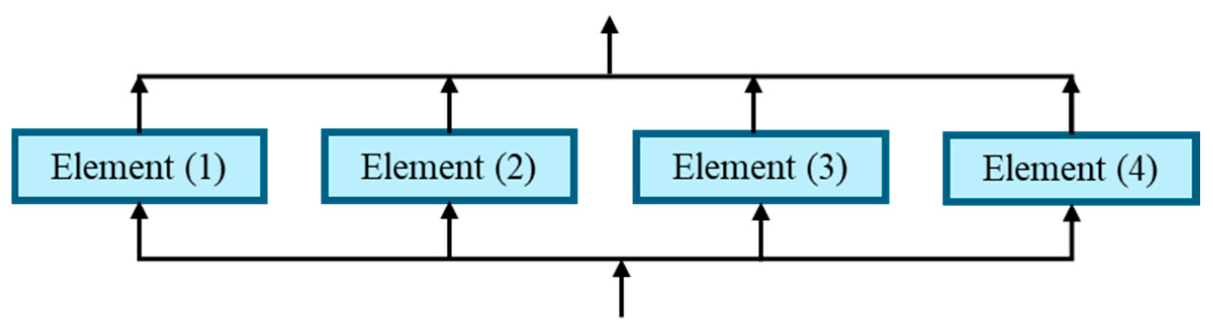
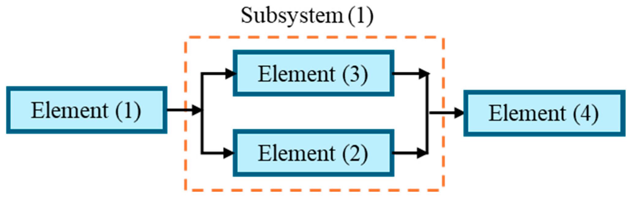
Hence, for very large and complex structures the overall system probability of failure can become dangerously high based on the law of statistical probability. Ref. [35] defined structural system reliability as the probability that the system remains functional and safe even when some of its elements or components fail. The weakest link, or element-based approach, fails to account for the potential redundancy or robustness based on the topology of the structural system. Ref. [36] states that the primary aim of structural reliability analysis and optimisation is to estimate the probability of a failure event to inform risk. Typical structural reliability system topologies are outlined below for series, parallel, and mixed systems as shown in Figure 20, Figure 21 and Figure 22, respectively, based on [4,37].
- Series System
Figure 20.
Systems with elements in series, (Adapted from [4]).

- Parallel System
Figure 21.
Systems with elements in parallel, (Adapted from [4]).
- Mixed System
Figure 22.
Systems with parallel and series elements, (Adapted from [4]).
A comprehensive explanation of classical reliability system theory for parallel, series, and mixed systems can be found in [4,13,16]. These concepts have been further extended and are outlined below in the context of bridge structures, which serve as demonstration analyses in this paper.
2.3. Demonstrated Systems
2.3.1. Bridge Elements in a Series System
To reduce complexity and to better explain the research, only single span structures will be considered in this paper. Figure 23 shows a configuration of typical bridge elements arranged in a simple series system, consisting of a deck slab, abutments, and spread foundation pads. In this arrangement, the elements act sequentially, with each one following the other in a linear order modelled by a simple Bayesian Network.
Figure 23.
Series System in the form of a simple bridge structure.
The probability of structural system failure is given by the sum of the individual element failure probabilities.
where
- P(S)Bridge is Probability of Bridge System Failure
- P(E)DS is Probability of Deck Slab Failure
- P(E)Abut is Probability of Abutment Failure
- P(E)Found is Probability of Foundation Failure
However, when dealing with very small numbers for element failure probabilities, it is more convenient to use the complement of the element probability, that is, the element reliability (sometimes referred to as the probability of survival or success). For a bridge element, this can be expressed as follows.
Hence, the system reliability can be calculated using the following general reliability equation [4].
where
- Rs is system reliability or probability of survival
- Ri is element reliability or probability of survival
- Pi is element reliability or probability of failure
When applied to the bridge elements in Figure 7, the system reliabilities can be calculated as follows.
By inspection, if the abutments and foundations are subject to the same load effects, (flexure, shear, and axial tension or compression) and have the same structural resistances, then Rsa = Rsb if the abutment and foundation elements had the same resistances but were subjected to different load effects, either due to variations in deck restraint allowing articulation or because of ground settlement. It is common practice to use both free and fixed supports (restraints) to accommodate thermal expansion, traction, braking, and creep effects, thereby preventing the buildup of large internal forces that could generate damaging stress paths and eventually structural damage (failure). The system reliability would then be the minimum of Rsa or Rsb, i.e., the lowest possible value of system reliability.
Consider the bridge example in Figure 23, where the reliability indices of all structural elements are optimised to the target reliability level specified for Reliability Class (2) or RC2 in accordance with BS EN 1990 [10,11]. For an Element Reliability Index of 3.8, the corresponding element probability of failure is Pi = 7.2 × 10⁻⁵.
The results shown in Table 9 indicate that the bridge structure is damaged or has failed, because the system reliability index is 3.5, which is lower than the element reliability index of 3.8.
Table 9.
Estimation of System Reliability Index for the bridge example.
By setting a system target reliability of 3.8 for Figure 23, it can be shown that each of the three bridge components would require an element reliability index of 4.1.
2.3.2. Bridge Elements in Parallel System
Figure 24 shows a simple bridge deck supported by four steel beams, with each beam resting on bearings that allow deck articulation. This arrangement of interconnected elements, which share the load, is typical of a parallel system, such that if one beam or bearing fails, it may not lead to the failure of the entire structural system. In the event of beam failure, the load is redistributed to adjacent redundant beams, creating a parallel reliability subsystem problem. This property is referred to as system redundancy. Redundancy plays a key role in the parallel subsystem problem and can be defined as the ability of the system or subsystem to safely redistribute loads following the overloading of one or more structural elements. However, assessing redundancy in a structural reliability system is a complex task. To simplify the problem, two types of redundancy are considered and adapted to system structural reliability based on common approaches used in electrical engineering based on [38,39]) as follows:
Figure 24.
Mixed System in the form of a simple bridge structure.
- Active redundancy refers to the ability of a partially loaded structural element to safely accommodate additional load transferred from a failed or overloaded element in the same structural system. Examples of this include load sharing systems, such as closely spaced main beams supporting a bridge deck where not all beams are loaded to full capacity. Hence, some beams retain reserve strength to accommodate load transfer, typically through a stiffness mechanism whereby the stiffness of adjacent beams attracts and redistributes load from an overloaded, deforming beam.
- Passive, or standby, redundancy occurs when a completely unloaded element becomes active and attracts load due to the overloading or failure of another structural element, thereby helping to stabilise the whole structural system. An example of this is fail safe bracing mechanisms commonly used to accommodate earthquake loading.
Based on modelling, the authors found that increasing redundancy generally increases the system or subsystem reliability. However, careful judgement is required to establish whether structural members arranged in parallel will function as passively or actively redundant elements. Several structural reliability methodologies exist to assess the behaviour of structural elements in parallel, of which the classical system approach is outlined below, which is based on the laws of probability [4,13].
where Pi is probability of ith of n structural elements such that Ri = (1 − Pi).
2.3.3. Bridge Elements in a Mixed System
A mixed structural system is a combination of both series and parallel elements working together as an integrated whole structure. Most bridge structures can be classified as mixed systems, with load sharing elements present in nearly all cases. To reduce complexity in reliability assessment, it is often advantageous to decompose the entire structural system down into discrete subsystems for targeted evaluation and analysis. Ref. [40] suggests a systematic approach for addressing both system- and subsystem-level reliability problems. Subsystems in bridge structures commonly comprise the following arrangements.
- Series Subsystem (members in series only).
- Parallel Subsystem (passive redundant members).
- Parallel Subsystem (active redundant members).
- Parallel Subsystem (active and passive redundancy).
Figure 24, Figure 25 and Figure 26 show a four-beams bridge with a corresponding simplified full schematic or Bayesian Network of interrelated individual structural elements, based on the load path from concrete deck slab to concrete piles. The notation was developed by the authors to identify elements in series, such as an abutment depicted as R5.0 (where R denotes reliability, 5 the element number, and 0 indicates a series element).
Figure 25.
Structural System Reliability (Simple Bridge Full Schematic).
Figure 26.
Structural System Reliability Subsystems Schematic.
Elements in parallel follow the same notation, except the last number is 1 or higher, indicating the presence of multiple similar elements in parallel. Based on the bridge structure in Figure 24, two possible system reliability values can be evaluated using the load-path approach, considering the different failure modes such as flexure, shear, axial tension or compression, and combined load effects. Because the calculation can become complex due to the interaction of multiple series and parallel subsystems, it is often useful to divide the whole structure into substructures or load sets, as illustrated in Figure 26. It should be noted that for all structural systems, the aim is to find an optimal target resistance for each element within the whole structure based on the load and action effects acting on that element using a system RBO methodology.
2.4. System Correlation
Correlation is an important property for System RBDO, as it describes the statistical measure of the strength of the relationship between two or more elements in a system. In terms of reliability analysis, it is assumed element and system metrics are linear in nature [4]. Figure 27 shows the relationship between system correlation and the reliability index. A structural system with elements which are strongly correlated is considered interdependent or connected; hence, failure of one element in a strongly correlated system will generally lead to the failure of the entire system (weakest link theory). Conversely, when elements in a system are weakly correlated, they are considered independent or standalone. In this case, the failure of a single element may have a lesser impact on overall system failure.
Figure 27.
Effect of Correlation on System Reliability Index (Probability of Failure), where ρ is system correlation coefficient.
The safety margin bounds method is employed to develop a graphical solution, as illustrated in Figure 28. The system and element correlations can be generated from a correlation matrix considering the following three element matrix describing pairwise or bivariate correlation.
Figure 28.
Graphical Solution of Bounded Safety Margins (Adapted from [37]).
The authors have adopted a method proposed by [37]. Consider a structural system where n is number of elements arranged in series, wherein each element has a safety margin. By accounting for the failure of one element or all elements, the system failure probability can be expressed accordingly.
where
- P(S) is system failure probability
- Φ is normal or gaussian distribution function
- βs is system reliability index
- β is element reliability index
- ρ is system correlation coefficient
Safety Margins
M1 = β1−a1T U
M2 = β2−a2T U
M3 = β3−a3T U
= a1T a2 = = cos ϴ12
= a2T a3 = = cos ϴ23
= a1T a3 = cos ϴ13
- where ϴ12 is the angle between vectors a1 and a2, forming a linear safety margin. Based on [37], the one-dimensional integral formed by the bounded safety margins can be solved based on graphical representation, as shown in Figure 28.
Using the advanced trigonometry principles, the authors derived the following equation for calculating the angle between two vectors. When rearranged in terms of safety indices, this formulation was found suitable for estimating the local element bivariate (pairwise) correlation coefficient.
The same approach can be applied to all other values of ϴ to construct the correlation matrix. Once complete, this matrix can be used to estimate an average system correlation coefficient as outlined in [37], based on first term of the Taylor expansion.
For example, consider the following tables of results in Table 10 and Table 11, from which the average system correlation coefficient can be calculated.
Table 10.
Element Reliability Results for Simple Bridge in Figure 23.
Table 11.
Estimate of correlation coefficients between elements.
Based on the above results, the local correlation matrix below can be developed, together with an estimate of the average system correlation coefficient.
2.5. Structural System Robustness and Redundancy
2.5.1. Robustness and Redundancy in Limit State Design
A whole structural system consists of a combination of individually designed structural elements interacting in series or parallel, either alone or in subsystems. The local failure of an individual element may have a significant effect on the whole or global structural system safety. Ref. [41] suggested that all elements of a system are subject to two types of failure: soft failure, resulting from deterioration, and hard failure, caused by external shocks. These failures may occur through one or more scenarios, acting singly or in combination.
- Structural deterioration or degradation such as corrosion or water penetration.
- Member capacity reduction due to secondary effects such as bracing failure.
- Fatigue due to cyclic loading and over stressing.
- Overloading beyond the element’s design envelope (abnormal loads).
- Accidental loading such as vehicle impact loading.
A local failure of one element can trigger a cascade failure event, wherein the load carried by the failed element or elements is redistributed to adjacent structural elements, potentially causing them to become overstressed and fail. This process can lead to progressive failure of the entire structure, culminating in global system collapse. This phenomenon is commonly referred to as disproportionate collapse, where a significant portion or the entire structure fails due to the failure of one or more minor elements. To prevent disproportionate collapse scenarios in practice, whole structural systems are often designed with minimum levels of redundancy and robustness, although these properties are difficult to quantify conventionally. Structural design codes often specify minimum levels for tying elements together to mitigate the effects of disproportionate collapse, a concept often referred to as structural string theory. This approach uses multiple strong connections to effectively integrate different elements together, forming a pseudo monolithic structure that enhances load redistribution. Another common approach is key element design, in which critical structural elements in a structure are deliberately over-designed to prevent disproportionate collapse. Refs. [42,43] proposed using a structural reliability-based approach to derive redundancy and robustness metrics for a whole structural system. This approach appears to have been originally developed from ISO 19902 [44] and further extended by this recent research. The approach is based on Hooke’s Law [45], treating the whole structural system as if it behaves like a single structural element. When an external load effect (E) is applied, it is resisted through structural deformation governed by the system’s resistance (R) in accordance with the principle of virtual work.
Now consider the deformation underload of a ductile structure using the Hooke’s Law [44] analogy, as shown in Figure 29.
Figure 29.
Structural element or whole system stress and strain response. (Adapted from [45,46]).
In the context of system structural reliability, Figure 30 presents a simplified version of Figure 29. This simplification highlights the key outcomes that should be considered when assessing the redundancy and robustness of a structural system, which can be outlined as follows:
Figure 30.
Simplified whole system response in terms of stress and strain. (Adapted from [43,46]).
- The Initial Failure State (IFS) is defined as a condition in which the structural system is loaded just beyond its elastic limit, potentially causing localised failure of one or more structural elements. Such failures are accommodated by the system’s inherent redundancy [46].
- The Ultimate Limit State (ULS) represents the ultimate loading of a structural system or single element can sustain while still meeting the prescribed deformation, stress, strain, or other performance criteria. Loading beyond the ULS marks the onset of loss of functionality, permanent damage, and irreversible deformation [46].
- The Ultimate Failure State (UFS) is defined as the point at which a structural system or element experiences complete failure, losing all functionality or efficacy due to unacceptable damage. This occurs when the structure or element is subjected to overloading that generates excessive deformation, stresses, or strains ultimately leading to failure [46].
- The Damage Limit State (DLS) or Damage Limitation State in BS EN 1998 [43], is defined as the ability of a structure or element to maintain an adequate level of reliability against unacceptable damage. This is achieved by satisfying prescribed limits of deformation, stress, and strain, thereby ensuring a minimum level of efficacy or functionality (BS EN 1998 [46]).
The probability of whole system failure (PSF) resulting from various damage scenarios (D) that may arise from multiple hazards (H) can be expressed using a generalized system failure probability equation, as proposed by [43]. For clarity, societal and economic costs have been omitted in this simplified formulation.
where
In a similar manner to structural element design, whole system structural failure should be limited to an acceptable target level, PSF < P(Limit), which can be represented in terms of reliability index β, derived from the normal standard probability distribution. According to the standard BS EN 1990 [10,11], system reliability index limits vary across different classes of structures as below. These limits can be interpolated to determine the minimum acceptable reliability indices based on element design for a 50-year return period.
- Minor or low risk structures, RC1 = 3.3
- Intermediate or medium risk structures, RC2 = 3.8
- Complex or high-risk structures, RC3 = 4.3
The design reliability index for the Damage Limit State (EDLS) is more difficult to determine. However, the approach used in BS EN 1998 [47] with reference to condition factors can be used indirectly with the following sensitivity analysis methodology. It can be shown that there is a direct correlation between applying a condition factor to the system or element resistance and the reliability index using log normal or normal probability distributions with the standard refence models for modal failure. The higher the EDLS, the more onerous the value is in terms of system reliability index. Ref. [48] proposed an EDLS factor of 0.7, although [49] suggested 0.5. Further analysis by the authors showed that an EDLS value of 0.6 provides a reasonable estimate to achieve a minimum 95% system survival probability, avoiding the need to increase element design resistance beyond the limits specified in BS EN 1990 [10,11] to satisfy Damage Limit State requirements (see Table 12). Consequently, the probability of system failure design criteria can now be developed using various limit state load factors. The level of redundancy and robustness of a particular structural design can then be assessed in terms of reliability index using the approach proposed by [42] and modified by the authors for compliance with BS EN 1990 [10,11] as follows.
where Cs is the system factor, Rs is the system reliability index, and ɣsd,i and Pi are individual load factors and probabilities of failure for the whole system. Therefore, considering the three Eurocode classes RC1, RC2, and RC3, it is now possible to develop the various system limit state reliability indices, as presented in Table 12.
Table 12.
Limit State Reliability Indices, (Structure Survival Probability > 95% or β > 1.7).
- Cs < 1.0 indicates a low level of whole system redundancy and robustness (under design).
- Cs > 1.0 indicates a high level of whole system redundancy and robustness (over design).
- Cs = 1.0 indicates optimum whole system redundancy and robustness (optimal design).
With the Limit State Reliability Indices now estimated, the system difference limits for robustness and redundancy can be derived by subtracting the Limit State from the corresponding target reliability indices. This is presented in Table 13.
Table 13.
System Difference Limits (Eurocode Target Reliability Indices).
The system reliability index βULS is obtained by multiplying the mean structural element resistances (µR) by a resistance coefficient (CR) of 1.2 and then recalculating the element and system reliability indices. Similarly, the resistance coefficient for each of the limit states is applied to determine βUFS and βDLS.
- βUFS = System Reliability Index, all structural elements multiply resistance by CR = 1.3.
- βULS = System Reliability Index, all structural elements multiply resistance by CR = 1.2.
- βDLS = System Reliability Index, all structural elements multiply resistance by CR = 0.6.
2.5.2. Robustness and Redundancy Metrics
Ref. [50] highlighted the need for risk assessment related to disproportionate collapse for modern structures, but concluded that there is still no consensus on the definition or standardised estimation of robustness in whole structural systems. Building on the work of [49,51], the authors developed robustness and redundancy metrics that yield a percentage measure, providing an easily interpretable alternative to existing methods, which often range from zero to infinity or are complex to calculate. Ref. [43] defined structural robustness as the capability of a structure in a damaged state to continue in normal service independent of all of the hazards that caused the initial damage. Therefore, there is a direct relationship between the structure in its original service condition βULS and in an existing damaged state βDLS, allowing the reserve capacity of the structure to be measured. Based on this, a simple indicative measure of robustness can be evaluated as follows:
Based on the target limits presented in Table 13, the target robustness should be >50% in an undamaged state. This approach raises a problem: What if βDLS falls below the safe target limit, such that the structure effectively becomes unsafe to use in normal service? The above equation could still provide a comfortable level of robustness in a failure state. Introducing safety target limits from Table 13 and considering the logarithmic scale of reliability indices, the robustness of a safe structure could be evaluated as follows.
Redundancy was defined by [43] as the capability of the intact structure to maintain normal service loads following the failure of one or more structural elements. Similarly, there is a direct relationship between the original structure in the normal service βULS and the existing structure in a damaged state βDLS, where the damage limit state is calculated following failure of one or more elements. Ref. [49] proposed that a simple indicative measure of redundancy could be evaluated as follows.
This approach again has the issue of omitting any safety limit. Hence, an unsafe structure could be considered to have structural redundancy. Thus, a revised approach to both yield a percentage and include safety limits was developed; the revised approach governs the following equations.
Using the target values presented in Table 12, sensitivity analysis was employed to determine the optimal safe values of robustness and redundancy. The results presented in Table 14, Table 15 and Table 16 were obtained by adjusting βULS to estimate Ired and Irob.
Table 14.
Robustness and Redundancy Indices (βULS = 3.3).
Table 15.
Robustness and Redundancy Indices (βULS = 3.8).
Table 16.
Robustness and Redundancy Indices (βULS = 4.3).
The simple sensitivity analysis presented in Table 14, Table 15 and Table 16 indicates that robustness and redundancy are closely aligned with the indices being approximately constant for each class of structure. It should be noted that the robustness and redundancy indices are indicative. More accurate measures of robustness and redundancy can be obtained through a complex sensitivity analysis that evaluates the impact of damage to one or more elements in the structure simultaneously [52]. However, this approach is beyond the scope of this paper.
2.6. Computational Study
Using the framework of system difference limits proposed by [42], it is possible to assess both the correlation redundancy and robustness of whole structural systems. Consider a series system in the form of the bridge structure example as shown in Figure 23 if all elements had a reliability index of 3.8, such that the system reliability index was 3.5.
Assume this is a RC2 structure with a target reliability index of 3.8, only flexure is considered in this example using standardised reference model parameters for element and system design. Based on this example, the simple bridge structure fails to meet minimum robustness and redundancy requirements and is redesigned.
Mean Slab Element Load Effect Mkyy = 150 kNm,
Mean Element Load Effect Mkyy = 45 kNm,
Mean Foundation Element Load Effect Mkyy = 75 kNm,
Load Effect Covariance vE = 0.1, (Lognormal Distribution)
Resistance Covariance vR = 0.15, (Lognormal Distribution)
Mean Characteristic Load Effect Coefficient = 1.0
Mean ULS Resistance Coefficient = 1.2
The results of the system difference limits analysis are outlined in Table 17 and Table 18, which show that although the elements comply with the modal failure reliability index, the system difference limits analysis fails.
Table 17.
System Difference Limits (Bridge structure in Figure 7).
Table 18.
System Difference Limits (Limit States—Bridge structure in Figure 23).
The optimum redundancy and robustness can be estimated by identifying the area experiencing the greatest failure and recalculating the minimum system element reliability required, with a minimum βDLS ≥ 2.0. This can be determined iteratively by working backwards to find the minimum element reliability index as defined as optimisation, as shown in Table 19, Table 20 and Table 21.
Table 19.
Minimum Damage Limit State Index using Optimisation.
Table 20.
System Difference Limits using Optimisation.
Table 21.
Updated System Limit Metrics using Optimisation.
Based on calculation, the minimum optimum element βULS of 3.8, (FOS = 1.6), subject to system optimisation, would need to be increased to 6.3 (FOS ~2.6), to satisfy the robustness and redundancy requirements of the structural system damage limit state. This represents an increase of approximately 50% in design resistance. Due to a high system correlation, element failure (weakest link approach) would be dominant; hence, the element optimisation approach may be valid at reduced system safety metrics for one mode of failure.
2.7. Optimisation Approach
The whole system optimisation problem is nested, requiring a staged approach to consider the modal, combined, and system failure probabilities to be found using the methodology outlined in Figure 31, Figure 32, Figure 33 and Figure 34. This novel approach was applied to a simple concrete footbridge pilot study (see Figure 35 and Figure 36) as outlined below.
Figure 31.
Multimethod RBDO Modal Failure (Source Author).
Figure 32.
Weighted Combined Failure RBDO (Source Author).
Figure 33.
System Difference Limit Reliability Optimisation Method.
Figure 34.
Outline Flowchart of Optimisation Methodology.
Figure 35.
Individual Elements of the Concrete Footbridge, (Source Author).
Figure 36.
Concrete Footbridge Load Path Schematic and Structural System Reliability.
Stage (1)—The footbridge was designed using proprietary computer software and hand calculations to comply with the deterministic requirements of the Eurocodes. This provides a baseline model for comparison.
Stage (2)—The footbridge elements were checked using the reliability index multi-method to assess each potential mode of failure, which delivered an envelope of reliability indices. This approach yields the optimum modal element design resistance for the target reliability index and yields the percentage of modal element resistance over or under design, see Figure 31.
Stage (3) The check was extended to assess the combined modal element resistance based on utilising the revised target reliability index for each mode of failure. A weighted gradient optimisation was employed to yield minimum modal resistances to satisfy the combined element target reliability index.
The weighting mechanism was based on load effect magnitude to generate the minimum safe baseline reliability indices for all structural elements in the system for both modal and combined failure scenarios. See Figure 32.
Stage (4) The system optimisation approach required the development of a load-path reliability model or Bayesian Network for the structure to calculate the system reliability indices. The system difference limits were calculated to determine whether these were satisfied by the initial structural design. If the system limits were not met, weighting factors were applied to ensure that only the weakest and lowest element resistances were increased/strengthened, thereby minimising both cost and material usage. For example, it is generally more expensive and requires more steel reinforcement to strengthen a heavily reinforced main beam than to upgrade a small steel bearing. The iterative loop approach updated the element reliability indices and resistance parameters, which fed back into the Bayesian Network as a closed loop until the system limits were satisfied. Finally, a secondary check was undertaken to ensure the minimum modal and combined effect reliability indices were maintained. See Figure 33.
The optimisation problem involves increasing the reliability index of the weakest elements—those with the lowest element resistance values—until the system difference limits are satisfied. The key to success is the weighting mechanism, which comprises three components:
- ○
- The element weighting, calculated as the inverted coefficient of the element resistance divided by the sum of all element resistances,
- ○
- The subsystem weighting, calculated as the inverted coefficient of the sum of sub-system element resistances divided by the sum of all element resistances, and
- ○
- The failure probability of the element, obtained from the previous iteration of the reliability index.
Stage (5)—The footbridge elements were reviewed for potential reductions or increases in element resistance to meet the optimal target reliability index element resistance requirement. This approach is constrained by the need to comply with Eurocodes to meet the Bolam Test’s [53] duty of care legal authority.
Stage (6)—Estimate savings in terms of cost and material due to over/under design were developed based on changes to the design using a pragmatic approach. Based on testing, some savings will be theoretical based on deterministic code requirements relating to secondary design constraints and detailing rules. The whole RBDO process is outlined in Figure 34 below.
3. Results and Discussion
The proposed approach was extended to a simple footbridge designed to the Eurocodes using the proprietary software TEDDS version 1.0.22 and SCALE version 4.1 (see Figure 35 and Figure 36). The reliability optimisation was modelled using Excel Spreadsheets, which could theoretically link to a Revit version 2024.02 BIM model and be validated using CodeCal version 03 reliability software. By applying the optimisation approach, the robustness and redundancy metrics of the structure could be assessed. Assuming standardised reference model parameters, system difference limit optimisation was applied with an initial target reliability index βULS = 3.8 to generate results. Initial values of shear Vyy and Vzz were previously optimised to the element modal target reliability index, while Flexure Myy and Mzz and axial effects Nxx were previously optimised for combined modal failure effects of the elements.
The results presented in Figure 37a,b are for the initial unoptimised system based on a deterministic Eurocode design. They show that most system-level modal failure scenarios are satisfied, except for shear Vzz and Vyy, both of which fail to meet the damage limit state requirement. Based on the system correlation, the lowest element reliability index, (βULS = 3.8), would govern the failure mode of the structure in line with ‘weakest link’ theory. The relatively high system reliability indices also suggest that several elements are over designed and could, in principle, be reduced without compromising overall performance.
Figure 37.
(a) System Reliability analysis of footbridge using Eurocode design method. Note (1). Flexure Myy and Mzz satisfy the system difference limits but the structure is deemed overdesigned based on the high values of the reliability index limit states. Note (2). Shear Vyy satisfies the system difference limits for ULS and UFS limit states and could be deemed overdesigned. However, the DLS or Damage limit state fails, making this mode of failure more prone to premature failure. Note (3). Based on the results of Myy, Mzz, and Vyy, the initial design forming the structural system is not balanced and the ratio of system safety to economy is suboptimal. (b) System Reliability analysis of footbridge using Eurocode design method. Note (4). Shear Vzz satisfies the system difference limits for ULS and UFS limit states and could be deemed overdesigned. However, the DLS limit state fails, making this mode of failure more prone to premature failure. Note (5). Axial Nxx satisfies the system difference limits but is deemed overdesigned based on the high values of the reliability index limit states. Note (6). The summary of system parameters indicates potential overdesign of some elements. The large difference between the minimum system and element ULS reliability indicates an unbalanced system. The system correlation also indicates a suboptimal system, as this indicates a wide variance of element reliability indices, (for all elements the same correlation tends to 1.0).
The results presented in Figure 38a,b are for the optimised structure, expressed in terms of system difference limits using the proposed System Structural RBDO method. They show a general reduction in reliability indices while still satisfying all modal failure scenarios. System values are governed by the minimum indices. This optimisation approach also satisfies the damage limit state requirement, albeit with a minor reduction in the robustness and redundancy indices. Consistent with the system correlation, the lowest element reliability index, (βULS = 4.2), dominates the structural failure mode.
Figure 38.
(a) System Reliability analysis of the footbridge using System RBDO. Note (1). Flexure Myy, Mzz, and shear Vyy satisfy all limit states and safety indices. The ULS and UFS limit states have reduced, indicating reduced resistance and material requirements providing an improved or optimal balance between safety and economy. It should be noted that redundancy and robustness indices tend to reduce but are still satisfactory. (b) System Reliability analysis of the footbridge using System RBDO. Note (2). Both shear Vzz and Axial Nxx failure modes satisfy all limit states and safety indices. The ULS and UFS limit states have reduced, indicating reduced resistance and material requirements providing an improved or optimal balance between safety and economy. It should be noted that redundancy and robustness indices tend to reduce but are still satisfactory. Note (3). Overall, the system parameters have reduced slightly in terms of correlation, robustness, and redundancy indices; however, these still satisfy minimal safety limits. The minimal system ULS reliability index has reduced, while the minimum element ULS reliability index has increased to almost equalise presenting a more balanced or optimal structural system in terms as these safety metrics of safety and economy. Note (4). Due to the requirement to satisfy the combined effects constraint on element reliability index, it was not possible to satisfy the exact difference limit state parameters.
The optimisation indicates approximately a fivefold reduction in structural failure probability. A notable outcome is the convergence of the system and element reliability indices βULS. However, due to the constraints of the combined element reliability indices on the system difference limits, perfect optimisation could not be achieved, resulting in a slightly higher βDLS than the optimum value of 2.0.
Table 22 shows the change element resistances from the initial Eurocode design or assessment of the structure to the optimised design using the system difference limits using the proposed System Structural RBDO method. Generally, theoretical element resistances reduce, except for the bearings, which require strengthening based on the weighted optimisation approach. This is because the smallest elements were the ones upgraded the most. Although some of the uplift values may appear excessive, the actual increases in element resistance are often relatively modest for bridge design. For example, a fixed bearing in flexure Myy with an uplift of 169% required an increase in strength from 20 kNm to 54 kNm to satisfy the system damage limit state for robustness and redundancy. Conversely, some of the larger reductions in element resistance may be impracticable due to secondary constraints.
Table 22.
System Optimisation (Theoretical Element Resistance Change).
Table 23 reveals the element reliability indices based on the system difference limit optimisation. Due to the weighting mechanism, the elements with the lowest initial resistance and reliability index have been upgraded the most, thereby minimising the cost and material usage resource. In general, the most expensive elements to strengthen are upgraded the least, leading to a lowest cost sustainable solution. Using a confidence interval approach, it can be seen that a ULS element reliability index of 6.2 or more will generally satisfy the requirements of the system difference limits approach for this example.
Table 23.
System Optimisation Element Reliability Indices. (Statistical measures based on [32]).
Table 24 compares three different scenarios for the concrete footbridge example. The initial deterministic Eurocodes design, without optimisation, satisfied the system difference limits approach but still offered scope for improvement to reduce both cost and material use.
Table 24.
Average System Modal Reliability Indices. (Note: * represents system failure.)
The element-level optimisation in compliance with the Eurocodes failed to satisfy the damage limit state requirement and could therefore be considered vulnerable to disproportionate collapse due to insufficient redundancy and robustness.
The system optimisation using difference limits showed a general marginal reduction in reliability indices, enabling cost and material savings by allowing reductions in element resistances. This translates into lower steel reinforcement requirements or reduced section thicknesses.
In contrast, during the element Eurocode optimisation for several elements, element resistance reduction was constrained by combined element load effects. A theoretical average reduction of 15% in element resistances could, in practice, translate into substantial cost and material savings in real terms provided that all secondary design constraints are satisfied.
In this case study, the main concrete beams and bearings would require upgrading, in theory. On inspection, the material and carbon costs of any such upgrade would be nominal for the following reasons. The main beam requires additional main reinforcement, which will be balanced by savings in shear and secondary reinforcement. The bearing upgrade would effectively still utilize the same size bearings, as these tend to be standardised and set to the desired loading requirements. Hence, based on the results, the following elements were reviewed and rechecked for compliance with the Eurocodes, with the following results.
- Deck slab—steel reinforcement (B12 bars to B8 bars).
- Bankseat—concrete depth reduced (1000 mm to 600 mm).
- Piles—steel reinforcement (B25 bars to B16 bars, links reduced from B12 to B8).
The resistances relating to the above changes for the reliability analysis were altered accordingly for a selective optimisation as a pragmatic approach, see Table 25 and Table 26. Element resistance is optimised subject to structural code constraints relating to minimum concrete cover and minimum reinforcement requirements to ensure ductile failure, deflection, cracking etc.
Table 25.
Estimated material cost and Carbon Savings, (Pragmatic Approach).
Table 26.
Equivalent Carbon Estimates (Adapted from [54]).
4. Conclusions
The results indicate that the proposed System Structural Reliability Based Optimisation (RBDO) is a safer approach than the direct element reliability-based optimisation. The system-based optimisation approach considers both the redundancy and robustness of the whole structure, although it may result in marginally higher element resistances to satisfy the considered design limit states. This is because the system reliability optimisation is constrained to ensure that minimum target reliability indices or acceptable probabilities of failure are achieved for all elements. The primary advantage of system RBDO is that a better balance between safety and economy is achieved. The system RBDO approach provides a holistic and balanced method by considering multiple failure modes, thus enhancing overall structural safety.
The demonstrated system of reliability analysis for the footbridge using the proposed system RBDO approach reveals that it can validate and reduce the over-design of elements. This enables significant benefits in reducing both cost and material use at the design stage. Ref. [55] showed that material costs account for 60% of the total costs of new highway structures. Ref. [56] detailed £1.2 Billion spent on new highways structures in 2025. Hence, a 15% reduction in material cost could potentially lead to an annual savings of over £108 million on the UK strategic road network.
The proposed novel approach breaks down the traditional barriers to RBDO in mainstream practice, yielding key benefits outlined as follows.
- Enhances structural safety, with results that are easy to interpret in terms of over design percentages, reliability indices, (safety indices), and system robustness and redundancy indices.
- Ease of use, with standardised equations that eliminate the need to develop and solve limit state equations using calculus.
- Highlights over-designed elements, allowing for easy review and value engineering.
- Enable rapid and easy calculations that can be integrated/encoded into conventional Building Information Modelling (BIM) software. Prefabricated elements or structures can be imported into the models with predetermined element resistance values. Additionally, the BIM model can highlight under-designed and potentially dangerous elements with an intuitive dashboard, either during the design stage or in service if load effects change significantly.
- Both system- and element-based RBO design models can be used for future structural assessment during the in service or asset management stage, offering potentially significant savings in terms of time and resources for maintenance.
The proposed RBDO approach is considered an effective and efficient method for both designing and checking highway (bridge) structures, providing additional insights into element correlation, system robustness, and redundancy. The methodology, which uses target reliability indices to determine optimal structural element and system resistances, can be semi-automated using standard reference models and integrated into BIM and is now regarded as a proven concept. The primary challenge in structural design is obtaining the initial load and action effects on structure elements, which must be determined through a combination of structural analysis and reference to deterministic codes of practice. This also applies to deriving element resistances using deterministic design approaches or traditional structural codes of practice.
Element-level RBDO can be validated using existing structural software based on deterministic design methods. By optimising the parameters in software such as SCALE or TEDDS, it is possible to compare the element design resistances between the two approaches. Validating system-level RBDO is more challenging, as no alternative method currently exists to directly measure structural system correlation, robustness, and redundancy metrics. The system reliability index can be benchmarked against CS 451 [57,58], which recommend an average notional value of (βULS = 5.6) for new bridge structures. This equates to a system failure probability of 10−8 for bridges complying with modern design codes.
Probabilistic design methods such as RBDO are not yet widely adopted in the construction industry, due to the sophistication of modern structural design codes and the presence of multiple, sometimes conflicting, constraints. However, both element- and system-RBDO offer real benefits to the design process in terms of reducing both client and environmental costs. Additional benefits of system RBDO include the direct derivation of system safety metrics, which is not feasible via element-based traditional structural design. The approach also enables the monitoring and management of safety metrics within a reliability BIM based asset management model in service as the structure deteriorates or suffers damage. This can be achieved through structural health monitoring devices, allowing monitoring of the structural system safety indices of a highway structure in real time. Alternatively, periodic structural inspections could be used to generate structural element condition indicators, which could then be used to update the BIM model using a reliability-based approach.
The limitations of this research paper can be outlined as follows. The scope of testing includes single span bridges to prove the concept. Once the RBDO BIM model is established, it offers multiple opportunities for future research, which include:
- Developing the link between RBDO and BIM model for generative design.
- Improve bespoke element design using multivariate RBDO using approaches such as the Rosenblatt Transformation Method.
- Structural health monitoring SHM and RBO maintenance scheduling.
- Modelling element and whole structure deterioration, possibly using Markov Chains or similar approaches.
- Incorporating the element and system RBDO approaches into a Monte Carlo Simulation to assess any differences in results of the methods and potentially refine the approach.
Author Contributions
Conceptualization, J.D. and B.C.; methodology, J.D., B.C. and V.B.N.; software, J.D.; validation, J.D., B.C. and V.B.N.; formal analysis, J.D.; investigation, J.D., B.C. and V.B.N.; resources, J.D., B.C. and V.B.N.; data curation, J.D.; writing—original draft preparation, J.D.; writing—review and editing, J.D., V.B.N. and B.C.; visualization, J.D.; supervision, B.C., V.B.N.; project administration, J.D., B.C.; funding acquisition, J.D, B.C. and V.B.N. All authors have read and agreed to the published version of the manuscript.
Funding
This research received no external funding.
Data Availability Statement
The original contributions presented in this study are included in the article. Further inquiries can be directed to the corresponding author(s).
Acknowledgments
The authors would like to thank the anonymous reviewers for their constructive comments towards improving the quality of this paper.
Conflicts of Interest
The authors declare no conflicts of interest.
References
- Gholam, B. What do we mean by efficiency? A holistic approach to reducing embodied carbon. Struct. Eng. 2020, 98, 14–17. [Google Scholar] [CrossRef] [Scilit]
- Webster, M.D. Achieving Net Zero Embodied Carbon in Structural Materials by 2050. 2020. Available online: https://www.researchgate.net/publication/340738973_Achieving_Net_Zero_Embodied_Carbon_in_Structural_Materials_by_2050 (accessed on 10 November 2025).
- Hackitt, J. Building a Safer Future: Independent Review of Building Regulations and Fire Safety: Final Report. Department for Housing, Communities and Local Government. 2018; p. 39. Available online: https://assets.publishing.service.gov.uk/media/5afc50c840f0b622e4844ab4/Building_a_Safer_Future_-_web.pdf (accessed on 11 November 2025).
- Schneider, J. Reliability of Structures (SED 5), 3rd Reviewed and Extended Edition; IABSE: Zurich, Switzerland, 2017; pp. 1, 81–87. ISBN 1523112743. Available online: https://jochenk.folk.ntnu.no/SED5_3rd_edition.pdf (accessed on 13 April 2024).
- Ellingwood, B.R. LRFD: Implementing structural reliability in professional practice. Eng. Struct. 2000, 22, 106–115. [Google Scholar] [CrossRef] [Scilit]
- Melchers, R.E.; Beck, A.T. Structural Reliability Analysis and Prediction; John Wiley & Sons: Hoboken, NJ, USA, 2018. [Google Scholar]
- Haldar, A.; Azizsoltani, H.; Gaxiola-Camacho, J.R.; Vazirizade, S.M.; Huh, J. Reliability Evaluation of Dynamic Systems Excited in Time Domain REDSET: Alternative to Random Vibration and Simulation; John Wiley & Sons: Hoboken, NJ, USA, 2023. [Google Scholar]
- Benjamin, J.R.; Cornell, C.A. Probability, Statistics, and Decision for Civil Engineers; Dover Publications, Courier Corporation: New York, NY, USA, 2014. [Google Scholar]
- Nowak, N.A.S.; Collins, K.R. Reliability of Structures; CRC Press: Boca Raton, FL, USA, 2012. [Google Scholar]
- BS EN 1990; Eurocode 0—Basis of Structural Design (+A1:2005) (Incorporating Corrigendum December 2008). British Standards Institution: London, UK, 2002.
- BS EN 1990; Eurocode 0—Basis of Structural and Geotechnical Design. British Standards Institution: London, UK, 2023; ISBN 9780539041491.
- ISO 2394; General Principles on Reliability for Structures. CS Code (Structures of Buildings in General): 91.080.01. International Standards Organization: Geneva, Switzerland, 2015.
- Holický, M. Reliability Analysis for Structural Design; SUN MeDIA: Stellenbosch, South Africa, 2009; pp. 135–140. [Google Scholar] [CrossRef] [Scilit]
- Roscoe, K.; Diermanse, F.; Vrouwenvelder, T. System reliability with correlated components: Accuracy of the Equivalent Planes method. Struct. Saf. 2015, 57, 53–64. [Google Scholar] [CrossRef] [Scilit]
- Bhamare, S.S.; Yadav, O.P.; Rathore, A. Evolution of reliability engineering discipline over the last six decades: A comprehensive review, 2007. Int. J. Reliab. Safety 2007, 1, 377. [Google Scholar] [CrossRef] [Scilit]
- Grandi, R.V.; Wang, L. Structural Reliability Analysis and Optimization: Use of Approximates. NASA/CR-1999-209154, 1999; pp. 232–266. Available online: https://ntrs.nasa.gov/api/citations/19990049421/downloads/19990049421.pdf (accessed on 12 May 2024).
- Beck, A. Optimal Design of Redundant Structural Systems: Fundamentals. Eng. Struct. 2020, 219, 110542. [Google Scholar] [CrossRef] [Scilit]
- Wang, H.; Gong, Z.; Huang, Z.; Zhang, X.; Lv, Z. System Reliability Based Design Optimization with Monte Carlo Simulation, 2012. In Proceedings of the International Conference on Quality, Reliability, Risk, Maintenance, and Safety Engineering, Chengdu, China, 15−18 June 2012; pp. 1143–1147. [Google Scholar]
- Nguyen, T.H.; Song, J.; Paulino, G.H. Single-loop system reliability-based topology optimization considering statistical dependence between limit states. Struct. Multidiscip. Optim. 2011, 44, 593–611. [Google Scholar] [CrossRef] [Scilit]
- Rosenblatt, M. Remarks on a multivariate transformation. Ann. Math. Stat. 1952, 23, 470–472. [Google Scholar] [CrossRef] [Scilit]
- Noh, Y.; Choi, K.; Du, L. Reliability-based design optimization of problems with correlated input variables using a Gaussian Copula. Struct. Multidiscip. Optim. 2009, 38, 1–16. [Google Scholar]
- Wanga, J.; Lib, C.; Xua, C.; Lia, Y.; Kareemd, A. Efficient structural reliability analysis based on adaptive Bayesian support vector regression. Comput. Methods Appl. Mech. Eng. 2021, 387, 114172. [Google Scholar] [CrossRef] [Scilit]
- Denby, P. Computational Engineering; Institution of Structural Engineers: London, UK, 2020; ISBN -10:1906335443. [Google Scholar]
- Gauss, C.F. Theoria Motus Corporum Coelestium; Translation reprinted as Theory of the Motions of the Heavenly Bodies Moving about the Sun in Conic Sections; Perthes: Hamburg, Germany, 1809. [Google Scholar]
- Hasofer, A.M.; Lind, M.C. An Exact and Invariant First Order Reliability Format. J. Eng. Mech. 1974, 100, 111–121. [Google Scholar]
- Rackwitz, R.; Fiessler, B. Structural reliability under combined random load sequences. Comput. Struct. 1979, 9, 484–494. [Google Scholar] [CrossRef] [Scilit]
- Niemann, H.; Diburg, S. Statistics of extreme climatic actions based on the Gumbel probability distributions with an upper limit. Comput. Struct. 2013, 126, 193–198. [Google Scholar] [CrossRef] [Scilit]
- Welch, B.L. The Significance of the Difference Between Two Means When the Population Variances Are Unequal. Biometrika 1938, 29, 350–362. [Google Scholar] [CrossRef] [Scilit]
- Winterstein, R. An Introduction to Structural Reliability. 2011. Available online: https://www.researchgate.net/publication/328150865_An_Introduction_to_Structural_Reliability_FORM_and_LRFD_Design (accessed on 12 June 2024).
- Joint Committee on Structural Safety, JCSS. Probabilistic Model Code for Modern Engineering; PWS Publishers: Zurich, Switzerland, 2001; ISBN 0-534-01460-7. Available online: https://www.jcss-lc.org/jcss-probabilistic-model-code/ (accessed on 13 May 2024).
- Ellingwood, B.R.; Galambos, T.V.; MacGregor, J.G.; Cornell, C.A. Development of a Probability-Based Load Criterion for American National Standard A58; National Bureau of Standards: Washington, DC, USA, 1980. [Google Scholar]
- Lapin, L.L. Probability and Statistics for Modern Engineering; PWS Publishers: Zurich, Switzerland, 1987; ISBN 0-534-01460-7. [Google Scholar]
- BS EN 1992-1-1; Eurocode 2: Design of Concrete Structures—Part 1-1: General Rules and Rules for Buildings. British Standards Institution: London, UK, 2004.
- BS EN 1993-1; Eurocode 3: Design of Steel Structures—Part 1-1: General Rules and Rules for Buildings. British Standards Institution: London, UK, 2005.
- Song, J.; Kang, W.; Lee, Y.; Chun, J. Structural System Reliability: Overview of Theories and Applications to Optimization. ASCE-ASME J. Risk Uncertain. Eng. Syst. Part A Civ. Eng. 2021, 7, 1–19. [Google Scholar] [CrossRef] [Scilit]
- Bai, Z.; Song, S. Structural reliability analysis based on neural networks with physics-informed training samples. Eng. Appl. Artif. Intell. 2023, 126, 107–157. [Google Scholar] [CrossRef] [Scilit]
- Sorenson, J.D. Structural Reliability Theory and Risk Analysis. 2004, pp. 103–166. Available online: https://www.ukm.my/kamal3/rro/note%20Structural%20Reliability%20Theory%20and%20risk%20analysis.pdf (accessed on 11 May 2024).
- Guo, J.; Wang, X.; Liang, J.; Pang, H.; Goncalves, J. Reliability Modeling and Evaluation of MMCs Under Different Redundancy Schemes. IEEE Trans. Power Deliv. 2018, 33, 2087–2096. [Google Scholar] [CrossRef] [Scilit]
- Mok, Y.L.; Goh, C.H.; Segaran, R.C. Redundancy modeling for the X-Sat microsatellite system. In Proceedings of the 2013 Proceedings Annual Reliability and Maintainability Symposium (RAMS), Orlando, FL, USA, 28−31 January 2013; pp. 1–6. [Google Scholar]
- Ginzburg, S.M.; Yudelevich, A.M. Reliability assessment of hydraulic structures. Power Technol. Eng. 2021, 54, 793–801. [Google Scholar] [CrossRef] [Scilit]
- Bian, L.; Wang, G.; Liu, P. Reliability analysis for multi-component systems with interdependent competing failure processes. Appl. Math. Model. 2021, 94, 446–459. [Google Scholar] [CrossRef] [Scilit]
- Ghosn, M.; Moses, F. Redundancy in Highway Bridge Superstructures, NCHRP Rep, 406; Transportation Research Board: Washington, DC, USA, 1998; pp. 14–16. [Google Scholar]
- Anitori, G.; Casas, R.J.; Ghosen, M. Redundancy and Robustness in the Design and Evaluation of Bridges: European and North American Perspectives. J. Bridge Eng. 2013, 18, 1241–1251. [Google Scholar] [CrossRef] [Scilit]
- ISO 19902; Petroleum and Natural Gas Industries—Fixed Steel Offshore Structures (Updated 2020). International Standards Organization: Geneva, Switzerland, 2002.
- Hooke, R. De Potentia Restitutiva, (or of Spring), Explaining the Power of Springing Bodies; John Martyn Printer to the Royal Society: London, UK, 1678. [Google Scholar]
- Gere, J. Mechanics of Materials, 5th ed.; Nelson Thornes: Cheltenham, UK, 2002; p. 15. ISBN 0748766758. [Google Scholar]
- BS EN 1998; Eurocode 8—Design of Structures for Earthquake Resistance—Part 1: General Rules, Seismic Actions and Rules for Buildings. British Standards Institution: London, UK, 2004.
- Kristiawan, S.A.; Hapsari, I.R.; Purwanto, E.; Marwahyudi, M. Evaluation of Damage Limit State for RC Frame Based on FE Modeling. Buildings 2022, 12, 21. [Google Scholar] [CrossRef] [Scilit]
- Frangopol, D.M.; Curley, J.P. Effects of damage and redundancy on structural reliability. J. Struct. Eng. 1987, 113, 1533–1549. [Google Scholar] [CrossRef] [Scilit]
- André, J. Structural robustness: A revisit. Struct. Eng. Mech. 2020, 2, 1–20. [Google Scholar]
- Lind, N. A measure of vulnerability and damage tolerance. Reliab. Eng. Syst. Saf. 1995, 48, 1–6. [Google Scholar] [CrossRef] [Scilit]
- Frangopol, D.M.; Zhu, B.; Sabatino, S.; Kozy, B. Bridge System Reliability and Reliability Based Redundancy Factors; Federal Highway Administration Office of Infrastructure—Bridges and Structures FHWA-HIF-19-093: Washington, DC, USA, 2019; pp. 6–34. [Google Scholar]
- Bolam v Friern Hospital Management Committee [1957] 1 WLR 582. Available online: https://www.oxfordreference.com/display/10.1093/oi/authority.20110803095515879 (accessed on 15 May 2024).
- Circular Ecology Ltd. ICE Database Inventory of Carbon and Energy, 2024. Available online: https://circularecology.com/embodied-carbon-footprint-database.html (accessed on 12 October 2024).
- Rwamamara, R.; Simonsson, P.; Larsson, J. Advantages of industrialized methods used in small bridge construction. In Proceedings of the IGLC-18, Technion, Haifa, Israel, 18 July 2010; pp. 569–579. [Google Scholar]
- National Highways. Keeping Our Major Roads Running All Year Round Annual Report and Accounts, 2025, p. 13. Available online: https://nationalhighways.co.uk/media/okehxfjy/national_highways_ara_24-25.pdf (accessed on 21 December 2025).
- National Highways. CS451 Structural Review and Assessment of Highway Structures, 2020. Available online: https://www.standardsforhighways.co.uk/tses/attachments/81489ab4-7e79-4139-9822-104fa460cd84?inline=true (accessed on 12 December 2024).
- Atkins. Guidance Document for Performance Measurement of Highway Structures Part B3: Reliability Performance Indicator, 2007. Available online: https://adeptnet.org.uk/sites/default/files/media/2022-11/Guidance%20Document%20for%20Performance%20Measurement-%20Part%20B3%20Reliability%20PI.pdf (accessed on 11 June 2024).
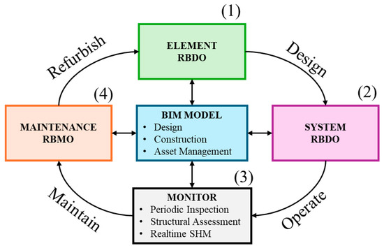
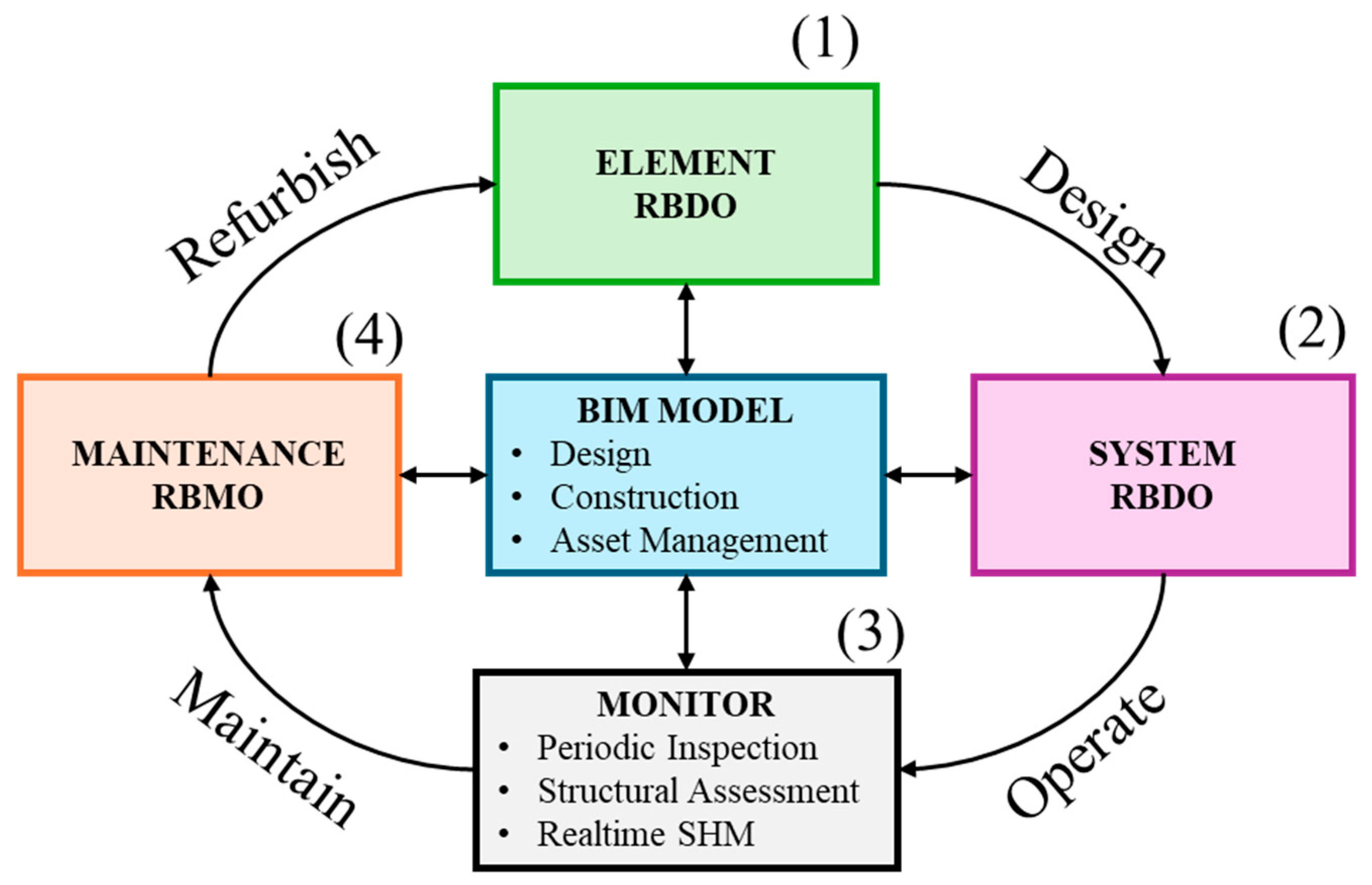
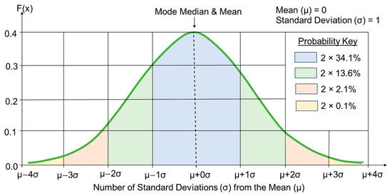
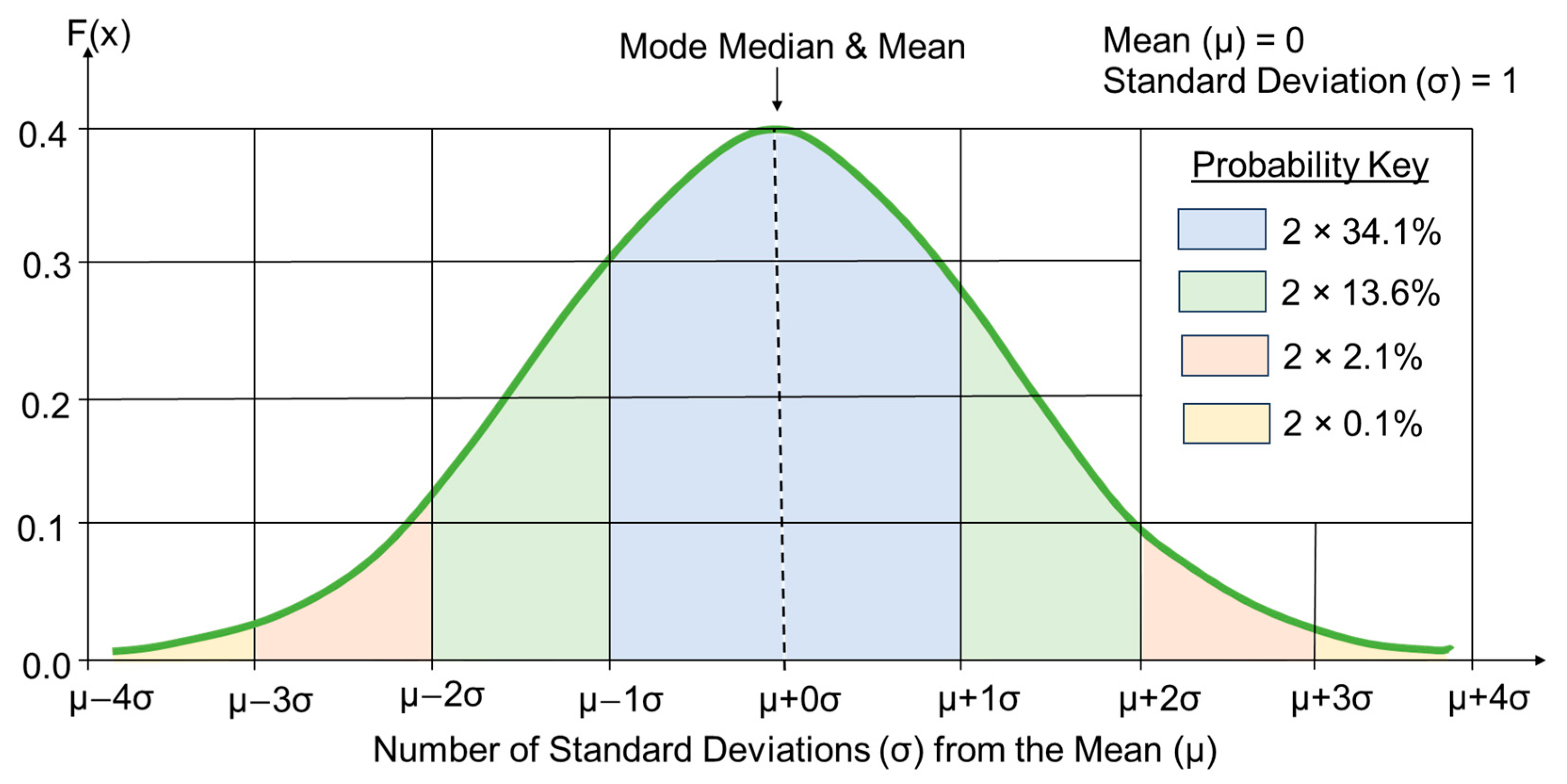
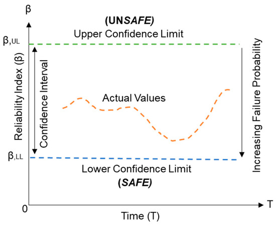
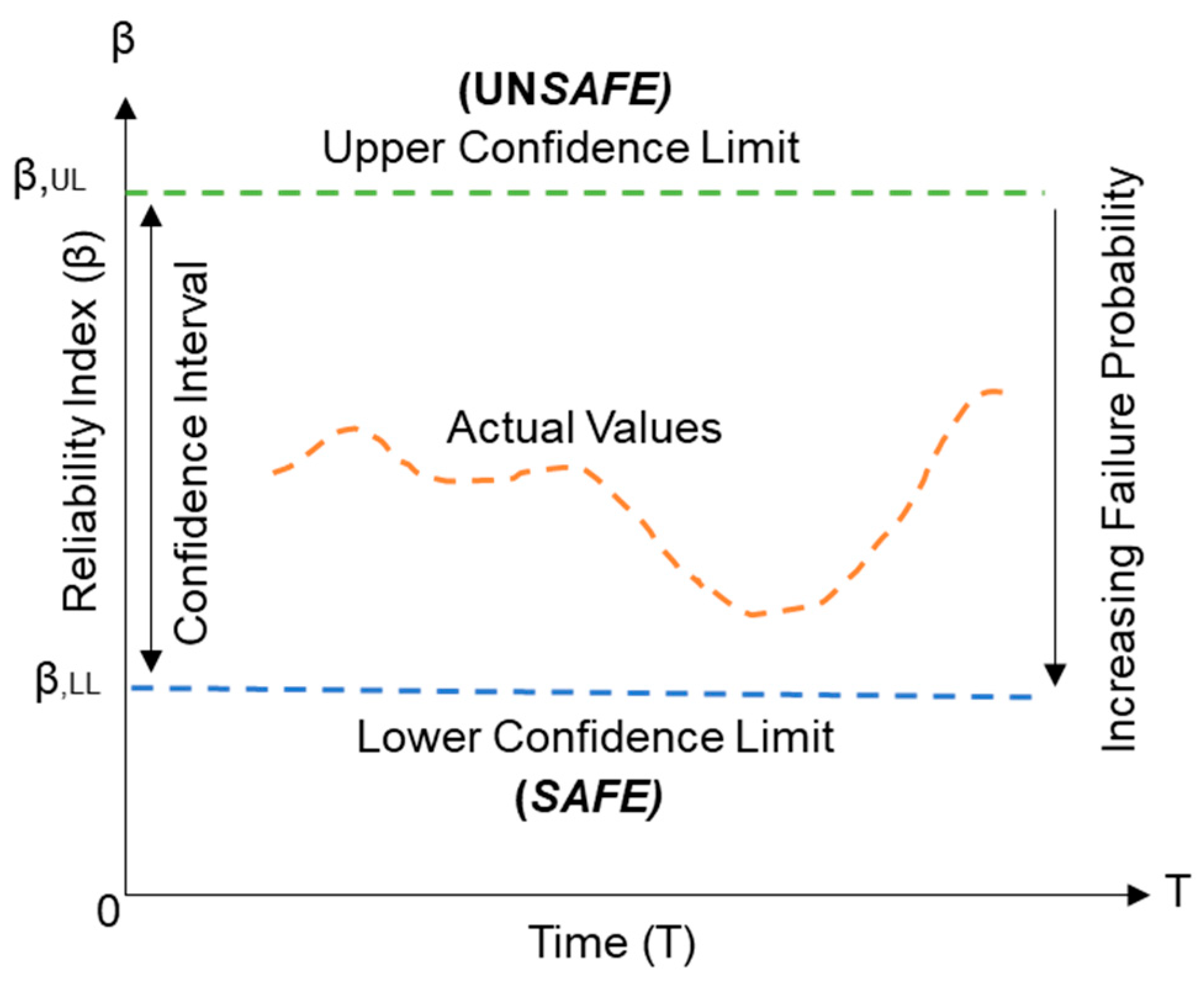
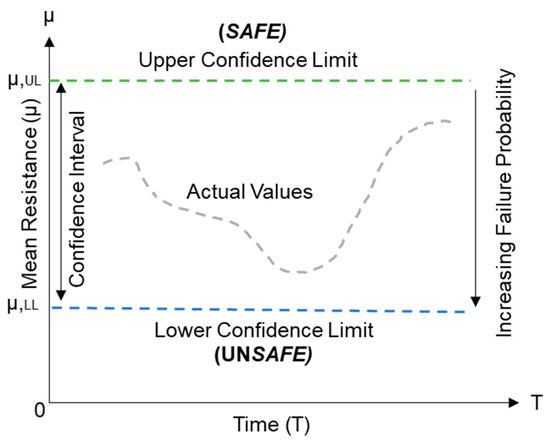
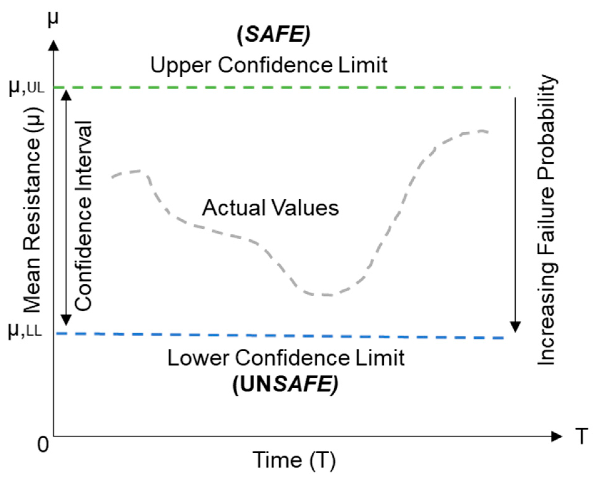
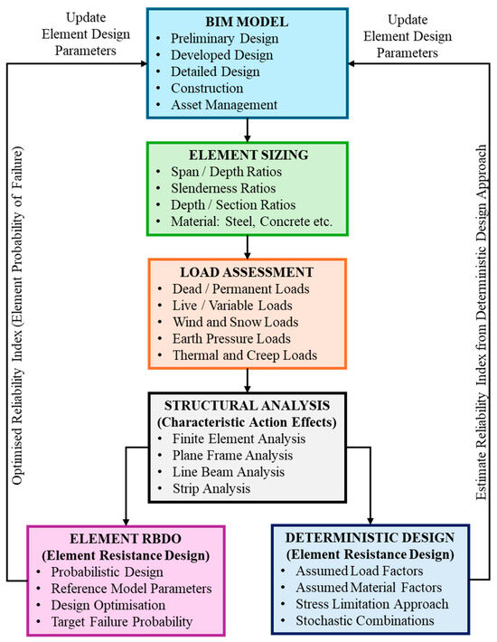
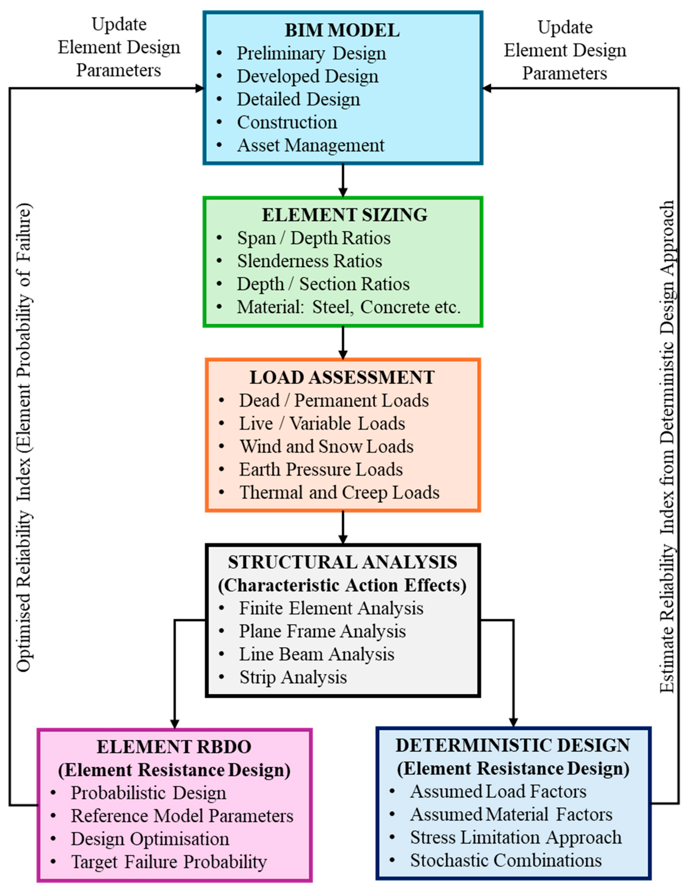
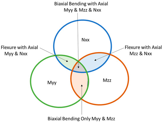
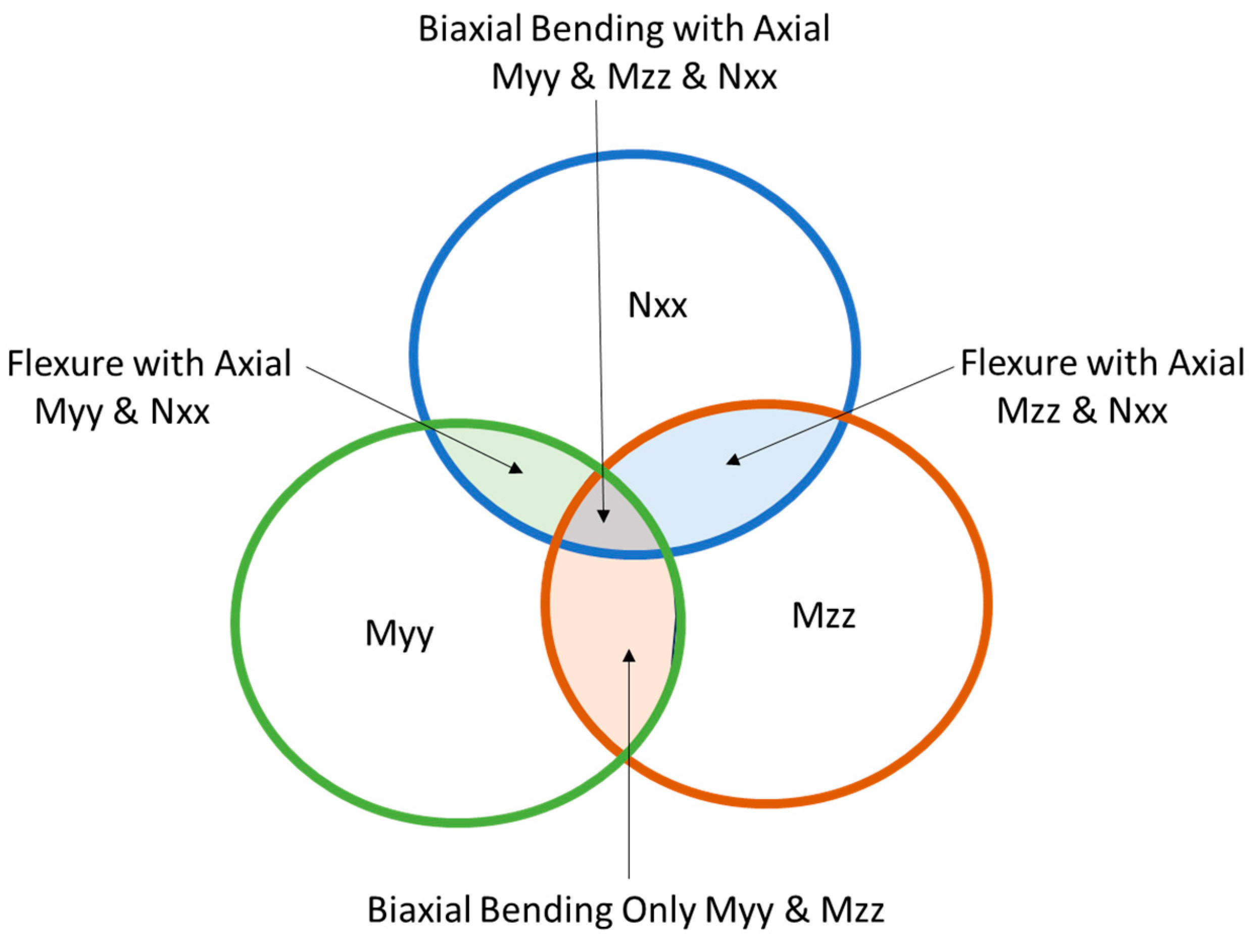
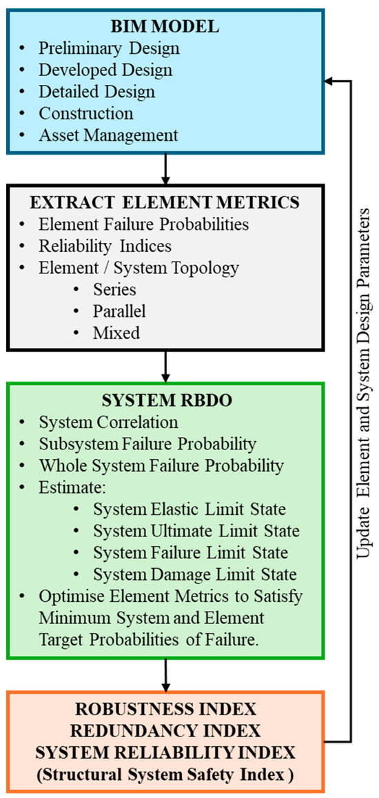
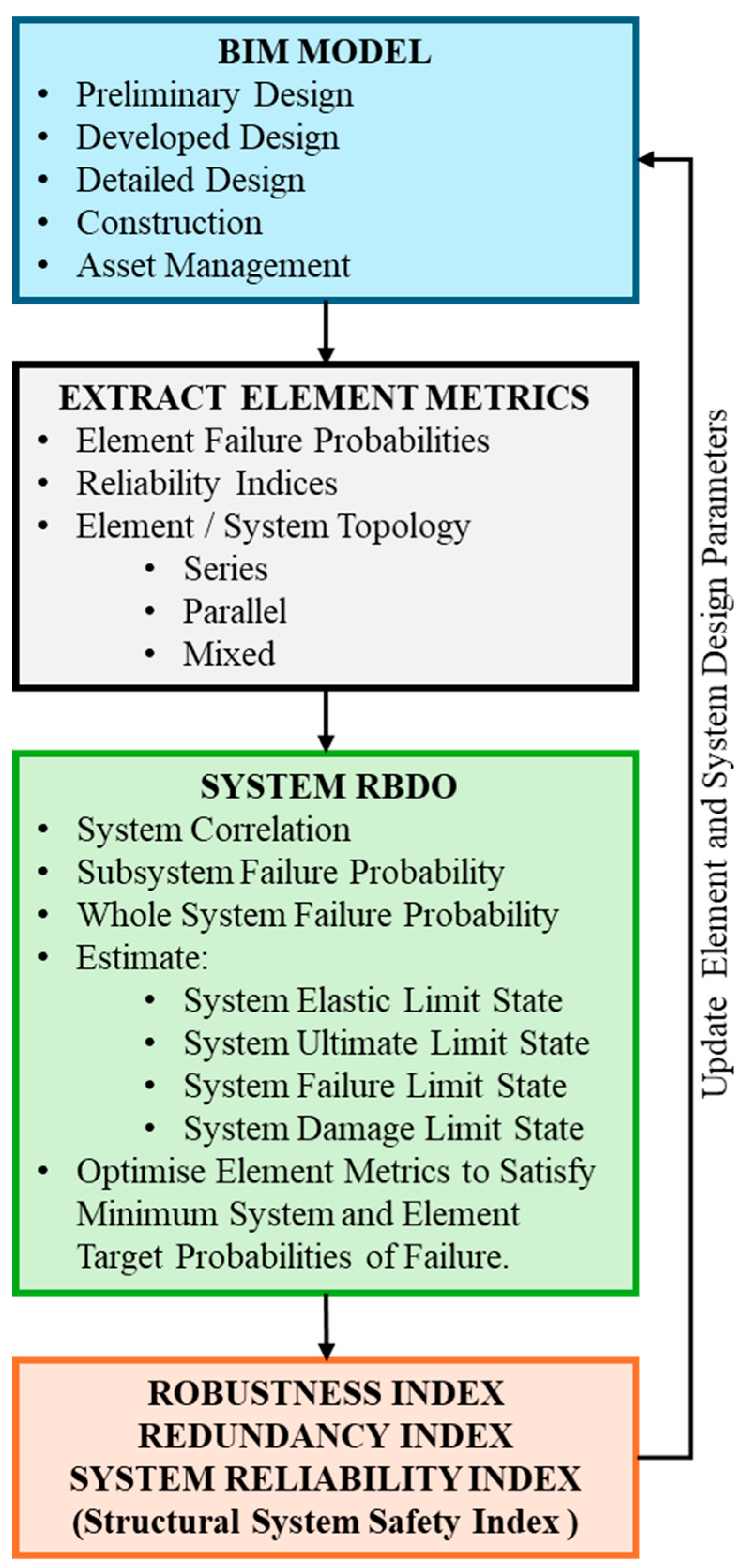
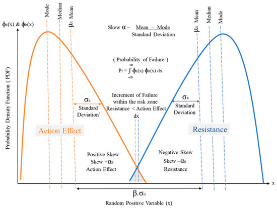
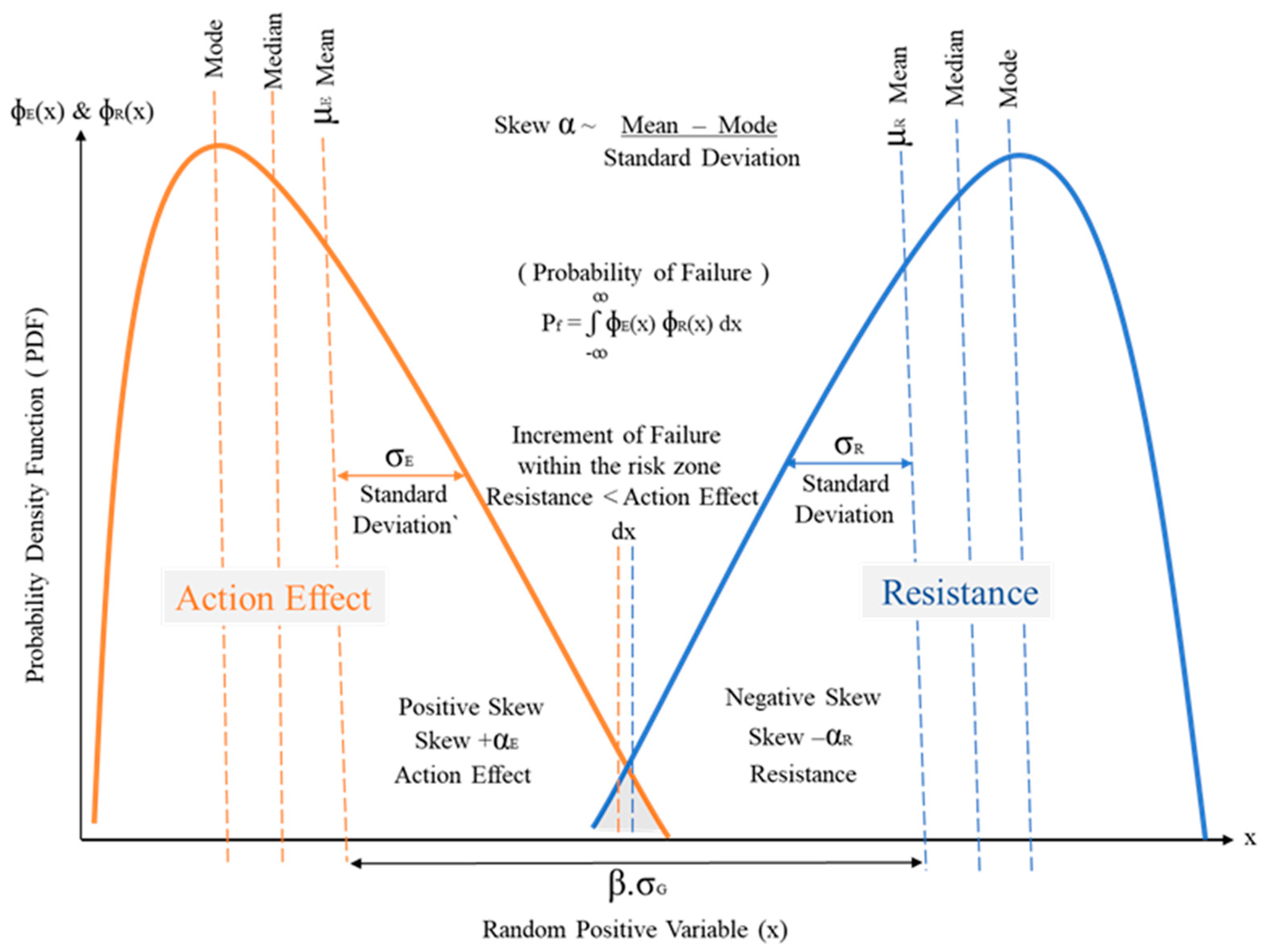
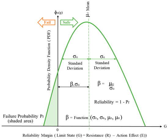
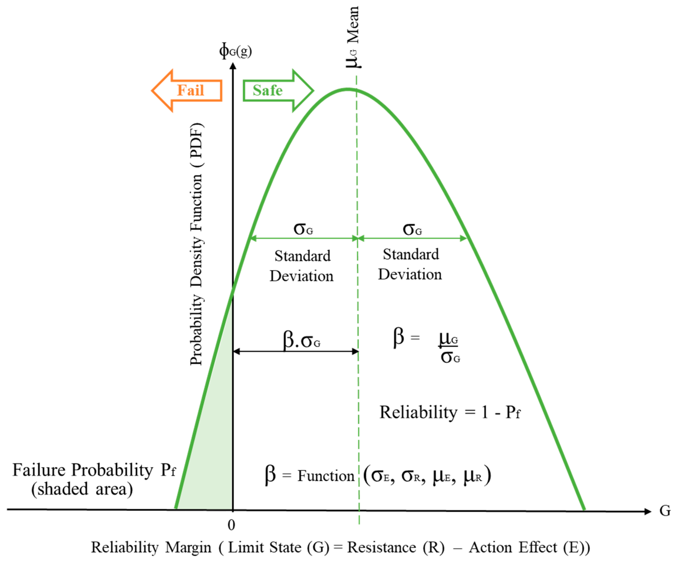
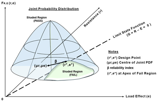
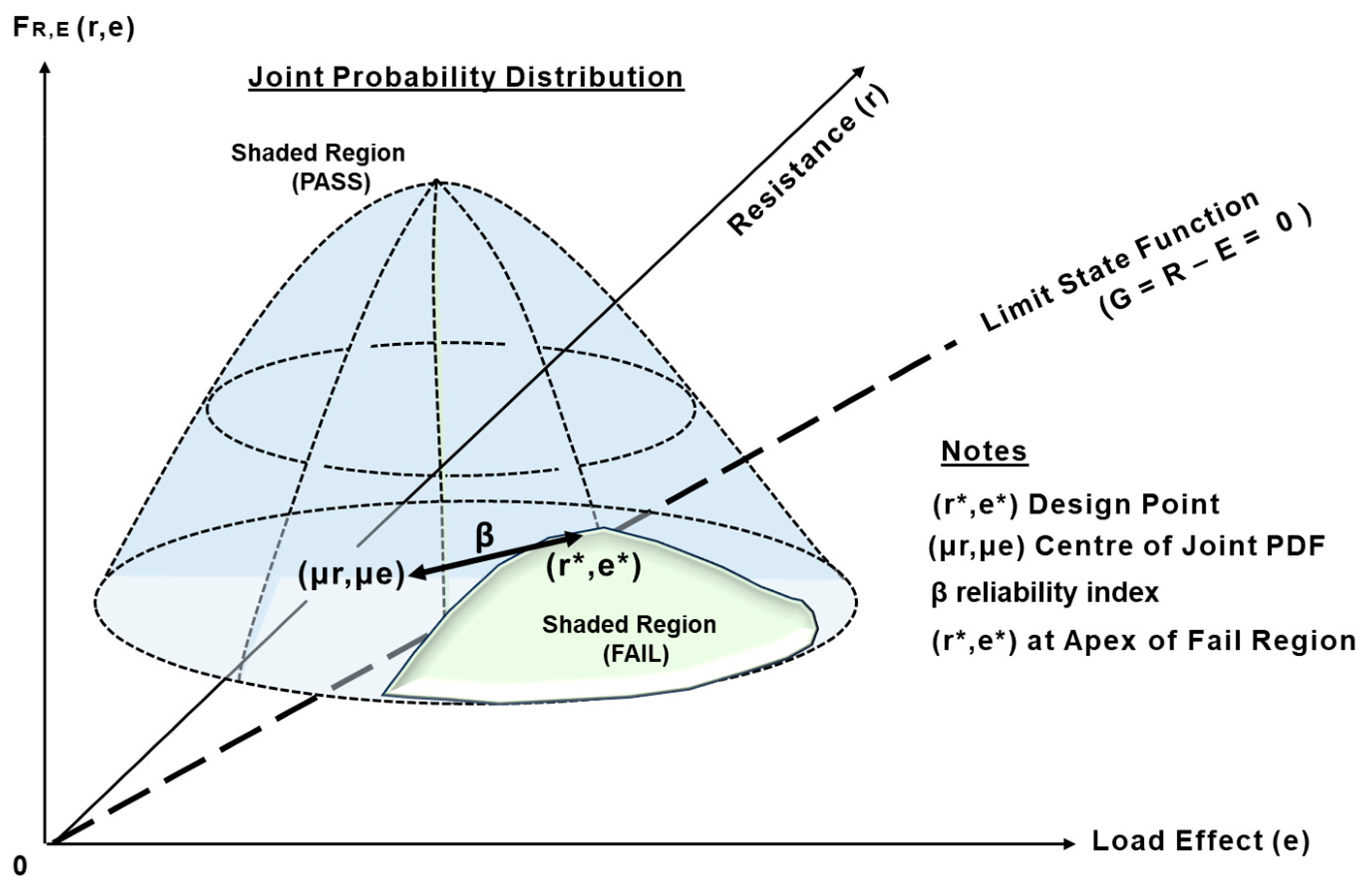
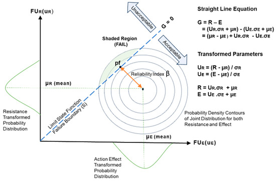
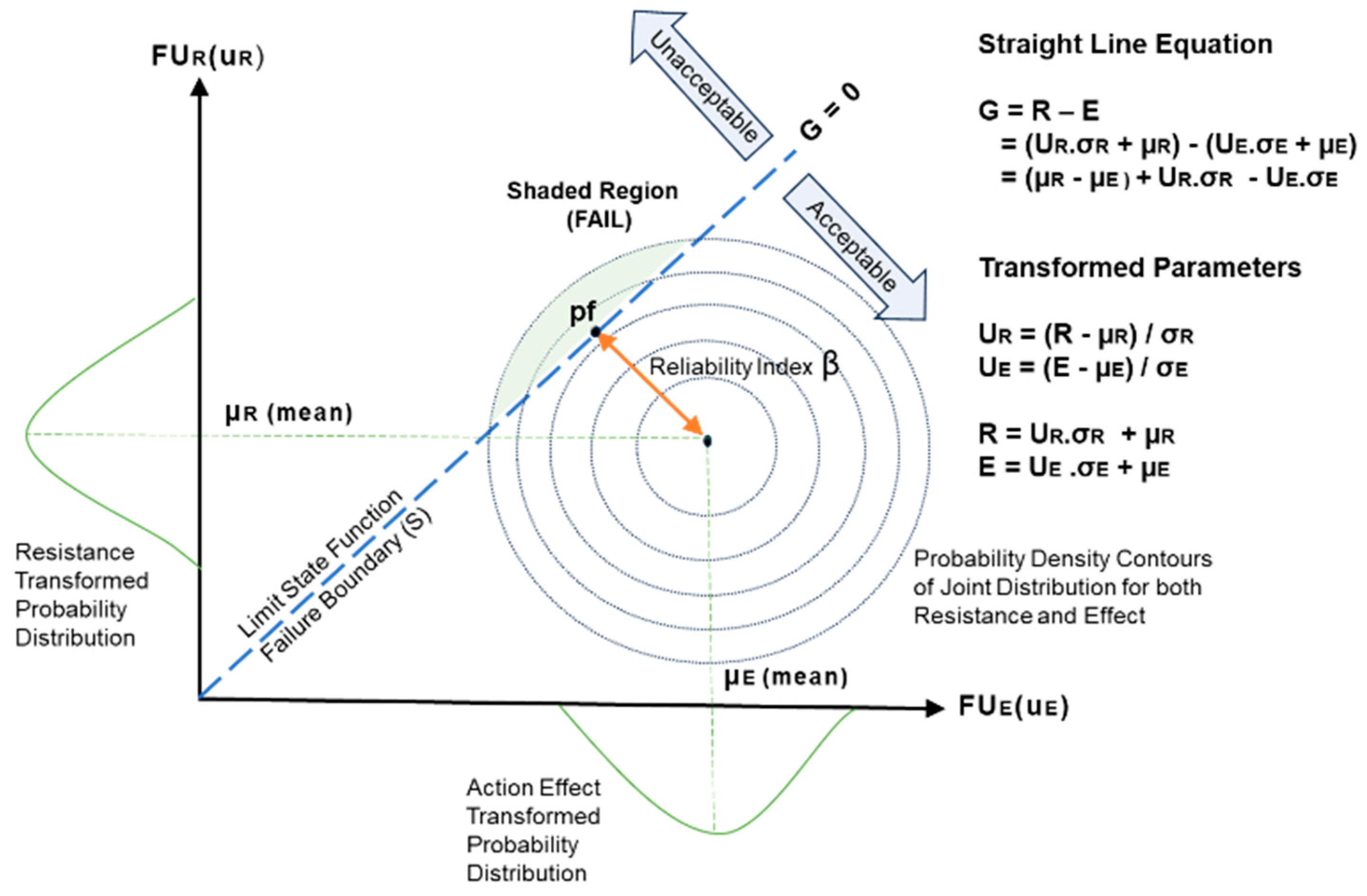
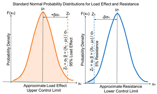
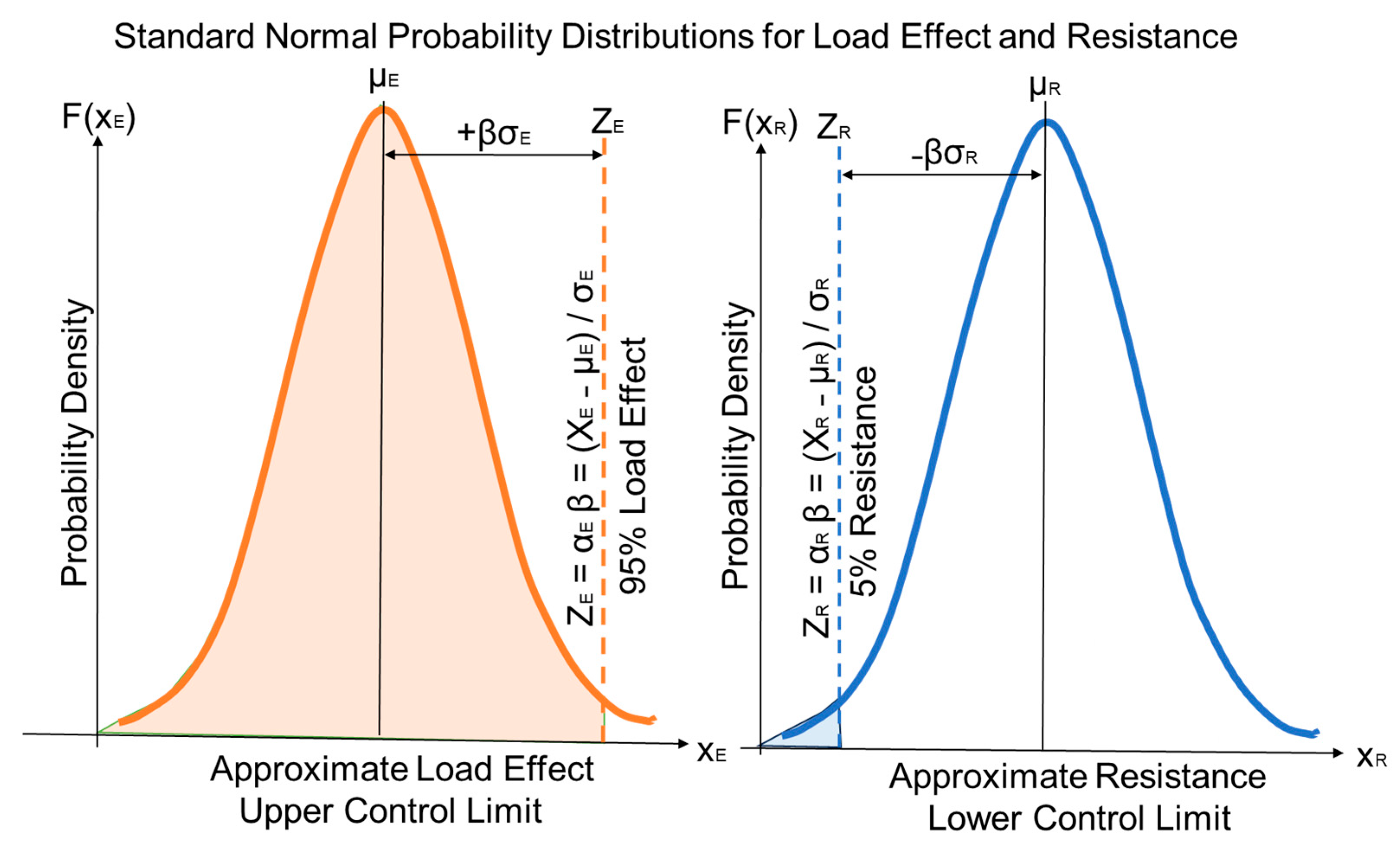
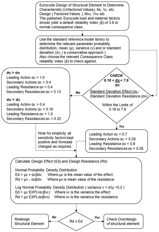
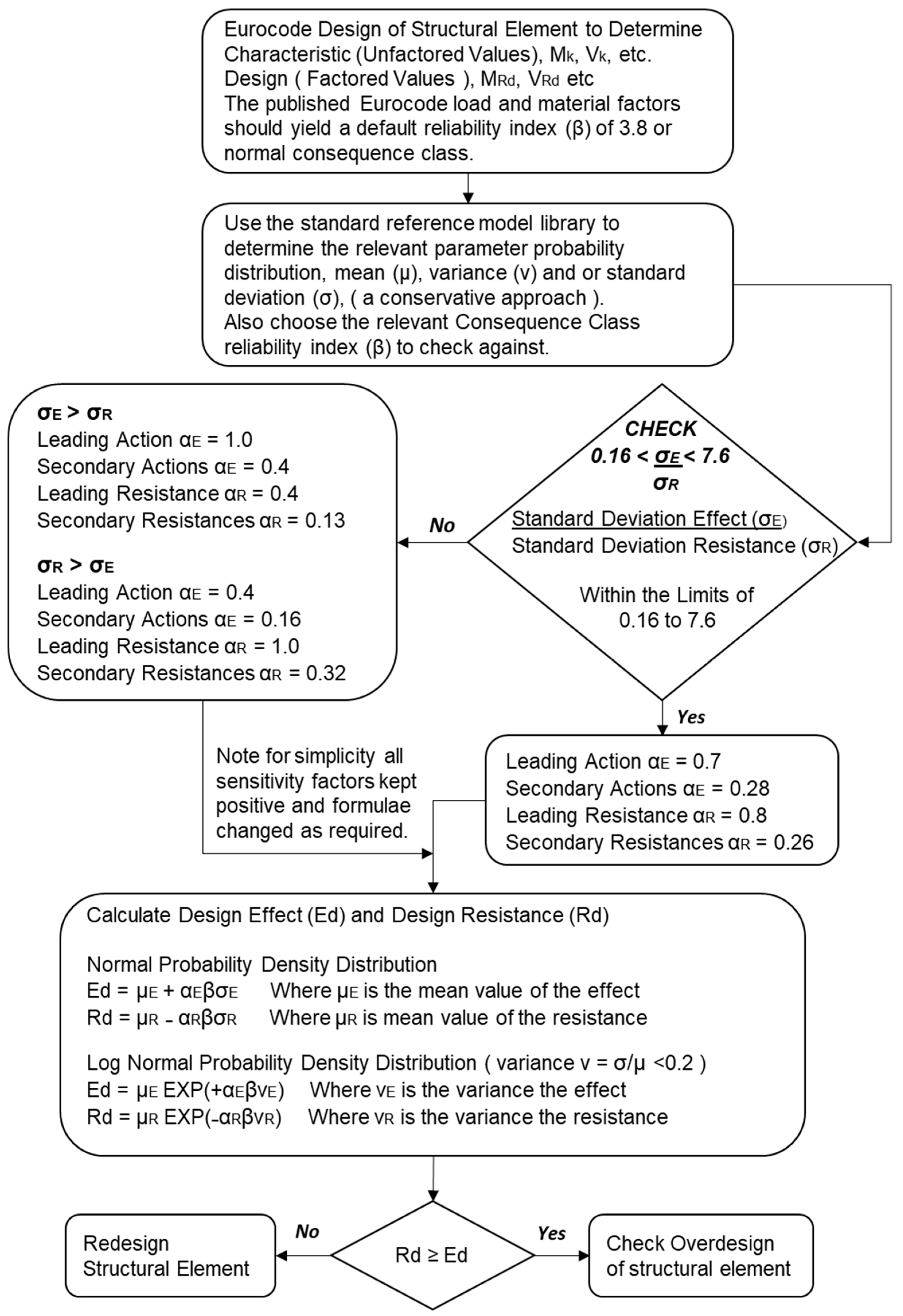
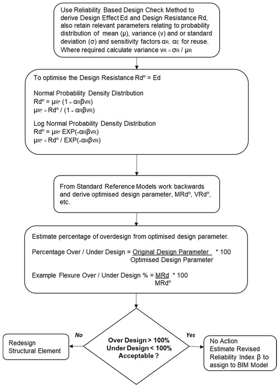
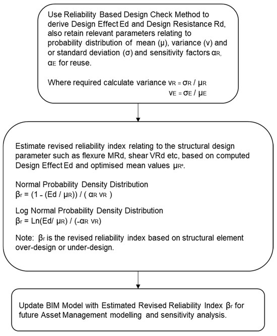
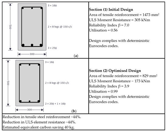
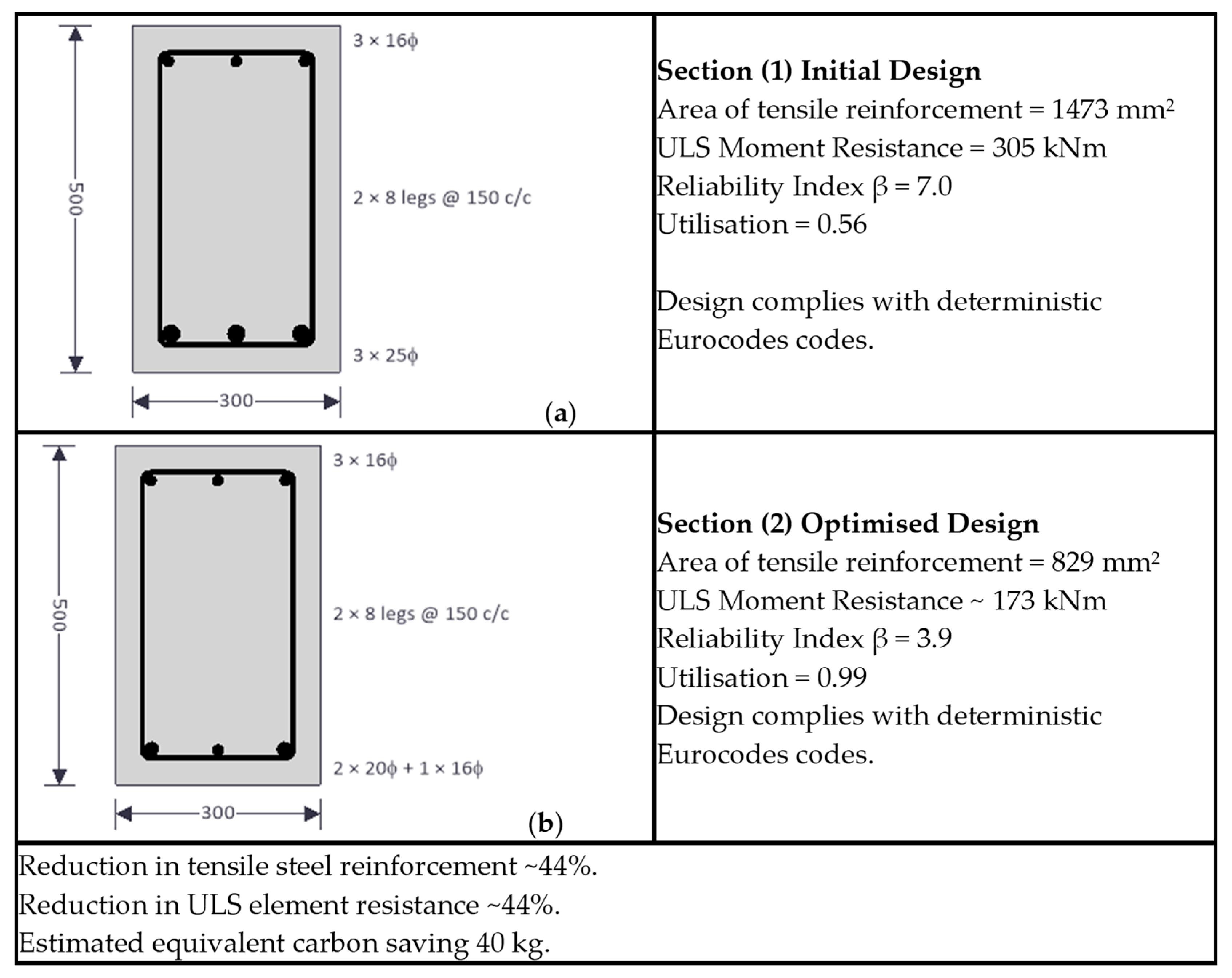
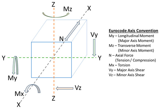
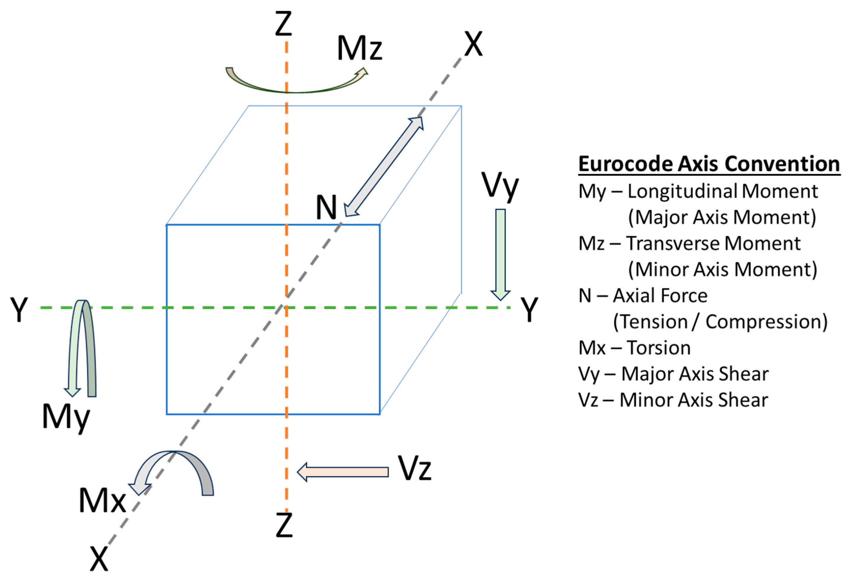
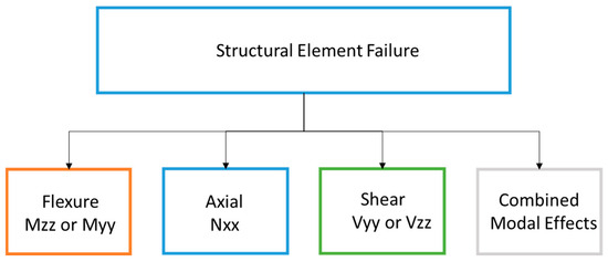
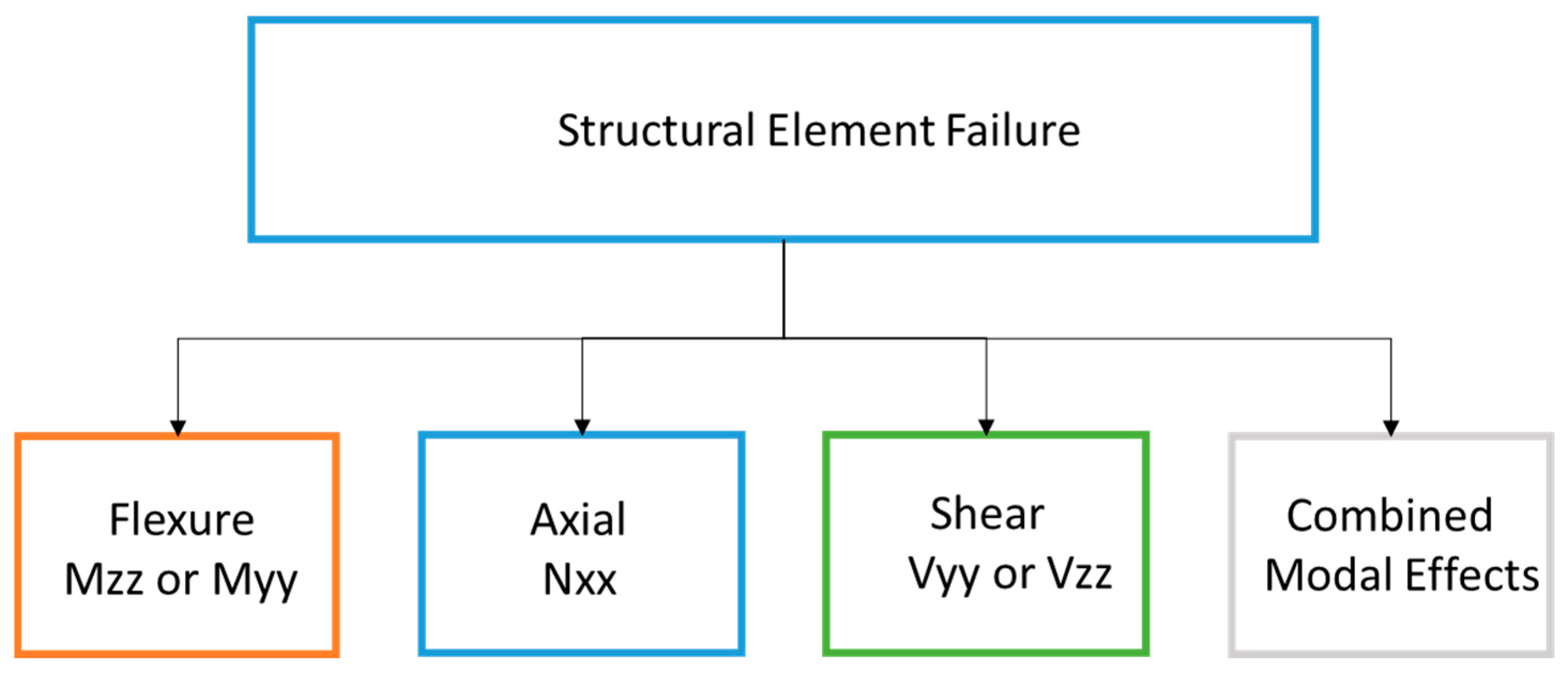
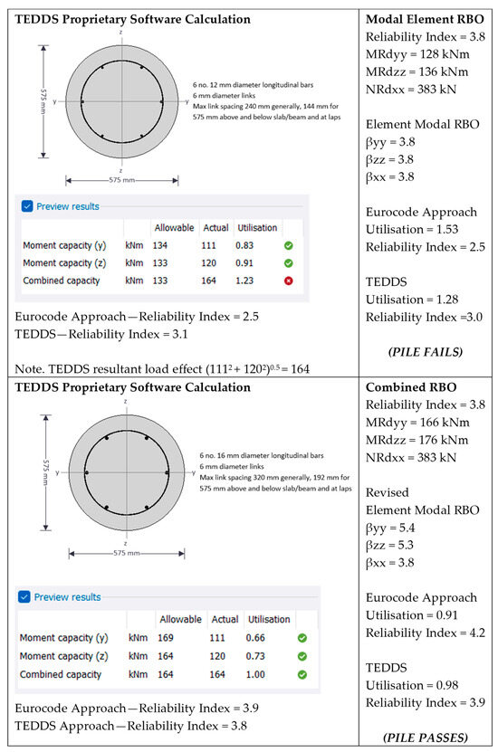
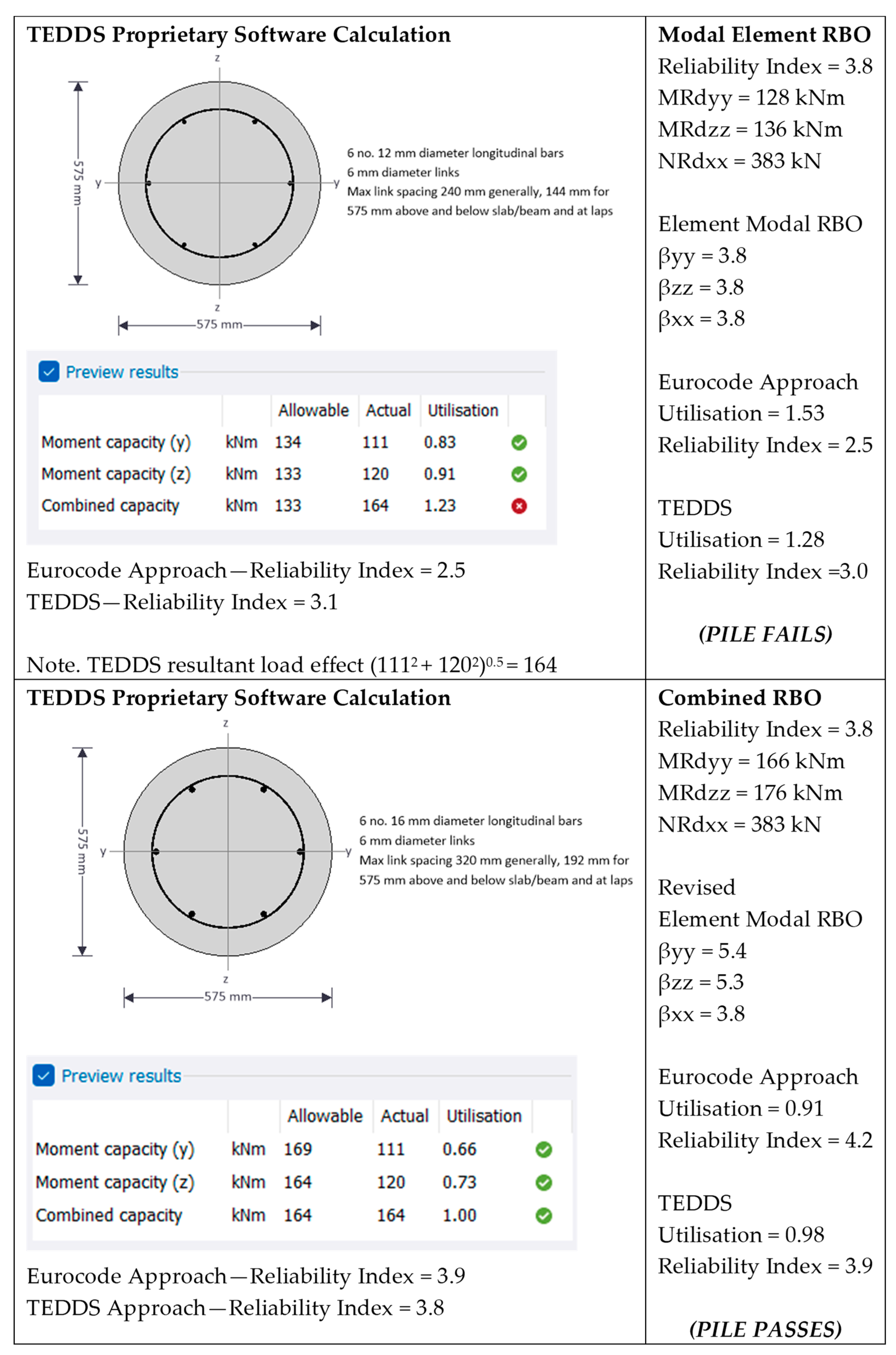
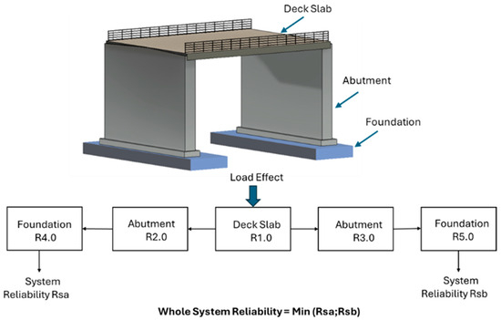
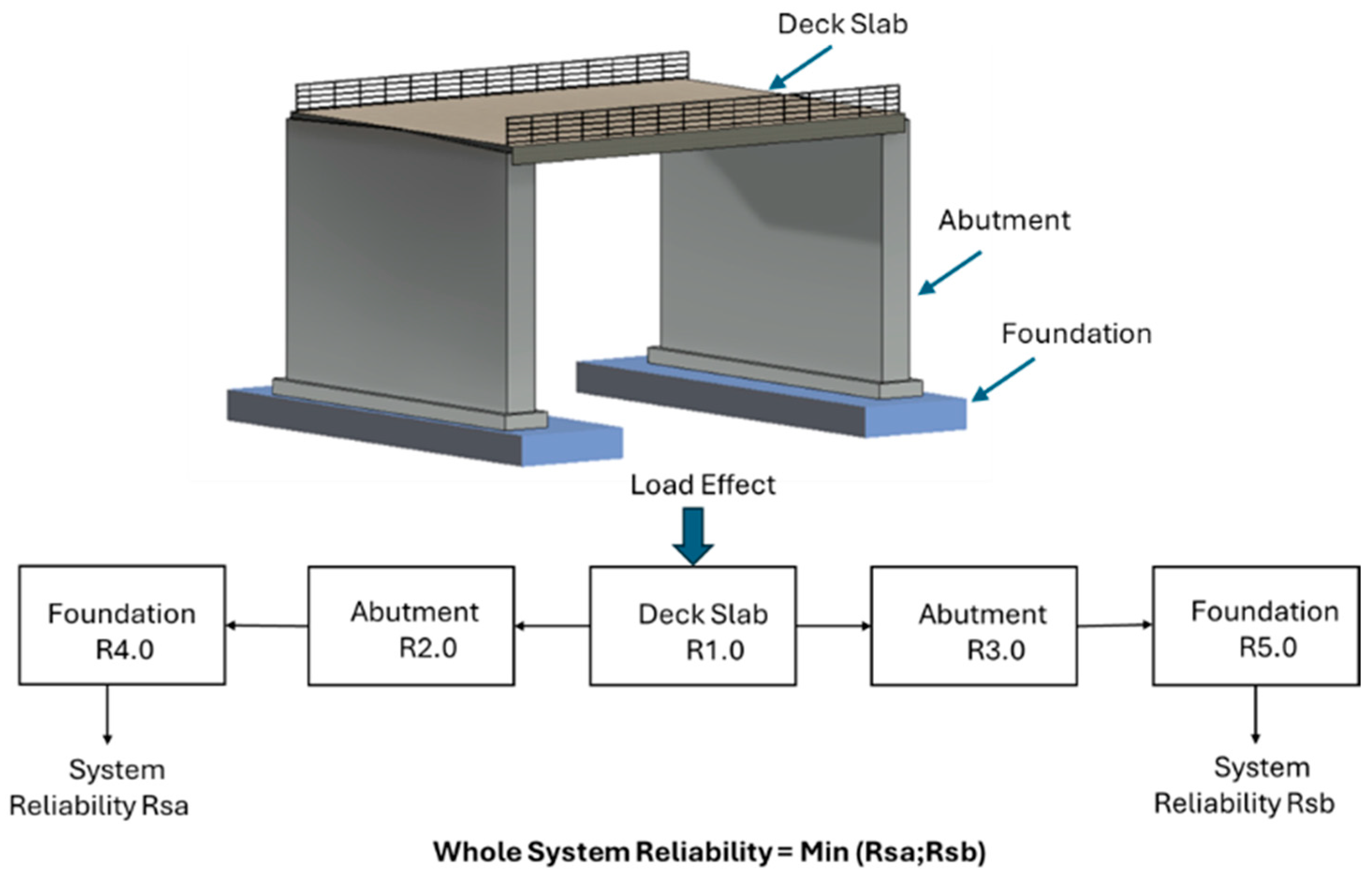
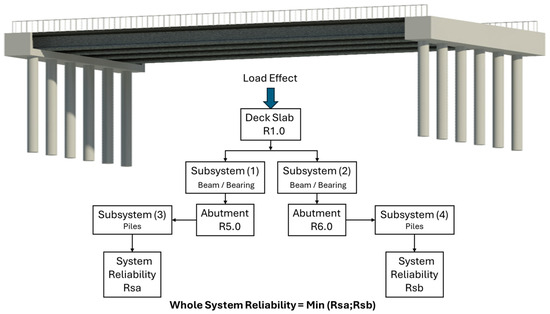
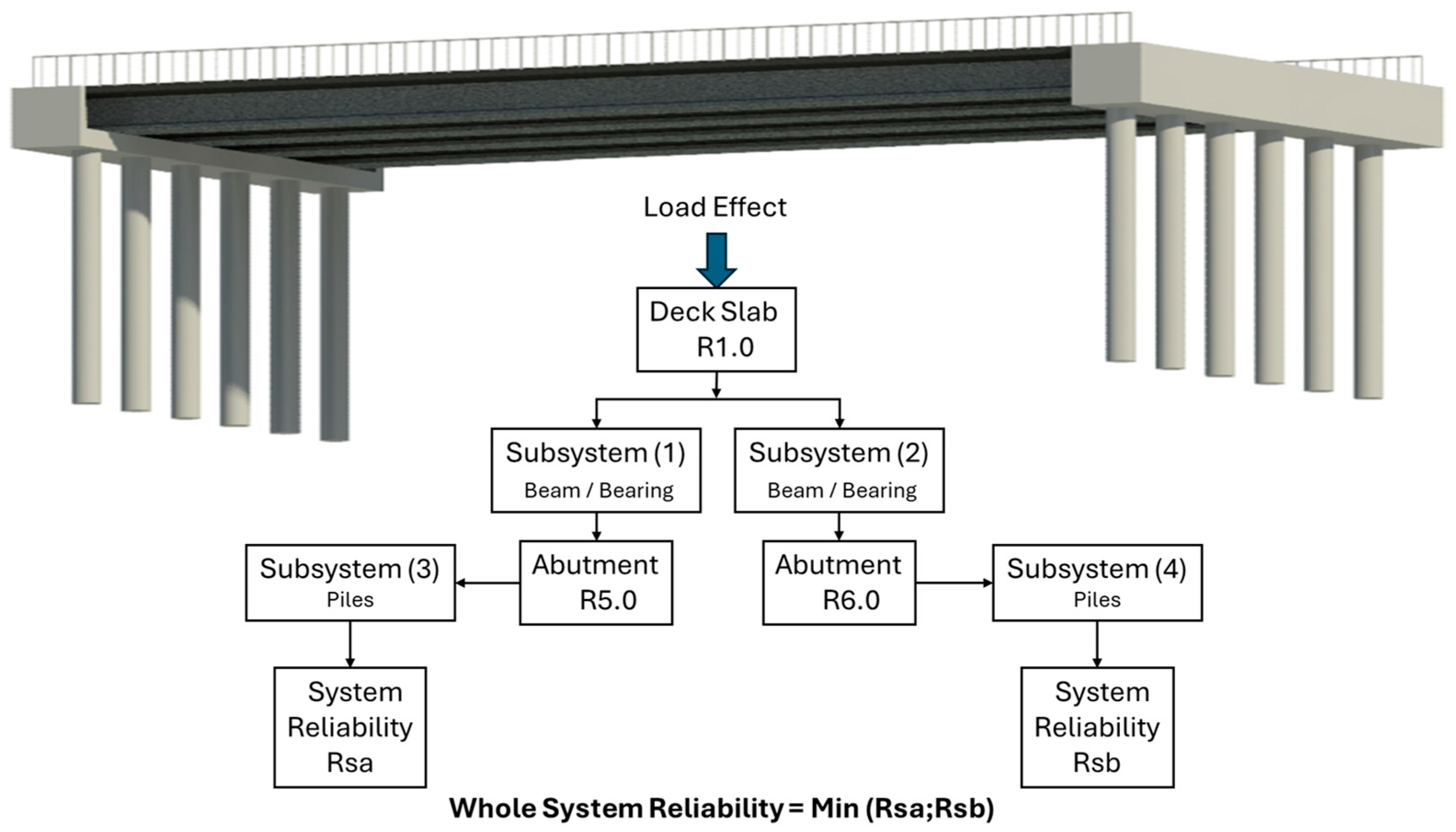
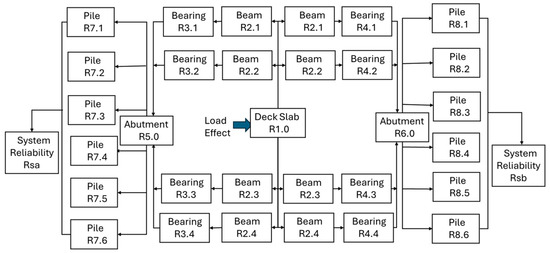
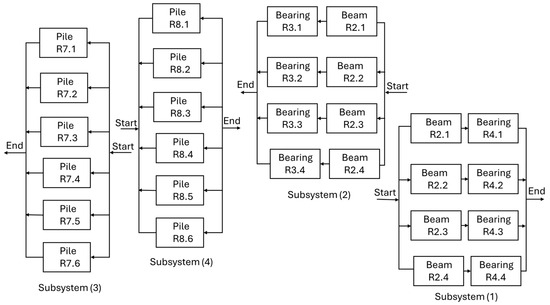
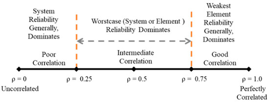
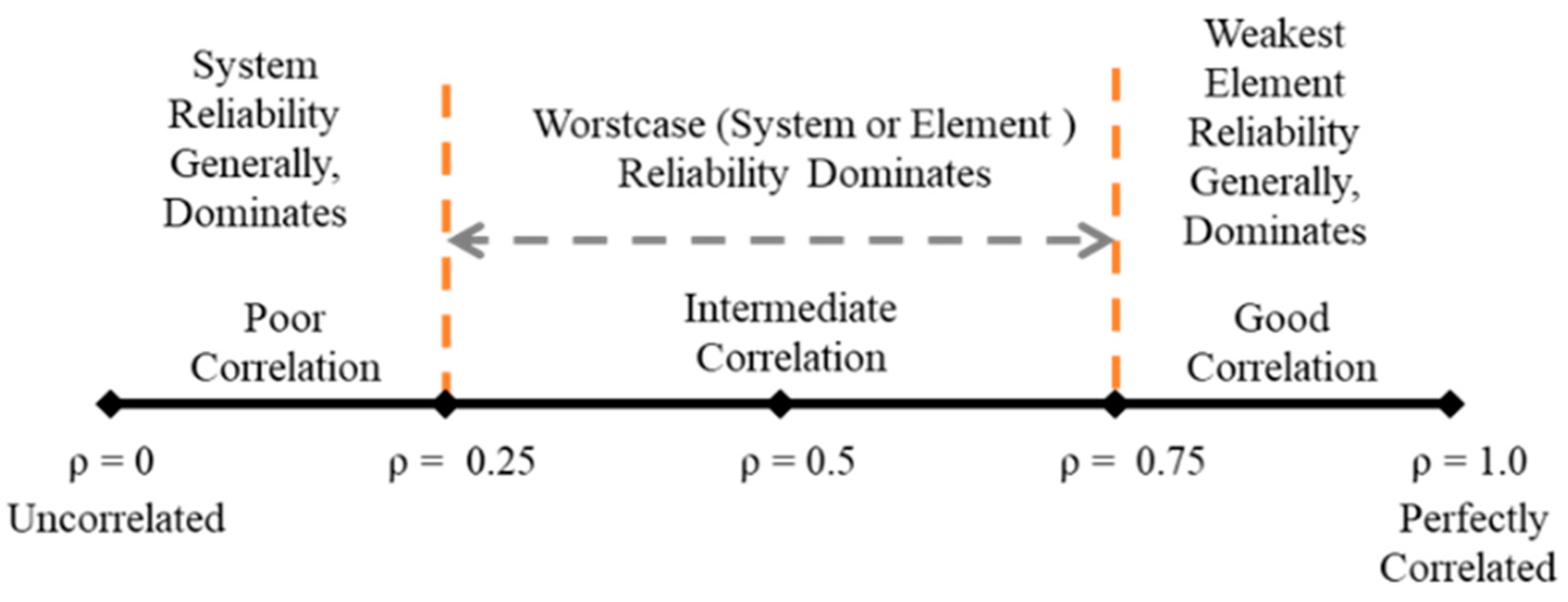
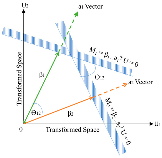
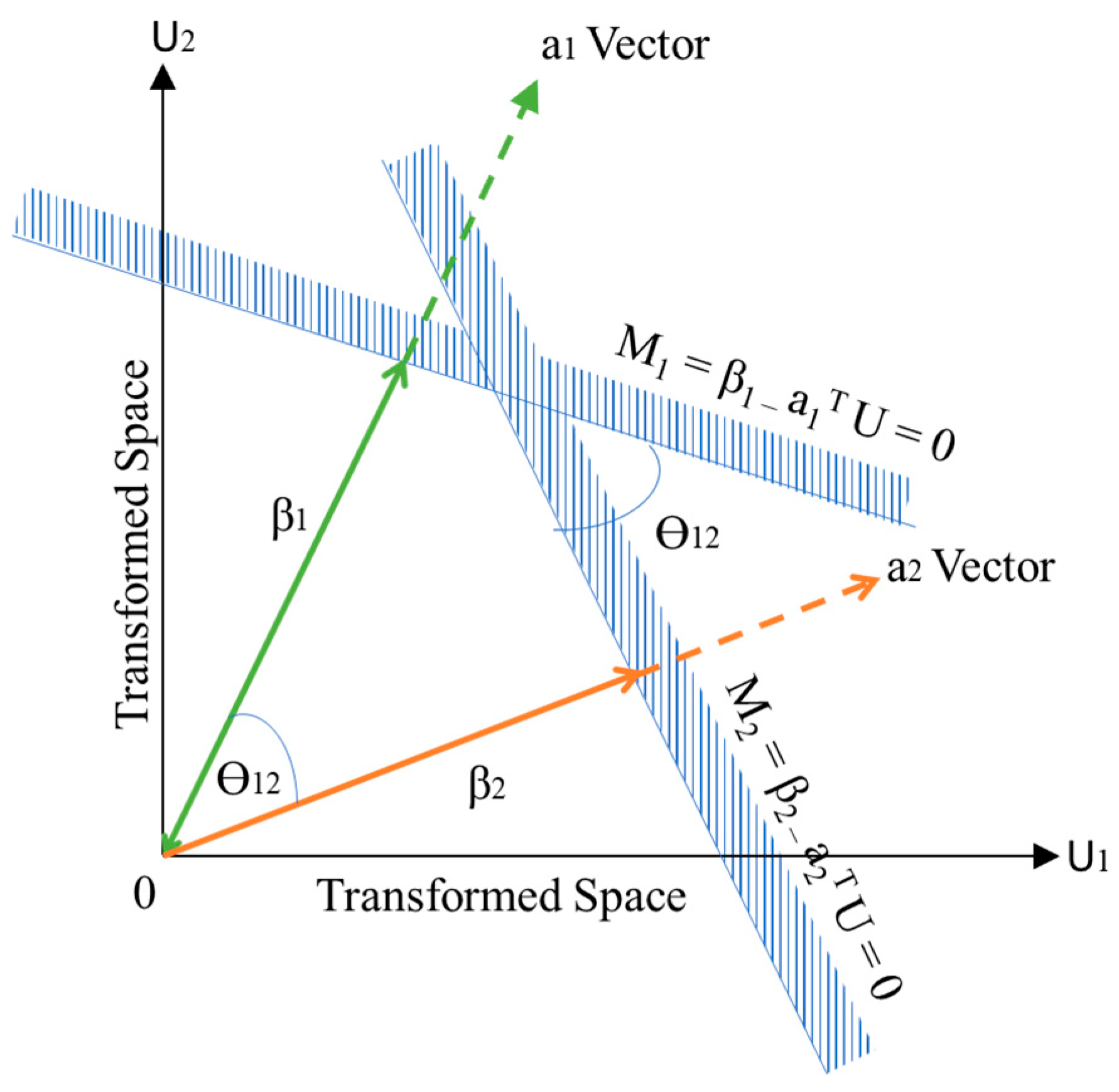
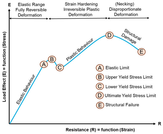
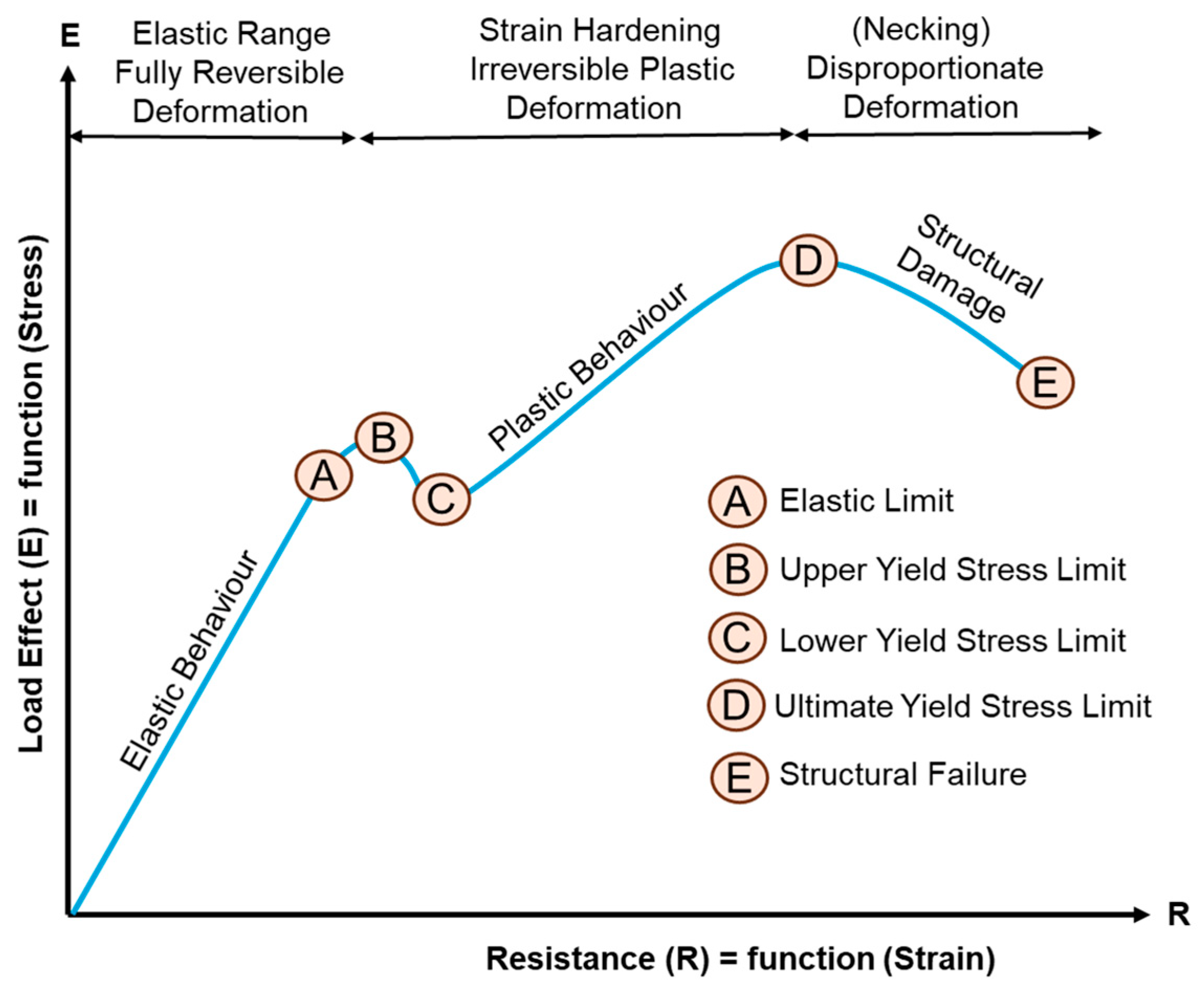
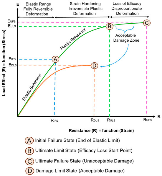
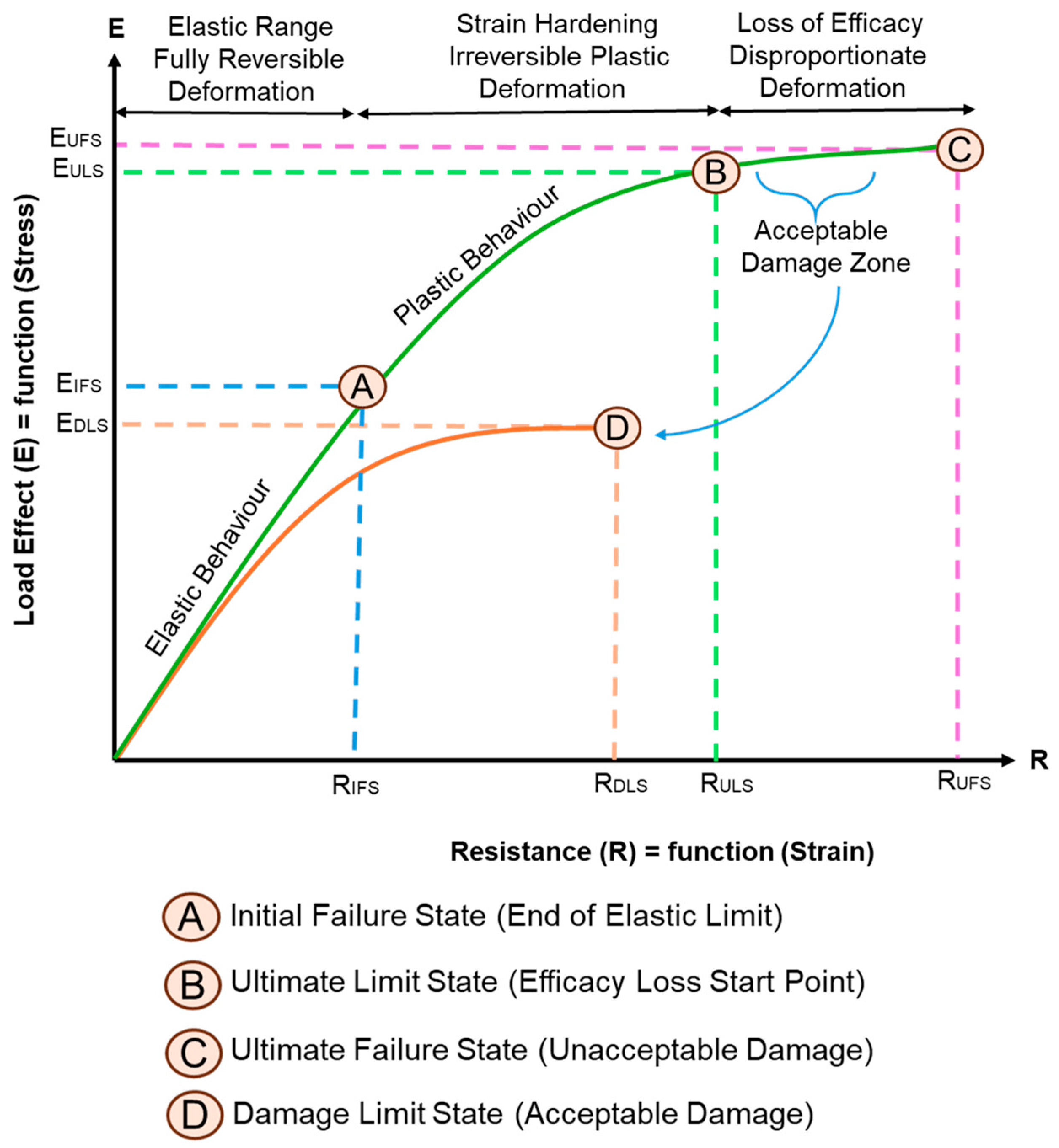
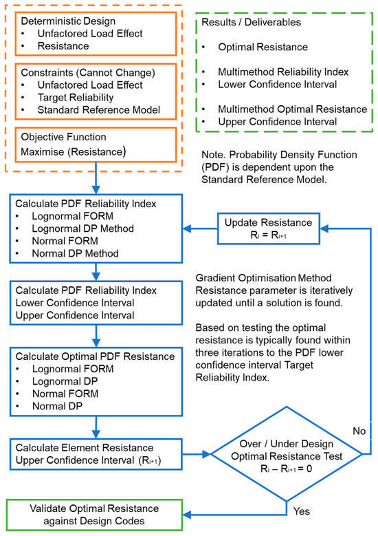
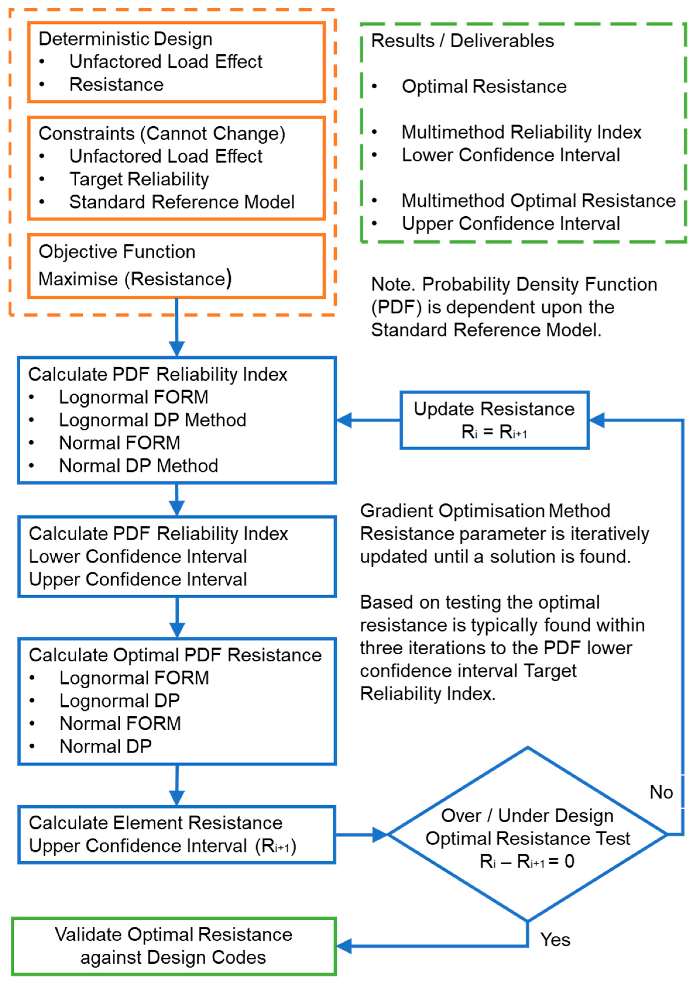
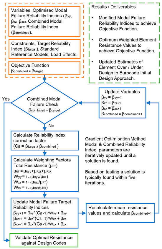
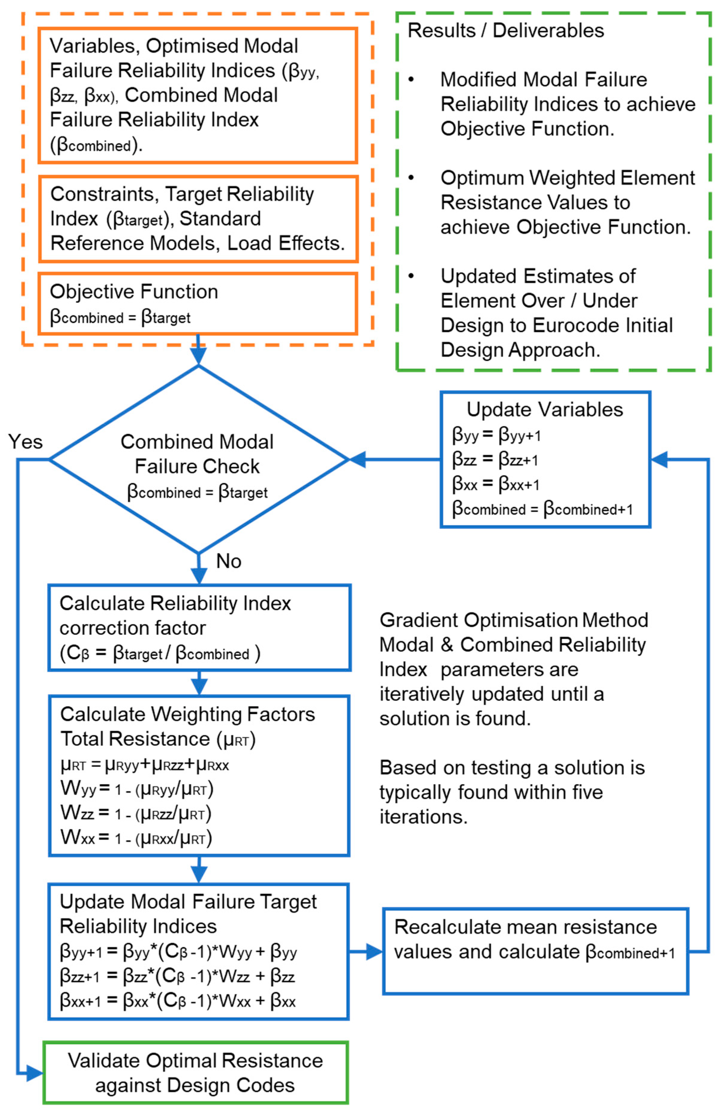
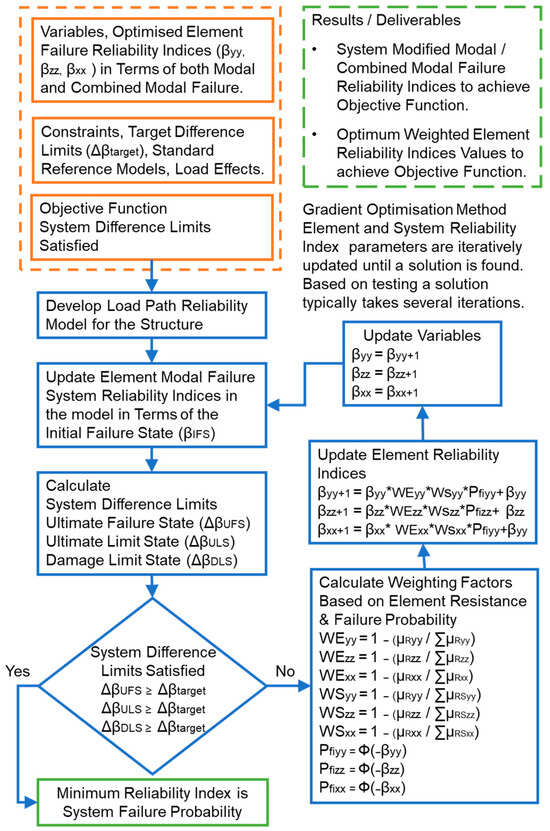
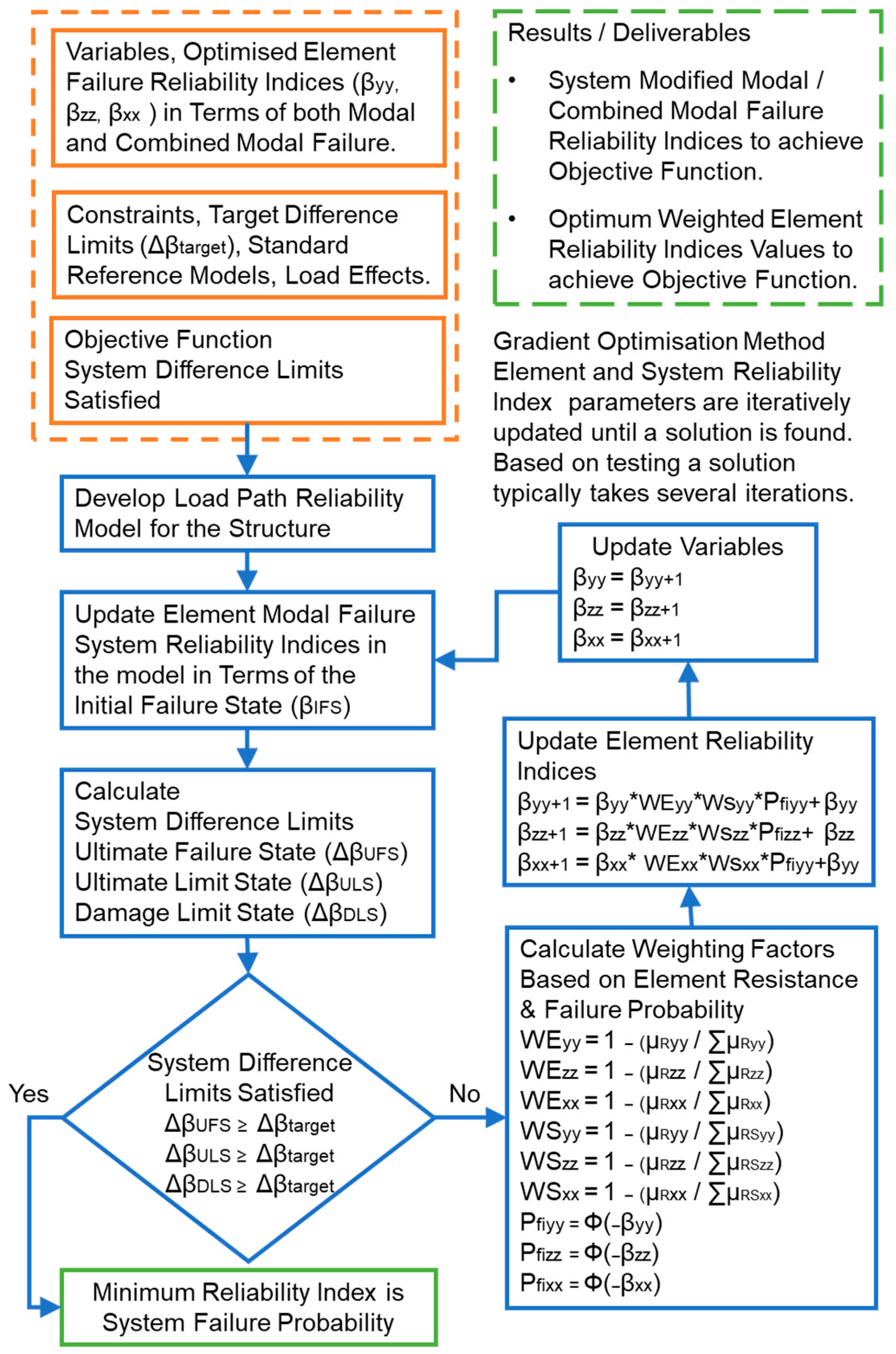
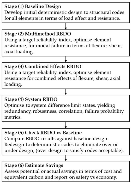
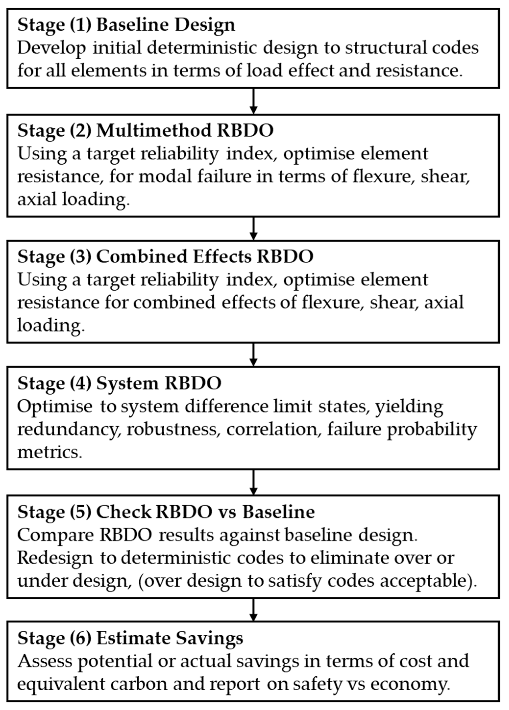
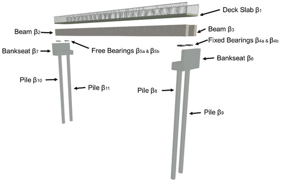
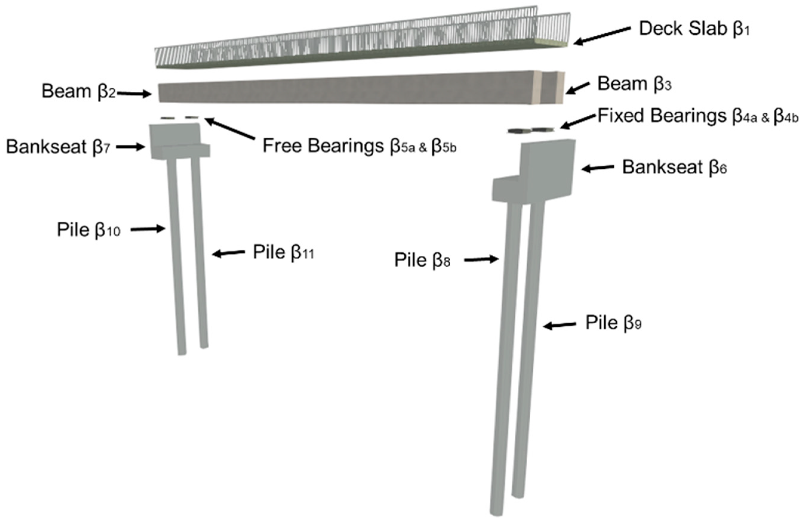
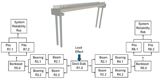
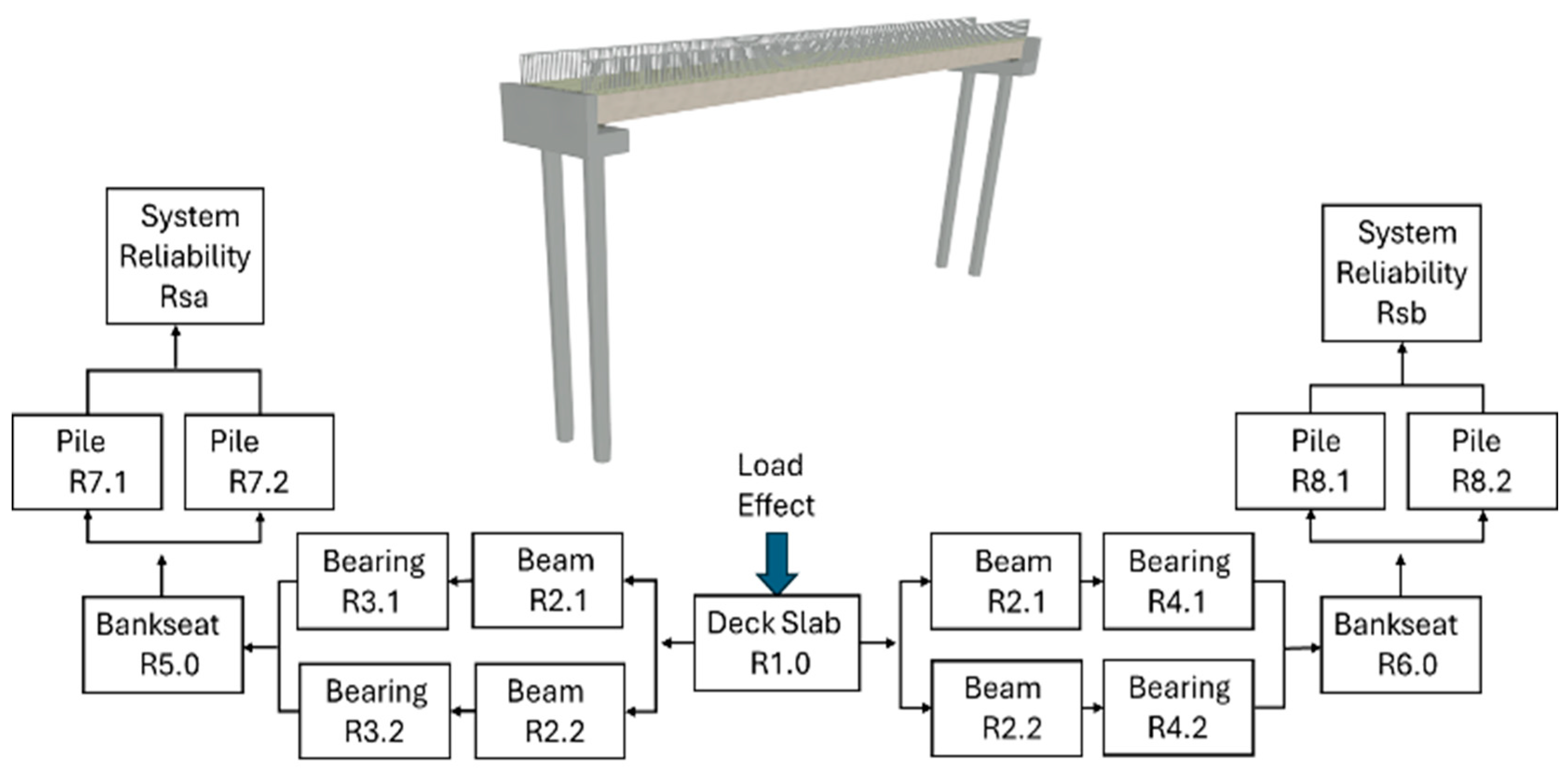
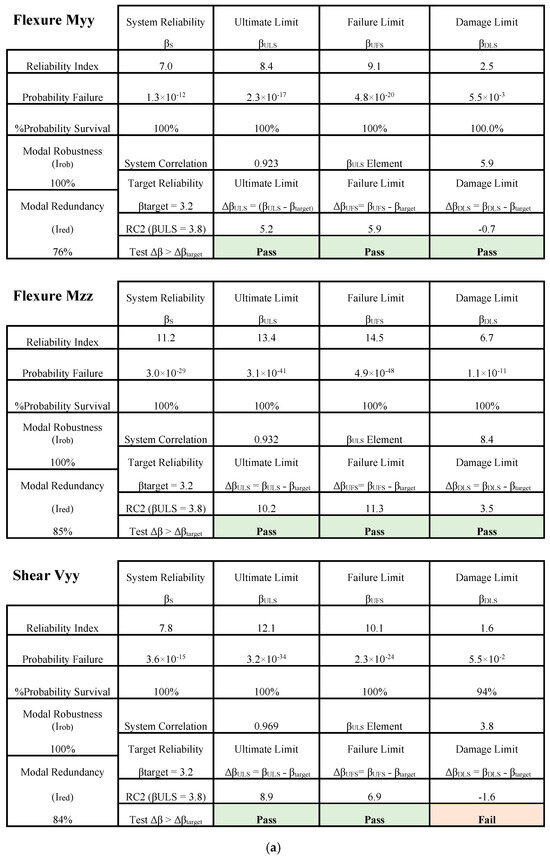
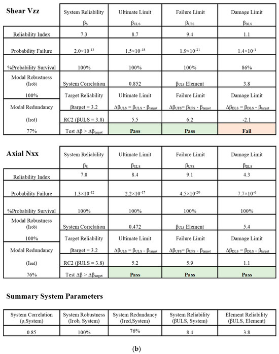
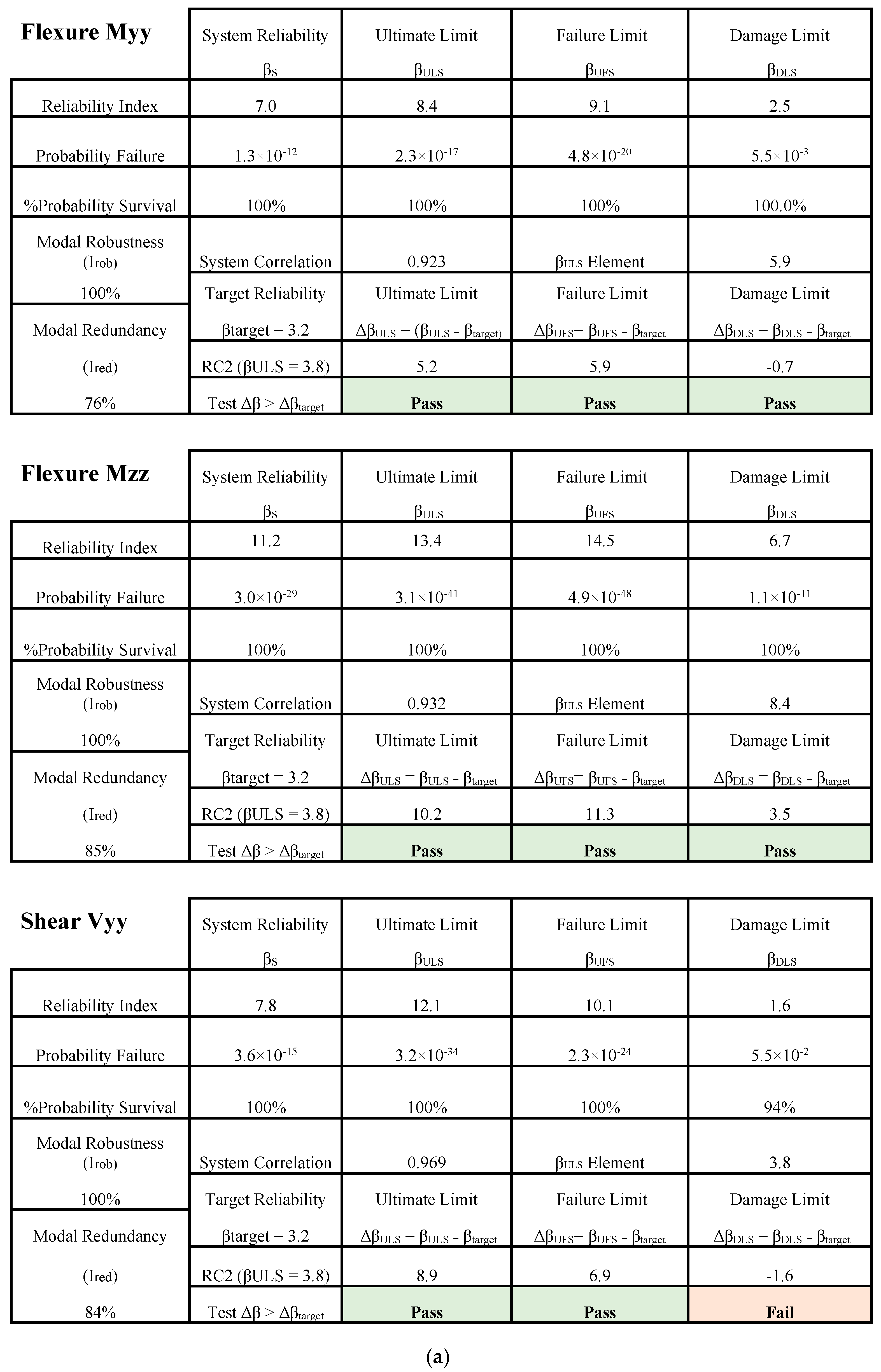
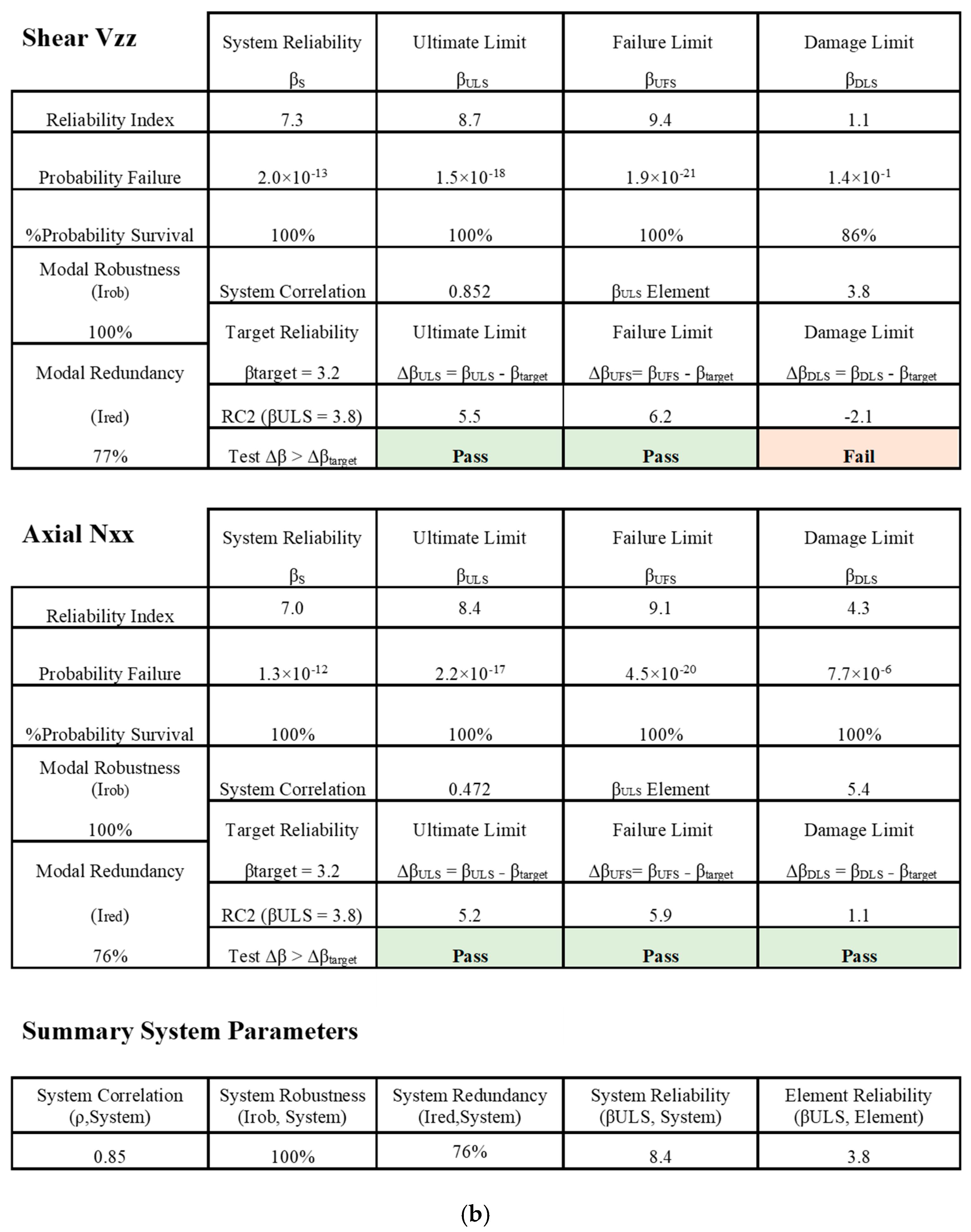
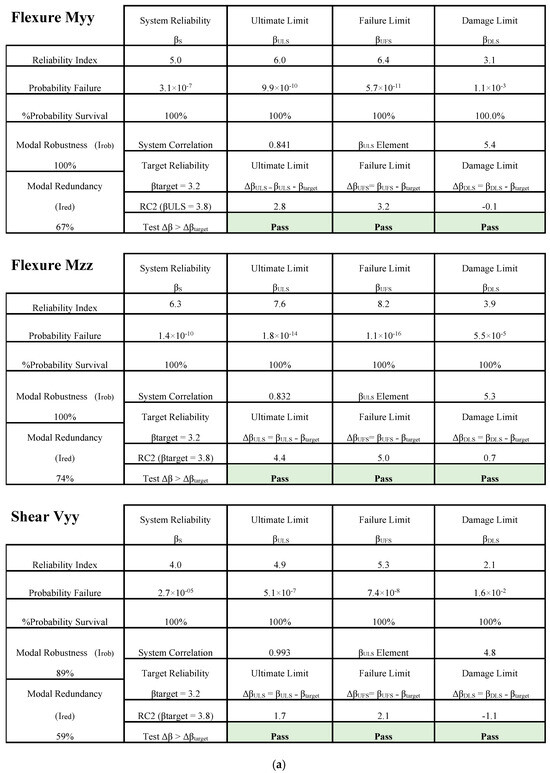
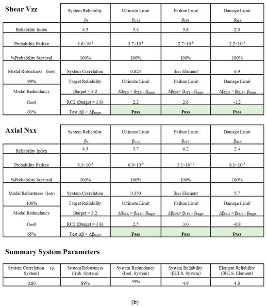
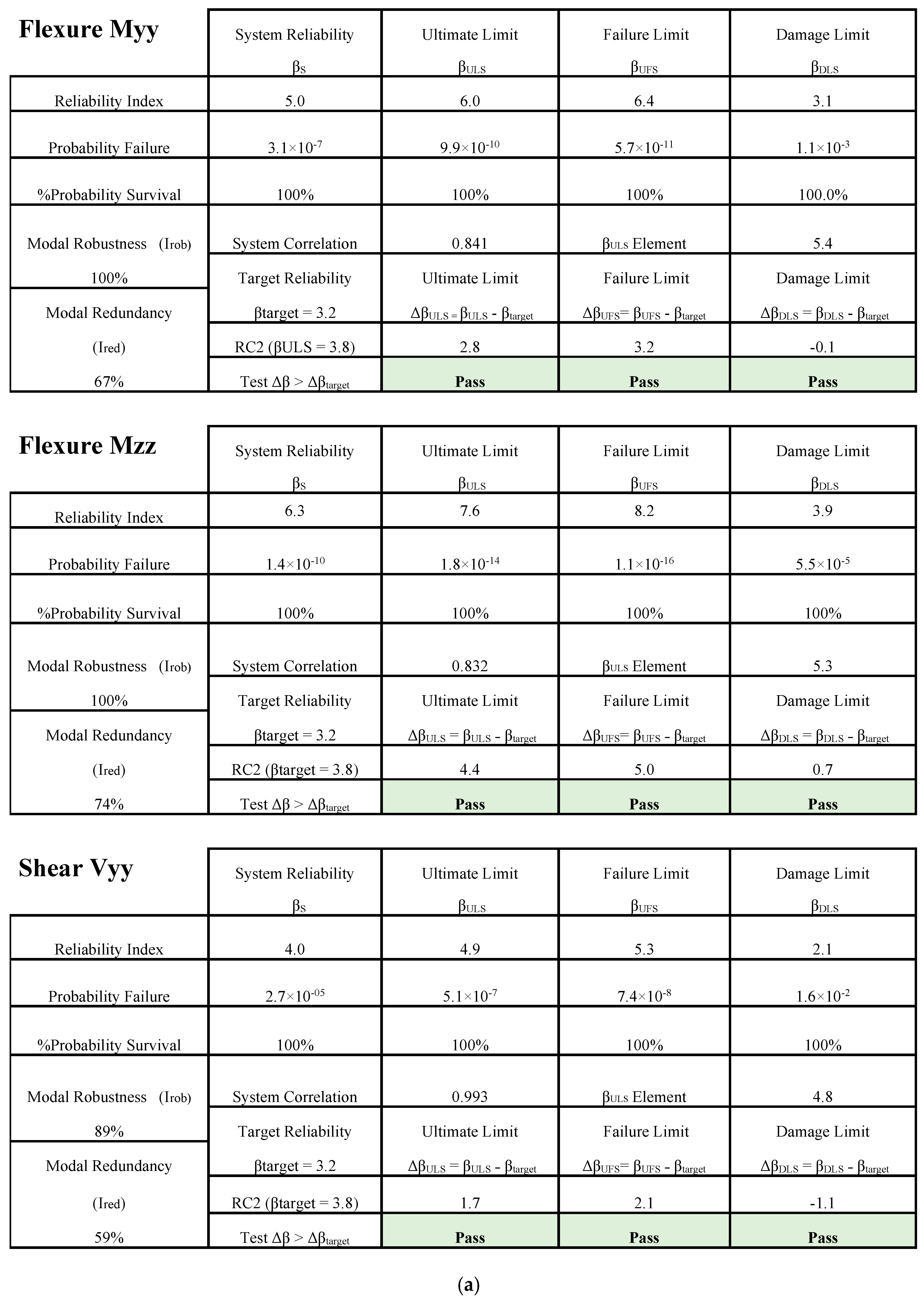
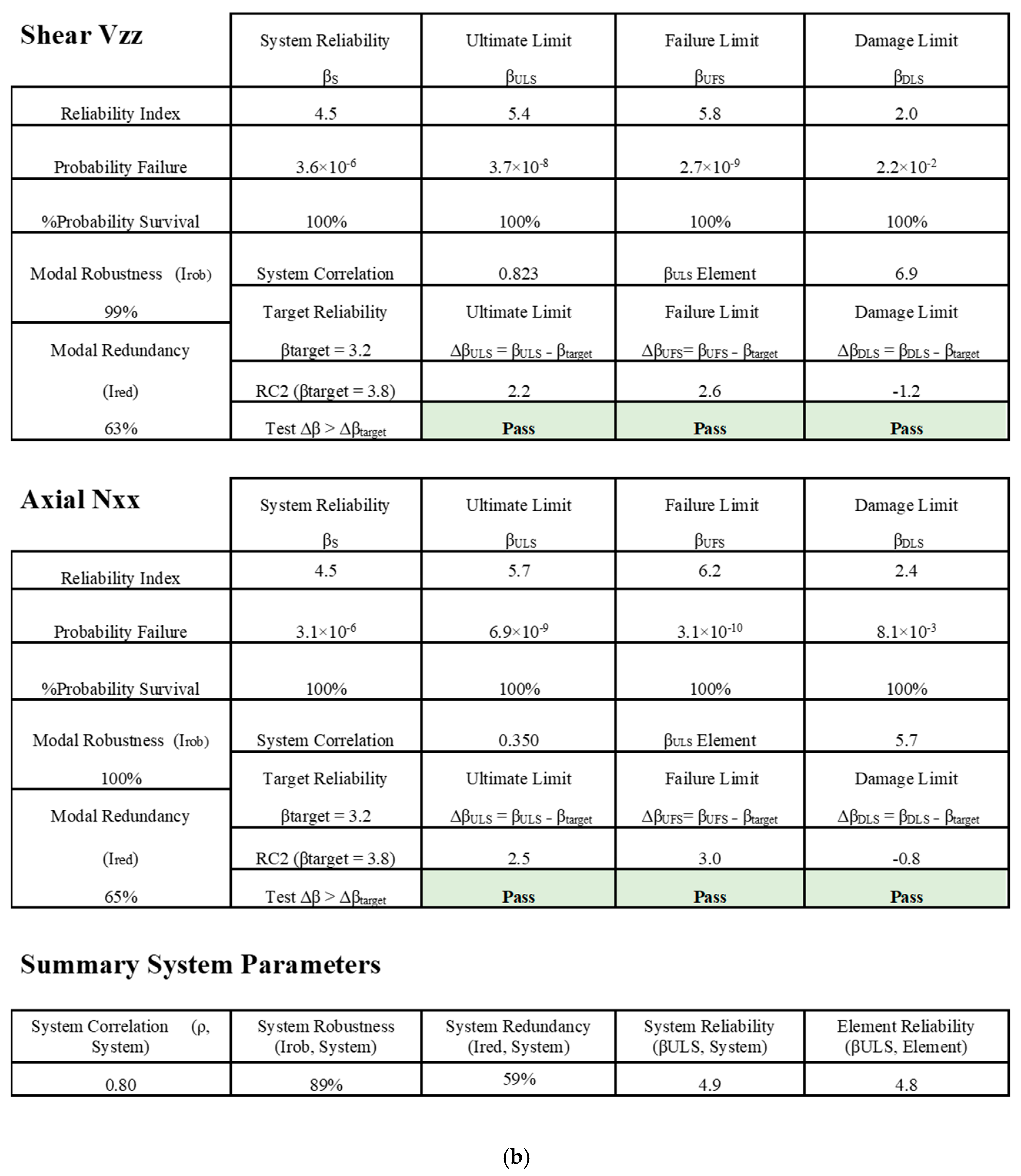

Disclaimer/Publisher’s Note: The statements, opinions and data contained in all publications are solely those of the individual author(s) and contributor(s) and not of MDPI and/or the editor(s). MDPI and/or the editor(s) disclaim responsibility for any injury to people or property resulting from any ideas, methods, instructions or products referred to in the content. |
© 2026 by the authors. Licensee MDPI, Basel, Switzerland. This article is an open access article distributed under the terms and conditions of the Creative Commons Attribution (CC BY) license.