Impacts of the Built Environment in Typical Medical-Circle Catchments on Residents’ Activities: A Gradient Boosting Decision Tree Framework with Visual SHAP Interpretation

Abstract

Urban emergency medical services (EMSs) depend on time-critical accessibility, spatial demand distribution, and resilient transport networks. This study examines how built-environment characteristics shape spatiotemporal population intensity (as a proxy for latent EMS demand) within Shenzhen’s 10 min ambulance-accessible Emergency Medical Circle (EMC), using high-resolution Baidu Huiyan mobile-device data. Human activity intensity was quantified in 200 × 200 m grids and modeled against 20 built-environment indicators using a Gradient Boosting Decision Tree (LightGBM), with SHAP employed for interpretable attribution. By analyzing the distribution density and variance of SHAP dependence patterns, pronounced diurnal shifts in dominant drivers were identified. Medical facility density anchors nocturnal demand, road network permeability dominates pre-dawn mobility, land-use entropy and functional diversity peak during the midday period, while transit hubs and mixed-use amenities consolidate evening activity. The results further reveal critical non-linear thresholds—such as medical facility density (~1.5–2.5 km⁻²) and building density (~45,000–60,000 m² km⁻²)—beyond which marginal contributions diminish or become negative, indicating that proximity alone does not guarantee effective emergency coverage. These findings provide quantitative, time-sensitive guidance for EMC planning, highlighting the need for balanced facility dispersion, network prioritization, and demand-aware spatial design. By integrating high-resolution population dynamics with visually interpretable machine learning, this study advances a human-centered and operationally grounded framework for resilient emergency medical systems.

1. Introduction

Urban adaptability constitutes a foundational dimension of resilient cities, particularly under conditions of uneven spatial development and increasingly differentiated population demands [1]. Within this broad agenda, emergency medical services (EMSs) offer a uniquely stringent lens through which urban performance can be evaluated [2], as their effectiveness is governed by non-negotiable temporal constraints—the “golden” response window of approximately 10 min—rather than normative planning ideals [3,4]. Under such time-critical conditions, the built environment functions not merely as a passive setting but as an active determinant of life-saving capacity [5,6,7].

Despite the critical nature of EMSs, a structural mismatch persists between conventional urban planning frameworks and the operational realities of emergency response [8]. Prevailing concepts, such as the “15 min community life circle,” are typically grounded in pedestrian accessibility and daily service convenience. In contrast, emergency response depends heavily on motorized routing subject to variable traffic conditions [9,10]. Existing accessibility assessments often rely on pedestrian-based isochrones or static travel speeds, which systematically overestimate emergency coverage in dense and congested urban cores. To address this discrepancy, this study adopts the Emergency Medical Circle (EMC)—defined as the area reachable by ambulance within 10 min—as a functionally meaningful analytical unit [11,12,13]. Rather than serving as a general-purpose planning construct, the EMC is treated here as a time-sensitive service container where the interaction between built form and response efficiency is most consequential [6].

Crucially, ambulance demand is not static; it fluctuates dynamically with human mobility and population agglomeration. Previous studies demonstrate a strong correlation between real-time population presence and the frequency of emergency medical incidents [14,15]. To operationalize this dynamic demand, this study adopts the metric of “urban vitality.” Significantly, we employ a restrictive operational definition: unlike normative planning contexts where vitality implies desirability or quality of life, we define it here strictly as a neutral measure of spatiotemporal human presence. This definition explicitly excludes qualitative dimensions of urban life to focus solely on the quantitative probability of risk exposure and latent EMS demand (see Section 5.4 for a critical reflection on this limitation). In this framework, high-vitality areas are identified not as prosperous centers but as zones of intense human–environment interaction where the statistical probability of emergency events is inherently elevated [16,17]. This approach addresses the operational paradox of the EMC: the very locations requiring the highest service coverage are often characterized by severe congestion, necessitating a resilience-oriented analysis.

Population concentration plays a dual—and potentially contradictory—role within this framework. On the one hand, higher levels of human presence signal areas where emergency incidents are statistically more likely to occur, thereby indicating locations where emergency service coverage is most urgently required [18,19].

Traditional analytical methods often fall short in decoding these complex interactions. Many studies adopt linear assumptions, overlooking non-linear or “tipping-point” effects where factors like density and land-use mix transition from enabling factors to operational impediments [20]. Furthermore, analyses are often temporally static, failing to account for the diurnal variations central to EMS performance. To bridge this gap, this study integrates high-resolution Baidu Huiyan population data with an interpretable machine learning framework (LightGBM combined with SHAP). Unlike conventional regression, this approach can capture high-dimensional non-linearities and threshold effects, offering a granular view of how built-environment attributes shape vitality across different times of day.

By examining the EMC of a typical high-density hospital catchment in Shenzhen, this study distinguishes itself through three specific contributions: (1) Conceptually, it reframes the EMC not as a static buffer but as a dynamic service container constrained by ambulance logistics and real-time population dynamics. (2) Methodologically, it replaces linear regression with an interpretable machine learning framework (LightGBM-SHAP) that successfully uncovers saturation thresholds and non-linear interactions obscured in previous studies. (3) Practically, it offers a “zoning–grading–quantifying” design envelope for resilient emergency planning, providing actionable density and diversity thresholds to balance urban vitality with emergency accessibility.

2. Literature Review

2.1. From “15-Min Cities” to Resilient EMCs: Global and Local Contexts

The integration of health equity into urban spatial planning has become a central theme in global “Healthy Urbanism” and “Resilient Cities” frameworks. Globally, concepts such as the “15-min City” have advocated for hyper-localized access to essential services. In China, this has translated into the national “15 min community life circle” initiative. While these paradigms successfully promote pedestrian-scale accessibility for daily needs, they often fail to address the operational realities of emergency medical services (EMSs), which rely on motorized logistics subject to real-time traffic impedance rather than walking distance [21,22].

A critical gap exists in translating these “life circles” into effective “emergency circles.” Traditional accessibility studies often employ static, linear density metrics that assume a positive correlation between urban vitality and service efficiency [23,24,25]. However, in high-density metropolitan contexts, this relationship is complex. Excessive clustering of functions—while boosting vitality—can generate “disamenities” such as congestion and spatial bottlenecks that severely compromise ambulance response times. Therefore, defining the Emergency Medical Circle (EMC) requires shifting from a static, pedestrian-oriented view to a dynamic, resilience-oriented framework that accounts for the non-linear friction introduced by the built environment.

2.2. Methodological Paradigm Shift: From Econometrics to Interpretable Machine Learning

To understand the drivers of urban vitality and EMS demand, previous research has predominantly relied on classical econometric models, such as Ordinary Least Squares (OLS) and Geographically Weighted Regression (GWR) [26]. These approaches assume linear relationships and focus on parameter estimation to infer average effects. However, it is widely recognized that while traditional econometrics excels at causal inference under strict assumptions, it often underperforms in prediction tasks and in uncovering complex, non-linear structures inherent in high-dimensional data.

The built environment’s influence on urban vitality is characterized by threshold effects and saturation points—features that linear models systematically fail to capture. For instance, increasing road density may improve accessibility up to a point, after which it yields diminishing returns or induces congestion. Gradient Boosting Decision Trees (GBDT), specifically LightGBM, offer a methodological advantage by fitting flexible, non-linear functions that better approximate these “structural tensions” in the urban fabric. Furthermore, the integration of SHAPs (SHapley Additive exPlanations) resolves the “black box” issue of ML, enabling the decomposition of global predictions into local, interpretable marginal contributions.

2.3. Critical Synthesis

Despite the advancements in both EMS planning and urban analytics, a specific gap remains at their intersection [27]. Most existing studies either (1) focus on macro-scale accessibility without considering micro-scale built-environment thresholds or (2) apply advanced ML models to general traffic flows without isolating the specific constraints of the medical catchment area. This study fills this void by applying a LightGBM-SHAP framework specifically within the ambulance-defined EMC [28]. Unlike static regression studies, this approach facilitates the identification of non-linear thresholds (e.g., saturation points of building density) and diurnal dynamics, providing a more rigorous basis for “zoning–grading–quantifying”-resilient emergency infrastructure.

3. Materials and Methods

3.1. Study Area and EMC Delineation

This study focuses on the healthcare catchment surrounding Peking University Shenzhen Hospital in Futian District, Shenzhen. As the administrative and financial core of the city, Futian is characteristic of the high-density, functionally mixed urban archetype that exemplifies compact metropolitan environments in East Asia. The district is defined by a dense concentration of commercial towers and a resident population of approximately 1.56 million, creating a complex operational environment for emergency medical services (EMSs). Peking University Shenzhen Hospital was selected as the focal point owing to its central location and status as a certified Chest Pain Center.

The 10 min Emergency Medical Circle (EMC) was delineated using the Gaode Map OD Cost Matrix API. Unlike static Euclidean buffers, this boundary incorporates real-time traffic impedance, signal delays, and grade-separated road constraints. The delineation reflects typical congestion conditions derived from historical average ambulance speeds (peak: 28 km/h; off-peak: 42 km/h), rather than extreme traffic events. It is important to note that the population data, collected in August, represents a conservative estimate of outdoor vitality; the high thermal stress typical of Shenzhen’s summer tends to suppress optional outdoor activities, ensuring that the identified vitality hotspots represent resilient, essential demand centers rather than transient leisure flows.

3.2. Methodological Framework

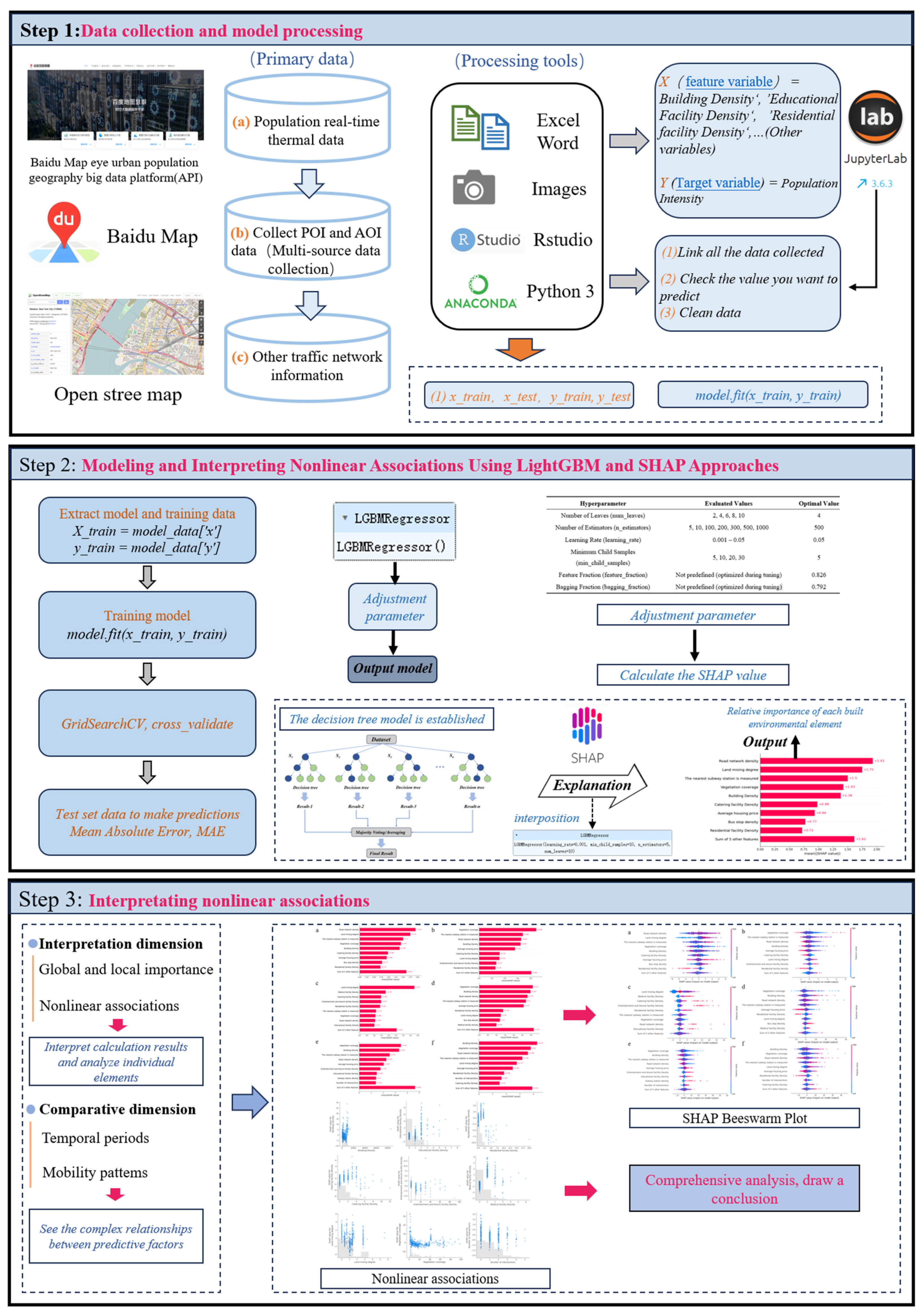
In line with the “perceptually legible 10 min EMC” paradigm, this study unfolds in three tightly linked steps (Figure 1). Step 1: Multi-source data pipeline: The target variable Y was defined as instantaneous population density (hourly active Baidu Huiyan devices per km²), representing transient human presence rather than dwell-based activity intensity. This metric captures both passage and short-term stays. To mitigate commuter bias, only weekend data were used to capture discretionary activities reflecting the intrinsic attractiveness of the built environment. Future work should integrate the Baidu Stay Points API to distinguish dwell duration (>15 min) from transient flow. Multi-source POI, AOI, traffic networks, and street-view imagery are fused to 20 street-view and GIS-based built indicators. Data cleaning, coordinate unification, and spatial linkage are executed in Python and R, and the final 4101 grids inside the empirically delimited EMC enter the modeling pool.

Step 2: Non-linear modeling and validation: Models were trained using LightGBM v3.3.5 with spatiotemporal blocked cross-validation to prevent spatial leakage: the 4101 grids were clustered into 10 contiguous spatial folds using k-means on geographic coordinates; each fold was used once for validation while the remaining nine trained the model. Early stopping was applied after 50 rounds of no improvement in validation RMSE. A random seed was fixed at 42 for reproducibility. Hyperparameters were optimized via a nested grid search. Final configuration: ‘num_leaves = 4’, ‘learning_rate = 0.05’, ‘n_estimators = 500’ (converged), ‘min_child_samples = 5’, ‘feature_fraction = 0.826’, ‘bagging_fraction = 0.792’. Training was repeated 10 times with different seeds; feature importance and SHAP values were averaged. SHapley Additive exPlanations (SHAPs) decompose marginal contributions globally and locally, revealing threshold, interaction, and saturation effects hidden from OLS or classic GWR.

Step 3: Interpretation and policy translation: Global SHAP ranking identifies the dominant drivers of vitality; SHAP dependence plots visualize non-linear response distributions for key variables. Diurnal stratification detects time-varying vulnerabilities. Scenario simulation reallocates surplus medical/dining POIs into mixed-use micro-patches under visual-quality constraints, delivering operable thresholds for “zoning–grading–quantifying”-resilient medical-circle governance.

3.3. Data Processing

In this study, a multi-source and multi-scale big data collection approach is adopted to ensure both the comprehensiveness and precision of the research. Leveraging diverse public government data resources, such as the National Geographic Information Public Service Platform’s Tianditu, the Gaode Map API, and remote sensing imagery, the study extracts crucial spatial data elements. These elements include, but are not limited to, Points of Interest (POIs), street networks, the Activity Opportunity Index (AOI), green space distribution, and river distribution. Aggregating these diverse datasets establishes a robust foundation to quantitatively analyze the impact of the built environment on regional public health (

Table 1. Multi-source spatial datasets for 10 min Emergency Medical Circle analysis, Shenzhen 2024.

Data	Data Source	Acquisition Time	Data Preprocessing and Cleaning
Road-network data	Open Street Map	2024	By processing the extracted road-network data, the topology check performed after extracting the road center line is simplified, and some actual sections are selected for comparison and proofreading.
POI	Baidu Map	2024	Select the relevant POI within a 4.5 km radius with typical medical facilities as the center, including living service facilities, entertainment facilities, healthcare facilities, public transportation stations, subway stations, etc.
Housing price	HomeLink	2024	After extracting street-housing price data (normal transaction of real estate), randomly select part of the community to view the latest transaction price.
Building profile data	Baidu Map	2024	Include the building outline (mainly for the general outline of the completed building) and combine with satellite maps and street-view images to check the data.

).

By integrating these various data sources, we can capture a more detailed and nuanced picture of the urban landscape. This comprehensive dataset facilitates the examination of multiple dimensions of the built environment, providing insights into how different elements interact and influence public health outcomes. The use of POIs and street networks facilitates the analysis of accessibility and connectivity, which are critical components of urban livability. The inclusion of the AOI offers a measure of the potential for social and economic activities within a region, reflecting the vibrancy and opportunities available to residents. Additionally, the distribution of green spaces and rivers is crucial for assessing environmental quality and its impact on physical and mental well-being.

The methodological rigor of this study is further enhanced by the spatial granularity and temporal resolution of the data, which facilitate dynamic analyses and the identification of spatial-temporal patterns. This approach not only contributes to a deeper understanding of the role the built environment plays in shaping residential spaces, but also provides valuable insights for urban planners and policy makers. By highlighting the relationships between spatial data elements and health outcomes, this research underscores the importance of integrated and data-driven planning strategies aimed at fostering healthier urban environments.

3.3.1. Recontextualizing Built-Environment Metrics for EMS Operations

To quantify the multidimensional characteristics of the 10 min Emergency Medical Circle (EMC), we established a comprehensive indicator system comprising 20 built-environment variables (

Table 2. Built-environment indicators for 10 min Emergency Medical Circle (EMC) analysis.

Dimension (Reclassified)	Research Variable (Symbol)	Calculation Description
Medical Service Centrality	Density of medical institutions (DMI)	Medical POI count/km2
Population Structure and Demand Potential	Employment–housing population balance ratio (EPR)	EPR = min(Jobs, Residents)/max(Jobs, Residents)
	Population density (PD)	Total population/grid area (persons/km2)
Physical Density and Spatial Impedance	Building density (BD)	Building footprint/grid area
Activity Intensity and Operational Friction	Density of educational facilities (DEF)	Education POI count/km2
	Density of residential facilities (DRF)	Residential POI count/km2
	Density of catering facilities (DCF)	Catering POI count/km2
	Density of recreational facilities (DRC)	Recreation POI count/km2
Open Space and Evacuation Environment	Distance to plazas and activity spaces (DPS)	DPS = mini d(p, si) where d(p, si) denotes the network distance between grid centroid p and the i-th plaza or public activity space.
	Land-use mix (LUM)	$LUM=-{\displaystyle \sum _{i=1}^k}{\displaystyle \frac{P_i\mathrm{l}\mathrm{n}{P}_i}{\ln k}}$
	Per capita green space (PGS)	Green space area/population (m2/person)
Network Permeability and Route Efficiency	Detour rate (DR)	$DR={\displaystyle \frac{1}{N}}{\displaystyle \sum _{i=1}^N}{\displaystyle \frac{S_i}{D_i}}$
	Proximity (PX)	$PX={\displaystyle \frac{1}{N}}{\displaystyle {\sum }_{i=1}^N}{d}_i$
	Number of crossing intersections (NCI)	$NCI={\displaystyle {\sum }_{i=1}^N}{I}_i$
	Road-network density (RND)	Road length/area (km/km2)
Public Transport Interaction	Subway station density (SSD)	Subway stations/km2
	Bus-stop density (BSD)	Bus stops × lines/km2
	Nearest subway station distance (NSM)	Network distance to the nearest station (m)
Environmental Experience	Air Quality Index (AQI)	Annual mean AQI value
Traffic Operating Conditions	Average daily congestion index (ACI)	Mean value of hourly congestion indices over a 24 h period

Notes: All variables are calculated at the 200 m × 200 m grid level unless otherwise specified. For the detour rate (DR), S_i denotes the shortest-path distance along the road network between an origin–destination pair, and D_i denotes the corresponding Euclidean (straight-line) distance. N represents the total number of sampled origin–destination pairs. For proximity (PX), d_i represents the network distance from the grid centroid to the i-th nearest facility, and N denotes the number of nearest facilities considered. For land-use mix (LUM), P_i denotes the proportion of land area allocated to land-use category i within a grid, and k represents the total number of land-use categories. The Air Quality Index (AQI) is obtained from the nearest national air-quality monitoring station and calculated following official standards, integrating regulated pollutants (PM_2.5, PM₁₀, SO₂, NO₂, CO, and O₃). The annual mean AQI is used in this study. The congestion index (ACI) is derived from hourly traffic condition data and averaged over a 24 h period.

). Although these indicators are widely used in urban morphology, transport accessibility, and environmental studies, their selection, reclassification, and interpretation in this research are explicitly guided by their operational relevance to emergency medical services (EMSs) rather than by conventional urban design or livability objectives.

Given the hospital-centric and strictly time-constrained nature of emergency medical response, the indicators were reorganized into a set of function-oriented dimensions that reflect the coupled mechanisms of population demand distribution, ambulance movement, and hospital service centrality within the EMC [29].

Medical service centrality serves as the structural core of the EMC. Rather than being embedded within a general service accessibility dimension, medical facility concentration is isolated to capture the gravitational role of hospitals. High levels of medical centrality not only enhance nominal service availability but also intensify localized activity concentration, potentially generating congestion, curbside interference, and access friction that directly affect ambulance approach and patient transfer [30,31,32].

Regarding the demographic logic, population structure and demand potential describe the spatial configuration of resident and daytime populations. These indicators reflect where emergency risk exposure is structurally concentrated and where latent EMS demand is likely to emerge, independent of short-term traffic conditions. By characterizing both population density and employment–housing balance, this dimension captures the underlying demographic logic shaping emergency demand within the EMC [33].

To address on-site constraints, physical density and spatial impedance focus on how the built form limits emergency operations. In dense urban environments, higher building intensity is associated with vertical evacuation challenges [34,35], reliance on elevators, limited ground-level maneuvering space, and delayed patient extraction, all of which impose operational burdens that are not reflected in horizontal travel distance alone.

At the street level, activity intensity and operational friction represent the dynamic obstacles encountered by ambulances. High concentrations of daily activities are typically associated with informal parking, delivery vehicles, pedestrian spillover, and intermittent occupation of road space [36,37,38]. These factors introduce stochastic delays that can substantially undermine effective accessibility, even in locations that appear well served in static network analyses.

Furthermore, open space and evacuation environment metrics capture the role of spatial openness. The availability and configuration of plazas, mixed-use environments, and green spaces influence both outdoor activity patterns and evacuation feasibility, thereby indirectly affecting the spatiotemporal distribution of EMS demand within the EMC.

Network permeability and route efficiency describe the structural capacity of the road system. A permeable and redundant network provides alternative routing options under congested or disrupted conditions, reducing vulnerability to localized blockages and enhancing the reliability of emergency response within strict temporal thresholds.

Public transport interaction reflects the dual role of transit infrastructure as both an accessibility enhancer and a congestion generator. High-intensity transit nodes function as population aggregation points and traffic conflict zones, shaping the operational environment through which ambulances must navigate, particularly during peak periods.

Beyond morphological attributes, environmental experience, including air quality conditions, is incorporated as a contextual moderator. Environmental quality influences residents’ willingness to engage in outdoor activities and thus indirectly reshapes population presence and latent EMS demand across time, adding a behavioral dimension to emergency accessibility assessment.

Lastly, traffic operating conditions represent the prevailing congestion environment faced by ambulances. Unlike static network indicators, this dimension directly constrains achievable response speeds, mediating the translation of spatial proximity into realized emergency access.

Taken together, this recontextualized indicator framework enables conventional built-environment metrics to be interpreted through an EMS-oriented operational lens, revealing how standard urban characteristics function differently under the time-critical conditions of emergency medical response.

3.3.2. LightGBM Modeling and SHAP Interpretation Strategy

We employed Light Gradient Boosting Machine (LightGBM) to model the non-linear 20 multi-source built-environment indicators and log-transformed hourly urban vitality. LightGBM was selected for its high computational efficiency on large-scale spatial datasets, resistance to overfitting, and seamless integration with SHAP for post hoc interpretability.

The Gradient Boosting Decision Tree (GBDT) framework builds an additive ensemble of regression trees, where each tree corrects the residuals of the preceding ensemble. The final prediction is expressed as follows:

$$f\left(x\right)=\sum _{m=1}^M{\gamma }_m{h}_m\left(x\right)$$

(1)

where $M$ is the total number of trees, $h_m\left(x\right)$ is the $m$-th weak learner (regression tree), and ${\gamma }_m$ is the optimized shrinkage weight (learning rate × tree output).

To quantify the marginal contribution of each feature and uncover non-linear threshold effects, we computed SHAP (SHapley Additive exPlanation) values. The SHAP value ${\varphi }_i$ for feature $i$ is defined as follows:

$${\varphi }_i\left(f\right)=\sum _{S\subseteq \mathcal{F}\setminus \left\{i\right\}}{\displaystyle \frac{\left|S\right|!\left(\left|\mathcal{F}\right|-\left|S\right|-1\right)!}{\left|\mathcal{F}\right|!}}\left[f\left(S\cup \left\{i\right\}\right)-f\left(S\right)\right]$$

(2)

where $\mathcal{F}$ denotes the full set of 20 predictors, $S$ is any subset of features excluding $i$, and $f(\cdot )$ is the LightGBM model’s prediction [13]. This approach ensures consistent, locally accurate, and globally interpretable feature attributions, enabling the identification of non-linear effects, interaction patterns, and threshold behaviors [11].

All analyses were conducted in Python 3.9 using LightGBM 3.3.5 for modeling, scikit-learn 1.3.2 for data preprocessing and cross-validation [24], and SHAP 0.42.1 for explainability. Hyperparameter optimization was performed via nested 10-fold cross-validation with grid search.

4. Results

4.1. Quantitative Evaluation of Residents’ Activity Characteristics in Hospital-Centered EMC

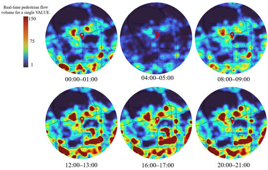
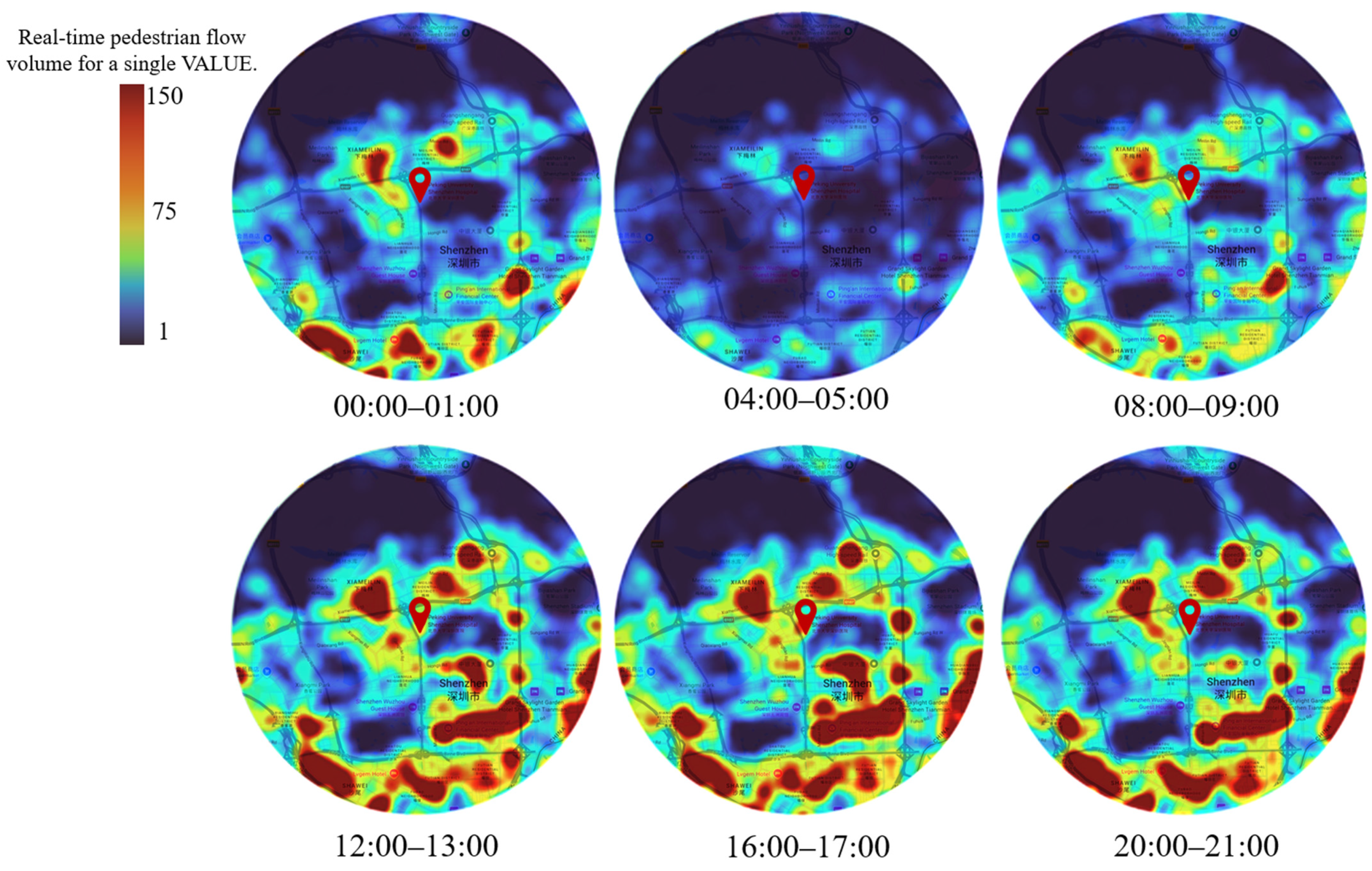
Using the Baidu Huiyan Urban Population Big Data Platform, this study quantified residents’ spatial activity intensity within 200 × 200 m grid cells (

Table 3. Sample data extraction.

Sample	City	Calculation Range (m)	Maximum Value (Day)	Minimum Value (Day)	Mean Value (Day)
1	One Avenue	200 × 200	592	3	6.932802222
2	Futian Foreign Language School	200 × 200	612	2	6.911469516
3	Shenzhen Children’s Hospital	200 × 200	529	4	14.24222328
4	Shazui Community Park	200 × 200	539	2	8.073501649

). Each heatmap value represents the number of mobile devices accessing the Baidu location SDK per hour, normalized by grid area to form an indicator of urban vitality. The dataset covers August 2024. While limiting the study to a single month introduces seasonal bias, August in Shenzhen represents a “high-stress” thermal environment, allowing us to observe how built-environment features (like greenery and shading) sustain vitality under challenging climatic conditions. Furthermore, to isolate the influence of built-environment factors, subsequent analyses used weekend data. This approach effectively isolates discretionary, lifestyle-driven behaviors from rigid weekday commuting patterns, providing a clearer reflection of the built environment’s intrinsic attractiveness rather than obligatory movement (Figure 2).

4.2. Built Environment Interactions Inside the 10 Min EMC

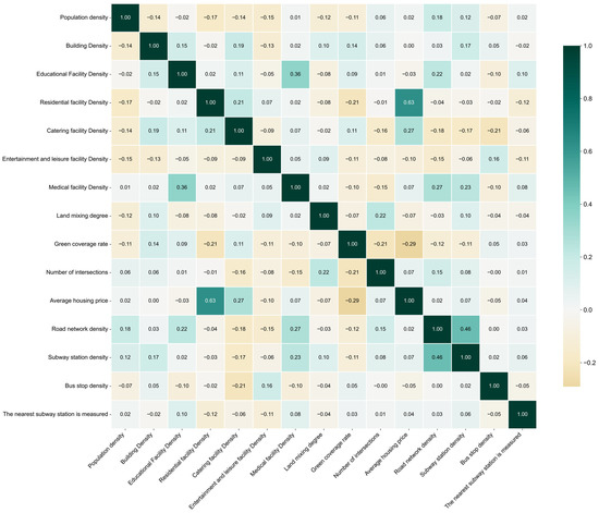
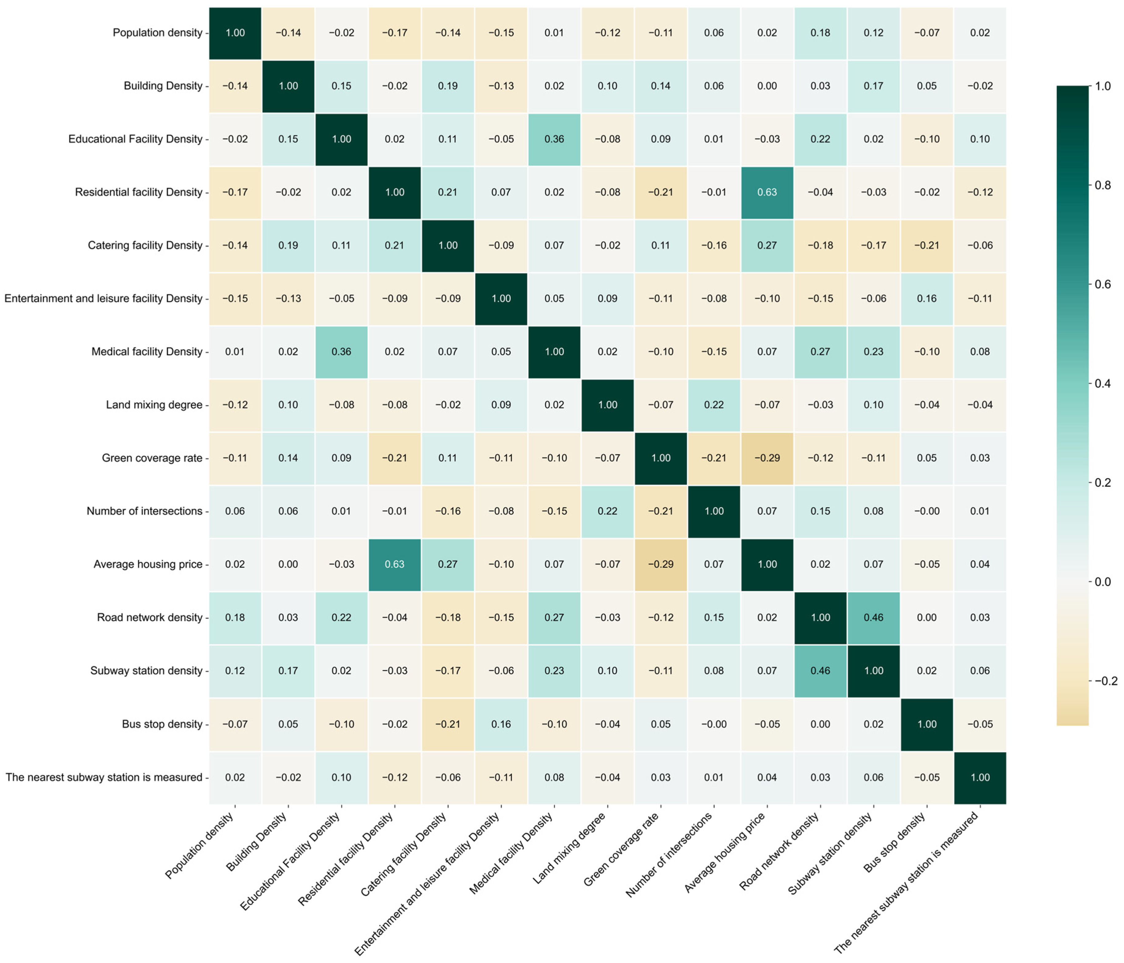
A Pearson correlation analysis of twenty built-environment variables (n = 4101 grid cells) identified four major spatial association regimes (Figure 3). (i) Density–openness trade-off: Population density showed a weak negative correlation with green coverage (r = −0.11) and a stronger inverse relation with the sky-view factor (r = −0.14, p < 0.01). (ii) Medical–POI clustering: Medical facility density correlated moderately with educational POIs (r = 0.36) and subway station density (r = 0.23), while showing a weak negative correlation with on-street green view (r = −0.10). (iii) Multimodal backbone: Road network density showed strong positive correlations with subway station density (r = 0.46) and bus-stop density (r = 0.50). Both transport indicators exhibited mild negative correlations with sky exposure (r ≈ −0.12). (iv) Collinearity diagnostics: All variables satisfied multicollinearity thresholds (r < 0.75, VIF < 3.2), confirming independence for subsequent modeling.

4.3. Hyperparameter Tuning for Gradient Boosting Decision Trees

To guard against overfitting while maximizing out-of-sample robustness, a six-dimensional grid search was executed across the GBDT hyperparameter space (

Table 4. Optimal GBDT hyperparameter configuration for the 10 min Emergency Medical Circle model.

Hyperparameter	Evaluated Values	Optimal Value
Number of Leaves (num_leaves)	2, 4, 6, 8, 10	4
Number of Estimators (n_estimators)	5, 10, 100, 200, 300, 500, 1000	500
Learning Rate (learning_rate)	0.001–0.05	0.05
Minimum Child Samples (min_child_samples)	5, 10, 20	5
Feature Fraction (feature_fraction)	Not predefined (optimized during tuning)	0.826
Bagging Fraction (bagging_fraction)	Not predefined (optimized during tuning)	0.792

). The search converged on num_leaves = 4, learning_rate = 0.05, and min_child_samples = 5, a configuration that minimized 10-fold cross-validation R² variance; larger leaf counts or lower learning rates widened the training–validation gap, signaling noise memorization. Expanding n_estimators from 5 to 1000 plateaued validation R² beyond 500 trees (ΔR² < 0.001), identifying 500 as the bias–variance efficient frontier. Stochastic subsampling stabilized at feature_fraction = 0.826 and bagging_fraction = 0.792, preserving inter-tree diversity without incurring critical information loss. These locked parameters underpin all subsequent SHAP-derived thresholds and scenario simulations, ensuring that the detected non-linearities and interaction effects are both statistically reliable and generalizable [39].

4.4. SHAP-Based Dissection of Built-Environment Determinants

To ensure the robustness of feature selection, we defined “dominant variables” using a combined stability–magnitude criterion. Specifically, the LightGBM model was executed ten independent times with distinct random seeds. A variable was classified as dominant only if it satisfied two conditions: (1) ranking within the top seven features in at least eight out of ten runs; and (2) exhibiting a mean absolute SHAP value greater than 1.0 with a standard deviation (σ) below 0.3.

Based on this criterion, seven dominant predictors—road network density, land-use entropy, building density, vegetation coverage, medical POI density, catering POI density, and distance to the nearest subway—were identified as stable core drivers of urban vitality. This parsimonious selection reflects inherent properties of the LightGBM–SHAP framework, including early variance capture by high-impact features, regularization-induced suppression of unstable or collinear splits, and diminishing marginal contributions of variables exhibiting threshold or inverted-U responses.

LightGBM sequentially reduces unexplained variance; once a variable (e.g., road network density) explains the dominant share of spatial accessibility, correlated candidates such as number of intersections or bus-stop density yield negligible marginal gains and are consequently down-weighted to near-zero SHAP contributions.

The tuned hyperparameters (feature_fraction = 0.826; min_child_samples = 5) deliberately restrict the number of candidate splits per tree, forcing the model to retain only the most stable partition rules. Variables exhibiting substantial multicollinearity (VIF > 3.2), including employment–housing balance ratio and per capita green space, are therefore filtered out during ensemble averaging.

SHAP summary plots reveal pronounced saturation or inverted-U response patterns for several excluded variables (e.g., AQI, detour rate, per capita green space), beyond which additional increments no longer alter predicted log-vitality. Their contribution variance is instead absorbed by higher-ranking proxy variables (e.g., vegetation coverage for per capita green space, land-use entropy for employment–housing balance).

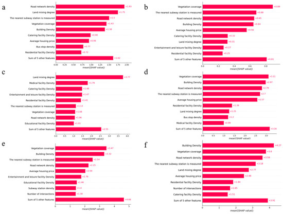
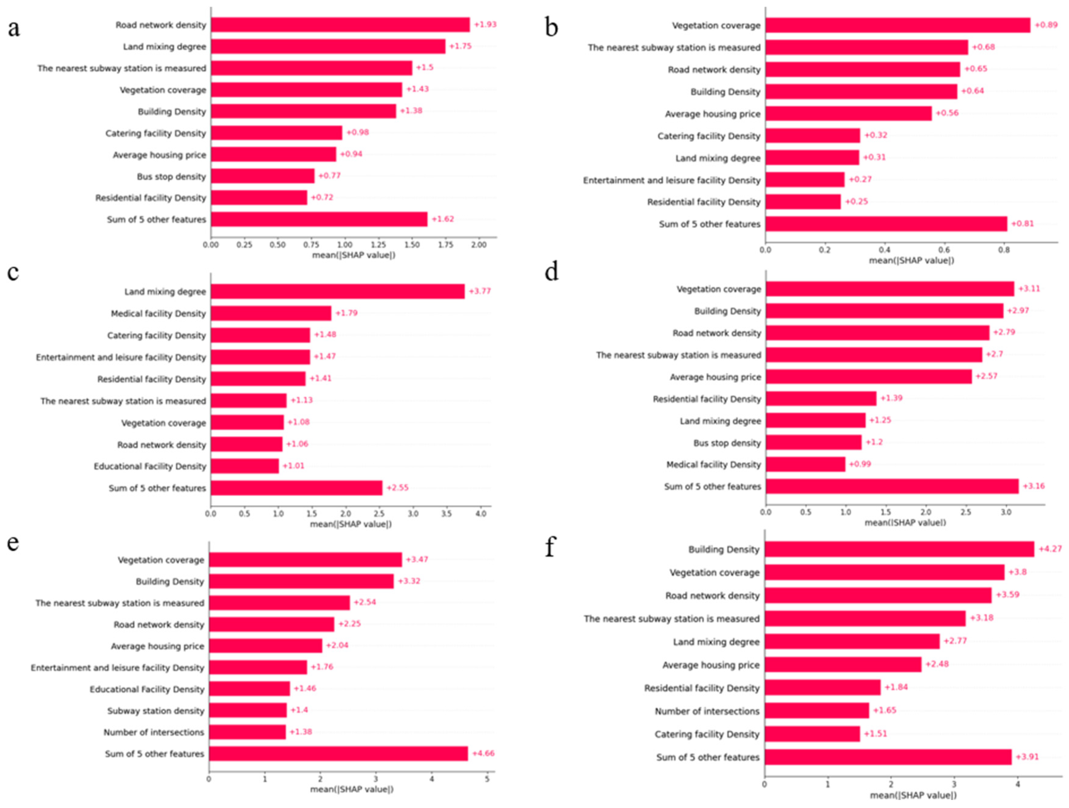
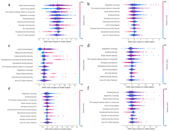
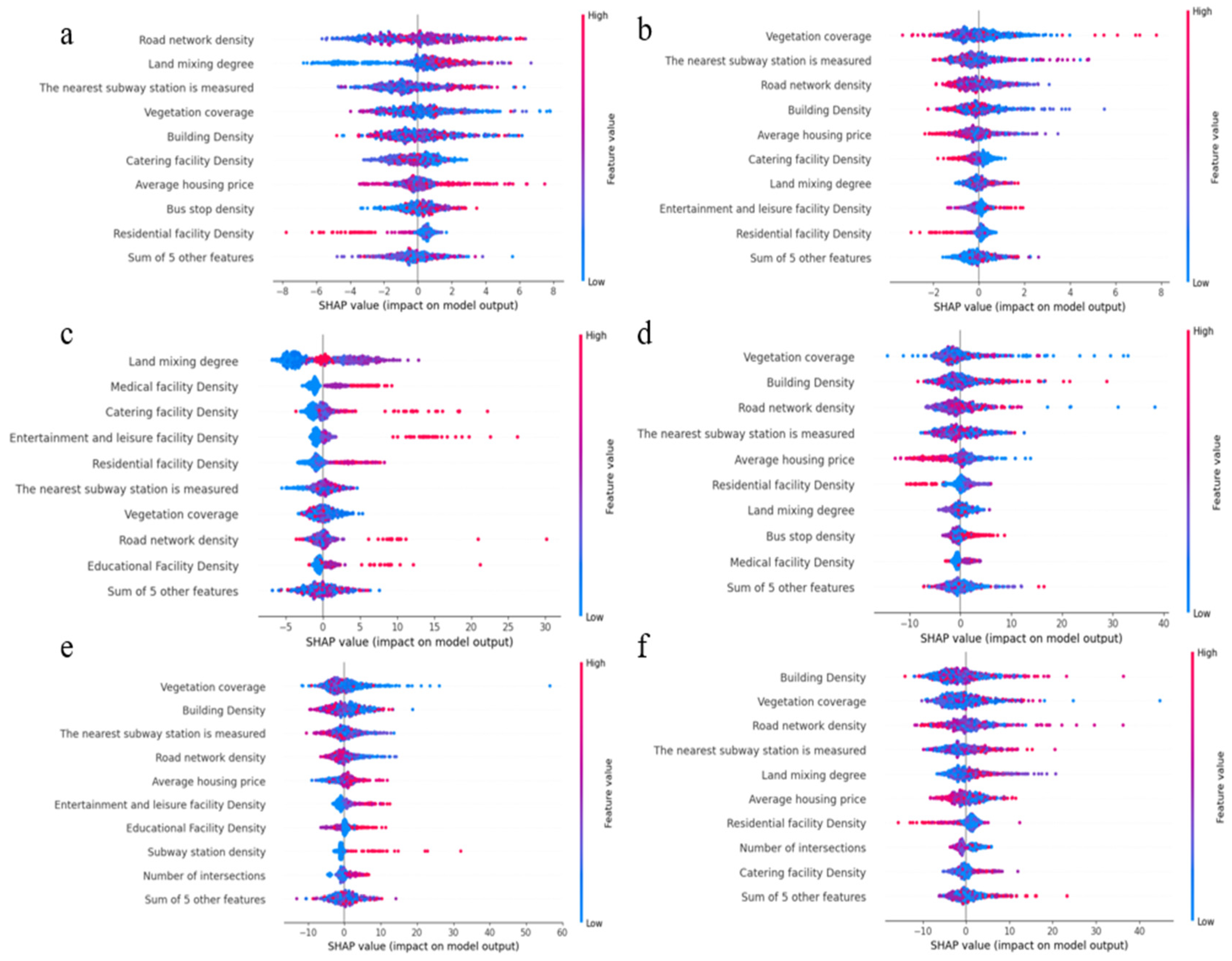
Figure 4 visualizes the global SHAP-based feature-importance ranking across different time intervals. For completeness, the plot displays the top-ranked features together with an aggregated “Sum of others” category, representing the combined contribution of all remaining indicators. However, based on the predefined stability–magnitude criterion, analytical interpretation is restricted to the seven stable dominant predictors identified above. Although other variables (e.g., average housing price) appear in the global ranking under specific temporal conditions, they do not consistently satisfy the cross-run stability requirement and are therefore treated as secondary or surrogate controls. Consequently, these seven variables constitute the dominant, non-redundant, and policy-actionable dimensions that maximize both model interpretability and planning relevance.

4.5. Mechanism Interpretation Using SHAP-Based Partial Dependence Plots

The diurnal SHAP profiles (Figure 5) show how the ranking and magnitude of dominant built-environment features change across six time intervals. During the 00:00–01:00 interval, medical facility density exhibited the highest contribution (mean |SHAP| = 2.1), serving as the primary positive predictor. Contributions from land-use entropy and vegetation coverage were negligible during this period. By 04:00–05:00, road network density became the dominant variable, with a mean |SHAP| value of +1.8, while other functional variables showed reduced influence compared to the midnight interval.

In the morning peak (08:00–09:00), land-use entropy (SHAP = +0.62) and vegetation coverage (SHAP = +0.4) showed simultaneous increases in importance, ranking as the top two drivers. During the midday period (12:00–13:00), building density and catering facility density reached their daily peak contributions (combined SHAP ≈ +5.1). Conversely, medical facility density showed negative SHAP values for grid cells with densities exceeding 2 km⁻² during this time.

Later in the afternoon (16:00–17:00), transport-related variables dominated, with distance to the nearest subway station (≤300 m, SHAP +2.5) and bus-stop density (SHAP +1.4) ranking highest. Finally, during the evening interval (20:00–21:00), entertainment and leisure facility density and land-use entropy (SHAP ≈ 0.70) emerged as the leading predictors.

4.6. Non-Linear Response Patterns in SHAP Dependence Distributions

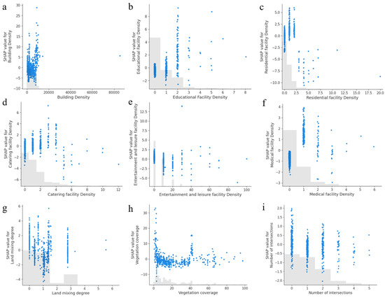
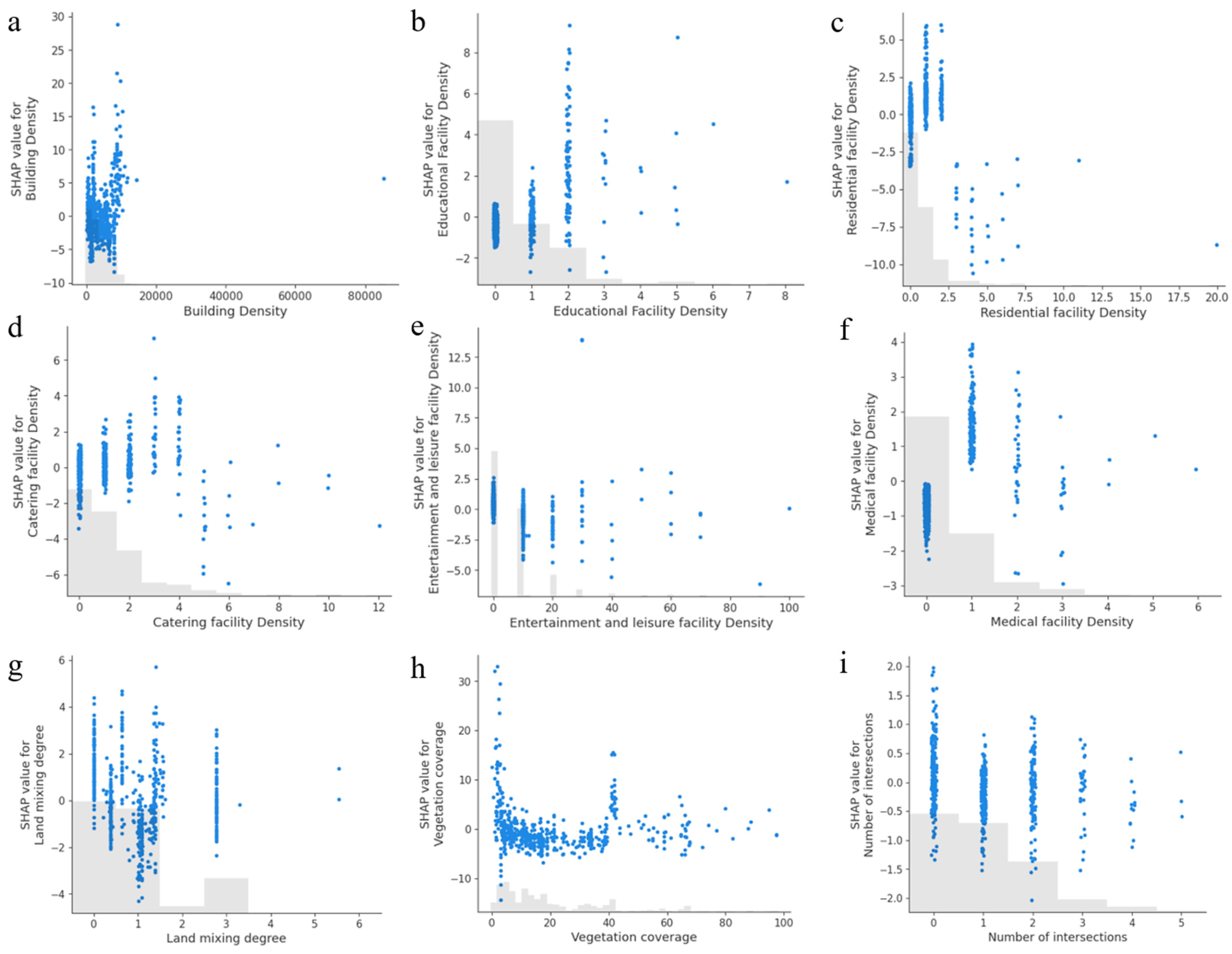
To investigate the complex, non-linear associations between built-environment features and urban vitality, we analyzed the SHAP dependence scatter plots for nine key determinants (Figure 6). Unlike linear regression coefficients, these plots visualize the distribution of marginal contributions for every individual grid cell, revealing how the impact of a feature varies across the dataset. We interpret these patterns based on the density, variance, and directional shifts in the data points, identifying functional intervals where built-environment attributes sustain or suppress vitality.

4.6.1. Physical Density and Residential Patterns

As shown in Figure 6a, in the lower-to-moderate density range (0–20,000 m²/km²), SHAP values rise steeply, confirming a robust positive correlation between physical densification and activity concentration. However, it is critical to note that the observation density drops significantly beyond 20,000 m²/km². Although the visualization indicates a potential plateauing of marginal gains in the ultra-high-density range, suggesting a saturation effect, this pattern must be interpreted with caution due to the sparsity of data points at these extremes. The apparent ‘saturation’ likely reflects the specific characteristics of the few extreme high-density outliers (e.g., CBD cores) rather than a statistically robust threshold applicable to the general urban fabric. Future studies with larger sample sizes in high-density contexts are needed to validate this boundary effect.

4.6.2. Public Service and Amenity Thresholds

Educational Facility Density (Figure 6b) displays a discrete distribution pattern where the highest concentration of positive SHAP values is confined to the range of 0–4 units km⁻². Beyond this threshold, the data points become sparse and demonstrate no further additive contribution. This distribution implies that a baseline level of educational provision is sufficient to anchor local vitality, with no evident benefit derived from excessive clustering.

Medical facility density (Figure 6f) reveals a significant polarity shift. At lower densities (0–1.5 units km⁻²), the majority of data points cluster in the positive quadrant (y > 0). However, a sharp transition occurs beyond approximately 2 units km⁻², where the center of mass of the scatter plot drops into negative values. This provides empirical evidence that while moderate medical presence supports vitality, high-density medical clusters often act as “vitality sinks” or disamenities, likely due to localized congestion or functional exclusion mechanisms.

4.6.3. Commercial and Leisure Activity Dynamics

Catering Facility Density (Figure 6d) exhibits a distribution resembling a “peak-and-decline” pattern. The density of positive SHAP values is highest between 2 and 4 units km⁻². As facility density surpasses 6 units km⁻², the scatter plot shows a downward shift, with an increasing proportion of points falling below zero. This reflects a diminishing return effect, suggesting that excessive commercial concentration may induce overcrowding or competition that dampens vitality at the grid level.

Similarly, entertainment and leisure facility density (Figure 6e) shows that positive contributions are primarily clustered at the lower end of the density spectrum (<20 units km⁻²). The sparse distribution and lack of upward momentum at higher densities suggest that entertainment venues function most effectively as dispersed anchors rather than as highly concentrated clusters within this specific EMC context.

4.6.4. Environmental Quality and Network Connectivity

Land mixing degree (Figure 6g) exhibits a robust positive cluster in the entropy range of 0.5–1.5. Grids within this interval consistently display positive SHAP values, statistically confirming that functional diversity is a stable and reliable driver of urban vitality across the study area.

Vegetation Coverage (Figure 6h) presents a complex, non-linear distribution. A dense cluster of points near 0% coverage exhibits high variance, likely corresponding to high-density urban cores where greenery is scarce but activity is high due to other factors. Notably, a secondary cluster of positive values appears around 40% coverage, indicating a potential “optimal green window” that balances ecological benefits with development intensity.

Finally, the number of intersections (Figure 6i) displays discrete vertical clusters. Grids with moderate connectivity (0–2 intersections) show a wide range of vitality outcomes, whereas the distribution tightens and remains generally positive for grids with higher connectivity. This reflects the critical role of street network permeability in facilitating movement and sustaining vitality.

4.6.5. Synthesis of Design Thresholds

Synthesizing these distributional patterns, we identify functional intervals for EMC planning. The shifts in point density and polarity—most notably the negative transition of medical facility density (>2 km⁻²) and the saturation of building density—provide quantitative reference ranges. These patterns underscore that optimal EMC vitality emerges from a balanced configuration of moderate density, functional diversity, and accessible amenities, rather than the maximization of any single metric.

5. Discussion

5.1. Summary of Key Findings

This study utilized interpretable machine learning to quantify the non-linear effects of the built environment on urban vitality within a 10 min Emergency Medical Circle (EMC). The results revealed that vitality is driven by a temporally adaptive set of dominant factors: medical facilities anchor nocturnal activity, road networks facilitate pre-dawn mobility, and mixed-use amenities drive daytime peaks [40]. Crucially, the analysis identified distinct non-linear thresholds—such as a saturation trend for building density in ultra-high intensity zones and a “disamenity threshold” for medical clustering (>2 km⁻²)—defining a specific design envelope for resilient emergency catchments.

5.2. Theoretical Implications: From Local Thresholds to Structural Tensions

The identified non-linear patterns offer theoretical insights into the mechanics of high-density urbanism. Traditional planning often assumes that increased density linearly enhances vitality. However, our findings demonstrate a density–perception decoupling, where excessive physical density reduces sky openness and visual comfort, thereby constraining vitality. This suggests that proximity to services alone is insufficient; perceptual moderators (e.g., greenery) play a critical role in sustaining human activity in compact cores.

More importantly, the observed saturation effects and “vitality sinks” (e.g., the negative impacts of medical clustering) should be situated within the broader structural dynamics of urbanization in China. Existing studies indicate that state-led development strategies have historically encouraged extreme functional concentration in cities east of the Heihe–Tengchong line to maximize economic agglomeration [41]. Our findings suggest that while this high-density development model enhances service efficiency, it simultaneously pushes urban subsystems—such as EMS catchments—toward their functional thresholds. The “tipping points” identified in Shenzhen therefore represent not merely localized traffic phenomena but spatial expressions of unresolved structural tensions embedded in the prevailing national urbanization paradigm. Under such conditions, the built environment has reached an intensity at which additional concentration no longer yields proportional benefits. Accordingly, EMCs should be understood as sensitive “pressure valves,” where the friction between policy-driven density and constrained mobility infrastructure becomes most pronounced, underscoring the need for a transition from expansion-oriented to resilience-oriented planning.

5.3. Practical Implications

To address these tensions, planning strategies for EMCs should focus on optimization rather than mere densification. First, regarding the quantitative design envelope, planners should adhere to the empirically derived ‘safe operating space’: avoiding excessive building density where marginal vitality gains diminish, maintaining land-use entropy between 0.55 and 0.70, and vegetation coverage of 35–45%. Second, to mitigate medical “island effects”—where reducing medical density is often impractical—interventions should focus on micro-renewal, such as vertical greenery and permeable boundaries, to soften the hard interfaces of large hospital campuses. Third, concerning temporal network prioritization, maintenance and traffic signal optimization should be prioritized on structural backbones to ensure 24 h resilience, recognizing that road-network density is the primary driver of pre-dawn emergency mobility.

5.4. Limitations and Future Research Directions

While this study provides a quantitative framework for analyzing vitality within the EMC, several limitations must be acknowledged to contextualize the findings.

First and foremost, the operationalization of urban vitality in this study requires careful conceptual clarification. Rather than adopting a normative or socio-cultural understanding of vitality—traditionally associated with social diversity, street-level interactions, and everyday urban life (e.g., e.g., as discussed in The Death and Life of Great American Cities)—this research employs a deliberately functional and exposure-oriented construct. Specifically, vitality is operationalized through spatiotemporal population intensity, which serves as an analytical proxy for operational pressure and risk exposure in the context of pre-hospital emergency medical services (EMSs). While this distinction reflects a conscious methodological choice aligned with EMS requirements, we explicitly acknowledge it as a limitation: areas identified as “high-vitality” zones in this analysis do not necessarily correspond to sociologically vibrant public spaces, and this quantitative proxy cannot fully capture the qualitative dimensions of urban well-being or social interaction.

Second, the reliance on Baidu Huiyan mobile positioning data introduces an inherent sampling bias. Although high-resolution, this dataset primarily captures smartphone users, potentially underrepresenting vulnerable groups such as the elderly, low-income residents, and children, who may lack digital connectivity. Since these groups are often high-frequency users of EMSs, the “vitality” proxy implies a degree of mismatch with actual demographic risk profiles. Furthermore, the current dataset records instantaneous presence but does not distinguish between transient passers-by and stationary dwellers, limiting our ability to differentiate between traffic flow and genuine activity engagement.

Third, the analysis is temporally confined to August 2024. While capturing diurnal rhythms, this single-month snapshot fails to account for seasonal variations or holiday-specific anomalies, which are critical for comprehensive year-round emergency planning. Spatially, the study focuses on Shenzhen’s highly compact urban core. The identified thresholds (e.g., the saturation of vitality benefits at high building densities) are calibrated to this ultra-high-density context. Consequently, these specific numerical values may not be directly transferable to cities with lower development intensities or polycentric layouts without local recalibration.

Fourth, regarding the modeling approach, while LightGBM effectively captures non-linearities, the SHAP interpretation framework assumes that feature contributions are largely additive. This assumption may oversimplify complex, higher-order multiplicative interactions between built-environment variables (e.g., the synergistic effect of subway proximity and commercial clustering). Additionally, the study identifies correlations and predictive associations but does not employ causal inference methods, meaning that the directionality of influence (e.g., whether amenities attract people or people attract amenities) remains statistically associative rather than causal.

To bridge these gaps, future research should prioritize three directions. Integrating transit smart-card data, census demographics, and Baidu Stay Points API data would improve the representation of diverse population groups and help distinguish dwell-based vitality from transit flow. Collaboration with EMS command centers to obtain historical ambulance GPS trajectories and actual incident data would allow a direct comparison between the predicted “latent demand” (vitality) and realized emergency events, thereby validating the proxy’s accuracy. In addition, employing causal machine learning techniques and expanding the study to multiple cities with varying densities would help disentangle causal mechanisms and establish more generalizable “resilience thresholds” applicable to global metropolitan contexts.

6. Conclusions

This study examined how the built environment shapes urban vitality within Shenzhen’s 10 min Emergency Medical Circle (EMC), revealing non-linear and temporally adaptive interactions among infrastructure, land use, and visual–perceptual elements. Key findings demonstrate that medical facilities anchor nocturnal activity, road network continuity and land-use diversity drive pre-dawn and morning mobility, and evening vitality benefits from vegetation and mixed-use integration. Counterintuitive thresholds emerged, indicating that excessive medical clustering or overly dense development can reduce vitality, while optimal levels of greenery and land-mix entropy enhance activity without causing congestion. Seven dominant factors—road network density, land-mix entropy, building density, vegetation coverage, medical and catering facility density, and proximity to subway stations—were identified as critical drivers of EMC performance. Integrating these thresholds defines a design envelope that balances emergency accessibility with sustainable urban activity.

It is important to distinguish between context-specific metrics and generalizable mechanisms. While specific quantitative thresholds (e.g., the plateauing of vitality associated with extreme building density) are calibrated to Shenzhen’s high-density context and therefore require local recalibration, the identified non-linear mechanisms demonstrate strong transferability. The inverted-U relationship associated with vegetation, the “island effect” of medical clustering, and the temporal shift in dominant drivers—from physical infrastructure at night to functional diversity during the day—reflect fundamental urban dynamics that are likely applicable to other rapidly densifying metropolitan areas. The study advances urban health and emergency planning theory by highlighting the importance of temporally sensitive, perception-informed design in resilient EMCs. Practically, the findings inform strategic distribution of facilities, mixed-use planning, and ecological moderation to optimize both emergency responsiveness and urban vitality. Overall, EMC effectiveness emerges from the dynamic interplay of functionality, spatial configuration, and perceptual experience, providing transferable insights for health-oriented urban design in global metropolitan contexts.

References

- Galderisi, A. Adapting cities for a changing climate: An integrated approach for sustainable urban development. In Proceedings of the Sustainable City IX, Siena, Italy, 23–25 September 2014; pp. 549–560. [Google Scholar]
- Jin, A.; Ge, Y.; Zhang, S. Spatial Characteristics of Multidimensional Urban Vitality and Its Impact Mechanisms by the Built Environment. Land 2024, 13, 991. [Google Scholar] [CrossRef] [Scilit]
- Laimer, P. Tourism indicators for monitoring the SDGs. In Proceedings of the Sixth UNWTO International Conference on Tourism Statistics, Measuring Sustainable Tourism, Manila, Philippines, 21–23 June 2017; pp. 1–33. [Google Scholar]
- Adedeji, O. Human Settlement and Development (EMT 506); Department of Environmental Management and Toxicology, UNAAB: Abeokuta, Nigeria, 2011. [Google Scholar]
- Panwar, A.; Olfati, M.; Pant, M.; Snasel, V. A Review on the 40 Years of Existence of Data Envelopment Analysis Models: Historic Development and Current Trends. Arch. Comput. Methods Eng. 2022, 29, 5397–5426. [Google Scholar] [CrossRef] [Scilit]
- Pourhabib Yekta, A.; Kordrostami, S.; Amirteimoori, A.; Kazemi Matin, R. Data envelopment analysis with common weights: The weight restriction approach. Math. Sci. 2018, 12, 197–203. [Google Scholar] [CrossRef] [Scilit]
- Wojcik, V.; Dyckhoff, H.; Clermont, M. Is data envelopment analysis a suitable tool for performance measurement and benchmarking in non-production contexts? Bus. Res. 2018, 12, 559–595. [Google Scholar] [CrossRef] [Scilit]
- Tavana, M.; Soltanifar, M.; Santos-Arteaga, F.J.; Sharafi, H. Analytic hierarchy process and data envelopment analysis: A match made in heaven. Expert. Syst. Appl. 2023, 223, 119902. [Google Scholar] [CrossRef] [Scilit]
- Xu, K.; Bossink, B.; Chen, Q. Efficiency Evaluation of Regional Sustainable Innovation in China: A Slack-Based Measure (SBM) Model with Undesirable Outputs. Sustainability 2019, 12, 31. [Google Scholar] [CrossRef] [Scilit]
- Yesilyurt, O.; Selamzade, F. Measuring CIS Health Systems Using the Stochastic Frontier Analysis (SFA). Econ. Reg. 2020, 16, 59–68. [Google Scholar] [CrossRef] [Scilit]
- Guo, J.; Feng, P.; Xue, H.; Xue, J. Spatial-temporal characteristics and drivers of urban built-up areas land low-carbon efficiency in China. Sci. Rep. 2025, 15, 1623. [Google Scholar] [CrossRef] [Scilit] [PubMed]
- Liu, P.; Luo, Z. A Measurement and Analysis of the Growth of Urban Green Total Factor Productivity——Based on the Perspective of Energy and Land Elements. Front. Environ. Sci. 2022, 10, 838748. [Google Scholar] [CrossRef] [Scilit]
- Zhang, Z.; Xiao, R.; Yu, W.; Liu, Y.; Lin, M.; Wang, M. Characterizing Factors Associated with Built-Up Land Expansion in Urban and Non-Urban Areas from a Morphological Perspective. Sustainability 2017, 9, 1411. [Google Scholar] [CrossRef] [Scilit]
- Nick, G.A.; Savoia, E.; Elqura, L.; Crowther, M.S.; Cohen, B.; Leary, M.; Wright, T.; Auerbach, J.; Koh, H.K. Emergency preparedness for vulnerable populations: People with special health-care needs. Public Health Rep. 2009, 124, 338. [Google Scholar] [CrossRef] [Scilit] [PubMed]
- Kailes, J.I.; Enders, A. Moving beyond “special needs” A function-based framework for emergency management and planning. J. Disabil. Policy Stud. 2007, 17, 230–237. [Google Scholar] [CrossRef] [Scilit]
- Rusca, M.; Messori, G.; Di Baldassarre, G. Scenarios of human responses to unprecedented social-environmental extreme events. Earth’s Future 2021, 9, e2020EF001911. [Google Scholar] [CrossRef] [Scilit]
- VanWey, L.K.; Ostrom, E.; Meretsky, V. Theories underlying the study of human-environment interactions. In Seeing the Forest and the Trees: Human-Environment Interactions in Forest Ecosystems; The MIT Press: Cambridge, MA, USA, 2005; pp. 23–56. [Google Scholar]
- Sahil; Sood, S.K. Fog-Cloud centric IoT-based cyber physical framework for panic oriented disaster evacuation in smart cities. Earth Sci. Inform. 2022, 15, 1449–1470. [Google Scholar] [CrossRef] [Scilit]
- Mrema, G.C.; Gumbe, L.O.; Chepete, H.J.; Agullo, J.O. Rural Structures in the Tropics: Design and Development; Food and Agriculture Organization of the United Nations: Rome, Italy, 2012. [Google Scholar]
- Lenton, T.M.; Milkoreit, M.; Willcock, S.; Abrams, J.F.; Mc Kay, D.L.A.; Buxton, J.E.; Donges, J.; Loriani, S.; Wunderling, N.; Alkemade, F. Global Tipping Points Report 2025; University of Exeter: Exeter, UK, 2025. [Google Scholar]
- Tao, Z.; Zhao, M. Planning for equal transit-based accessibility of healthcare facilities: A case study of Shenzhen, China. Socio-Econ. Plan. Sci. 2023, 88, 101666. [Google Scholar] [CrossRef] [Scilit]
- Pinter-Wollman, N.; Jelic, A.; Wells, N.M. The impact of the built environment on health behaviours and disease transmission in social systems. Philos. Trans. R. Soc. Lond. B Biol. Sci. 2018, 373, 20170245. [Google Scholar] [CrossRef] [Scilit]
- Melis, G.; Gelormino, E.; Marra, G.; Ferracin, E.; Costa, G. The Effects of the Urban Built Environment on Mental Health: A Cohort Study in a Large Northern Italian City. Int. J. Environ. Res. Public Health 2015, 12, 14898–14915. [Google Scholar] [CrossRef] [Scilit]
- Zhang, Y.; Tzortzopoulos, P.; Kagioglou, M. Healing built-environment effects on health outcomes: Environment–occupant–health framework. Build. Res. Inf. 2018, 47, 747–766. [Google Scholar] [CrossRef] [Scilit]
- Du, M.; Cheng, L.; Li, X.; Yang, J. Factors affecting the travel mode choice of the urban elderly in healthcare activity: Comparison between core area and suburban area. Sustain. Cities Soc. 2020, 52, 101868. [Google Scholar] [CrossRef] [Scilit]
- Koohsari, M.J.; Mavoa, S.; Villanueva, K.; Sugiyama, T.; Badland, H.; Kaczynski, A.T.; Owen, N.; Giles-Corti, B. Public open space, physical activity, urban design and public health: Concepts, methods and research agenda. Health Place 2015, 33, 75–82. [Google Scholar] [CrossRef] [Scilit] [PubMed]
- Li, C.; Yu, L.; Oloo, F.; Chimimba, E.G.; Kambombe, O.; Asamoah, M.; Opoku, P.D.; Ogweno, V.W.; Fawcett, D.; Hong, J. Slum and urban deprivation in compacted and peri-urban neighborhoods in sub-Saharan Africa. Sustain. Cities Soc. 2023, 99, 104863. [Google Scholar] [CrossRef] [Scilit]
- Chao, R.; Xue, D.; Wang, B. Evaluating Human Needs: A Study on the Spatial Justice of Medical Facility Services in Social Housing Communities in Guangzhou. Land 2024, 13, 1109. [Google Scholar] [CrossRef] [Scilit]
- Purdy, E.I.; McLean, D.; Alexander, C.; Scott, M.; Donohue, A.; Campbell, D.; Wullschleger, M.; Berkowitz, G.; Winearls, J.; Henry, D. Doing our work better, together: A relationship-based approach to defining the quality improvement agenda in trauma care. BMJ Open Qual. 2020, 9, e000749. [Google Scholar] [CrossRef] [Scilit] [PubMed]
- Carter, J.G.; Cavan, G.; Connelly, A.; Guy, S.; Handley, J.; Kazmierczak, A. Climate change and the city: Building capacity for urban adaptation. Prog. Plan. 2015, 95, 1–66. [Google Scholar] [CrossRef] [Scilit]
- Liu, W.; Zheng, S.; Hu, X.; Wu, Z.; Chen, S.; Huang, Z.; Zhang, W. Effects of spatial scale on the built environments of community life circles providing health functions and services. Build. Environ. 2022, 223, 109492. [Google Scholar] [CrossRef] [Scilit]
- Dhar, T.K.; Khirfan, L. A multi-scale and multi-dimensional framework for enhancing the resilience of urban form to climate change. Urban Clim. 2017, 19, 72–91. [Google Scholar] [CrossRef] [Scilit]
- Hsu, K.-W.; Chao, J.-C. Study on the Value Model of Urban Green Infrastructure Development—A Case Study of the Central District of Taichung City. Sustainability 2021, 13, 7402. [Google Scholar] [CrossRef] [Scilit]
- Kopyt, M.; Piotrowski, P.; Baczyński, D. Short-Term Energy Generation Forecasts at a Wind Farm—A Multi-Variant Comparison of the Effectiveness and Performance of Various Gradient-Boosted Decision Tree Models. Energies 2024, 17, 6194. [Google Scholar] [CrossRef] [Scilit]
- Hancock, J.T.; Khoshgoftaar, T.M. CatBoost for big data: An interdisciplinary review. J. Big Data 2020, 7, 94. [Google Scholar] [CrossRef] [Scilit]
- Wu, J.; Li, C. Illustrating the nonlinear effects of urban form factors on transportation carbon emissions based on gradient boosting decision trees. Sci. Total Environ. 2024, 929, 172547. [Google Scholar] [CrossRef] [Scilit]
- Li, Q.; Wang, Y.; Shao, Y.; Li, L.; Hao, H. A comparative study on the most effective machine learning model for blast loading prediction: From GBDT to Transformer. Eng. Struct. 2023, 276, 115310. [Google Scholar] [CrossRef] [Scilit]
- Yang, L.; Yu, B.; Liang, Y.; Lu, Y.; Li, W. Time-varying and non-linear associations between metro ridership and the built environment. Tunn. Undergr. Space Technol. 2023, 132, 104931. [Google Scholar] [CrossRef] [Scilit]
- Kushwah, J.S.; Kumar, A.; Patel, S.; Soni, R.; Gawande, A.; Gupta, S. Comparative study of regressor and classifier with decision tree using modern tools. Mater. Today Proc. 2022, 56, 3571–3576. [Google Scholar] [CrossRef] [Scilit]
- Rokach, L. Decision forest: Twenty years of research. Inf. Fusion 2016, 27, 111–125. [Google Scholar] [CrossRef] [Scilit]
- Morán Uriel, J.; Camerin, F.; Córdoba Hernández, R. Urban horizons in China: Challenges and opportunities for community intervention in a country marked by the heihe-tengchong line. In Diversity as Catalyst: Economic Growth and Urban Resilience in Global Cityscapes; Springer: Berlin/Heidelberg, Germany, 2024; pp. 105–125. [Google Scholar]
Disclaimer/Publisher’s Note: The statements, opinions and data contained in all publications are solely those of the individual author(s) and contributor(s) and not of MDPI and/or the editor(s). MDPI and/or the editor(s) disclaim responsibility for any injury to people or property resulting from any ideas, methods, instructions or products referred to in the content. |
© 2026 by the authors. Licensee MDPI, Basel, Switzerland. This article is an open access article distributed under the terms and conditions of the Creative Commons Attribution (CC BY) license.