A Nonlinear SW Model for Laterally Loaded Piles in the Proximity of Sandy Slopes with Consideration of Slope Surface Deformation

Abstract

This paper develops a nonlinear strain wedge (SW) model for analyzing laterally loaded piles installed in the proximity of sandy slopes, with consideration of slope surface deformation. This model is first developed for piles at the slope crest, characterizing the slope surface deformation to calculate soil strain and incorporating the reduction in effective vertical stress. Furthermore, this model provides a smooth transition between piles located at varying distances from the slope and those at the crest, accounting for varying near-slope distances. Thus, a comprehensive model is established that considers the influence of slope effects on pile–soil interactions. Predictions from the proposed model show good agreement with a series of centrifuge tests and three model tests. Finally, the effects of applied load, slope angle, near-slope distance, Poisson’s ratio, and friction angle on the pile response, slope surface deformation, and soil deformation are discussed.

1. Introduction

Piles are widely employed in engineering structures to withstand lateral loads and are inevitably constructed in the proximity of slopes. Examples include onshore piles for bridges and transmission towers in mountainous areas or along the valleys, as well as offshore piles for wind turbines and docks along coastal slopes. These slope effects considerably diminish the lateral capacity of the piles, thereby posing an increased risk to the safety of the superstructure.

To evaluate the slope effects, research has primarily focused on the reduction in lateral soil resistance. Several pile tests [1,2,3] were carried out and some reduction factors for the p-y curve model have been proposed. Considering the reduction in the passive wedge, the ultimate soil resistance was evaluated by the failure wedge model [4,5,6,7]. Both the ultimate soil resistance and the initial stiffness were modified by numerical inversions [8,9,10,11,12]. However, these approaches are dependent on empirical test data or numerical simulations.

The SW model proposed by Norris [13] and Ashour et al. [14] established a relationship between three-dimensional pile–soil interaction and a one-dimensional Winkler beam, providing an approach that does not require test data. However, its fundamental assumption of uniform soil strain does not accurately represent practical conditions. Yang et al. [15] proposed a nonlinear SW model, which calculates non-uniform soil strain along the depth by explicitly considering the deformed compatibility between the pile and soil. To incorporate the slope effect, Peng et al. [16] and Hemel et al. [17] extended the SW model by accounting for modifications in effective vertical stress and wedge geometry, developing models applicable to piles installed near slopes. Yet, a critical aspect remains unaddressed. That is, the slope surface itself experiences outward displacement [18]. Although Jiang et al. [19] have incorporated slope surface deformation into an SW model, the model retained the uniform-strain assumption. Therefore, it is urgent to develop a nonlinear SW model that takes into account slope surface deformation.

This study develops a nonlinear SW model for laterally loaded piles in the proximity to sandy slopes incorporating slope effects, including slope surface deformation and reduction in effective vertical stress. The model is validated against a series of centrifuge tests. Furthermore, the influence of applied load, slope angle, near-slope distance, Poisson’s ratio, and friction angle on the response of pile and soil is investigated.

2. Nonlinear SW Model for Laterally Loaded Piles in Level Ground

The lateral pile–soil interaction for a square pile with an embedded length L and side length D, installed in level ground and subjected to a lateral load H at a height e above the mudline, can be analyzed using the SW model. This model determines the subgrade reaction modulus ($k$), which is required for solving the governing differential equation.

$$EI{\displaystyle \frac{d{y}^4}{d{z}^4}}+ky=0$$

(1)

where $EI$ is the flexural stiffness of the pile, and $y$ is the lateral pile displacement at depth $z$.

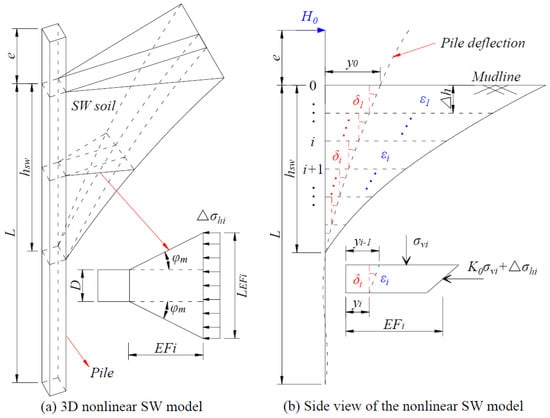
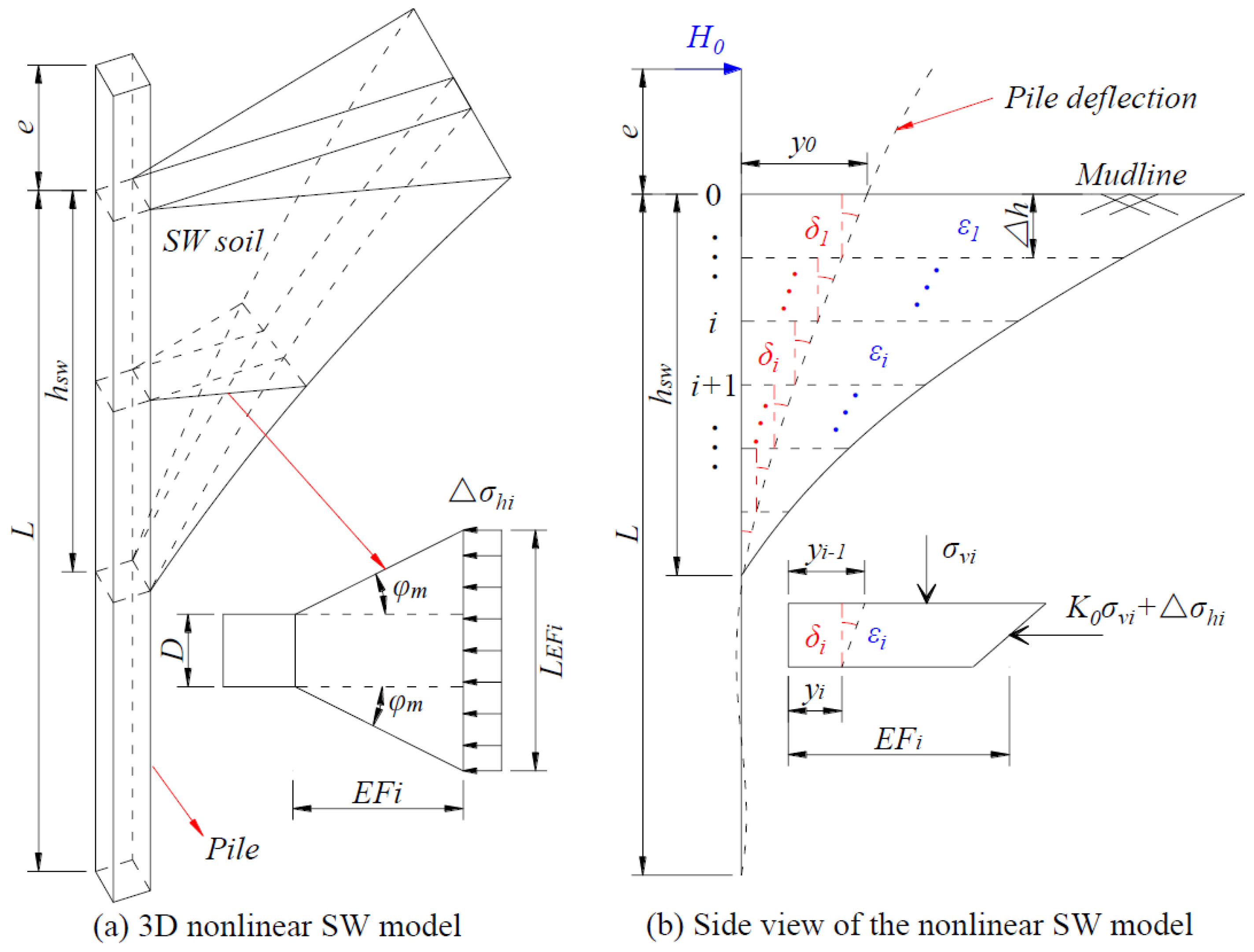
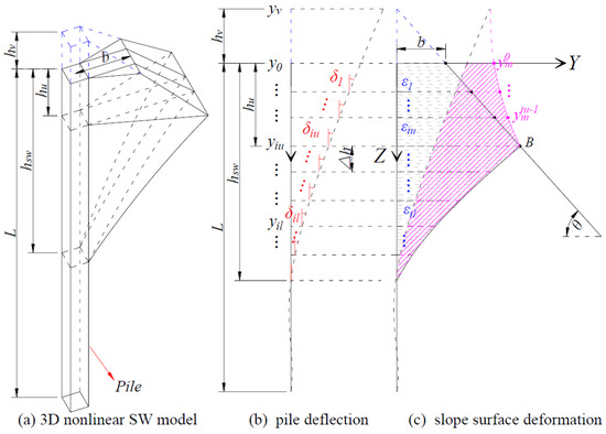
The original SW model [13,14] idealizes the soil in the passive compression zone ahead of the pile as a tetrahedral wedge. A fundamental assumption of this model is uniform soil strain within the idealized wedge, which may not accurately represent practical conditions, where soil strain often exhibits spatial variation. To address this limitation, Yang et al. [15] developed a nonlinear SW model. This nonlinear model calculates a non-uniform strain distribution along the depth by explicitly considering the deformed compatibility between the pile and soil; that is, the lateral pile displacement at any depth must equal the cumulative lateral deformation of the adjacent soil wedge (Figure 1).

Figure 1. Nonlinear SW model in level ground.

3. Nonlinear SW Model for Laterally Loaded Piles in the Proximity to Slopes

3.1. Nonlinear SW Model for Laterally Loaded Piles at the Slope Crest

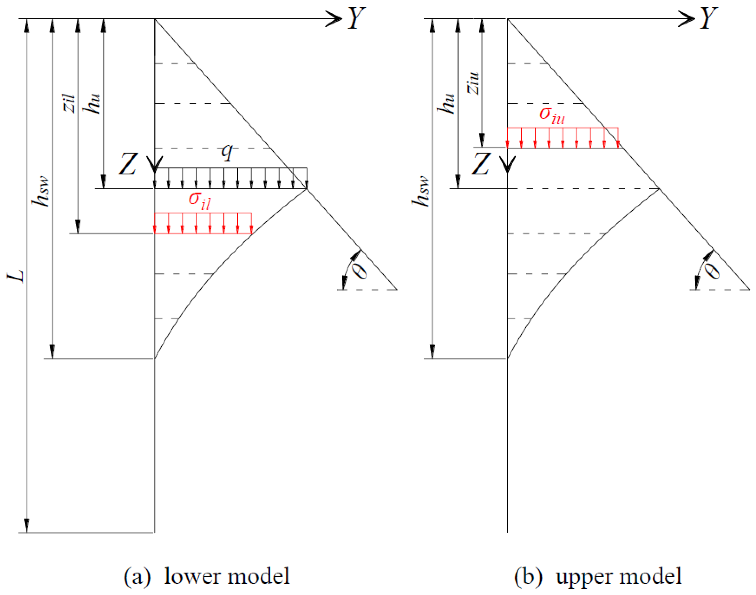
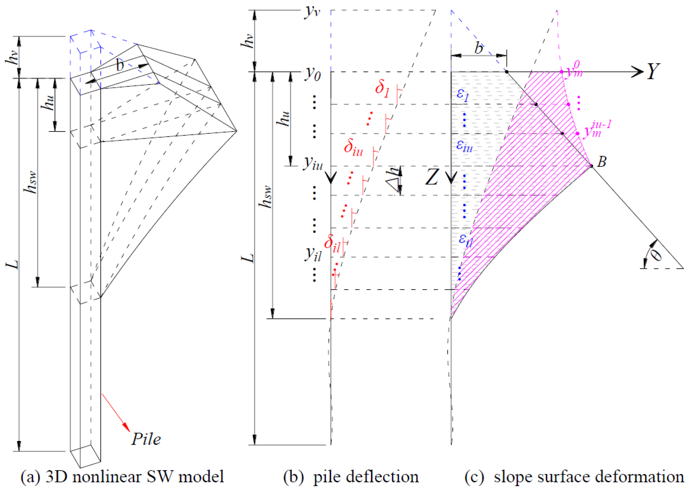
For a laterally loaded pile installed at the crest of a slope, where its near-slope distance (b) is 0.5D, a passive compression zone develops toward the slope surface. Due to the presence of this boundary, the SW model is conceptually divided into two segments: an upper model ($z\le h_u$) and a lower model ($h_u<z\le h_{sw}$), as depicted in Figure 2. The depth of $h_u$ marks the boundary between the upper and lower models and is related to the geometry of the slope and the passive compression zone. A key feature of the upper model is the absence of confining soil beyond the passive zone; consequently, the slope surface itself experiences outward displacement, as reported by Liu and Jiang [20,21]. As reported by Qian et al. [18], the distribution of the slope surface displacement is complex, decreasing with depth and varying perpendicular to the loading direction. For simplicity, this is idealized as a plane problem. Based on the above characteristic, the nonlinear SW model incorporates the following modifications:

(1)

At the mudline (z = 0), the soil adheres to the pile and moves synchronously with it; therefore, the pile displacement equals that of the slope surface. At the interface between the upper and lower models, the displacement of the slope surface is zero. The deformed shape of the slope surface after loading is assumed to follow a circular arc [19]. This arc is tangent to the original slope surface, with the tangent point located on the slope at a depth of $h_u$.

(2)

In the lower model, the deformation compatibility between pile and soil remains consistent with that in level ground. For the upper model, the lateral pile displacement at any depth must satisfy deformation compatibility, equaling the sum of the cumulative lateral deformation of the adjacent soil wedge and the displacement of the slope surface.

(3)

The reduction in the volume of the upper model leads to varying degrees of reduction in the effective vertical stress acting on both the upper and lower sections of the model.

Figure 2. Nonlinear SW model at slope crest.

Figure 2. Nonlinear SW model at slope crest.

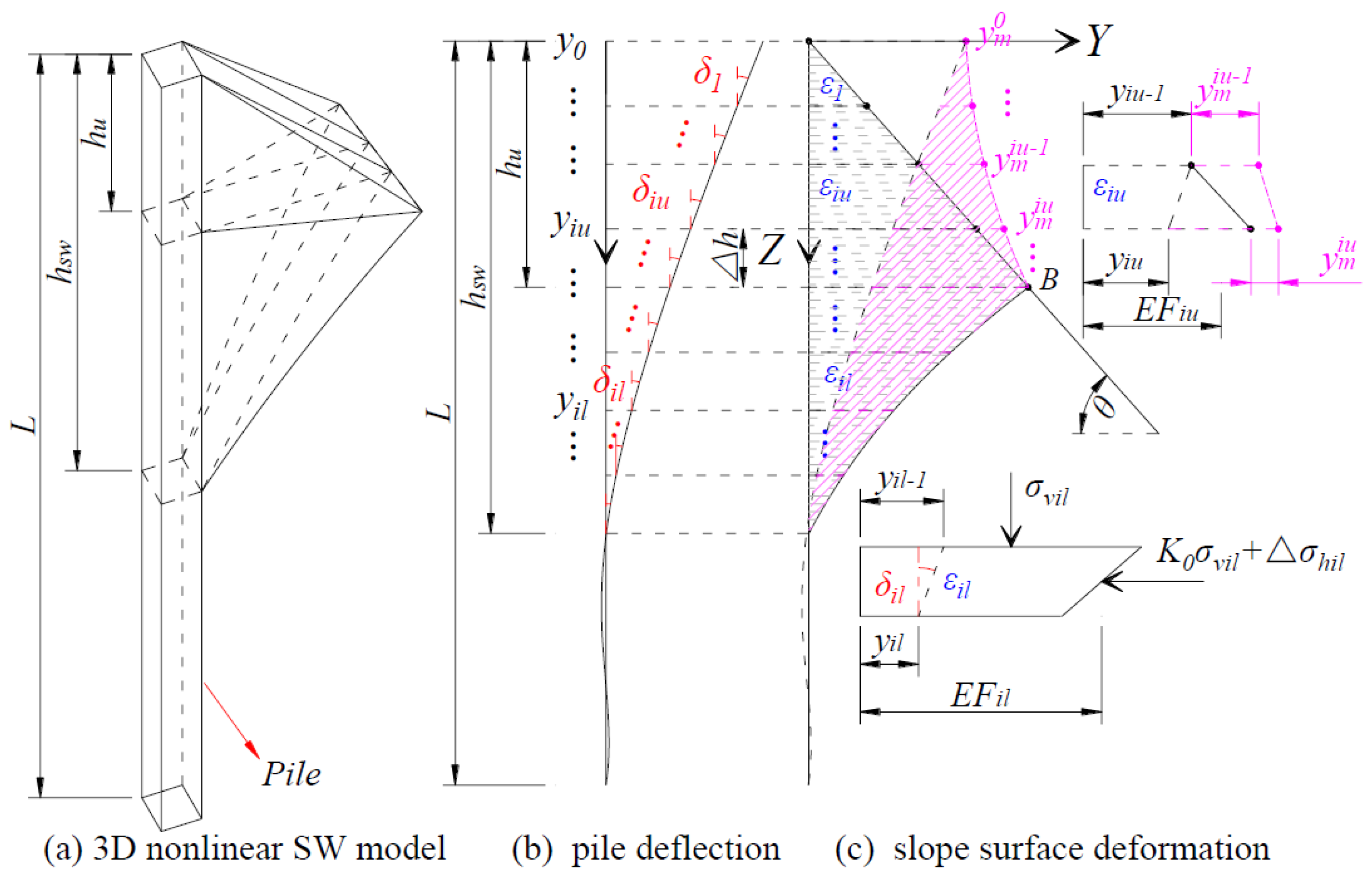
Based on the above modifications, a nonlinear SW model applicable to piles at the crest of a slope is developed. In this model, key parameters, the fan angle (${\phi }_m$), the width of the pile to the front wedge surface ($\overline{{EF}_i}$), the depths of the upper model ($h_u$) and the whole model ($h_{sw}$), and the soil strain ($\mathsf{\epsilon }$), evolve with variations in slope geometry, soil parameters, pile properties, and load levels. Consequently, the slope surface deformation also varies with these factors.

(1)

Lower Model

The SW model is discretized into N layers, each with a thickness of $∆h$. The analysis of the lower model follows the method proposed by Yang et al. [15], which further accounts for the reduction in effective vertical stress.

The pile deflections at the upper and lower nodes of a given layer il are denoted as $y_{il-1}$ and $y_{il}$, respectively (Figure 2b). In accordance with the deformation compatibility between the pile and soil, these deflection values are directly equated to the soil compressions at the corresponding nodes (Figure 2c). The deflection pattern (${\delta }_{il}$) is therefore calculated as:

$$\mathrm{t}\mathrm{a}\mathrm{n}{\delta }_{il}={\displaystyle \frac{y_{il-1}-y_{il}}{∆h}}$$

(2)

The soil strain (${\epsilon }_{il}$) is determined from the average soil compression and the lateral width of the SW model ($\overline{{EF}_{il}}$), as defined by Equation (3).

$${\epsilon }_i={\displaystyle \frac{y_{il-1}+y_{il}}{2\overline{{EF}_{il}}}}$$

(3)

The relationship between the deflection pattern (${\delta }_{il}$), soil strain (${\epsilon }_{il}$), and mobilized friction angle (${\phi }_{mil}$) is expressed by Equation (4) [14].

$${\delta }_{il}={\displaystyle \frac{(1+\nu ){\epsilon }_{il}}{2}}cos{\phi }_{mil}$$

(4)

where $\nu$ is the Poisson’s ratio of sand.

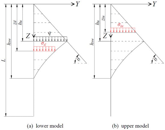
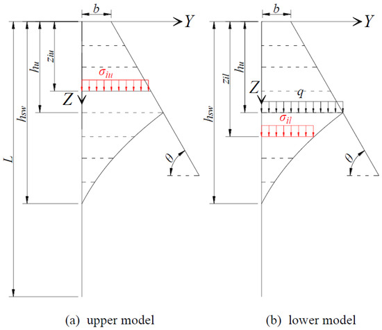
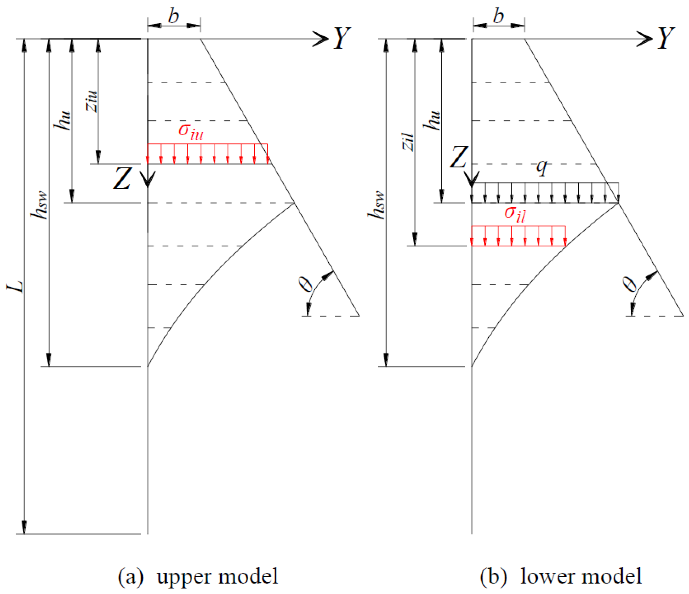
The effect of the upper model is simulated as a uniformly distributed load applied to the top of the lower model (Figure 3a). Consequently, the effective vertical stress (${\sigma }_{3il}$) at depth $z_{il}$ is:

$${\sigma }_{3il}=\gamma {(z}_{il}-{\displaystyle \frac{h_u}{2}})$$

(5)

Figure 3. Effective vertical stress at slope crest along the depth.

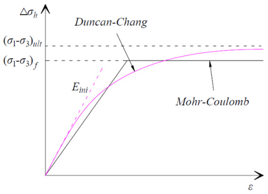
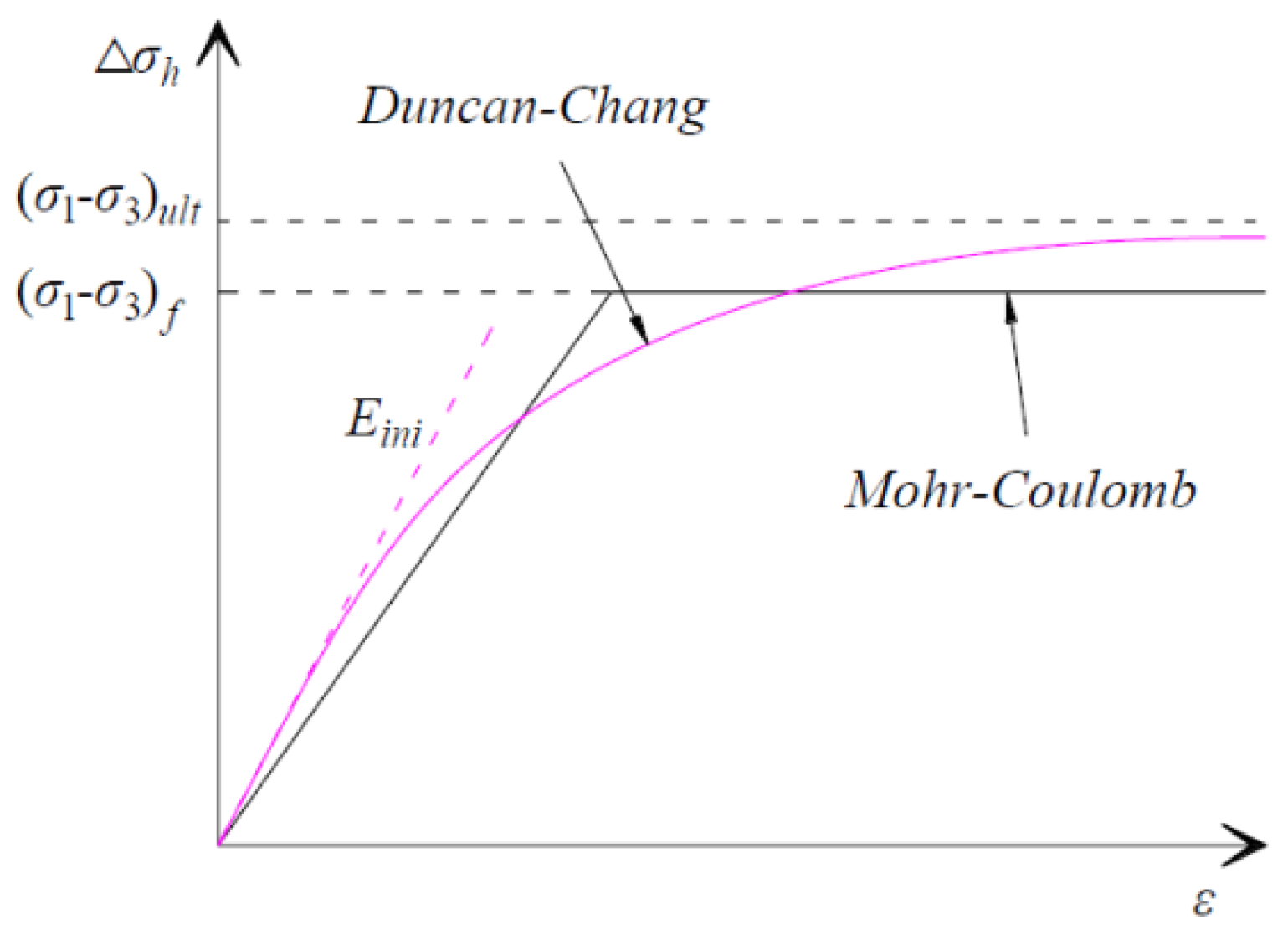
As illustrated in Figure 4, the following hyperbolic soil stress–strain relationship [22] is applied to calculate the horizontal stress change (${∆\sigma }_{hil}$).

$${∆\sigma }_{hil}={\sigma }_{1il}-{\sigma }_{3il}={\displaystyle \frac{{\epsilon }_{il}}{\frac{1}{E_{il}}+\frac{{\epsilon }_{il}}{{{(\sigma }_{1il}-{\sigma }_{3il})}_{ult}}}}$$

(6)

where $E_{il}$ and ${{(\sigma }_{1il}-{\sigma }_{3il})}_{ult}$ denote the initial stiffness and the ultimate value of the stress–strain relationship, respectively. These values are calculated as follows:

$$E_{il}=K_E{P}_a{\left({\displaystyle \frac{{\sigma }_{3il}}{P_a}}\right)}^n$$

(7)

$${{(\sigma }_{1il}-{\sigma }_{3il})}_{ult}={\displaystyle \frac{{({\sigma }_{1il}-{\sigma }_{3il})}_f}{R_f}}$$

(8)

$${({\sigma }_{1il}-{\sigma }_{3il})}_f={∆\sigma }_{hfil}={\sigma }_{3il}\left[{tan}^2\left(45°+{\displaystyle \frac{\phi }{2}}\right)-1\right]$$

(9)

where $K_E$ is the stiffness number, $n$ is stiffness exponent, and $R_f$ is the failure ratio. The values of $K_E$, $R_f$, and $n$ are related to relative density ($D_r$), with their values summarized in Table 1 based on the research by Byrne et al. [23]. $P_a = 1$00 $\mathrm{k}\mathrm{P}\mathrm{a}$ represents the atmospheric pressure.

Figure 4. Hyperbolic soil stress–strain relationship.

Table 1. Parameters of Duncan–Chang model.

${\mathit{D}}_{\mathit{r}}$ (%)	${\mathit{K}}_{\mathit{E}}$	$\mathit{n}$	${\mathit{R}}_{\mathit{f}}$
25	250–500	0.5	0.9
50	450–900	0.5	0.8
75	850–1500	0.5	0.7
100	1500–3000	0.5	0.6

The relationship between the mobilized friction angle (${\phi }_{mi}$) and the horizontal stress change (${∆\sigma }_{hil}$) is given by Equation (10) [14].

$${SL}_{il}={\displaystyle \frac{{∆\sigma }_{hil}}{{∆\sigma }_{hfil}}}={\displaystyle \frac{{tan}^2\left(45°+\frac{{\phi }_{mil}}{2}\right)-1}{{tan}^2\left(45°+\frac{\phi }{2}\right)-1}}$$

(10)

where ${SL}_i$ is the stress level, and its value is limited to 1.

(2)

Upper Model

As shown in Figure 2c, the circular arc representing the deformed slope surface passes through two fixed points: the point at the mudline with coordinates ($y_0,0$), and the point at the interface between the upper and lower models with coordinates ($h_u/tan\theta , h_u$). The geometry of this arc is governed by the following equations:

$${R_s}^2=\{\begin{array}{c}{(y_s-y_0)}^2+{(z_s)}^2\\ {(y_s-{\displaystyle \frac{h_u}{tan\theta }})}^2+{(z_s-h_u)}^2\end{array}$$

(11)

$$z_s=-{\displaystyle \frac{1}{\mathit{tan}\left(\theta \right)}}\left(y_s-{\displaystyle \frac{h_u}{tan\theta }}\right)+h_u$$

(12)

$${(\overline{{EF}_{iu}}+y_{im}-y_s)}^2+{(z_{iu}-z_s)}^2={R_s}^2$$

(13)

$$\overline{{EF}_{iu}}={\displaystyle \frac{z_{iu}}{tan\theta }}$$

(14)

where ($y_s$, $z_s$) are the coordinates of the center of the circular arc, $R_s$ is its radius, and $y_{im}$ denotes the displacement of the slope surface at depth $z_{iu}$.

For a given layer iu within the upper model, the pile deflections at its upper and lower nodes are denoted as $y_{iu-1}$ and $y_{iu}$, the corresponding slope surface displacements are $y_{im-1}$ and $y_{im}$, and the soil strain in the layer is ${\epsilon }_{iu}$. According to the deformation compatibility, the following expression is obtained.

$${\displaystyle \frac{{y_{iu-1}+y}_{iu}}{2}}={\displaystyle \frac{y_{im-1}+y_{im}}{2}}+{\epsilon }_{iu}{\displaystyle \frac{z_{iu-1}+z_{iu}}{2tan\theta }}$$

(15)

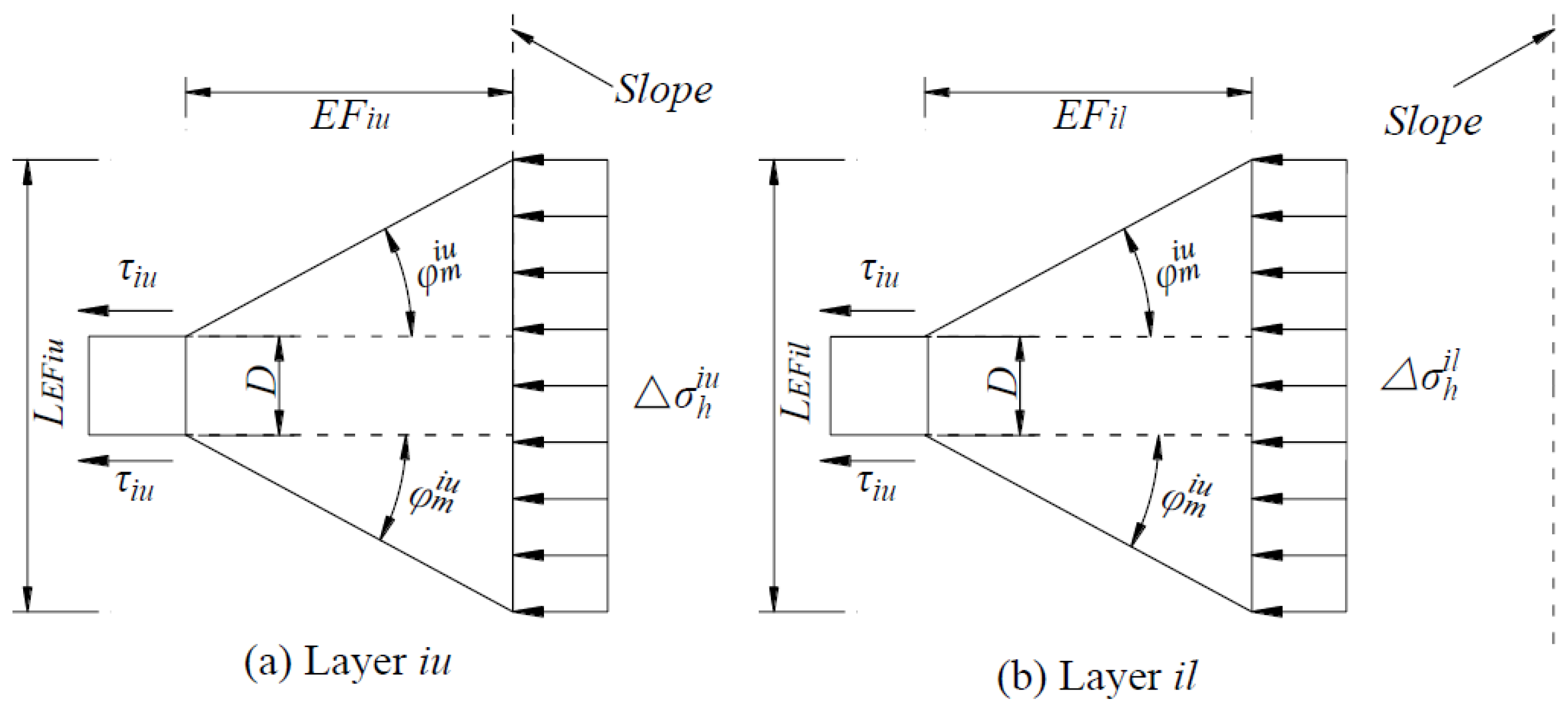
The soil wedge above depth $z_{iu}$ is idealized as a uniformly distributed load acting on the underlying layer (Figure 3b). Consequently, the resulting effective vertical stress (${\sigma }_{3iu}$) at this depth is:

$${\sigma }_{3il}={\displaystyle \frac{\gamma z_{iu}}{2}}$$

(16)

Once the soil strain (${\epsilon }_{iu}$) and the effective vertical stress (${\sigma }_{3iu}$) are determined, the horizontal stress change (${∆\sigma }_{hiu}$) can be calculated using the hyperbolic soil stress–strain relationship given in Equation (6).

3.2. Nonlinear SW Model for Laterally Loaded Piles at Varying Near-Slope Distances

To account for piles installed at varying near-slope distances (b), the idealization illustrated in Figure 5 is adopted [19]. This approach provides a smooth transition between piles located at varying distances from the slope and those at the crest. Within this framework, a virtual model for piles near the slope crest is established, defined by a virtual slope crest depth of:

$$h_v=-\left(b-{\displaystyle \frac{D}{2}}\right)tan\theta$$

(17)

Figure 5. Nonlinear SW model at varying near-slope distance.

Building upon this idealization, applying the analytical approach from Section 3.1 necessitates the recalculation of both the deformed slope surface and the corresponding effective vertical stress.

The circular arc representing the deformed slope surface passes through two fixed points: the point at virtual slope crest with coordinates ($y_v,h_v$), and the point at the interface between the upper and lower models with coordinates ($b+h_u/tan\theta , h_u$). The geometry of this arc is governed by the following equations:

$${R_s}^2=\{\begin{array}{c}{(y_s-y_v)}^2+{(z_s-h_v)}^2\\ {\left[y_s-\left(b-{\displaystyle \frac{D}{2}}+{\displaystyle \frac{h_u}{\mathit{tan}\theta }}\right)\right]}^2+{(z_s-h_u)}^2\end{array}$$

(18)

$$z_s=-{\displaystyle \frac{1}{\mathit{tan}\theta }}\left[y_s-\left(b-{\displaystyle \frac{D}{2}}+{\displaystyle \frac{h_u}{\mathit{tan}\theta }}\right)\right]+h_u$$

(19)

$${({\overline{{EF}_{iu}}+y}_{im}-y_s)}^2+{(z_{iu}-z_s)}^2={R_s}^2$$

(20)

$$\overline{{EF}_{iu}}=b-{\displaystyle \frac{D}{2}}+{\displaystyle \frac{z_{iu}}{tan\theta }}$$

(21)

where $y_v$ is the displacement at depth $h_v$.

According to the deformation compatibility, the following expression (Equation (22)) can be used to obtain the soil strain (${\epsilon }_{iu}$).

$${\displaystyle \frac{{y_{iu-1}+y}_{iu}}{2}}={\displaystyle \frac{y_{im-1}+y_{im}}{2}}+{\epsilon }_{iu}\left[b-{\displaystyle \frac{D}{2}}+{\displaystyle \frac{z_{iu-1}+z_{iu}}{2tan\theta }}\right]$$

(22)

The distribution of effective vertical stress can be simplified as illustrated in Figure 6, and is described by Equations (23) and (24), respectively.

$${\sigma }_{3iu}=\gamma {(z}_{iu}-{\displaystyle \frac{{z_{iu}}^2}{2\left(b-D/2\right)\tan \theta +2z_{iu}}})$$

(23)

$${\sigma }_{3il}=\gamma {(z}_{il}-{\displaystyle \frac{{h_u}^2}{2\left(b-D/2\right)\tan \theta +2h_u}})$$

(24)

Figure 6. Effective vertical stress at varying near-slope distances along the depth.

3.3. Soil Resistance

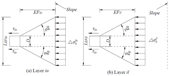
For a given layer within the upper or lower model, the soil resistance ($p_i$) is schematized in Figure 7. It is calculated as follows:

$$p_i=S_1∆{\sigma }_{hi}{L}_{EFi}+2S_2{\tau }_{i}D$$

(25)

where $L_{EFi}$ is the front width of the SW model, ${\tau }_i$ is the shear stress acting on the pile side, and $S_1$ and $S_2$ are 0.75 and 0.5 for a circular pile, respectively, and both values are 1.0 for a square pile [24].

Figure 7. Plan view of the layers iu and il.

As shown in Figure 7a, the front width of the upper model is:

$$L_{EFiu}=D+2\overline{{EF}_{iu}}tan{\phi }_m^{iu}$$

(26)

As shown in Figure 7b, the front width of the lower model is:

$$L_{EFil}=D+2\overline{{EF}_{il}}tan{\phi }_m^{il}$$

(27)

The shear stress ${\tau }_i$ is roughly evaluated by Equation (28).

$${\tau }_i=K_0{\sigma }_{3i}\mathrm{t}\mathrm{a}\mathrm{n}{\phi }_m^i{\displaystyle \frac{tan{\phi }_s}{tan\phi }}$$

(28)

where $K_0$ is the lateral soil stress coefficient, and its value is set to 1 considering the pile driving effect [25]. ${\phi }_s$ is the soil–pile interface faction angle, following the recommendations of Kulhawy [26] (see Table 2).

Table 2. Interface faction angle.

Material	Smooth	Rough
Steel	0.5$\phi$	0.9$\phi$
Concrete	0.8$\phi$	1.0$\phi$

As the load level increases, the horizontal stress change and the front width of the SW model grow continuously. This can cause the SW model to overestimate the soil resistance [14]. Therefore, the soil resistance ($p_i$) is limited by the ultimate soil resistance ($p_{ult}$), which is determined as follows [27].

$$p_{ult}=\left[\left(1-0.9\tan \theta +{\displaystyle \frac{1}{16}}{\displaystyle \frac{b}{D}}\right)0.8K_p^2+K_0\tan {\phi }_s\right]\gamma Dz$$

(29)

where $K_p^2={tan}^2\left({45}^2+\phi /2\right)$ is the passive earth pressure coefficient.

3.4. Subgrade Reaction Modulus

The pile response is obtained by solving Equation (1) using the finite difference method. The subgrade reaction modulus (k) is determined differently in two depth zones. Within the SW model depth range ($0\le z\le h_{sw}$), k is determined as:

$$k={\displaystyle \frac{p}{y}}$$

(30)

For depths below $h_{sw}$, lateral pile displacements are so small that the modulus (k) is taken as the maximum subgrade reaction modulus ($k_h$) [28]:

$$k_h=n_h{z}^{0.7}$$

(31)

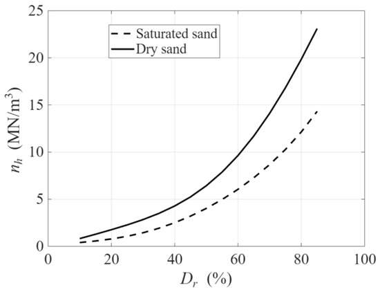
where $D_{ref}$ is 1 m, the reference diameter, and $n_h$ is the constant of the soil reaction modulus (Figure 8). Based on a series of centrifuge tests (D = 0.75~2.5, L/D = 15), Zhu et al. [28] recommended adopting the values proposed by Terzaghi [29].

Figure 8. Soil reaction modulus.

4. Verification and Discussion

4.1. Verification

(1)

Centrifuge tests

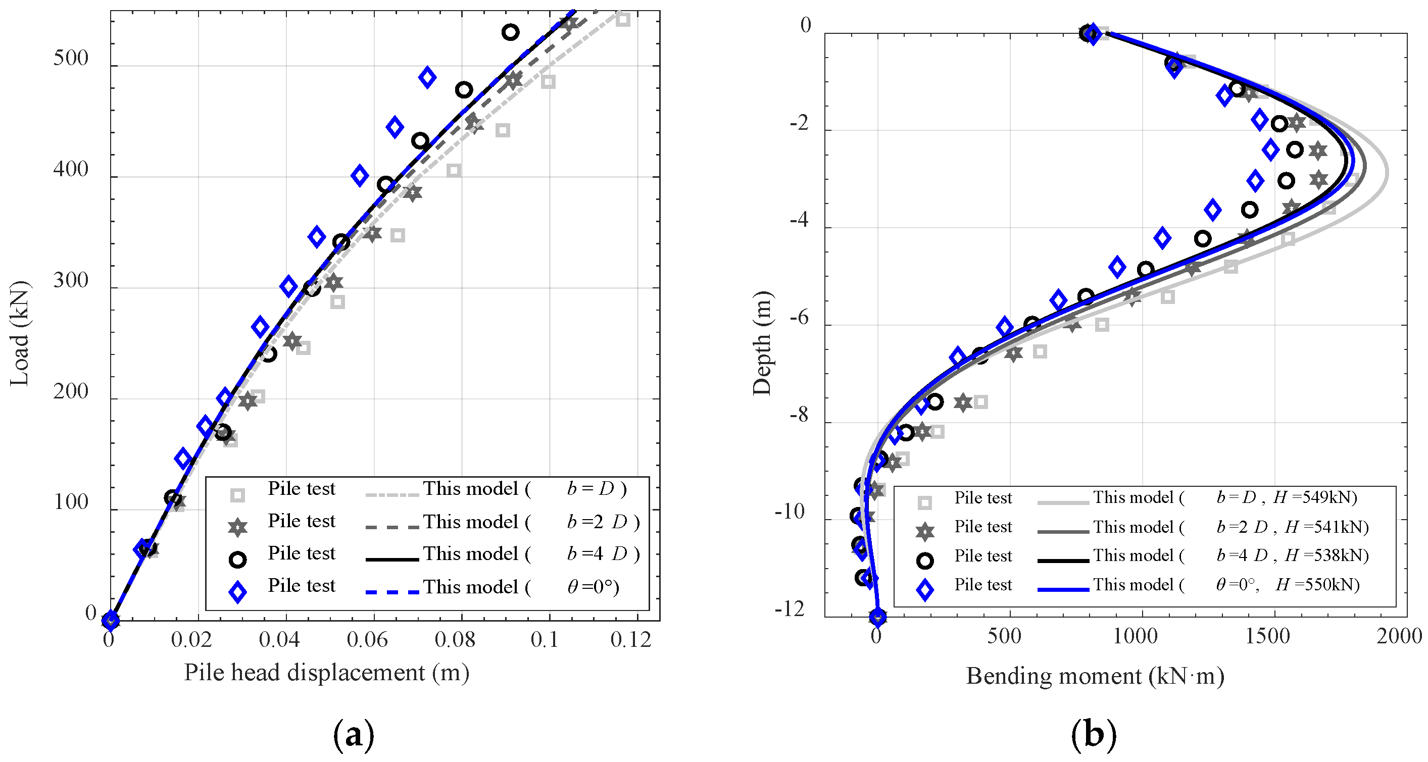
The proposed model was verified against a series of centrifuge tests reported by Mezazigh and Levacher [2]. In the tests, the lateral load was applied at a height of 1.6 m above the mudline, with 3.2 m of the pile extending above this level. The pile head displacement was measured under an incrementally increasing load. The above study did not report values for Poisson’s ratio ($\nu$) and the friction angle ($\phi$), so these parameters were determined as follows for the present analysis: $\nu$ is taken as 0.4, a representative value for sandy soils (typically ranging from 0.1 to 0.5), and $\phi$ is taken as 41$°$, based on its correlation with relative density [30]. The constant of subgrade reaction ($n_h$) is set to 20 $\mathrm{M}\mathrm{N}/{\mathrm{m}}^3$. For the hyperbolic soil stress–strain relationship, the parameters are adopted from Table 1, with $K_E$= 2000 and $R_f$= 0.6. Furthermore, as aluminum tubes were used in the experiment, the soil–pile interface friction angle is taken as 0.5$\phi$. The soil and pile properties, as well as the slope geometry, are summarized in Table 3.

Table 3. Summary of pile tests.

Slope		Soil		Pile
$\theta (°)$	b (D)	$\gamma$ (k$\mathrm{N}·{\mathrm{m}}^3$)	$D_r$ (%)	$L$ (m)	$D$ (m)	$EI$ ($\mathrm{k}\mathrm{N}·{\mathrm{m}}^2$)
26.56 0	1, 2, 4 /	16.19	81	12	0.72	514 ×${10}^3$

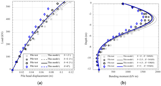
The comparison between experimental measurements and model predictions is presented in Figure 9. Specifically, Figure 9a shows the relationship between applied load and pile head displacement, while Figure 9b presents the distribution of bending moment along the pile depth. The results demonstrate that, despite minor discrepancies, the proposed method effectively captures the influence of the near-slope distance on the lateral response of the pile.

Figure 9. Pile response, (a) head displacement–load curves, (b) bending moment–depth curves.

(2)

Model tests

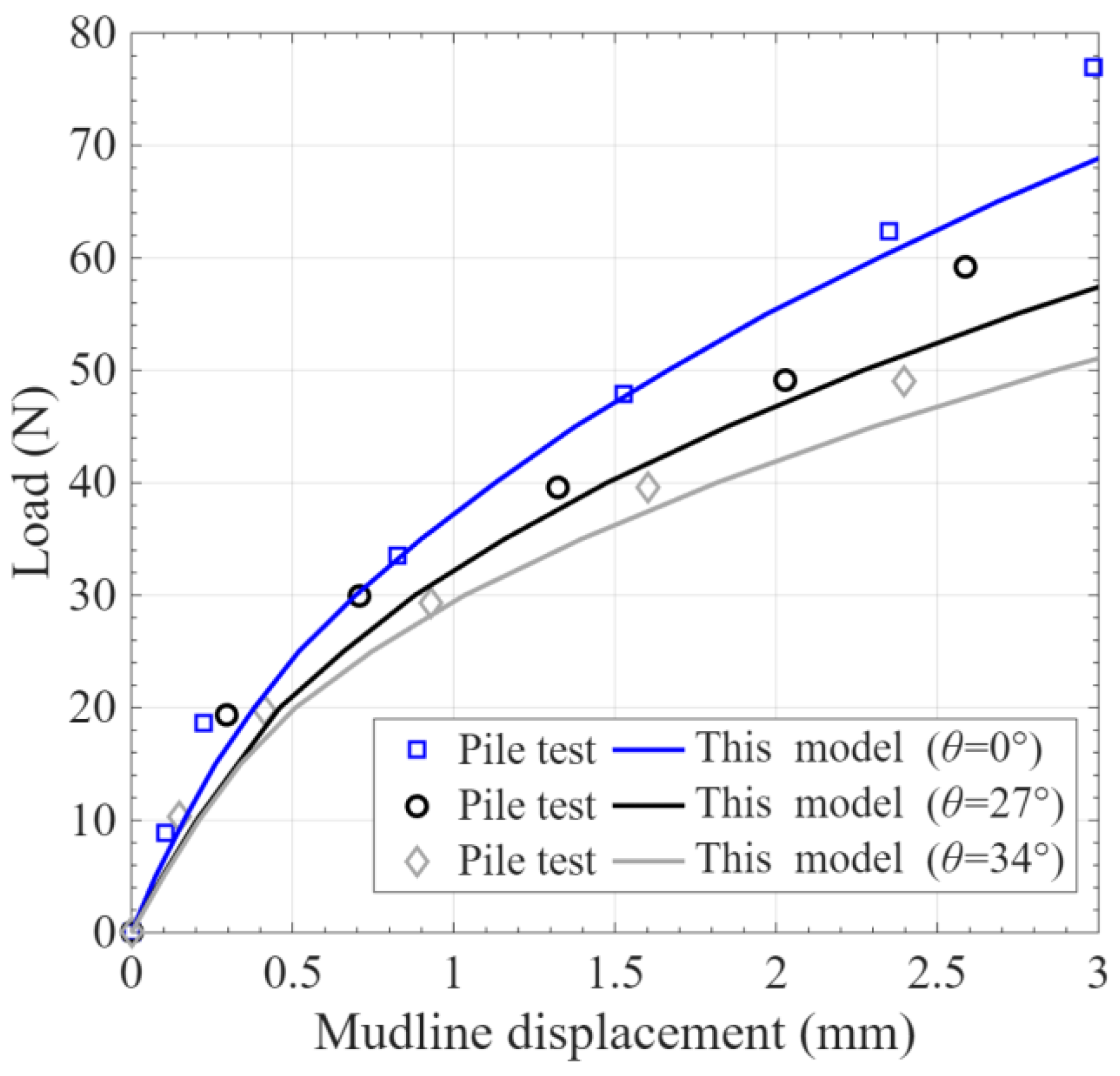
Three model tests conducted by Muthukkumaran and Almas [31] are used to verify the proposed model. In these tests, the embedded length (L) was 635 mm, the diameter (D) was 25.4 mm, and the load was applied at a height of 75 mm above the mudline. The maximum and minimum dry unit weights of the experimental sand were 19.10 $\mathrm{k}\mathrm{N}·{\mathrm{m}}^3$ and 15.19 $\mathrm{k}\mathrm{N}·{\mathrm{m}}^3$, respectively. The relative density ($D_r$) was 45%, and the friction angle (φ) was 33°. These parameters are determined as follows for the present analysis: Poisson’s ratio ($\nu$) is taken as 0.3, and the constant of subgrade reaction ($n_h$) is set to 8 $\mathrm{M}\mathrm{N}/{\mathrm{m}}^3$. For the hyperbolic soil stress–strain relationship, the parameters are $K_E$ = 400 and $R_f$ = 0.9. The soil–pile interface friction angle is taken as 0.5$\phi$. The soil and pile properties, as well as the slope geometry, are summarized in Table 4.

Table 4. Summary of model pile tests.

Soil				Pile				Slope
${\gamma }_{Max}$ ($\mathrm{k}\mathrm{N}·{\mathrm{m}}^3$)	${\gamma }_{Min}$ ($\mathrm{k}\mathrm{N}·{\mathrm{m}}^3$)	$D_r$ (%)	$\phi$ (°)	L (mm)	D (mm)	EI ($\mathrm{N}·{\mathrm{m}}^2$)	e (mm)	b (D)	θ (°)
19.10	15.19	45	33	635	25.4	287.823	75	0.5	0 26.56 33.69

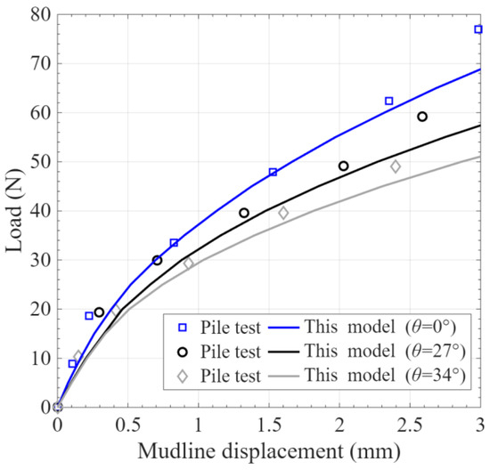
A comparison of experimental and model-predicted mudline displacement–load curves is presented in Figure 10. The model shows good agreement with test results for horizontal ground. Conversely, for piles adjacent to a slope, the proposed method yields a slight overestimation of the mudline displacement. The results demonstrate that, despite minor discrepancies, the proposed method effectively captures the influence of the slope angle on the pile response.

Figure 10. Mudline displacement–load curves.

The above verifications demonstrate that the proposed model successfully captures the influence of slope effects. This can be attributed to the consideration of three key mechanisms: the reduction in effective vertical stress, the deformation of the slope surface, and the variation in the passive soil zone width perpendicular to the loading direction.

4.2. Discussion

To investigate the influence of slope conditions on the response of the pile, slope surface, and surrounding soil, the parameters remain consistent with those from Section 4.1. The analysis primarily examines the effects of the applied load, slope angle, near-slope distance, Poisson’s ratio, and friction angle on pile displacement, bending moment, slope surface displacement, and soil deformation, where soil deformation is defined as the cumulative lateral deformation of the adjacent soil wedge.

(1)

Applied load

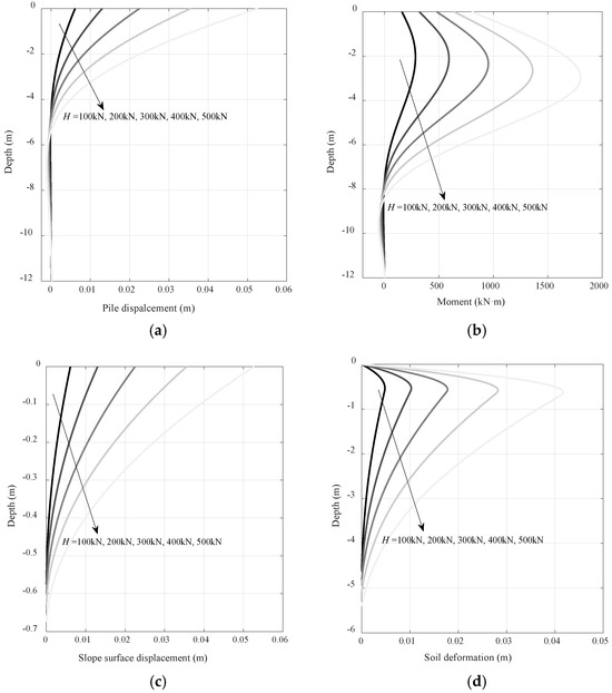
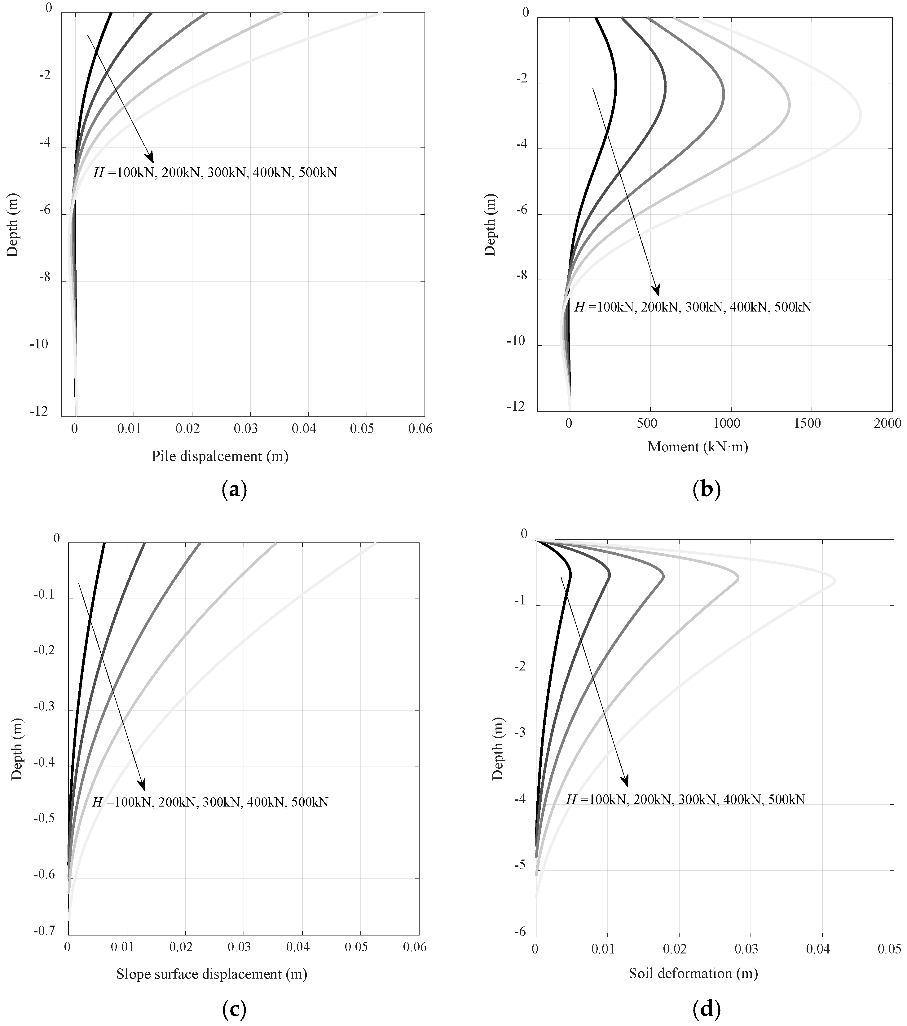
The effect of applied load on the pile response, slope surface displacement, and soil deformation is investigated for a pile at the slope crest ($\theta$ = 30°, $b$ = 0.5D), considering five load levels: H = 100 kN, 200 kN, 300 kN, 400 kN, 500 kN.

The pile response under different load levels, including lateral displacement and bending moment, is presented in Figure 11a,b, while the corresponding slope surface displacement and soil deformation distribution along the depth are presented in Figure 11c and Figure 11d, respectively. The results show that as the load increases, both the pile displacement and the corresponding depth of zero displacement gradually increase. Similarly, the magnitude of the bending moment and the depth at which the maximum bending moment occurs also increase with higher loads. The slope surface displacement decreases with depth under each load level. At a given depth, the slope surface displacement increases with the applied load. With increasing load levels, the slope surface displacement is observed to develop to greater depths. The soil deformation is zero at the mudline, increases to a maximum at a certain depth, and then decreases. At any given depth, the soil deformation exhibits a consistent increase with higher applied loads.

Figure 11. Effect of applied load, (a) pile displacement; (b) bending moment; (c) slope surface displacement; (d) soil deformation.

(2)

Slope angle

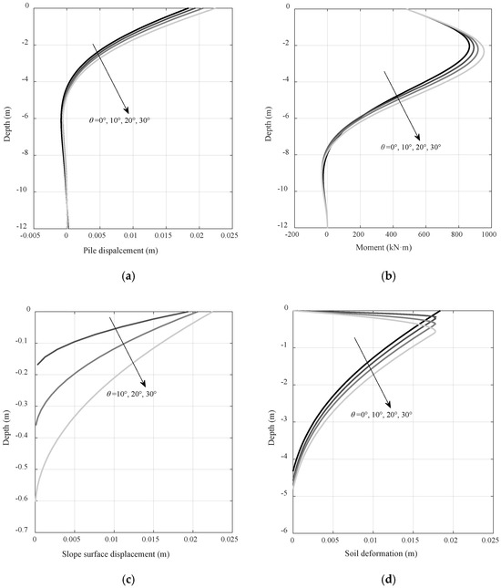
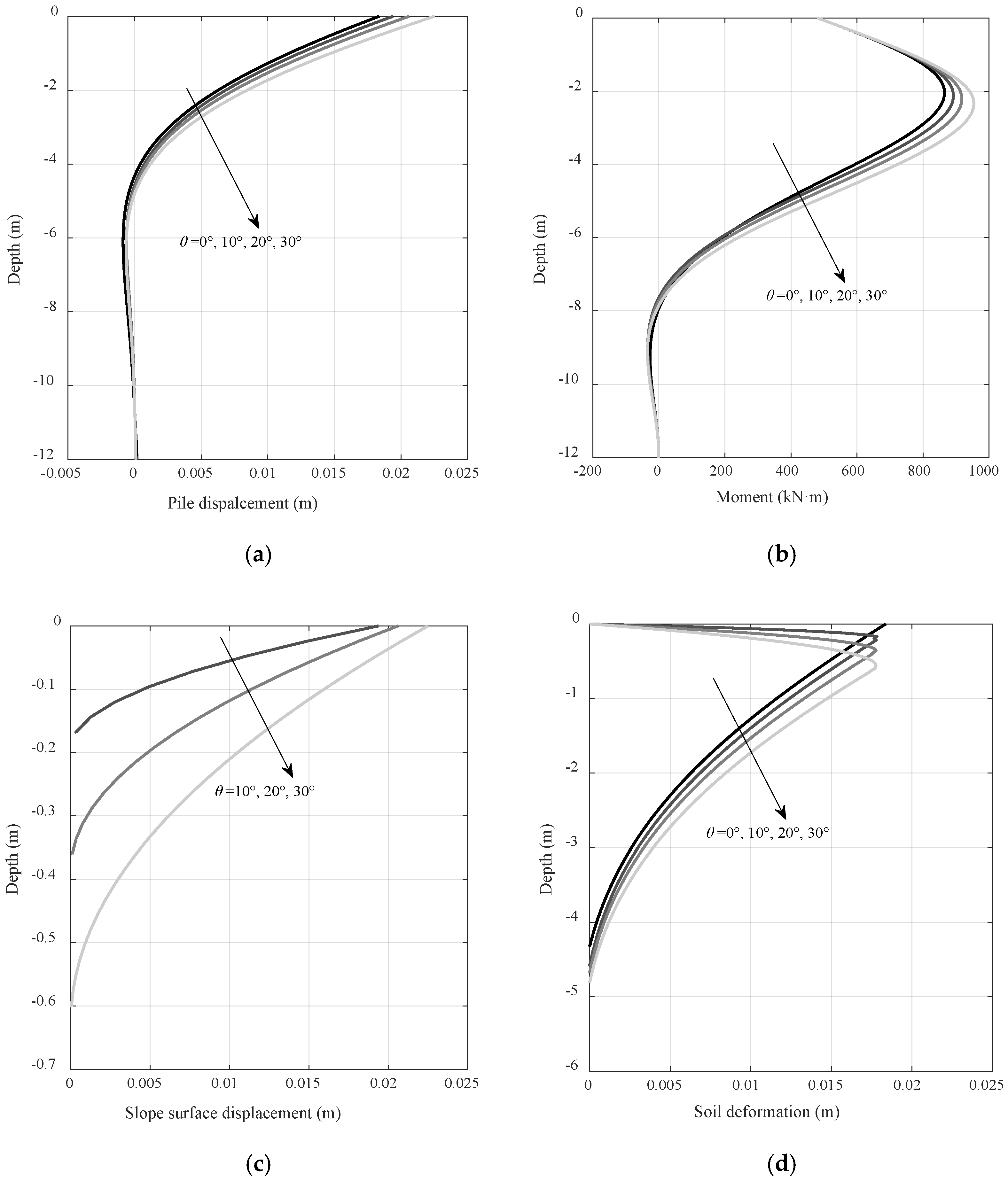
The effect of slope angle on the pile response, slope surface displacement, and soil deformation is investigated for piles installed at the crest ($b$ = 0.5D) under a constant load of H = 300 kN. Considering the stability of sandy slopes, i.e., steep slopes are prone to sliding, four slope angles are considered: $\theta$ = 0°, 10°, 20°, 30°.

The pile response under different slope angles, including lateral displacement and bending moment, is presented in Figure 12a,b, while the corresponding slope surface displacement and soil deformation distribution along the depth are presented in Figure 12c and Figure 12d, respectively. As shown in the figures, both pile displacement and bending moment increase with steeper slope angles. Correspondingly, the slope surface displacement and the depth at which it diminishes to zero also increase. Regarding soil deformation, while shallow soil exhibits reduced deformation, deeper soil shows increased deformation as the slope angle increases. This pattern occurs because a steeper slope reduces the bearing capacity of shallow soil, thereby mobilizing deeper soil to participate more actively in resisting pile deformation.

Figure 12. Effect of slope angle, (a) pile displacement; (b) bending moment; (c) slope surface displacement; (d) soil deformation.

(3)

Near-slope distance

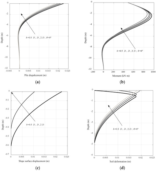
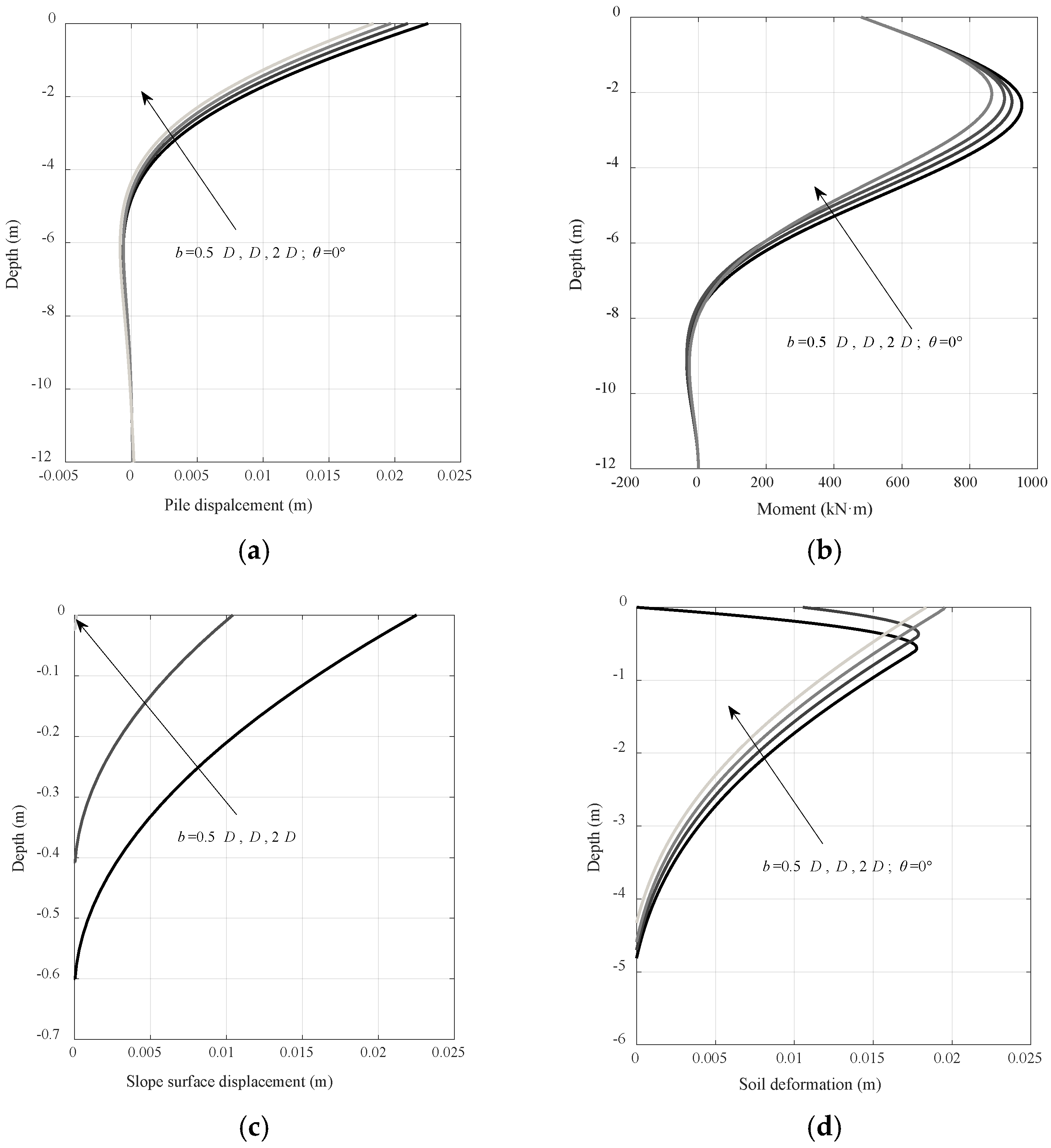
To evaluate the influence of near-slope distances, analyses are conducted for piles installed at three near-slope distances ($b$ = 0.5D, D, 2D) with an angle of $\theta$ = 30°, under a constant load of H = 300 kN.

The pile response under different near-slope distances, including lateral displacement and bending moment, is presented in Figure 13a,b, while the corresponding slope surface displacement and soil deformation distribution along the depth are presented in Figure 13c and Figure 13d, respectively. As shown in the figures, as the pile is located closer to the slope crest, both its displacement and bending moment increase. The slope surface displacement gradually increases as the near-slope distance decreases, especially near the crest. When the near-slope distance is 2D, the slope surface displacement and the depth of its occurrence become negligible. This is because the depth ($h_u$) at which the passive compression zone intersects with the slope surface is close to the mudline, making the SW model behavior essentially equivalent to that in level ground. Regarding soil deformation, shallow soil exhibits reduced deformation, while deeper soil shows increased deformation as the near-slope distance decreases. This behavior arises because reducing the near-slope distance similarly diminishes the effective bearing capacity of shallow soil, which in turn mobilizes deeper soil to provide greater resistance to pile deformation.

Figure 13. Effect of near-slope distance, (a) pile displacement; (b) bending moment; (c) slope surface displacement; (d) soil deformation.

Analyses of the compression of soil surrounding piles in sloping ground by Ng and Zhang [32] and Zhang et al. [33] showed that net compression in shallow layers decreases with increasing slope angle. These findings agree with the results presented in Figure 11d and Figure 12d, further corroborating the validity of the proposed model.

(4)

Poisson’s ratio

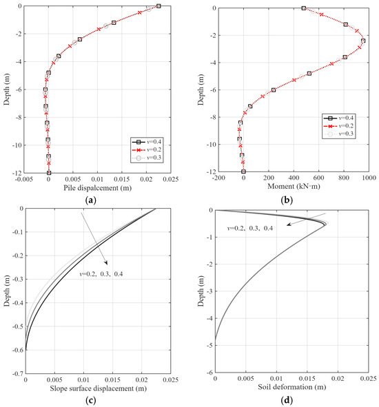
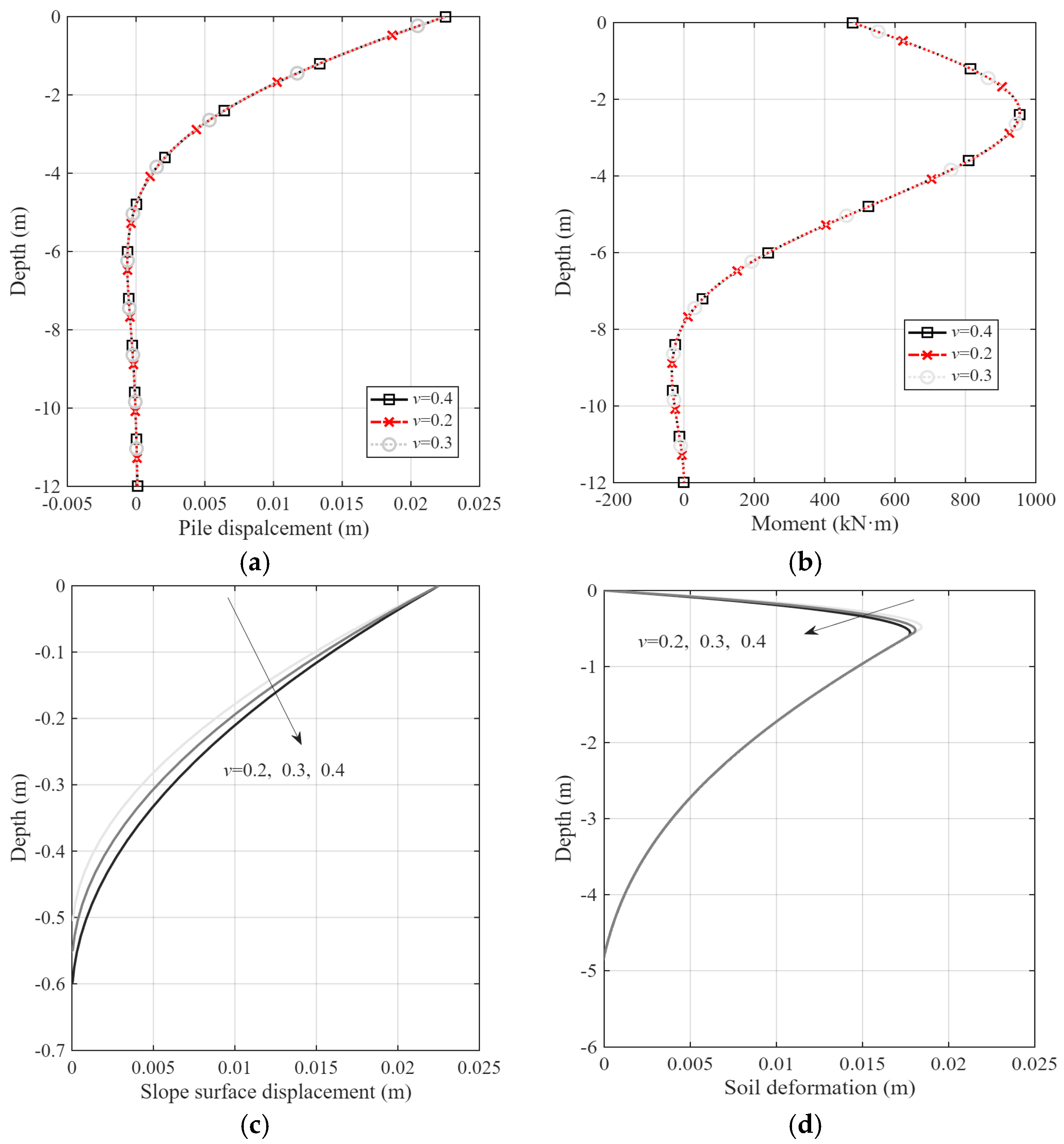
Owing to the uncertainty in determining the Poisson’s ratio of sand, a parametric study is conducted to assess its influence on the pile response, slope surface displacement, and soil deformation. The analysis considers a pile at the crest ($b$ = 0.5D, θ = 30°) under a constant load of H = 300 kN. Three values of Poisson’s ratio are considered: $\upsilon$ = 0.2, 0.3, 0.4.

The pile response under different Poisson’s ratios is presented in Figure 14a,b, while the corresponding distributions of slope surface displacement and soil deformation along the depth are presented in Figure 14c and Figure 14d, respectively. As shown in the figures, both pile displacement and bending moment are mostly unaffected by the variation in Poisson’s ratio. In contrast, the slope surface displacement and the depth to which it extends increase at higher Poisson’s ratios. Regarding soil deformation, its distribution with depth is also influenced, with a tendency for deformation to decrease in shallow layers under higher Poisson’s ratios.

Figure 14. Effect of Poisson’s ratio, (a) pile displacement; (b) bending moment; (c) slope surface displacement; (d) soil deformation.

(5)

Friction angle

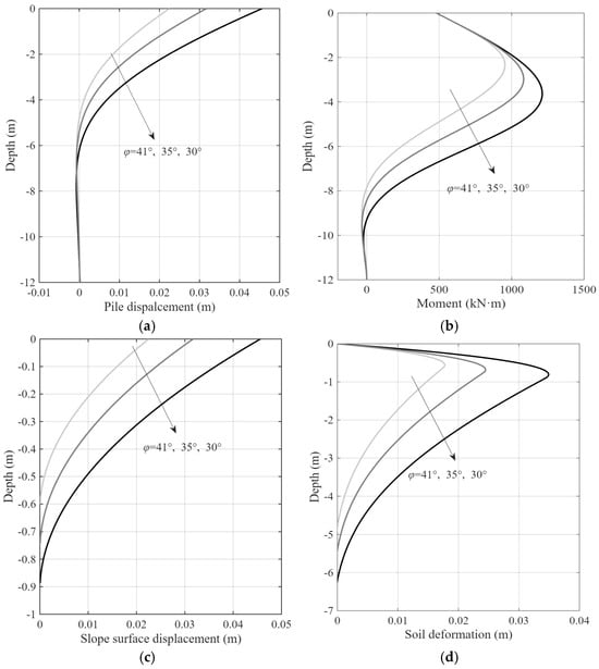
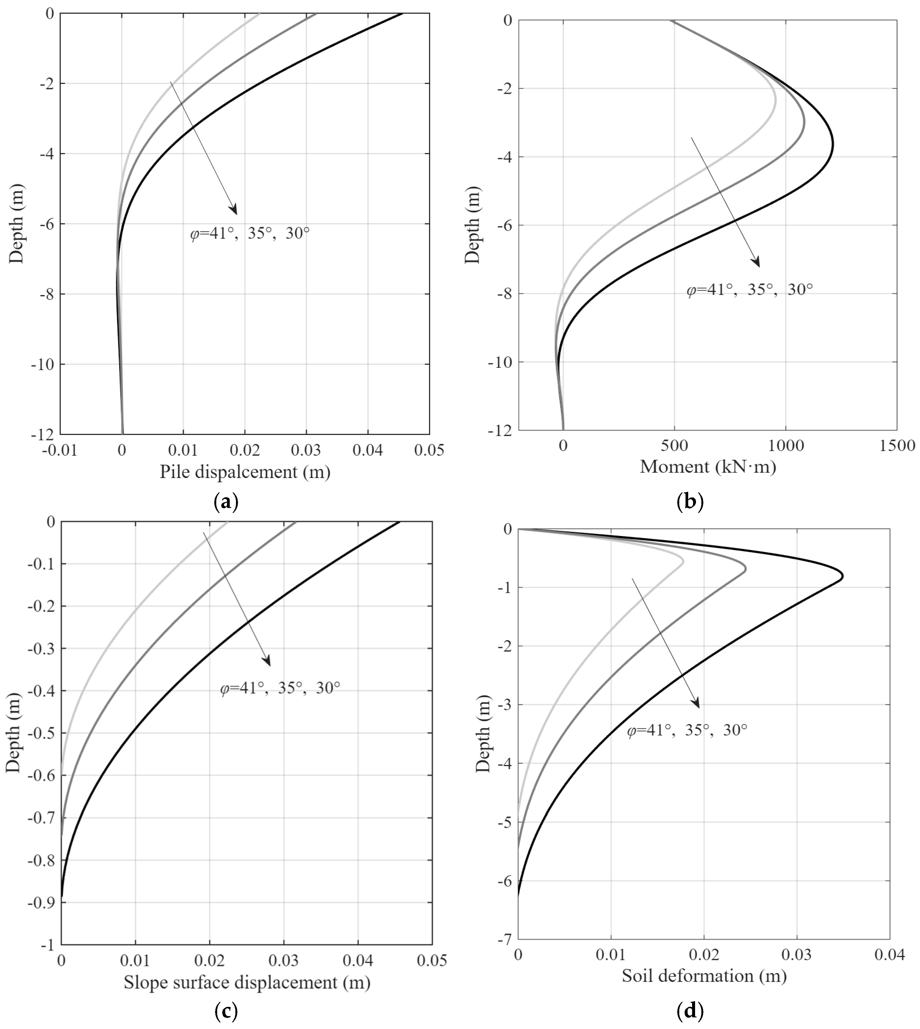
The effect of friction angle on the pile response, slope surface displacement, and soil deformation is investigated for a pile at the slope crest ($\theta$ = 30°, $b$ = 0.5 D) under a constant load of H = 300 kN. Three values of the friction angle are considered: $\phi$ = 30°, 35°, 41°.

The pile response under different friction angles, including lateral displacement and bending moment, is presented in Figure 15a,b, while the corresponding slope surface displacement and soil deformation distribution along the depth are presented in Figure 15c and Figure 15d, respectively. The results show that as the friction angle increases, both the pile displacement and the corresponding depth of zero displacement gradually decrease. Similarly, the magnitude of the bending moment and the depth at which the maximum bending moment occurs also decrease with higher friction angles. The slope surface displacement decreases with the friction angle. With decreasing friction angles, slope surface displacement is observed to develop to greater depths. At a shallow depth, the soil deformation exhibits an increase with lower friction angles.

Figure 15. Effect of friction angle, (a) pile displacement; (b) bending moment; (c) slope surface displacement; (d) soil deformation.

5. Conclusions

A nonlinear SW model for laterally loaded piles installed near sandy slopes is developed in this paper, incorporating the effects of slope surface deformation and the reduction in effective vertical stress. The main findings are summarized as follows:

(1)

The reliability of the proposed model is verified through comparisons with a series of centrifuge tests [21] and three model tests [31]. The obtained pattern of shallow soil deformation is consistent with findings reported in the previous literature, further corroborating the validity of the model.

(2)

Both the magnitude of slope surface displacement and the depth at which it diminishes to zero increase with higher load levels, steeper slope angles, smaller near-slope distances, larger values of Poisson’s ratio, and smaller friction angles. When the near-slope distance reaches 2D, the slope surface displacement becomes negligible.

(3)

Soil deformation in shallow soil decreases with increasing slope angles or decreasing near-slope distances. Conversely, deformation in deeper soil increases under the same conditions. The slope effect reduces the effective bearing capacity of shallow soil, thereby mobilizing deeper soil to provide greater resistance to pile deformation.

(4)

It is important to declare the limitation that this model is valid solely for gentle slopes without a sliding surface.

References

- Nimityongskul, N.; Kawamata, Y.; Rayamajhi, D.; Ashford, S.A. Full-scale tests on effects of slope on lateral capacity of piles installed in cohesive soils. J. Geotech. Geoenviron. Eng. 2018, 144, 04017103. [Google Scholar] [CrossRef] [Scilit]
- Mezazigh, S.; Levacher, D. Laterally loaded piles in sand: Slope effect on p-y reaction curves. Can. Geotech. J. 1998, 35, 433–441. [Google Scholar] [CrossRef]
- Rathod, D.; Muthukkumaran, K.; Thallak, S. Experimental investigation on behavior of a laterally loaded single pile located on sloping ground. Int. J. Geomech. 2019, 19, 04019021. [Google Scholar] [CrossRef] [Scilit]
- Yang, M.; Deng, B.; Wang, Y. A simplified calculation method for the near-slope laterally loaded pile based on a passive wedge model. Adv. Civ. Eng. 2019, 2019, 8363252. [Google Scholar] [CrossRef] [Scilit]
- Chen, L.; Jiang, C.; Pang, L.; Liu, P. Lateral soil resistance of rigid pile in cohesionless soil on slope. Comput. Geotech. 2021, 135, 104163. [Google Scholar] [CrossRef] [Scilit]
- Lin, M.; Jiang, C.; Chen, Z.; Liu, P.; Pang, L. A method for calculating lateral response of offshore rigid monopile in sand under slope effect. Ocean Eng. 2022, 259, 111812. [Google Scholar] [CrossRef] [Scilit]
- Jiang, C.; Liu, J.; Lin, M. Study Method of Pile near Cohesionless Slope under Reversed Lateral Load Considering Sand Strength State and Lateral Deflection of Pile. J. Mar. Sci. Eng. 2023, 11, 741. [Google Scholar] [CrossRef] [Scilit]
- Georgiadis, K.; Georgiadis, M. Undrained Lateral Pile Response in Sloping Ground. J. Geotech. Geoenviron. Eng. 2010, 136, 1489–1500. [Google Scholar] [CrossRef] [Scilit]
- Georgiadis, K.; Georgiadis, M. Development of p–y curves for undrained response of piles near slopes. Comput. Geotech. 2012, 40, 53–61. [Google Scholar] [CrossRef] [Scilit]
- Sun, B.; Jiang, C.; Pang, L.; Liu, P.; Li, X. Effect of the pile diameter and slope on the undrained lateral response of the Large–Diameter pile. Comput. Geotech. 2022, 152, 104981. [Google Scholar] [CrossRef] [Scilit]
- Pang, L.; Jiang, C.; Chen, L. Nonlinear Predictive Framework of the Undrained Clay Slope Effect on the Initial Stiffness of p-y Curves of Laterally Loaded Piles by FEM. J. Mar. Sci. Eng. 2022, 10, 1684. [Google Scholar] [CrossRef] [Scilit]
- Wang, Y.; Chen, J.; Pan, Z.; Yang, L.; Zhang, H.; Wu, X. Experimental Study on Horizontal Resistance Parameter of Gravelly Soil Considering Slope Gradient Factor. Buildings 2024, 14, 3346. [Google Scholar] [CrossRef] [Scilit]
- Norris, G. Theoretically based BEF laterally loaded pile analysis. In Proceedings of the 3rd International Conference on Numerical Methods in Offshore Piling, Navtes, France, 21–22 May 1984. [Google Scholar]
- Ashour, M.; Norris, G.; Pilling, P. Lateral loading of a pile in layered soil using the strain wedge model. J. Geotech. Geoenviron. Eng. 1988, 124, 303–315. [Google Scholar] [CrossRef] [Scilit]
- Yang, X.; Zhang, C.; Huang, M.; Yuan, J. Lateral loading of a pile using strain wedge model and its application under scouring. Mar. Georesour. Geotechnol. 2018, 36, 340–350. [Google Scholar] [CrossRef] [Scilit]
- Peng, W.; Zhao, M.; Xiao, Y.; Yang, C.; Zhao, H. Analysis of laterally loaded piles in sloping ground using a modified strain wedge model. Comput. Geotech. 2019, 107, 163–175. [Google Scholar] [CrossRef] [Scilit]
- Hemel, M.; Korff, M.; Peters, D. Analytical model for laterally loaded pile groups in layered sloping soil. Mar. Struct. 2022, 84, 103229. [Google Scholar] [CrossRef] [Scilit]
- Qian, Z.; Lu, X.; Yang, W. Comparative Field Tests on Straight-Sided and Belled Piers on Sloping Ground under Combined Uplift and Lateral Loads. J. Geotech. Geoenviron. Eng. 2019, 145, 04018099. [Google Scholar] [CrossRef] [Scilit]
- Jiang, C.; Sun, M.; Liu, P.; Lin, M.; Liu, J. Analytical method for laterally loaded offshore slender piles near sandy slopes considering slope deformation. Mar. Georesour. Geotechnol. 2024, 43, 383–395. [Google Scholar] [CrossRef] [Scilit]
- Liu, P.; Jiang, C. A new p–y curve criterion for piles in proximity to undrained clay slopes. Comput. Geotech. 2023, 164, 105801. [Google Scholar] [CrossRef] [Scilit]
- Liu, P.; Jiang, C. A modified p-y curve model for offshore piles near sandy slopes considering the soil-pile-slope deformation mechanism. Mar. Struct. 2024, 98, 103675. [Google Scholar] [CrossRef] [Scilit]
- Duncan, J.; Chang, C. Nonlinear analysis of stress and strain in soils. J. Soil Mech. Found. Div. 1970, 96, 1629–1653. [Google Scholar] [CrossRef] [Scilit]
- Byrne, P.; Cheung, H.; Yan, L. Soil parameters for deformation analysis of sand masses. Can. Geotech. J. 1988, 24, 366–376. [Google Scholar] [CrossRef] [Scilit]
- Briaud, J.; Smith, T.; Meyer, B. Laterally loaded piles and the pressuremeter: Comparison of existing methods. In Laterally Loaded Deep Foundations: Analysis and Performance; ASTM International: West Conshohocken, PA, USA, 1984; pp. 74–111. [Google Scholar] [CrossRef] [Scilit]
- Xu, L.-Y.; Cai, F.; Wang, G.-X.; Ugai, K. Nonlinear analysis of laterally loaded single piles in sand using modified strain wedge model. Comput. Geotech. 2013, 51, 60–71. [Google Scholar] [CrossRef] [Scilit]
- Kulhawy, F. Limiting tip and side resistance: Fact or fallacy? In Analysis and Design of Pile Foundations; ASCE: Reston, VA, USA, 1984; pp. 80–98. [Google Scholar]
- Gao, B.; Zhang, C.; Zhang, Z. Model tests on effect of slopes on lateral resistance of near single piles in sand. Rock Soil Mech. 2014, 35, 3191–3198. [Google Scholar] [CrossRef]
- Zhu, B.; Li, T.; Xiong, G.; Liu, J.C. Centrifuge model tests on laterally loaded piles in sand. Int. J. Phys. Model Geotech. 2016, 16, 160–172. [Google Scholar] [CrossRef] [Scilit]
- Terzaghi, K. Evaluation of coefficient of subgrade reaction. Géotechnique 1955, 5, 297–326. [Google Scholar] [CrossRef] [Scilit]
- Mujtaba, H.; Farooq, K.; Sivakugan, N.; Das, B.M. Evaluation of relative density and friction angle based on SPT-N values. KSCE J. Civ. Eng. 2018, 22, 572–581. [Google Scholar] [CrossRef] [Scilit]
- Muthukkumaran, K.; Almas, B. Experimental investigation of single model pile subjected to lateral load in sloping ground. Geotech. Geol. Eng. 2015, 33, 935–946. [Google Scholar] [CrossRef] [Scilit]
- Ng, C.; Zhang, L. Three-dimensional analysis of performance of laterally loaded sleeved piles in sloping ground. J. Geotech. Geoenviron. Eng. 2001, 127, 499–509. [Google Scholar] [CrossRef] [Scilit]
- Zhang, L.; Ng, C.; Lee, C. Effects of slope and sleeving on the behavior of laterally loaded piles. Soils Found. 2004, 44, 99–108. [Google Scholar] [CrossRef] [Scilit]
Disclaimer/Publisher’s Note: The statements, opinions and data contained in all publications are solely those of the individual author(s) and contributor(s) and not of MDPI and/or the editor(s). MDPI and/or the editor(s) disclaim responsibility for any injury to people or property resulting from any ideas, methods, instructions or products referred to in the content. |
© 2026 by the authors. Licensee MDPI, Basel, Switzerland. This article is an open access article distributed under the terms and conditions of the Creative Commons Attribution (CC BY) license.