


Abstract
The construction industry has a higher accident rate than other industries and a shrinking inflow of new workers, and obstacle avoidance is a core task for autonomous construction equipment. Many earlier studies treated every obstacle as a single category with an identical penalty, which limits their use on real sites. This study proposes a deep reinforcement learning (DRL) reward function that reflects the quantitative criteria of construction safety regulations. RecurrentPPO, combining Proximal Policy Optimization (PPO) with Long Short-Term Memory (LSTM), served as the local planner and Hybrid A* as the global planner. From KOSHA GUIDE C-48-2022 and the Rules on Occupational Safety and Health Standards, type-specific obstacle penalties, a four-zone safety-distance scheme and speed terms were designed. Three groups and three reward ablations were compared in simulation. Against a baseline reward with a single safety-distance term, the difference in success rate (71.2% vs. 58.9%) was not statistically significant, and the drop in collision rate from 41.0% to 25.1% was significant in Welch’s t-test but only marginal in the Mann–Whitney U test. The proposed reward had its clearest effect near workers. The share of steps above the 10 km/h limit fell from 90.9% to 51.5%, and worker collisions were halved. A safety-regulation-based reward thus mainly shapes regulation-consistent driving rather than raising the arrival rate.
1. Introduction
An earthwork field and similar construction sites are spaces where the environment changes in real time and where many machines, vehicles, and workers operate together, so various accidents arise during the work process. In particular, collisions with obstacles or workers have kept occurring as transport vehicles carrying materials and construction machines such as rollers and dozers move around the site. To tackle this problem, the Korea Occupational Safety and Health Agency (KOSHA) enacted KOSHA GUIDE C-48-2022 [1] and has encouraged workers to observe the regulation on site. In addition, the Ministry of Employment and Labor’s Rules on Occupational Safety and Health Standards [2], which stand above the KOSHA GUIDE in the regulatory hierarchy, prescribe operating criteria and separation distances for mobile equipment and limit the speed of vehicles moving on site, thereby working from an institutional standpoint to prevent accidents. Yet the complex nature of construction sites makes thorough compliance difficult, and the subjective view of the person in charge often enters into judgments about whether the rules have been observed, so a technical solution is called for.
Introducing autonomous driving to construction equipment has emerged as one such solution, and it is also discussed as a response to the shrinking and aging on-site workforce. Deep reinforcement learning (DRL) has been studied actively for the real-time avoidance of dynamic obstacles in complex environments that were not observed beforehand. Most of this work has targeted autonomous driving for vehicles on ordinary roads, and cases applied to complex and irregular environments such as construction sites remain rare. Many prior studies also treat obstacles as a single category and assign the same penalty to all of them, which is hard to apply to the complex environment of an actual site. Moreover, to our knowledge, few studies have directly reflected the quantitative criteria of safety regulations, an institutional instrument, in a DRL reward function.
This study aims to fuse the quantitative criteria of construction safety regulations with a reward function in mathematical form so as to shape collision-avoidance behavior that follows the regulations and to examine its effect on the learning stability of DRL. To validate the newly designed reward function, we build a two-layer hybrid structure that couples global path planning based on the Hybrid A* algorithm with local path planning based on RecurrentPPO, which combines Proximal Policy Optimization (PPO) with Long Short-Term Memory (LSTM). Within this setting we present a baseline reward function and the proposed reward function, divide the experiment into three groups through variable control, and evaluate the effect of the proposed reward through comparative testing in a simulation environment. Compared with the baseline, the proposed reward did not significantly change the success rate but mainly changed how the agent drove near hazards, lowering its speed and keeping it farther from workers. The two-layer structure proved to be a prerequisite for either reward to work.
2. Theoretical Background and Related Work
2.1. Path Planning and Deep Reinforcement Learning
Global path planning provides a route that reaches the goal from the start point while avoiding static obstacles, and the A* algorithm has been a representative technique for this purpose. Hart et al. [3] proposed A* as a heuristic graph search that efficiently finds a minimum-cost path, but because it is typically applied on a grid it has trouble reflecting the actual motion of a vehicle. Dolgov et al. [4] proposed the Hybrid A* algorithm, which keeps the grid-based search structure while tracking at each node continuous coordinates that follow a kinematic model of the vehicle, so that the resulting path is guaranteed to be drivable even in unknown semi-structured environments. It was therefore adopted as the global path-planning algorithm in this study.
For local path planning, which must respond to and avoid dynamic obstacles that move in real time, deep reinforcement learning is well suited. In the framework of Sutton and Barto [5], an agent learns a policy that maximizes cumulative reward through repeated interaction with the environment, which enables avoidance, even without prior information. Mnih et al. [6] combined a deep network with this framework in the Deep Q-Network (DQN) and showed that a value function can be approximated for high-dimensional state spaces. The PPO proposed by Schulman et al. [7] is a practical improvement over the computationally expensive Trust Region Policy Optimization (TRPO) [8]; by limiting the extent of policy updates through a clipping technique, it raises learning stability and lowers sensitivity to hyperparameters. Because a LiDAR sensor cannot fully observe the surrounding environment, information from earlier time steps must also be used. Hochreiter and Schmidhuber [9] proposed LSTM to solve the long-term dependency problem of recurrent networks, and Hausknecht and Stone [10] showed that replacing a fully connected layer of DQN with an LSTM lets the Deep Recurrent Q-Network (DRQN) integrate information over time and hold its performance better when observations become incomplete.
2.2. Obstacle Avoidance on Construction Sites and Deep Reinforcement Learning
Efforts to prevent construction-site accidents through automation have been pursued in many directions. Ahammed et al. [11] developed a computer-vision model that detects road obstacles in construction zones for autonomous cars and reported high detection accuracy under diverse conditions. Wickberg et al. [12] analyzed the dynamic-map requirements arising from the complex characteristics of construction sites and showed that a mapping approach different from that of ordinary roads is required. The choice of agent model also matters. Kwiatkowski et al. [13] showed that even under identical conditions the choice between holonomic and nonholonomic control significantly changes learning performance and efficiency. Because the motion model can shape the results this strongly, we fixed a simplified kinematic model without acceleration limits across all groups so that the effect of the reward function could be isolated.
As research on DRL-based obstacle avoidance has continued, effective avoidance has been demonstrated in ever more complex environments. Duan and Zou [14] improved collision avoidance in construction-robot manipulation with a trust-region method that imposes collision risk as a conditional value-at-risk constraint instead of an expectation-based one. Poudel et al. [15] combined Simultaneous Localization and Mapping (SLAM) with a transformer-based Twin Delayed Deep Deterministic policy gradient (TD3) to improve dynamic obstacle avoidance for autonomous construction robots. Zhu and Zhang [16] reviewed DRL-based mobile-robot navigation and confirmed that DRL adapts better than conventional rule-based approaches in complex environments. Zhang et al. [17] added an Intrinsic Curiosity Module and an LSTM to PPO and showed in Gazebo and on a TurtleBot3 robot that the intrinsic reward speeds up convergence under sparse rewards while the LSTM improves the avoidance of dynamic obstacles. Everett et al. [18] used an LSTM to learn collision avoidance among a varying number of heterogeneous pedestrians and robots without assuming that they follow any particular behavior rules. Luo et al. [19] confirmed with an LSTM-PPO algorithm that time-series processing raises learning stability in continuous action spaces.
Research on construction automation has also moved toward autonomous equipment on site. Melenbrink et al. [20] reviewed on-site construction robots and found that industry efforts have concentrated on adding autonomy to conventional earthmoving equipment, while the chaotic conditions of construction sites remain the main obstacle to full autonomy. Zhang et al. [21] deployed an autonomous excavator that fuses LiDAR and camera data for perception and combines learning-based and optimization-based planning, and the system operated for 24 h without human intervention; its safety relied on a predefined operating region and an immediate stop when a person was detected. Safety between workers and moving equipment has been studied mainly as a sensing problem. Teizer et al. [22] tested a radio-frequency proximity warning system in which tags worn by workers and units mounted on equipment trigger alarms when the two come too close, and Kim et al. [23] predicted the future proximity between a worker and a truck from UAV imagery with deep neural networks so that alerts and rerouting can be issued in advance. These studies detect or predict hazardous proximity and leave the decision on how to drive to an operator or a separate planner. None of them builds the separation and speed requirements of safety regulations into the learning objective of an autonomous vehicle, which is the gap addressed in this study.
2.3. Construction Safety Regulations and Reward Function Design
The core task of this study is to reflect construction safety regulations, an institutional instrument, in an algorithm in mathematical form. KOSHA GUIDE C-48-2022 [1] and the higher-ranking Rules on Occupational Safety and Health Standards [2] set out on-site deceleration duties, the extent of no-entry zones, site-specific speed limits, and approach-restriction distances as rules meant to prevent accidents. Because workers and equipment frequently share the same space, items dealing with contact between equipment and pedestrians were mainly adopted. With German in-depth crash data, Rosén and Sander [24] showed that the fatality risk of adult pedestrians struck by the front of a car follows a logistic curve of impact speed, and Tefft [25] extended this analysis to severe injury and to light trucks using US data. Although both studies concern passenger cars and light trucks rather than construction machines and report low absolute risks at low speeds, they show that the risk keeps rising steadily with every increase in speed, which supports holding speed down near workers.
How these criteria are converted into mathematical form depends on the reward-function design of the DRL. Krautwig et al. [26] quantitatively analyzed how the weighting of reward terms governs the trade-off between fast arrival and collision avoidance in maritime autonomous navigation, and Taheri et al. [27] showed that an enhanced PPO combined with a carefully designed reward function improves safe mobile-robot navigation. Arvind and Senthilnath [28] trained an MLP-SARSA agent in a Pygame urban scenario containing road-following and randomly moving obstacles, yet every crash received the same penalty of −500 whether it involved an obstacle or a road border, even though the two were counted separately in evaluation. Alsuwaiket [29] classified pedestrians, vehicles and cyclists in perception, yet the reward penalized collisions through a single probability term whose weight changed with the traffic context rather than with the type of road user. Hu [30] designed a scenario-adaptive multi-objective reward for PPO-based driving decisions but reported that the policy remained unstable in extremely complex traffic.
3. Materials and Methods
3.1. Research Framework and Experimental Design
This study is carried out by combining design-science research with performance verification in a simulation environment. We analyze construction safety regulations, design a new reward function from the quantified criteria, and implement the two-layer hybrid path planning and the virtual environment in Python. The overall system architecture and research framework are shown in Figure 1. Three groups are set up through the variables, and their performance is verified through comparative experiments in simulation.
Figure 1.
System architecture and research framework of the proposed two-layer hybrid obstacle-avoidance model.
Two variables are used to separate the groups: the type of reward function and the path-planning layer. The three groups obtained through variable control are listed in Table 1. Single-layer path planning refers to path planning without the Hybrid A* algorithm, which serves as the global planner; every group was otherwise tested in an identical environment.
Table 1.
Experimental group configurations.
A two-dimensional environment based on Gymnasium and Pygame is built, and a simplified kinematic model is adopted as the motion model of the agent so that physical conditions other than the designed variables do not interfere with the results. The workspace emulates a square medium-scale earthwork site of 200 m × 200 m and is rendered at 800 × 800 pixels (1 px = 0.25 m). The start point is (84 m, 20 m), the goal point is (100 m, 170 m), one time step is 0.1 s, and each episode is capped at 2000 steps. As shown in Figure 2, the layout lets the agent encounter every type of obstacle as it moves from the start point to the goal, which prevents excessive learning of any single obstacle. Obstacles are divided into static obstacles that stay fixed and dynamic obstacles that move in a regular or irregular manner; construction equipment and vehicles show regular movement, unexpected obstacles are generated and removed probabilistically, and workers move back and forth between two points, with noise added to reflect actual human motion.
Figure 2.
Layout of the two-dimensional Gymnasium/Pygame simulation testbed emulating a medium-scale earthwork site.
The agent represents a transport vehicle with a 2.5 m × 5.0 m footprint and is treated as a circle of radius 2.8 m for collision checking. Its motion follows a simplified unicycle model. At each step the policy outputs a speed command in [0, 3.0] m/s and a heading change in [−0.5, 0.5] rad, which are applied directly without acceleration limits. The observation is a 41-dimensional vector made up of 36 LiDAR range readings spaced 10° apart with a maximum range of 15 m and five state values: the distance and relative angle to the current target, the agent’s speed, and the sine and cosine of its heading. The current target is the next Hybrid A* waypoint in Groups A and B and the goal itself in Group C. The type label is therefore needed only to compute the reward during training in simulation. At deployment the policy acts on the range readings and the five state values alone, so no obstacle classification is required to run it. This follows the common practice of training in simulation with a reward that uses information unavailable to the agent, and its consequences for the learned behavior are discussed in Section 4.4 and Section 4.7. Workers walk at 1.2 m/s with Gaussian positional noise (σ = 0.15 m per step); vehicles and equipment patrol 30 m segments at 2.0 m/s and 0.5 m/s; and unexpected obstacles appear at one of seven fixed points with a probability of 0.025 per step, with at most three present at a time, and vanish after 8 s.
Three Python modules were implemented for the deep reinforcement learning. construction_env.py builds a Gymnasium-compatible custom environment that holds the agent, LiDAR ray casting, the reward function, and the placement of static and dynamic obstacles, and supports Pygame-based visualization. hybrid_astar.py implements the Hybrid A* global planner: it searches an (x, y, θ) state space discretized with a grid resolution of 2.0 m and 36 heading directions, applies a 4.0 m inflation radius to static obstacles, expands nodes with a 3.0 m step size using five steering angles as motion primitives, and extracts waypoints at least 8 m apart along the path that the agent follows in sequence. train.py supports training, validation, and demonstration with RecurrentPPO from the SB3-Contrib library and automatically logs per-episode metrics to CSV.
The main hyperparameters of the training algorithm are listed in Table 2. Sixteen parallel environments were configured with SubprocVecEnv to shorten training time, and observations were normalized with VecNormalize while rewards were left unnormalized. This choice was deliberate. The reward signal combines sparse terminal rewards, such as the goal reward (+100) and the collision penalties (−100 and the like), with dense per-step rewards, and these two families operate on very different scales. When running reward normalization is applied, the normalizer rescales the reward signal dynamically as training proceeds, so the relative scale between the sparse safety-critical rewards and the dense path-efficiency rewards becomes distorted after the middle of training. Under this reward distortion the agent was observed to over-prioritize path optimization over safety and the policy collapsed, so reward normalization was disabled. The total number of training steps was set to 1,000,000. The formulations of both algorithms, as implemented in this study, are given in Appendix A.
Table 2.
Training hyperparameters.
3.2. Baseline Reward Function
The baseline reward function for comparison was designed as the sum of six components.
and denote reaching the goal and collision; they carry the strongest reward (+100) and penalty (−100) and end the episode. drives the agent toward the goal and is computed from the change in goal distance between the previous and current step, i.e.,
while imposes a per-step penalty (−) so that the goal is reached quickly, and keeps the agent at least a safe distance from obstacles.
In Groups A and B, the agent also receives a waypoint bonus () of +5 each time it comes within 5 m of the current waypoint, after which the next waypoint becomes the target; Group C, which has no global planner, receives no such bonus.
The tuning parameters were set to = 5.0, = 0.015, and = 3.0, with m. = 5.0, multiplied by the maximum travel distance of 0.3 m per step, yields 1.5 and makes clear that preventing a collision takes priority even if all steps are consumed; = 0.015 keeps the accumulated time penalty within 30% of the arrival or collision reward even when all 2000 steps are used; and = 3.0 sets the worst-case safety penalty to −3, the largest value apart from arrival and collision, preserving the intended hierarchy among the components. Here, is the surface-to-surface distance between the agent and the nearest obstacle, obtained by subtracting the collision radius of the agent (2.8 m) from the distance between the agent’s center and the obstacle surface. therefore begins to act 3.0 m before contact and reaches its maximum of −3 at contact, and it follows the same distance convention as the proposed reward in Section 3.3.
3.3. Proposed Reward Function
A new reward function was designed by reflecting the quantitative values extracted from KOSHA GUIDE C-48-2022 [1] and the higher-ranking Rules on Occupational Safety and Health Standards [2]. Article 98 of the Rules obliges employers to set a site-specific speed limit for construction machinery whose maximum speed exceeds 10 km/h and obliges operators to observe it, and this 10 km/h threshold was adopted as the speed baseline; Article 200 prohibits workers from entering places where they could be struck by operating construction machinery, and Article 322 requires vehicles and machines to keep at least 3 m from live power lines up to 50 kV, while KOSHA GUIDE C-48-2022 requires machines to slow down when crossing obstacles and to keep at least 2 m from power lines when passing beneath them. Obstacles were reclassified into four types according to the expected severity of damage on collision and the difficulty of avoidance: workers (W) and unexpected obstacles (U) as the highest risk, vehicles (V) as high risk, and static obstacles (S) as moderate risk. Workers were set as the highest risk because the probability of human casualty is very high, and unexpected obstacles likewise because they are the hardest to avoid. Because the regulations do not prescribe zone radii for each obstacle type directly, the radii were set by combining the regulatory criteria with the physical characteristics of each type. Article 200 gives no distance for the contact-hazard zone, so the critical radius of workers was set at 2.0 m, below the width of the simulated dump truck (2.5 m × 5.0 m), as a clearance within which little room is left to avoid contact. The critical radius of vehicles (3.0 m) accounts for the agent and the other machine both being larger than a worker, and their warning radius (6.0 m) was set larger than that of workers to allow for two machines approaching each other at up to the 10 km/h limit. For static obstacles no quantitative rule on structures exists, so power lines were taken as a representative fixed structure on construction sites and the 3 m clearance from live power lines in Article 322 was applied as their warning radius. No rule exists for unexpected obstacles either, so their zones were set wider than those of workers because such obstacles appear without warning and leave the least time to react. The resulting radii are summarized per obstacle type in Figure 3.
Figure 3.
Multi-zone safety schema per obstacle type (W, V, S, U). Concentric critical, warning, caution, and safe zones are shown with their radii.
The reward function of the proposed model adds a speed component to the baseline.
was added, was differentiated by obstacle type (−100 for workers and unexpected obstacles, −80 for vehicles, and −60 for static obstacles), and the safe distance of () was subdivided into four zones: safe, caution, warning, and critical. Denoting the obstacle type by k, the surface-to-surface distance between the agent and the obstacle by d, and the agent’s speed by v, the safety penalty is defined piecewise. At d = 0 a collision penalty is imposed and the episode ends. Within the critical zone (d < ) a fixed penalty () is multiplied by the speed factor to produce a strong avoidance signal without ending the episode. In the warning zone ( ≤ d < ) an exponential decay is applied, i.e.,
and in the caution zone ( ≤ d < ) a linear decay induces smooth avoidance, i.e.,
where = 0.3 for all obstacle types, while beyond the penalty is zero. The penalty is computed for every obstacle within the 15 m LiDAR range, summed, and clipped at a lower bound of −30 to prevent training instability from excessive accumulation. The speed factor amplifies the penalty in the critical and warning zones when the agent fails to slow down near an obstacle or exceeds the speed limit,
where = 10 km/h (2.78 m/s) follows Article 98 of the Rules; below the limit no amplification occurs, and is highest for unexpected obstacles, which bear the closest relationship with speed. An independent speed-limit penalty is also imposed regardless of obstacles.
The decay curves of the safety penalty and the speed-linked amplification are illustrated in Figure 4. The per-type parameters were set as α = 4.0/2.4/1.8/2.85, β = 0.46/0.46/0.69/0.35, and γ = 1.5/1.0/0.5/2.0 for W/V/S/U, with the critical, warning, and caution boundaries shown in Figure 3. The α values for V and S were scaled from the initial worker value of 3.0 in proportion to their collision penalties (0.8 and 0.6), and that for U was set at 95% of the initial worker value to reflect the uncertainty of human presence; the worker value itself was later raised to 4.0 (Section 4.1). The γ values reflect how harm grows with speed: 2.0 for U following the quadratic growth of kinetic energy; 1.5 for W, set above 1 to reflect the convex rise in pedestrian injury and fatality risk with impact speed [24,25] and chosen conservatively because a worker is the most vulnerable obstacle; 1.0 for V, for which harm between machines was assumed to grow linearly with speed; and 0.5 for S, whose positions are known in advance so that route choice matters more than speed. The decay rate β was derived so that the warning-zone penalty falls to 25% of α at the warning boundary, close to the value 0.3α at which the caution zone begins, which keeps the step between these two zones small; the jump into the critical zone is intentional and provides a strong avoidance signal. The adjustment of α and the comparison of γ settings are presented in Section 4.1.
Figure 4.
Reward-function mechanism: (a) safety-penalty decay by obstacle type; (b) speed amplification factor.
Table 3 traces each parameter of the proposed reward to its regulatory source and states how its value was obtained. Only two values are taken directly from the regulations. These are the 10 km/h threshold of Article 98, used as the speed limit, and the 3 m warning radius for static obstacles, for which the clearance from live power lines (Article 322) serves as a proxy. The decay rate (β) and the initial values of α were derived from the other parameters by fixed rules. The remaining values were selected by the authors. In these cases, the regulations specify only a qualitative duty, such as slowing down when crossing obstacles or keeping persons out of the contact-hazard zone, and the selected values express that duty through the risk hierarchy of Figure 3. Only the worker weight (α) was tuned afterwards (Section 4.1). The selected values are therefore the parts of the design that a different site, machine or regulation would most likely change.
Table 3.
Regulatory basis and derivation of the parameters of the proposed reward function.
3.4. Experimental Design Details
The experiments consist of three stages. Before the main comparative experiment, a preliminary heuristic tuning was used to tune the key hyperparameters, and its results are presented in Section 4.1. In the main experiment, training was carried out on ten seeds for each group, yielding 30 independently trained models, which were then evaluated deterministically to remove exploration noise. Each model was evaluated over 100 episodes with a fixed evaluation seed on the same layout used for training, and the episodes differ in the positional noise of workers and in the appearance of unexpected obstacles. Four evaluation metrics were used: the success rate of , the collision rate of , the step-to-goal of , and the timeout rate of . To identify which parts of the proposed reward drive its effect, three ablation variants of Group B were trained, each removing one component while keeping every other setting unchanged. B-noType removes the type differentiation. The collision penalty, , and the zone radii were replaced with the arithmetic mean over the four obstacle types (for example, a collision penalty of −85 and zone radii of 2.25, 5.25 and 8.25 m), and β was recomputed with the same design rule as in Section 3.3. B-noZone replaces the four-zone safety term with the single linear term of Equation (3) ( = 3.0 m, maximum −3), computed with the same surface-to-surface distance as in Group A. B-noZone therefore differs from Group A only in that it keeps the type-specific collision penalties and . Because the speed factor of Equation (7) acts only inside the critical and warning zones, it is removed together with the zones. B-noSpeed sets = 0 for all types, so that ≡ 1, and removes . Each variant was trained on the same ten seeds and evaluated under the same protocol as the main experiment. To describe how the agent behaves near hazards, four safety metrics were added: the share of steps above the speed limit of 2.78 m/s; the share of steps spent within the worker critical zone (surface clearance below 2.0 m); the share of episodes that entered this zone at least once; and the per-episode minimum surface clearance to workers, averaged over episodes. These zones were defined with the Group B radii for Group A and for every variant, so that the metrics are measured on a common scale. Finally, statistical testing was used to check the validity of the results.
4. Results and Discussion
4.1. Preliminary Heuristic Tuning
Before the main comparison, a preliminary heuristic tuning on Group B was carried out to fix two parameters that the regulations could not determine on their own: the worker warning-zone weight (α) and the type-specific speed exponent (γ). Two seeds (50 and 77) that were used neither for main training nor for evaluation were adopted. Because only two seeds were used, this tuning served to choose workable values rather than to optimize them, and the conclusions of this study rest on the ten-seed experiments reported from Section 4.2 onward. All other conditions matched the main experiment, and performance was measured over the last 200,000 time steps of training. Table 4 lists the results as α was raised from 3.0 to 4.5 in steps of 0.5. The success rate moved in opposite directions on the two seeds. On seed 50 it climbed from 64.4% to 83.1%, whereas on seed 77 it fell from 76.8% to 68.4%, which means that within this range the random seed shaped the outcome more than α did. The step-to-goal on the other hand grew with α on both seeds (759 to 897 and 740 to 836), confirming that a larger α makes the agent keep a wider berth around workers as intended. Among the tested values the gap between the two seeds was smallest at α = 4.0 (73.8% and 69.7%). This value was judged the least sensitive to stochastic variation and also lies close to the initial value of 3.0 derived from the regulatory risk hierarchy, so α = 4.0 was adopted.
Table 4.
Success rate and step-to-goal for different values of the worker warning-zone weight (α) in the preliminary heuristic tuning (seeds 50 and 77; last 200,000 training steps).
With α fixed at 4.0, the type-specific γ was compared against a uniform setting that assigns γ = 1.0 to every obstacle type (Table 5). Since the type-specific values follow the risk hierarchy derived from the regulations, the purpose of this comparison was to confirm that differentiating γ does not cost performance relative to a single value. The type-specific setting met this condition. Its step-to-goal was shorter on both seeds (829 versus 964 and 752 versus 828), its success rate was similar on seed 50 and about 17 percentage points (pp) higher on seed 77, and its collision rate with unexpected obstacles averaged 1.6% against 10.6% under the uniform setting. These differences, however, are larger than the design of the speed factor alone would suggest. Because the agent’s maximum speed of 3.0 m/s exceeds the speed limit by only about 8%, the factor can reach at most 1.16 for γ = 2.0 and 1.08 for γ = 1.0, so part of the observed gap is likely to reflect the sensitivity of training to the seed. The type-specific γ was therefore retained as the setting consistent with the regulatory risk hierarchy, with no loss in success rate or path efficiency.
Table 5.
Success rate, step-to-goal and unexpected obstacle (U) collision rate under type-specific and uniform γ in the preliminary heuristic tuning (seeds 50 and 77; last 200,000 training steps).
4.2. Group Comparison Experiment
Using α = 4.0 and the type-specific γ determined in Section 4.1, the three groups were trained and evaluated deterministically, and the results, including the four safety metrics defined in Section 3.4, are summarized in Table 6.
Table 6.
Evaluation results of the three groups (mean ± standard deviation across 10 independently trained models, each evaluated over 100 episodes).
Group A applies two-layer path planning and the baseline reward function. TO stayed almost at zero (0.1%), so the global path guided the agent reliably toward the goal, and SR reached 58.9% with a CR of 41.0%. The baseline reward thus produced a policy that reached the goal in more than half of the episodes, but it did so by driving fast and close to workers. The Group A agent drove at 2.80 m/s on average, exceeded the speed limit of 2.78 m/s in 90.9% of steps and entered the worker critical zone in 83.7% of episodes, and its mean minimum clearance to workers was 1.11 m. Of its 410 collisions, 389 (94.9%) involved workers. Reaching the goal is therefore not sufficient evidence of safe behavior, and the comparison below considers the safety metrics together with SR and CR.
Group B applies two-layer path planning and the newly developed reward function. Its SR was 71.2% against 58.9% for Group A, but this 12.3 pp difference was not statistically significant in either test (Welch’s t-test p = 0.135; Mann–Whitney U test p = 0.161; Section 4.6) and should not be read as an improvement in the arrival rate. The large spread of Group B, in which two models remained below 50%, accounts for most of this result. CR fell from 41.0% to 25.1%. This reduction was significant in Welch’s t-test (p = 0.038) but only marginal in the non-parametric Mann–Whitney U test (p = 0.063), so it is treated here as a tendency rather than an established effect. The clearest differences appeared in the behavior near hazards. The Group B agent drove at 1.90 m/s on average, and its share of steps above the speed limit fell from 90.9% to 51.5%. The share of steps in the worker critical zone fell from 4.51% to 1.04% and the share of episodes entering it from 83.7% to 46.3%, while the mean minimum clearance to workers rose from 1.11 m to 2.06 m. Worker collisions fell from 38.9 to 20.1 per model. The proposed reward therefore changed how the goal was reached more than how often it was reached, and the change follows the intent of the regulations, which limit speed on site and keep persons out of the contact-hazard zone. Group B still exceeded the speed limit in about half of its steps, so this improvement is relative to the baseline and does not amount to full compliance. The change came at the cost of longer paths. SG rose from 568.6 to 794.9 steps (about 57 s to 79 s) and TO from 0.1% to 3.7%, because the agent slowed down near obstacles and detoured around hazard zones rather than driving straight toward the goal. The learning curves of all three groups are compared in Figure 5.
Figure 5.
Training curves (10-seed mean ± SD): (a) success rate and (b) collision rate. Training-time performance differs from the deterministic evaluation in Table 6.
Across the 1000 evaluation episodes the proposed model recorded 251 collisions. Of these, 201 (80.1%) involved workers, 43 (17.1%) involved static obstacles and 7 (2.8%)involved unexpected obstacles, and none involved vehicles. The causes of this concentration, including the limits of LiDAR sensing, and a rule-based safety layer that addresses it are examined in Section 4.4, and the effect of curriculum learning is reported in Section 4.5.
Group C is an ablation experiment that keeps the proposed reward function but removes the global planning path. SR converged to almost 0% (0.6%), CR was 48.3%, and TO was 51.1%, so most episodes ended without reaching the goal, and SG was very large at 1473.5, although it rests on only six successful episodes. This shows that, for the proposed reward function to deliver its performance, the agent first needs to stably learn its orientation toward the goal.
A gap between training and evaluation is evident for Group C in Figure 5. During training the success rate of Group C rises to roughly 20% on average with a large spread across seeds; two seeds exceed 80% over a 100-episode moving window and average about 75–78% over the last 200,000 steps, whereas four seeds never exceed 15%. In the deterministic evaluation, however, these two seeds succeeded in only 4 and 0 of 100 episodes, and the overall success rate collapsed to 0.6%. The evaluation logs explain this gap. Of the 511 episodes that ended by timeout, 95% ended directly south of building S1 (around x = 91–100 m and y = 82 m), which lies across the straight line from the start point to the goal. Without waypoints the distance reward keeps pulling the agent straight toward the goal, so the deterministic policy settles in front of the building, a local optimum it cannot leave. During training the stochastic policy occasionally slipped around the building, which is why even the successful seeds needed long detours of about 1250 and 1650 steps on average against roughly 795 steps for Group B. Group B, in contrast, shows close agreement between training and evaluation, with a mean success rate of 73.9% over the last 100,000 training steps against 71.2% in evaluation. Group A loses about 10 pp when its policy becomes deterministic (68.8% to 58.9%). This drop is far smaller than the collapse of Group C, and neither two-layer group became trapped at the local optimum observed without waypoints. This suggests that the two-layer structure is what allows the policy to remain stable under deterministic execution. The wide variance band of Group C in Figure 5 reflects this instability directly.
4.3. Component-Wise Ablation of the Proposed Reward
Table 7 summarizes the three ablation variants against the full Group B, and Figure 6 shows the per-seed distribution of the main metrics. The re-evaluated Group B models reproduced the values reported in Section 4.2 exactly (SR 71.2%, CR 25.1%, TO 3.7%). Each variant was compared with Group B by Welch’s t-test with Bonferroni correction for three comparisons, and the effect size was expressed as Cohen’s d.
Table 7.
Evaluation results of Group B and the ablation variants (mean ± standard deviation across 10 independently trained models, each evaluated over 100 episodes).
Figure 6.
Per-seed results of the ablation variants: (a) success rate, (b) mean speed, (c) steps above the speed limit, and (d) steps in the worker critical zone. Bars show mean ± SD; * pBonf < 0.05 vs. Group B.
Removing the type differentiation caused the largest loss. SR fell from 71.2% to 32.0%, and the outcome split sharply across seeds. Four models reached 67–85%, whereas the other six stayed between 0% and 7%. In the failed models the agent slowed to about 0.6 m/s in front of the work area (y ≈ 60–100 m). There it either timed out or collided with a worker, and workers accounted for 97.4% of all collisions. With averaged parameters the reward no longer separates a worker from a fixed structure of similar range, so the shaping signal near workers becomes both weaker and less specific. These results suggest that type differentiation is what allows the policy to converge reliably.
Removing the four-zone structure did not change SR or CR significantly but altered the behavior near hazards. The B-noZone agent drove at 2.73 m/s on average and exceeded the speed limit in 86.5% of steps, against 51.5% for Group B. It spent 3.4 times as many steps in the worker critical zone. Its mean minimum clearance to workers fell from 2.06 m to 1.38 m, and it collided with workers 1.6 times as often. The B-noZone agent kept the independent term, so this term alone did not keep the agent near the limit. The deceleration near hazards observed in Group B therefore comes from the zone penalties and the speed factor attached to them. Because the speed factor operates only inside the zones, this variant removes both together, and the two effects cannot be separated in this experiment. Because B-noZone differs from Group A only in the type-specific collision penalties and (Section 3.4), a descriptive comparison of the two indicates the share of these terms. B-noZone reached a somewhat higher SR than Group A (66.6% vs. 58.9%) and spent fewer steps in the worker critical zone (3.53% vs. 4.51%), but it still exceeded the speed limit in 86.5% of steps. These terms therefore contributed modestly, and most of the deceleration and clearance gained by Group B over Group A came from the zones and the speed factor.
Removing the speed terms did not change SR or CR significantly either. The share of steps above the limit rose from 51.5% to 74.4%, and the mean speed from 1.90 to 2.35 m/s, whereas every worker-proximity metric stayed at the Group B level. Thus, the speed terms act mainly on compliance with the speed limit and leave clearance from workers to the zones.
Taken together, the three components play different roles rather than adding to a single success-rate gain. Type differentiation stabilizes learning, the zones regulate clearance from workers, and the speed terms enforce the speed limit. Because SR did not differ significantly in two of the three ablations, SR alone understates the contribution of the reward. Its benefit lies in producing regulation-consistent behavior near hazards without a statistically detectable change in the success rate. Group B still exceeded the speed limit in about half of its steps, so the proposed reward reduces speeding but does not eliminate it.
4.4. Analysis of Worker Collisions and Emergency Braking
Workers accounted for 201 of the 251 collisions of Group B (80.1%), even though they carry the largest collision penalty (−100) and warning weight (α = 4.0). The evaluation logs show where these collisions occur. Of the 201, 124 (62%) took place at the first worker crossing (x ≈ 97–119 m, y ≈ 68–98 m). They occurred on average after only 194 steps (19 s), in episodes driven close to the maximum speed (mean 2.76 m/s). The remaining 77 occurred later in the episode near a second worker path (x ≈ 104–109 m, y ≈ 137–142 m). In these episodes the agent spent a median of only 12 steps (1.2 s) in the worker critical zone before contact. This is too short for the zone penalty to change its course.
Four factors explain why the reward did not remove these collisions. First, a reward shapes the expected return and therefore acts as a soft constraint. It makes a collision costly but does not forbid it, so a policy that accepts a small collision probability in exchange for faster progress can remain optimal. Second, the penalty guides the policy only when the worker is perceived. Workers are the smallest obstacles in the scene (radius of 0.5 m). With 36 rays spaced 10° apart, a worker is detected in every scan only within about 2.4 m of surface clearance, and the single-scan detection probability falls to about 69% at 5 m and 43% at 10 m (Table 8). The policy therefore often perceives a worker only near the boundary of the warning zone. Third, the LiDAR returns range only, and the obstacle type enters only the reward during training. The policy has to infer which returns belong to a worker from their size, motion and position, and a small target that appears intermittently is the hardest case for this inference. Fourth, workers walk at 1.2 m/s with positional noise, cross the path of the vehicle and do not react to it. The curriculum experiment in Section 4.5 supports the second and third factors, because changing the order of training did not reduce worker collisions. This suggests that the bottleneck lies in perception rather than in the learning schedule.
Table 8.
Geometric detection limits for a worker (radius of 0.5 m) at different LiDAR angular resolutions (agent collision radius of 2.8 m, maximum range of 15 m measured from the agent center).
Table 8 also shows what sensing would remove this limitation. Halving the ray spacing to 5° extends guaranteed detection to 8.2 m, which covers the entire worker caution zone (8.0 m). A spacing of 2° or finer guarantees detection over the full 15 m range. Practical deployment therefore requires a LiDAR with an angular resolution of about 2° or finer, or fusion with camera-based detection that supplies the obstacle class directly [11]. The latter would also remove the need to infer the type implicitly.
Because a reward alone cannot guarantee zero collisions, two threshold-based emergency braking rules were applied on top of the ten trained Group B policies without retraining. The LiDAR rule sets the speed command to zero when any ray within ±45° of the heading returns a surface clearance below 2.0 m. The worker-aware rule sets the speed command to zero when a worker lies in the front half-plane within 2.0 m of surface clearance. It assumes that workers are localized directly, as with tag-based proximity warning systems on construction sites [22], and therefore uses the true worker positions. The threshold of 2.0 m equals the worker critical radius. Every policy was evaluated with the same evaluation seed over 100 episodes. Each rule was compared with the unshielded policy by a paired t-test over the ten models with Bonferroni correction for two comparisons, and the effect size is reported as dz (Table 9).
Table 9.
Evaluation results of the ten Group B policies with and without emergency braking (mean ± standard deviation across 10 models, each evaluated over 100 episodes; no retraining).
The worker-aware rule halved worker collisions, from 20.1 to 10.3 per model. It lowered CR from 25.1% to 15.8% and raised SR from 71.2% to 81.0%, while braking in only 1.2% of steps and leaving TO unchanged. SR improved in nine of the ten models, and the weakest model rose from 41% to 68%. The LiDAR rule removed all 43 collisions with static obstacles but did not significantly reduce worker collisions (17.7 per model). Its ±45° sector misses workers who approach from the side, and a single range threshold does not single out the small targets that dominate the failures. Both rules increased the share of steps spent in the worker critical zone. This reflects a vehicle that stops and waits next to a worker rather than one that passes closer at speed.
About half of the collisions that remained under the worker-aware rule (82 of 158) occurred while the brake was active. Because the speed command is applied without acceleration limits, the vehicle was already stationary, and the simulated workers, who follow fixed paths, walked into it. The braking results in Table 9 were therefore obtained under idealized conditions and should not be taken as the performance of a braking system on real equipment. Three assumptions shape them. The speed command takes effect at once, so the vehicle stops within a single step with no braking distance. The worker-aware rule reads the true worker positions without delay or localization error. The simulated workers neither react to the vehicle nor change their paths. The first two assumptions make the rules appear more effective than they would be in practice. A real machine needs time to detect a worker and to respond, and it travels a farther distance while it decelerates. Its stopping distance can therefore exceed the clearance at which the rule is triggered, in which case a stop command issued at the 2.0 m threshold would come too late. The third assumption cuts both ways. Real workers would usually move away from a stopped machine, which would remove some of the collisions that occurred while braking, but they may also move in ways that fixed paths do not capture. Before such rules are used in practice, the trigger distance should be derived from the stopping distance of the actual machine, the worker positions should carry the latency and error of a real localization system, and workers should be modeled as reactive agents. Within these limits, the results indicate that the learned policy and a rule-based layer are complementary. The reward keeps braking rare, and the rule removes a large share of the residual worker collisions. A policy trained with the proposed reward should therefore be deployed together with such a safety layer rather than as a stand-alone controller.
4.5. Curriculum Learning for the Worker-Collision Bottleneck
Because a collision with a worker is the outcome most likely to cost a life, a curriculum was introduced to try to relieve the bottleneck identified in Section 4.2. Obstacles were activated in three stages ordered by avoidance difficulty. Only static obstacles and vehicles appeared for the first 300,000 steps, workers were added between 300,000 and 700,000 steps, and unexpected obstacles joined for the remaining steps. Every other condition matched the main experiment, including the ten training seeds and the fixed evaluation seed. Table 10 compares Group B with and without the curriculum. The curriculum did not remove the bottleneck. SR fell from 71.2% to 65.6%, and CR rose from 25.1% to 32.5%. Workers now accounted for 95.7% of all collisions (311 of 325), while the share of static obstacles shrank from 17.1% to 2.8%.
Table 10.
Evaluation results of Group B with and without curriculum learning (mean ± standard deviation across 10 independently trained models, each evaluated over 100 episodes).
Two gains nonetheless emerged. First, the policy became less dependent on the training seed. The standard deviation of SR across seeds narrowed from 15.6% to 10.6% and that of CR from 15.5% to 9.8%. Since the preliminary analysis in Section 4.1 had shown that the seed dominates performance, this narrowing suggests that staged exposure keeps unfavorable initial conditions from derailing training and raises the floor of performance. Second, path efficiency improved. SG dropped from 794.9 to 633.3 steps and TO from 3.7% to 1.9%, as the agent had already learned to avoid static obstacles and vehicles before it met workers and unexpected obstacles. The curriculum thus shows that the training schedule alone can make the policy steadier and more efficient, yet collisions with workers call for a remedy beyond scheduling and remain a limitation of this study. Statistical tests for this comparison are reported in Section 4.6.
4.6. Statistical Testing
Statistical testing was performed to confirm that the performance differences are valid rather than products of stochastic variation. For the three pairwise comparisons among the groups, an independent-samples Welch’s t-test was conducted with Bonferroni correction for three comparisons, and the effect size Cohen’s d was computed. Because the per-seed values of several metrics departed from normality (Shapiro–Wilk p < 0.05), a nonparametric Mann–Whitney U test with the same correction was also performed. For the success rate, Group B did not differ significantly from Group A (t = 2.21, p = 0.135, d = 0.99; Mann–Whitney p = 0.161), whereas both groups with the two-layer structure differed strongly from Group C (A vs. C: t = 22.15, p < 0.001, d = 9.91; B vs. C: t = 14.27, p < 0.001, d = 6.38), and the Mann–Whitney U test led to the same conclusion (p < 0.001). These results are visualized in Figure 7. The remaining metrics in Table 6 were compared between Groups A and B with the same correction so that every comparison is judged against the same threshold. The reduction in CR was significant in Welch’s t-test (t = −2.87, p = 0.038, d = −1.28) but only marginal in the Mann–Whitney U test (p = 0.063), so this result should be read with caution. All six safety metrics differed significantly in both tests (Welch p ≤ 0.001, Mann–Whitney p ≤ 0.005), with large effect sizes ranging from |d| = 2.09 for worker collisions to |d| = 6.72 for the share of steps above the speed limit. SG was significantly longer for Group B (t = 7.08, p < 0.001, d = 3.17), while the difference in TO was not significant (p = 0.080). The effect of the proposed reward is therefore established most firmly in the behavior near hazards.
Figure 7.
Success rate of the three groups (mean ± SD; dots are individual models). Brackets show Welch’s t-test with Bonferroni correction; ***, p < 0.001; n.s., not significant.
The curriculum experiment was tested separately, as it lies outside the three-group comparison family. The drop in SR with the curriculum was not significant (Welch’s t-test, t = 0.94, p = 0.36, Cohen’s d = 0.42), whereas the reduction in SG was significant (t = 4.70, p < 0.001, Cohen’s d = 2.10). The curriculum therefore made paths markedly shorter without a statistically detectable loss in success rate. The ablation comparisons in Section 4.3 were likewise treated as a separate family of three comparisons against Group B.
4.7. Discussion
The comparison isolates the contributions of the reward function and the two-layer structure. Because Group A and Group B differ only in the reward function, the differences between them are attributable to the safety-regulation-based reward as a whole. Against a baseline whose safety term acts over the same surface distance, this effect appeared mainly in how the agent behaved near hazards rather than in how often it reached the goal. The agent slowed down, entered the worker critical zone less often and kept a wider clearance from workers. The ablation in Section 4.3 shows that this effect is not carried by a single term. Type differentiation was needed for stable convergence, while the zones and the speed terms shaped clearance and speed near hazards without changing the success rate. The overall effect is consistent with findings in other domains, where the structure and weighting of the reward were shown to govern the balance between safety and efficiency in maritime and mobile-robot navigation [26,27]; the present study extends this observation to construction sites, where the reward structure is anchored in safety regulations rather than chosen heuristically. The Group C ablation further shows that the two-layer structure is a prerequisite, since without global guidance the agent cannot stably orient toward the goal and the proposed reward cannot express its benefit. The main remaining weakness is the concentration of collisions on workers. The curriculum in Section 4.5 did not remove it, whereas the emergency braking rule in Section 4.4 halved it without retraining. This concentration is in line with Everett et al. [18], who noted that the intents of pedestrians are unknown to the planner, which makes them a demanding class of obstacle for a learned policy. It is worth emphasizing that the core objective of this study is to isolate and verify the pure effect of quantifying legal safety regulations on reinforcement-learning reward convergence and avoidance performance, with the complexity of vehicle dynamics deliberately excluded. The two-dimensional plane and the simplified kinematic agent were therefore intentional controls rather than oversights, adopted so that differences in the motion model would not intervene in the reward function, which is the core variable of the study.
The reward uses the true obstacle type, whereas the policy observes only range measurements, and this training–deployment mismatch shapes what the policy can learn in two ways. First, the policy never receives the type label, so it cannot learn a rule such as keeping a fixed distance from a worker. It can only learn how large a penalty tends to follow a given pattern of range readings and their recent history. Where the returns of different obstacle types look alike, their penalties are in effect averaged. A worker seen by one or two rays near the edge of the warning zone is then treated with less caution than the reward intends, and a small static object may be treated with more caution than it needs. Second, because training and evaluation used the same layout, the policy can also recognize workers indirectly from where they appear, such as the fixed crossing points of their paths, rather than from their size or motion. The wider clearance from workers in Table 6 shows that some type-specific behavior was learned, but this experiment cannot separate how much of it relies on such layout cues. On an unseen layout, behavior that depends on these cues would weaken, so the type-specific caution reported here is best regarded as an upper bound. The mismatch is also consistent with the pattern of worker collisions. These collisions were preceded by only a short stay in the worker critical zone, and a worker is reliably detected only within a few meters (Section 4.4, Table 8). This is the situation in which the policy has the least evidence for telling a worker apart from other obstacles. Two remedies follow. Supplying the obstacle class to the policy, for example, through semantic segmentation of LiDAR data or camera-based detection [11], would align what the reward distinguishes with what the policy perceives. Evaluating the policy on layouts not used in training would show how much of its type-specific behavior is learned from the sensor data itself.
Table 11 compares the present study with related DRL-based obstacle-avoidance studies. The reported success rates range from about 67% to 100%, but most were obtained in small arenas, with obstacles of a single kind or with ground-truth obstacle states, and only one study addresses navigation on a construction site [15]. In the present study, an episode counts as successful only when the vehicle crosses a 200 m × 200 m site and passes all four obstacle types without contact, while it perceives obstacles through a 36-ray LiDAR alone. The success rate of 71.2% is therefore not directly comparable with the other values. What distinguishes the present design is its safety term. None of the compared studies differentiates obstacle types in the safety term on the basis of safety regulations, and most apply a uniform collision penalty. In the closest formulation, a proximity penalty summed over all obstacles, changing only its weight moved the success rate between 22% and 100% [26], which shows that the safety term itself governs much of the learned behavior. The present results support the same point from another direction, since at a comparable success rate, the regulation-based term markedly changed the speed and the clearance of the vehicle near workers (Table 6).
Table 11.
Comparison with related DRL-based obstacle-avoidance studies. Success rates are reported as in each study and are not directly comparable because environments, sensing and success criteria differ.
The remaining collision rate of 25.1% means that the learned policy cannot be deployed on its own. Its practical value lies in the behavior it produces during normal operation and in its combination with an independent safety layer. Under the idealized conditions of Section 4.4, the worker-aware braking rule lowered the collision rate to 15.8% and roughly halved worker collisions without retraining (Table 9), although these gains would be smaller with realistic stopping distances and localization errors. This combination of a regulation-shaped policy and a rule-based safety layer is the configuration discussed in Section 4.8.
4.8. Transferability to Construction Practice
The results above were obtained under deliberately controlled conditions, and several gaps separate them from deployment on a real site. The first concerns the motion model. The agent in this study changes its speed and heading at once, whereas a loaded dump truck has finite braking and steering rates and a minimum turning radius. With these limits the vehicle needs a longer distance to stop or to turn away, so a policy that reacts at the same distance would enter the critical zones more often than it did here. The proposed reward already ties the penalty to speed near hazards and thus pushes the agent to slow down before a worker is close, so its advantage over a distance-only reward is expected to persist. The absolute success and collision rates would nonetheless change, and the zone radii may need to be enlarged in proportion to the stopping distance of the actual machine. The same caveat applies to the emergency braking rules in Section 4.4, which assumed an instant stop. Three-dimensional terrain adds slopes, ruts and occlusion, which affect both the reachable paths and the LiDAR returns and were outside the two-dimensional setting.
The second gap concerns the other agents on site. Vehicles and equipment in the simulation followed fixed patrol routes, and workers walked between two points without reacting to the vehicle. On a real site several machines plan at the same time, and workers respond to approaching equipment in ways that are not always predictable. A multi-agent setting makes the environment non-stationary from the view of each learner, and the vehicle zones, which encode the clearance between machines, would then govern interactions between learned policies rather than with scripted ones. Predicting the motion of workers and equipment, as demonstrated with camera-mounted UAVs on construction sites [23], could supply the policy with the intent information that it currently lacks.
The third gap is the transfer from simulation to real equipment. Policies trained in simulation usually lose performance on real robots because of mismatches in sensing and dynamics, and domain randomization, system identification and domain adaptation are the main remedies [31]. For the present policy the most critical mismatch lies in perception. Section 4.4 showed that a 36-ray LiDAR cannot see a worker reliably beyond a few meters, and the reward relies on obstacle types that the sensor does not report. A deployed system would therefore need a denser sensor or vision–LiDAR fusion with obstacle classification, as used in an autonomous excavator that fuses LiDAR and camera data to detect obstacles and people [21].
Taken together, these gaps define the minimum steps that should precede a test on real equipment. (i) The policy should be retrained with the dynamics of the target machine, including acceleration, braking and steering limits and a minimum turning radius identified from the machine itself, and the zone radii and the braking threshold should be rescaled to its stopping distance. (ii) The perception gap should be closed with a LiDAR of about 2° angular resolution or finer, or with camera–LiDAR fusion, so that the obstacle class is supplied to the policy rather than inferred from range alone. (iii) The retrained policy should be evaluated in a higher-fidelity simulator with three-dimensional terrain, sensor noise, reactive workers and other machines, on site layouts not used in training. (iv) The independent safety layer should be validated with realistic stopping distances and localization errors. Only after these steps would a supervised test in a closed area be appropriate, in which the machine operates under a remote emergency stop and workers are represented by dummies or moving targets rather than by people.
Finally, a learned policy alone cannot provide the safety assurance that a construction site requires. The reward acts as a soft constraint, and the proposed policy still collided with workers even with the braking rule. Autonomous equipment tested in the field has therefore combined learned or optimized planning with rule-based layers, such as a predefined safety region and an immediate stop when a person is detected [21], and proximity warning systems with worker-worn tags have been used as a last barrier between workers and heavy equipment [22]. The regulation-based reward proposed here is best viewed as one layer of such a system. It shapes how the vehicle behaves during normal operation, while independent safety layers must ensure that a remaining error does not cause harm. Within these limits, the findings should be read as the relative effect of the reward design under controlled conditions rather than as the performance expected from a deployed machine.
5. Conclusions
5.1. Significance of the Study
This study designed a new reward function for deep reinforcement learning-based obstacle avoidance of autonomous vehicles in the complex environment of a construction site and evaluated its effect through simulation experiments. Moving beyond the limitation of much earlier work that treated diverse obstacles as a single penalty object, we classified obstacles by type, reflected the quantitative criteria of construction safety regulations in the reward function, and employed a two-layer hybrid planned path that combines the Hybrid A* and RecurrentPPO algorithms. In the comparative experiment across three groups, the success rate of the proposed model (Group B) did not differ significantly from that of the baseline (71.2% vs. 58.9%). Its collision rate fell from 41.0% to 25.1%, but this reduction was significant only in Welch’s t-test and marginal in the Mann–Whitney U test. The effects that held in both tests appeared in behavior near hazards. The share of steps above the speed limit fell from 90.9% to 51.5%, and worker collisions were halved, at the cost of longer paths to the goal. The contribution of the proposed reward therefore lies in regulation-consistent behavior near hazards rather than in a higher arrival rate.
(1) Academic and smart-construction contribution: To our knowledge, this is among the first attempts to mathematically fuse the quantitative criteria of the Rules on Occupational Safety and Health Standards and KOSHA GUIDE C-48-2022 with the reward function of deep reinforcement learning. Until now, compliance with safety regulations has relied on the judgment of people such as site managers and workers; by converting institutional safety criteria into a learnable signal, we present one methodology that can address this problem, and the process of establishing a risk hierarchy by obstacle type and deriving the reward-function hyperparameters in physical terms provides a framework that follow-up studies can build upon.
(2) Economic contribution: Autonomous driving has drawn attention as one solution to the declining inflow of new workers and the aging of skilled workers, and obstacle avoidance is a core task toward that end. Raising the likelihood of deploying autonomous vehicles on construction sites helps lower the industry’s chronic dependence on labor and improve operational efficiency, and reducing collision accidents can also save the economic costs associated with loss of life and property.
(3) Technical contribution: The two-layer hybrid structure combining global and local path planning was implemented together with a reward function that reflects construction safety regulations. Using the reward function as the variable, we examined its effect through a variable-controlled experiment and also demonstrated the necessity of the two-layer structure through an ablation experiment. The reward design based on type-differentiated collision penalties and a four-zone multi-layer safety distance showed that the structure of the reward function alone can substantially change how a deep reinforcement learning policy behaves near hazards, and the component-wise ablation identified the distinct role of each component.
5.2. Limitations and Future Work
As noted in the discussion, the experimental environment was simplified to a two-dimensional plane and a simplified kinematic model without acceleration limits was adopted, whereas an actual construction site is a three-dimensional environment with terrain variation and real construction vehicles have minimum turning radii and acceleration limits. The work was also confined to simulation without field validation and used a single agent, whereas real sites operate several machines together. Evaluation was also performed on the same layout used for training. The primary objective of this work was to isolate and validate the effect of quantified safety regulations on reward convergence and avoidance behavior, and zero-shot generalization of the policy to novel, unseen site layouts is left for future investigation. In addition, the proposed reward reduced speeding without eliminating it, since Group B still exceeded the speed limit in about half of its steps. Collisions with workers also still accounted for most failures of the proposed model. Curriculum learning made the policy more consistent across seeds and shortened its paths, but it did not resolve this bottleneck, which suggests that the difficulty lies in perceiving small and irregularly moving workers rather than in the order of training. The emergency braking rules in Section 4.4 were also evaluated under ideal conditions—namely, an instant stop, error-free worker positions and workers who do not react to the vehicle—so their results are optimistic and realistic settings are required before practical use. The parameters α and γ were also selected through a preliminary heuristic tuning on only two seeds. A systematic optimization, for example, a grid search or Bayesian optimization evaluated over at least ten seeds, remains a subject for future research. Several zone radii and penalty magnitudes are also researcher-selected values (Table 3), and their sensitivity was not examined; a systematic analysis of these values would show how strongly the results depend on them.
These limitations point to directions for future work: perception with higher angular resolution or vision–LiDAR fusion together with worker-proximity features in the observation, research in a three-dimensional environment with realistic vehicle dynamics, verification of generalization through zero-shot evaluation on unseen site layouts, multi-agent experiments and multi-environment experiments, and extension to field validation through sim-to-real transfer of the learned policy. In safely operating autonomous vehicles on actual sites, this study may hold significance as a starting point.
Author Contributions
H.K. conceptualized the research framework, implemented the simulation software, conducted the experiments, analyzed the data, and prepared the original manuscript. S.-K.K. co-conceptualized the study, refined the methodology and reward formulations, supervised the statistical analysis, secured funding, and critically reviewed and edited the manuscript. All authors have read and agreed to the published version of the manuscript.
Funding
This research was funded by a National Research Foundation of Korea (NRF) grant funded by the Korea government (Ministry of Science and ICT) (grant number RS-2026-25587110).
Institutional Review Board Statement
Not applicable.
Informed Consent Statement
Not applicable.
Data Availability Statement
The data and code that support the findings of this study are available from the corresponding author upon reasonable request.
Conflicts of Interest
The authors declare no conflicts of interest.
Appendix A. Formulation of the Planning and Learning Algorithms
Appendix A.1. Hybrid A* Global Planner
The global planner is a simplified form of Hybrid A* [4] without reverse motion or analytic expansion. A search node is n = (x, y, θ), and nodes are merged in a closed set indexed by the discretized cell (⌊x/r⌋, ⌊y/r⌋, ⌊θ/Δθ⌋) with r = 2.0 m and Δθ = 2π/36. A node is expanded with a steering change δ ∈ {−0.5, −0.25, 0, 0.25, 0.5} rad and a step length L = 3.0 m:
A successor is accepted only if both its position and the midpoint of the step lie in free cells of an occupancy grid in which static obstacles and fences are inflated by 4.0 m. The cost-to-come accumulates the step length and a steering penalty, and the cost-to-go is the Euclidean distance to the goal (xg, yg):
Nodes are expanded in increasing order of f, and the search ends when a node comes within 2L = 6.0 m of the goal. The resulting path is reduced to waypoints at least 8 m apart along the path, which with the 3.0 m step places one at every third node (9 m); the goal is always kept as the final waypoint. The planner runs once at the start of each episode on the static layout, and dynamic obstacles are left to the local planner.
Appendix A.2. RecurrentPPO Local Planner
At each step the normalized observation (st, Section 3.1) is passed through an LSTM [9], which carries a hidden state (ht) and a cell state (ct) across steps:
where σ is the logistic function and ⊙ is the element-wise product. The actor and the critic each use their own LSTM with 64 units, followed by fully connected layers of 128 and 64 units. The actor outputs a diagonal Gaussian policy (πθ(at | ht)) over the speed command and the heading change, and the critic outputs the state value (Vϕ(ht)). Advantages are estimated with generalized advantage estimation in the truncated form used by PPO [7]:
with = 0.99 and = 0.95, where and denote the discount factor and the GAE parameter and δt is the temporal-difference error; these symbols are distinct from the reward parameters of Section 3.3 and the steering change of Appendix A.1. The policy is updated with the clipped surrogate objective [7]:
with = 0.2, and the total loss combines this objective with a value loss and an entropy bonus:
where = + Vϕ(ht) is the return target, c1 = 0.5 and c2 = 0.01. Each update collects 1024 steps from each of the 16 environments and optimizes Equation (A10) for 10 epochs over mini-batches of 256 steps, with the advantages normalized within each mini-batch. Each mini-batch is processed as sequences whose LSTM states are initialized with the states stored during collection and reset at episode boundaries. The hidden layers use the tanh activation, the gradient norm is clipped at 0.5, and the learning rate decays linearly from 3 × 10⁻⁴ to zero over the 1,000,000 training steps. These settings follow the RecurrentPPO implementation of SB3-Contrib version 2.8.0.
References
- Korea Occupational Safety and Health Agency (KOSHA). Guidelines for Preventing Collision and Entrapment Accidents Involving Mobile Machinery and Equipment at Construction Sites; KOSHA GUIDE C-48-2022; KOSHA: Ulsan, Republic of Korea, 2022; Available online: https://www.kosha.or.kr (accessed on 27 October 2026). (In Korean)
- Ministry of Employment and Labor (MOEL). Rules on Occupational Safety and Health Standards; Ordinance of the Ministry of Employment and Labor No. 450; MOEL: Sejong, Republic of Korea. Available online: https://www.law.go.kr2025; (accessed on 27 October 2026). (In Korean)
- Hart, P.E.; Nilsson, N.J.; Raphael, B. A formal basis for the heuristic determination of minimum cost paths. IEEE Trans. Syst. Sci. Cybern. 1968, 4, 100–107. [Google Scholar] [CrossRef] [Scilit]
- Dolgov, D.; Thrun, S.; Montemerlo, M.; Diebel, J. Path planning for autonomous vehicles in unknown semi-structured environments. Int. J. Robot. Res. 2010, 29, 485–501. [Google Scholar] [CrossRef] [Scilit]
- Sutton, R.S.; Barto, A.G. Reinforcement Learning: An Introduction, 2nd ed.; MIT Press: Cambridge, MA, USA, 2018. [Google Scholar]
- Mnih, V.; Kavukcuoglu, K.; Silver, D.; Rusu, A.A.; Veness, J.; Bellemare, M.G.; Graves, A.; Riedmiller, M.; Fidjeland, A.K.; Ostrovski, G.; et al. Human-level control through deep reinforcement learning. Nature 2015, 518, 529–533. [Google Scholar] [CrossRef] [Scilit] [PubMed]
- Schulman, J.; Wolski, F.; Dhariwal, P.; Radford, A.; Klimov, O. Proximal policy optimization algorithms. arXiv 2017, arXiv:1707.06347. [Google Scholar] [CrossRef] [Scilit]
- Schulman, J.; Levine, S.; Moritz, P.; Jordan, M.; Abbeel, P. Trust region policy optimization. In Proceedings of the 32nd International Conference on Machine Learning (ICML), Lille, France, 6–11 July 2015; pp. 1889–1897. [Google Scholar] [CrossRef] [Scilit]
- Hochreiter, S.; Schmidhuber, J. Long short-term memory. Neural Comput. 1997, 9, 1735–1780. [Google Scholar] [CrossRef] [Scilit] [PubMed]
- Hausknecht, M.; Stone, P. Deep recurrent Q-learning for partially observable MDPs. In Proceedings of the AAAI Fall Symposium on Sequential Decision Making for Intelligent Agents, Arlington, VA, USA, 12–14 November 2015. [Google Scholar] [CrossRef] [Scilit]
- Ahammed, A.S.; Hossain, M.S.A.; Obermaisser, R. A computer vision approach for autonomous cars to drive safe at construction zone. In Proceedings of the 2025 IEEE 6th International Conference on Image Processing, Applications and Systems (IPAS), Lyon, France, 9–11 January 2025; pp. 1–6. [Google Scholar] [CrossRef] [Scilit]
- Wickberg, P.; Fattouh, A.; Afshar, S.; Sjöberg, J.; Bohlin, M. Dynamic maps requirements for autonomous navigation on construction sites. In Proceedings of the 2022 5th International Conference on Communications, Signal Processing, and their Applications (ICCSPA), Cairo, Egypt, 27–29 December 2022; pp. 1–5. [Google Scholar] [CrossRef] [Scilit]
- Kwiatkowski, A.; Kalogeiton, V.; Pettré, J.; Cani, M.-P. Understanding reinforcement learned crowds. Comput. Graph. 2023, 110, 28–37. [Google Scholar] [CrossRef] [Scilit]
- Duan, K.; Zou, Z. Enhancing collision avoidance in construction robot manipulation using trust region conditional value at risk. In Computing in Civil Engineering 2025; ASCE: Reston, VA, USA, 2025; pp. 713–720. [Google Scholar] [CrossRef] [Scilit]
- Poudel, O.; Assaad, R.H.; Awada, M. SLAM-assisted transformer-based TD3 deep reinforcement learning for adaptive navigation and mapping and dynamic obstacle avoidance in autonomous construction robotics. In Computing in Civil Engineering 2025; ASCE: Reston, VA, USA, 2025; pp. 519–529. [Google Scholar] [CrossRef] [Scilit]
- Zhu, K.; Zhang, T. Deep reinforcement learning based mobile robot navigation: A review. Tsinghua Sci. Technol. 2021, 26, 674–691. [Google Scholar] [CrossRef] [Scilit]
- Zhang, Q.; Ma, W.; Zheng, Q.; Zhai, X.; Zhang, W.; Zhang, T.; Wang, S. Path planning of mobile robot in dynamic obstacle avoidance environment based on deep reinforcement learning. IEEE Access 2024, 12, 189136–189152. [Google Scholar] [CrossRef] [Scilit]
- Everett, M.; Chen, Y.F.; How, J.P. Collision avoidance in pedestrian-rich environments with deep reinforcement learning. IEEE Access 2021, 9, 10357–10377. [Google Scholar] [CrossRef] [Scilit]
- Luo, W.; Wang, X.; Han, F.; Zhou, Z.; Cai, J.; Zeng, L.; Chen, H.; Chen, J.; Zhou, X. Research on LSTM-PPO obstacle avoidance algorithm and training environment for unmanned surface vehicles. J. Mar. Sci. Eng. 2025, 13, 479. [Google Scholar] [CrossRef] [Scilit]
- Melenbrink, N.; Werfel, J.; Menges, A. On-site autonomous construction robots: Towards unsupervised building. Autom. Constr. 2020, 119, 103312. [Google Scholar] [CrossRef] [Scilit]
- Zhang, L.; Zhao, J.; Long, P.; Wang, L.; Qian, L.; Lu, F.; Song, X.; Manocha, D. An autonomous excavator system for material loading tasks. Sci. Robot. 2021, 6, eabc3164. [Google Scholar] [CrossRef] [Scilit] [PubMed]
- Teizer, J.; Allread, B.S.; Fullerton, C.E.; Hinze, J. Autonomous pro-active real-time construction worker and equipment operator proximity safety alert system. Autom. Constr. 2010, 19, 630–640. [Google Scholar] [CrossRef] [Scilit]
- Kim, D.; Lee, S.; Kamat, V.R. Proximity prediction of mobile objects to prevent contact-driven accidents in co-robotic construction. J. Comput. Civ. Eng. 2020, 34, 04020022. [Google Scholar] [CrossRef] [Scilit]
- Rosén, E.; Sander, U. Pedestrian fatality risk as a function of car impact speed. Accid. Anal. Prev. 2009, 41, 536–542. [Google Scholar] [CrossRef] [Scilit] [PubMed]
- Tefft, B.C. Impact speed and a pedestrian’s risk of severe injury or death. Accid. Anal. Prev. 2013, 50, 871–878. [Google Scholar] [CrossRef] [Scilit] [PubMed]
- Krautwig, B.; Wans, D.; Li, L.; Temmen, T.; Koch, L.; Eisenbarth, M.; Andert, J. Navigating the trade-offs: A quantitative analysis of reinforcement learning reward functions for autonomous maritime collision avoidance. J. Mar. Sci. Eng. 2025, 13, 2233. [Google Scholar] [CrossRef] [Scilit]
- Taheri, H.; Hosseini, S.R.; Nekoui, M.A. Deep reinforcement learning with enhanced PPO for safe mobile robot navigation. arXiv 2024, arXiv:2405.16266. [Google Scholar] [CrossRef] [Scilit]
- Arvind, C.S.; Senthilnath, J. Autonomous RL: Autonomous vehicle obstacle avoidance in a dynamic environment using MLP-SARSA reinforcement learning. In Proceedings of the 2019 IEEE 5th International Conference on Mechatronics System and Robots (ICMSR), Singapore, 3–5 May 2019; pp. 120–124. [Google Scholar] [CrossRef] [Scilit]
- Alsuwaiket, M.A. Optimizing autonomous vehicle navigation through reinforcement learning in dynamic urban environments. World Electr. Veh. J. 2025, 16, 472. [Google Scholar] [CrossRef] [Scilit]
- Hu, W. Autonomous driving decision model based on reinforcement learning algorithm in the environment of intelligent connected vehicles. In Proceedings of the 2025 International Conference on Intelligent Computing and Knowledge Extraction (ICICKE), Bengaluru, India, 6–7 June 2025; pp. 1–6. [Google Scholar] [CrossRef] [Scilit]
- Zhao, W.; Peña Queralta, J.; Westerlund, T. Sim-to-real transfer in deep reinforcement learning for robotics: A survey. In Proceedings of the 2020 IEEE Symposium Series on Computational Intelligence (SSCI), Canberra, ACT, Australia, 1–4 December 2020; pp. 737–744. [Google Scholar] [CrossRef] [Scilit]
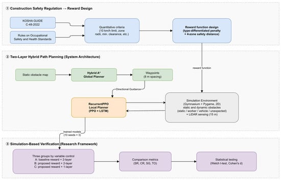
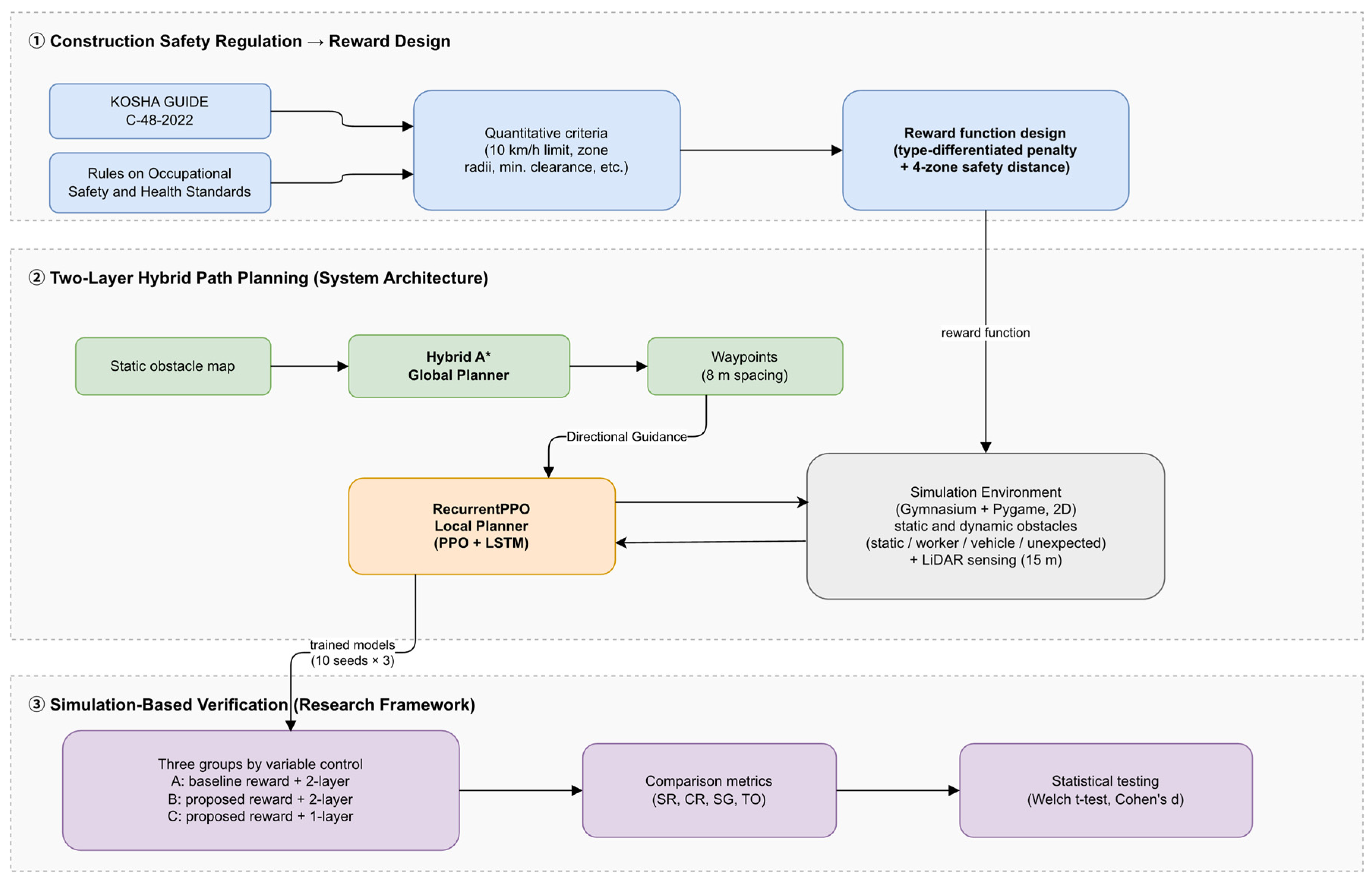
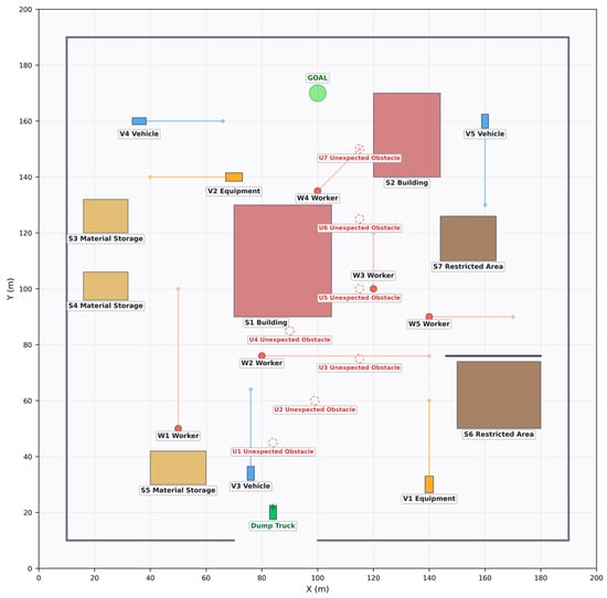
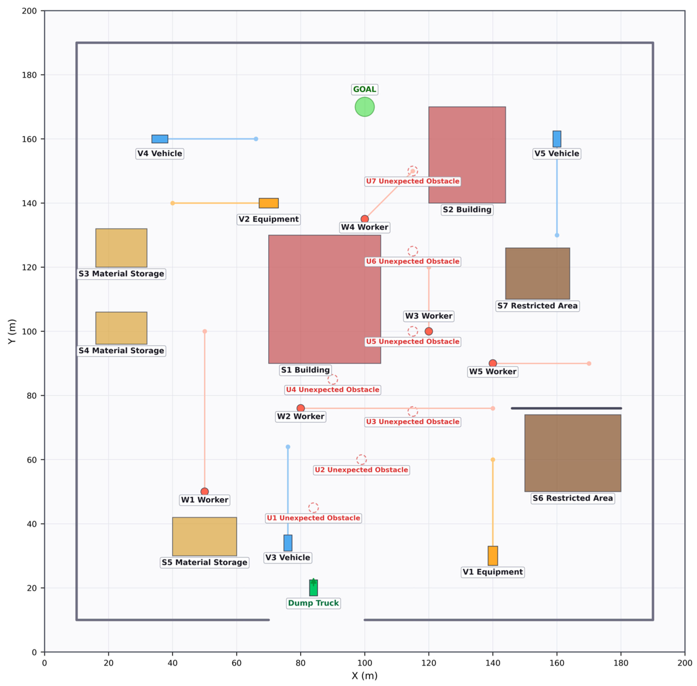
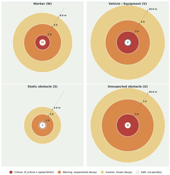
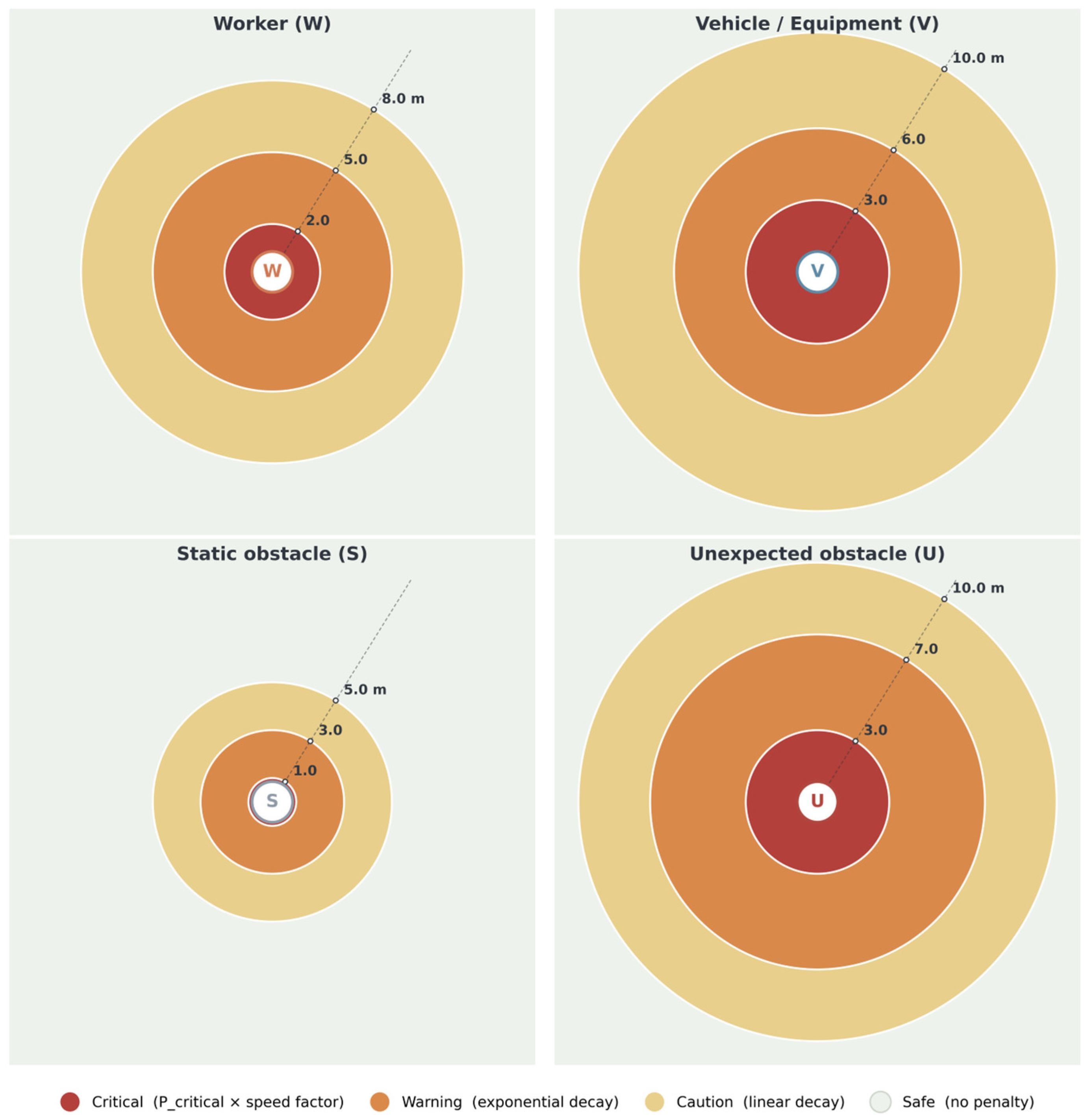
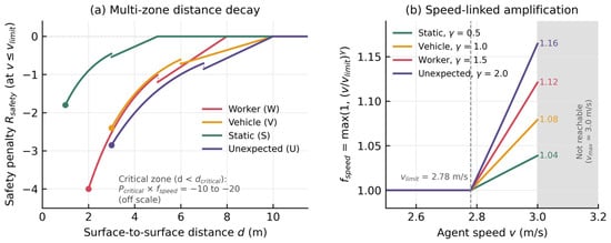
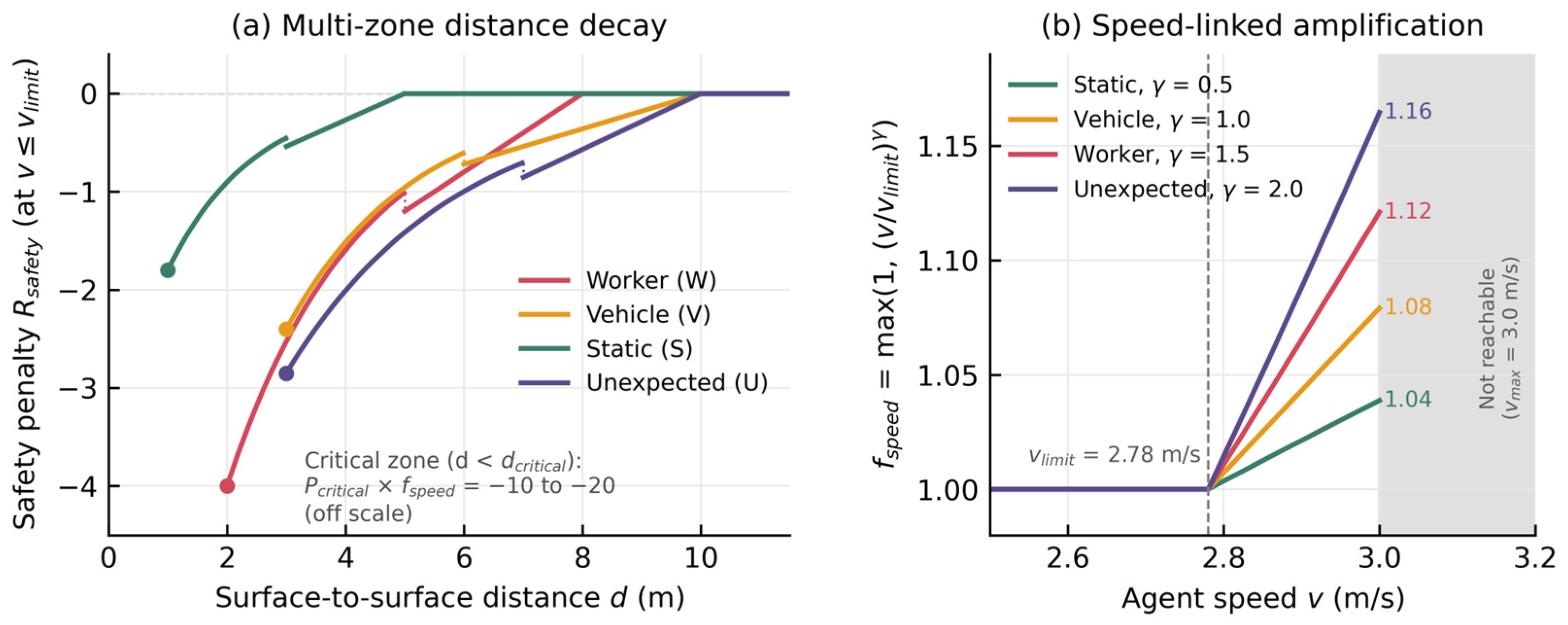
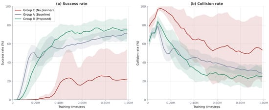
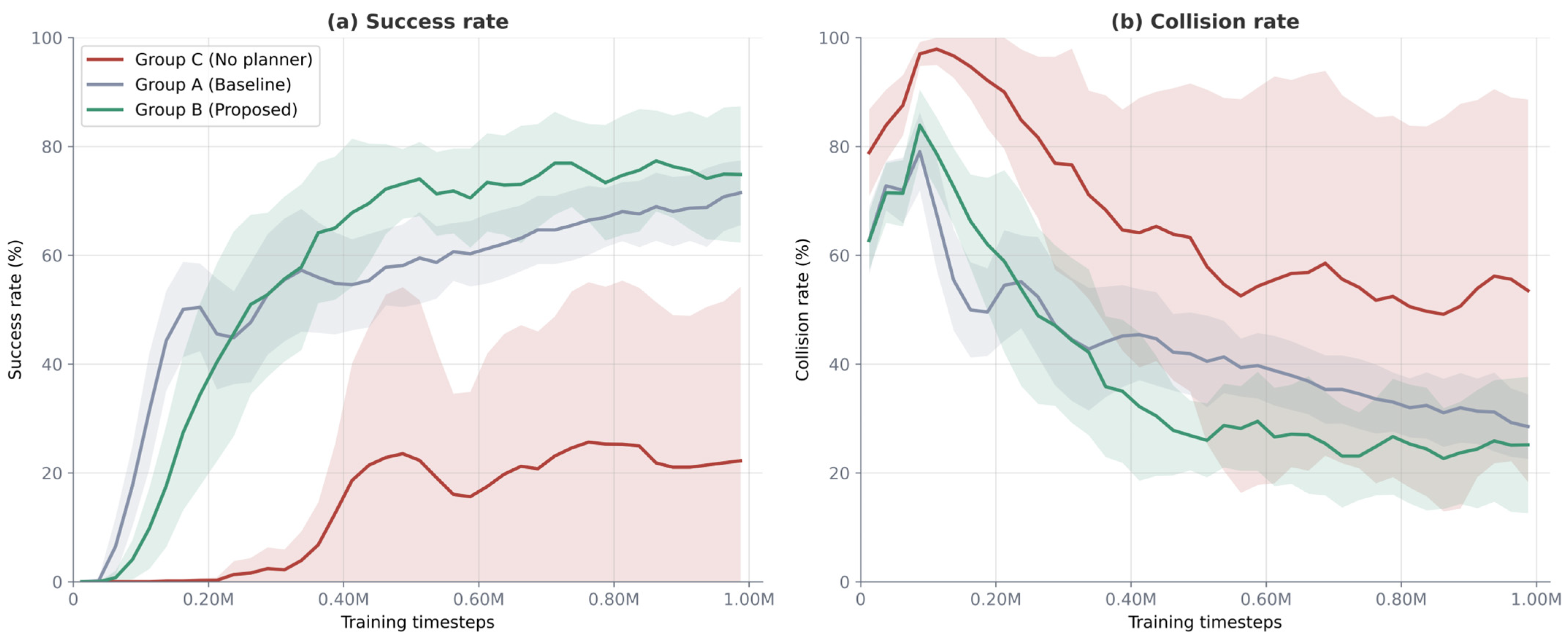
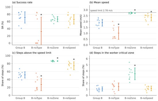
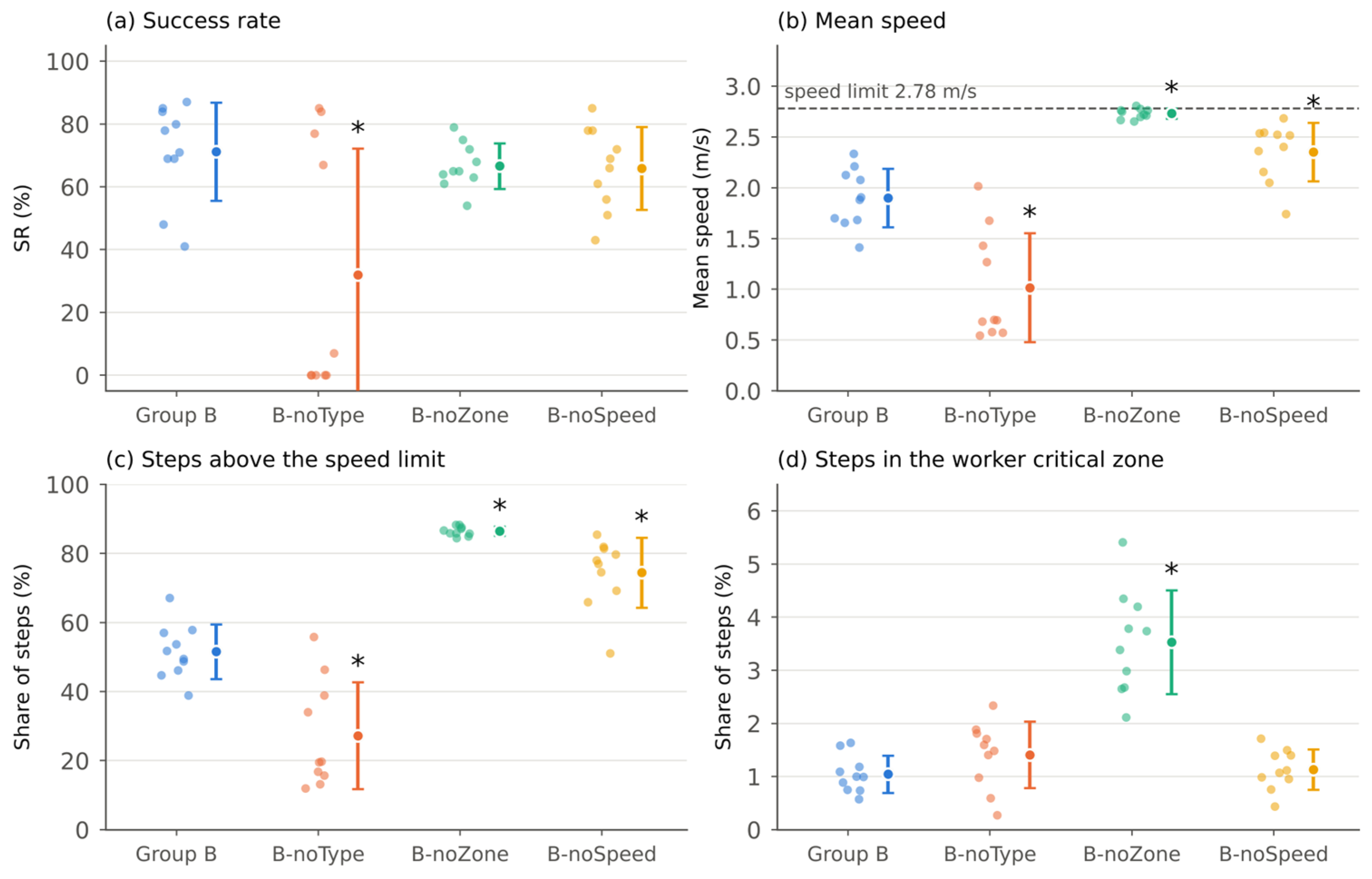
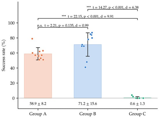

Disclaimer/Publisher’s Note: The statements, opinions and data contained in all publications are solely those of the individual author(s) and contributor(s) and not of MDPI and/or the editor(s). MDPI and/or the editor(s) disclaim responsibility for any injury to people or property resulting from any ideas, methods, instructions or products referred to in the content. |
© 2026 by the authors. Licensee MDPI, Basel, Switzerland. This article is an open access article distributed under the terms and conditions of the Creative Commons Attribution (CC BY) license.