


Abstract
Electrical resistivity provides a rapid, non-destructive indicator for condition assessment of cementitious construction materials, while its mechanical interpretation is governed by the active degradation mechanism. This study investigates an all-solid-waste red-mud cementitious material under Bayer-process leachate immersion, alkaline burial and freeze–thaw cycling using measured unconfined compressive strength (UCS) and 50-kHz bulk electrical resistivity as the experimental basis. Environment-specific calibration showed strong within-domain UCS-resistivity relationships (R2 = 0.912–0.971), with distinct calibration slopes among exposure conditions, supporting mechanism-aware interpretation. Experiment-constrained scenario states were then used to examine surrogate-model behavior, cross-domain transfer, electromechanical mismatch and uncertainty propagation. Environment conditioning markedly reduced ambiguity within the constructed scenario space, and leave-one-environment-out testing within the scenario database revealed clear domain shift, particularly for freeze–thaw exposure. Normalized mismatch descriptors and SEM observations further distinguished electrically leading chemical deterioration from mechanically leading freeze–thaw damage. The resulting framework integrates non-destructive electrical response, mechanical integrity and uncertainty at the material scale, providing an environment-aware framework for condition assessment of clinker-free, waste-derived cementitious materials. Experimental UCS–resistivity calibration was based on 20 measured exposure states; 14 additional coordinates and their bounded numerical realizations supported model comparison within the constructed scenario space. The reported surrogate-validation scores therefore characterize scenario-space model behavior rather than predictive accuracy on new experimental specimens.
1. Introduction
Bauxite residue (red mud) is produced in large quantities during alumina refining and remains challenging to reuse because of its high alkalinity, fine particle size and mineralogical complexity [1,2,3]. A promising route is to combine red mud with complementary industrial by-products to form low-clinker cementitious construction materials for backfilling, stabilization and related engineering applications. Their practical value, however, depends not only on initial strength but also on whether coupled mechanical and transport-related properties remain stable under chemically aggressive and freeze–thaw environments [4,5,6]. The RM–FA–SS–PG formulation investigated here differs from conventional externally alkali-activated geopolymer binders by exploiting the residual alkalinity of Bayer red mud together with aluminosilicate, calcium and sulfate sources, without adding a commercial alkali activator. Its prospective applications include non-load-bearing backfilling and stabilization, where durability under variable moisture, alkaline exposure and freezing conditions is central to material selection. Related binder studies provide a useful comparison for interpreting the material-specific durability mechanisms.
Electrical resistivity is attractive for such assessment because it is rapid, non-destructive and sensitive to pore-solution conductivity, connectivity of water-filled pathways and reaction progress [7,8,9,10]. Its mechanical meaning is nevertheless environment-dependent. Chemical exposure can promote dissolution–precipitation processes while freeze–thaw cycling acts mainly through phase change, hydraulic pressure and interface damage [11,12,13]. The same resistivity change may therefore correspond to different strength states, making a single universal resistivity–strength conversion difficult to justify.
Data-driven methods offer a practical way to address this ambiguity, provided that model complexity remains consistent with the size and structure of the available dataset. Linear regression retains transparent engineering meaning, whereas Gaussian-process regression (GPR), support-vector regression and tree-based methods can represent nonlinear behavior and, in the case of GPR, predictive uncertainty [14,15,16,17,18,19,20]. Recent studies on concrete, geopolymer and red-mud-based materials confirm the value of combining electrical indicators with machine learning for durability assessment, but they also show that transferability depends strongly on whether the training data span the relevant environmental domain [21,22,23,24,25,26,27,28,29,30,31,32,33,34,35,36,37,38].
Accordingly, the key challenge is not merely to reduce model error, but to construct an environment-conditioned interpretation framework that separates measured material performance from scenario-based model interrogation. In particular, resistivity should be treated as a monitoring signal whose structural meaning is jointly defined by exposure history and auxiliary state descriptors rather than as a standalone proxy for compressive strength [39,40].
Although previous studies have examined electrical resistivity and mechanical performance in cementitious materials, the interpretation of their relationship across different degradation environments remains an important challenge. For the RM–FA–SS–PG system investigated here, this study integrates environment-specific experimental calibration with numerical assessment of model transferability, electromechanical mismatch and uncertainty propagation. The resulting framework provides a mechanism-aware approach to interpreting electrical resistivity and supports more informative condition assessment of waste-derived cementitious materials.
The present study therefore focuses on three linked questions: whether the UCS-resistivity relation shifts systematically among degradation mechanisms; whether explicit environmental conditioning reduces ambiguity in small-data prediction; and whether divergence between normalized electrical and mechanical degradation can distinguish transport-sensitive change from loss of load-bearing continuity. The main contribution is an environment-conditioned condition-assessment framework that integrates measured calibration, domain-shift testing, electromechanical mismatch descriptors and uncertainty-aware screening. This combination extends conventional resistivity-strength analysis from a single empirical relationship toward a mechanism-aware assessment strategy in which measured observations support material-performance interpretation and experiment-constrained numerical states expand the analysis of model behavior and scenario sensitivity. The integrated workflow is summarized in Figure 1. In contrast to the previously established mixture-design approach [5] and the corrosive-salt/freeze–thaw lifetime analysis [6], this study examines environment-specific measured UCS–resistivity relations and separately uses experiment-constrained scenarios to assess transferability, mismatch and screening uncertainty. The distinction from a conventional environment-wise regression is the combined interpretation of normalized electrical–mechanical mismatch, cross-regime transfer diagnostics and threshold-dependent screening; these additional stages interrogate complementary aspects of the same measured and scenario-derived responses, not independent experimental datasets.
Figure 1.
Integrated experimental–numerical assessment framework.
2. Materials and Methods
2.1. Raw Materials and Mixture Design
The binder consisted of Bayer-process red mud (RM), fly ash (FA), steel slag (SS) and phosphogypsum (PG) at a fixed dry-mass ratio of 54:27:9:10. RM supplied residual alkalinity and Fe-Al-bearing phases; FA provided a Si-Al-rich glassy fraction; SS supplied Ca-rich reactive components; and PG provided Ca and sulfate. The same formulation has previously shown the ability to form a mechanically competent matrix without Portland cement or an added commercial alkali activator [5]. The selected oxide compositions are summarized in Table 1. Table 1 lists the principal reported oxides; the listed percentages do not constitute a complete chemical analysis. The chosen proportions were retained throughout the three exposure programs, so differences in the observed trajectories can be discussed without introducing mixture composition as a variable. The roles assigned to RM, FA, SS and PG reflect their reported oxide compositions and the previously established formulation [5], rather than a new mixture-optimization experiment.
Table 1.
Selected oxide composition of the raw materials (wt.%).
2.2. Specimen Preparation and Environmental Exposure
All solid constituents were first air-dried in the laboratory until their masses were stable, manually disaggregated, and passed through a 2 mm sieve. RM, FA, SS and PG were weighed at a dry-mass ratio of 54:27:9:10 and dry-mixed mechanically for 5 min until a visually homogeneous blend was obtained without obvious powder segregation or agglomeration. The dry-blended constituents were then combined with mixing liquid at the recorded solid-to-liquid ratio (S/L) of 0.3 and placed in cylindrical steel molds with a nominal diameter of 50 mm and height of 50 mm. Specimens were formed by static pressing with a hydraulic device. After forming, specimens were allowed to stabilize before demoulding and were then transferred to a controlled curing environment at 20 ± 1 °C and approximately 98% relative humidity until the designated pre-exposure age for each program. The same preparation and curing route was applied to all specimens used for mechanical, electrical and environmental-exposure comparisons.
The recorded solid-to-liquid ratio (S/L) of 0.3 describes the proportion of solid constituents to the mixing liquid. The powder constituents were therefore dry-mixed before liquid incorporation and static pressing. Subsequent curing at 20 ± 1 °C and approximately 98% relative humidity was intended to restrict moisture loss and provide favorable conditions for continued binder reactions.
The static-forming protocol was standardized by increasing axial pressure at 0.5 MPa s−1 to a nominal forming pressure of 10 MPa, maintaining the peak pressure for 60 s, and then unloading gradually. For the 50 mm-diameter mould, this pressure corresponds to a peak forming load of approximately 19.6 kN. Because the specimens were pressure-formed rather than impact-compacted, preparation consistency was controlled by the pressure–time history rather than by an impact compaction energy. Three independently prepared specimens were assigned to each exposure state (n = 3), providing a common replicate structure for the mechanical and electrical comparisons. The nominal cylinder volume is 98.17 cm3, and the loaded area is 1963.50 mm2.
Three environmental programs were imposed. For leachate immersion, cured specimens were fully submerged in authentic Bayer-process red-mud leachate, with the liquid surface maintained above the specimen top and without chemical adjustment of the original leachate. For alkaline burial, specimens were completely embedded in original red mud so that they remained in contact with the native alkaline pore liquid and fine solid phase; the moisture state and chemical composition of the red mud were not artificially adjusted. Chemical exposure states were evaluated at 0, 7, 14, 28, 60, 90 and 180 d. For freeze–thaw exposure, specimens with dry surfaces were frozen at −20 °C for 12 h and subsequently thawed at 25 °C for 12 h; one freeze–thaw cycle therefore lasted 24 h, and measurements were obtained after 0, 2, 4, 6, 8 and 10 cycles. The exposure programs are evaluated separately, with pore-liquid chemistry and moisture conditions considered when interpreting electrical changes. Leachate immersion provided continuous contact with the original Bayer-process liquid, whereas alkaline burial involved contact with both native red-mud solids and their associated pore liquid. The exposure media were used without artificial adjustment of their chemical composition. The available exposure record identifies medium provenance and contact conditions, but does not contain measured pH or electrical conductivity of the exposure media or specimen saturation at the measurement states. These properties are therefore considered when interpreting resistivity rather than assigned unmeasured numerical values. Differences between the two series should therefore be interpreted as program-level responses, not as the isolated effect of alkalinity alone.
The three exposure programs were initiated from different pre-exposure states and were therefore analyzed within program rather than pooled as exchangeable replicates. Chemical exposure was characterized by a mid-term increase in strength and resistivity followed by late deterioration, whereas the freeze–thaw series exhibited predominantly monotonic degradation. These measured states constitute the experimental backbone; the experiment-constrained scenario extensions used for model interrogation are defined in Section 2.5. Age-matched neutral-immersion and standard-curing reference trends are also reported in the associated dissertation [41]. The non-aggressive reference curves in [41] provide an important comparison for the continuing reaction of the binder. Their qualitative role is to distinguish strength development during exposure from a claim that all early strength gain was caused by chemical attack; a treatment-specific increment requires matched numerical differences at the same age.
2.3. Mechanical and Electrical Testing
UCS was measured on statically pressed Φ50 mm × 50 mm cylinders using an electro-hydraulic servo universal testing machine under monotonic axial compression. Before loading, specimen surfaces were kept dry, and samples showing visible edge loss, cracking or unacceptable dimensional deviation were excluded. Axial displacement was applied at 1.0 mm min−1, corresponding to a nominal axial strain rate of 2.0% min−1 for the 50 mm-high specimens, until global failure. The maximum axial load Pmax was used to calculate the unconfined compressive strength qu from the original loaded area A0. Three independent specimens were tested at each state, and the arithmetic mean was used as the representative UCS for subsequent environment-specific calibration and trajectory analysis. The constant 1:1 cylinder aspect ratio enables comparisons within this study, but platen restraint may affect absolute UCS values relative to those obtained using more slender specimens.
qu = Pmax/A0
ρ = RA/L
Electrical resistance was measured using an LCR digital bridge operated with an alternating signal at 50 kHz to reduce low-frequency electrode-polarization effects. The upper and lower specimen faces were cleaned before testing to ensure stable electrode contact, and measurements were conducted at laboratory temperature (20 ± 2 °C). After a 30 s contact-stabilization period, three consecutive resistance readings were recorded for each specimen and averaged. Bulk resistivity ρ was calculated from measured resistance R, cross-sectional area A and specimen height L using the original specimen geometry. The state-level resistivity was then obtained as the mean of three independently prepared specimens (n = 3). Bulk electrical resistivity reflects the combined influences of pore-fluid conductivity, moisture-dependent ionic conduction and the connectivity of conductive pathways within the cementitious matrix. Consequently, changes in resistivity under different exposure conditions are interpreted alongside the corresponding UCS results, considering both the evolution of the solid matrix and the electrical contribution of the pore fluid. Pore-fluid composition and specimen saturation were not quantified at each electrical measurement; hence, comparisons between exposure programs consider both the solid matrix and its conductive pore liquid. For this nominal geometry, the unit-consistent conversion is ρ (Ω·m) = 0.039270 R (Ω), provided that R denotes the bulk-resistance component of the measured impedance. This geometric conversion is independent of environmental exposure, whereas the measured resistance can vary with pore-solution ion concentration, saturation and electrode contact. Thus, the resulting resistivity is evaluated alongside UCS rather than converted directly into a pore-size or crack-density measurement.
Three independently prepared specimens were tested at each exposure state, and their mean UCS and electrical resistivity values were retained for subsequent analysis. Individual specimen-level measurements were not separately archived after aggregation, so experimental standard deviations and replicate-level confidence intervals cannot be reconstructed. The environment-specific calibration describes relationships among measured state means, rather than the precision of individual-specimen measurements.
2.4. Environment-Specific Electromechanical Calibration
For each exposure program, the relationship between resistivity and UCS was expressed as
where U is UCS, a is the intercept, and b is the environment-specific calibration slope. The experimental fits were evaluated using b and R2. Differences among programs were used to quantify the sensitivity of electrical response to mechanical state under distinct boundary conditions. The fitted calibration coefficients are summarized in Table 2. Equation (3) is an empirical linear calibration using the reported measured state means (seven exposure states for each chemical program and six for freeze–thaw); the coefficients in Table 2 are fitted descriptors, not independently derived material constants. The reported R2 values quantify goodness of fit among measured exposure-state means; they are not estimates of within-state specimen dispersion, replicate-level measurement uncertainty or confidence intervals. The units are U (MPa), a (Ω·m) and b (Ω·m MPa−1). The coefficients allow a direct comparison of the observed electrical response per unit UCS across programs: the reported b values are 0.37, 0.55 and 0.50 Ω·m MPa−1 for leachate immersion, alkaline burial and freeze–thaw, respectively. These differences capture program-specific calibration behavior, although their physical interpretation must also consider changes in conductive pore fluid and saturation.
ρ = a + bU
Table 2.
Environment-specific experimental UCS-resistivity calibration.
2.5. Experiment-Constrained Numerical Scenario Augmentation
The measured program provides discrete but representative anchor states along three distinct degradation paths. To obtain a denser description of the response between and beyond these anchors, a constrained numerical scenario procedure was introduced. Measured initial, turning and late states were used as physical anchors, and intermediate or extended states were generated so that each trajectory preserved the observed direction, turning point and relative deterioration pattern. The chemical series were extended to 120, 150, 210, 270 and 360 d, while the freeze–thaw series was extended to 15, 20, 30 and 40 cycles. These ages and cycle counts define experiment-constrained scenario coordinates for interpolation, sensitivity analysis and trajectory comparison.
Scenario construction used 20 experimental anchor states and the 14 additional age or cycle coordinates defined in Table 3. The means at the additional coordinates were prescribed to follow the observed trajectory directions and turning points; they are numerical scenario inputs, not results of additional material tests. Five bounded realizations were then used for each of the 34 coordinates. The documented procedure specifies the state coordinates and perturbation magnitudes, but does not supply the complete state-by-variable mean matrix, the individual realized perturbations or their exact sampling rule. Record-level reconstruction of all 170 numerical records would require those original numerical files.
Table 3.
State matrix used in the experimental–numerical database.
For each scenario state, five bounded realizations were generated around its prescribed mean to provide a controlled sensitivity envelope. Relative perturbation magnitudes of 3.5% for UCS, 2.5% for resistivity, 1.2% for ultrasonic pulse velocity and 1.8% for water absorption were specified, together with small absolute perturbations for mass change and extract pH. These reported magnitudes describe the prescribed numerical variation rather than experimentally measured replicate dispersion. Across 34 coordinates, the resulting 170 scenario records were used to compare surrogate models and examine sensitivity, while the environment-specific calibrations in Table 2 remained based solely on measured state means. The assigned scenario covariates are modeling inputs, not independently tested additional specimens.
2.6. Normalized Degradation Descriptors
To compare mechanical and electrical deterioration on a common scale, the maximum-strength/resistivity state within each program was used as the reference for chemical exposure, whereas the initial state was used for freeze–thaw. The normalized descriptors were
where increasing D indicates increasing deterioration. The difference Dρ-DU provides a simple measure of electromechanical desynchronization.
DU = 1 − U/Uref, Dρ = 1 − ρ/ρref
2.7. Machine-Learning Models and Grouped Validation
UCS was used as the prediction target. The core predictor set contained electrical resistivity, normalized exposure intensity and exposure category. A second extended predictor set additionally included ultrasonic pulse velocity, mass change, water absorption and extract pH. Four model classes were examined: linear regression, SVR with a radial-basis kernel, random forest and GPR. The GPR covariance function combined a constant kernel, radial-basis kernel and white-noise term. Auxiliary values assigned to generated states are modeling covariates, not additional independent experimental measurements. The extract-pH covariate assigned to generated scenarios should not be interpreted as a direct measurement of leachate or burial-medium pH.
Model evaluation used five-fold GroupKFold splitting, with all five numerical realizations belonging to a given exposure state assigned to the same validation fold. The scenario-space performance metrics were R2, root-mean-square error (RMSE) and mean absolute error (MAE). Grouping prevents realizations of a single state from being divided between training and validation, although different scenario-state means may share the same experimental anchors. Accordingly, the scores describe model behavior across held-out groups within the constructed scenario space. Leave-one-environment-out tests provide a complementary comparison of transfer between the three represented exposure regimes within this same numerical database.
2.8. Weibull-Type Freeze–Thaw Degradation Model
The extended freeze–thaw mean scenario trajectory was described using a two-parameter Weibull-type degradation function
where N is the number of freeze–thaw cycles, m is the shape parameter, and η is the scale parameter. The fitted curve summarizes the constructed trajectory and identifies scenario cycle counts associated with retained-strength ratios of 0.60, 0.50 and 0.40. Values inferred beyond the measured 10-cycle range are extrapolative descriptors of the experiment-constrained scenario. In particular, a threshold crossing on the fitted curve is an estimated scenario coordinate, not an observed specimen-failure event. The Weibull shape and scale parameters are used to describe the constructed deterioration path, rather than to infer a population lifetime distribution from independently observed failures.
DU(N) = 1 − exp[−(N/η)m]
2.9. Monte Carlo-Based Probability Estimation
Prediction uncertainty was propagated into a state-level screening probability. A lower-strength boundary equal to 60% of the maximum UCS within each exposure program was adopted as a normalized reference boundary for comparative assessment. The total prediction standard deviation combined the grouped-CV RMSE of the extended-feature GPR model with a nominal 5% resistivity-measurement uncertainty converted to strength through the environment-specific calibration slope. The 5% value provides a transparent engineering scenario for demonstrating uncertainty propagation, while the influence of the selected strength boundary was examined through sensitivity analysis. For each state, the conditional probability of falling below the adopted strength boundary, denoted Pf, was calculated as
Pf = P(U < Ulim), R = 1 − Pf
The complementary quantity R = 1 − Pf is used as a screening probability that integrates the selected performance boundary with model and measurement uncertainty. It supports state comparison, monitoring prioritization and identification of narrowing performance margins. To quantify boundary sensitivity, representative late states were recalculated using 50%, 60% and 70% of program-maximum UCS as alternative limits. As a reproducibility check of the conditional Gaussian screening calculation, 10,000 pseudo-random samples were drawn for each of the 13 representative states using seed 42. The same draws were evaluated against limits of 50%, 60% and 70% of the program-peak UCS; these are scenario samples and do not represent additional material measurements or independently calibrated uncertainty. The 60% boundary is an illustrative, material-normalized screening convention rather than a code-based serviceability or failure criterion. The 50%, 60% and 70% thresholds use the same underlying state means and uncertainty assumptions, allowing the influence of the decision boundary to be isolated from changes in model fitting. As the boundary increases, the conditional probability of falling below it cannot decrease for a fixed predictive distribution. This monotonicity provides an additional check on the numerical screening results and makes the threshold choice visible to engineering interpretation.
2.10. Feature Ablation and Cross-Environment Transferability
The contribution of environmental conditioning to state discrimination was quantified by feature ablation. Four GPR configurations were compared under the same state-grouped protocol: resistivity only; resistivity plus normalized exposure intensity; resistivity, exposure intensity and environment category; and an extended-feature model additionally containing ultrasonic pulse velocity, mass change, water absorption and pH. Changes in held-out R2 and RMSE were used to assess whether the added variables reduced ambiguity within the represented scenario space; because environment category is a domain label, the improvement after its inclusion is interpreted as evidence of domain dependence rather than a direct mechanistic effect of the categorical variable itself.
Cross-environment transfer was examined through leave-one-environment-out testing. Models were fitted on two exposure programs and evaluated on the third within the preconstructed scenario dataset. This test directly examines whether a mapping learned in one pair of degradation domains can be transferred to a mechanistically different third domain. Across the three representative exposure families, the results provide a physically interpretable measure of domain shift and clarify when environment-specific calibration adds the greatest value. The scenario matrix was assembled before environment withholding, so the results describe transfer sensitivity within the represented domains. A negative transfer score on a withheld environment is therefore evidence of model mismatch across the three represented degradation regimes, not an estimate of predictive error on an independently collected new specimen population. In this sense, domain withholding identifies where an electrical–strength mapping requires recalibration rather than proving external generalization.
2.11. Electromechanical Mismatch Descriptors
To distinguish electrical-leading and mechanical-leading deterioration, an electromechanical mismatch index M and a coupling ratio Cem were defined as M = |Dρ − DU| and Cem = Dρ/DU. The ratio was evaluated only for states with DU > 0.03 to avoid numerical instability as the denominator approaches zero; this cutoff is used consistently as a plotting convention. M quantifies the magnitude of desynchronization, whereas Cem identifies its direction: Cem > 1 denotes a greater relative electrical change, Cem ≈ 1 indicates coupled deterioration, and Cem < 1 denotes a greater relative mechanical change. These descriptors are used as comparative diagnostic state variables.
2.12. Dimensionless State-Space Construction
A dimensionless integrity-state representation was introduced to separate trajectory geometry from absolute scale. Mechanical and electrical integrity were defined as IU = U/Uref and Iρ = ρ/ρref, respectively. Each environmental state was therefore represented in the plane I = (Iρ, IU). The 1:1 line denotes synchronous electromechanical degradation; states above the line retain a larger fraction of mechanical integrity than electrical integrity, while states below the line indicate stronger relative mechanical deterioration.
IU = U/Uref, Iρ = ρ/ρref
2.13. Monitoring-Priority State Metric
Electromechanical mismatch and screening probability were combined to provide a monitoring-priority map without collapsing them into a single scalar score. The mismatch M quantifies disagreement between electrical and mechanical deterioration, while R quantifies the conditional screening margin relative to the adopted normalized performance boundary. Four descriptive state regions were considered: low mismatch–high R, high mismatch–high R, low mismatch–low R and high mismatch–low R. The map provides a structured basis for prioritizing verification among the represented states.
2.14. Uncertainty Decomposition
The total uncertainty associated with resistivity-assisted UCS estimation was decomposed into a model component and an electrical-measurement component. The model component was represented by the grouped-CV RMSE of the extended-feature GPR model. The measurement component was propagated through the environment-specific linear calibration. Assuming independent contributions, the total standard deviation was evaluated as
σtot = (σmodel2 + σmeas2)1/2
This decomposition makes it possible to distinguish whether additional experimental effort should be directed toward improving the prediction model or toward reducing measurement variability. Because the electrical-measurement component decreases as the calibration slope increases, the same nominal resistivity error can translate into substantially different UCS uncertainty in different exposure domains. The grouped-CV RMSE is used here as a scenario-based model-error scale rather than an independently calibrated predictive standard deviation.
The uncertainty assessment combines the grouped-validation RMSE with an assumed 5% electrical-resistivity measurement uncertainty propagated through the environment-specific calibration relationship. The resulting uncertainty estimates are incorporated into the Monte Carlo screening analysis to examine the sensitivity of material-performance assessment to different strength thresholds. This approach enables quantitative comparison of screening margins among exposure states and provides useful information for identifying conditions requiring closer monitoring.
2.15. Additional Probabilistic and Gaussian-Process Formulation
For cross-program comparison, exposure was represented by a dimensionless coordinate ξe. For the two chemical programs, x denotes exposure age, whereas for freeze–thaw x denotes cycle number. This normalization removes the dimensional mismatch between days and cycles while preserving within-program ordering:
ξe = x/xmax
The GPR model was formulated with a squared-exponential covariance term and an additive white-noise component. For predictor vectors x and x′, the covariance was written as
k(x,x′) = σf2 exp[−||x − x′||2/(2ℓ2)] + σn2δ(x,x′)
Given training inputs X, target vector y and a new state x*, the posterior predictive mean and variance were evaluated from the standard Gaussian-process expressions
μ* = k*T(K + σn2I)−1y
σ*2 = k(x*,x*) − k*T(K + σn2I)−1k*
For Equations (11) and (12), K, k* and k(x*,x*) denote covariance quantities from the noise-free squared-exponential component of Equation (10); the observation-noise term σn2I is added only once, and the predictive variance refers to the latent response rather than an additional noisy observation.
These expressions make the uncertainty output mechanistically useful rather than decorative: a state can be located not only by its predicted UCS but also by the width of the admissible prediction region. Under an approximate Gaussian error representation, the distance from a lower performance boundary can additionally be expressed as a standardized margin z:
z = (μU − Ulim)/σtot, R ≈ Φ(z)
The analytical margin in Equation (13) was used only as an interpretive check on the Monte Carlo screening calculation; the reported screening probabilities remain conditional on the adopted performance boundary and uncertainty assumptions.
2.16. Cross-Scale Microstructural Corroboration
Microstructural observations from the same material system were used to test whether the electromechanical trajectories were consistent with independently observed structural evolution. SEM subsamples were taken from the specimen interior and trimmed to approximately 10 mm × 10 mm × 3 mm, dried at 60 °C, mounted and gold-coated before observation. These images were not used as machine-learning predictors; they provide an independent qualitative check on the proposed transition from reaction-assisted densification to dissolution/cracking-controlled deterioration.
3. Results
3.1. Experimental Backbone and Numerical Scenario Trajectories
In the measured leachate-immersion series, UCS increased from 9.25 MPa initially to 35.86 MPa at 90 d and then decreased to 31.86 MPa at 180 d. Resistivity increased from 2.48 to 12.56 Ω·m before declining to 9.33 Ω·m. The numerical scenario preserves this experimentally observed reversal and extends the post-peak path to UCS values of 29.9, 26.2 and 22.0 MPa at 210, 270 and 360 d, respectively, with corresponding resistivity values of 8.4, 7.1 and 6.0 Ω·m. Values beyond 180 d are scenario states, not measurements.
In the measured alkaline-burial series, UCS increased from 9.21 MPa initially to 15.28 MPa at 7 d, decreased to 10.70 MPa at 14 d and reached 29.72 MPa at 90 d. The measured late state was 24.37 MPa at 180 d, with resistivity decreasing from a 90 d value of 13.35 Ω·m to 10.47 Ω·m. The scenario trajectory subsequently extends to UCS values of 18.7 and 15.5 MPa and resistivities of 7.4 and 5.5 Ω·m at 270 and 360 d, respectively. The age-matched reference trends reported in [41] indicate that strength development also occurs under non-aggressive conditions. Therefore, the initial strength increases observed during leachate immersion and alkaline burial are interpreted as the overall responses of the exposed specimens, rather than being attributed solely to the chemical exposure.
Freeze–thaw produced near-direct degradation over the measured range: UCS decreased from 18.45 MPa initially to 9.60 MPa after 10 cycles, while resistivity decreased from 12.28 to 7.50 Ω·m. The numerical scenario extends this path to 15, 20, 30 and 40 cycles with UCS values of 7.20, 5.40, 3.20 and 2.00 MPa and resistivities of 6.30, 5.40, 4.20 and 3.50 Ω·m, respectively. The monotonic extension is therefore a model-testing construct beyond the experimentally observed 0–10 cycle range. The corresponding UCS and resistivity trajectories are shown in Figure 2 and Figure 3, respectively. In Figure 2 and Figure 3, open symbols distinguish the numerically extended states from the filled markers used for the measured environmental states; the source-level classifications and exposure coordinates are listed in Table 3.
Figure 2.
UCS trajectories across measured and extended environmental states.
Figure 3.
Electrical-resistivity trajectories across measured and extended states.
3.2. Environment-Dependent Electromechanical Calibration
The three experimental programs all show positive coupling between UCS and resistivity, but the fitted coefficients differ substantially. The slope is 0.37 Ω·m MPa−1 for leachate immersion, 0.50 Ω·m MPa−1 for freeze–thaw and 0.55 Ω·m MPa−1 for alkaline burial. The corresponding R2 values are 0.925, 0.912 and 0.971. These differences indicate that the electrical response per unit mechanical change is exposure dependent. The fitted slopes describe different electrical sensitivities per unit strength change, not statistically established differences in a universal material constant; pore-solution conductivity and the extent of mechanically effective particle bonding provide complementary physical interpretations.
The lower slope under leachate immersion is consistent with the influence of an ion-bearing pore liquid, which partially offsets the resistivity increase associated with matrix densification. Alkaline burial exhibits the largest slope and highest R2, indicating closer state-to-state correspondence between load-bearing development and restriction of conductive pathways. Freeze–thaw produces an intermediate slope and a nearly monotonic trajectory. The slope differences quantify the environment-dependent electrical sensitivity of the same nominal mechanical change: a given increase or loss in UCS corresponds to a smaller resistivity response in leachate than in alkaline burial. This explains why a single conversion equation would introduce systematic bias across exposure domains. The fitted relationships are summarized in Figure 4. The fitted slopes provide descriptive comparisons across the six or seven measured state means in each program.
Figure 4.
Environment-specific UCS–resistivity calibration.
3.3. Scenario-Space Machine-Learning Performance
Grouped cross-validation within the constructed scenario space shows that surrogate-model performance depends more strongly on predictor information than on algorithmic complexity. Using resistivity, normalized exposure intensity and exposure category, linear regression gives R2 = 0.946, RMSE = 2.22 MPa and MAE = 1.65 MPa. SVR gives R2 = 0.958, whereas random forest gives R2 = 0.942. Core-feature GPR reaches R2 = 0.977 and RMSE = 1.46 MPa. The relatively narrow spread among linear regression, SVR and GPR indicates that the represented problem is not intrinsically high-dimensional once the exposure domain is identified; rather, the principal challenge is resolving the appropriate response manifold. This favors parsimonious models when calibration data are limited.
Adding ultrasonic pulse velocity, mass change, water absorption and pH gives the lowest internal grouped-validation error in the augmented state space. The extended-feature GPR yields R2 = 0.986, RMSE = 1.15 MPa and MAE = 0.85 MPa. The improvement over core-feature GPR is modest, indicating that resistivity and exposure history encode most of the information represented in the constructed state space, while auxiliary variables mainly reduce local ambiguity near turning states. These metrics characterize internal grouped-validation performance within the augmented scenario space. The model metrics are summarized in Table 4, with the model comparison and extended-feature GPR results shown in Figure 5 and Figure 6, respectively.
Table 4.
Scenario-space grouped-validation performance of the tested UCS models.
Figure 5.
Scenario-space grouped-CV R2 of the tested UCS models.
Figure 6.
Grouped-CV performance of the extended-feature GPR within the augmented state space.
3.4. Freeze–Thaw Degradation Model
The Weibull-type model closely represents the constructed freeze–thaw scenario trajectory, with m = 0.923, η = 15.99 cycles and R2 = 0.993. The fit summarizes the combined measured and extended scenario path, including states beyond the measured 10-cycle range. The fitted shape parameter below unity describes rapid early damage followed by smaller incremental change at higher cycle counts within this scenario representation. The fit and post-10-cycle thresholds describe the combined measured–scenario trajectory. The 15–40-cycle segment represents extrapolation from the six measured freeze–thaw states between 0 and 10 cycles; its high fitted R2 assesses agreement with the prescribed trajectory, not experimental verification of deterioration beyond 10 cycles.
Within this scenario, retained-strength ratios of 0.60, 0.50 and 0.40 occur at approximately 7.7, 10.7 and 14.5 cycles, respectively. The first value lies within the measured cycle range, whereas the latter two are partly or wholly extrapolative and identify high-value ranges for subsequent experimental verification. The fitted degradation curve is shown in Figure 7.
Figure 7.
Weibull-type freeze–thaw degradation curve.
3.5. Probabilistic Screening Results and Sensitivity Analysis
The screening-probability calculation separates states that have similar mean trajectories but different uncertainty margins. For the chemical programs, R remains high near the 90 d optimum and decreases as the late-stage mean strength approaches the illustrative 60%-of-peak boundary. Under leachate immersion, the scenario mean remains above this boundary through 360 d, but the margin narrows at the final state because model and electrical-measurement uncertainty are no longer small relative to the remaining strength margin.
Alkaline burial reaches the illustrative boundary earlier because the late-stage decline is steeper. Freeze–thaw shows the fastest loss of screening margin: the probability of remaining above the 60%-of-peak boundary falls sharply around the measured-to-extended transition. As expected, the numerical value depends on the selected boundary. At L360, R changes from approximately 0.998 to 0.634 and 0.014 when the boundary is set to 50%, 60% and 70% of peak UCS, respectively; at A270 the corresponding values are 0.998, 0.743 and 0.057, and at F10 they are 0.607, 0.142 and 0.008. The sensitivity of R to the adopted boundary is therefore explicit. Representative screening probabilities are listed in Table 5, and their trajectory evolution is shown in Figure 8. Across the 39 state–threshold comparisons, the largest absolute difference between the 10,000-draw proportions and the Gaussian tail probabilities was 0.0095, consistent with finite sampling variability.
Table 5.
Representative Monte Carlo screening probabilities under the 60%-of-peak boundary.
Figure 8.
Screening probability along normalized exposure trajectories.
3.6. Feature Ablation and Environment-Conditioned Learning
Feature ablation shows that a domain label is necessary to recover the distinct electrical–mechanical mappings represented in the scenario database. GPR using resistivity alone gives R2 = 0.295 and RMSE = 8.04 MPa under state-grouped validation. Adding normalized exposure intensity gives only a modest improvement (R2 = 0.341; RMSE = 7.78 MPa). Once the environment category is introduced, R2 rises to 0.977, and RMSE falls to 1.46 MPa; the extended-feature configuration gives R2 = 0.986 and RMSE = 1.15 MPa. The abrupt gain indicates that the three exposure programs occupy different response domains, while the environment label compactly represents domain information already embedded in the augmented trajectories. The ablation results are summarized in Table 6 and Figure 9.
Table 6.
Feature-ablation results for GPR-based UCS prediction.
Figure 9.
Effect of feature conditioning on GPR performance.
3.7. Cross-Environment Transferability and Domain Shift
Leave-one-environment-out testing provides a stricter diagnostic of domain shift than within-domain grouped validation. Linear regression trained on the other two environments gives RMSE values of 10.41 MPa for leachate immersion, 5.29 MPa for alkaline burial and 12.19 MPa for freeze–thaw. GPR reduces the leachate error to 7.28 MPa but does not eliminate the shift; when freeze–thaw is withheld from training, the GPR RMSE reaches 14.67 MPa. Negative R2 values for several held-out programs indicate that a mapping learned from the remaining domains is inadequate for the omitted mechanism. With only three environments, however, these values should be read as a stress test of incompatibility among the present domains rather than as a statistical estimate of general field transferability.
This result changes the interpretation of the machine-learning stage. The environment variable is useful because it partitions observations into distinct response domains; it should not be regarded as a substitute for measured physical variables such as saturation, temperature or pore-fluid conductivity. The failure of cross-domain transfer is consistent with different electrical–mechanical manifolds under chemical reaction and phase-change damage. Field-oriented application would therefore require environment-specific calibration or an independently validated regime-identification step before UCS estimation. The leave-one-environment-out metrics are summarized in Table 7 and Figure 10.
Table 7.
Leave-one-environment-out transferability of environment-agnostic models.
Figure 10.
Leave-one-environment-out transfer performance.
3.8. Feature Contribution and Extended-State Interpretation
Permutation analysis of the extended-feature GPR identifies ultrasonic pulse velocity as the variable associated with the largest loss of model performance when permuted, followed by environment category and electrical resistivity. Exposure intensity and water absorption contribute smaller incremental information, while pH and mass change add little within the present model. Because these predictors co-vary strongly with degradation state and some are numerically augmented, the permutation values are interpreted only as model sensitivity within this dataset; they are neither causal effects nor a stable ranking expected to transfer to other mixtures or environments.
The ranking is nevertheless physically coherent. Ultrasonic velocity responds directly to stiffness and crack development; environment category distinguishes reaction-controlled and phase-change-controlled regimes; and resistivity tracks the continuity of conductive liquid pathways. Their combination therefore spans complementary mechanical, environmental and transport-sensitive information. The resulting feature-contribution ranking is shown in Figure 11.
Figure 11.
Permutation-based feature contribution of the extended-feature GPR.
3.9. Electromechanical Mismatch and Degradation Regimes
The mismatch index separates three response regimes, with the evidence level determined by whether a state is measured or scenario-derived. At the measured 180 d leachate state, Cem is 2.31, indicating that normalized electrical deterioration exceeds normalized mechanical deterioration. Scenario states at 150 and 210–270 d retain the same electrical-leading tendency. Alkaline burial remains closer to synchronous behavior, whereas freeze–thaw shows mechanically leading degradation, with Cem near 0.80 over the later scenario range. The descriptors therefore summarize the direction of decoupling across the represented trajectories.
These regime differences provide a compact diagnostic interpretation. Cem > 1 indicates that transport-sensitive electrical response is changing faster than load-bearing capacity, which is consistent with localized pathway reopening under prolonged chemical exposure. Cem < 1 indicates mechanically dominant deterioration, as observed under distributed freeze–thaw damage. The mismatch variable therefore captures mechanism-sensitive information that is lost when UCS and resistivity are considered only through correlation. The three mismatch trajectories are compared in Figure 12.
Figure 12.
Electromechanical mismatch trajectories.
3.10. Dimensionless Integrity-State Trajectories
The normalized integrity plane provides a direct view of how the three exposure mechanisms depart from synchronous deterioration. The leachate trajectory moves rapidly toward the high-integrity corner during the reaction-assisted stage and then returns along a path above the 1:1 line, showing that mechanical integrity remains higher than electrical integrity during late deterioration. At 180 d, IU is approximately 0.89, whereas Iρ is about 0.74. This gap persists through the extended late states and narrows only after substantial mechanical degradation has accumulated. The resulting hysteresis-like trajectory is meaningful because the post-peak path does not retrace the pre-peak path: equal levels of one indicator can correspond to different coupled states depending on environmental history. This path dependence is one reason why exposure-aware models outperform universal pointwise correlations.
Alkaline burial remains closer to the 1:1 line. After the 90 d optimum, both integrity variables decrease at comparable rates, consistent with the late-stage coupling ratio near unity. Freeze–thaw lies below the synchronous line for most of the degradation path because strength decreases faster than resistivity. The three trajectories therefore occupy distinguishable regions in the same normalized state space despite being based on only two routinely measurable quantities. The corresponding integrity-state trajectories are shown in Figure 13.
Figure 13.
Mechanical–electrical integrity-state trajectories.
3.11. Electrical-Leading and Mechanical-Leading Degradation Regimes
The DU–Dρ phase map makes the direction of decoupling explicit. Chemical leachate states move above the 1:1 line during late exposure, defining an electrical-leading regime in which conductive-path deterioration outpaces loss of load-bearing capacity. Alkaline-burial states remain closer to synchronous response. Freeze–thaw states fall below the line and progressively diverge from it, defining a mechanically leading regime.
The phase-map interpretation is consistent with the mismatch and coupling-ratio analysis but adds a trajectory perspective. A point far from the origin may still represent well-coupled degradation if it remains close to the 1:1 line; conversely, a moderately degraded state can warrant attention if it departs sharply from that line. The diagnostic value therefore lies in the combination of damage magnitude and functional synchronization. The degradation phase map is shown in Figure 14.
Figure 14.
Electromechanical deterioration phase map.
3.12. Uncertainty Decomposition Across Representative States
The uncertainty decomposition shows that the grouped-model component remains the dominant contribution in most late scenario states, while the assumed electrical-measurement component is non-negligible in the leachate program because of its lower calibration slope. At L180, the propagated measurement component under the nominal 5% assumption is approximately 1.26 MPa, comparable with the 1.15 MPa model component, giving a total uncertainty of approximately 1.71 MPa. At A180 and F10, the measurement components are approximately 0.95 and 0.75 MPa, giving total uncertainties of approximately 1.49 and 1.37 MPa, respectively. These quantities show how the assumed model and measurement components contribute to the uncertainty propagated through the workflow.
As degradation progresses and resistivity decreases, the absolute contribution from a fixed 5% electrical error also decreases. This does not imply improved material condition; it simply reflects the mathematical propagation of a relative measurement error through a smaller resistivity magnitude. Consequently, monitoring confidence must be interpreted together with the predicted mean state rather than as an independent durability indicator. Representative uncertainty components are listed in Table 8 and visualized in Figure 15.
Table 8.
Decomposition of UCS-estimation uncertainty at representative late states.
Figure 15.
Decomposition of UCS-estimation uncertainty.
3.13. Screening-Probability–Mismatch Monitoring Priority
Plotting screening probability against electromechanical mismatch separates states that motivate different follow-up actions within the proposed framework. High-R states with low mismatch represent internally consistent conditions, whereas high-R states with elevated mismatch indicate functional desynchronization despite a comparatively large mean strength margin. Low-R states warrant direct verification regardless of mismatch. Because both axes depend partly on numerical augmentation and the selected performance boundary, the map is used to compare monitoring priority among the represented states. The resulting regions are shown in Figure 16.
Figure 16.
Screening-probability–mismatch monitoring map.
3.14. Cross-Scale Microstructural Evidence for the Inferred Degradation Regimes
The SEM observations provide an independent structural context for the environment-conditioned electrical–mechanical response. Under leachate immersion, the microstructure evolves from a matrix containing partially reacted precursor particles and locally continuous gel products toward a more heterogeneous late-stage morphology in which needle- or rod-like crystalline products coexist with dissolution features and enlarged voids. This combination is consistent with the non-monotonic macroscopic trajectory: early reaction products can improve contact continuity and restrict transport paths, whereas prolonged exposure progressively changes the pore-liquid/solid interface and reopens conductive pathways before the load-bearing skeleton has fully deteriorated. Crystal identities are not assigned from SEM morphology alone because co-located compositional mapping was not available. Representative leachate-exposure micrographs are shown in Figure 17.
Figure 17.
SEM evolution under leachate exposure. Panels (a–d) depict, respectively, a heterogeneous precursor/gel matrix, a coated particle with adjacent dissolution features, and needle- or rod-like products at two fields of view. Different magnifications and scale bars prevent direct comparison of apparent particle dimensions.
Alkaline burial displays a related but more synchronized structural evolution. Early and intermediate observations show substantial gel coverage and locally dense reaction zones, while later images reveal dissolution cavities, coarser voids and discontinuities at particle–matrix interfaces. The coexistence of filling and dissolution helps explain why the alkaline-burial trajectory remains closer to the 1:1 electromechanical line than the leachate trajectory: the electrical and mechanical networks are modified by the same local restructuring process over much of the observed interval. Representative alkaline-burial micrographs are shown in Figure 18.
Figure 18.
SEM evolution under alkaline burial. Panels (a–d) highlight, respectively, particle–matrix interfaces, a porous reaction zone with a cavity, needle-like products and localized dissolution. The displayed magnifications differ, so these images provide qualitative rather than matched-scale comparisons.
Freeze–thaw exposure produces a distinctly physical damage morphology. Relative to the initially compact matrix, repeated cycling increases interfacial separation, open voids and crack-like discontinuities; locally fractured reaction products and loosened particle contacts become more prominent toward the high-cycle state. This evidence is consistent with the mechanically leading regime identified by Cem < 1: crack growth and contact loss directly degrade the load-transfer network, whereas a continuous ionic pathway can remain available through water-filled damage zones, so the relative loss in UCS can exceed the relative change in resistivity. Representative freeze–thaw micrographs are shown in Figure 19.
Figure 19.
SEM evolution under freeze–thaw cycling: (a) compact matrix regions, open pores, and loosened particle contacts; (b) fractured reaction products, microcracks, and open pores; (c) crack-like discontinuities, interfacial separation, and loosened particle contacts; and (d) fractured reaction products, microcracks, open pores, and locally compact matrix regions. The micrographs were obtained at different magnifications, as indicated by their respective scale bars.
3.15. Model-Derived Response and Screening Landscapes
Figure 20 visualizes environment-conditioned GPR response surfaces in a continuous state space. The interpolated maps summarize how normalized UCS varies jointly with the normalized exposure coordinate and relative resistivity. Chemical exposure domains show a broader plateau of moderate-to-high predicted integrity, whereas the freeze–thaw domain exhibits a steeper decline and a narrower high-integrity region. The surfaces summarize model behavior implied by the measured trajectories and experiment-constrained scenario states.
Figure 20.
Environment-conditioned GPR response surfaces.
Figure 21 extends the probabilistic analysis by showing screening-probability landscapes under the 60%-of-peak strength boundary. By simultaneously varying the normalized exposure coordinate and the relative uncertainty level, the maps show that chemically dominated regimes retain a comparatively wide high-probability region, whereas the freeze–thaw domain transitions much more rapidly toward low screening probability as degradation accumulates. The figure complements the trajectory-based probability plots by showing how uncertainty interacts with environmental regime in the screening calculation.
Figure 21.
Scenario-based screening-probability landscapes.
3.16. Integrated Model and Degradation Diagnostics
Figure 22 organizes scenario-space grouped-CV results in a two-dimensional performance space, with RMSE on the horizontal axis, R2 on the vertical axis and marker size inversely related to MAE. The extended-feature GPR occupies the high-R2/low-RMSE corner, while the core-feature GPR remains close to this frontier with only a modest increase in error. The SVR, linear-regression and random-forest models remain clearly separated from the preferred region. The graphical comparison reinforces the interpretation that feature conditioning contributes more to performance than simply moving among alternative nonlinear learners.
Figure 22.
Multi-objective scenario-space performance of the UCS prediction models.
The leave-one-environment-out results can also be interpreted as an error topology rather than as three isolated transfer cases. Figure 23 shows that the transfer penalty is strongly asymmetric. Withholding freeze–thaw produces both the largest RMSE and the most negative R2 for the two tested algorithms, whereas alkaline burial is less difficult to reconstruct from the remaining domains. GPR improves transfer to the leachate environment relative to linear regression but does not resolve the freeze–thaw gap. The heat-map representation therefore supports the view that the dominant limitation is missing environmental physics rather than insufficient algorithmic flexibility.
Figure 23.
Leave-one-environment-out transfer-error topology.
Representative measured late states were compared—180 d for the two chemical programs and 10 cycles for freeze–thaw—using mechanical damage, electrical damage, electromechanical mismatch, screening risk and normalized leave-one-environment-out GPR error (Figure 24). The comparison is not intended to equate exposure time across mechanisms; rather, it summarizes the diagnostic signature reached at the latest directly measured state in each program. Freeze–thaw exhibits the most serious mechanical damage and screening risk together with the largest cross-domain transfer penalty. Leachate exposure shows comparatively modest mechanical damage but a larger electrical response and mismatch, while alkaline burial remains more synchronized. The resulting fingerprints condense the central distinction of the study: chemical and physical degradation occupy measurably different combinations of damage magnitude, functional desynchronization and model transfer difficulty.
Figure 24.
Multi-indicator fingerprints of representative measured late states.
Taken together, the microscopy does not convert the electrical response into a unique microstructural measurement, but it constrains the interpretation of the state-space analysis. Chemical programs combine reaction, dissolution and pore-solution effects, whereas freeze–thaw introduces direct physical discontinuities. The observed distinction supports treating environmental history as a state-conditioning variable rather than forcing all measurements onto one universal UCS–resistivity relation.
4. Discussion
4.1. Mechanistic Interpretation of Electromechanical Coupling
The positive UCS–resistivity relationship is consistent with common sensitivity to matrix continuity and pore-system development. Continued reaction can strengthen particle contacts while restricting connected liquid pathways, whereas dissolution, interface debonding and microcrack linkage can reduce load-transfer efficiency while facilitating ionic conduction. These mechanisms provide a physically plausible interpretation of the macroscopic trends. Because paired microstructural and pore-solution measurements were not available at every exposure state, the interpretation is framed as mechanism-consistent and is supported by the observed electromechanical response and the prior literature. The associated dissertation provides complementary XRD and low-field NMR T2 observations relevant to the interpretation of phase and pore-system changes [41]. The independent response of electrical conduction and mechanical load transfer is central to this interpretation. Strength is governed by the continuity of reaction products and particle contacts, whereas electrical conduction depends on connected moisture-bearing pathways and the mobile ions within them. A chemical exposure can therefore change resistivity even where substantial load-bearing contact remains; freeze–thaw microcracking can reduce strength before the electrical response reaches an equivalent normalized loss.
The differences among calibration slopes are mechanistically important. Resistivity responds directly to pore-liquid conductivity, saturation and temperature, whereas UCS is dominated by the load-bearing skeleton. Chemical exposure changes both the solid matrix and the pore liquid, so electrical evolution can either amplify or partially mask mechanical change. Freeze–thaw damage is more directly controlled by phase-change-induced cracking and therefore produces a more monotonic electromechanical relation. The measured slopes provide a useful illustration: leachate immersion has the smallest resistivity increment per MPa (0.37 Ω·m MPa−1), compared with burial (0.55) and freeze–thaw (0.50). These values are not interchangeable conversion constants because the surrounding medium, exposure history and likely pore-fluid state differ among programs. This observation explains why a high within-program R2 does not establish a single calibration suitable for all three exposures. Recent investigations of related RM–FA–PG road-base binders report crack propagation and deteriorating particle–product adhesion during freeze–thaw cycling [42]. Studies of calcined-red-mud geopolymers incorporating slag and gypsum likewise connect changes in precursor chemistry and pore structure to resistivity and durability responses [43]. Unlike those different formulations, the present fixed RM–FA–SS–PG mixture permits a within-material comparison of the electrical–mechanical response across chemically dominated and freeze–thaw degradation domains.
4.2. Numerical Scenario Analysis and Surrogate-Model Validity
State augmentation increases the numerical density of the degradation path while retaining measured turning points as anchors. Its main value is methodological: it enables controlled interrogation of model behavior, uncertainty propagation and trajectory-based descriptors over a continuous scenario space. Because the generated states preserve the experimentally observed response geometry, they are useful for sensitivity analysis, regime comparison and identification of transition zones where additional measurements would provide the greatest information gain.
The augmented states are treated as experiment-constrained numerical scenarios and are kept separate from the environment-specific experimental calibration used to establish the primary UCS–resistivity relationships. Measured data therefore remain the material-performance basis, whereas the augmented database supports analysis of model sensitivity, domain conflict and high-value regions for subsequent testing. The successive analytical stages have different roles: measured regression compares electromechanical response within each exposure program; mismatch descriptors show the direction of relative property changes; environment withholding identifies domain incompatibility; and conditional screening evaluates the consequence of a stated performance boundary. Each stage adds an interpretation rather than a further independent experiment. Grouped-validation and environment-withholding metrics therefore examine model behavior within the scenario database, whereas the environment-specific UCS–resistivity calibrations derive from measured exposure-state means.
Within the constructed state space, GPR is well suited because it represents smooth low-dimensional nonlinear relationships and provides predictive variance. Its favorable scenario-space grouped-validation performance, together with the competitive behavior of linear regression after environment conditioning, shows that explicit representation of exposure regime is at least as important as increasing algorithmic capacity. This supports parsimonious, interpretable models when the governing environmental state is known. The importance of the environment descriptor is consequently diagnostic rather than causal: it partitions otherwise overlapping resistivity–strength responses by the conditions under which they arose. When the target environment changes, the feature label alone cannot substitute for measured examples of the new degradation pathway. This interpretation is consistent with the poorer transfer observed for the withheld freeze–thaw domain.
The relatively small improvement obtained by adding auxiliary variables suggests that resistivity, exposure intensity and environment category contain most of the state information represented in the present database. Ultrasonic pulse velocity, water absorption and mass change refine estimates near transition states but do not fundamentally alter degradation ordering. A monitoring implementation could therefore use resistivity as the routine signal and reserve additional state measurements for conditions approaching a decision boundary.
4.3. Probabilistic Screening and Monitoring Implications
The Weibull-type freeze–thaw model and the Monte Carlo screening calculation serve different purposes. The Weibull equation summarizes the mean scenario trajectory, whereas Monte Carlo propagation converts the adopted prediction and measurement uncertainty into a state-dependent probability of falling below or remaining above a selected performance boundary. Keeping these two levels separate prevents a deterministic degradation curve from being interpreted as a probability distribution. The screening step first specifies a retained-strength boundary, then evaluates the distance between a state’s predicted strength and that boundary relative to an adopted error scale. Accordingly, changing the boundary alters the resulting probability without changing the underlying specimen state. The threshold sensitivity analysis illustrates the importance of specifying the assessment criterion when comparing deterioration across environments.
Two states with the same mean strength can have different screening margins if their uncertainty differs, and a state can remain above a deterministic limit while exhibiting a narrow probability margin. The framework therefore links non-destructive measurement to decision-oriented screening without treating resistivity itself as a safety criterion.
A monitoring sequence suggested by the present results begins with baseline characterization under a defined measurement configuration, followed by repeated resistivity measurements interpreted through an environment-specific calibration. Prediction intervals or other uncertainty measures can then identify states that merit targeted UCS testing or microstructural diagnosis. This sequence links laboratory calibration to field-oriented condition assessment while retaining periodic mechanical verification.
Such a hierarchy is preferable to a single fixed resistivity threshold. The electrical signal is sensitive to both material damage and pore-fluid chemistry, so a threshold calibrated under freeze–thaw conditions cannot be transferred directly to a strongly alkaline liquid environment. Environment-aware calibration and periodic mechanical verification are therefore essential. The resulting monitoring hierarchy is summarized in Figure 25.
Figure 25.
Monitoring hierarchy for resistivity-assisted condition assessment.
4.4. Environment Conditioning, Mismatch and Domain Shift
The ablation and withholding results show that environmental conditioning is essential for describing the three response domains represented here. The categorical environment label acts as an effective compact descriptor for differences in pore-fluid chemistry, saturation history and damage mode. Its strong contribution supports degradation mechanism as a first-order control on the resistivity–strength relationship. In subsequent studies, this descriptor can be complemented or progressively replaced by directly measured state variables such as saturation, temperature and pore-fluid conductivity to enhance physical interpretability. The improved grouped-validation fit after adding the environment label does not by itself establish transport to an unobserved material or exposure regime, particularly because numerical trajectories were assembled from common anchors before folding. This distinction motivates interpreting the reported scores as internal comparisons and the leave-one-environment-out results as a stress test across the represented exposure families.
The leave-one-environment-out results provide additional evidence that the three degradation mechanisms occupy distinct electromechanical domains. In particular, the larger transfer error for freeze–thaw shows that mechanically dominated damage is not adequately represented by calibration data drawn only from chemically dominated environments. This finding strengthens the case for regime-aware monitoring and provides a clear experimental basis for selecting representative calibration states when the framework is extended to additional materials or service environments.
The mismatch analysis extends the usual strength-resistivity correlation by separating the magnitude and direction of functional desynchronization. Late leachate exposure produces an electrical-leading regime in which conductive-path evolution is more pronounced than strength loss. Freeze–thaw produces a mechanically leading regime because widespread interface damage reduces load-bearing continuity faster than the relative electrical response. Alkaline burial remains closer to a coupled regime.
This distinction is potentially useful for monitoring because the same absolute resistivity decline need not imply the same structural consequence. A rise in M or persistent departure of Cem from unity can be used to trigger targeted verification within a calibrated system. Quantitative decision limits, however, require external validation because the descriptors are normalized to program-specific reference states.
4.5. Cross-Scale Mechanism Synthesis and Integrated Diagnostics
Taken together, the trajectories are consistent with two coupled but non-equivalent functional networks: a load-bearing skeleton formed by bonded particles and reaction products, and an ion-conducting network formed by connected liquid-filled pathways. Chemical exposure can rearrange both networks after the strength optimum, whereas repeated freeze–thaw phase change can damage interfaces and load transfer more directly. This dual-network interpretation reconciles strong within-domain correlation with between-domain calibration shifts and provides a physical rationale for environment-conditioned modeling. The SEM observations and mismatch descriptors provide complementary evidence for this interpretation. The associated SEM fields and the XRD/NMR observations in the dissertation [41] provide converging, qualitative context for this mechanism, but the inference does not depend on assigning a unique crystalline product to each needle-like feature. The important common observation is the change in contact continuity and accessible pore space; this is the physical link between the micrographs and the paired UCS–resistivity trajectories.
A second implication concerns path dependence. During chemically assisted strengthening, densification, ionic redistribution and continuing reaction occur simultaneously; during late deterioration, dissolution or pathway reopening can reverse the electrical response without immediately removing all load-bearing contacts. Consequently, the post-peak state cannot be inferred from resistivity alone without knowing where the specimen lies on the exposure trajectory. The state-space and mismatch representations therefore function as compact history variables rather than as replacements for microstructural characterization.
The SEM evidence in Figure 17, Figure 18 and Figure 19 strengthens this interpretation by showing that the same nominal change in bulk resistivity can arise from different microstructural routes. In the chemical programs, gel accumulation, localized crystallization and later dissolution alter both pore-fluid access and solid connectivity, so electrical change may precede a comparable loss of load-bearing contacts. Under freeze–thaw, interface opening and crack linkage directly interrupt the stress-transfer skeleton while retaining water-filled conductive paths. This cross-scale contrast provides a physical explanation for the environment-specific calibration slopes, the domain-shift observed in leave-one-environment-out testing and the opposite signs of electromechanical lead–lag behavior.
The leave-one-environment-out analysis contains useful physical information. A mapping trained on chemical exposure encounters a different relationship among resistivity, pore liquid and load-bearing continuity when applied to freeze–thaw and the strongly negative held-out R2 for freeze–thaw is therefore consistent with a different response pattern within the constructed scenario space. Rather than being merely a statistical effect, this transfer penalty reinforces the mechanistic distinction identified by the mismatch descriptors and SEM observations and highlights the value of incorporating representative environmental regimes during model development. The result also explains the asymmetry of transfer: a regression trained predominantly on chemically affected matrices encounters a different balance between mechanical cracking and liquid-path conduction in freeze–thaw specimens. Environment-aware calibration thus has a physical justification beyond the statistical benefit of supplying a categorical predictor.
This distinction has practical consequences for model development. Increasing model capacity without expanding the environmental domain would reduce training error but would not resolve the missing physics. Better transferability requires either representative data from the target environment, a hierarchical model that first identifies the degradation regime or mechanistically meaningful variables that bridge the domains, such as degree of saturation, temperature, pore-fluid conductivity or UPV [21,37,38].
The integrated diagnostics provide complementary views of model performance and degradation mechanism. The Pareto map distinguishes genuine gains in the joint error–fit space from marginal metric improvements, showing that the extended-feature GPR improves accuracy without changing the underlying need for environmental conditioning. The transfer heat map reveals that the largest error is not distributed uniformly among withheld domains but is concentrated in freeze–thaw, which is consistent with the different physical origin of its damage. Finally, the multi-indicator fingerprint combines measured degradation, electromechanical desynchronization and model transfer error in a common diagnostic view. Although the axes have different physical origins and should not be merged into a single scalar index, their joint pattern provides a concise mechanism-discrimination tool and identifies which states are likely to require direct verification rather than purely data-driven interpolation.
4.6. Experimental-Design Implications and Further Validation
The combined sensitivity, transferability and uncertainty results identify where additional experiments would provide the greatest information gain. New states can be concentrated near turning points and decision boundaries rather than distributed uniformly. For the chemical programs, the 90–210 d interval contains the transition from reaction-assisted improvement to deterioration and therefore offers high value for resolving calibration drift. For freeze–thaw, the 8–20 cycle interval spans the rapid change in screening margin and is the most informative range for denser sampling.
A sequential update strategy is therefore appropriate. An initial model can be calibrated using the present state matrix; new tests are then selected where predictive variance, mismatch or decision sensitivity is highest. GPR is particularly suited to this process because its predictive variance can be used as an acquisition criterion. Such data-efficient updating would reduce the number of destructive tests while improving the model precisely where engineering decisions are most sensitive.
The framework was developed around a fixed RM:FA:SS:PG formulation, one electrical test frequency and three representative exposure programs, which provides a well-defined material–environment basis for the present calibration. The experiment-constrained post-180 d chemical states and 15–40 cycle freeze–thaw states extend the measured trajectories and support comparisons of hypothetical responses beyond the tested anchors. In addition, the categorical environment descriptor efficiently condenses several physical influences, including degree of saturation, pore-fluid conductivity and temperature. Incorporating these variables explicitly in subsequent datasets offers a direct route to broaden the applicability and physical transparency of the framework.
Further experimental development can focus on strategically selected states that most efficiently test and refine the extended trajectories. Freeze–thaw measurements at 15, 20, 30 and 40 cycles and post-peak chemical measurements at 120, 150, 210 and 270 d would provide strong leverage for refining the model. Simultaneous measurement of saturation, pore-fluid conductivity, temperature, UPV and pore-structure indicators would support increasingly physics-informed state descriptions. This progression provides a basis for extending laboratory calibration toward monitoring ofwaste-derived cementitious construction materials under variable service conditions.
5. Conclusions
The measured results establish a clear environment-dependent electromechanical response for the red-mud-based cementitious material. The chemical-exposure series shows initial strength development followed by deterioration, whereas freeze–thaw cycling drives a more direct and nearly monotonic loss of integrity. These distinct trajectories show that electrical response can serve as a meaningful condition indicator when interpreted within the appropriate environmental regime. Age-matched reference trends in [41] also show continued strength development under non-aggressive conditions. The measured evidence comprises seven states for each chemical exposure and six for freeze–thaw; the extended trajectories are used to interpret numerical sensitivity beyond those measurement coordinates.
Within each exposure program, UCS and electrical resistivity remain closely correlated, while the calibration slope varies systematically among the three domains. This supports environment-specific resistivity interpretation. Within the constructed scenario space, environment-conditioned GPR showed lower grouped-validation errors, while withholding an exposure category identified differences in model transfer among the three represented regimes. These scenario-based diagnostics complement the measured environment-specific calibrations without constituting independent specimen-level predictive validation.
The normalized mismatch framework, response surfaces and integrated diagnostic plots show that leachate exposure is characterized mainly by electrical-leading change, whereas freeze–thaw is characterized by mechanically leading deterioration and the largest cross-domain transfer penalty. Together with the SEM observations, these results support a dual-network interpretation in which conductive pathways and the load-bearing skeleton evolve in a coupled but non-identical manner, providing a mechanistic basis for regime-aware condition assessment. This distinction is useful when interpreting non-destructive measurements: a transport-sensitive electrical change can prompt closer assessment without being treated as an equivalent loss of structural strength. Program-specific calibration and the mismatch descriptors together provide a more informative material-condition interpretation than either indicator alone.
The Weibull-based degradation analysis and Monte Carlo screening further extend the interpretation of the measured responses by characterizing scenario-dependent deterioration trends and uncertainty-sensitive performance margins. Combined with environment-specific calibration and electromechanical mismatch descriptors, the proposed framework integrates mechanical and electrical information to support material-condition assessment and monitoring prioritization. These findings provide a useful basis for further development of non-destructive durability assessment methods for waste-derived cementitious construction materials under different environmental conditions. The screening probabilities are conditional on the chosen performance threshold and adopted uncertainty model.
Author Contributions
Conceptualization, Z.Z. (Zhenyu Zhu), R.Z. and X.D.; Methodology, Z.Z. (Zhenyu Zhu), R.Z. and Z.W.; Software, Z.Z. (Zhenyu Zhu) and X.W.; Validation, Z.Z. (Zhenyu Zhu), R.Z., Z.Z. (Zhihao Zhang), Z.W. and G.W.; Formal analysis, Z.Z. (Zhenyu Zhu), R.Z. and X.W.; Investigation, Z.Z. (Zhenyu Zhu), R.Z. and Z.Z. (Zhihao Zhang); Resources, G.W.; Data curation, Z.Z. (Zhenyu Zhu), R.Z. and X.W.; Writing—original draft, Z.Z. (Zhenyu Zhu) and R.Z.; Writing—review and editing, Z.Z. (Zhenyu Zhu), R.Z., X.W., Z.Z. (Zhihao Zhang), Z.W., X.D. and G.W.; Visualization, Z.Z. (Zhenyu Zhu), R.Z. and Z.Z. (Zhihao Zhang); Supervision, X.D.; Project administration, X.D. All authors have read and agreed to the published version of the manuscript.
Funding
This work was supported by the National Natural Science Foundation of China (Grant No. 52378360), the Science and Technology Innovation Leading Talent Project of the Sanjin Talents Program (Grant No. SJYC2025012), and the Graduate Education Innovation Program of Shanxi Province (Grant No. 2025TD06).
Data Availability Statement
The data supporting the findings of this study are available from the corresponding author upon reasonable request.
Conflicts of Interest
Author Mr. Guoqiang Wang was employed by the Shanxi Xiaohe New City Hotel Co., Ltd. The remaining authors declare that the research was conducted in the absence of any commercial or financial relationships that could be construed as a potential conflict of interest.
References
- Power, G.; Gräfe, M.; Klauber, C. Bauxite residue issues: I. Current management, disposal and storage practices. Hydrometallurgy 2011, 108, 33–45. [Google Scholar] [CrossRef] [Scilit]
- Evans, K. The history, challenges, and new developments in the management and use of bauxite residue. J. Sustain. Metall. 2016, 2, 316–331. [Google Scholar] [CrossRef] [Scilit]
- Xue, S.; Zhu, F.; Kong, X.; Wu, C.; Huang, L.; Huang, N.; Hartley, W. A review of the characterization and revegetation of bauxite residues (red mud). Environ. Sci. Pollut. Res. 2016, 23, 1120–1132. [Google Scholar] [CrossRef] [Scilit] [PubMed]
- Pontikes, Y.; Angelopoulos, G.N. Bauxite residue in cement and cementitious applications: Current status and a possible way forward. Resour. Conserv. Recycl. 2013, 73, 53–63. [Google Scholar] [CrossRef] [Scilit]
- Cui, W.; Dong, X.; Duan, W.; Liu, J.; Zhao, R.; He, G. Design of all solid waste red mud-based cementitious materials based on the simplex centroid method. Constr. Build. Mater. 2024, 418, 135439. [Google Scholar] [CrossRef] [Scilit]
- Cui, W.; Dong, X.; Yang, F.; He, G.; Zhao, R. Damage degradation pattern and life time prediction of solidified red mud under coupled environment of corrosive salt and freeze-thaw cycles. Constr. Build. Mater. 2024, 440, 137455. [Google Scholar] [CrossRef] [Scilit]
- Zhang, D.; Cao, Z.; Fan, L.; Liu, S.; Liu, W. Evaluation of the influence of salt concentration on cement stabilized clay by electrical resistivity measurement method. Eng. Geol. 2014, 170, 80–88. [Google Scholar] [CrossRef] [Scilit]
- Li, Y.; Zeng, X.; Yin, B.; Wang, J.; Liew, K.M. Electrical resistivity of cement-based materials through ion conduction mechanisms for enhancing resilient infrastructures. Cem. Concr. Compos. 2024, 154, 105792. [Google Scholar] [CrossRef] [Scilit]
- Wang, Y.; Liu, Z.; Wang, F.; Li, Y.; Gao, S.; Jiang, J. Non-destructive characterization of pore structure and chloride diffusion coefficient of cementitious materials with modified non-contact electrical resistivity method. J. Build. Eng. 2024, 89, 109173. [Google Scholar] [CrossRef] [Scilit]
- Ke, Y.; Quan, J.; Li, X.; Liang, S.; Hou, H.; Hu, J.; Chen, Y.; Zuo, Y.; Yang, Y.; Yang, J. Early-age hydration mechanism of geopolymer derived from calcined Bayer red mud through electrical resistivity method. Constr. Build. Mater. 2025, 462, 139922. [Google Scholar] [CrossRef] [Scilit]
- Gong, Y.; Song, J.; Wu, S.; Zhang, Y. Evolution of pore structure and analysis of freeze damage in granite during cyclic freeze-thaw using NMR technique. Eng. Geol. 2024, 335, 107545. [Google Scholar] [CrossRef] [Scilit]
- Shi, Y.; Zhang, L.; Mu, Y.; Ma, W.; Kong, X.; Yang, C. Dynamic characteristics of soil pore structure and water-heat variations during freeze-thaw process. Eng. Geol. 2024, 343, 107785. [Google Scholar] [CrossRef] [Scilit]
- Klöffel, T.; Larsbo, M.; Jarvis, N.; Barron, J. Freeze-thaw effects on pore space and hydraulic properties of compacted soil and potential consequences with climate change. Soil Tillage Res. 2024, 239, 106041. [Google Scholar] [CrossRef] [Scilit]
- Cortes, C.; Vapnik, V. Support-vector networks. Mach. Learn. 1995, 20, 273–297. [Google Scholar] [CrossRef] [Scilit]
- Breiman, L. Random forests. Mach. Learn. 2001, 45, 5–32. [Google Scholar] [CrossRef] [Scilit]
- Rasmussen, C.E.; Williams, C.K.I. Gaussian Processes for Machine Learning; MIT Press: Cambridge, MA, USA, 2006. [Google Scholar]
- Hastie, T.; Tibshirani, R.; Friedman, J. The Elements of Statistical Learning, 2nd ed.; Springer: New York, NY, USA, 2009. [Google Scholar]
- Friedman, J.H. Greedy function approximation: A gradient boosting machine. Ann. Stat. 2001, 29, 1189–1232. [Google Scholar] [CrossRef] [Scilit]
- Bishop, C.M. Pattern Recognition and Machine Learning; Springer: New York, NY, USA, 2006. [Google Scholar]
- Saltelli, A.; Ratto, M.; Andres, T.; Campolongo, F.; Cariboni, J.; Gatelli, D.; Saisana, M.; Tarantola, S. Global Sensitivity Analysis: The Primer; John Wiley & Sons: Chichester, UK, 2008. [Google Scholar]
- Tibbetts, C.M.; Watts, B.E.; Ferraro, C.C.; Huber, E.D. Improving the utility of MIP analysis for cementitious systems through Gaussian process regression modeling to predict electrical resistivity. Cem. Concr. Compos. 2021, 116, 103870. [Google Scholar] [CrossRef] [Scilit]
- Chi, L.; Wang, M.; Liu, K.; Lu, S.; Kan, L.; Xia, X.; Huang, C. Machine learning prediction of compressive strength of concrete with resistivity modification. Mater. Today Commun. 2023, 36, 106470. [Google Scholar] [CrossRef] [Scilit]
- Sun, Z.; Li, Y.; Han, T.; Su, L.; Zhu, X.; He, J.; Xie, S.; Shi, Y. Performance evaluation of hybrid fiber-reinforced concrete based on electrical resistivity: Experimental and data-driven method. Constr. Build. Mater. 2024, 446, 137992. [Google Scholar] [CrossRef] [Scilit]
- Taffese, W.Z.; Espinosa-Leal, L. Prediction of chloride resistance level of concrete using machine learning for durability and service life assessment of building structures. J. Build. Eng. 2022, 60, 105146. [Google Scholar] [CrossRef] [Scilit]
- Jaiswal, R.; Bhatta, N.; Yadav, U.S.; Jha, A.K. Predicting freeze–thaw resistance in geopolymer concrete: Interpretable ML model with practical deployment. J. Mater. Civ. Eng. 2026, 38, 04026191. [Google Scholar] [CrossRef] [Scilit]
- Zhao, M.; Zhang, G.; Htet, K.W.; Kwon, M.; Liu, C.; Xu, Y.; Tao, M. Freeze-thaw durability of red mud slurry-Class F fly ash-based geopolymer: Effect of curing conditions. Constr. Build. Mater. 2019, 215, 381–390. [Google Scholar] [CrossRef] [Scilit]
- Zhou, L.; Xu, X.; Wang, Q.; Park, J.; Han, Y.; Guo, L.; Chen, R. Microscopic mechanisms and durability evaluation under freeze-thaw conditions of heavy metal solidification in red mud-slag geopolymer. J. Environ. Chem. Eng. 2024, 12, 114768. [Google Scholar] [CrossRef] [Scilit]
- Zhou, L.; Xu, X.; Wang, Q.; Zhou, F.; Han, Y.; Guo, L.; Gao, H. Red mud-slag geopolymer for sustainable immobilization of heavy metals in soil: Mechanistic insights into degradation resistance under freeze-thaw and dry-wet cycles. J. Environ. Sci. 2026. Epub ahead of printing. [Google Scholar] [CrossRef] [Scilit]
- Liu, M.; Tang, M.; He, B.-J.; Wang, Z.; Luo, H.; Wang, H.; Chen, L.; Yang, J. Preparation and properties of alkali-activated red mud-based artificial lightweight aggregates. Constr. Build. Mater. 2024, 449, 138304. [Google Scholar] [CrossRef] [Scilit]
- Chen, T.; Gao, Y.; Li, Y.; Zhu, J.; Cheng, Z.; Xiong, H. The strength, reaction mechanism, sustainable potential of full solid waste alkali-activated cementitious materials using red mud and carbide slag. Constr. Build. Mater. 2024, 449, 138454. [Google Scholar] [CrossRef] [Scilit]
- Xiao, R.; Nie, Q.; Dai, X.; Wan, Z.; Zhong, J.; Ma, Y.; Huang, B. Developing alkali-activated controlled low-strength material (CLSM) using urban waste glass and red mud for sustainable construction. J. Build. Eng. 2024, 98, 111202. [Google Scholar] [CrossRef] [Scilit]
- Luo, K.; Zhang, W.; Ye, J.; Chen, J.; Yan, F.; Ren, X.; Li, J. Mechanism of Na2CO3 on early properties of red mud-based alkali-activated cementitious materials. Constr. Build. Mater. 2024, 449, 138369. [Google Scholar] [CrossRef] [Scilit]
- Yan, F.; Luo, K.; Ye, J.; Zhang, W.; Chen, J.; Ren, X.; Liu, Z.; Li, J. Effect of pore structure characteristics on the properties of red mud-based alkali-activated cementitious materials. J. Sustain. Cem.-Based Mater. 2024, 13, 1753–1769. [Google Scholar] [CrossRef] [Scilit]
- Raj, R.; Yadav, B.; Yadav, J.S.; Kumar, S. Red mud utilisation for sustainable construction and soil improvement: A comprehensive review. Discov. Sustain. 2024, 5, 398. [Google Scholar] [CrossRef] [Scilit]
- Sunkpho, J.; Thangavel, P.; Kumar, D.R.; Wipulanusat, W.; Doh, J.-H. Sustainable use of red mud in concrete: Assessing mechanical strength, durability, and performance through machine learning models. Green Technol. Sustain. 2026, 4, 100283. [Google Scholar] [CrossRef] [Scilit]
- Haider, I.; Ali, T.; Qureshi, M.Z.; Ben Kahla, N.; Mabrouk, A.; Alaneme, G.U.; Ajwad, A. Experimental and machine learning-based analysis of red mud influence on recycled aggregate concrete properties. Sci. Rep. 2025, 15, 37231. [Google Scholar] [CrossRef] [Scilit] [PubMed]
- Farias, L.D.N.; Fontes, C.M.A.; Rocha, J.H.A.; Dias, A.M.; Filho, R.D.T.; Lima, P.R.L. Bulk electrical resistivity of concrete: Influence of sample size, moisture content, cracking, and composition. J. Build. Eng. 2025, 107, 112744. [Google Scholar] [CrossRef] [Scilit]
- Zhou, Y.; Zeng, X.; Long, G.; Xie, Y.; Dong, R.; Ma, K.; Tang, Z.; Fu, Q.; Pan, Z.; Li, B. Freeze–thaw damage evolution and assessment of concrete under single-sided exposure based on electrical resistivity and low-field NMR. J. Build. Eng. 2026, 130, 117029. [Google Scholar] [CrossRef] [Scilit]
- AASHTO T 358-24; Standard Method of Test for Surface Resistivity Indication of Concrete’s Ability to Resist Chloride Ion Penetration. American Association of State Highway and Transportation Officials: Washington, DC, USA, 2024.
- AASHTO T 402-23; Standard Method of Test for Electrical Resistivity of a Concrete Cylinder Tested in a Uniaxial Resistance Test. American Association of State Highway and Transportation Officials: Washington, DC, USA, 2023.
- Zhao, R. Study on the Degradation Mechanisms of All-Solid-Waste Red Mud-Based Cementitious Materials Under Storage Yard Service Conditions. Master’s Thesis, Taiyuan University of Technology, Taiyuan, China, 2026. [Google Scholar]
- Liu, S.; Rui, D.; Kim, M.; Ji, M.; Zhang, J.; Zhang, P. Study on freeze-thaw resistance and Na+ leaching characteristics of red mud-fly ash-phosphogypsum multiple solid waste road base material. Cold Reg. Sci. Technol. 2025, 233, 104448. [Google Scholar] [CrossRef] [Scilit]
- Raza, A.; Selmi, A.; Elhadi, K.M.; Ghazouani, N.; Chen, W. Strength analysis and microstructural characterization of calcined red mud based-geopolymer concrete modified with slag and phosphogypsum. J. Mater. Res. Technol. 2024, 33, 6168–6181. [Google Scholar] [CrossRef] [Scilit]
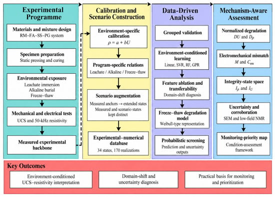
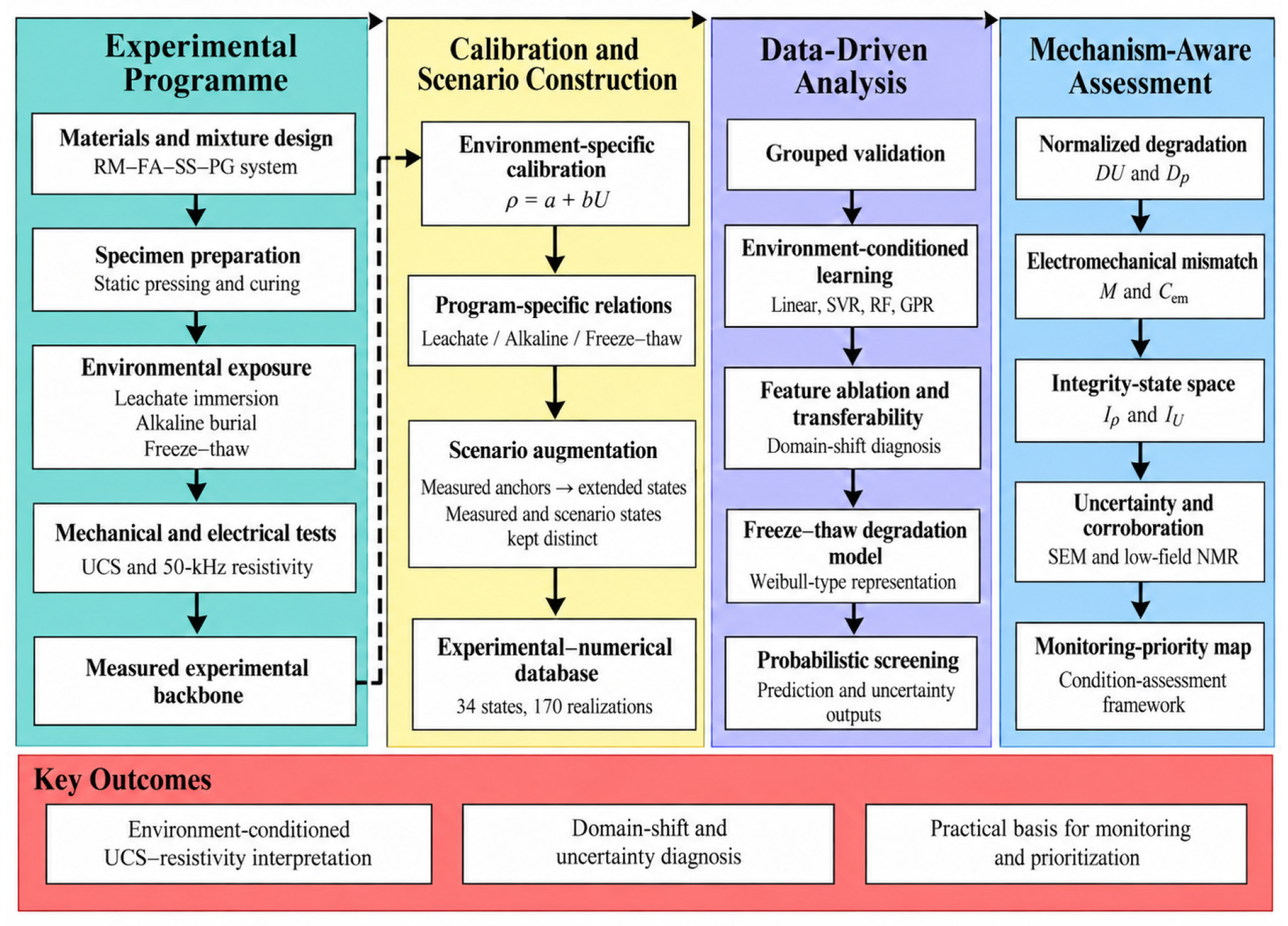
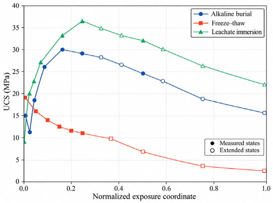
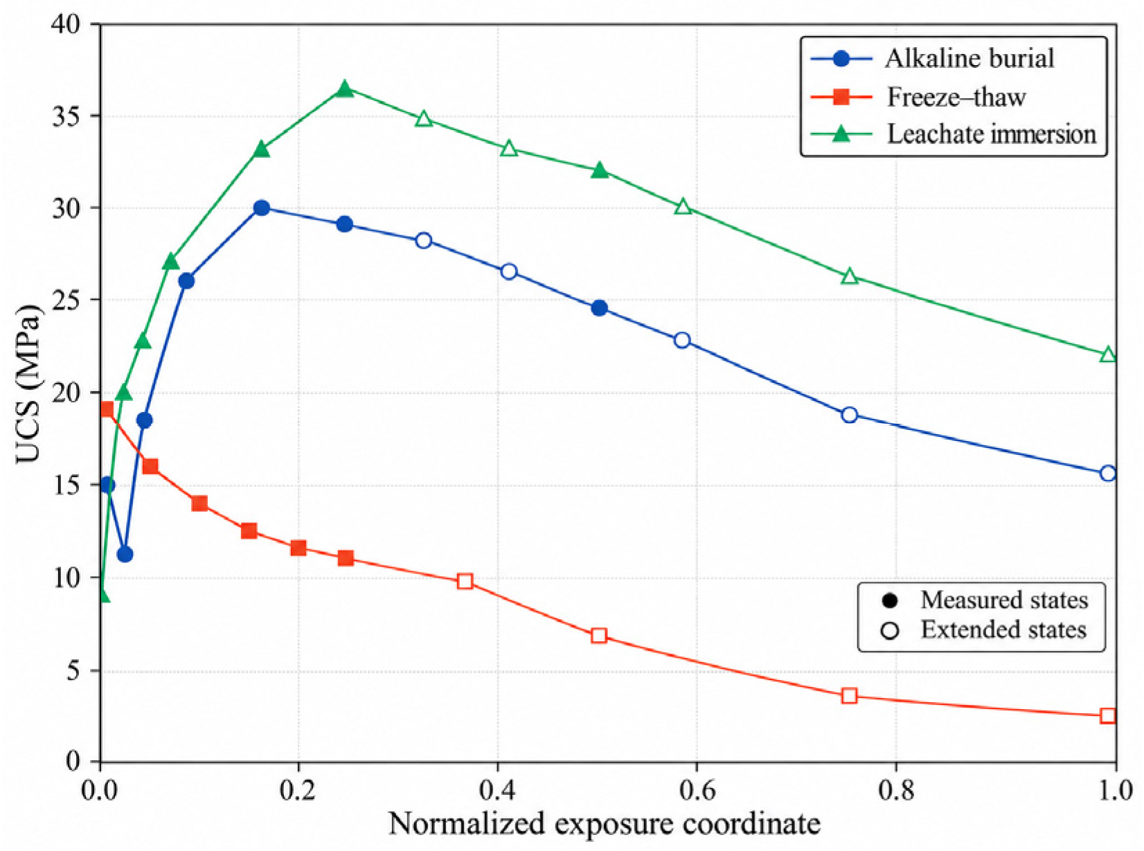
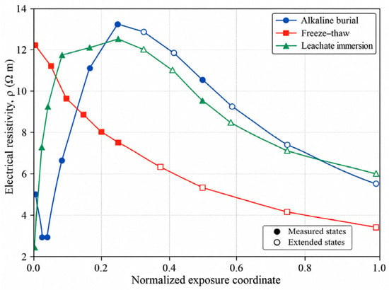
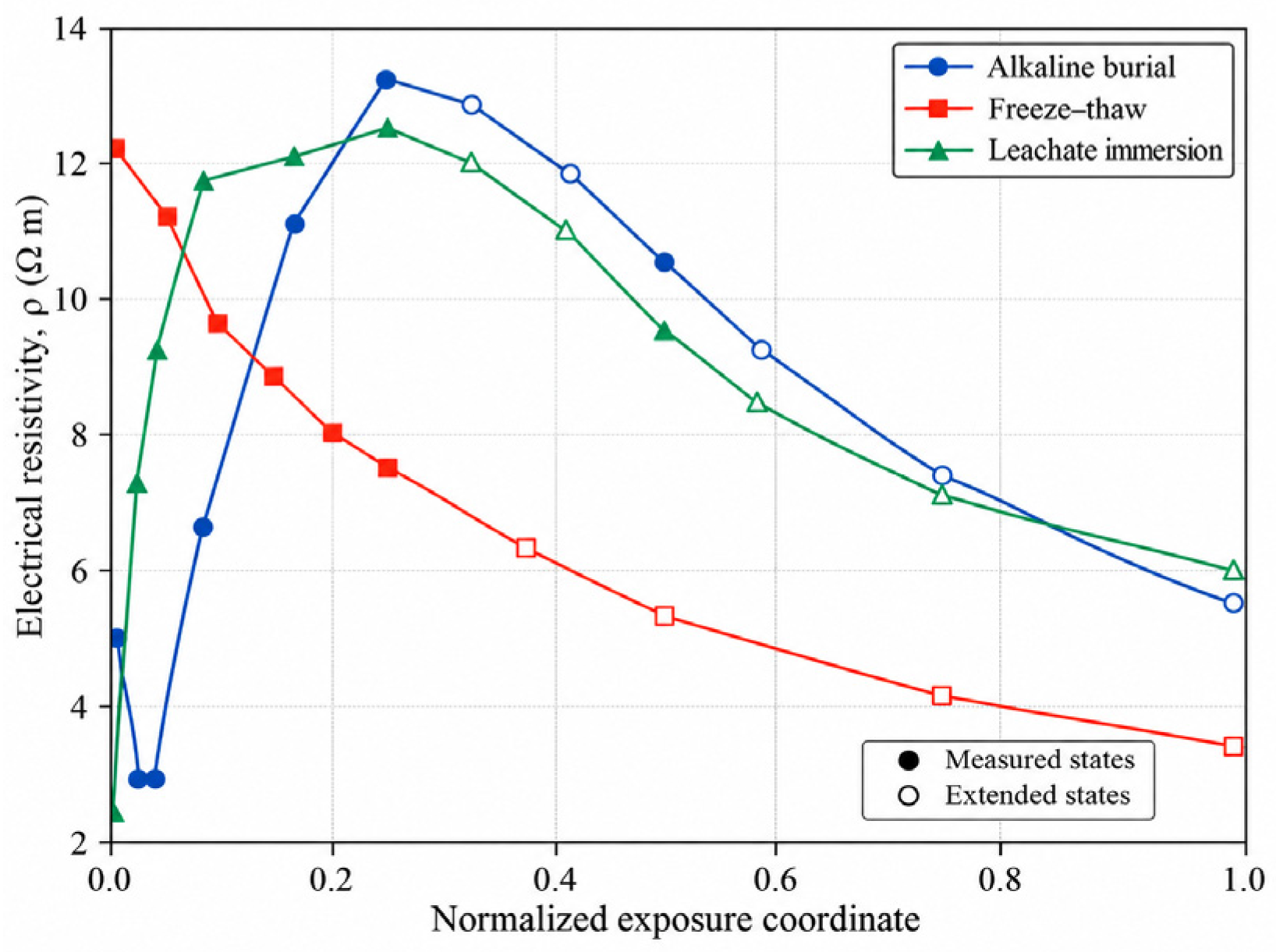
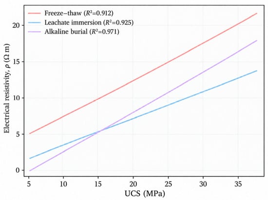
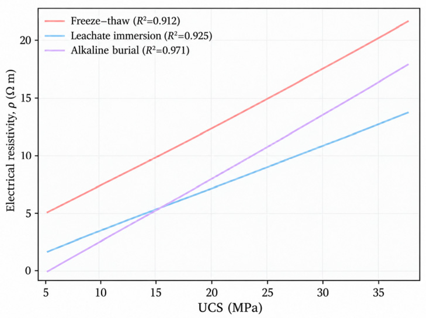
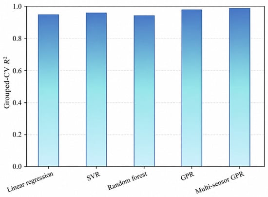
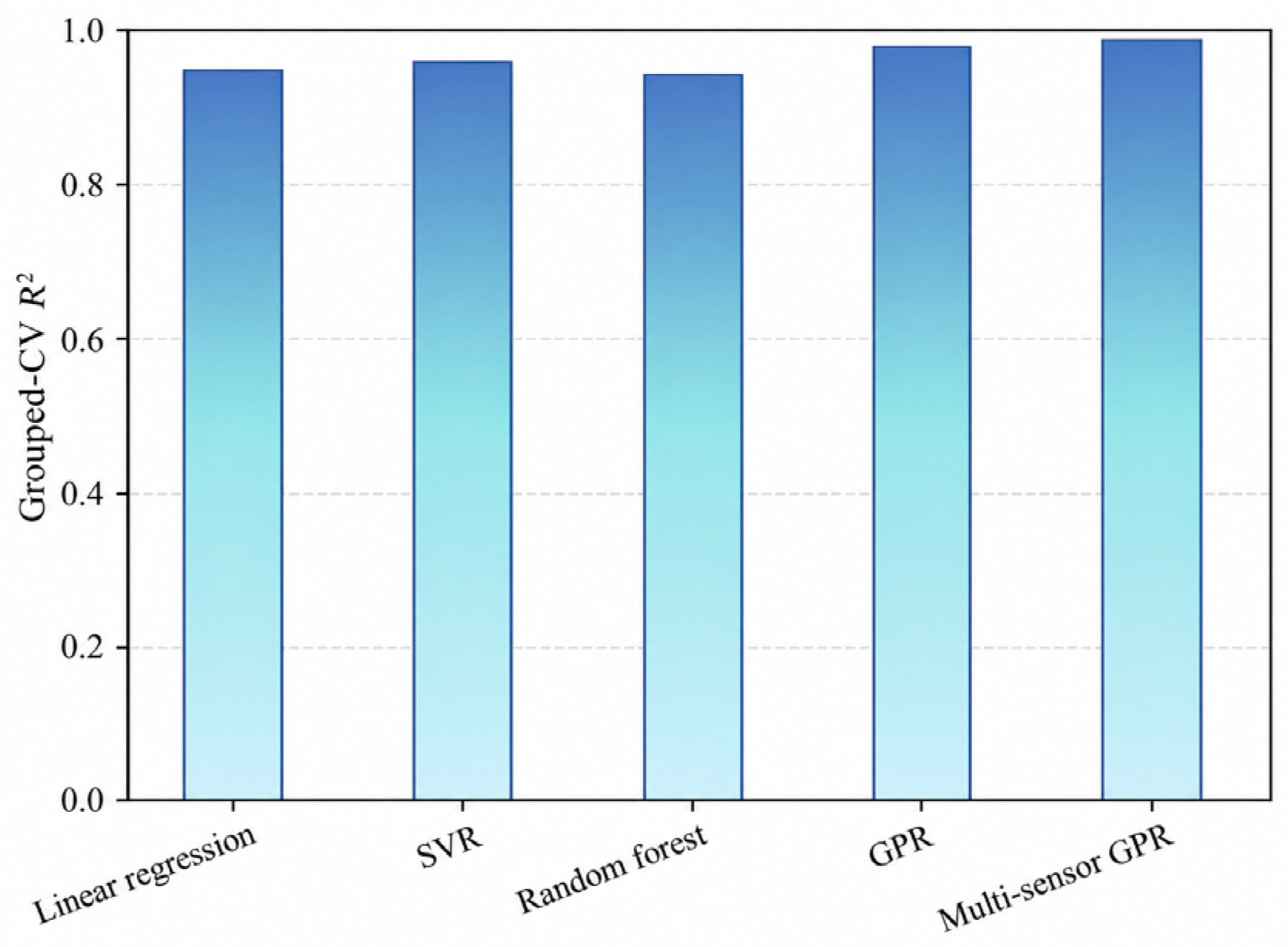
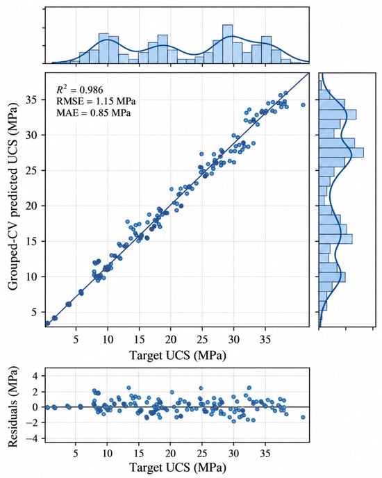
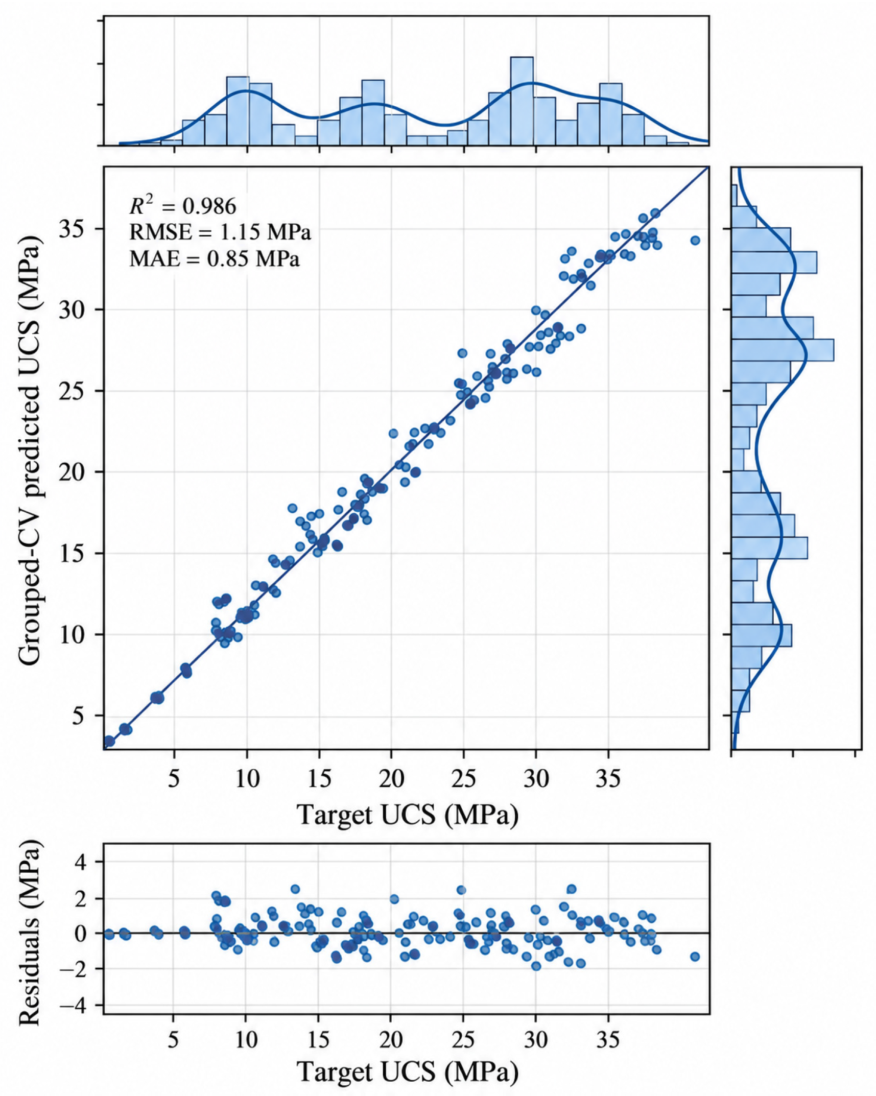
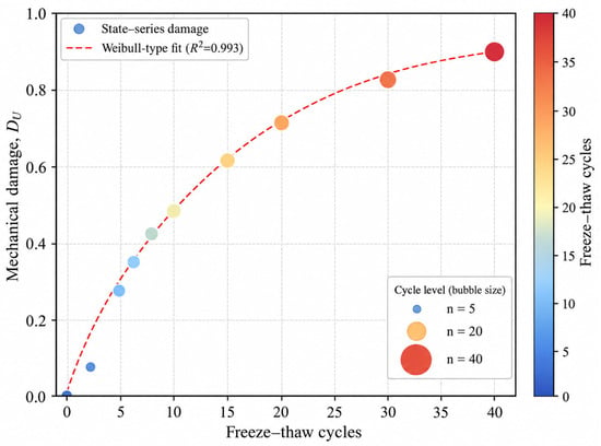
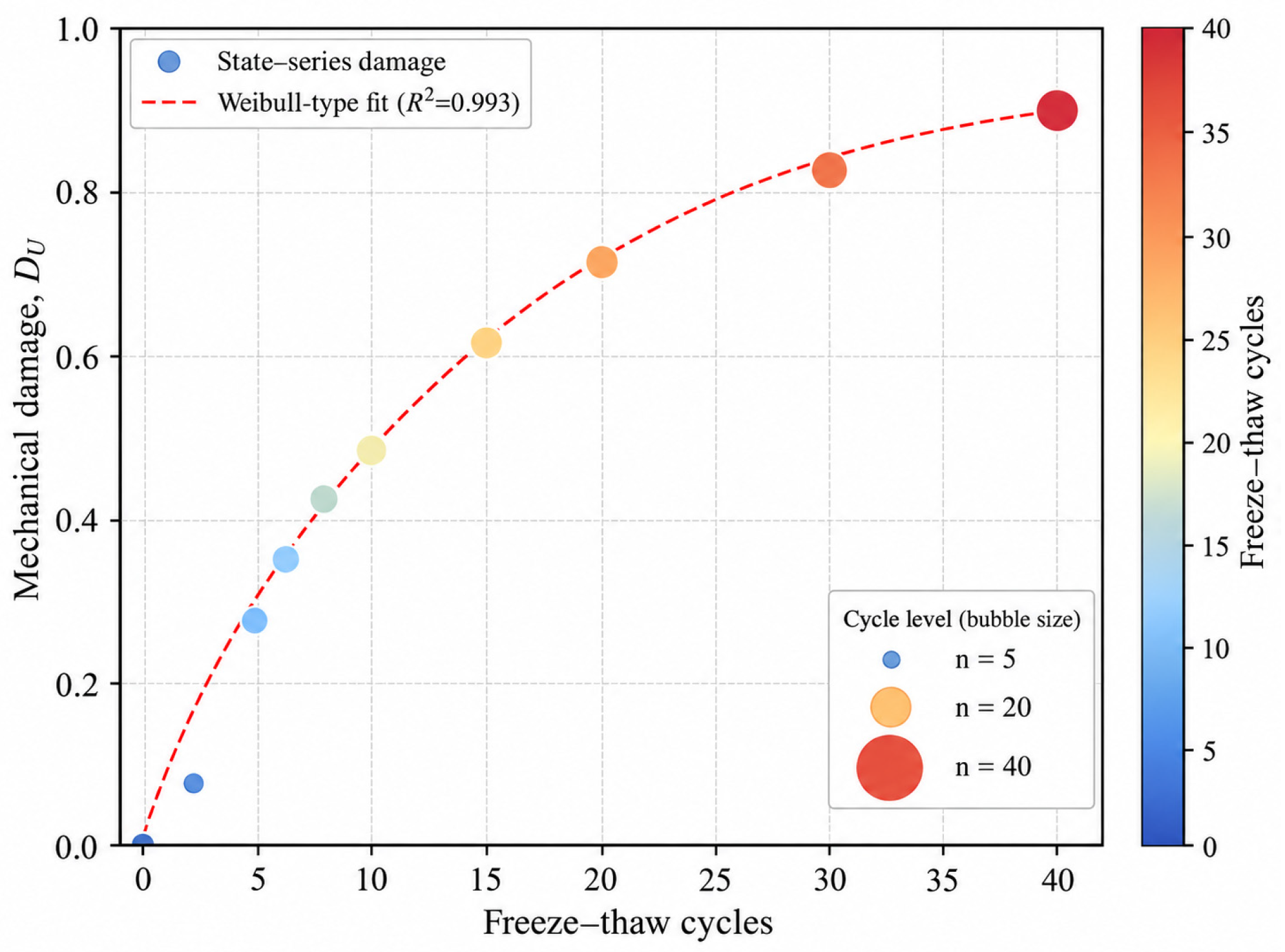
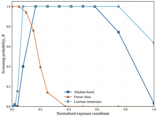
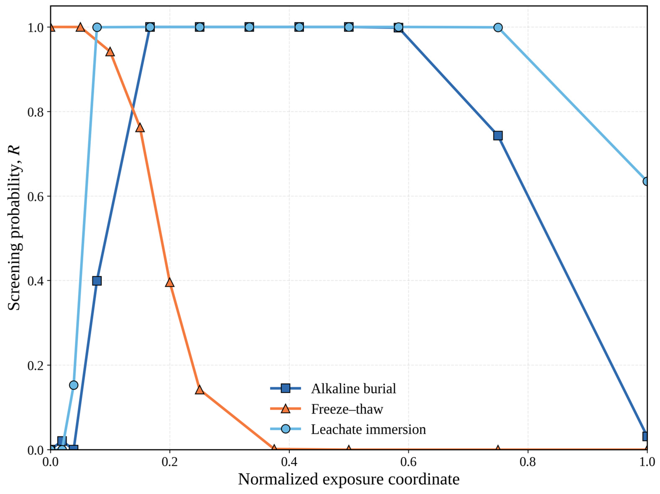
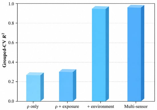
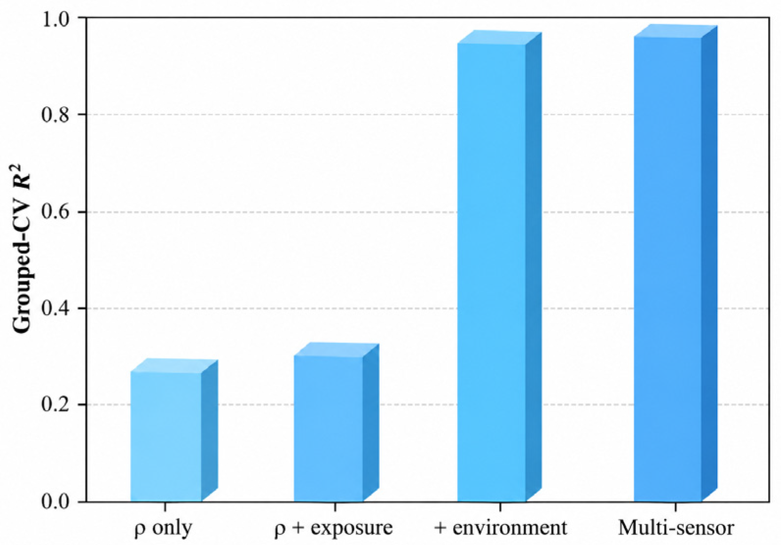
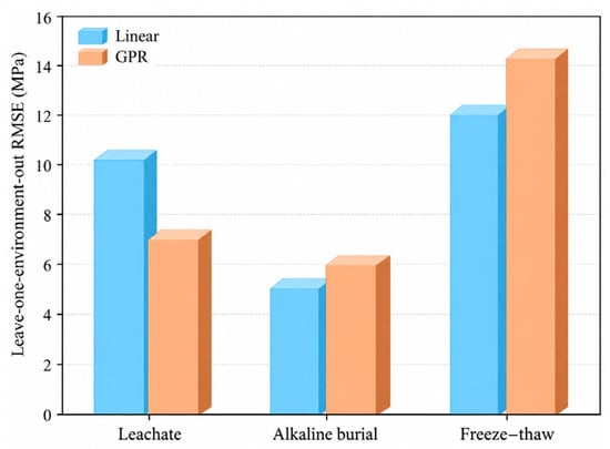
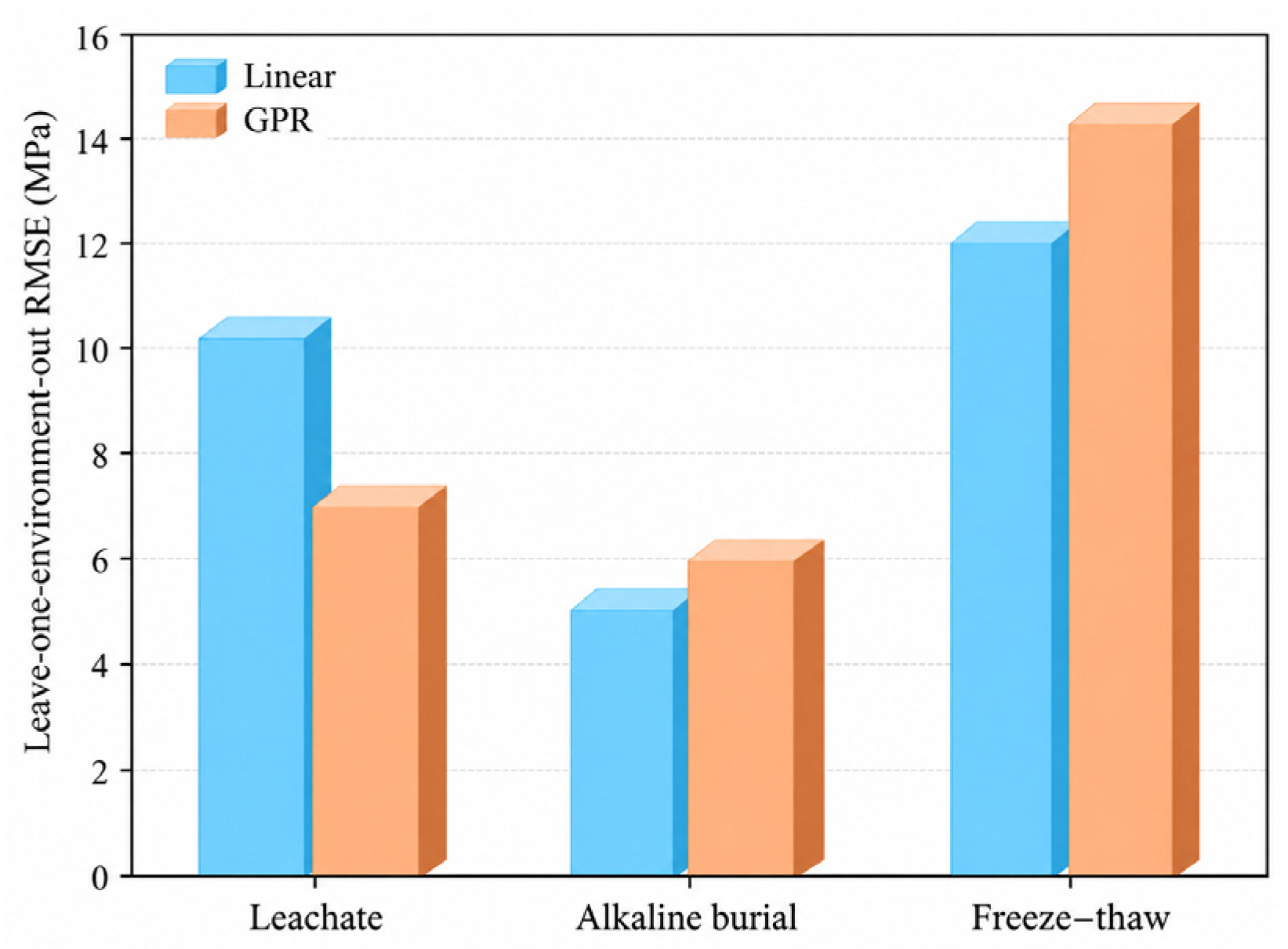
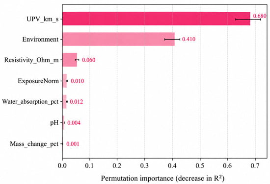
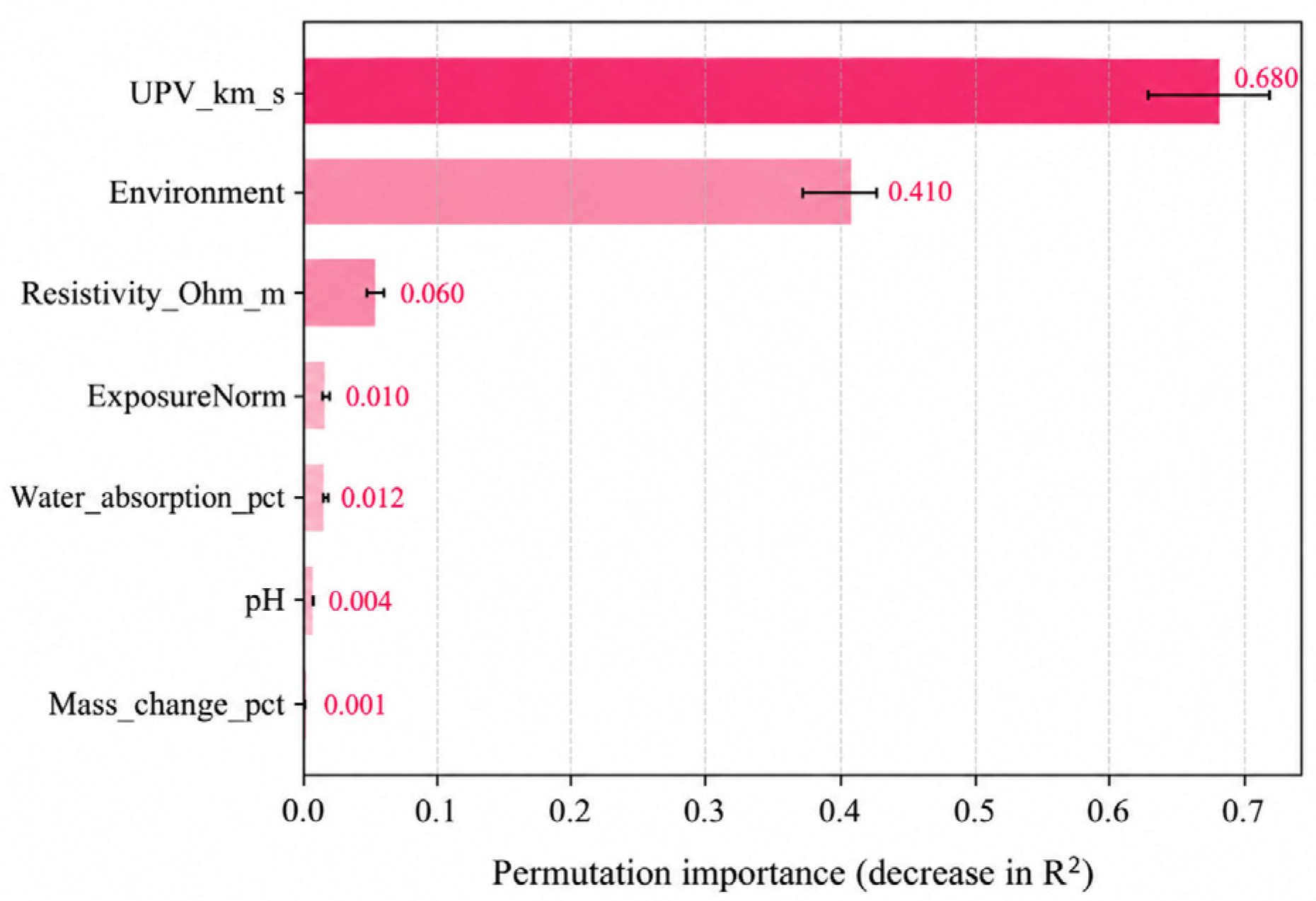
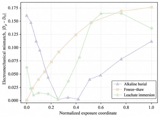
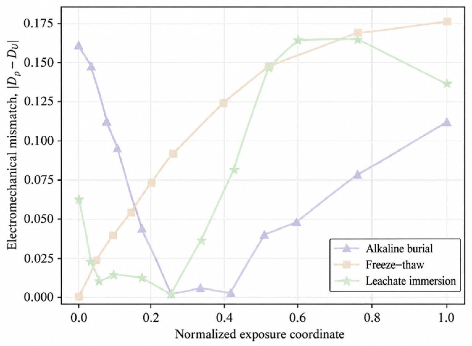
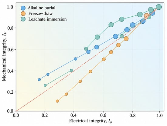
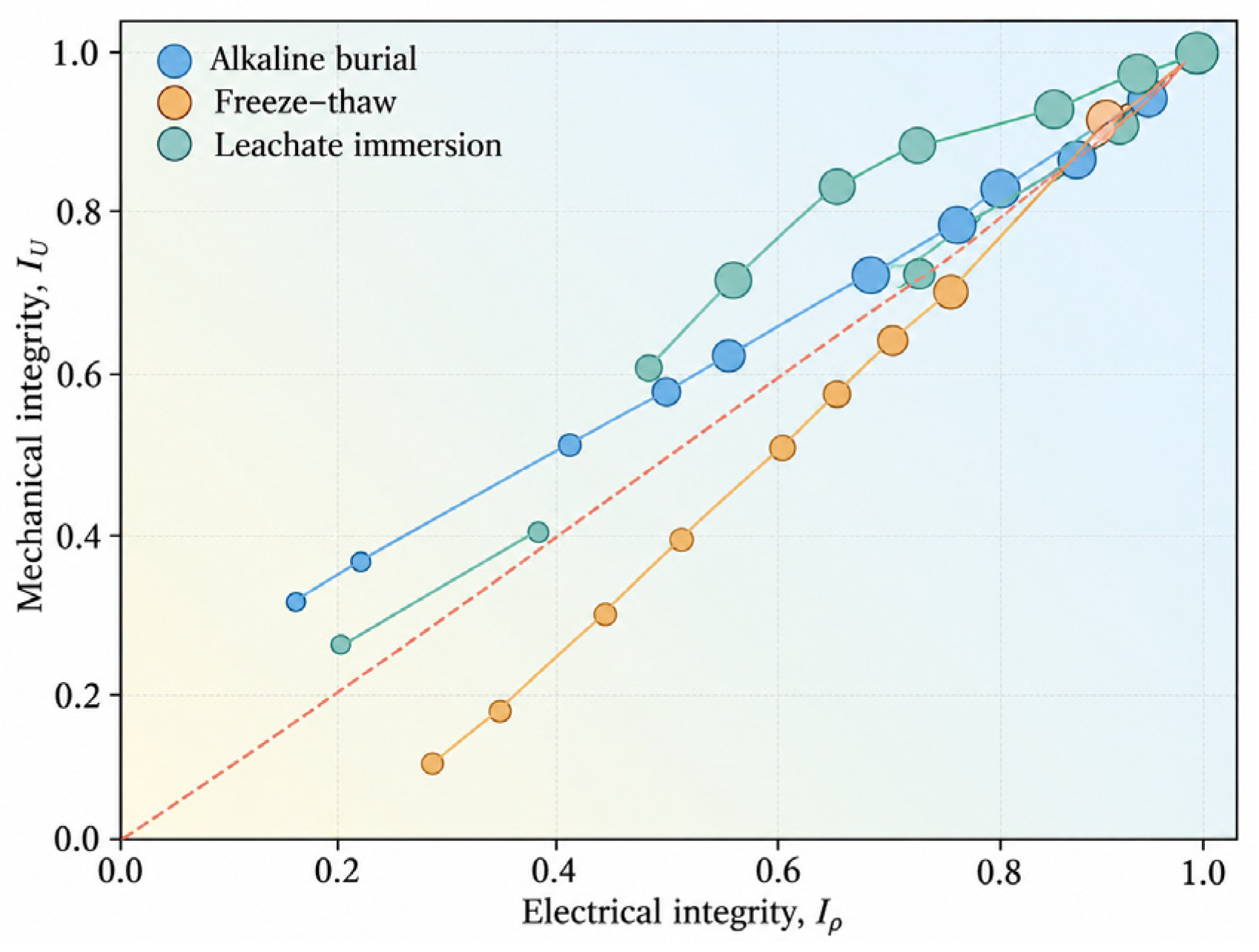
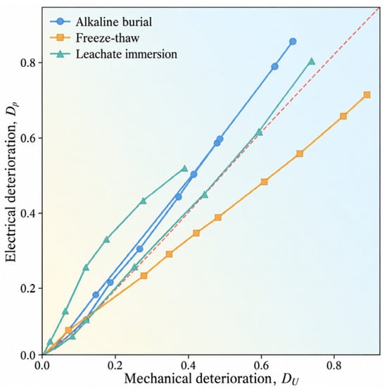
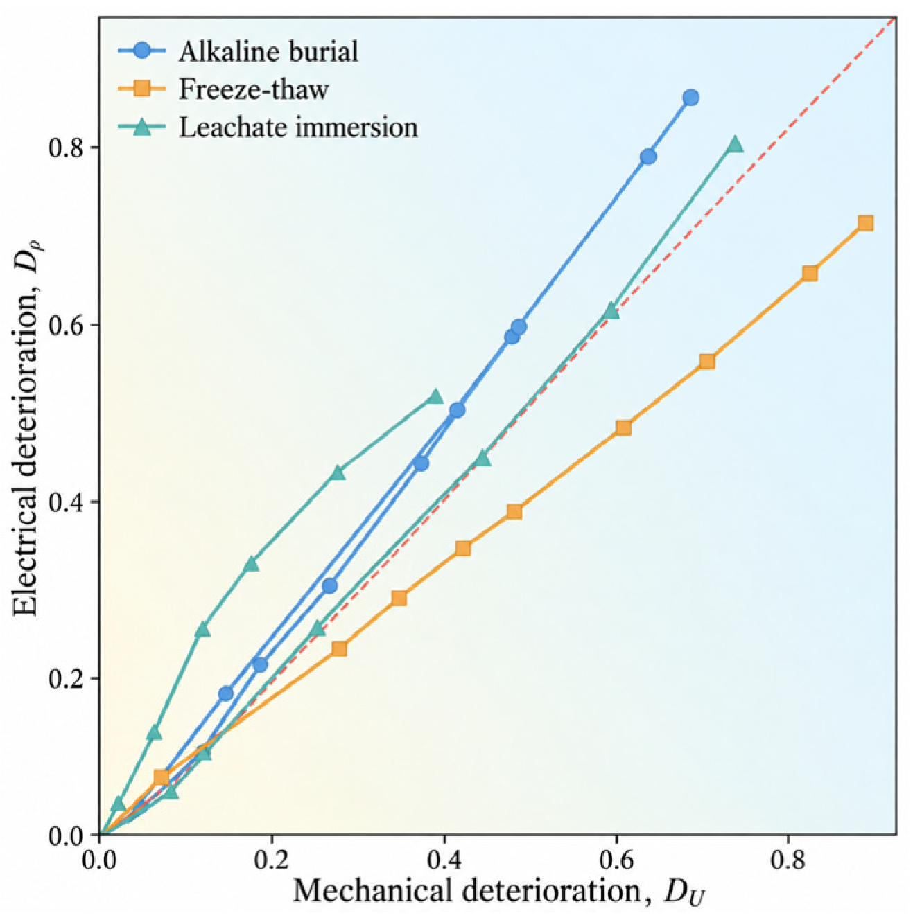
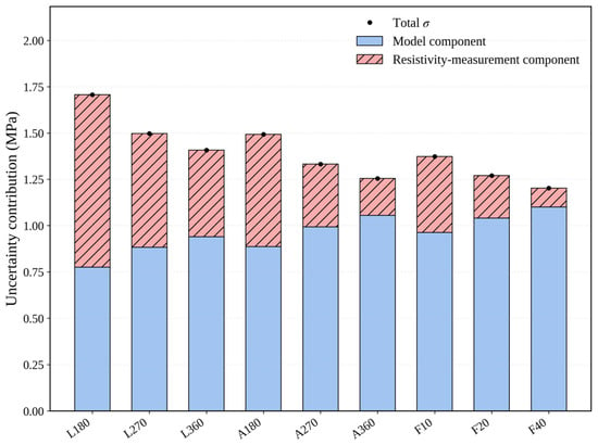
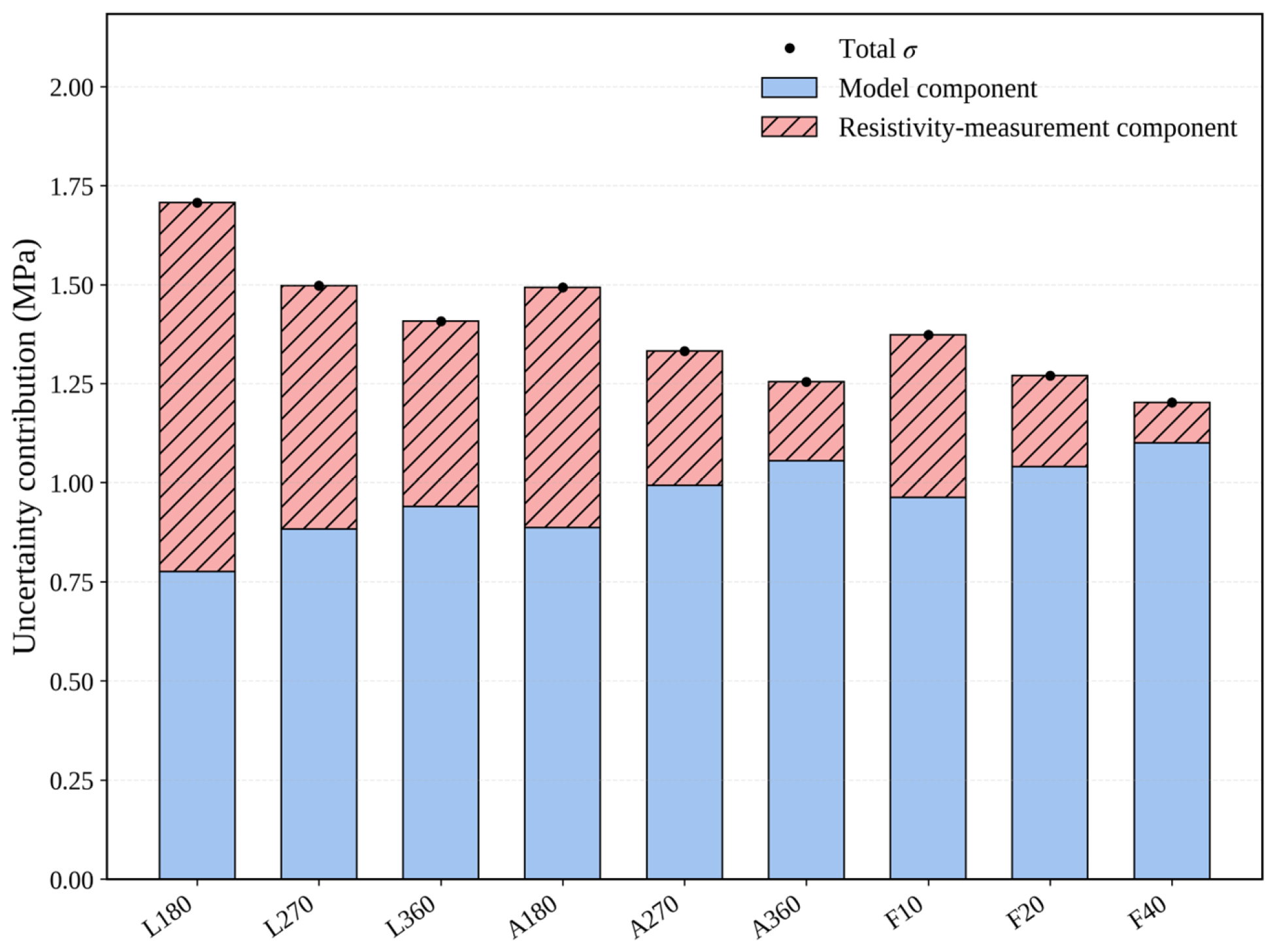
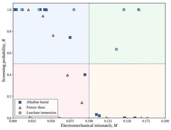
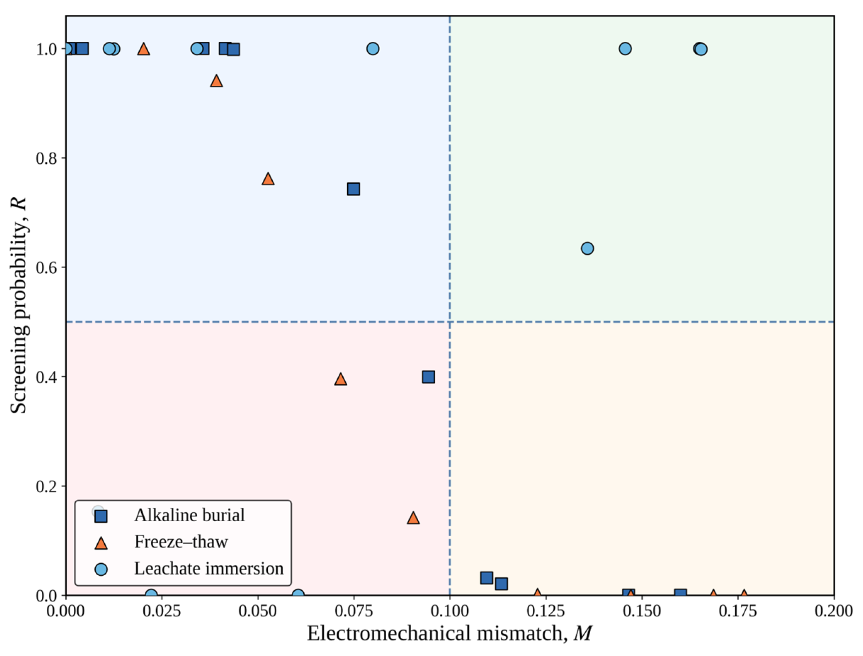
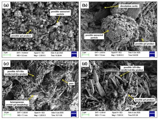
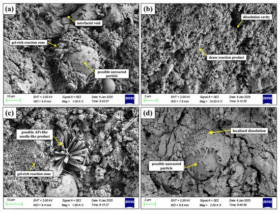
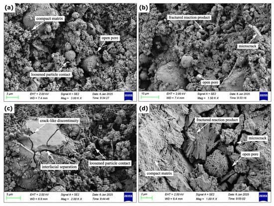
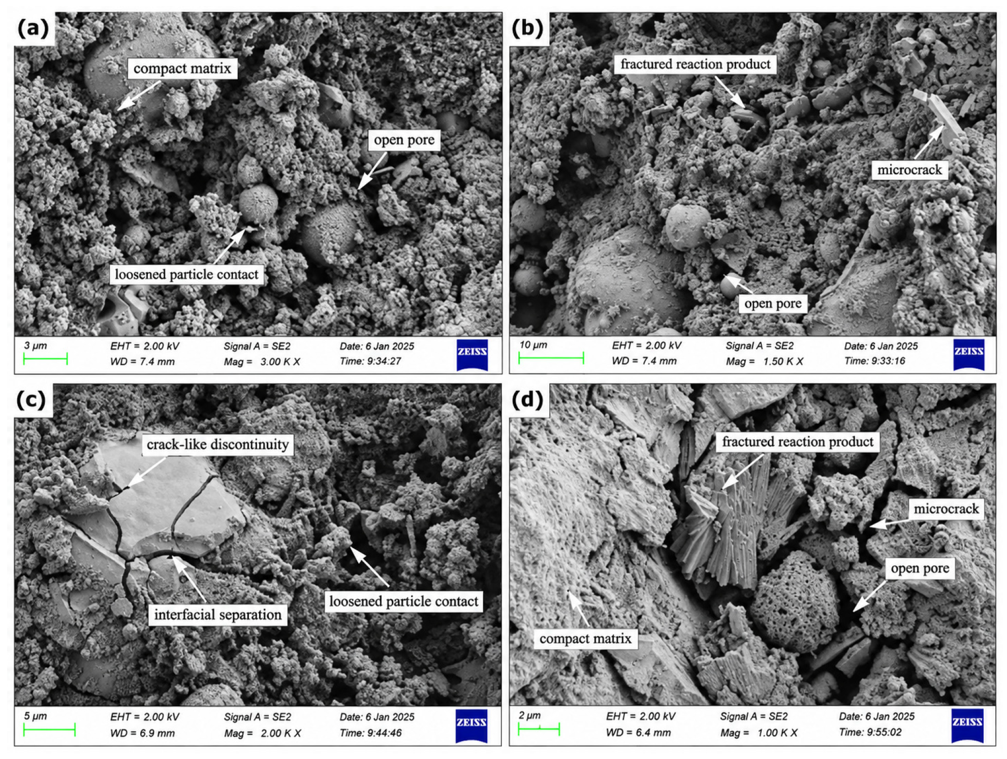
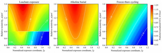
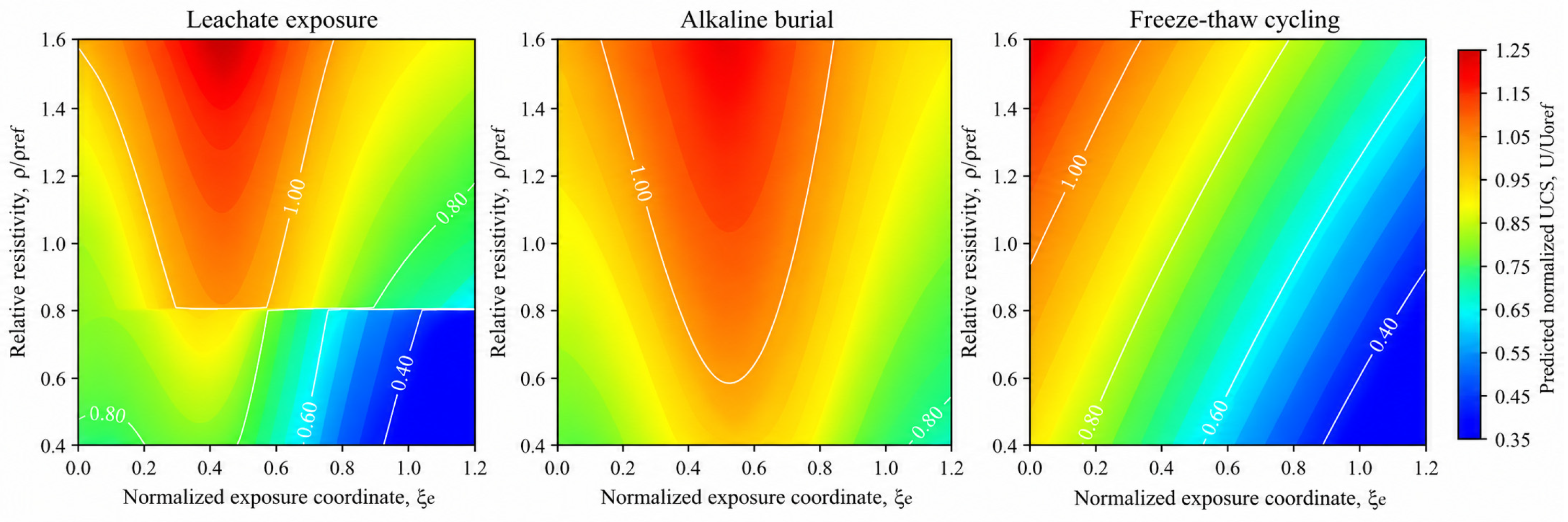
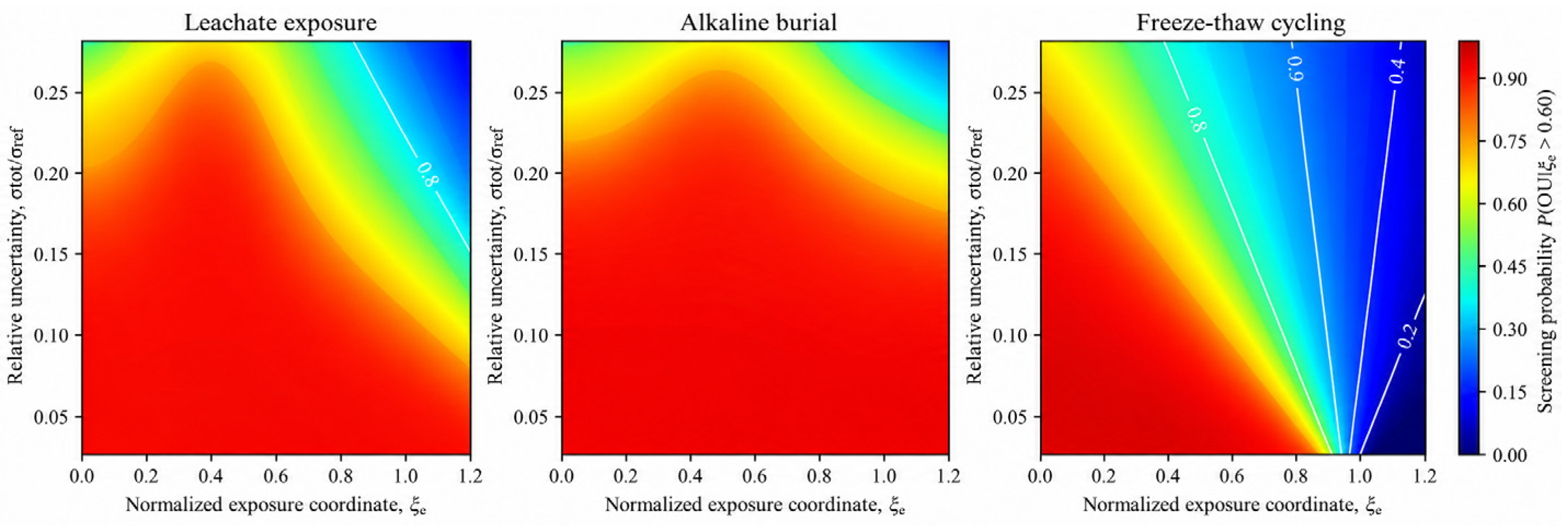
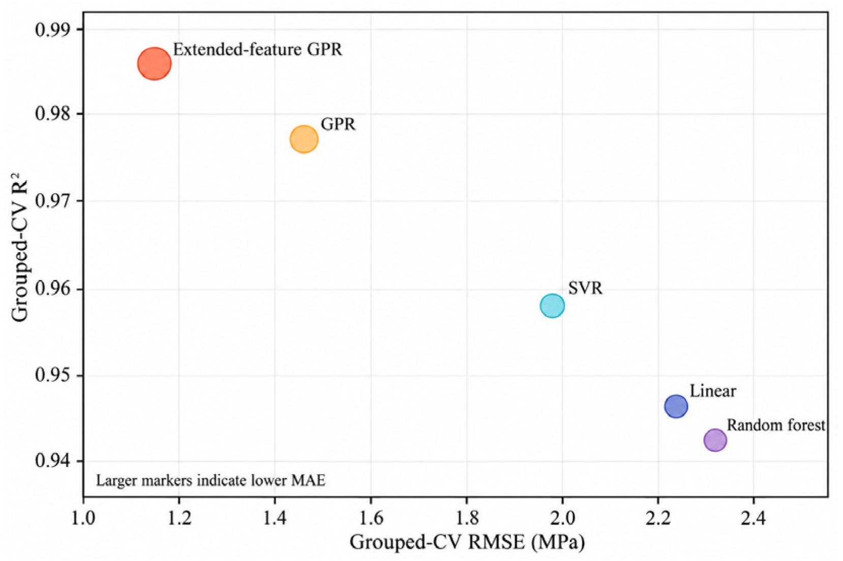
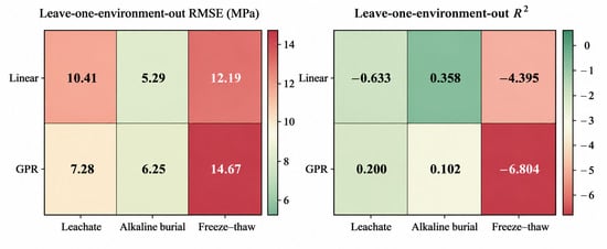
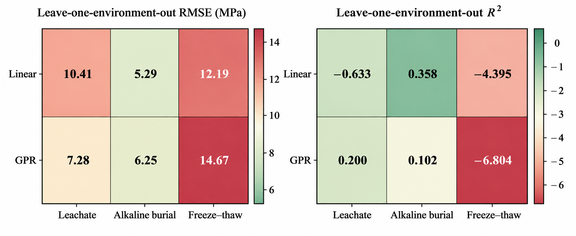
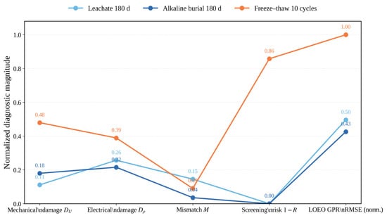
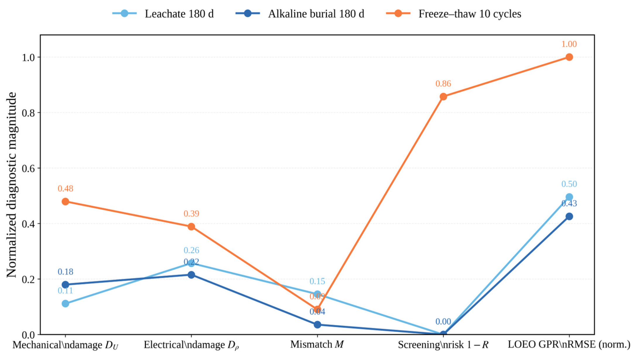



Disclaimer/Publisher’s Note: The statements, opinions and data contained in all publications are solely those of the individual author(s) and contributor(s) and not of MDPI and/or the editor(s). MDPI and/or the editor(s) disclaim responsibility for any injury to people or property resulting from any ideas, methods, instructions or products referred to in the content. |
© 2026 by the authors. Licensee MDPI, Basel, Switzerland. This article is an open access article distributed under the terms and conditions of the Creative Commons Attribution (CC BY) license.