


Abstract
Long-distance water diversion projects are important infrastructure for addressing spatial and temporal imbalances in water resources. However, the construction of complex underground cavern groups involves changing geological conditions, overlapping activities, and interacting risks that challenge conventional static assessment methods. This study applies the work breakdown structure–risk breakdown structure (WBS–RBS) method to identify risks and develop an assessment system comprising 15 indicators across five dimensions: personnel, equipment, materials, methods, and environment. A dynamic risk assessment model integrates the Decision-Making Trial and Evaluation Laboratory (DEMATEL), analytic network process (ANP), variable weight theory, and cloud model. Application to an engineering project identifies geological conditions and equipment operating conditions as key risk drivers. The analysis also identifies plausible influence pathways involving geological deterioration, increased equipment loading, emergency-response pressure, and unresolved hazards. Compared with a static model, the proposed model exhibits a stronger responsiveness to high-risk conditions, with its outputs generally consistent with project management records. Quantitative warning rules and proactive control strategies are proposed to support dynamic monitoring and intervention. The model provides a systematic approach to construction safety risk assessment under uncertainty and a practical reference for risk management in complex underground engineering.
1. Introduction
Water resources are distributed unevenly across time and space worldwide. Severe pollution further limits the effective recycling and reuse of substantial quantities of water, increasing the need for rational water allocation and utilization. Over the past two decades, long-distance water diversion projects have made considerable progress in addressing these imbalances and have provided valuable experience in project planning, design, construction, and operation [1,2]. However, although these projects help alleviate uneven water distribution, they also introduce a range of safety risks. Hydraulic engineering construction typically involves large cross sections, high slopes, deep excavations, extensive construction fronts, and numerous overlapping operations. These projects are undertaken in complex environments where working conditions change rapidly, and construction activities are highly susceptible to hydrological, meteorological, geological, and other natural disturbances [3].
Complex underground cavern groups are critical components of long-distance water diversion projects, accommodating water conveyance facilities, pumping stations, valve chambers, and maintenance passages. Their construction safety directly affects project delivery and long-term operational stability, making them among the most risk-intensive and difficult-to-control components of these projects. Compared with surface and shallow underground sections, underground cavern groups in long-distance water diversion projects frequently traverse complex geological formations and present concealed hazards, including rockbursts, sudden water inflows, collapses, and harmful gas accumulation. Restricted workspaces, dispersed work faces, and limited escape routes increase the risk of accidents that can cause multiple fatalities and injuries, construction delays, cost overruns, and even disruptions to the functionality of the entire diversion system. Large powerhouse caverns and associated tunnels must be excavated in rock masses with spatially variable properties. In mountainous regions, high in situ stress, geological discontinuities, and stress redistribution caused by excavation and unloading can create conditions conducive to rockbursts, large deformation, and collapse. Li et al. [4] reviewed these problems in underground hydropower projects in southwest China, demonstrating the importance of interpreting monitoring results in conjunction with geological conditions and construction activities. These challenges become more pronounced when multiple underground openings are excavated within the same rock mass. Excavation alters the stress distribution and confinement conditions of adjacent structures, while concurrent construction activities compete for access, ventilation, and emergency evacuation routes. Safety assessment must therefore account for an evolving construction system in which hazardous processes interact and influence one another over time.
Despite these challenges, current safety risk management for complex underground cavern group projects remains constrained by insufficient risk quantification, predominantly static control approaches, limited analysis of risk coupling, and inadequate integration with intelligent early warning technologies. To address these limitations, this paper develops a systematic framework for dynamic safety risk assessment based on a representative project involving a complex group of underground caverns. The framework aims to support the systematic identification of hazards, quantitative assessment of evolving risks, and development of targeted risk response strategies. By translating changing construction conditions and associated hazards into identifiable, assessable, and controllable risk factors, the proposed approach provides a basis for more effective preventive measures and safety management throughout construction. The study extends the application of dynamic risk assessment to complex underground engineering and contributes to the development of a systematic framework for evaluating interacting safety risks. In practical terms, effective dynamic risk assessment and timely responses can help prevent or mitigate construction accidents, reduce associated losses, and limit project cost exposure.
2. Literature Review
2.1. Complex Underground Cavern Groups
A complex underground cavern group comprises two or more tunnels, caverns, and associated access passages arranged in intersecting three-dimensional or parallel configurations within geological formations. Such systems typically exhibit at least two interacting characteristics, including large burial depth, large cross sections, high in situ stress, high external water pressure, well-developed karst, and overlapping construction activities. Functionally, these systems include long-distance water conveyance tunnel groups; the three major cavern groups of underground powerhouses, main transformer chambers, and tailrace surge chambers in hydropower stations; and urban underground transportation and integrated municipal hub complexes [5]. Under complex geological conditions and high in situ stress, large underground cavern groups may experience deep rock fracturing, large-scale collapses, extensive sidewall spalling, widespread shear displacement and deformation, and deep-seated relaxation failure.
Research on complex underground cavern groups has primarily focused on achieving safe and efficient construction under conditions of large burial depth, high in situ stress, and complex geology. Microseismic monitoring and support optimization have been used to prevent and control rockbursts, while theoretical analysis, numerical modeling, and field measurements have been combined to develop and evaluate construction techniques. Einstein et al. [6] are widely recognized as pioneers in the systematic introduction of uncertainty and risk analysis into tunnel and underground cavern engineering. Their central argument—that geological uncertainty should be a fundamental consideration in engineering decisions—has influenced subsequent research on quantitative risk assessment. Ren et al. [7] developed a comprehensive safety evaluation method (CsEM) based on two fundamental failure modes: deformation-induced instability of the surrounding rock and collapse of rock blocks. The method supports dynamic early warning and graded risk control. Building information modeling (BIM) and three-dimensional digital technologies have further facilitated the integration of safety risk information across design, construction, and operation into dynamic management systems. These developments have been applied to large hydropower cavern groups, diversion tunnels, and other water conveyance projects. Li et al. [8] investigated construction safety risks in cavern groups using FLAC3D numerical simulation. Xia et al. [9] reproduced stress paths associated with the staged excavation of the Shuangjiangkou powerhouse through laboratory unloading tests. Their results indicate that strength and deformation characteristics depend on the unloading path and that mechanical parameters deteriorate as confining pressure is removed. For construction safety assessment, these findings support stage-dependent modeling and reassessment following bench excavation or substantial changes in support conditions. Kumar and V. R. [10] investigated deformation and support-related instability in the machine hall of the Tala hydropower plant after construction. Although this study provides post-construction evidence rather than a direct test of construction risk prediction, it demonstrates that deformation and damage may persist beyond individual excavation stages, highlighting the importance of maintaining continuity between construction monitoring and subsequent safety assessment.
2.2. Indicators for Construction Safety Risk Assessment in Complex Underground Cavern Groups
A useful indicator system should distinguish between the conditions that generate risk, the observations that reveal changes in risk, and the factors that determine the resulting consequences. Combining these elements into an undifferentiated weighted score can obscure the sources of risk at a particular location and the interventions required to control it. Construction safety risk indicators for underground cavern groups have evolved from experience-based checklists toward more comprehensive and dynamic assessment systems. Conventional scoring approaches have increasingly been supplemented by intelligent algorithms, including entropy-weighted Bayesian networks and LSTM–XGBoost models. At the same time, indicator systems have been expanded into fine-grained monitoring frameworks covering personnel, equipment, materials, methods, and environmental conditions. Approaches to weight determination have also progressed from subjective expert judgment toward game-theoretic methods incorporating interval-valued intuitionistic fuzzy sets. In addition, digital-twin-based dynamic Bayesian networks driven by real-time monitoring data have enabled changes in surrounding rock conditions, support performance, water inflow, and rockburst activity to be incorporated into risk assessment and early warning.
Wang et al. [11] used work breakdown structure–risk breakdown structure (WBS-RBS) analysis to develop an indicator system for mining-method metro tunnel construction and combined fuzzy set theory, the analytic hierarchy process (AHP), and a Bayesian network for risk assessment. Sun et al. [12] used WBS–RBS to identify hazards in metro shield construction, combined G1 and entropy weights through game theory to establish baseline indicator weights, and applied variable weighting and an extension cloud model to classify construction risk. Their study provides a direct precedent for linking work-package hazard identification to state-dependent weighting and cloud-based classification. This paper builds on the approach by deriving the baseline weights from expert judgments about how the indicators influence one another. This allows the daily assessment to account for both an indicator’s importance within the influence network and its observed condition on the assessment day. Zavadskas et al. [13] provided a comprehensive review of multicriteria decision-making (MCDM) methods, covering alternative approaches to indicator weighting, including AHP, the analytic network process (ANP), and entropy weighting. Tah et al. [14] examined a knowledge management framework for construction project risk management, emphasizing the systematic collection, analysis, and application of risk-related information. Xu et al. [15] identified 17 leading indicators, highlighting organizational commitment, participation by clients, designers, and contractors, training, safety climate, and competence. Yang et al. [16] developed a structural equation model based on tunnel accident factors and questionnaire data. Their findings identified significant contributions from human factors, materials, geological exploration, design, technical management, safety management, and natural conditions, thereby linking physical conditions with organizational influences. Wang et al. [17] combined structural equation modelling with a fuzzy cognitive map to assess risks in mining-method metro construction. Their case study emphasized excavation and advanced support, including excavation footage, excavation sequence, and over-excavation or under-excavation. These findings support the association of risk indicators with specific construction processes and activities.
The principal methodological contribution is the integration of network-derived baseline weights with a threshold-based adjustment for daily indicator states. The contribution of this adjustment is to compare daily classifications under fixed and state-adjusted weights while holding the observations, cloud parameters, and grading rule constant. The engineering contribution lies in applying this procedure to the underground cavern groups, where the indicators represent hazards identified across construction work packages and are assessed using site monitoring data and management records.
2.3. Methods for Construction Safety Risk Assessment in Complex Underground Cavern Groups
Construction safety risk assessment for complex underground cavern groups has increasingly moved beyond conventional static, single-dimensional analysis toward dynamic approaches that account for nonlinear relationships and support intelligent decision-making. These approaches include the Decision-Making Trial and Evaluation Laboratory-based analytic network process (DANP), variable weight theory, and cloud models. They address three principal challenges: strong coupling among indicators, changes in indicator importance over time, and uncertainty in risk information. Integration with Bayesian networks and deep learning further provides opportunities to move from retrospective analysis toward prospective risk assessment and early warning.
By incorporating the Decision-Making Trial and Evaluation Laboratory (DEMATEL) method, DANP establishes a directed influence network among indicators. In addition to calculating indicator weights, it identifies influential factors through measures of prominence and net influence. However, baseline weights obtained using DANP have a limited capacity to accommodate abrupt changes in construction risk conditions. Variable weight theory addresses this limitation by introducing a state-dependent weighting function that adjusts indicator weights based on the observed state of the system, increasing the weight assigned to indicators that exhibit deterioration when appropriate. Saaty et al. [18] elaborated network-based decision theory for elements characterized by interdependence and feedback. Hsu et al. [19] presented a representative application of DANP in decision science, demonstrating how DEMATEL and ANP can be combined to address complex decision-making problems. Ren et al. [7] developed a comprehensive method for evaluating the safety of surrounding rock in complex underground cavern group construction, enabling dynamic, quantitative assessment of rock stability during construction.
For risk classification, the cloud model uses three numerical characteristics—expectation, entropy, and hyperentropy—to establish a bidirectional transformation between qualitative concepts and quantitative data while accounting for uncertainty. Li et al. [20] formally proposed this model for representing uncertainty in such transformations. Yang et al. [21] developed the cloud Delphi hierarchical analysis method, integrating cloud models to address uncertainty in expert judgments. Their work provides methodological guidance on handling uncertainty in subjective judgments during the expert survey conducted in this study. Wang et al. [22] applied cloud models to multicriteria group decision-making in uncertain linguistic environments, demonstrating their capacity to accommodate both fuzziness and randomness in assessment information. Accordingly, this paper adopts a cloud model for comprehensive risk classification.
Considerable progress has been made in dynamic construction safety risk assessment for complex underground cavern groups. Indicator systems have expanded from individual geological or structural measures to multidimensional frameworks covering personnel, equipment, materials, methods, and environmental conditions. Microseismic monitoring, BIM, geographic information systems (GIS), and the Internet of Things (IoT) have facilitated the acquisition of more detailed and timely indicators. Assessment methods have progressed from qualitative scoring to quantitative modelling, and from static evaluation to dynamic early warning. Intelligent approaches, including Bayesian networks, deep learning, and cloud models, have provided additional means of improving assessment accuracy and timeliness. Risk response has also shifted from reactive intervention toward preventive management, with digital twins and knowledge graphs offering further opportunities for intelligent risk identification and timely response.
Nevertheless, existing research has focused primarily on metro tunnels and hydropower caverns, with limited systematic investigation of risks specific to deeply buried, long-distance, high-water-pressure diversion tunnel groups. Examples include ventilation challenges over long construction distances and interactions between tunnel boring machines (TBMs) and hard rock. In addition, many studies rely on assumptions of indicator independence or provide insufficient characterization of interdependent risk relationships. Static weights are also poorly suited to changing construction conditions because they cannot readily reflect real-time changes in the relative importance of risk factors arising from abrupt geological changes or equipment failures. These limitations may reduce the responsiveness of assessment systems and delay the identification of emerging risks.
To address these limitations, this paper investigates the dynamic assessment of construction safety risks for complex underground cavern groups. A WBS–RBS-based risk identification system is developed, followed by an assessment framework integrating DANP, variable weights, and a cloud model. The proposed framework is intended to support dynamic risk identification, quantitative assessment, and intelligent early warning, thereby providing theoretical support and practical guidance for improving construction safety.
3. Development of Indicators for Dynamic Construction Safety Risk Assessment
3.1. Construction Safety Risk Identification Based on WBS–RBS
The Work Breakdown Structure (WBS) decomposes the construction scope into manageable work packages, while the Risk Breakdown Structure (RBS) organizes potential sources of risk. Combining these structures enables the systematic identification of risk sources associated with individual construction activities, providing a structured basis for hazard identification and the development of corresponding assessment indicators. The WBS–RBS approach supports comprehensive risk coverage and traceability [23]. For complex underground cavern group projects involving complicated operations, intersecting underground spaces, and interdependent risks, this approach helps reduce omissions that may arise from conventional experience-based identification. By systematically examining construction activities and their associated risk dimensions, it provides an adaptable framework for identifying hazards across different work interfaces.
3.1.1. WBS–RBS Risk Association Matrix
The WBS was developed based on project construction organization plans and interviews with project technical managers. The RBS was structured around five dimensions: personnel, equipment, materials, methods, and environment (4M1E), drawing on the relevant literature. To support systematic and reliable risk identification, this study developed a WBS–RBS workflow that combines structural decomposition with risk verification, drawing on multiple information sources. As shown in Figure 1, three types of data were used for cross-validation.
Figure 1.
WBS–RBS risk identification workflow.
Drawing on numerous construction organization plans and tender drawings for underground cavern groups, the WBS hierarchically decomposed the project into seven primary stages, including construction preparation, deep excavation, and main tunnel construction. These stages were further divided into 31 manageable work packages. Table 1 presents the two-level WBS organized by construction stage and principal work content.
Table 1.
WBS decomposition of the underground cavern group project.
The RBS was used to systematically identify and classify potential risks across five categories: personnel, equipment, materials, construction methods, and environmental conditions. Relevant safety management standards and specifications were consulted to establish an initial RBS comprising 5 dimensions and 24 risk factors. To address potential overlaps among risk factors and improve the completeness and reliability of the risk inventory, three-way cross-validation was conducted using the following sources: (1) semistructured questionnaires and interviews with site supervisors, safety officers, and key workers; (2) a project management and technical coordination meeting involving technical representatives from the owner, supervision consultant, and general contractor, with formal minutes documenting the discussions; and (3) expert review by specialists in rock mechanics, hydraulic tunnels, geotechnical investigation and design, and underground engineering risk. This process aimed to establish a comprehensive and reliable inventory of construction hazards associated with the underground cavern group, providing a sound data foundation for subsequent dynamic risk assessment and control, as shown in Table 2.
Table 2.
RBS risk decomposition of the underground cavern group project.
Based on Table 1 and Table 2, each work unit was matched with each safety risk factor to construct an initial matrix comprising 744 assessment cells (31 × 24). Each cell represented a specific risk proposition: whether a particular risk factor was present in a given work package. The resulting two-dimensional WBS–RBS matrix linked construction work units to potential risk factors, providing a systematic basis for identifying and screening construction safety risks. Each risk proposition was assessed using a binary classification: Y denotes a work-package–hazard combination retained after screening and review. N denotes a combination that was not retained. A N entry alone does not establish that the hazard is absent or that its potential consequences are negligible. This classification supported the systematic screening and prioritization of risk propositions for subsequent review.
Round 1: Questionnaire screening by frontline workers. Structured questionnaires were distributed to 84 frontline workers, presenting all 744 risk propositions in clear and accessible language. Based on their work experience, respondents were asked to indicate whether each risk had occurred or was highly likely to occur in an operation for which they were responsible or with which they were familiar (Y), or was essentially absent (N). The questionnaire survey is based on a face-to-face forum and the valid questionnaires accounted for nearly 98%. Then, the number of Y responses was counted for each cell. A preliminary screening threshold was established: a minimum of three Y responses for a proposition to proceed to the next review round. This initial screening identified 52 potentially high-risk cells for further assessment.
Round 2: Detailed review through a joint project management and technical meeting. A six-member assessment group was convened, comprising the owner’s project chief engineer and engineer, safety supervision engineer, chief supervision engineer, and the contractor’s project manager, and technical manager (Table 3). The selection criteria required an associate senior or higher professional title, or equivalent professional registration; at least eight years of relevant research or practical experience; and representation of key organizational stakeholders involved in the project. These criteria were intended to ensure that the assessment incorporated a range of technically informed and practically relevant perspectives. The group reviewed each of the 52 preliminary risk propositions individually, cross-checking construction logs and accident or hazard registers for historical evidence, design drawings and geological investigation reports for geological justification, and construction method statements and verification calculations for the technical plausibility of method- and equipment-related risks. Based on this documentary evidence and the associated management records, the group eliminated unsupported propositions, clarified relevant details, and refined the preliminary findings. 15 propositions arising from individual misunderstandings or involving extremely low probabilities were rejected. For each confirmed risk, the group documented the triggering scenario, potential consequences, and existing control measures. This review yielded 37 key risk cells, with detailed descriptions jointly verified from technical and management perspectives.
Table 3.
Risk assessment panel after preliminary questionnaire screening.
Round 3: Final independent review by external experts using the Delphi method. Five external experts who were not directly involved in project construction were invited to participate (Table 4). The selection criteria included an associate senior or higher professional title, such as professor or senior engineer, or equivalent professional registration, together with at least ten years of relevant research or practical experience. These criteria were intended to ensure that the review incorporated experienced, independent, and practice-oriented perspectives. Two rounds of Delphi consultation were conducted. The 37 risk propositions and detailed background materials from Round 2 were distributed anonymously to the experts for independent assessment. This procedure was intended to reduce potential blind spots and entrenched assumptions within the project team, incorporate independent expert judgment into the final decisions, and strengthen the credibility and potential applicability of the identification results. In the first round, experts independently assessed the existence of each risk and the accuracy of its description, and proposed revisions where necessary. The research team then circulated an anonymous summary of the results, including mean scores and areas of disagreement, together with revised risk descriptions. A proposition was accepted when more than 80% of the experts endorsed it, corresponding to at least four of the five experts. All 37 propositions passed the final review. The reported expert consensus rate was 89.2%, indicating a high level of professional agreement with the identified risks.
Table 4.
The five external experts participating in the Delphi review.
The WBS–RBS matrix for construction preparation (W1) is presented in Table 5. Eight risk points were identified across the personnel, equipment, and environmental dimensions. For personnel-related risks, the traffic diversion unit was associated with noncompliant instructions or operations (R13), including vehicle entry and exit without guidance, vehicle rollaway incidents, and collisions. Management deficiencies (R14) included the use of unapproved traffic diversion plans and the implementation of facilities without acceptance inspection. Temporary works were associated with noncompliant instructions or operations (R12 and R13), particularly unauthorized wiring of temporary electrical supplies and unqualified personnel performing electrical work. For equipment-related risks, utility relocation involved electrical installation defects (R24), including damaged cables, electric shock hazards, and inadequate grounding. Temporary works also posed electrical hazards (R24), including unprotected cables and insufficient clearance from external power lines. For environmental risks, utility relocation involved explosion hazards (R54), particularly in extreme scenarios involving damage to buried gas pipelines. Dewatering tests were associated with abrupt changes in groundwater levels (R52), which could trigger secondary geohazards, including surface settlement.
Table 5.
WBS–RBS matrix for construction preparation.
Table 6 presents the WBS–RBS matrix for deep excavation and working shaft construction (W2). Four risk points were identified across the personnel, equipment, and construction method dimensions. For personnel-related risks, the monitoring unit was associated with management deficiencies (R14), including delays in monitoring data reporting and ineffective warnings, which could prevent the timely identification and management of hazardous conditions. For equipment-related risks, the support unit involved equipment overloading (R22), including incorrectly installed steel struts and excessive loads that could compromise the support structure’s stability. For construction method-related risks, the support unit was associated with inadequate or untimely support parameters (R42), including insufficient support strength and the potential for collapse due to delayed support installation. The excavation unit was associated with process failures (R44), including soil collapse and the burial of personnel.
Table 6.
WBS–RBS matrix for deep excavation and working shaft construction.
Table 7 presents the WBS–RBS matrix for main tunnel construction (W3). Eight risk points were identified across the equipment, materials, construction methods, and environmental dimensions. For equipment-related risks, shield tunneling was associated with inadequate equipment capacity or equipment failure (R21), including lifting injuries during shield assembly or dismantling, cutterhead jamming, and screw conveyor blowouts. Secondary lining operations were similarly associated with inadequate equipment capacity or failure (R21), including formwork detachment, falling objects during concrete placement, formwork blowouts, and support system instability. For material-related risks, waterproofing operations involved material quality defects or price fluctuations (R31), particularly damaged waterproofing membranes and inadequately secured overlaps that could result in leakage. For construction method-related risks, initial support was associated with unreasonable design (R43), including incorrectly installed steel ribs and delayed support installation, reflecting potential discrepancies between design requirements and construction practices. Backfill grouting involved inadequate or untimely parameters (R42), including uncontrolled grouting pressure that could damage lining segments. For environmental risks, drill-and-blast excavation was associated with adverse geological conditions (R51) and explosion hazards (R54). The former involved unstable surrounding rock and inadequate advance geological prediction, whereas the latter concerned blasting-induced vibrations that could affect existing railways, gas pipelines, and other infrastructure. Protection of existing facilities involved potential impacts on residents (R55), primarily through deformation of railways, roads, and pipelines caused by tunneling beneath these facilities.
Table 7.
WBS–RBS matrix for main tunnel construction.
Table 8 presents the WBS–RBS matrix for vertical transportation and muck removal (W4). Four risk points were identified across the personnel and equipment dimensions. Under personnel factors, off-site spoil haulage involved noncompliant instructions or operations (R13), including overloaded trucks and spoil spillage onto roads. These conditions could increase traffic risks, cause environmental pollution, and result in administrative penalties. Emergency access was hampered by management deficiencies (R14), such as blocked access routes and unclear signage, which could delay rescue operations and worsen the consequences of accidents. Under equipment factors, the installation and dismantling of lifting equipment involved process failure (R21), including inappropriate installation and dismantling plans, nonstandard procedures, and deficiencies in electric-grab muck-removal operations. These deficiencies could result in lifting-related injuries, falling loads, and equipment overturning. In-tunnel transportation involved inadequate or untimely operating parameters (R25), including inappropriate operating settings for battery locomotives and poorly coordinated transport operations. These conditions could cause runaway incidents, collisions, and crushing injuries, with particularly serious consequences in confined underground cavern spaces.
Table 8.
WBS–RBS matrix for vertical transportation and muck removal.
Table 9 presents the WBS–RBS matrix for transportation and traffic safety (W5). Three risk points were identified across the personnel and equipment dimensions. Under personnel factors, approval of traffic diversion plans involved management deficiencies (R14), including unapproved plans and facilities that had not undergone acceptance inspections, leaving diversion activities without the required basis for compliance. Road reinstatement acceptance also involved management deficiencies (R14), including substandard reinstatement work and perfunctory acceptance inspections. These deficiencies could create traffic hazards and subsequent operational risks. Under equipment factors, facility installation and monitoring involved inadequate equipment capacity or equipment failure (R21), including unstable traffic facilities and missing or malfunctioning monitoring equipment. Such deficiencies could compromise the effectiveness of traffic protection measures and prevent the monitoring of traffic conditions and the issuance of timely warnings during construction.
Table 9.
WBS–RBS matrix for transportation and traffic safety.
Table 10 presents the WBS–RBS matrix for construction beneath existing facilities (W6). Five risk points were identified across the personnel and methods dimensions. Under personnel factors, crossing watchkeeping involved noncompliant instructions or operations (R13), including personnel leaving their posts and falsifying monitoring data, thereby preventing real-time assessment of crossing safety. Safety confirmation also involved noncompliant instructions or operations (R13), including unauthorized increases in pressure and improper operations in underpassing sections. In addition, management deficiencies (R14), such as missing or falsified confirmations, could lead to misjudgments of safety conditions and allow construction to proceed before the required conditions are satisfied. Under method factors, investigation and reinforcement involved inadequate parameter settings or delayed updates (R42), including insufficient investigation coverage and overly conservative or ill-suited reinforcement designs that did not reflect changing geological conditions. These deficiencies could undermine accurate and timely process control and limit the data available to support engineering judgments and decisions. Grouting control involved process failure (R44), including inappropriate control of pressure, flow rate, and grout proportions, or deviations from specified design ranges. Such failures could result in ineffective grouting, increased ground disturbance, grout loss or migration, and insufficient reinforcement strength, thereby compromising the reliability of underpassing operations and the safety and stability of the overlying environment.
Table 10.
WBS–RBS matrix for construction beneath existing facilities.
Table 11 presents the WBS–RBS matrix for system commissioning and completion (W7). Five risk points were identified across the personnel, equipment, and methods dimensions. Under personnel factors, pipeline pressure testing involved noncompliant instructions or operations (R13). Examples included unauthorized pressure increases to accelerate progress, simplified testing procedures, failure to inspect or operate equipment as required, tightening bolts under pressure, use of unqualified pressure gauges, overpressurization, and insufficient pressure-holding time. These practices could cause pipe rupture or joint leakage, making pressure testing one of the most hazardous preoperational activities. Handover involved management deficiencies (R14), including inadequate oversight by project or technical managers and insufficient review of the completeness and accuracy of completion documents. Missing technical records, incorrect key information, and reduced handover standards could impede operator acceptance, obscure subsequent maintenance responsibilities, and create long-term operational safety and legal risks.
Table 11.
WBS–RBS matrix for system commissioning and completion.
Under equipment factors, CCTV inspection involved inadequate equipment capacity or equipment failure (R21), including insufficient lighting, contaminated lenses, jammed travel mechanisms, and interrupted image transmission in inspection robots or pipeline crawlers. These defects could prevent the clear identification and accurate localization of cracks, leaks, and deposits, reducing inspection reliability and allowing structural hazards to remain undetected. Integrated electromechanical commissioning also involved inadequate equipment capacity or equipment failure (R21), including faulty programmable logic controller (PLC) modules, failed pressure, flow, or level sensors, and abnormal valve or pump responses. Such problems could prevent subsystems from operating according to the intended control logic and destabilize or turn off overall system functionality, posing critical equipment risks during the transition from construction to safe automated operation.
Under method factors, pipeline pressure testing involved process failures (R44), including inappropriate selection of the test medium (water or air), unsuitable pressurization rates, and incorrect pressure-holding or stabilization parameters. These deficiencies could distort test results, misrepresent pressure resistance and leak tightness, or cause plastic deformation or rupture of pipes and fittings during testing, making them important process risks in verifying pipeline construction quality.
3.1.2. Extraction of the Risk Factor Inventory
Using the WBS–RBS coupling matrix, the 37 Y cells were interpreted and translated from abstract Wi–Rj associations into explicit engineering descriptions. The resulting inventory comprises 37 specific and clearly defined terminal construction safety risk factors (Table 12). This inventory provides the data foundation for extracting and clustering the project’s dynamic risk assessment indicators, and serves as the sole data source for developing the safety risk indicator system.
Table 12.
Terminal construction safety risk factors.
3.2. Development of the Dynamic Risk Assessment Indicator System Using Delphi and Hierarchical Clustering
To reduce the dispersion of indicator weights and redundancy arising from overlapping information, the Delphi method was combined with hierarchical cluster analysis (HCA). Multiple rounds of expert consultation were conducted to assess the similarity and relevance of the initially identified terminal risk factors and to establish consensus. The resulting expert assessments were used to quantify similarities between risk factors. HCA was then applied to group-related factors into higher-level risk indicators, with the clustering results represented by a dendrogram. Selecting an appropriate clustering level produced a structured indicator system for dynamic risk assessment [24,25].
The clustering procedure was as follows:
- Expert panel and materials. The same five experts listed in Table 4 were invited to participate in the clustering process. Each expert received the inventory of 37 terminal risk factors, along with a brief description of each factor.
- First-round independent similarity assessment. The experts independently assessed the pairwise similarity of the 37 risk factors in terms of their causal mechanisms, affected objects, and required control measures. A 0–4 scale was used, with 0 indicating extreme dissimilarity and 4 indicating extreme similarity. After the responses were collected, a similarity matrix was constructed for each expert.
- Data aggregation and hierarchical clustering. The five similarity matrices were aggregated using the geometric mean to produce a composite 37 × 37 similarity matrix. The matrix was imported into SPSS 26, and HCA was performed using between-groups linkage and Euclidean distance. The resulting dendrogram indicated that grouping the factors into 12–18 categories warranted consideration.
- Delphi feedback and cluster naming. The dendrogram and preliminary clustering results were returned to the experts anonymously. Considering the clustering results and their professional experience, the experts reviewed the proposed groups and suggested indicator names that represented the defining characteristics of the factors within each group. After 2 feedback rounds, consensus was reached, and the experts unanimously agreed to consolidate the 37 terminal risk factors into 15 categories, corresponding to 15 assessment indicators.
Table 12 preserves the original hazard scenarios. The 15 daily indicators quantify selected observable aspects of those scenarios. The resulting indicator system for dynamic construction safety risk assessment in complex underground cavern groups is presented in Table 13. A cross-reference in Table 14 shows how specific hazards are represented and where separate control evidence is needed.
Table 13.
Indicators for dynamic construction safety risk assessment in complex underground cavern groups.
Table 14.
Representation of high-consequence hazards in the assessment and records needed to verify their control.
4. Dynamic Construction Safety Risk Assessment Model
The proposed dynamic risk assessment model integrates four main components: (1) DEMATEL is used to analyze causal relationships among the 15 indicators and identify key drivers within the system, (2) DEMATEL and the ANP are combined into DANP to determine baseline weights that account for interdependencies among indicators, (3) variable weight theory introduces a state-dependent adjustment function to modify the baseline weights using real-time monitoring data dynamically, and (4) a cloud model integrates the adjusted weights and indicator states to determine an overall risk level (composite construction safety risk grade) while accounting for randomness and fuzziness. Figure 2 illustrates the overall framework and data flow, linking structural analysis, network-based weighting, dynamic weight adjustment, and risk assessment under uncertainty to form an integrated system for dynamic construction safety risk assessment.
Figure 2.
Overall risk assessment framework.
4.1. Analysis of Indicator Interrelationships Using DEMATEL
DEMATEL is a structural modeling method used to identify and analyze causal relationships among factors in complex systems. Based on graph theory and matrix operations, the method quantifies expert judgments of direct influences between pairs of factors; calculates a total influence matrix; and derives the influencing degree, influenced degree, prominence, and relation of each factor. Prominence represents the overall importance of a factor within the system, whereas relation distinguishes cause factors, characterized by positive values, from effect factors, characterized by negative values. By accounting for interdependencies among factors, DEMATEL addresses the limitations of conventional methods that assume indicator independence and helps characterize interconnected influence and feedback relationships among risk indicators [26]. Its main computational steps include constructing and normalizing the direct influence matrix, calculating the total influence matrix, and analyzing prominence and relation. The results can identify influential cause factors that drive changes in the system, such as geological conditions and equipment operating conditions, as well as effect factors that are strongly influenced by other factors, such as emergency response capability. This analysis provides a structural basis for identifying potential risk-propagation pathways and for constructing the subsequent DANP network.
4.1.1. Direct Influence Matrix
Using the previously developed indicator system, expert consultation and questionnaire surveys were combined to assess pairwise influences. Let S denote the set of construction-related influencing factors for a project, containing N elements, each denoted by Si, as shown in Equation (1).
The invited experts held an associate senior or higher professional title, such as professor or senior engineer, or an equivalent professional registration. They had more than 10 years of relevant research or practical experience. The panel included representatives of the key organization types relevant to the study to ensure a broad range of perspectives grounded in engineering practice (Table 15). The experts assessed the pairwise direct influences among the 15 dynamic risk assessment indicators (C1–C15) using a 0–4 scale: 0 = no influence, 1 = weak influence, 2 = moderate influence, 3 = significant influence, and 4 = very strong influence (Table 16). The nine expert scoring matrices were aggregated to obtain a 15 × 15 direct influence matrix with zero diagonal entries. Specifically, the geometric mean of the corresponding entries in the nine matrices was calculated and rounded to the nearest integer to form the direct influence matrix (M), as shown in Equation (2). Each entry represents the direct influence of the indicator in the row on the indicator in the corresponding column.
Table 15.
Expert consultation DEMATEL panel for risk assessment model development.
Table 16.
Definitions of the 0–4 influence scale.
4.1.2. Normalized Influence Matrix
Using the Markov approach, the row sums of the 15 × 15 integer matrix M were calculated according to Equation (3), yielding a maximum row sum of A = 29 for C6. Equation (4) was then applied to place each element within [0, 1], satisfying the convergence condition and producing the normalized matrix X below. Here, A is the normalization coefficient, described as the maximum absolute value among all elements, and X is the normalized direct influence matrix.
4.1.3. Total Influence Matrix
Because the matrix is relatively small, its inverse was calculated directly using Equation (5), yielding the 15 × 15 total influence matrix T.
Here, I is the identity matrix. Matrix T includes all direct and indirect influences among the indicators.
4.1.4. Influencing and Influenced Degrees
The influencing degree Di is the sum of the elements in row i of T. It represents the total influence exerted by the corresponding factor on all other factors, as given in Equation (6).
The influencing degree vector D is obtained as follows:
The influenced degree Ci is the sum of the elements in column i of T. It represents the total influence that the corresponding factor receives from all other factors, as given in Equation (7).
The influenced degree vector C is obtained as follows:
4.1.5. Prominence and Relation
The prominence Mi of indicator Si is the sum of its influencing degree Di and influenced degree Ci. A larger value indicates a more central position and greater overall importance within the system, as shown in Equation (8).
The prominence vector M is obtained as follows:
The relation Ri of indicator Si is calculated by subtracting its influenced degree Ci from its influencing degree Di, as shown in Equation (9). A positive value identifies a causal factor that exerts a stronger influence on other factors and offers greater scope for adjustment. A negative value identifies an effect factor that exerts less influence on others and is instead more strongly influenced by them, indicating considerable improvement potential. This cause–effect classification guides subsequent management measures.
The relation vector R is obtained as follows:
4.1.6. Analysis of Influencing Factors
- Starting from the standardized direct influence matrix (M) derived from the expert questionnaires, the procedure described above was used to calculate the prominence (Mi) and relation (Ri) values for the 15 risk indicators. The resulting rankings are presented in Table 17.Table 17. Prominence and relation of risk indicators in the GQ project.
- Identification of key drivers. C6 (site geological conditions), C8 (organizational structure suitability), C15 (Safety accountability system) and C5 (equipment operating condition) have the highest prominence values and positive relation values, identifying them as key drivers within the risk system. These results are consistent with the characteristics of the GQ project described in Section 3, including complex geological conditions, critical equipment dependencies, and overlapping management risks. Geological and equipment conditions represent important sources of risk, whereas organizational factors may contribute to risk propagation and amplification. Although C11 (risk prediction capability) ranks 8th in prominence, its relation value of 1.131 is the highest among all indicators, suggesting its potential importance for upstream risk identification and early warning. Therefore, C11 is the factor with the strongest net driving effect in the core feedback group.
- Identification of risk-propagation pathways. Indicators with positive relation values, like C11, C6, C5, and C8, are net causal factors, whereas those with negative values, like C4, C14, and C10, are net effect factors. The analysis suggests potential pathways from deteriorating geological conditions (C6) to increased emergency response pressure (C7) and delayed hazard rectification (C13), and from organizational mismatch (C8) to weakened supervision performance (C10), failures in personal protection (C14), and impaired worker health (C4). These relationships provide a basis for identifying priorities for targeted and forward-looking risk control.
- Structural basis for network weights. The DEMATEL total influence matrix (T) quantifies the direct and indirect influences among indicators, providing a structural basis for constructing the subsequent DANP network and calculating weights that account for indicator interdependencies.
Based on the DEMATEL results and their interpretation, Figure 3 presents the logical relationships among construction safety risk factors, showing their plausible influence pathways identified by experts.
Figure 3.
Interrelationships among construction safety risk factors.
4.2. Determination of Indicator Network Weights Using DANP
The ANP extends the conventional AHP by relaxing the assumption of independence among system elements. It allows interdependence and feedback within and between levels, thereby providing a more realistic representation of complex decision systems [18]. ANP establishes a model comprising a control level and a network level. Expert pairwise comparisons of inter-element influences are used to construct judgment matrices, from which an unweighted supermatrix and a weighted supermatrix are derived sequentially. Repeated multiplication of the weighted supermatrix produces a limit supermatrix when convergence is achieved. Its column values provide the global element weights, or constant weights, which account for direct and indirect feedback within the network and quantify the relative importance of the elements.
In this study, the total influence relationships derived from DEMATEL were first used to establish the ANP network structure, thereby reducing reliance on a structure based solely on subjective judgments. ANP was then used to calculate the indicator weights within this structure. This integration combines DEMATEL’s capacity to identify causal relationships with ANP’s ability to account for interdependencies and feedback. The resulting weights are therefore informed by both the quantified influence relationships and the network structure, providing a systematic basis for the subsequent dynamic adjustment of indicator weights.
4.2.1. Construction of Unweighted Hypermatrix
Conventional ANP typically relies on expert judgments to establish a network structure representing interdependencies among elements, a process that can be labor-intensive and susceptible to subjective bias. To address this limitation, this study adopts the DANP, using the total influence matrix (T) derived from DEMATEL to inform the network structure rather than relying entirely on subjective judgments. The resulting indicator association network provides a quantitative basis for subsequent weight calculations while accounting for interdependencies and feedback among indicators, thereby improving the methodological consistency and transparency of the assessment model.
First, the total influence matrix T = [tij] 15 × 15 obtained through DEMATEL was row normalized to filter out weak influences and highlight stable, significant pathways. As shown in Equation (10), the sum of each row in the matrix P is 1. Here, n = 15 is the number of risk indicators.
Then, the unweighted hypermatrix Wu is the transpose of the matrix P, as shown in Equation (11).
The unweighted hypermatrix Wu represents relative influences among risk indicators and forms the basis for weight calculation. Its entries have a clear probabilistic interpretation: wij denotes the relative share or probability of the influence received by Cj among all significant influences exerted by Ci. Each column sums to 1. Consider the pair F1 and F8 as an example. With t18 = 0.144 and D1 = 1.588, the ratio t18/D1 = 0.0907 represents the influence of factor F1 on factor F8 in matrix T. Once normalized, this influence is transposed into position (8, 1) of matrix Wu, whereas the reverse influence—F8 acting on F1—occupies position (1, 8) of W and equals 0.0678. Through the row normalization, the DEMATEL total influence matrix (T) is converted into a standardized unweighted hypermatrix (Wu) for ANP weight calculations. This matrix provides the basis for constructing the weighted hypermatrix and calculating its limit to derive the indicator weights. The procedure links DEMATEL-based structural analysis with ANP network feedback calculations, establishing a systematic and transparent weighting process within the DANP framework.
4.2.2. Limit Hypermatrix and Constant Weights
After obtaining Wu, DANP computes the limit hypermatrix to derive steady-state indicator weights (i.e., constant weights) that account for all direct and indirect feedback effects.
First, the weighted hypermatrix W is obtained by Wu by a weight matrix A, namely W = A × Wu. Matrix A is derived from the control level, and its element apq represents the importance weight of criterion p relative to criterion q. The control level contains only 1 criterion, construction safety risk, under which all 15 indicators are classified. The criterion comparison matrix is therefore a first-order matrix with a single entry of 1, and the corresponding weight matrix A is also first-order. Consequently, W is numerically identical to Wu.
The limit hypermatrix is obtained by raising W to an infinite power, that is, by calculating lim(k → ∞)(W)ᵏ. If (W)ᵏ converges as k becomes sufficiently large and its column vectors become identical, the resulting matrix is the limit hypermatrix, denoted W∞. Any column, usually the first, provides the global weight vector Wj = (w1, w2, …, w15)ᵀ. Mathematically, this is equivalent to finding the eigenvector associated with the principal eigenvalue of 1 for W. This eigenvector represents the relative importance distribution of the indicators when the interconnected system reaches a steady state.
The principal eigenvector calculation yielded the constant (global) weights (baseline DANP weight) wj for the 15 risk indicators, as presented in Table 18.
Table 18.
DANP constant weights for GQ project risk indicators.
The indicators C8 (organizational structure) and C15 (safety accountability) receive relatively high weights of above 0.08. This finding is broadly consistent with the key drivers identified by DEMATEL and indicates agreement between the structural influence analysis and the DANP weighting results.
Unlike conventional AHP, ANP/DANP weights account for interdependencies and feedback among indicators. For example, C7 (emergency response) has moderate prominence but a weight of 0.054, exceeding the weight of 0.0398 assigned to C11 (risk prediction capability). This difference may reflect the influence of C7 as a causal factor whose changing state affects other indicators through network feedback. The constant weights represent the relative importance of the indicators at network equilibrium, accounting for direct and indirect influence pathways. In addition to providing the baseline for variable weighting, these weights identify indicators with central roles in the influence network and provide a quantitative basis for extending structural analysis to state sensing and dynamic risk assessment.
4.3. Dynamic Weight Correction Based on Variable Weight Theory
Variable weight theory holds that indicator weights should vary with the indicators’ states rather than remain constant. Dynamic adjustment helps prevent high-risk conditions from being understated and provides a more reliable basis for risk control [27]. A state-dependent weight vector defines a functional relationship between indicator weights and their current state values. When an indicator deteriorates substantially relative to its desired state, its weight increases as a penalty, giving greater prominence to the associated risk in the overall assessment. Conversely, an improvement in the indicator’s state can reduce its weight. This mechanism addresses the risk-masking problem inherent in constant-weight assessment, where severe deterioration in an individual indicator may be obscured by its relatively small, fixed weight. The resulting assessment system is therefore more sensitive to abrupt changes in local conditions. The principal inputs are the constant baseline weights and the normalized current indicator states, and the main output is a dynamic weight vector that is updated as new state data become available.
The complexity and rapid evolution of risks in underground construction require an assessment system that can respond promptly to changing site conditions. This study uses a variable-weight model to adjust constant baseline weights based on current monitoring data dynamically. The resulting assessment weights reflect changes in indicator states and assign greater emphasis to indicators showing deterioration. The model thus accounts for both the underlying structure of risk relationships and the short-term evolution of risk, supporting timely decisions on early warning and intervention during construction.
The central principle is that the final weight assigned to an indicator depends on its current state. A poorer state, indicating a higher level of risk, attracts a greater penalty weight and consequently receives more emphasis in the overall assessment.
As shown in Equation (12), let xj(t) ∈ [0, 1] denote the normalized state of indicator j at time t, with larger values indicating greater risk. Its daily dynamic weight is determined jointly by its baseline DANP weight Wj and a state-dependent weighting function Sj(xj(t)).
Here, Sj(xj(t)) is monotonically increasing. As xj(t) increases, Sj increases, thereby increasing .
4.3.1. Penalty-Based State-Dependent Weighting Function
To respond effectively to abrupt changes in risk during project construction and impose strong penalties on indicators in dangerous states, an exponential state-dependent weighting function was designed, as shown in Equation (13). Its simple form allows flexible adjustment of both the penalty threshold and penalty intensity.
where
xj(t) is the normalized state of indicator Cj at time t.
β is the penalty threshold, defining the critical state at which the weighting penalty is activated, with β ∈ [0, 1]. When xj(t) ≤ β, the penalty is inactive. When xj(t) > β, the exponential penalty increases the indicator’s contribution before weight normalization. The indicator is considered to have moved beyond normal fluctuations into an alert state, activating an exponential penalty that increases its weight through the variable weighting function.
α is the penalty coefficient, controlling penalty intensity, namely the rate of weight increase once the state exceeds the threshold, with α > 0. A larger α produces a stronger amplification of the weights of deteriorating indicators.
4.3.2. Parameter Calibration and Algorithm Implementation
To align the model with practical risk management requirements, the variable weighting parameters were calibrated through expert discussions and analysis of historical data.
The calibration aimed to balance sensitivity and stability, avoiding excessive weight fluctuations in response to minor changes in indicator states while maintaining an adequate response to clear risk signals. Different values of the penalty coefficient were tested under simulated abrupt changes in risk conditions. The resulting sensitivity and stability were then evaluated to balance warning timeliness against weight volatility [28]. After repeated simulations, α = 3.0 was selected. At this value, a 0.2-unit increase in an indicator’s state from 0.7 to 0.9 increases Sj from 1 to e0.6 ≈ 1.82, producing a substantial weight increase and effectively redirecting assessment attention.
The main basis for selecting α was trial calculation with historical data and feedback from expert experience. Simulations of historical hazardous events showed that α = 3.0 provided sufficient weight adjustment to trigger warnings when risks first emerged, while avoiding severe fluctuations from minor variations within the normal range. This balanced sensitivity and stability. It also supported the use of a dynamic weight increase exceeding 50% as an effective higher-order anomaly-warning rule.
Drawing on project safety management procedures, historical hazardous-event data, and expert experience, a working threshold adopted for the GQ case was set at a normalized state value of 0.7 [29,30]. Thus, xj(t) > 0.7 indicates that the indicator has moved beyond normal fluctuations into a dangerous state that requires heightened attention and an explicit warning via weight amplification.
The selection of the penalty threshold β primarily drew on practices in quality control and risk management. In laboratory proficiency testing, a normalized error (En value) greater than 0.7 is treated as an alert limit requiring preventive action. A value of 0.7 is also commonly used as a warning threshold for abnormal fluctuations in indicators during system operation and maintenance monitoring. Applying this experience to dynamic construction safety risk assessment aims to support early preventive attention rather than retrospective response. The threshold also corresponds to the project’s management criteria for moderate hazards. Therefore, β = 0.7 was adopted. The resulting dynamic weight-calculation model is given by Equation (14). When xj(t) increases from 0.7 to 0.9, its penalty factor increases from 1 to e0.6 ≈ 1.82. The resulting change in its normalized weight also depends on the states of the other 14 indicators through the common denominator M(t).
Using the baseline DANP weight wj from Section 4.2 as its baseline and real-time states xj(t) as its driving input, the model produces the time-varying daily dynamic weight vector W*(t) = [w1*(t), w2*(t), …, w15*(t)]ᵀ. As an indicator deteriorates, its weight increases substantially, dynamically redirecting the focus of risk assessment. This vector supplies the dynamic weighting input for the cloud model assessment in Section 4.4.
4.4. Comprehensive Assessment Under Uncertainty Using a Cloud Model
Dynamic construction safety risk assessment in underground engineering involves substantial fuzziness and randomness. Boundaries between risk levels, for example, between high and relatively high risk, are fuzzy, and monitoring data contain errors and fluctuations. To address these uncertainties, this paper introduces cloud model theory, which characterizes a qualitative concept using three numerical characteristics: expectation (Ex), entropy (En), and hyperentropy (He). It enables the transformation of uncertainty between qualitative concepts and quantitative values.
The cloud model is a cognitive model for uncertain transformation between qualitative concepts and quantitative values. It represents a concept using expectation (Ex), entropy (En), and hyperentropy (He) [20]. Underground construction safety assessment involves both uncertainty in the boundaries between risk levels and random fluctuations in monitoring data. The cloud model can account for both types of uncertainty. In this study, standard clouds are first established for the four risk levels (Levels I–IV). A forward cloud generator is then used to calculate the membership of normalized indicator values, weighted by the dynamic weights, in each standard risk cloud. The overall assessment is based on the average membership values. The maximum membership principle determines the assigned risk level, while a risk cloud plot provides a visual representation of membership distributions and associated uncertainty. This approach extends risk assessment beyond a single fixed score by representing the distribution of risk-level membership, supporting more flexible and interpretable risk judgments.
Based on the Guidelines for Construction Safety Management of Water and Hydropower Projects (SL 721–2015 [31]) and relevant engineering practice, construction safety risk was classified into four levels: Level I (safe, blue warning), Level II (relatively safe, yellow warning), Level III (dangerous, orange warning), and Level IV (highly dangerous, red warning).
4.4.1. Generation of Standard Risk Clouds
The universe of discourse for risk state values was defined as [0, 1]. The 3En rule was used to generate the standard cloud Yc(Exc, Enc, Hec) for each of the four levels. Table 19 lists the parameters.
Table 19.
Standard cloud parameters for construction safety risk levels.
The hyperentropy (He) of all four standard risk clouds was set to 0.01, based on the following considerations:
- Hyperentropy (He) determines the dispersion of cloud droplets and the thickness of the cloud. An excessively large He causes excessive cloud diffusion and substantial overlap between risk-level boundaries, reducing discriminatory ability. An excessively small He produces overly thin, sharp clouds. Setting He = 0.01 provides sufficient thickness to represent uncertainty while retaining clear distinctions among the level clouds, supporting both robustness and discrimination.
- In cloud model applications in geotechnical engineering and safety risk assessment, hyperentropy is often determined using the empirical relationship He = k·En, where k is a constant much smaller than 1. Numerous studies indicate that k = 0.01 is a widely adopted, robust empirical value [32,33]. This sets hyperentropy at 1% of entropy and introduces moderate, consistent randomness to represent epistemic uncertainty arising from differences in expert experience and incomplete data.
We represented Grades I–IV by four symmetric normal clouds on the normalized risk scale [0, 1]. Each grade interval has width 0.25. Its midpoint defines the cloud center (0.125, 0.375, 0.625, or 0.875), and its half-width corresponds to three nominal entropies. This gives an entropy of approximately 0.0417 for each grade (Table 19). We set hyperentropy to an absolute value of 0.01 on the normalized scale for all four clouds. Hyperentropy is the standard deviation of the entropy sampled in the cloud calculation. This common value assigns the same variability to all four equal-width grades and corresponds to approximately 24% of their nominal entropy. We adopted it as a modeling assumption for the GQ case. To examine sensitivity to this assumption, we compared hyperentropy values of 0.01 and 0.000417, the latter corresponding to 1% of nominal entropy. We held the indicator states, weights, grade centers, nominal entropy, and random draws fixed. The two settings yielded the same grade on 44 of 46 days (95.65%).
Accordingly, the uniform choice of 0.01 for hyperentropy draws on industry practice and balances model performance, aiming to consistently and reliably characterize fuzzy and random information in dynamic construction safety risk assessment.
4.4.2. Comprehensive Cloud Assessment Using Dynamic Weights
Given the indicator state vector X(t) = [x1(t), x2(t), …, x15(t)] and corresponding dynamic weight vector W*(t) at time t, the algorithm outputs the comprehensive risk level R(t) and membership vector B(t). For each state xj(t), Equation (15) yields the certainty degree μjc(t) of membership in risk level Yc. Here, a normally distributed random number is generated with Enc as the expected value and He2c as the variance. To reduce random effects, the calculation is repeated N times, with N = 1000, and the mean μjc(t) is used as the final single-indicator membership. The memberships are then aggregated using the dynamic weights w*j(t), producing the overall certainty degree Bc(t) for each risk level, as shown in Equation (16). All indicator states were standardized to the interval [0, 1], with larger values indicating greater risk. Therefore, a left-shoulder cloud for Grade I and a right-shoulder cloud for Grade IV. For Grade I, the certainty degree was set to 1 for indicator values at or below 0.125 and followed the normal-cloud function above this value. For Grade IV, the certainty degree followed the normal-cloud function up to 0.875 and remained at 1 thereafter. The two cutoffs corresponded to the centers of the original end-grade clouds. Grades II and III retained their symmetric normal-cloud functions. These rules are applied to each indicator before aggregating the certainty degrees with the daily dynamic weights. This treatment ensured that further deterioration near the upper bound could not reduce an indicator’s membership in the highest risk grade.
The maximum membership principle determines the comprehensive risk level at time t as R(t) = argmaxc Bc(t). A comprehensive risk cloud plot is then generated against the standard clouds by converting the calculated Bc(t) values into a distribution of cloud droplets. The plot visualizes the current risk state and its uncertainty within the cloud model space. Blue, yellow, orange, or red warnings are assigned according to the resulting R(t). The assigned grade summarizes the monitored construction safety conditions on the assessment day. The aggregate certainty degrees express the extent to which those conditions match each reference grade and have no probabilistic interpretation regarding accident occurrence or consequence severity.
For practical use, interpretation of the four warning grades is proposed as follows. At Grades I and II, routine monitoring continues, and any individual indicator exceeding its threshold is reviewed. Grade III prompts a targeted inspection of the affected work area and a review of the measurements contributing to the warning. Grade IV prompts immediate escalation to site management to determine the response required under the project’s emergency plan. At any grade, a field observation that meets a site-specific criterion for work suspension or evacuation requires the action specified in that plan. A subsequent decrease in the comprehensive grade cannot, by itself, authorize work to resume. The comprehensive grade summarizes the states of all 15 indicators. The grading rule is compensatory: when an individual indicator exceeds the penalty threshold (β = 0.70), its weighting factor increases, but more favorable states of other indicators can still result in a Grade I or II classification. The model therefore has no single-indicator override that automatically raises the comprehensive grade or triggers suspension or evacuation. For operational use, the daily grade should be reported alongside each indicator exceeding β and its underlying field measurement or observation. The grade guides the overall level of management attention, while each flagged indicator identifies a condition for targeted review. If a field measurement or observation meets an action criterion in the approved site procedures, the prescribed response takes precedence at any comprehensive grade. For example, if the measured convergence rate at an excavation face meets a site-specific limit requiring suspension and engineering verification, the site team must act on that limit without waiting for the daily grade to rise. The same principle applies to criteria for increased monitoring or evacuation.
5. Case Study
5.1. Data Sources and Processing
The GQ project is a long-distance water diversion and transfer project that provides heterogeneous, multisource, real-time data for the 15 indicators. These data are obtained from automated monitoring systems, connected equipment, quality and safety management systems, and manual records. The site-specific descriptions are presented in Table 20. Indicators C1, C2, C8, C9, C11, and C15 were derived from manual records, assessments, and meeting minutes, and were quantified using expert scoring or statistical calculations. Indicators C3, C10, C13, and C14 were obtained as statistical measures from the project management platform, including qualification, closure, and defect rates. Indicator C4 was derived by combining occupational hazard monitoring records with personnel health files. Indicator C5, measured as mean time between failures (MTBF), was obtained from the equipment management system and represented the average failure-free operating duration of critical equipment, such as TBM main drives and grouting pumps. Indicator C6 was derived from automated monitoring systems. Water inflow was measured using flowmeters, while convergence rates were measured using total stations or convergence meters. Safety thresholds were established with reference to relevant industry standards, including a typical limit of 5 mm/d for Class IV surrounding rock. Indicators C7 and C12 were derived from emergency records and environmental sensors.
Table 20.
Site-specific descriptions of GQ project construction safety indicators.
Preprocessing was required to make the heterogeneous, multisource data suitable for the model.
- Data cleaning and quality assurance. Obvious outliers, such as transient sensor errors, were smoothed using the mean of the preceding and following observations. A small number of missing values, such as omitted manual entries, were filled in using linear interpolation to ensure a complete, continuous time series.
- Alignment of indicator direction. To ensure that larger values consistently indicated greater risk, benefit-type indicators were transformed. For indicators such as C1, C2, and C8, higher original values represented better conditions and were therefore converted into nonattainment or defect measures. For an original value oj, the transformed value was o′j = 1 − oj/100 for percentage indicators, or o′j = ideal value − oj for score-based indicators.
- Normalization. Min–max normalization, as given in Equation (17), mapped the direction-aligned indicator data onto a common state interval of [0, 1].
- Aggregation of C6. Because C6 (site geological conditions) comprises water inflow (a) and convergence rate (b), a weighted aggregation was used to produce a single state value: x6(t) = 0.7 × x6a(t) + 0.3 × x6b(t). The weights followed geological experts’ advice and emphasized the dominant influence of water inflow.
Here, min(O′j) and max(O′j) are the theoretical or allowable minimum and maximum values for each indicator, strictly determined by design specifications, equipment limits, contract provisions, and expert consultation. For example, suppose a daytime sound-level reading is 73 dB(A) and the applicable limit is 70 dB(A). The input to the noise indicator (C12) is the exceedance above that limit, or 3 dB. If the lower and upper normalization bounds for the exceedance are 0 and 10 dB, respectively, Equation (17) gives x12(t) = (3−0)/(10−0) = 0.30. A larger exceedance yields a higher risk state within this range. The reading, limit, and bounds in this example are illustrative.
The preprocessing steps are applied retrospectively to the completed monitoring record. Where an anomalous or missing observation was reconstructed using a subsequent observation, the reconstructed value became available only after that subsequent observation had been collected. The date attached to each risk grade therefore identifies the day being assessed. It does not establish when that grade could first have been issued in practice.
5.2. Dynamic Project Risk Assessment and Evolution
5.2.1. Daily Variation in Dynamic Indicator Weights
The preprocessed daily states xj(t) were substituted into Equation (14), using the DANP constant weights in Table 18 as the static baseline wj. The model produced mean daily dynamic indicator weights W*j(t) over 46 days. To examine its response to abrupt risk changes, all the indicators were analyzed. It can be seen that all the indicators in different days have various changes, encompassing risk latency, outbreak, and response. Figure 4 shows their weight trajectories.
Figure 4.
Dynamic weight trajectories of key indicators.
The safety accountability system (C15), supervision performance (C10), and excessive schedule compression (C9) had the highest mean dynamic weights, at 0.0832, 0.0828, and 0.0793, respectively. Relative to the ordering of the constant weights, supervision performance rose from sixth to second place, and equipment operating condition (C5) ranked ninth by baseline DANP weight and fourth by mean daily dynamic weight. Organizational structure suitability (C8), initially ranked first, moved to fifth. These changes demonstrate how the weighting procedure reallocates relative importance in response to observed risk states.
The largest individual weight was 0.1626 for excessive schedule compression. The maxima for the safety accountability system, equipment operating condition, and supervision performance were 0.1577, 0.1452, and 0.1452, respectively. Temporal variability differed substantially across indicators. The coefficients of variation for safety communication effectiveness (C1), worker competence (C2), and organizational structure suitability were approximately 7.1%, 6.7%, and 7.4%, compared with 36.5% for supervision performance and 35.8% for emergency response capability (C7). These are descriptive coefficients calculated using the population standard deviation across the 46 observations.
Organizational structure suitability (C8) had the largest constant weight. Safety communication effectiveness (C1) and worker competence (C2) also showed comparatively stable weights. The safety accountability system (C15) retained a high mean weight and showed pronounced episodic increases. Its weight reached 0.1577 on 16 March, 92.37% above its baseline, and ranked first among all indicators on seven days. These results identify periods when risks associated with accountability arrangements became especially prominent in the evaluation. Supervision performance (C10) repeatedly became the dominant indicator. Its mean weight was 14.95% above the constant baseline, its risk state exceeded the threshold on 18 days, and it had the highest daily weight on ten days, more often than any other indicator. Elevated weights occurred on 5 and 12 March and again on 8–9 April, indicating recurrent exposure rather than a problem confined to one observation window. Risk prediction capability (C11) had a relatively low constant weight of 0.0398, but exceeded the risk-state threshold on 23 days, or 50.00% of the period. Its mean dynamic weight was 21.35% above the baseline, the largest relative mean increase across the indicators. Although C11 never had the highest daily weight, its frequent exceedances identify a recurring weakness that would be understated by attention to absolute weights alone. Material quality (C3), worker health (C4), and equipment operating condition (C5) exceeded the risk-state threshold on 17, 16, and 19 days, respectively. Their maximum weights were 0.1240, 0.1264, and 0.1452, corresponding to increases of 86.12%, 98.04%, and 109.57% over their baselines. Equipment operating condition combined frequent exceedance with a substantial peak increase, suggesting that monitoring should extend beyond isolated peak dates. Material quality and worker health likewise showed repeated periods of elevated exposure requiring attention to changes in operating conditions. Site geological conditions (C6) exhibited an infrequent but pronounced episode. The risk state exceeded the threshold on only three days, yet the maximum weight reached 0.1229, or 71.84% above the baseline. Its full-period mean of 0.0646 would therefore obscure the importance of the short high-risk interval if interpreted alone. Personal protection reliability (C14) also showed substantial temporal variation, with a peak weight of 0.1302 on 1 April, 93.40% above its baseline. Construction noise exceedance (C12) had a mean weight close to its constant weight, but exceeded the state threshold on 11 days and reached a peak 87.53% above the baseline. A small baseline weight does not exclude meaningful episodic exposure. Excessive schedule compression (C9) had a mean weight of 0.0793, only 1.38% above its baseline, but its maximum of 0.1626 was the largest weight observed in the dataset. Its risk state exceeded the threshold on 15 days. The contrast between a modest mean change and a large peak emphasizes the importance of examining trajectories rather than relying exclusively on period averages. Emergency response capability (C7) had the largest relative peak increase, at 127.99%, despite a constant weight of only 0.0540. Safety hazard rectification effectiveness (C13) had a mean weight below its baseline, but reached 0.1257 on 3 April and became the highest-weighted indicator that day. Both indicators can therefore become immediate priorities when their associated risk states deteriorate. Their elevated weights indicate deficiencies requiring attention; they do not show that emergency resources have been increased or that corrective actions have succeeded.
Within the observed series, risk outbreak is represented by rapid escalation in a risk state and a substantial increase in its relative weight. Excessive schedule compression provides the clearest example between 31 March and 2 April. Its state increased from 0.8128 to 0.9472 and then 0.9860, while its dynamic weight rose from 0.0958 to 0.1361 and 0.1626. At the peak on 2 April, the weight was 107.91% above the constant baseline and was the largest among all indicators. The sequence identifies a period during which schedule-related risk became a particularly strong determinant of the evaluation. Several elevated indicators also occurred together. On 1 April, the weights of excessive schedule compression and personal protection reliability were 0.1361 and 0.1302. On 16 March, the safety accountability system and supervision performance had weights of 0.1577 and 0.1402. These observations identify concurrent exposure in different risk dimensions and provide a basis for examining possible relationships using process evidence.
A mitigation stage should be evaluated through a decline in the underlying risk state, its return below the threshold, and the persistence of that improvement. Following its peak on 2 April, the schedule-compression state fell to 0.7534 on 3 April and its weight declined to 0.0846. Because the state remained above 0.7, this observation indicates partial relief rather than full return below the threshold. On 4 April, the state fell further to 0.3763 and the weight decreased to 0.0668, a reduction of 58.92% from the peak weight. This provides evidence of a local decline in exposure, although identifying its cause requires intervention records. Schedule compression again exceeded the state threshold on 6 and 9 April, and its weight returned to 0.1228 on 9 April. Equipment operating condition showed a similar reversal. Its weights were 0.1421 and 0.1248 on 22 and 23 March, fell to 0.0602 on 24 March, and then rose to the full-period maximum of 0.1452 on 25 March. These trajectories show that a single day of lower risk is insufficient evidence of stable control. The distinction between state improvement and relative weight change is particularly important during recovery. From 4 to 5 April, the schedule-compression state fell from 0.3763 to 0.0835, yet its weight rose slightly from 0.0668 to 0.0688. Both states were below the threshold, so the weight change reflected adjustment in the common denominator. Similarly, emergency response capability had the same state value of 1.0000 on 10 and 15 March but different weights of 0.1117 and 0.1231. The same individual state can receive different weights because the surrounding risk conditions differ.
5.2.2. Comprehensive Risk Classification and Cloud Visualization
Daily dynamic weights W*(t) and states X(t) were input into the cloud assessment algorithm developed in Section 4.4. Using the specified standard cloud parameters, the comprehensive membership Bc(t) for each of the four risk levels was calculated daily, and the maximum membership principle determined the GQ project’s daily risk level, R(t). Table 21 presents the part of the results in several days. Figure 5 shows the part of the risk cloud plots to illustrate changes in risk conditions in several days. During the March episode, C6 first exceeded its threshold on the same date as the reported geological warning (12 March), and the model subsequently escalated from Grade III to Grade IV on 13 March, one calendar day before the reported activation of the red emergency plan and partial work suspension on 14 March.
Table 21.
The results of dynamic risk assessment for March 10–16 for the GQ project.
Figure 5.
Comprehensive risk assessment cloud plots for March 10 to 14.
Daily construction safety assessments from 1 March to 15 April 2025 showed recurrent shifts between the four risk clouds. The dominant grade changed across 34 of the 45 consecutive daily comparisons. Grade I and II had the droplet share on 10 and 8 days, respectively. Grade III and IV both had the largest droplet share on 14 days, but Grade IV accounted for more than half of the expected droplets on only three of them. A Grade IV classification therefore encompassed both strongly concentrated and closely contested distributions. The four clouds have fixed centers at 0.125, 0.375, 0.625 and 0.875 on the standardized risk axis. All use entropy 0.0417 and hyperentropy 0.01. Consequently, the visible day-to-day change comes from the relative density around these centers. Figure 6 shows the underlying shares directly, so random variation in the number of dots drawn has no effect on the comparison.
Figure 6.
Expected droplet shares for Grades I–IV over 46 daily evaluations.
The site geological conditions indicator (C6) first crossed the 0.70 threshold on 12 March. Its state rose from 0.72 to 0.85 and then 0.95 over three days. On 12 March the Grade III cluster was the largest at 33.51%, followed by Grade II at 29.79%. By 13 March, seven indicators exceeded the threshold and 50.85% of the expected droplets belonged to Grade IV, compared with 14.37% the previous day. On 14 March, C6 reached its highest observed value. Grade IV retained the largest cluster, although its share fell to 39.45%. Its raw certainty rose from 0.1762 to 0.2368 while the total certainty across all grades rose from 0.3464 to 0.6004. Other grades gained enough certainty to reduce the relative size of the Grade IV cluster. A smaller fraction of red droplets can thus coincide with stronger absolute support for Grade IV. On 15 March, C6 fell to 0.26 and the Grade IV share fell to 0.94%. Grade III accounted for 55.01% and Grade II for 36.63%, concentrating the cloud around the two middle centers. Emergency response capability (C7) still exceeded the indicator threshold. The sequence documents a local decline in geological exposure alongside a remaining indicator alert. On 30 March, nine indicators exceeded 0.70, the highest daily count. Grade IV supplied 61.12% of expected droplets, and the mean horizontal position reached its maximum of 0.685. On 15 April, the raw Grade IV certainty reached its maximum of 0.3135. Its share was 54.68%, while Grade I retained 25.25%. This residual lower-grade cluster placed the mean at 0.588 and produced a wider cloud than on 30 March. The final observation therefore showed renewed high-grade concentration after several changes in grade in April. The narrowest cloud occurred on 15 March (SD 0.167), when Grades II and III together accounted for 91.64% of droplets. The widest occurred on 10 April (SD 0.336). On that day, Grade I held 51.18% and Grade IV held 30.80%, leaving substantial mass at opposite ends of the axis. The Grade I assignment alongside four indicator exceedances illustrates how a low aggregate grade can coexist with local risk signals. A different ambiguity arose on 9 April. Grades III and IV attracted 32.11% and 31.91% of expected droplets. In 30 repeat calculations of the indicator certainties, 25 yielded Grade III and five yielded Grade IV. On 12 April, Grades I and III attracted 32.56% and 32.35%, and the repeats split 24 to six.
The changes in cloud geometry provide a visual representation of the progression from one risk level to the next and the associated changes in uncertainty. This representation conveys more information about the evolving risk state than a single categorical classification.
5.2.3. Sensitivity Analysis
Sensitivity analysis was designed and conducted to examine the robustness of the dynamic weighting model to changes in its key parameters, the penalty threshold β and penalty coefficient α, and to assess its reliability in engineering applications. The analysis examined whether dynamic weights of core indicators and final risk classifications remained stable when parameters varied within reasonable empirical ranges.
The analysis covered 15 indicators observed from 1 March to 15 April 2025. The penalty coefficient α took five values from 2.50 to 3.50 in increments of 0.25. The penalty threshold β took five values from 0.650 to 0.750 in increments of 0.025. The full factorial design comprised 25 combinations, including the baseline α = 3.00 and β = 0.700. Two one-at-a-time analyses varied each parameter with the other fixed at its baseline value. All scenarios used the same indicator-level cloud certainties. For each grade, the model summed the products of those certainties and the scenario weights, then assigned the grade with the largest sum. Holding the cloud draws fixed isolated the effect of changing the weights on the daily classification.
As Figure 7a shows, with β fixed at 0.700, emergency response capability (C7) showed the widest range, from −12.43% to +13.91%. Safety communication effectiveness (C1), worker competence (C2) and organizational structure suitability (C8) each ranged from −5.52% to +5.43%. Increasing α gives more weight to indicators whose states lie far above the threshold. In Figure 7b, with α fixed at 3.00, noise pollution (C12) exhibited the largest increase (+14.73%) and decrease (−12.64%). Changing β affects which indicators incur the penalty and how far above the threshold each state lies. Across the four nonbaseline settings for each parameter, the mean absolute relative change in weight was 4.39% for β and 2.53% for α. In Figure 7c, C7 again had the widest range, from −21.73% to +29.95%. Both extremes occurred on 15 March, allowing a direct comparison on a single day. Its baseline weight of 12.31% rose to 16.00% under the strongest penalty (α = 3.50, β = 0.650) and fell to 9.64% under the weakest (α = 2.50, β = 0.750). The 29.95% relative increase thus amounted to 3.69 percentage points of total weight. Risk prediction capability (C11) and supervision performance (C10) also showed marked upward responses, reaching +24.78% and +24.68%, respectively. In Figure 7d, the strongest penalty changed six of the 46 daily grades, giving the lowest agreement (86.96%). At the same α of 3.50, raising β from 0.650 to 0.675 reduced the number of changed grades from six to two. Three nonbaseline combinations reproduced all 46 baseline grades, including α = 3.25 and β = 0.725.
Figure 7.
Sensitivity to the penalty coefficient α and threshold β. In (a–c), each horizontal line spans the largest daily decrease and increase in an indicator’s weight relative to its baseline weight on the same date. In (d), each cell gives the number of changed grades among 46 days and the percentage agreeing with baseline. The outlined cell marks the baseline setting.
Across all 24 nonbaseline combinations, 1061 of 1104 daily grades agreed with baseline (96.11%). At the date level, 37 of 46 days retained the same grade in every scenario. The underlying daily results distinguish frequency from severity. On 9 April, 11 settings shifted the grade from III to IV, whereas on 17 March only three settings changed the grade, but the shift was from I to IV. The overall agreement rate therefore describes most daily classifications well. Although 37 of the 46 days retained the same grade under all 25 parameter combinations, the shift from Grade I to Grade IV on 17 March shows that parameter choice can materially affect an individual warning. Before applying the framework at another site, the penalty threshold β and penalty coefficient α should be calibrated against local monitoring records and documented hazard events, then evaluated on a separate period. Where plausible settings yield substantially different grades, the warning should be reported as sensitive to parameter choice. The site team should review the measurements driving that variation and follow the applicable intervention criteria.
5.3. Model Validity and Agreement with Project Conditions
To evaluate the contribution of the dynamic weighting mechanism, the same state data were input into a comparison model that retained the cloud assessment component but used fixed DANP weights. Provided that the cloud model parameters, the certainty degrees of the individual indicators, and the comprehensive grading rules are kept identical, the dynamic weighting model exhibits a stronger responsiveness to high-risk conditions. During the period from March 12 to March 14, in which the state value of C6 deteriorated continuously, both models classified the first day on which the threshold was exceeded as Grade III, whereas the dynamic model subsequently escalated to Grade IV on the following two consecutive days, while the static model assigned Grade II on both occasions. On March 14, the comprehensive certainty degree of the Grade IV evaluation produced by the dynamic model was 43.62% higher than that of the static model. This result indicates that the punitive weight adjustment, by reconfiguring the contributions of the indicators, strengthens the representation of local risk deterioration in the comprehensive system evaluation and reduces the extent to which fixed weights dilute severe risk signals. Over the entire observation period, the dynamic model yielded a higher grade on eight evaluation days, and the number of days classified as Grade IV increased from 6 to 14, which further demonstrates the intensity of its response to high-risk states. In operational terms, dynamic weighting allows a warning to escalate as adverse conditions intensify between successive assessments. On 13 March, the dynamic model raised the warning from Grade III to Grade IV as C6 deteriorated further and C5 also exceeded the penalty threshold. This escalation, together with the indicator-level exceedances, could prompt a targeted review of geological conditions and equipment performance at the time of assessment.
On 10 March 2025, the model assigned an overall Grade II even though the normalized risk state for emergency response capability (C7) reached 1.00, the upper end of the indicator scale. A manager reading the grade alone would therefore miss an adverse condition identified by the individual indicator. Under the proposed interpretation, the Grade II result would be reported together with the C7 exceedance, prompting review of the underlying emergency response record against the applicable site criteria. The retrospective assessment did not establish whether a specific intervention was required or taken on that date.
Comparison of the model’s continuous risk-level series with the GQ project’s Safety Daily Reports, Supervision Weekly Reports, and Emergency Plan Activation Records showed general agreement. During the March episode, the daily risk grades showed qualitative temporal agreement with the sequence of management actions described in the GQ project case account. On 12 March, the site geological conditions indicator (C6) first exceeded the 0.70 threshold, reaching 0.72 on the date of the reported geological warning. The overall assessment was Grade III that day and rose to Grade IV on 13 March, when a special emergency response meeting was reportedly held. The retrospective assessment assigned Grade IV to 13 March, and the project team activated the red emergency plan on 14 March. It remained at Grade IV on 14 March, coinciding with the reported activation of the red emergency plan and partial suspension of work. Both C6 and the equipment operating condition indicator (C5) exceeded the threshold on these two Grade IV days. On 15 March, when construction reportedly resumed, C6 fell to 0.26, C5 returned to the threshold, and the overall grade declined to III. These observations support an episode-specific correspondence between the assessed escalation and subsequent easing of risk and the reported operational response.
The retrospective comparison illustrates how the comprehensive grade can inform a review of site conditions. On 14 March, the Grade IV assessment coincided with activation of the red emergency plan and partial suspension of work. On 15 March, work reportedly resumed while the comprehensive assessment remained at Grade III. The records therefore show agreement during the escalation of this event, but they do not establish that the model triggered the suspension or provided clearance for resumption. These comparisons and validation results indicate that the model has practical value beyond its theoretical formulation. In this retrospective comparison, dynamic weighting made the composite grade more responsive to the observed deterioration in geological and equipment conditions. Whether this response provides reliable advance warning remains to be tested against independently documented events using only the information available at each assessment time.
6. Conclusions
This study investigated the dynamic evolution of construction safety risks in complex underground cavern groups through a systematic approach that combined theoretical development with engineering validation. The main conclusions are as follows:
- An integrated dynamic risk assessment framework was developed by combining structural analysis, dynamic state sensing, and decision-making under uncertainty. WBS–RBS risk identification, DEMATEL–DANP network analysis, state-dependent variable weight theory, and comprehensive cloud assessment were integrated into a framework that links systematic risk-source identification, dynamic weight adjustment, and risk-level classification under uncertainty. The framework jointly accounts for the network structure, time-varying indicator states, and uncertainty in risk assessment. It also incorporates multiple risk dimensions and a mechanism to adjust indicator weights in response to changing conditions dynamically.
- The internal structure, key influence relationships, and dynamic evolution of the project risk system were identified. DEMATEL results showed that C6 (site geological conditions), C8 (organizational structure suitability), C15 (Safety accountability system) and C5 (equipment operating condition) have the highest prominence values and positive relation values, identifying them as key drivers within the risk system. These results are consistent with the characteristics of the GQ project described in Section 3, including complex geological conditions, critical equipment dependencies, and overlapping management risks. Geological and equipment conditions represent important sources of risk, whereas organizational factors may contribute to risk propagation and amplification. Although C11 (risk prediction capability) ranks 8th in prominence, its relation value of 1.131 is the highest among all indicators, suggesting its potential importance for upstream risk identification and early warning.
- During the March episode, the dynamic-weight model assigned Grade IV on the day before and the day of the reported red-plan activation, while the fixed-weight model assigned Grade II on both days. This comparison shows greater responsiveness to the deteriorating conditions observed in this case. Whether dynamic weighting consistently provides earlier warnings without increasing false alarms requires independent validation across additional projects and events. The model outputs also corresponded temporally with 11 key risk control activities documented in the project safety logs, providing evidence of its applicability to monitoring and assessing risk under actual engineering conditions.
A proactive risk control strategy linking assessment, early warning, and response was also developed. Beyond dynamic assessment, the model outputs and identified risk patterns informed quantitative rules for triggering graded warnings when indicator state values exceeded the 0.7 threshold. The proposed strategy uses dynamic weight adjustments to support early warning, directs control efforts toward identified risk-propagation pathways, and aims to strengthen the safety management system’s resilience. In particular, linking model outputs to emergency plan activation criteria offers a practical approach to supporting the transition from reactive risk management toward earlier prevention and timely intervention.
The duration of monitoring and the available data impose limitations on the present study and indicate several directions for further research. The daily risk grades are calculated retrospectively from the completed monitoring record, so each date identifies the day assessed and does not establish when the corresponding warning could first have been issued. First, the model could be integrated with the IoT, BIM, and digital twin technologies to link physical construction conditions with virtual models in real time and support risk simulation and the evaluation of alternative response measures. This integration could provide a decision-support system connecting monitoring, assessment, early warning, and control. Second, machine learning and larger historical datasets could be used to adaptively optimize variable-weight parameters and cloud model hyperentropy (He), allowing model parameters to be updated as additional evidence becomes available. Third, comparative studies and cross-validation across multiple projects, including urban metro tunnels, large underground hubs, deep energy storage facilities, and other complex underground developments, could be used to test and refine the model’s parameters and structure. These investigations would help establish the generalizability of the proposed approach and support the development of a more standardized methodology for dynamic safety risk assessment in complex underground engineering.
Author Contributions
Conceptualization, K.S. and H.L.; methodology, K.M.; validation, K.M. and K.S.; formal analysis, K.S. and D.A.; investigation, K.M. and K.S.; resources, H.L. and K.M.; data curation, K.S. and K.M.; writing—original draft preparation, K.M. and K.S.; writing—review and editing, K.S., H.L., D.A. and M.S.; supervision, H.L. and M.S.; project administration, H.L., D.A. and M.S.; funding acquisition, K.S. and H.L. All authors have read and agreed to the published version of the manuscript.
Funding
This work was supported by the National Natural Science Foundation of China (No. 72401087, 72271086); Innovation and Entrepreneurship Talents Program in Jiangsu Province, 2021 (Project Number: JSSCRC2021507, Fund Number: 2016/B2007224); Key Technologies and Application for Construction Safety Risk Early Warning and Control of Complex Underground Cavern Groups in the GQ Project; Key Technology Research Project on Low-Carbon Smart Construction and Quality Enhancement for the Second-Phase Huaihe River Waterway Project (Yancheng Section).
Institutional Review Board Statement
Our study involved a non-interventional research design consisting of a questionnaire survey and semi-structured interviews with participants. Verbal informed consent was obtained from participants before each interview. The researcher explained the research to the participants and obtained their agreement before proceeding with the interviews.
Informed Consent Statement
Informed consent for participation was obtained from all subjects involved in the study.
Data Availability Statement
The original contributions presented in this study are included in the article. The monitoring data is unavailable due to privacy restrictions. Further inquiries can be directed to the corresponding author.
Acknowledgments
The authors would also like to thank all the project managers and designers interviewed, as well as Sinohydro Bureau 7 Co., Ltd. and the Second-Phase Huaihe River Waterway Project (Yancheng Section), for their assistance with data collection.
Conflicts of Interest
Author Kexin Ma was employed by Shenzhen Shenshui Ecological & Environmental Technology Co., Ltd. The remaining authors declare that the research was conducted in the absence of any commercial or financial relationships that could be construed as potential conflicts of interest.
References
- World Bank. Beyond the Gap: Water Planning in an Era of Climate Uncertainty; World Bank: Washington, DC, USA, 2020. [Google Scholar]
- Shiklomanov, I.A. Appraisal and Assessment of World Water Resources. Water Int. 2000, 25, 11–32. [Google Scholar] [CrossRef] [Scilit]
- Guo, J.; Bian, Y.; Li, M.; Zhang, Y.; Du, J.; Wang, J. A Case-Based Reasoning and Knowledge Graph-Driven Decision Support Model for Emergency Risk Management in Hydraulic Engineering Safety. Water Resour. Manag. 2026, 40, 132. [Google Scholar] [CrossRef] [Scilit]
- Li, B.; Xu, N.; Xiao, P.; Xia, Y.; Zhou, X.; Gu, G.; Yang, X. Microseismic monitoring and forecasting of dynamic disasters in underground hydropower projects in southwest China: A review. J. Rock Mech. Geotech. Eng. 2023, 15, 2158–2177. [Google Scholar] [CrossRef] [Scilit]
- Li, P.; Chen, B.; Xiao, Y.; Feng, G.; Zhou, Y.; Zhao, J. Rockburst and microseismic activity in a lagging tunnel as the spacing between twin TBM excavated tunnels changes: A case from the Neelum-Jhelum hydropower project. Tunn. Undergr. Space Technol. 2023, 132, 104884. [Google Scholar] [CrossRef] [Scilit]
- Einstein, H. Risk and risk analysis in rock engineering. Tunn. Undergr. Technol. 1996, 11, 141–155. [Google Scholar] [CrossRef] [Scilit]
- Ren, Q.; Xu, L.; Zhu, A.; Shan, M.; Zhang, L.; Gu, J.; Shen, L. Comprehensive safety evaluation method of surrounding rock during underground cavern construction. Undergr. Space 2019, 6, 46–61. [Google Scholar]
- Li, Q.; Liu, W.; Jiang, L.; Qin, J.; Wang, Y.; Wan, J.; Zhu, X. Comprehensive safety assessment of two-well-horizontal caverns with sediment space for compressed air energy storage in low-grade salt rocks. J. Energy Storage 2024, 102, 114037. [Google Scholar] [CrossRef] [Scilit]
- Xia, Y.; Xu, D.; Qiu, S.; Liu, X.; Huang, X.; Li, Z. Experimental Study on Mechanical Properties of Deeply Buried Granite During Layered Excavation of Large Underground Caverns. Rock Mech. Rock Eng. 2023, 56, 4757–4778. [Google Scholar] [CrossRef] [Scilit]
- Vikalp, K.; Balasubramaniam, V.R. Long-term time-dependent deformation and stability analysis of the machine hall of an underground powerhouse cavern using microseismic monitoring. Near Surf. Geophys. 2025, 23, 69–86. [Google Scholar] [CrossRef] [Scilit]
- Wang, Q.; Zhang, J.; Zhu, K.; Guo, P.; Shen, C.; Xiong, Z. The Safety Risk Assessment of Mine Metro Tunnel Construction Based on Fuzzy Bayesian Network. Buildings 2023, 13, 1605. [Google Scholar] [CrossRef] [Scilit]
- Sun, X.; Wu, L.; Wu, D. Risk evaluation of metro tunnel shield construction based on game variable weight extension cloud theory. Sci. Rep. 2025, 15, 18961. [Google Scholar] [CrossRef] [Scilit] [PubMed]
- Zavadskas, E.K.; Turskis, Z.; Kildien, S. State of art surveys of overviews on MCDM/MADM methods. Technol. Econ. Dev. Econ. 2014, 20, 165–179. [Google Scholar] [CrossRef] [Scilit]
- Tah, J.H.M.; Carr, V. Towards a framework for project risk knowledge management in the construction supply chain. Adv. Eng. Softw. 2001, 32, 835–846. [Google Scholar] [CrossRef] [Scilit]
- Xu, J.; Cheung, C.; Manu, P.; Ejohwomu, O.; Too, J. Implementing safety leading indicators in construction: Toward a proactive approach to safety management. Saf. Sci. 2023, 157, 105929. [Google Scholar] [CrossRef] [Scilit]
- Yang, Y.; Wang, Y.; Easa, S.M.; Yan, X. Risk factors influencing tunnel construction safety: Structural equation model approach. Heliyon 2023, 9, e12924. [Google Scholar] [CrossRef] [Scilit] [PubMed]
- Wang, Q.; Xiong, Z.; Zhu, K.; Guo, P. Construction Safety Risks of Metro Tunnels Constructed by the Mining Method in Wuhan City, China: A Structural Equation Model-Fuzzy Cognitive Map Hybrid Method. Buildings 2023, 13, 1335. [Google Scholar] [CrossRef] [Scilit]
- Saaty, T.L. Decision Making with Dependence and Feedback: The Analytic Network Process; RWS Publications: Singapore, 1996; 370p. [Google Scholar]
- Hsu, C.C.; Liou, J.J.H.; Chuang, Y.C. Integrating DANP and modified grey relation theory for the selection of an outsourcing provider. Expert Syst. Appl. 2013, 40, 2297–2304. [Google Scholar] [CrossRef] [Scilit]
- Li, D.; Liu, C.; Gan, W. A New Cognitive Model: Cloud Model. Int. J. Intell. Syst. 2009, 24, 357–375. [Google Scholar] [CrossRef] [Scilit]
- Yang, X.; Yan, L.; Zeng, L. How to handle uncertainties in AHP: The Cloud Delphi hierarchical analysis. Inf. Sci. 2013, 222, 384–404. [Google Scholar] [CrossRef] [Scilit]
- Wang, J.; Peng, J.; Zhang, H.; Tao, L.; Chen, X. An Uncertain Linguistic Multi-criteria Group Decision-Making Method Based on a Cloud Model. Group Decis. Negot. 2015, 24, 171–192. [Google Scholar] [CrossRef] [Scilit]
- Chen, J.; Li, K.; Yang, S. Electric Vehicle Fire Risk Assessment Based on WBS-RBS and Fuzzy BN Coupling. Mathematics 2022, 10, 3799. [Google Scholar] [CrossRef] [Scilit]
- Peng, K. Risk Evaluation for Bridge Engineering Based on Cloud-Clustering Group Decision Method. J. Perform. Constr. Facil. 2019, 33, 04018105. [Google Scholar] [CrossRef] [Scilit]
- Shahata, K.; Zayed, T. Integrated risk-assessment framework for municipal infrastructure. J. Constr. Eng. Manag. 2016, 142, 04015052. [Google Scholar] [CrossRef] [Scilit]
- Singh, D.; Singh, R.K.; Sharma, A.; Rana, P.S. A combined AHP-DEMATEL model approach to build tech-enabled resilient supply chain. J. Enterp. Inf. Manag. 2025, 38, 1036–1059. [Google Scholar] [CrossRef] [Scilit]
- Wang, P. Fuzzy Sets and Falling Shadows of Random Sets; Beijing Normal University Press: Beijing, China, 1985. (In Chinese) [Google Scholar]
- Chen, S.J.; Hwang, C.L. Fuzzy Multiple Attribute Decision Making: Methods and Applications; Springer: Berlin/Heidelberg, Germany, 1992; Available online: https://link.springer.com/book/10.1007/978-3-642-46768-4?utm (accessed on 10 November 2026).
- Zhang, X.; Luo, Y.; Song, W.; Yang, D.; Zhang, X. Assessment of ecological security and analysis of obstacle factors of cities in the Beijing-Tianjin-Hebei region based on the penalty-based Variable Weight Model. Geogr. Res. 2025, 44, 3287–3303. (In Chinese) [Google Scholar] [CrossRef]
- Cai, J.; Li, X.; Xu, B.; Guo, L. Improved Variable Weight and Cloud Theory Model of Coal Mine Safety Status and Its Application. Miner. Eng. Res. 2023, 38, 59–64. (In Chinese) [Google Scholar]
- SL 721–2015; Guidelines for Construction Safety Management of Water and Hydropower Projects. Ministry of Water Resources of the People’s Republic of China: Beijing, China, 2015.
- Wang, J.; Huang, M.; Guo, J. Rock Burst Evaluation Using the CRITIC Algorithm-Based Cloud Model. Front. Phys. 2021, 8, 593701. [Google Scholar] [CrossRef] [Scilit]
- Hu, W.; Liu, H.; Zhou, X.; Wei, B.; Shang, C.; Guan, P. A New Method for Slope Risk Stability Assessment: Combined Weighting and Improved Cloud Matter-Element Model. Eng. Rep. 2025, 7, e70284. [Google Scholar] [CrossRef] [Scilit]
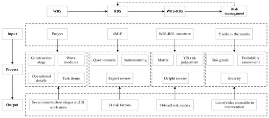
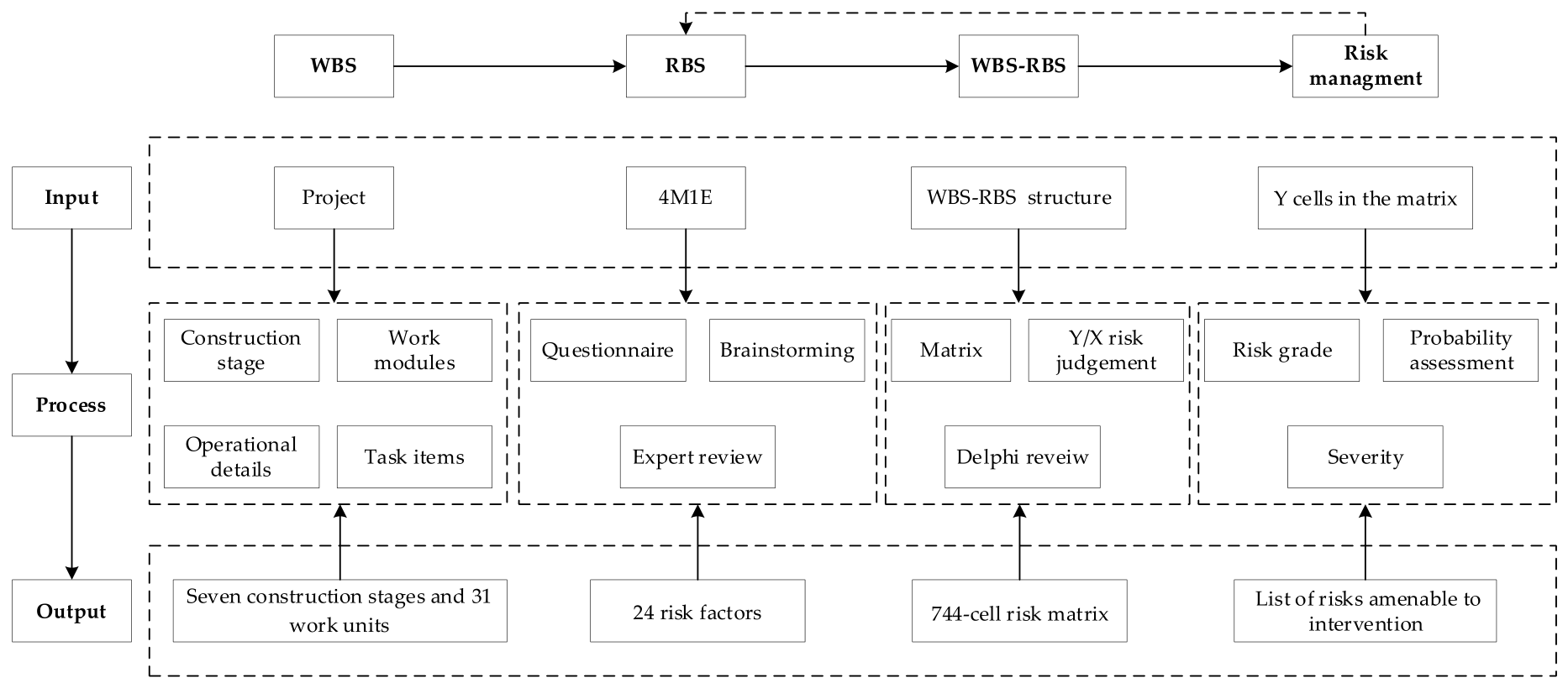
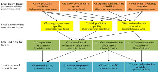
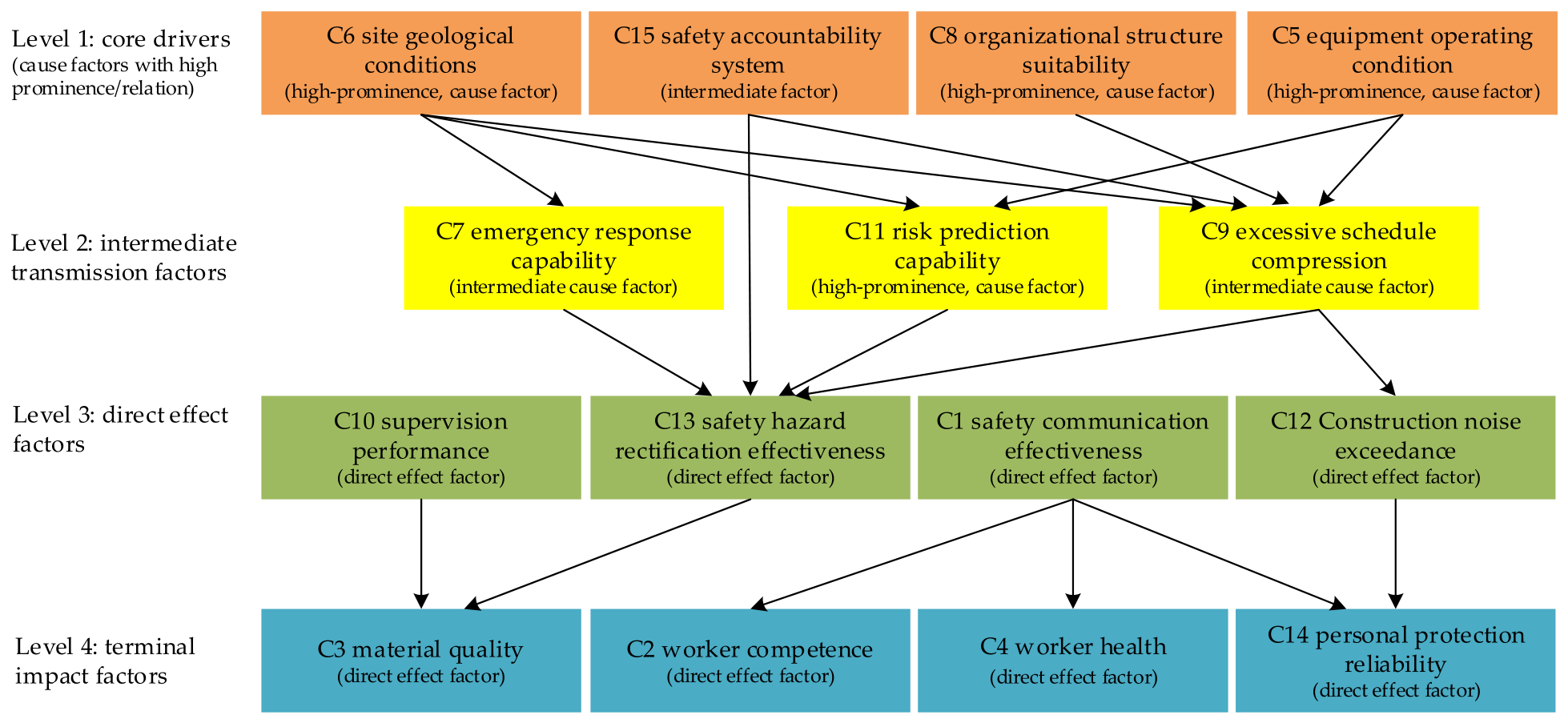
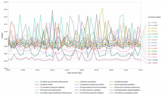
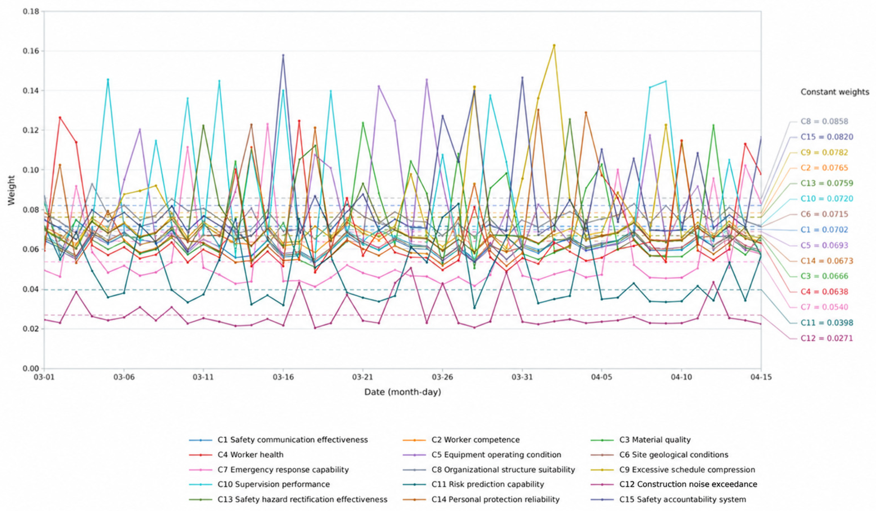
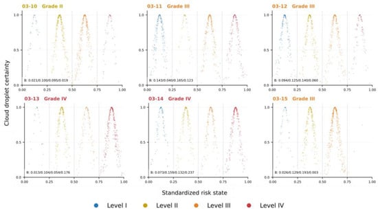
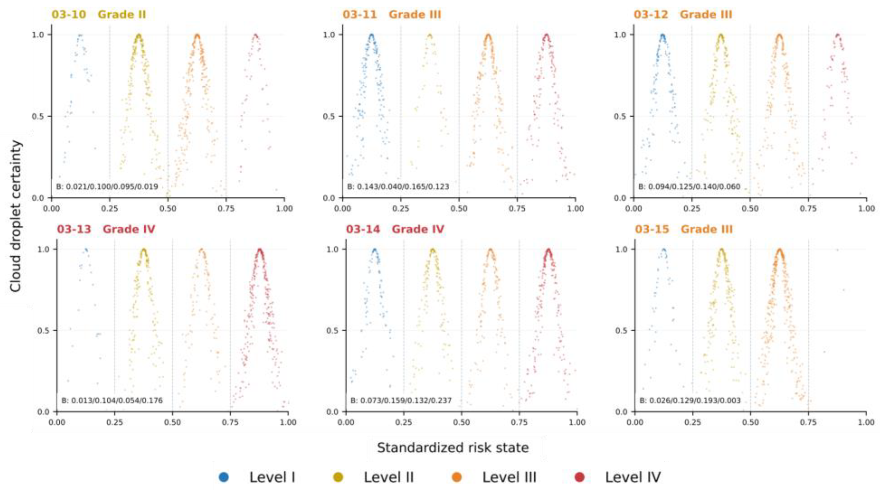
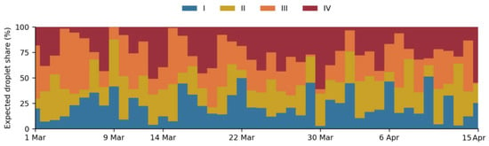
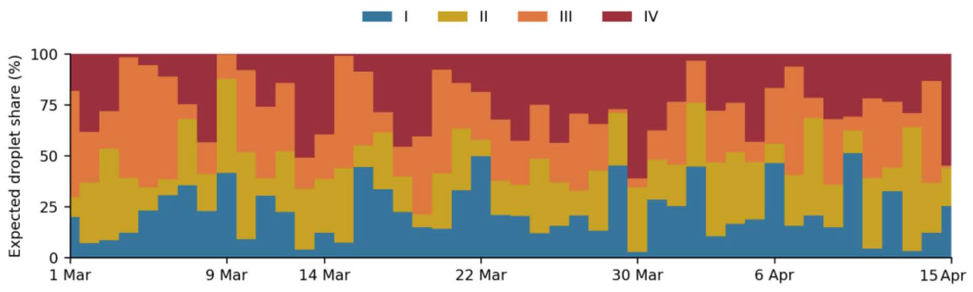
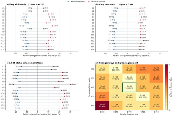
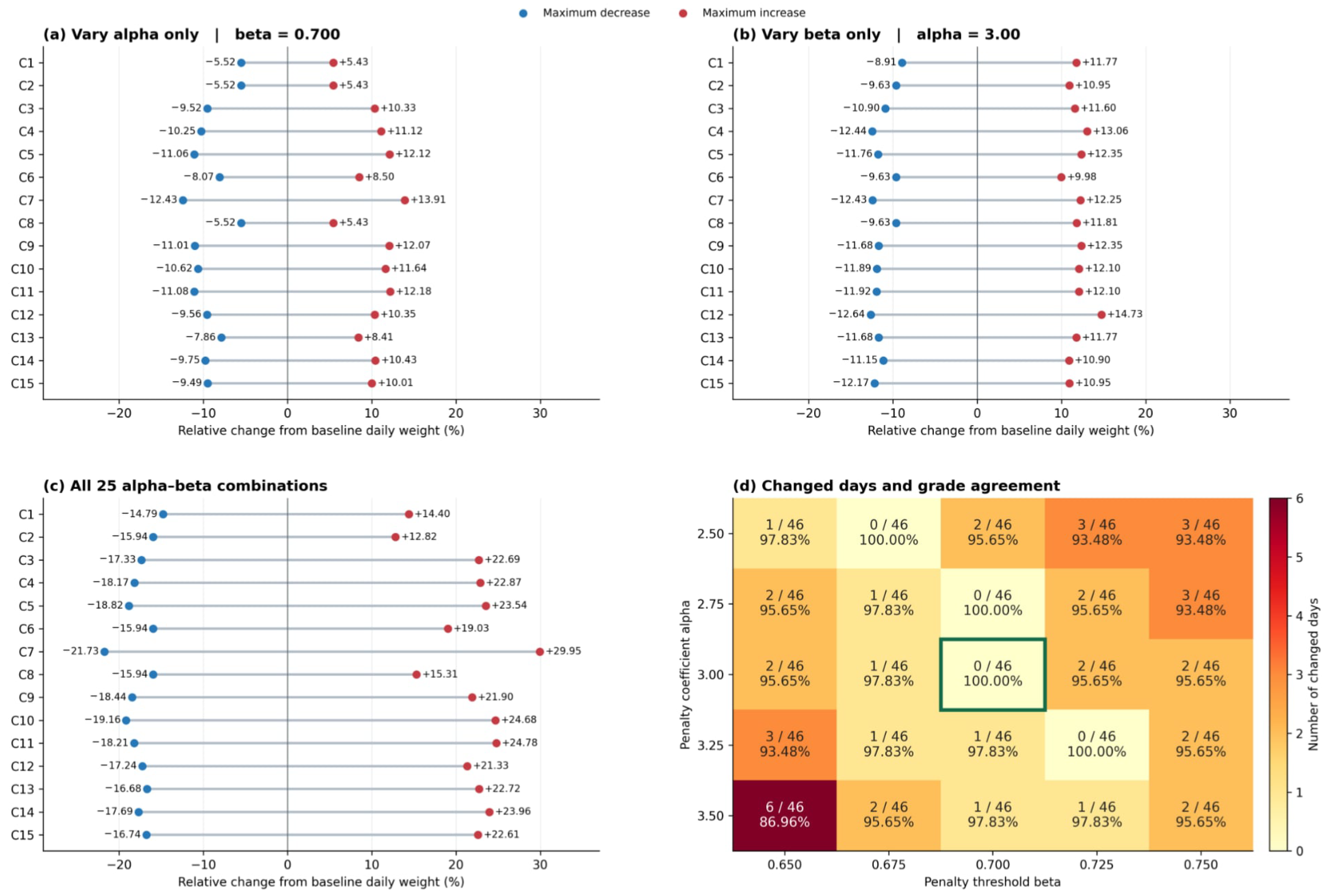

Disclaimer/Publisher’s Note: The statements, opinions and data contained in all publications are solely those of the individual author(s) and contributor(s) and not of MDPI and/or the editor(s). MDPI and/or the editor(s) disclaim responsibility for any injury to people or property resulting from any ideas, methods, instructions or products referred to in the content. |
© 2026 by the authors. Licensee MDPI, Basel, Switzerland. This article is an open access article distributed under the terms and conditions of the Creative Commons Attribution (CC BY) license.