


Abstract
Broadband acceleration peaks can obscure how a storage rack responds at the excitation frequency. This study examines that distinction through shake-table and free-vibration tests on a full-scale, three-level cold-formed steel rack with restrained added mass at its middle level. Six incremental sine-beat runs at nominal 1 Hz were analysed alongside pre-run and post-run impact records. The synchronous top-to-table amplitude ratio remained nearly constant at 2.89–3.04, while the broadband peak ratio increased from 3.43 in the first run to 5.82 in the last. The latter was sensitive to processing bandwidth. Interlevel displacement demand concentrated in the lower two intervals. Free-vibration frequency decreased with response amplitude, and five pre-run impacts reproduced this dependence. A mechanical discussion distinguishes possible geometric and connection-related contributions without assigning a uniquely identified cause. The post-run frequency difference does not establish permanent stiffness degradation. A systematic discrepancy between the acceleration and displacement acquisition chains limits independent validation of absolute laser displacements. These findings support reporting acceleration demand with its processing definition and frequency with its response amplitude.
1. Introduction
Reliable comparison of storage-rack response requires the measured excitation-frequency component to be distinguished from broadband peak demand. Steel storage racks are framed structures assembled from thin-walled cold-formed profiles. They are light in relation to the loads they carry, they reach considerable heights, and they are erected in very large numbers. Their structural behaviour is nevertheless less predictable than that of steel buildings made from standard hot-rolled sections and conventional connections, principally because the uprights are perforated over their full length and because the beam-to-upright and base-plate joints are semi-rigid [1]. The variability of commercial racking systems in components and configurations is such that a design-by-testing approach is commonly adopted [2], and the design provisions themselves differ between Europe and the United States in the member verification procedures and in the admitted analysis approaches [3].
At the component level, the quantities that govern the global response have been measured directly. The rotational stiffness and the moment capacity of the beam-to-upright connection depend on the upright thickness and on the type of tab connector, as shown by flexural tests on 101 assemblies combining three beam sections, three upright thicknesses, and two connector types [4]. Component programmes covering uprights, connections, and base plates have been reported for commercial systems [5]. In a related component study, perforated uprights were characterised in axial compression at three lengths, together with tensile tests on the sheet material, finite-element models, and a comparison against the Effective Width and Direct Strength Methods [6]; that study identified the seismic behaviour of complete rack assemblies as the next step of the programme.
At the scale of the complete rack, the state-of-the-art review of adjustable pallet rack testing for seismic design distinguishes tests on individual components, on subassemblies, on complete racks, and on the stored goods themselves; within the dynamic tests on complete racks, it identifies both variable-frequency sine sweeps and recorded earthquake acceleration signals as established excitation protocols [7]. Static push-over testing has been used to quantify global behaviour in the down-aisle direction, on fully loaded pallet racks within a European research project [1] and on four-level, two-bay commercial racks in a dedicated full-scale facility [2]. Two successive European projects combined component tests with push-over, pseudo-dynamic, and shake-table tests, full-scale sliding tests, and the monitoring of an operating warehouse, and proposed behaviour factors for racking systems [8,9].
Dynamic testing at full scale is less common than static testing, and the campaigns that exist differ widely in specimen, protocol, and instrumentation. Firouzianhaji et al. tested a two-bay, two-level standard cold-formed rack frame on a shake table under El Centro ground motion at low to medium intensities, determined the natural frequency and damping from preliminary tests, and reported that the frames sustained large inelastic deformations without loss of stability [10]. Jacobsen and Tremblay combined quasi-static cyclic tests, pull-back tests, and shake-table tests on cold-formed selective racks; they report drifts of up to 10% without collapse and viscous damping ratios derived from the pull-back records of 2% to 8% for a fixed-base configuration [11]. AL-Gaadi and Alemdar identified the dynamic parameters of three cold-formed rack systems on a shaking table at a scale of 1:3 and reported that the damping ratio varies with the intensity of the excitation [12]. Yılmaz and Alemdar tested a full-scale three-dimensional rack under scaled Northridge records and reported an essentially elastic response up to about half the record intensity, beyond which stiffness degradation and permanent drifts appear, with pallet sliding and connection slip governing the response under strong shaking [13]. Heo et al. examined how the base fixing condition affects the damage and the collapse of a pallet rack on a shake table [14], and Tagliafierro et al. tested a racking structure fitted with curved-surface-slider isolators acting in the cross-aisle direction, reporting a large reduction in the accelerations transmitted to the goods [15].
These studies address different response mechanisms. The inelastic rack-frame response and load mobility examined in [10,11,13] concern response and capacity under earthquake inputs; the base-fixing comparison in [14] addresses the influence of restraint, and the isolation system in [15] modifies the transmission of motion to the goods. Those outcomes cannot be transferred directly to a light shelving module with strapped mass under a fixed-frequency sine beat. The present comparison therefore uses the earlier work to delimit the roles of excitation, restraint, and load mobility, while retaining separate definitions for measured acceleration and displacement demand.
A limit state specific to racking systems is the sliding and the fall of the stored unit loads, which are not mechanically connected to the beams. Shake-table campaigns using several beam finishes report sliding starting at very low acceleration levels in both principal directions [16], and a methodology for estimating sliding displacements has been derived from large sets of response-history analyses [17]. In the campaign reported here, the slabs were strapped to restrain sliding and were treated as fixed added mass in the analysis. Relative load motion was not measured independently; the results are not directly transferable to configurations with freely sliding goods. A comparable distinction separates conventional racks from automated storage systems, whose structural characteristics differ enough from those of ordinary steel buildings for the use of building-code provisions to be questionable [18].
A recent sliding-prediction study [17] addresses movement of unrestrained unit loads, whereas the full-scale earthquake-input study [13] examines sliding and connection effects under stronger shaking. These 2025 and 2026 contributions are relevant context for the present test, but the fixed added mass and harmonic input prevent a direct quantitative comparison of their sliding or inelastic response measures.
Two European standards frame the design of these systems: EN 15512 for structural design [19] and EN 16681 for the principles of seismic design [20].
Two measurement questions motivate the present study. The first is whether a changing ratio of broadband peaks represents a corresponding change in the response synchronous with the excitation; a ratio of separately selected maxima cannot resolve that question on its own. The second is whether a frequency difference between free-vibration records persists when the records are compared at the same response amplitude. The different excitation protocols, load mobility, and boundary conditions of earlier campaigns make those distinctions necessary for comparison; the present work addresses them for one installed rack configuration rather than proposing universal amplification or damage thresholds.
This paper reports a shake-table campaign on a full-scale, three-level cold-formed steel storage rack module carrying a constant added load at a single level. The preceding study [6] examined only the uprights of a rack from the same manufacturer; the present campaign examines the assembled rack. Six runs of incremental harmonic excitation were recorded, with accelerometers and laser displacement transducers at the platen and at each of the three levels, together with free-vibration tests produced by short hammer blows before and after the run sequence. The paper has three objectives. The first is to document the measured broadband acceleration and interlevel displacement response over the six intensities, with the processing chain stated explicitly for every quantity. The second is to separate the response synchronous with the excitation frequency from the broadband peak measures and to quantify how the two evolve with input intensity. The third is to identify the amplitude-dependent dominant longitudinal free-vibration frequency from free vibration and to evaluate the sensitivity of the reported results to the processing choices.
The contribution is the joint assessment of these two interpretation problems using the same installed rack and explicitly defined response measures. Established identification techniques are used to compare nearly constant carrier-frequency response with changing broadband maxima, and within-decay frequency trajectories with differences between test events. This comparison shows which conclusions depend on bandwidth or response amplitude. It provides evidence for interpreting this restrained-load harmonic campaign without claiming a new identification algorithm or a first observation of amplitude-dependent rack dynamics [11,12].
The scope is deliberately narrow. The identification from free vibration is limited to the dominant longitudinal free-vibration frequency and its dependence on amplitude: no damping is estimated, no mode shape is identified, and no inference is drawn about permanent changes in stiffness. The tests do not establish the ultimate capacity of the specimen. No design-code compliance assessment is attempted because the experimental campaign was not conceived as a qualification test and the available information does not fully define the boundary conditions required for such an assessment. What the campaign offers is a transparently processed set of measured responses for a configuration that is common in practice, together with an explicit account of how the numbers would change had they been processed differently.
The full-scale specimen avoids model-to-prototype scaling, and the common carrier frequency permits comparison of synchronous response across intensities. The corresponding limits are the single specimen and mass configuration, the narrow-band input and the absence of repeated tests at each intensity. These are limits on generalisation and repeatability, rather than evidence of a qualification test or of earthquake-spectrum compatibility.
This paper is organised as follows. Section 2 describes the specimen, the loading and support conditions, the instrumentation, the available records, the definition of every response measure and the processing of the free-vibration tests. Section 3 reports the measured response over the six runs, the time histories of the highest run and the frequencies identified from free vibration. Section 4 discusses the sensitivity of the measures to the processing chain, the distribution of the response over the height, the identified frequency and its dependence on amplitude, the relation to previously reported campaigns and the limitations of the study.
2. Materials and Methods
2.1. Test Specimen and Geometry
The specimen was a three-level storage rack module assembled from components of a commercial system produced by SKAT KART SRL, Târgu Secuiesc, Romania. The rack has an overall height of 4495 mm, and each upright frame is 1100 mm deep and is built from two perforated uprights of 85 mm × 52 mm with a wall thickness of 2 mm and a perforation pitch of 50 mm, connected by lacing members of 35.6 × 25 mm and 2 mm thickness; both are of S355J2C steel, and each upright is welded to a base plate of the same steel, 5 mm thick. The beams are closed box sections of 160 × 40 mm formed by welding two C profiles of 158.5 × 40 mm and 1.5 mm thickness in HC340LA steel, and they end in connectors cut from 4 mm plate in S275J2N steel, which engage the perforations of the uprights. The two upright frames are the braced transverse assemblies at the ends of the longitudinal bay. The longitudinal measurement plane is formed by the uprights and beams along one side of the rack depth. Figure 1 shows the geometry, component details and measurement positions. The longitudinal excitation direction is X.
Figure 1.
(a) Rack geometry and schematic measurement positions, with front, side, and top views and component details. (b) Enlarged reference-level diagram distinguishing the overall height of 4495 mm, accelerometer A3 at 4490 mm, and laser point D3 at 4468 mm. The offsets are 5 mm between the top and A3 and 27 mm between the top and D3. The interlevel laser spacings sum to 4468 mm. The inset is schematic and not to scale. Dimensions are in millimetres.
The test specimen was an existing commercial rack module at full scale (1:1), rather than a reduced model designed through similitude relations. Its height, number of levels, member sections and perforation pitch are the properties of the tested product; they were not varied in a parametric programme or optimised for this experiment. No model-to-prototype scaling of geometry, mass, material properties or time was applied. The results consequently describe this commercial configuration and do not establish trends with geometric parameters.
The laser displacement measurement positions were located at the top of the beams, at elevations of 1468, 2968, and 4468 mm above the table reference. These positions define interlevel displacement measurement spacings of 1468, 1500, and 1500 mm. The height H = 4468 mm used to normalise the top-relative displacement refers to D3. The top accelerometer A3 was mounted at 4490 mm, 5 mm below the overall rack height of 4495 mm; its elevation is distinct from the laser measurement elevation. The previous component study [6] examined only the uprights of a rack from the same manufacturer, with nominal section 85 mm × 52 mm and S355MC sheet material. The supplied drawings for the present specimen specify S355J2C; the material measurements in [6] are therefore not used to characterise this specimen.
The principal experimental parameters are summarised in Table 1.
Table 1.
Principal parameters of the experimental configuration.
2.2. Loading and Support Conditions
The added load was placed at the middle level and consisted of five lead slabs of 275 kg each, 1375 kg in total, resting on wooden pallets and secured by straps intended to restrain sliding (Figure 2). The slabs formed two longitudinal rows in the two transverse halves of the 1100 mm depth. The row adjacent to the instrumented longitudinal side contained three equally spaced slabs, 825 kg or 60% of the added lead mass; the opposite row contained two slabs, 550 kg or 40%, staggered longitudinally relative to the three-slab row. The mass configuration was unchanged during the campaign.
Figure 2.
Added load at the middle level: five lead slabs of 275 kg each on wooden pallets of 25 kg each, secured with straps. Three slabs lie on the instrumented side of the rack and two on the opposite side.
The slabs were positioned in two longitudinal rows centred on the axes of the two equal transverse halves of the 1100 mm rack depth. The row centroids are therefore 275 mm on either side of the rack centreline. With 825 kg in the three-slab row and 550 kg in the two-slab row, the transverse eccentricity of the 1375 kg added lead mass is 55 mm towards the three-slab row. This value follows from the confirmed placement and mass distribution; Figure 2 illustrates the arrangement. It refers to the added lead mass.
The rack also carries six wooden pallets of 25 kg each, 150 kg in total, at the first and the second level; those at the second level support the slabs. The added load was transferred through the pallets to the supporting longitudinal beams and through their end connectors to the uprights. Measurements were taken on the longitudinal side adjacent to the three-slab row. The 60/40 split describes the placement of the lead mass; support reactions were not measured, and no 60/40 share of frame reactions is assigned. The specimen was mounted on the shake-table platen through the base plates described above. The number, diameter, and tightening of the anchors, and the detail of the connection between base plate and platen, are not documented in the material available for this campaign. Neither the restraint stiffness nor possible local slip is therefore known, and the response is described for the loaded rack assembly as installed on the shake table, including the actual base restraint, without assuming perfectly rigid base connections. The reported frequencies characterise this installed configuration; the measurements do not identify the dynamics of the platform separately.
2.3. Instrumentation and Data Acquisition
Four triaxial wireless accelerometers, G-LINK-200-8G (Parker LORD MicroStrain, Williston, VT, USA), were recorded through a WSDA-200-USB gateway (Parker LORD MicroStrain, Williston, VT, USA). Four optoNCDT ILR 2250 laser displacement sensors (Micro-Epsilon, Ortenburg, Germany) were recorded through a four-channel IF2004/USB converter (Micro-Epsilon, Ortenburg, Germany). A0–A3 denote the accelerometers and D0–D3 the displacement measurement points on the table and at the three rack levels. Figure 3 shows the acquisition chains; the channel assignments are given in Table 2.
Figure 3.
Experimental configuration, instrumentation, and data-acquisition chains. The photograph identifies the table and three measurement levels and shows the added mass at the middle level. A0–A3 denote triaxial accelerometers; D0–D3 identify the displacement measurement points. Acceleration and displacement channels are recorded through separate acquisition chains. The software screenshots illustrate the acquisition interfaces. The ±8 g label denotes the sensor model’s nominal capability; the acquisition range used in the tests was ±2 g.
Table 2.
Instrumentation, channel assignment and laser measurement elevations. The top accelerometer A3 is at 4490 mm; the laser elevation at D3 is 4468 mm.
The accelerometers were manufactured in 2023 and had manufacturer calibration certificates. The acquisition range was set to ±2 g during the March 2024 tests.
The acceleration records were sampled at 256 Hz. In the record used for the response quantities reported here, all twelve channels are complete, with no missing values and no discontinuity in the time vector. The unit g is adopted from the experimental documentation and is supported by the means of the vertical channels, which lie close to ±1; the export header does not populate the unit fields. The sensor model has a nominal ±8 g measurement capability and a configurable input range. The acquisition range was set to ±2 g. The internal low-pass and high-pass filter settings were not recovered for the retrospective analysis.
The longitudinal channel assignments are given in Table 2. The vertical axes were checked against the static gravitational component: over the first 30 s of both records, their means were close to ±1 g, whereas the means of the selected longitudinal channels were below 0.016 g. Principal-component analysis of the horizontal channels in the 0.5–2 Hz band supported the selected longitudinal direction.
The sign conventions of the four units are not identical. During free vibration, when all three levels move with closely aligned longitudinal responses, the records of A2 and A3 are anti-correlated with those of A1 and A0, with correlation coefficients between −0.991 and −0.999 over six separate free-decay events. The same anti-correlation appears during the runs. A2 and A3 therefore measure with the opposite sign to A1 and A0, and their records are inverted before any operation that combines channels. Peak magnitudes are unaffected by this correction; signed histories, pointwise differences and phases are not.
The laser acquisition applied a moving median over 8 samples and delivered an output every 48 ms, with individual distance offsets per sensor and error codes replaced by zero. The sampling rate upstream of the time-based subsampling is not documented, so the duration of the median window cannot be stated from the header alone.
D0 records the motion of the shake-table platen at the reference elevation. Positions A1–A3 and D1–D3 identify the instrumented rack levels in Figure 1. The displacement elevations measured during assembly are used to normalise the interlevel and top-relative displacements. Acceleration profiles are plotted by measurement level.
2.4. Available Records and Excitation
The response quantities reported here are taken from the record of 29 March 2024, which spans 09:27:57.504 to 09:42:33.859 UTC with 224 348 samples per channel and contains all six dynamic runs. A second record, from 28 March 2024, contains 27 time discontinuities of up to 920 s and unequal numbers of missing values between nodes; it is therefore not used for the dynamic runs. Its continuous segments are used in Section 2.7 for the free-vibration tests, where every analysis window was checked for continuity of the sample stream before being retained.
Six dynamic runs were identified in the 29 March record. Segmentation was performed on the root-mean-square value of the candidate table channel in the 0.5–2 Hz band, and the count of six is unchanged at detection thresholds of 0.008, 0.010, and 0.015 g. At the 0.010 g threshold, the active intervals begin at 11:30:48, 11:35:50, 11:36:44, 11:37:48, 11:39:00, and 11:40:33 local time and last between 17.9 and 21.2 s. These durations are defined by the detection threshold and represent neither the commanded duration of the platform motion nor the subsequent free response; the analysis windows used for the peak values were longer than the active intervals.
The campaign comprised ten actions. The present analysis is restricted to the six dynamic runs contained in the selected record, labelled Run 1–Run 6 in chronological order.
The six-run sequence was stopped after Run 6 because the large observed displacements did not permit safe continuation, as confirmed by the experimenter. The run count therefore reflects an operational safety decision, rather than a statistically selected sample size or attainment of a demonstrated ultimate capacity. The available continuous record contains these six dynamic runs; the incomplete account of the other campaign actions remains a limitation.
The excitation was a sine-beat signal with a nominal frequency of 1 Hz. The carrier frequency used for the synchronous analysis was estimated separately for each run as described in Section 2.5 and ranged from 1.0072 to 1.0078 Hz.
The applied input is the acceleration recorded directly on the platen by calibrated accelerometer A0. The reported input quantities therefore describe the measured platform motion and do not assume exact reproduction of the nominal command.
The experimenter selected a nominal frequency of 1 Hz with the intention of obtaining a large, amplified response in the vicinity of the longitudinal resonance. This was a fixed-frequency harmonic loading choice, not a resonance-tracking procedure: the measured carrier frequencies remain below the free-vibration frequencies reported for the tested states. The changing beat envelope allows the carrier-frequency response to be examined, but the signal is not presented as a spectrum-compatible earthquake record.
2.5. Signal Processing and Definition of the Response Measures
The longitudinal acceleration records were processed using a symmetric finite impulse response filter with 257 coefficients, a Hamming window, and a cut-off frequency of 25 Hz at a sampling rate of 256 Hz. Centred convolution was applied to the complete record, with constant extension of 128 samples at each end. The analysis windows were then extracted, and each channel’s window mean was removed before calculating peaks or relative acceleration histories.
Let (t) denote the processed longitudinal acceleration and (t) the displacement at measurement position i, with i = 0 at the table. The peak acceleration is , and the top-to-table peak ratio is . The peak displacement is , the peak displacement relative to the table is , and the peak interlevel displacement is . Signed histories retain positive and negative values; “absolute acceleration” distinguishes the individual measured acceleration from acceleration relative to the table.
R compares two independently determined peaks that generally occur at different instants; it is not a transfer function or an identified modal amplification factor. Relative acceleration and displacement histories are obtained by pointwise subtraction of channels recorded within the same acquisition system. Their peaks are not calculated by subtracting independently selected channel peaks.
A second, narrow-band measure is used alongside R. The excitation frequency of each run is estimated on the table channel by least squares over a fine frequency grid. For each channel, the complex demodulated envelope and the synchronous amplitude and phase are defined as
The low-pass operation is a centred, unit-sum Hann smoothing kernel spanning 3.0 s (768 samples at 256 Hz), corresponding to approximately three carrier cycles. Samples for which the complete centred kernel is unavailable are excluded from the envelope-maximum search. The three-second duration suppresses the twice-carrier term while retaining the slowly varying sine-beat envelope. The four channels are read at the instant at which the table envelope is largest. The synchronous response ratio is = / and the phase lag is − . Repeating the calculation with 2 s and 4 s Hann kernels gives top-to-table ratios between 2.87 and 3.05, compared with 2.89 to 3.04 for the 3 s reference, so the conclusion is insensitive to this choice over the tested range.
The interlevel displacement ratios are 100/, with = 1468 mm and = = 1500 mm. The top-relative ratio is 100/H, with H = 4468 mm. The first measurement spacing is smaller than the upper spacings. Consequently, the interval with the largest displacement in millimetres need not have the largest ratio.
The displacement histories were regenerated from the original laser export. The zero reference is the median of each channel over the first 30 s of acquisition. Values with an absolute magnitude exceeding 300 mm were flagged; no flagged or interpolated samples occur within the six analysis windows. The windows start at 11:30:45, 11:35:47, 11:36:41, 11:37:45, 11:38:57, and 11:40:30 local time and have durations of 26, 28, 28, 29, 29, and 29 s, respectively, with inclusive endpoints. The reported displacement peaks retain this initial reference rather than a separate zero before each run.
2.6. Synchronisation, Data Quality, and Uncertainty
The two acquisition systems write different time bases: the accelerometer export is in UTC, the laser export in local time. After adding two hours to the acceleration time vector, a residual offset remains. It was quantified by cross-correlating the table acceleration with the negative of the table displacement, both band-limited to 0.7–1.3 Hz, over 17 s intervals within each run, searching lags between −0.45 and +0.45 s. The correlation coefficient after shifting is 0.999 or better in all six runs, against −0.27 to −0.34 at zero lag, and the lag that maximises it increases slightly from 0.291 s in Run 1 to 0.304 s in Run 6.
This result is treated as a diagnostic of the combined acquisition chains, including transducer response, filtering, and clocks. It does not isolate a clock error, it does not establish a final synchronisation rule, and the 1 ms search step does not represent a physical precision of 1 ms. Because the signal is nearly periodic, alternative solutions at larger lags cannot be excluded on the basis of correlation alone; closing this point requires start and stop events or individual sensor time stamps. The offset is a property of the relation between the two systems and is not applied to differences between channels acquired by the same system.
Samples exceeding a diagnostic threshold of 300 mm in absolute value were examined in the laser record: 2443 consecutive samples on channel d2 between 11:41:37.885 and 11:43:35.207, two sequences of 8 and 15 samples on d3, one of 32 samples on d4, and none on d1. All occur after the six runs. The threshold is an inspection criterion, not a complete interpretation of the transducer error codes.
Processing sensitivity was assessed by changing the FIR cut-off to 20 or 30 Hz, shifting the analysis-window bounds by ±0.3 s, and changing the displacement reference to the first 10 or 60 s or to the 5 s preceding each window. These alternatives describe processing sensitivity, not confidence intervals. The principal bandwidth and baseline effects are presented in Supplementary Figures S1 and S2. The exported displacement increment is 0.1 mm; this increment is not a calibration uncertainty.
The internal sensor filter settings were not recovered. Their effect is distinct from the documented sensitivity to the 20–30 Hz software-filter cut-off: refiltering an exported record cannot restore information removed before export. The laser records have moving-median preprocessing, a coarser output interval, and a residual inter-system time offset, so they cannot independently validate the high-frequency acceleration content. The filter comparison quantifies sensitivity to the stated software-processing choices; it does not reconstruct the internal sensor filtering.
A separate acceleration–displacement check compares carrier-frequency amplitudes using the same centred 3 s Hann demodulation and each acquisition chain’s own table-envelope maximum. Only for this diagnostic, the laser histories are linearly interpolated to 256 Hz; the reported laser peaks are unchanged. No inter-system phase is evaluated. Table S3 compares laser amplitudes with displacement-equivalent acceleration amplitudes at the measured excitation frequency. The laser/equivalent-displacement ratios are 0.788–0.840 across the six runs and four positions. The upstream laser sampling rate and the resulting transfer characteristics of the eight-sample median are not recovered, so the difference cannot be assigned a unique source or corrected from the available metadata.
Additional checks use the unfiltered acquisition exports, meaning the recorded sensor outputs before the present software FIR. Across all twelve axes of the dynamic record, the largest absolute exported value is 1.313 g; no value reaches 1.99 g, and each channel extreme occurs without a multi-sample plateau. These observations show no clipping signature in the available export but cannot establish the absence of distortion before export. Table S1 lists the extrema; Table S2 and Figure S6 compare A0 and A3 at 20, 25, and 30 Hz and show same-window spectra for Runs 2 and 6.
2.7. Free-Vibration Tests and Spectral Processing
A second acceleration record, from the same four triaxial units and at the same sampling rate of 256 Hz, covers 28 March 2024 from 10:47:48 to 12:55:42 local time. That session was used to erect and instrument the specimen, to place the added mass and to determine its dynamic characteristics: free vibration was induced by short blows of a rubber hammer applied in the longitudinal direction. The 29 March record analysed in Section 3.1, Section 3.2, Section 3.3, Section 3.4 and Section 3.5 contains one further blow of the same kind, applied with the table at rest about forty seconds after the end of the sixth run.
The acquisition dates distinguish the pre-run free-vibration session from the session containing the dynamic runs and the single post-run event. This separation is retained because the pre/post comparison was not performed within one uninterrupted test session. Dates are not used as explanatory variables; they document a condition that limits attribution of the observed frequency difference to the dynamic sequence.
Candidate events were located from the envelope of the processed top-level longitudinal channel and retained only when three conditions were met: the peak table acceleration over the analysis window remained below 0.002 g, so that the record is free vibration and not a response to residual table motion; the sample stream was continuous over the window; and no further blow occurred within it. Twelve candidate events were found in the 28 March record. Two were rejected because the record is discontinuous within the window, and four, applied between 10:55 and 10:58, because successive blows are less than 45 s apart. Of the six that remain, one was applied at 11:03:31, while the added mass was still being placed; the loading state at that instant is not documented, and that event is reported separately. Five events with the full added mass in place, together with the single event of 29 March, form the set analysed here.
The records were filtered with the same 25 Hz finite impulse response filter described in Section 2.5. Two windows were taken from each event, both measured from the instant of the peak: a 6 s window covering the first cycles of the decay, and a 20 s window starting 15 s after the peak, by which time the response has fallen by one to two orders of magnitude. A third window of 20 s, beginning at the peak itself and therefore covering both the high-amplitude start of the decay and its tail, is used for the free-vibration spectra reported in Section 3.6, for the transverse peak reported in Section 3.6 and for the distribution of spectral amplitude over the height in Section 3.6. Each window was detrended by its mean, tapered with a Hann window and transformed with zero padding, and the longitudinal peak was read in the band 0.6 to 4.0 Hz. The transverse peak was read separately from 3.5 to 5.5 Hz. Zero padding refines the evaluation grid and not the physical resolution, which is 0.17 Hz for the 6 s window and 0.05 Hz for the 20 s window. For the long windows, the peak frequency was also estimated by counting the zero crossings of the same signal after a 3 Hz low-pass filter using the same 257-coefficient Hamming FIR construction and centred convolution; for these 20 s low-amplitude windows, the two estimators agree to within 0.003 Hz in every event. Fourier peaks are used for the spectra and for the long windows, but not for the dependence of the frequency on amplitude: over a 6 s window the physical resolution is 0.17 Hz, which zero padding refines only as an evaluation grid. For that purpose, each 6 s window, low-passed using the same 3 Hz FIR, is instead fitted by least squares with a damped sinusoid, c + exp(−t)(a cos 2πft + b sin 2πft), the two nonlinear parameters being obtained by a grid search and refined, and the linear parameters by ordinary least squares. The successive windows of one event advance by 3 s and therefore overlap by 50%, so the points of a single decay are not independent observations and are shown as a trajectory. The formal standard error of f from the fit covariance is below 0.001 Hz, which understates the true uncertainty because the noise is correlated by the filter; the reproducibility across the five separate pre-run impact events compared at matched response amplitude, a pooled standard deviation of 0.011 Hz, is the figure used here. The decay rate is a nuisance parameter of the fit and is not reported as a damping ratio. No damping ratio is estimated, and no mode shape is identified. The quantities reported are peak frequencies of measured spectra, their dependence on the amplitude of the window, and the distribution of spectral amplitude at those frequencies over the height. For comparisons at matched response amplitudes, frequency was interpolated linearly with respect to log10(a3) between adjacent points of each decay trajectory; the pre-run reference at each target amplitude is the mean of the five interpolated M1–M5 values. Anthropic Claude (Claude Opus 5.5, Medium setting) and OpenAI Codex (GPT-6.1 Sol, Medium setting) assisted with data-processing tasks and preparation and checking of analysis scripts. All processing choices, methods, numerical results and interpretations were reviewed and verified by the authors. The tools were not used to generate scientific conclusions independently.
3. Results
3.1. Input Intensities and Recorded Sequence
Six dynamic runs are present in the record analysed here. The peak longitudinal acceleration measured on the shake-table platen increases from run to run, from 0.068 g in the first run to 0.178 g in the sixth, the intermediate values being 0.093, 0.116, 0.121, and 0.157 g. The increment between the third and the fourth run is the smallest of the sequence, 0.005 g, so the six runs do not form a uniformly spaced series of intensities. The active interval of each run, defined by the detection threshold, lasts between 17.9 and 21.2 s. Figure 4 shows the complete table record, the analysis windows and the detected active intervals.
Figure 4.
Recorded platen input: (a) complete acceleration record and the six analysis windows; (b) enlarged Run 6 history at A0, with all recorded samples retained. Shaded regions in (a) indicate the analysis windows; the active intervals use the 0.010 g RMS threshold in the 0.5–2 Hz band. Panel (b) uses the same 25 Hz FIR filtering and window-mean removal as Table 3. Time zero in (b) is 11:40:30 local time on 29 March 2024. The measured platen peak in Run 6 is 0.178 g. The plotted motion is the measured input, not an idealised or commanded waveform.
The acceleration trace is filtered using the 257-coefficient Hamming-window FIR filter with a 25 Hz cut-off. Emphasised window traces have their respective window means removed; the background trace has its full-record mean removed and is displayed using peak-preserving minimum/maximum pairs over 0.25 s bins. Time is measured from the start of the acceleration record; 1 g = 9.80665 m/s2.
The peak table displacement follows the same ordering, from 5.3 mm to 28.6 mm. All values reported in this section refer to the longitudinal direction.
3.2. Longitudinal Acceleration Peaks and Top-to-Table Peak Ratios
Table 3 gives the peak absolute acceleration at the four instrumented positions for each run, together with the top-to-table peak ratio R. At the top level, the peak rises from 0.235 g to 1.034 g, that is, by a factor of 4.4, while the table input rises by a factor of 2.6 over the same sequence. Figure 5 compares the distribution of these independently determined peaks over the measurement levels.
Table 3.
Peak longitudinal accelerations and top-to-table peak ratios for the six runs.
Figure 5.
Peak longitudinal accelerations at the table and the three rack levels for Runs 1–6. Peaks are the maximum absolute values after 25 Hz FIR filtering and removal of the mean of each analysis window. Lines connect measurement levels for visual comparison; the peaks need not occur simultaneously, and the profiles do not represent mode shapes. 1 g = 9.80665 m/s2.
The distribution of the peaks over the height is not monotonic in every run. In the first four runs, the peak recorded at Level 1 exceeds the peak recorded at Level 2: 0.190 g against 0.116 g in Run 1 and 0.252 g against 0.223 g in Run 4. In the last two runs, the ordering is reversed, with 0.307 g against 0.304 g in Run 5 and 0.481 g against 0.428 g in Run 6. The top level carries the largest peak in every run.
Figure 6 shows the top-to-table peak ratio as a function of the measured input intensity. For the reference 25 Hz processing, R increases from 3.43 in Run 1 to 5.82 in Run 6, with an initial decrease to 3.25 in Run 2. The sequence depends on the filter bandwidth: in Run 2, R is 4.97 at 20 Hz and 2.63 at 30 Hz, compared with 3.25 at 25 Hz. Figure S1 shows the full comparison. The six peak ratios are therefore interpreted as processing-defined response measures, without fitting a constitutive relation or assigning a modal mechanism.
Figure 6.
Top-to-table peak acceleration ratio, R, versus peak table acceleration for the six runs. R is the ratio of independently determined top and table peaks, both evaluated after 25 Hz FIR filtering and window-mean removal. The numerical labels 1–6 identify Runs 1–6, respectively; the connecting line indicates their chronological order. R is a descriptive peak ratio, and its filter-bandwidth sensitivity is shown in Figure S1.
3.3. Response at the Excitation Frequency
The peak ratio R compares two maxima that occur at different instants and over the full retained bandwidth. A second measure was therefore extracted at the frequency of the applied excitation, using the complex demodulation defined in Section 2.5. For each run, the carrier frequency estimated on the table channel is 1.0072 to 1.0078 Hz. The synchronous amplitudes and phases are read for all four channels at the instant at which the table envelope is largest, so the values refer to the same instant of the beat. Table 4 lists the results for the six runs.
Table 4.
Synchronous response at the excitation frequency.
The synchronous amplitude at the top level grows approximately in proportion to the synchronous amplitude at the table over the whole sequence, from 0.079 g to 0.442 g, while the table grows from 0.027 g to 0.153 g. is 2.95 on average, with values between 2.89 and 3.04 and a standard deviation of 0.07 over the six runs. The ratios at the lower levels are similarly stable, 1.76 to 1.84 at Level 1 and 2.41 to 2.51 at Level 2. The reported top-level phase difference is −1.9° to −4.8°, so the top response is nearly in phase with and slightly lags the table. Over the same six runs, the broadband peak ratio R grows from 3.43 to 5.82. Figure 7b places the two measures side by side.
Figure 7.
Response at the excitation frequency: (a) synchronous top amplitude against synchronous table amplitude, with the reference line = 2.95, corresponding to the mean of the six synchronous ratios; (b) the synchronous ratio and the broadband peak ratio R against the peak table acceleration.
3.4. Absolute, Relative and Interlevel Displacements
Table 5 gives the peak absolute displacements at the four positions, the peak relative displacement of the top level with respect to the table, and the peak interlevel displacements, together with the corresponding ratios. The peak absolute displacement of the top level increases from 14.3 mm to 86.6 mm, and the peak relative displacement from 9.2 mm to 61.3 mm, that is, from 0.206% to 1.372% of the elevation of the top transducer. Figure 8 represents the top-relative displacement using equivalent millimetre and percentage scales; Figure 9 compares the three interlevel responses.
Table 5.
Peak displacements, relative displacements, and interlevel displacements for the six runs.
Figure 8.
Peak top displacement relative to the table versus peak table acceleration.
Figure 9.
Interlevel displacement response versus peak table acceleration: (a) peak interlevel displacements; (b) the corresponding displacement ratios. Each interlevel peak is the maximum absolute difference between adjacent displacement histories. Ratios use h1 = 1468 mm and h2 = h3 = 1500 mm. Displacements retain the reference established over the first 30 s; acceleration peaks use the 25 Hz FIR filter and window-mean removal. The close ordering of the first two ratios in Run 3 depends on the displacement reference (Figure S2).
In Run 6, the peak interlevel displacements are 24.7, 27.1, and 19.6 mm at the first, second and third levels. Their sum, 71.4 mm, exceeds the peak relative displacement of the top level, 61.3 mm, because the three maxima do not occur at the same instant; this is a direct consequence of the definitions in Section 2.5 and not an inconsistency in the measurements.
Expressed as ratios of the measured transducer spacings, the same run gives 1.683%, 1.807%, and 1.307%. The level carrying the largest value in millimetres and the level carrying the largest ratio coincide in five of the six runs. They differ in Run 3, where the largest interlevel displacement in millimetres occurs at the second level, 8.6 mm, while the largest ratio occurs at the first level, 0.579%, because the first spacing is smaller than the other two. The two quantities are therefore reported separately throughout.
For the initial 30 s reference, the largest interlevel ratio occurs in interval 0–1 in Runs 1–3 and in interval 1–2 in Runs 4–6. The Run 3 ratios are close: 0.579% and 0.573% for the first two intervals. Their ordering reverses when the reference is taken over the first 60 s or immediately before the run. Figure S2 shows this sensitivity. The lower-intensity Runs 1–2 and higher-intensity Runs 4–6 retain their respective dominant intervals in the tested baseline alternatives; the exact transition at Run 3 is not treated as robust.
The relative peak is calculated as the maximum absolute difference between the D3 and D0 time histories, using the displacement reference established over the first 30 s of the record. The secondary axis expresses the same quantity as a percentage of H = 4468 mm, the elevation of the upper displacement measurement point. Table acceleration peaks are evaluated after 25 Hz FIR filtering and window-mean removal. Sensitivity to the displacement reference is shown in Figure S2.
3.5. Time Histories of Run 6
Run 6 is the sixth analysed window, beginning at 11:40:30 local time. Figure 10 superposes the signed accelerations at A0–A3, with the table reference A0 shown in red. Figure S3 shows the pointwise relative acceleration of the top level with respect to the table, formed after the polarity correction of Section 2.3. Its maximum absolute value is 0.940 g at 16.098 s from the window start. Without that correction, the same operation returns 1.128 g, because it then adds two signals of opposite sign instead of subtracting them. This differs from the difference in the individual acceleration peaks because the channel values must be compared at the same instant.
Figure 10.
Superposed signed longitudinal acceleration histories at A0–A3 during Run 6. The records use the 25 Hz FIR filter and removal of each channel’s analysis-window mean. A0 is shown in red in the foreground. Absolute denotes the measured acceleration at each position, not the absolute value of the signal. Time zero is 11:40:30 local time on 29 March 2024; 1 g = 9.80665 m/s2.
Figure S4 superposes D0–D3, with the table reference D0 shown in burgundy. The histories retain the acquisition-record zero reference. The median top-to-table offset over the 5 s preceding Run 6 is +3.9 mm; removing the per-channel pre-run offsets changes the top-relative peak from 61.3 to 57.4 mm. This illustrates a change in reference and does not independently establish structural residual deformation. Figure 11 shows the signed interlevel differences. Their maxima reproduce the values in Table 5. No cross-system alignment is applied to these separate acceleration and displacement plots.
Figure 11.
Signed interlevel relative displacement histories during Run 6, calculated point by point as D1–D0, D2–D1, and D3–D2. The displacement reference is the same as in Figure S4. The maximum absolute interlevel displacements are 24.7, 27.1, and 19.6 mm, respectively, and need not occur simultaneously. Time zero is 11:40:30 local time.
3.6. Spectral and Free-Decay Observations
Six free-vibration events satisfy the conditions of Section 2.7: five recorded on 28 March with the full added mass in place and before any dynamic run, and one recorded on 29 March, after the sixth run. Table 6 lists them. Figure 12a shows the longitudinal acceleration at Level 3 during the thirty seconds that follow the largest blow, and Figure 12b the corresponding amplitude spectra. The table channel stays below 0.001 g throughout every window, so each record is free vibration of the specimen and not a response to table motion.
Table 6.
Free-vibration events retained for spectral analysis. The longitudinal frequencies in the high- and low-amplitude windows are Fourier peak estimates; the zero-crossing estimate is reported separately. The transverse peak is searched in the 3.5–5.5 Hz band.
Figure 12.
Free vibration after a hammer blow: (a) longitudinal acceleration at Level 3 during the 30 s following the largest blow, event M2; (b) normalised amplitude spectra for four representative events, calculated from the 20 s window beginning at the blow, which is not the low-amplitude window of Table 6, and normalised to the maximum in the 0.6–4.0 Hz band. The four curves span the pre-run amplitude range and include the post-run event; all six retained events are used in the quantitative results.
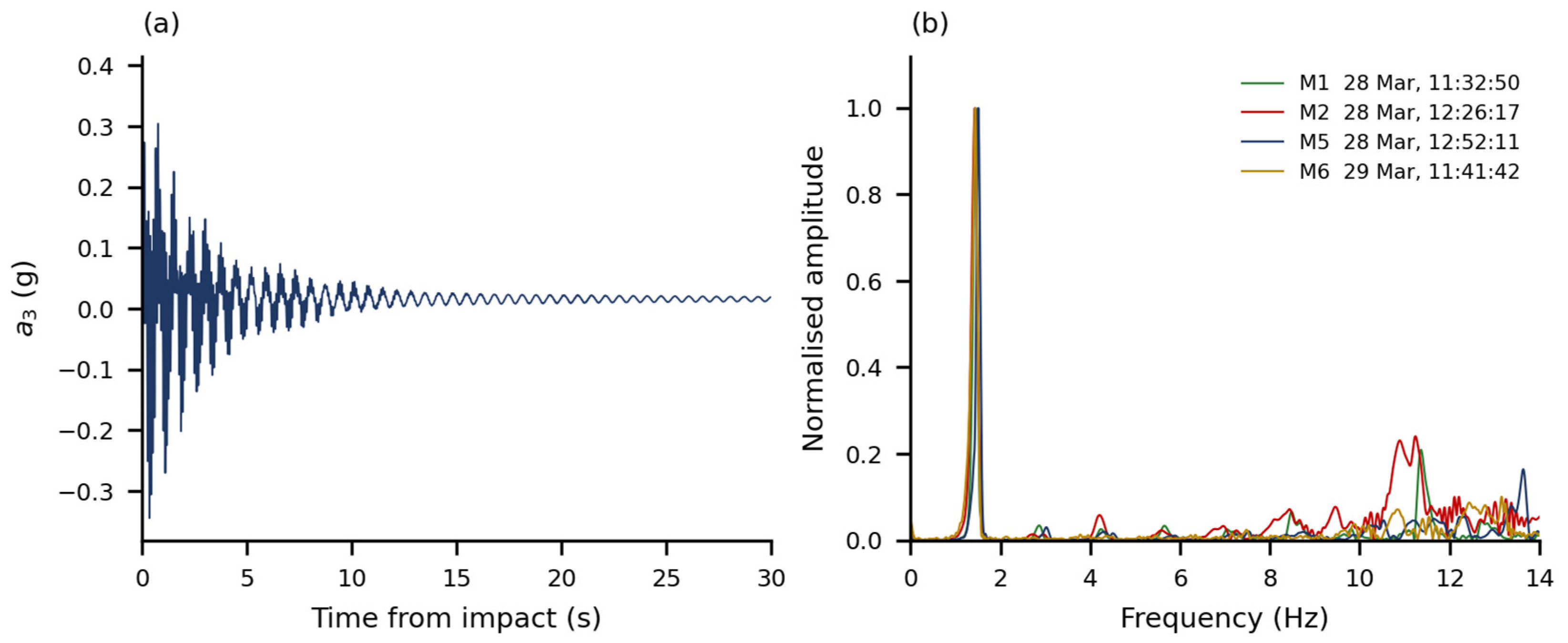
In the five events of 28 March, the peak frequency of the low-amplitude window lies between 1.512 and 1.529 Hz, with a mean of 1.520 Hz and a total spread of 0.018 Hz. The zero-crossing estimate of the same windows gives 1.511 to 1.532 Hz. In the 29 March event, the low-amplitude window gives 1.486 Hz and the zero-crossing estimate 1.485 Hz.
The identified frequency depends on the amplitude of the window from which it is read. Within the largest decay, it rises from 1.344 Hz in the first 6 s, where the peak response is 0.362 g, to 1.510 Hz eighteen seconds later, where the peak response is 0.0078 g, an increase of 12%. Table 7 gives the complete sequence for that event and for the event of 29 March, and Figure 13 plots all six events. The five events of 28 March follow one another closely although their initial amplitudes differ by a factor of four and a half, and they were not applied in order of increasing amplitude; compared at matched amplitude, they agree to a standard deviation of 0.011 Hz.
Table 7.
Identified frequency and peak response amplitude in successive 6 s windows of two free-vibration events, from the damped-sinusoid fit of Section 2.7.
Figure 13.
Identified frequency of the longitudinal channel at Level 3 against the peak response amplitude of the same window, for successive 6 s windows of each free-vibration event. The five events of 28 March precede the run sequence; the event of 29 March follows it. Successive windows of one event overlap by 50%, so each event is a trajectory and not a set of independent observations. The bar shows the inter-event reproducibility at matched amplitude, 0.011 Hz; the formal covariance standard error of the fit, below 0.001 Hz, does not represent the correlated-noise uncertainty and is not plotted.
The track of the 29 March event lies below the 28 March band over the whole amplitude range in which both are defined. Compared at equal response amplitude, the difference is 0.080 Hz at 0.005 g, 0.095 Hz at 0.010 g, 0.107 Hz at 0.020 g, and 0.112 Hz at 0.050 g, that is, 5.2% to 7.8%. Compared instead between the decayed tails of the two sets, without matching the amplitude, the difference is 1.520 Hz against 1.486 Hz, or 2.2%. Both figures describe the same pair of records; they differ because the tails are reached at different amplitudes.
Two further loading configurations of the specimen were characterised by the same impact method during assembly, on the same longitudinal channel at Level 3. The dominant longitudinal free-vibration frequency is 6.00 Hz for the bare frame and 3.87 Hz once the wooden pallets are in place. The records of those two tests are not among those re-analysed here, so the two values are reported as obtained and are not accompanied by a window or a response amplitude. The earliest data in the 28 March record already show a longitudinal frequency of about 1.7 Hz, the ambient windows between 10:51 and 10:55 giving 1.61 to 1.76 Hz, so part of the added load was in place before the recording began. Table 8 collects the three loading configurations and the post-run state of the fully loaded configuration; Figure 14 shows the progression.
Table 8.
Dominant longitudinal free-vibration frequency for three loading configurations and the post-run state of the fully loaded configuration.
Figure 14.
Dominant longitudinal free-vibration frequency for three loading configurations and the post-run state of the fully loaded configuration, with the amplitude-dependent range shown for the fully loaded states. The values for the bare frame and for the frame with pallets were obtained during assembly, and their response amplitude is not documented.
The single event recorded at 11:03:31 on 28 March, while the added mass was still being placed, gives 1.492 Hz in the 6 s window at a peak response of 0.089 g and 1.608 Hz in the low-amplitude window, against 1.605 Hz by zero crossings. It is quoted here for completeness and is not used in any comparison, because the mass present at that instant is not documented.
The transverse channel of the same unit shows a peak between 4.20 and 4.44 Hz in every event, at amplitudes an order of magnitude below the longitudinal channel. The blows were applied longitudinally, so this is incidental excitation of the transverse direction, and the value is reported as an observation rather than as an identified cross-aisle frequency. Above the dominant longitudinal peak, the longitudinal spectra show a component between 7.87 and 8.00 Hz that is present in ambient windows as well, and further content between 8 and 14 Hz whose peak frequency changes from event to event. None of this content is attributed to a mode of the specimen.
At the frequency of the dominant longitudinal peak, the spectral amplitude of the 20 s window beginning at the blow increases with height at every level. Normalised to Level 3, it is 0.452 to 0.477 at Level 1 and 0.775 to 0.813 at Level 2 across the six events, while the table channel remains below 0.005. The consistency of this distribution across the six retained events is reported as an observation. No free-vibration phase information was extracted, so the distribution is not presented as an identified mode shape.
4. Discussion
4.1. Interpretation of the Measured Response
The broadband peak measures increase more rapidly than the peak table acceleration over the six runs: the table peak rises by a factor of 2.6, whereas the top peak rises by a factor of 4.4 and the top-relative displacement rises from 9.2 mm to 61.3 mm. This behaviour should not be interpreted directly as an increase in structural amplification, because the component synchronous with the excitation frequency remains nearly proportional to the input. The distinction between broadband maxima and the carrier-frequency response is therefore central to the interpretation of the campaign.
The larger upper-level acceleration in Figure 10 is not, by itself, an inconsistency: Table 3 compares broadband maxima, whereas Figure 7 resolves the carrier-frequency component. Acceleration is particularly sensitive to faster variations in displacement, so non-synchronous content may affect its maximum without a comparable increase in the carrier-frequency amplitude or displacement. The separate free-vibration spectra show additional frequency content, but they do not identify its contribution during each dynamic run or establish higher-mode dominance. Polarity correction is applied before signed histories are combined; the individual peak magnitudes are unchanged by that correction. The acquisition range and the remaining limitation concerning internal sensor filters are described in Section 2.3 and Section 2.6.
The free-decay results separately show that the dominant longitudinal frequency decreases with response amplitude. This observation is consistent with amplitude-dependent effective stiffness, but the present measurements do not determine how much the trend contributes to the broadband maxima and do not localise its source among the frame connections, base restraint and load fixing.
4.2. The Peak Ratio Is a Processing-Defined Quantity
The top-to-table peak ratio R is widely used because it requires only two numbers. The present records demonstrate its sensitivity to the processing bandwidth. For Run 2, R takes the values 4.97, 3.25, and 2.63 when the same records are filtered with cut-off frequencies of 20, 25, and 30 Hz, respectively. The ordering of the six runs is not preserved across these choices. The variation arises because the numerator and the denominator contain different proportions of high-frequency content, so a change in bandwidth does not scale the two peaks equally.
Calling R processing-defined does not mean that the recorded response is generated by postprocessing. The signals represent the physical response within the available acquisition bandwidth. The filter comparison holds the specimen response fixed and changes only the operational definition of its maxima; it therefore isolates software-processing sensitivity without identifying the physical origin of the retained frequency content.
The synchronous measure of Section 3.3 separates the carrier-frequency response from the broadband maxima. At the excitation frequency, remains between 2.89 and 3.04 while the synchronous table amplitude grows by a factor of 5.6. This approximately proportional narrow-band response should not be interpreted as evidence of globally linear structural behaviour. Over the same runs, R grows by 70%. The two ratios describe different features of the same response. The synchronous ratio compares the carrier-frequency amplitudes at a common envelope maximum, whereas R divides separately selected broadband maxima that need not occur simultaneously. Non-synchronous and higher-frequency components can add to the carrier response at the instant of the top-level maximum, so this maximum can grow without a corresponding increase in the synchronous ratio. The observed divergence is consistent with an increasing contribution of such content at higher intensities; the present analysis neither quantifies its unique share nor identifies its physical source. Within this paper, R is therefore reported as a descriptive measure tied to a stated processing chain, rather than as an intrinsic amplification factor. Peak ratios are directly comparable between studies only when the filtering, analysis window and peak definition are reported with them.
The same reasoning applies to peaks and differences. The maximum of the pointwise difference in Run 6 is 0.940 g, reached 16.098 s after the start of the window, whereas the difference in the two individual peaks is 0.856 g. Neither is wrong; they answer different questions and are not interchangeable.
4.3. Displacement Measures and the Choice of Reference
The displacement quantities behave in the same way. In Run 6, the three interlevel peaks of 24.7, 27.1, and 19.6 mm sum to 71.4 mm, while the peak displacement of the top level relative to the table is 61.3 mm; the difference is a consequence of the maxima occurring at different instants and carries no physical information about the specimen.
The reference used for the displacement records has a measurable effect. Removing the per-channel offsets measured over the five seconds preceding Run 6 changes the top-relative peak from 61.3 mm to 57.4 mm, about 6%. This is a change in reference, not an independent measurement of residual deformation, and is reported so that the value in Table 5 is read with its definition attached. The ordering of the interlevel ratios is affected only where two values are already close: in Run 3 the first two differ by 0.006 percentage points, and their order reverses under the alternative references tested, whereas the dominant interval in Runs 1–2 and in Runs 4–6 is unchanged.
The carrier-frequency comparison in Table S3 reveals a systematic difference between the acceleration and laser chains even when corresponding narrow-band measures are compared. The laser amplitudes are 79–84% of the displacement-equivalent acceleration amplitudes. Median preprocessing may affect the laser response, but its quantitative effect cannot be recovered without the upstream sampling rate. No empirical scale factor is applied. The reported absolute displacements and interlevel ratios remain quantities obtained from the documented laser export and are not independently validated by the accelerometers.
The geometric-reference check uses the measured laser elevations (0, 1468, 2968, and 4468 mm), the earlier approximate set (0, 1400, 2850, and 4450 mm) and a uniformly spaced set (0, 1500, 3000, and 4500 mm). The maximum change over these cases is 0.082 percentage points. In Run 3, the uniformly spaced case gives 0.567% and 0.573% in the first two intervals and reverses their order. The dominant interval is unchanged in Runs 1–2 and 4–6. These conclusions apply to the stated alternatives (Table S4).
4.4. Distribution of the Response over the Height
The peak accelerations are not distributed monotonically over the height. In the first four runs, the peak at Level 1 exceeds the peak at Level 2, and in the last two runs, the order is reversed, with the difference in Run 5 amounting to 0.003 g, which is within the resolution at which these peaks can be meaningfully distinguished. The top level carries the largest peak in every run. Peaks measured at different positions need not occur at the same instant, so a profile of peak values is not a deformed shape and is not treated as one here.
For the interlevel ratios, the pattern is clearer: the largest ratio occurs in the lowest interval in Runs 1 to 3 and in the middle interval in Runs 4 to 6. The transition is not sharp, since the two competing values in Run 3 differ by less than one hundredth of a percentage point. What can be stated is that the demand is concentrated in the lower two intervals throughout, and that the upper interval carries the smallest ratio in every run.
The transverse mass placement affects interpretation of the single-side measurements. Three slabs, 60% of the added lead mass, were in the row adjacent to the instrumented longitudinal side. This percentage does not specify the support reactions transmitted through the pallets and beams or the share carried by either transverse upright frame. The measured profiles describe one longitudinal side of an eccentrically loaded rack. A transverse eccentricity can couple longitudinal translation and rotation; the available single transverse channel does not separate those contributions.
The 55 mm transverse eccentricity of the added load provides a geometric source of torsional excitation under longitudinal loading. The available transverse record does not identify a torsional mode or quantify its share of the response, because a single transverse channel under a longitudinal hammer blow cannot separate translation, rotation, and incidental off-axis excitation. The peak at 4.20–4.44 Hz is therefore reported as an observed frequency feature.
4.5. Amplitude-Dependent Frequency and Relation to the Excitation Frequency
The frequency identified from free vibration is not a single number. With the added load in place, it is 1.52 Hz at response amplitudes of the order of 0.005 g and 1.35 Hz at 0.36 g, a reduction of 11% of the small-amplitude value over that range. The five blows of 28 March were not applied in order of increasing amplitude, yet they trace the same curve in Figure 13, so within this campaign the frequency follows the amplitude of the analysed window rather than the largest amplitude previously reached. Dynamic parameters of rack systems have also been reported to vary with excitation intensity [12]. The present data establish an amplitude dependence for this assembly; they do not locate its source, because the base anchorage is not documented and no component was instrumented separately.
Geometric nonlinearity is a relevant candidate mechanism because gravity loads acting through lateral displacements generate destabilising secondary moments. In an unbraced longitudinal frame, these P–Δ effects can reduce the net lateral restoring stiffness; their importance in rack response has been demonstrated in tests and models that also resolve connection behaviour [11]. A distinction is nevertheless needed between this gravity-load effect and amplitude-dependent frequency. In a linearisation about a fixed gravity-loaded configuration, the geometric-stiffness contribution is constant. Such a model changes the reference frequency but does not, by itself, produce a frequency that varies with oscillation amplitude. A geometric explanation of the observed trend therefore requires the change in equilibrium geometry and restoring response over the vibration cycle to be considered.
Connection and support behaviour provide competing or interacting explanations. Jacobsen and Tremblay [11] measured pull-back periods that varied with initial drift and examined their relation to the secant stiffness of beam-to-upright connectors and base plates. Changes in their moment–rotation response can alter the effective restoring stiffness as oscillation amplitude changes. Consequently, a softening frequency trend cannot uniquely distinguish geometric effects from connection or base response. The present records contain no component rotations or force–deformation loops with which to identify those contributions. Relative motion of the strapped load was also not measured. These mechanisms are considered as hypotheses; slip, yielding, and base uplift are not inferred from the frequency trend.
The observations do constrain the interpretation. Frequency rises as amplitude falls within each pre-run decay, and separate impacts follow closely matching trajectories despite their different initial amplitudes and non-monotonic order. This supports a repeatable dependence on response amplitude within the pre-run session, rather than explaining the trend solely by a cumulative change between impacts. It does not prove complete reversibility or identify the physical source. The acceleration amplitude in Figure 13 is a response coordinate, not a measured joint rotation or lateral force. The displacement maxima from the sine-beat runs belong to different records and cannot be paired with these impact frequencies to reconstruct a restoring-force law. A quantitative separation of geometric and component effects would require comparable deformation and force information, characterised base restraint and component behaviour. With no identified mode shape or damping, conversion of the measured frequency change into a unique structural-stiffness change is also not justified.
This bears directly on the run sequence. The carrier frequency lies between 1.0072 and 1.0078 Hz, below the identified free-vibration frequency in every measured state. The quantity suitable for an idealised single-degree-of-freedom comparison is rather than R. For undamped base excitation, setting the transmissibility 1/(1 − 2) equal to 2.95 gives = 0.81 and an SDOF-equivalent natural frequency of approximately 1.24 Hz during the runs. This value is not an identified modal frequency; it provides only an order-of-magnitude consistency check. The specimen is not a single-degree-of-freedom system, the input is a sine beat rather than steady harmonic motion, and damping is neither measured nor included. The small measured top-level phase lag is also consistent with excitation below the dominant longitudinal resonance.
In an idealised system with unchanged damping and other conditions, a reduction in natural frequency towards a fixed excitation frequency can increase carrier-frequency amplification. That possibility cannot be quantified here by substituting the impact-test frequencies into a run-by-run model: no free-vibration measurements were made between the dynamic runs, and response amplitudes and forcing conditions differ. Moreover, the nearly constant synchronous ratio does not support explaining the increase in R solely as an increase in carrier-frequency resonance amplification. Frequency softening and the changing broadband maxima are therefore reported as separate observations whose causal link is not established.
A comparison before and after the run sequence has to state the amplitude at which it is made. Between the decayed tails, the frequency falls from 1.520 Hz to 1.486 Hz, 2.2%; compared at equal response amplitude, the reduction is 5.2% to 7.8%. This difference is reported strictly as an experimental observation: only one post-run event is available; it was recorded on a different day from the five pre-run events, and no free-vibration measurement exists between the runs. The data do not establish that the run sequence caused the difference or that it represents permanent stiffness degradation. The matched-amplitude difference is obtained from the damped-sinusoid frequency trajectories. The Fourier/zero-crossing agreement stated in Section 2.7 applies to the separate 20 s low-amplitude windows.
The three loading configurations are approximately consistent with the inverse-square relation between frequency and effective mass. Under the simplifying assumptions that the stiffness and the deformation pattern do not change and that the whole added load participates equally, 1/f2 should vary linearly with the load added to the rack. A line through the two loaded configurations, 3.87 Hz with 150 kg of pallets and 1.520 Hz with a further 1375 kg of slabs, extrapolates to 6.10 Hz at zero added load against the 6.00 Hz measured on the bare frame, shown in Figure S5. None of the assumptions holds exactly here: the pallets are distributed over two levels while the slabs are at one, the added lead mass is eccentric across the rack depth, the frequency itself depends on the response amplitude, and the amplitude at which the first two values were obtained is not documented. The agreement is therefore reported as an approximate consistency check between the configurations, and not as an identification of modal mass or as evidence that the stiffness is unchanged.
4.6. Relation to Previously Reported Rack Tests
The review of seismic testing of adjustable pallet racks by López-Almansa et al. [7] distinguishes tests on components, on subassemblies, on full racks, and on stored goods, and notes that dynamic tests on full racks have been performed both with sine sweeps and with recorded earthquake acceleration signals. The present campaign belongs to the harmonic family. A narrow-band harmonic input concentrates the demand near a single frequency and does not reproduce the broad-band content of a recorded motion; results obtained under the two protocols are therefore not directly interchangeable, and no equivalence is claimed here. The related component-level study of perforated uprights [6] addressed axial capacity and the buckling modes that govern it, whereas the present campaign addresses the assembled module under lateral harmonic excitation. The two are complementary, and no quantitative link between them is attempted here.
Two full-scale shake-table campaigns on cold-formed steel racks provide the closest comparison. Firouzianhaji et al. [10] tested a two-bay, two-level standard rack frame under El Centro ground motion at low to medium intensities and report, in the abstract, that the frames sustained large inelastic deformations without loss of stability. Jacobsen and Tremblay [11] combined quasi-static cyclic, pull-back, and shake-table tests on cold-formed selective racks and report drifts of up to 10% without collapse, together with viscous damping ratios from pull-back tests of 2% to 8% for the fixed-base and below 2% to 15% for the pinned-base configuration.
The maximum interlevel displacement ratio of 1.81% is below the drift of approximately 10% reported without collapse in [11]. This is a contextual comparison: differences in specimen, boundary conditions and loading prevent an inference about the present rack’s margin to collapse or buckling. The damping values in [11] are quoted only as context; no damping is estimated in this study.
AL-Gaadi and Alemdar [12] identified dynamic parameters of three cold-formed rack systems using a shaking table at a scale of 1:3. The present specimen was tested at full scale, which avoids the similitude questions associated with reduced-scale dynamic testing, at the cost of testing a single specimen and a single fully loaded mass configuration in the six dynamic runs.
The amplitude dependence itself has precedent: the pull-back tests in [11] relate changing period to imposed drift and component stiffness, while [12] examines dynamic parameters of scaled rack systems. The present comparison adds within-decay trajectories from five separate pre-run events, a comparison at matched amplitudes with the single post-run event, and a separate comparison of synchronous and broadband response in the same campaign. These features define the experimental contribution. Differences in specimen, restraint, load mobility, and excitation prevent transferring a mechanism identified in those earlier tests directly to the present assembly.
4.7. Limitations
The limitations of this study are structural rather than incidental. One specimen was tested, in one mass configuration for the six dynamic runs, under one nominal excitation frequency; no repeated dynamic test at each intensity is available, so the dispersion of the measured quantities cannot be estimated. The six runs analysed here are those present in the record examined; the campaign comprised ten actions, and the loading history of the specimen before and between the analysed runs is therefore only partly documented. The added load is eccentric in the cross-aisle direction and measurements were taken on the side adjacent to the three-slab row; the 55 mm transverse eccentricity reported in Section 2.2 describes the added lead mass, and the instrumentation does not separate the translational and rotational contributions to the measured response.
On the measurement side, the displacement quantities were reproduced from the original laser export with its baseline and preprocessing retained, without access to the upstream, unprocessed sensor stream. A residual offset of 0.291 s to 0.304 s between the acceleration and displacement chains has been quantified but not explained; it is not applied, and no quantity combining the two systems at a common instant is reported. The upper accelerometer elevation is 4490 mm, distinct from the laser elevation of 4468 mm used for displacement normalisation. The acquisition range was ±2 g. The internal sensor filter settings were not recovered, and the anchorage of the base plates to the platen is not documented, so base compliance cannot be separated from the softening of the frame and its connections.
The slabs were treated as fixed added mass because they were secured by straps; relative motion between slabs, pallets, and rack was not measured. The carrier-frequency acceleration–displacement discrepancy prevents independent cross-validation of the absolute laser displacement scale. No support-reaction split or torsional response share is identified.
On the analysis side, the identification is limited to the peak frequency of free vibration and its dependence on amplitude. No damping ratio is estimated, the content above the dominant longitudinal peak is not attributed to any mode, and the distribution of spectral amplitude over the height is not treated as an identified mode shape, since no free-vibration phase information was extracted. The free-vibration measurements before and after the run sequence were made on different days and comprise five events against one, so no permanent change in stiffness is inferred from them. The frequencies characterise the loaded rack assembly as installed on the shake table, including its actual base restraint. The amplitude dependence of the frequency is reported as an observation; attributing it to the connections rather than to the base or to the load fixing is not possible with the present instrumentation. Photographs and video were not used to quantify connection slip, impact, or permanent deformation, or to demonstrate the absence of these phenomena. No design-code compliance assessment is attempted because the experimental campaign was not conceived as a qualification test and the available information does not fully define the boundary conditions required for such an assessment.
5. Conclusions
Six incremental sine-beat runs at a nominal 1 Hz were applied to a full-scale three-level cold-formed steel storage rack carrying 1375 kg of lead slabs at its middle level, with accelerometers and laser transducers at the platen and at the three levels on the instrumented longitudinal side. The peak acceleration at the top level grows from 0.235 g to 1.034 g, while the platen peak grows from 0.068 g to 0.178 g. The peak top displacement relative to the platen reaches 61.3 mm, 1.37% of the top measurement elevation; the largest interlevel displacement ratio is 1.81%, and the demand concentrates in the lower two intervals in every run. These displacement demands are specific to the documented laser export, given the carrier-amplitude discrepancy between the acquisition chains.
At the excitation frequency, the synchronous amplitude ratio remains nearly constant over the tested range: stays between 2.89 and 3.04 while the synchronous table amplitude grows by a factor of 5.6. The top level lags the table by approximately 2–5°. The broadband peak ratio grows over the same runs from 3.43 to 5.82.
Free-vibration tests identify a dominant longitudinal free-vibration frequency that depends on the amplitude from which it is read: 1.52 Hz at 0.005 g and 1.35 Hz at 0.36 g, traced within single decays and reproduced by five separate pre-run impact events applied out of order of amplitude. The single post-run event lies approximately 5–8% below the pre-run band at matched amplitudes; because it was recorded on a different day and no intermediate free-vibration measurements are available, this shift does not establish permanent stiffness degradation.
Two findings have broader methodological relevance. A broadband peak ratio of this type is not an intrinsic structural amplification measure independent of the processing chain: it grows by 70% over a sequence in which the synchronous amplitude ratio remains nearly constant, and changes from 4.97 to 2.63 with the filter cut-off. For rack systems exhibiting amplitude-dependent dynamic characteristics, a reported natural frequency should be accompanied by the response amplitude at which it was identified. The six dynamic runs cover one specimen, one fully loaded mass configuration, eccentric across the rack depth, and one nominal excitation frequency; no damping is estimated, no mode shape is identified, and no comparison with design-standard provisions is made.
For engineering assessment of configurations with restrained contents, acceleration demand should be reported with its acquisition and processing bandwidth, while the synchronous ratio should be used only for the excitation-frequency response. Neither measure alone establishes earthquake qualification, design capacity, or a code-compliant drift limit. Future tests should repeat selected intensities, instrument both longitudinal sides to separate translation from rotation, document base restraint and acquisition settings, and obtain comparable free-vibration records before, between and after runs on the same test day. Publishing these records and processing definitions would improve reproducibility and support subsequent model validation.
Supplementary Materials
The following supporting information can be downloaded at: https://www.mdpi.com/article/10.3390/buildings16214417/s1. Figure S1: Sensitivity of the top-to-table peak acceleration ratio to FIR cut-off frequency; Figure S2: Sensitivity to the displacement reference; Figure S3: Signed top-to-table relative acceleration during Run 6; Figure S4: Superposed signed displacement histories at D0–D3 during Run 6; Figure S5: Approximate consistency check between the configurations. Figure S6: Same-window one-sided amplitude spectra of A0 and A3 in Runs 2 and 6. Tables S1–S4 report unfiltered-export extrema, bandwidth-dependent peaks, the carrier-frequency acceleration–displacement check, and geometric-reference sensitivity. Supplementary Dataset S1 contains the additional check data, figure data and scripts. Video S1 is archived at https://doi.org/10.5281/zenodo.22940384 and is also available at https://youtu.be/k7X9A3YVykM (accessed on 29 October 2026).
Author Contributions
Conceptualization, G.T.; methodology, G.T.; investigation, G.T.; data curation, G.T.; formal analysis, G.T.; writing—original draft preparation, G.T.; writing—review and editing, G.T., V.U., and Z.N.; validation, V.U. and Z.N.; supervision, V.U. and Z.N.; project administration, G.T. All authors have read and agreed to the published version of the manuscript.
Funding
This research was funded by S.C. SKAT KART S.R.L., Târgu Secuiesc, Romania, through research contract no. 5425/17.02.2023 with the “Gheorghe Asachi” Technical University of Iași.
Institutional Review Board Statement
Not applicable.
Informed Consent Statement
Not applicable.
Data Availability Statement
The raw acquisition exports, dynamic and free-vibration windows, processed tables, analysis scripts, and selected figure-source data for the original analysis are available at https://doi.org/10.5281/zenodo.23415096. The additional diagnostic data and scripts used in this revision are supplied as Supplementary Dataset S1. The video is archived separately at https://doi.org/10.5281/zenodo.22940384 and is also available at https://youtu.be/k7X9A3YVykM (accessed on 29 October 2026).
Acknowledgments
The authors gratefully acknowledge the support and collaboration of SKAT KART SRL, Romania, for providing the materials necessary for this research. During the preparation of this work, the authors used Anthropic Claude (Claude Opus 5.5, Medium setting) and OpenAI Codex (GPT-6.1 Sol, Medium setting) on a limited basis to assist with data-processing tasks, preparation and checking of analysis scripts, language reformulation, translation, and consistency checks. These tools were not used to make scientific decisions or to generate conclusions independently. All methods, parameters, results, and interpretations were reviewed and verified by the authors, who take full responsibility for the content of the publication.
Conflicts of Interest
The specimen and its components were supplied by S.C. SKAT KART S.R.L., Romania, which also financed the research contract under which the experimental campaign was carried out. The company had no role in the design of the test programme, in the collection, analysis or interpretation of the data, in the writing of the manuscript, or in the decision to publish the results. G.T., V.U., and Z.N. are Guest Editors of the Special Issue to which this manuscript is submitted; they will not participate in the handling of this manuscript, the selection of reviewers, or the editorial decision, which are to be managed independently by the journal. The authors declare no other conflicts of interest.
References
- Kanyilmaz, A.; Castiglioni, C.A.; Brambilla, G.; Chiarelli, G.P. Experimental assessment of the seismic behavior of unbraced steel storage pallet racks. Thin-Walled Struct. 2016, 108, 391–405. [Google Scholar] [CrossRef] [Scilit]
- Bernardi, M.; Baldassino, N.; Zandonini, R.; di Gioia, A. Full-scale tests of industrial steel storage pallet racks. Structures 2023, 57, 105128. [Google Scholar] [CrossRef] [Scilit]
- Bernuzzi, C. European and United States approaches for steel storage pallet rack design. Part 1: Discussions and general comparisons. Thin-Walled Struct. 2015, 97, 308–320. [Google Scholar] [CrossRef] [Scilit]
- Dumbrava, F.; Cerbu, C. Experimental study on the stiffness of steel beam-to-upright connections for storage racking systems. Materials 2020, 13, 2949. [Google Scholar] [CrossRef] [Scilit] [PubMed]
- Gilbert, B.P.; Rasmussen, K.J.R. Experimental Test on Steel Storage Rack Components; Research Report No. R899; School of Civil Engineering, The University of Sydney: Sydney, Australia, 2009. [Google Scholar]
- Taranu, G.; Iacob, S.; Taranu, N. Buckling behavior of perforated cold-formed steel uprights: Experimental evaluation and comparative assessment using FEM, EWM, and DSM. Buildings 2025, 15, 1561. [Google Scholar] [CrossRef] [Scilit]
- López-Almansa, F.; Bové, O.; Casafont, M.; Ferrer, M.; Bonada, J. State-of-the-art review on adjustable pallet racks testing for seismic design. Thin-Walled Struct. 2022, 181, 110126. [Google Scholar] [CrossRef] [Scilit]
- Rosin, I.; Calado, L.; Proença, J.; Carydis, P.; Mouzakis, H.; Castiglioni, C.; Brescianini, J.C.; Plumier, A.; Degee, H.; Negro, P.; et al. Storage Racks in Seismic Areas (SEISRACKS); Final report, Contract No. RFSR-CT-2004-00045, EUR 23744 EN; Office for Official Publications of the European Communities: Luxembourg, 2009. [Google Scholar] [CrossRef]
- Castiglioni, C.A.; Kanyilmaz, A.; Bernuzzi, C.; Drei, A. Seismic Behaviour of Steel Storage Pallet Racking Systems (SEISRACKS2); Final report, Grant Agreement RFSR-CT-2011-00031, EUR 27583 EN; Publications Office of the European Union: Luxembourg, 2014. [Google Scholar] [CrossRef]
- Firouzianhaji, A.; Usefi, N.; Samali, B.; Mehrabi, P. Shake table testing of standard cold-formed steel storage rack. Appl. Sci. 2021, 11, 1821. [Google Scholar] [CrossRef] [Scilit]
- Jacobsen, E.; Tremblay, R. Shake-table testing and numerical modelling of inelastic seismic response of semi-rigid cold-formed rack moment frames. Thin-Walled Struct. 2017, 119, 190–210. [Google Scholar] [CrossRef] [Scilit]
- AL-Gaadi, F.M.A.; Alemdar, F. Dynamic parameter identification of cold-formed storage rack systems using shaking table test. Results Eng. 2024, 22, 102160. [Google Scholar] [CrossRef] [Scilit]
- Yılmaz, F.; Alemdar, F. Validation of finite element models for the earthquake simulator of steel storage racks using full-scale shaking table tests. Lat. Am. J. Solids Struct. 2026, 23, e9003. [Google Scholar] [CrossRef] [Scilit]
- Heo, G.; Ko, B.; Seo, Y.; Kim, C. Analysis of behavioral characteristics according to the fixing condition of pallet rack. J. Constr. Steel Res. 2023, 203, 107844. [Google Scholar] [CrossRef] [Scilit]
- Tagliafierro, B.; Montuori, R.; Castellano, M.G. Shake table testing and numerical modelling of a steel pallet racking structure with a seismic isolation system. Thin-Walled Struct. 2021, 164, 107924. [Google Scholar] [CrossRef] [Scilit]
- Castiglioni, C.A.; Drei, A.; Kanyilmaz, A.; Mouzakis, H.P. Earthquake-induced pallet sliding in industrial racking systems. J. Build. Eng. 2018, 19, 122–133. [Google Scholar] [CrossRef] [Scilit]
- Tsarpalis, D.; Vamvatsikos, D. A codifiable methodology for estimating pallet sliding displacements on steel racking systems. Earthq. Eng. Struct. Dyn. 2025, 54, 363–388. [Google Scholar] [CrossRef] [Scilit]
- Kondratenko, A.; Kanyilmaz, A.; Castiglioni, C.A.; Morelli, F.; Kohrangi, M. Structural performance of automated multi-depth shuttle warehouses (AMSWs) under low-to-moderate seismic actions. Bull. Earthq. Eng. 2022, 20, 1247–1295. [Google Scholar] [CrossRef] [Scilit]
- EN 15512:2020+A1:2022; Steel Static Storage Systems—Adjustable Pallet Racking Systems—Principles for Structural Design. European Committee for Standardization: Brussels, Belgium, 2022.
- EN 16681:2016; Steel Static Storage Systems—Adjustable Pallet Racking Systems—Principles for Seismic Design. European Committee for Standardization: Brussels, Belgium, 2016.
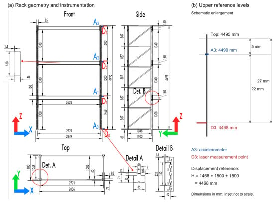
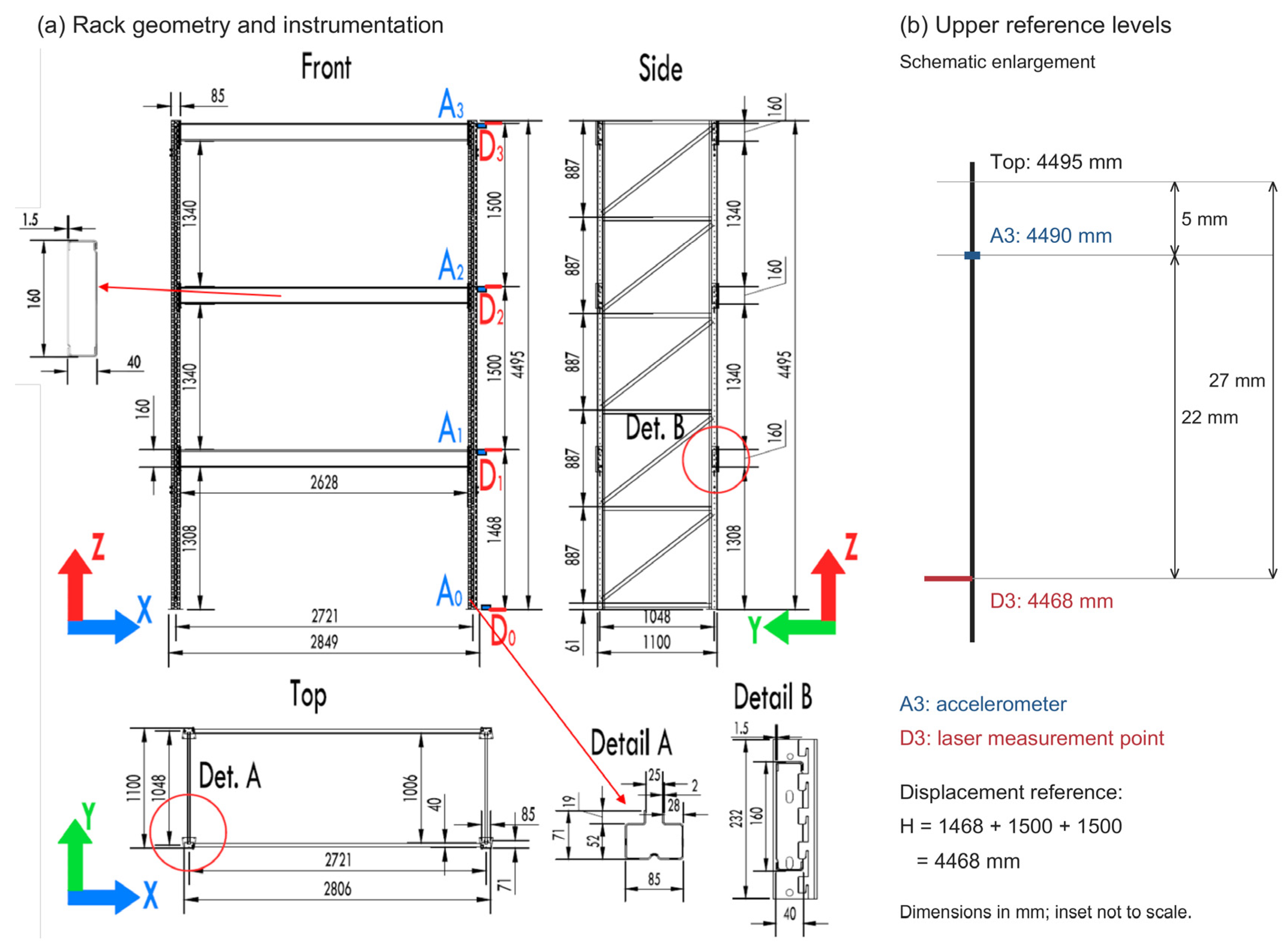
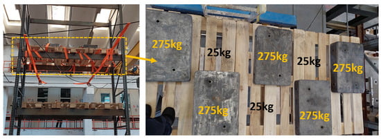
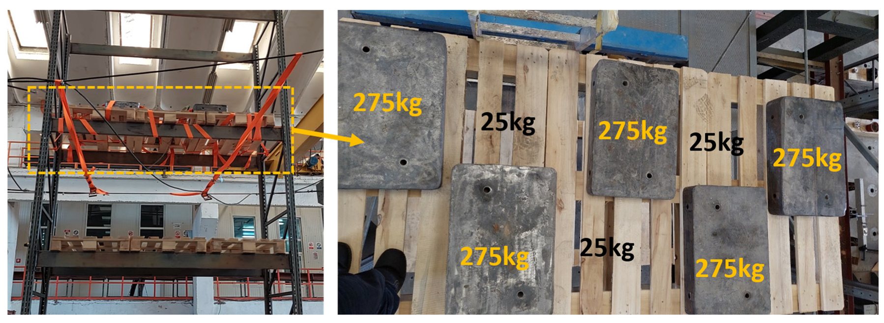
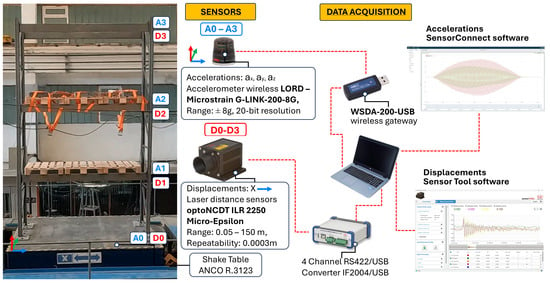
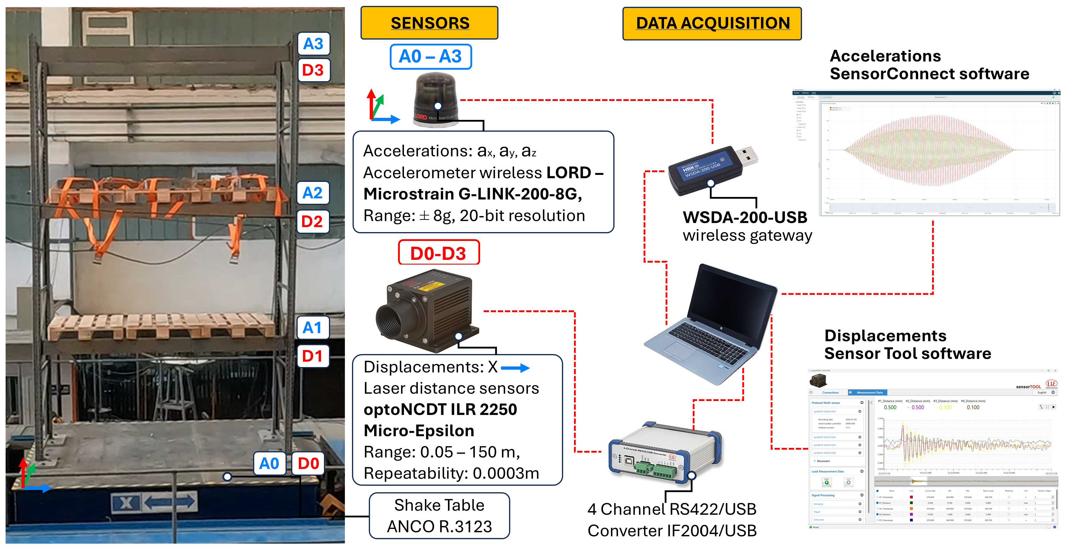
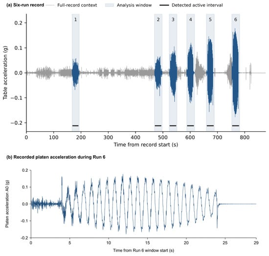
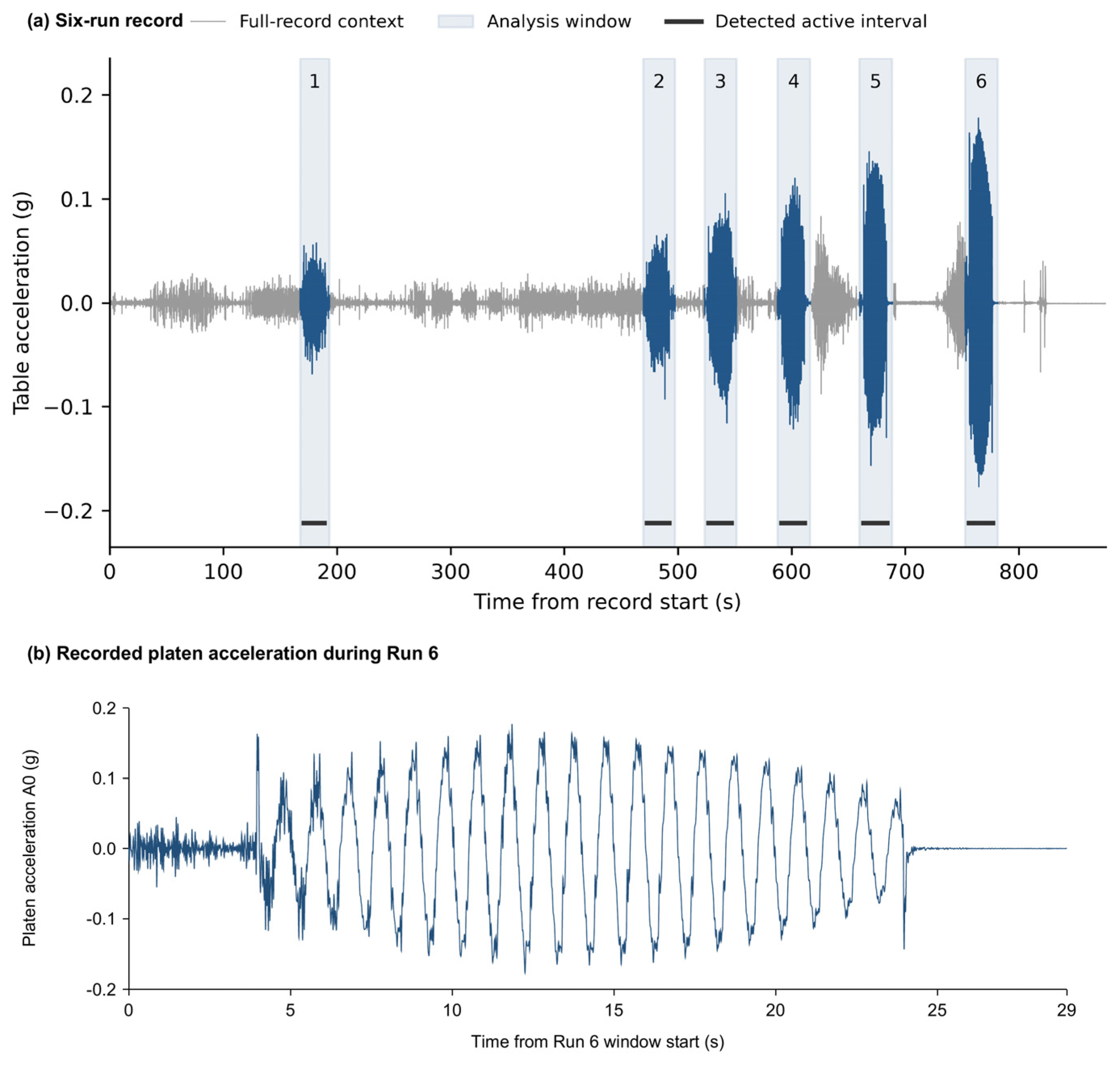
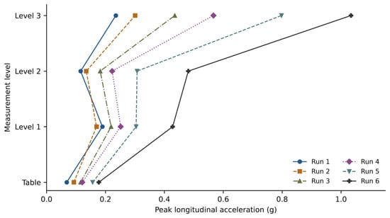
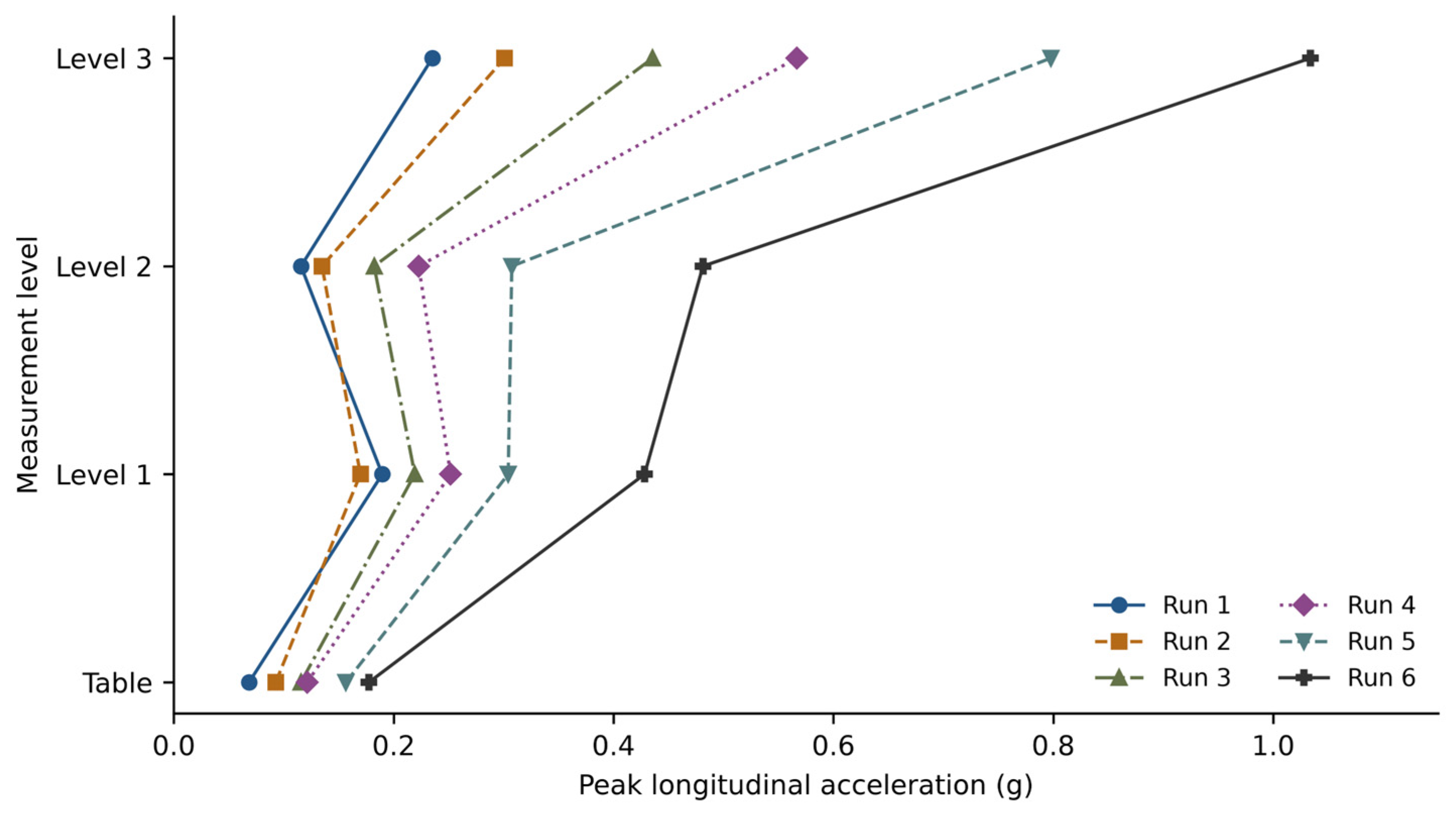
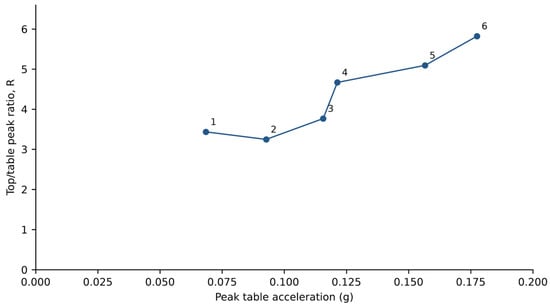
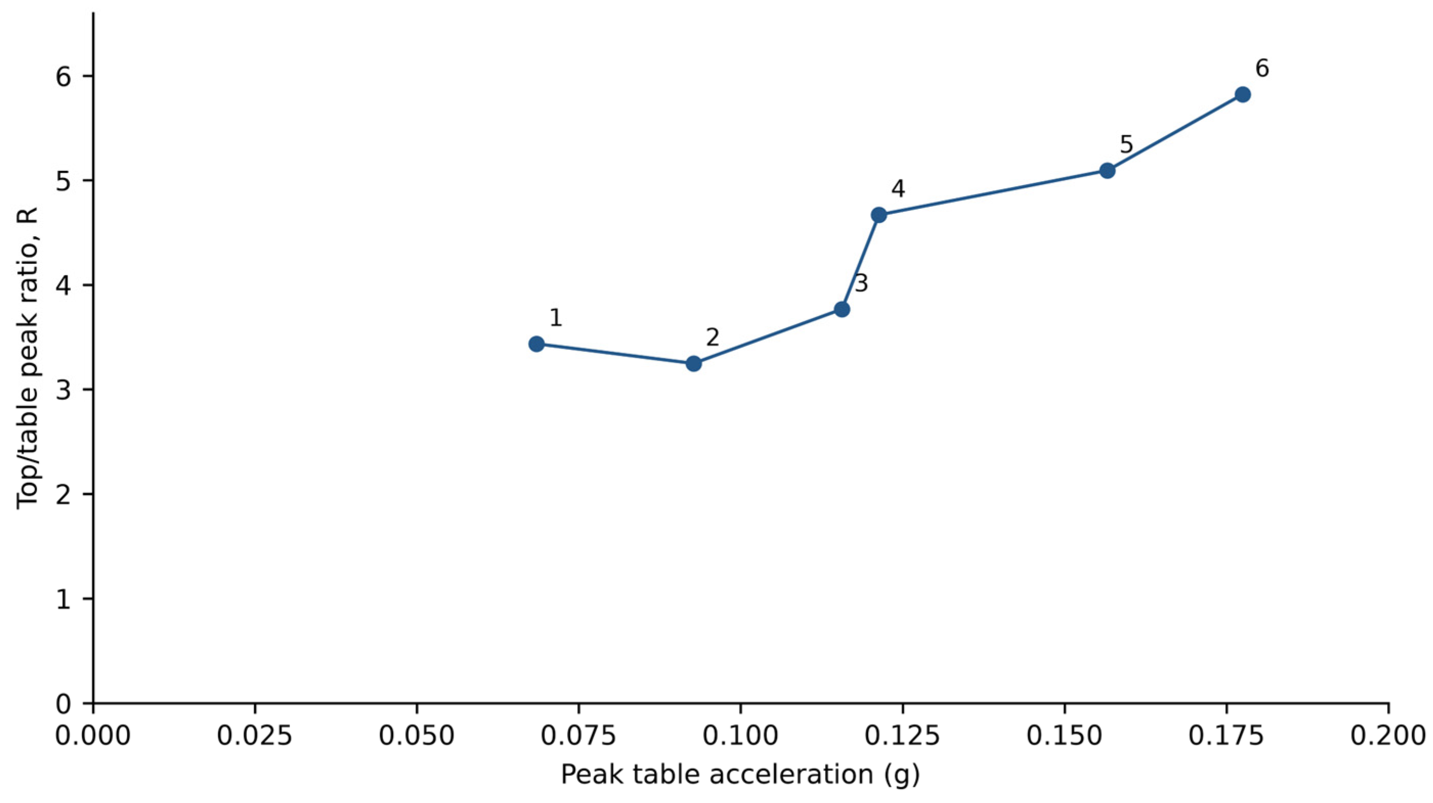
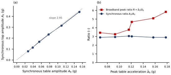
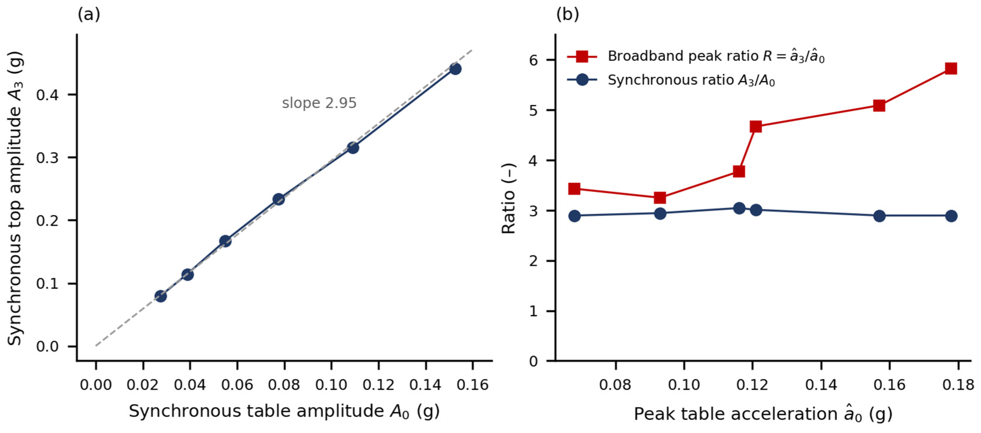
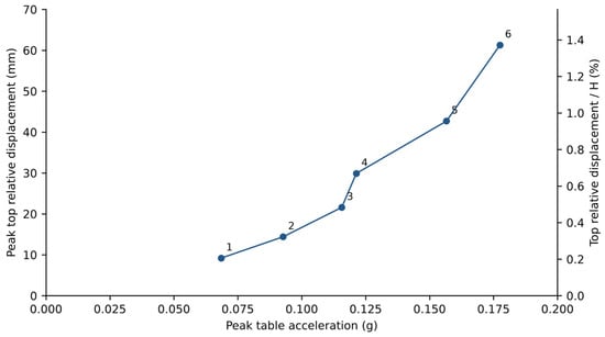
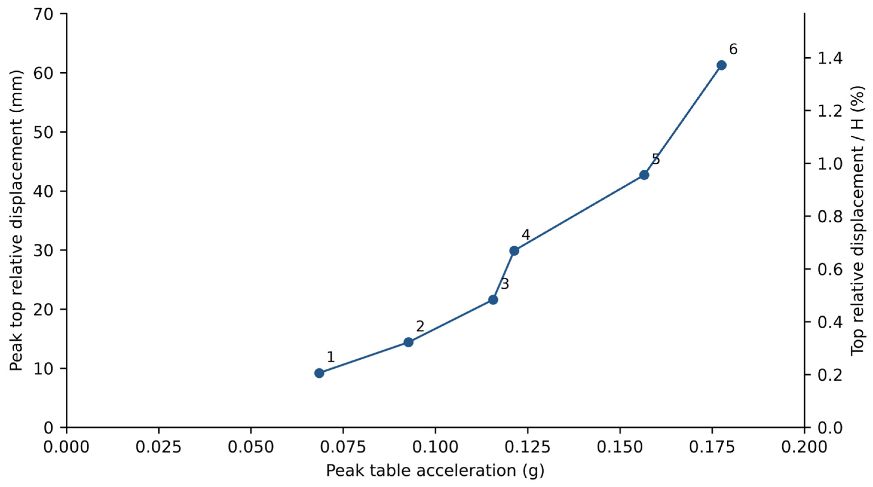
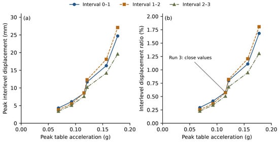
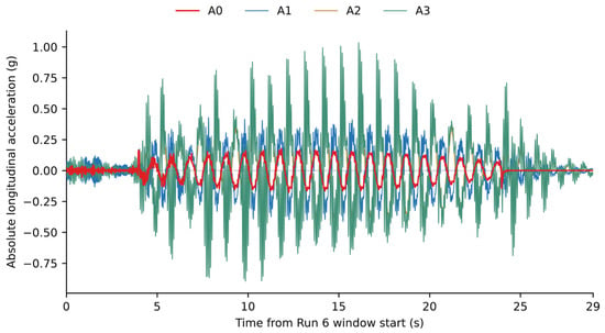
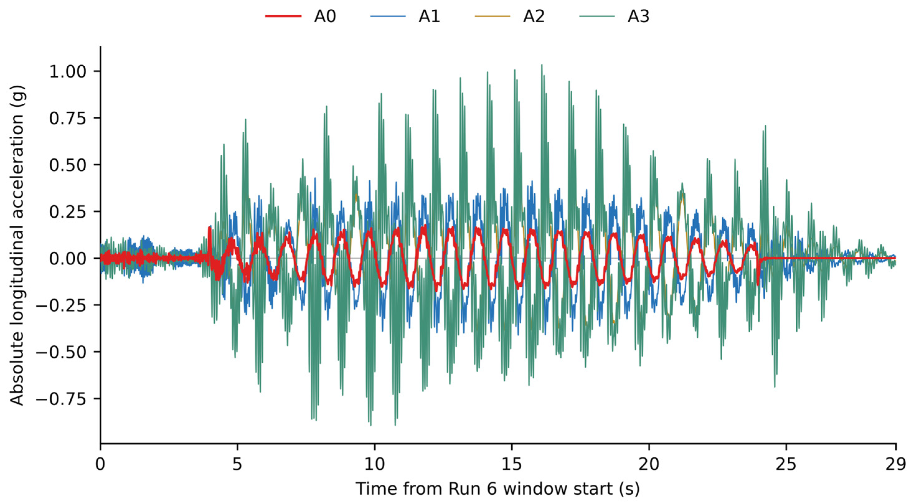
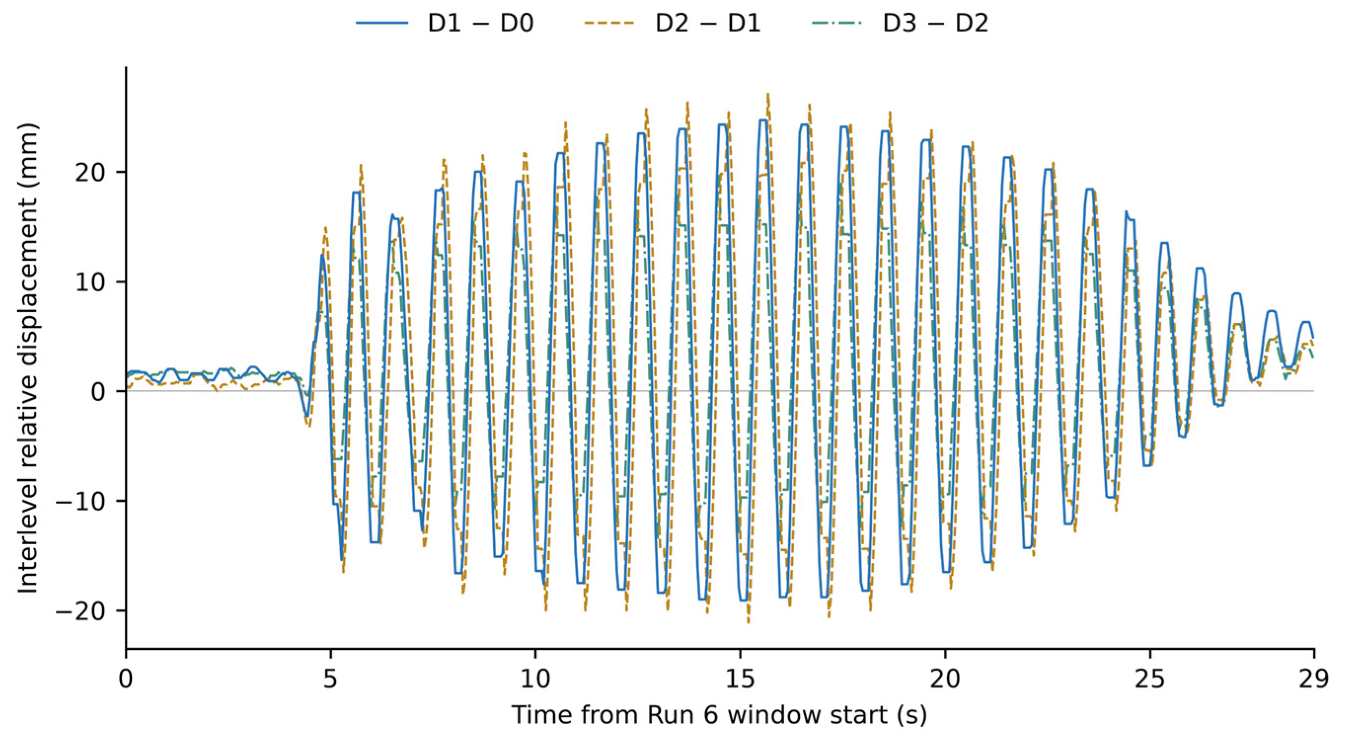
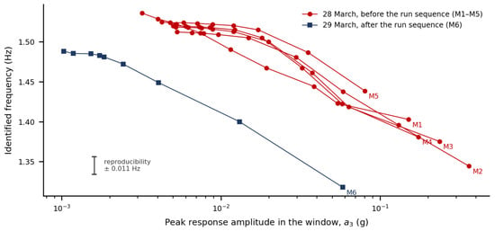
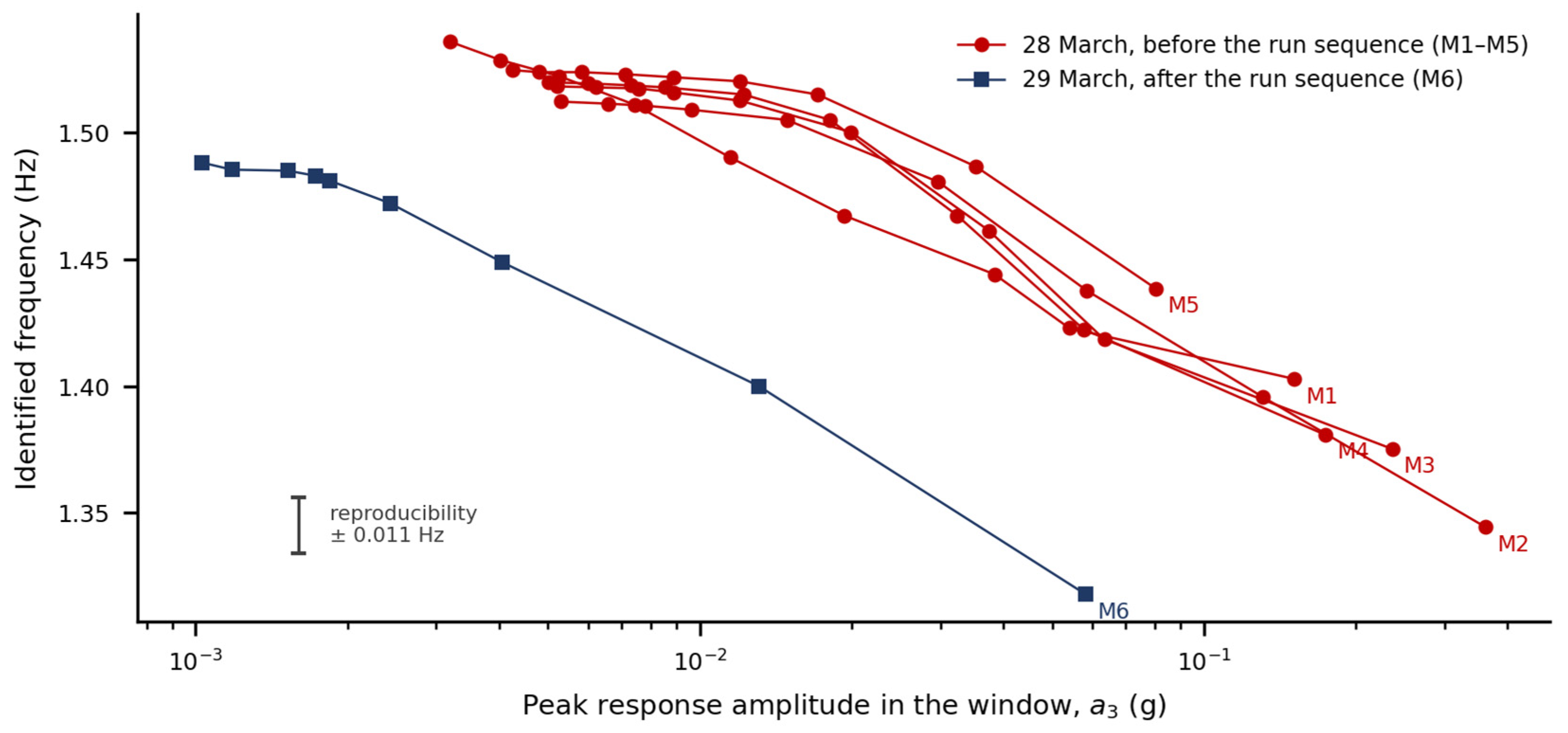
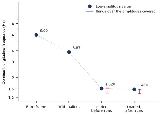

Disclaimer/Publisher’s Note: The statements, opinions and data contained in all publications are solely those of the individual author(s) and contributor(s) and not of MDPI and/or the editor(s). MDPI and/or the editor(s) disclaim responsibility for any injury to people or property resulting from any ideas, methods, instructions or products referred to in the content. |
© 2026 by the authors. Licensee MDPI, Basel, Switzerland. This article is an open access article distributed under the terms and conditions of the Creative Commons Attribution (CC BY) license.