


Abstract
This study evaluates Probabilistic Load-Adaptive Tree-Inspired Section Selection (LATSS) for constrained sizing of six large trusses. Finite-element utilization ratios guide probabilistic growth and pruning, supplemented by staged pruning, group mutation, and elitist restarts. Each comparison uses 30 independently initialized runs of 100,000 design evaluations with exactly matched initial populations. The revision adds 1200 runs, comprising corrected compression equation searches, operator ablations, a simple resizing heuristic, restart-equipped JAYA and TLBO baselines, and a 50 mm displacement sensitivity study. Corrected LATSS best volumes are 21.002 and 23.102 m3 for the 582 and 942 bar models, compared with 21.487 and 23.752 m3 under the earlier equation. LATSS achieves lower best and mean objectives than the implemented differential evolution (DE) on four models; DE performs better on the 200 and 2386 bar models. At 50 mm, the 2386 bar best volumes are 430.422 m3 for LATSS and 406.508 m3 for DE. Removing mutation substantially worsens several large model results, whereas restart and staged pruning do not improve every model. All 1200 evaluation ledgers and final vectors were audited; ten selected new designs passed independent SAP2000 response and model-constraint checks. The evidence supports problem-dependent effectiveness under explicit axial model definitions, rather than universal superiority or complete structural code compliance. Archive-selected designs remain outside controlled statistics. A separate two-model initialization study charges the generation of each warm start design to its total evaluation budget.
1. Introduction
The primary objective of truss sizing is to minimize material mass or volume while satisfying prescribed structural constraints. Changing a member’s cross-sectional area affects not only its capacity but also the system stiffness, load distribution, and nodal displacements. Consequently, the optimal design of large-scale systems cannot be reduced to assigning the smallest sections to individual members independently. As the number of members and design groups increases, these interactions create larger and more complex search spaces [1].
Sizing with continuous area variables and selecting discrete sections from commercial section catalogs constitute different optimization problems. Converting a continuous solution to standard sections can change the objective value and violate previously satisfied stress, buckling, or displacement constraints. Discrete design must retain not only cross-sectional area but also second moments of area, the minimum radius of gyration, and section identity. Mathematical programming studies of discrete sizing demonstrate the importance of treating catalog selection as an explicit design variable [2].
Derivative-free search methods are widely used for these problems. Differential evolution (DE) and harmony search (HS) are established approaches with different candidate generation mechanisms [3,4]. JAYA moves candidates toward the best solution and away from the worst, whereas teaching–learning-based optimization (TLBO) uses teacher and learner phases [5,6]. Applications to trusses include continuous and discrete sizing, as well as layout and topology variables [7,8]. The corrected multi-level and multi-point simulated annealing (CMLPSA) approach developed by Lamberti searches a population of candidate designs for truss optimization [9].
Hybrid methods and probabilistic search approaches developed for large-scale towers highlight the need to report solution quality together with the number of structural analyses [10,11]. Studies of cascade optimization and the vibrating particles system likewise show that model definition, design grouping, and the section set are decisive when interpreting results [12,13]. Discrete multi-load problems and methods based on local neighborhood rules further demonstrate that truss optimization is not confined to a single algorithm family [14,15]. Ugur, Aydemir, and Kutlu Onay enhanced the bonobo optimizer using inertia-weight strategies for the optimal design of high-dimensional trusses [16]. Their work provides a recent example of adapting search operators to high-dimensional structural design problems.
Learning-based methods have also been applied to performance-based optimal seismic design of steel frames. Degertekin and Tutar investigated JAYA for planar steel frames [17]. Degertekin, Tutar, and Lamberti studied TLBO for performance-based optimal seismic design [18] and subsequently used school-based optimization for minimum-weight design under interstory drift and strength constraints [19]. Degertekin and Tutar later developed a hybrid learning-based JAYA approach for planar and spatial steel frames [20]. Tutar evaluated JA, TLBO, and multi-class MC-TLBO on two planar steel frames in terms of structural weight and the number of analyses [21]. These studies provide methodological background; their seismic frame models and performance constraints differ from the linear-elastic truss-sizing problems considered here.
A central difficulty in comparing literature results is that models identified by the same number of members do not necessarily represent the same problem. Unless geometry, member groups, supports, load vectors, material properties, section catalogs, and constraint equations are all matched, differences in objective values cannot be attributed solely to the algorithm. Similarly, agreement between two solvers for a specified section vector does not, by itself, establish complete reproduction of a literature model or demonstrate that search methods have been compared in independent runs with equal evaluation budgets.
Engineering verification must also address failure mechanisms beyond axial stress. Experiments and finite-element studies of perforated stainless steel girders examine localized loading [22] and local web buckling [23]. These results highlight the limits of an axial truss evaluator; their plate girder capacities are not used as LATSS benchmark data.
Structural AI applications also include data-driven response prediction. Talpur et al. developed machine learning models for predicting the strength of concrete confined with sustainable natural FRP composites [24]. That problem concerns a learned response model, whereas LATSS uses direct finite-element evaluations to guide section changes. The distinction motivates explicit reporting of the structural evaluator, validation scope, and evaluation cost rather than treating different AI applications as interchangeable optimization benchmarks.
The proposed LATSS method uses utilization ratios obtained from finite element analysis to guide candidate generation. Groups with high structural demand are enlarged probabilistically, whereas groups with unused capacity are pruned. The tree analogy provides a framework for explaining the operators; the methodological contribution is not based solely on biological terminology [25]. The evaluation instead relies on a common computational budget, explicit operator definitions, and independent run records [26]. Avoiding claims of universal superiority is also consistent with the need to restrict optimization generalizations to the relevant problem classes and assumptions [27].
The study evaluates whether utilization-driven section changes provide effective constrained sizing across six fixed truss models and which components contribute under a common evaluation budget. Exact stored initial populations support comparisons with DE, classical and restart-equipped JAYA/TLBO, four single-component ablations, and a simple utilization-resizing heuristic. New searches address the corrected compression equation and a separate 50 mm displacement case. Numerical verification, source-model equivalence, and full engineering design compliance are assessed as distinct questions.
2. Materials and Methods
Figure 1 summarizes SAP2000 v24.1.0 (Ultimate, 64-bit) model construction, cross-solver response checks, the LATSS search, and verification of selected final designs. Baseline model checks in the development archive were tracked separately from verification of the current optimization results. Solver agreement and equivalence to the source problem in geometry, loading, and constraints represent different levels of verification.
Figure 1.
Model construction, response checking, optimization and final verification. SAP2000 checks cover six earlier selected LATSS designs and ten selected new designs; they do not cover every completed run or every structural failure mode.
2.1. Optimization Problem and Structural Analysis
The geometry and connectivity of each model are fixed. Each design group is represented by a continuous cross-sectional area or a section selected from a catalog. Let x denote the design vector, D the number of groups, and g(e) the group index of member e. The volume and material mass objectives are defined in Equation (1). Mass is distinct from weight as a force; values reported in kilograms or tonnes are not multiplied by gravitational acceleration.
Here, ne is the number of members, Le is the member length, and ρe is the material mass density. A linear-elastic axial truss model is solved for each candidate. Equilibrium and member stress for load case l are calculated using Equation (2).
The global stiffness matrix is reassembled and refactorized for every section vector. After all prescribed load cases have been solved, stress, displacement, and any active slenderness or buckling conditions are evaluated. Continuous variables are restricted to their physical area bounds, and discrete variables can take only valid catalog sections. For the objective function f(x) and active constraints gk(x), the general problem is expressed by Equation (3).
minx∈Xf(x), gk(x) ≤ 0, k = 1,…,ng
The analysis model represents axial behavior only. Connection details, bending, fabrication tolerances, foundation behavior, and site-specific loads are not modeled. Accordingly, feasibility in this study means compliance with the stated benchmark constraints.
2.2. Utilization Ratios and Constraint Handling
The stress utilization ratio is calculated from the most unfavorable member and load case within each group. The allowable stress depends on whether the member is in tension or compression and on the capacity equation used by the model. For the 582, 942, and 2386 bar models, the reference axial allowable stress formulation is based on Sections D1 and E2 of AISC–ASD (1989) [28]; the equations are given in Appendix A.1. Slenderness utilization is activated only when member length, the minimum radius of gyration, and an explicit slenderness limit are defined.
Only active components are used in Equation (5). Because the static 200 bar model has no separate slenderness, buckling, or displacement constraint, its group utilization consists solely of the stress ratio. For models without a prescribed displacement limit, ud is not calculated to introduce a new acceptance criterion. The maximum absolute displacement component may nevertheless be reported as response information.
When a displacement limit is exceeded, an energy-based auxiliary utilization ratio is introduced to guide candidate generation. Let Eg denote the total strain energy of the members in group g over all load cases, and Emax the largest group energy. The auxiliary ratio is defined in Equation (6).
When no displacement limit is specified, ud ≤ 1, or when Emax = 0, is used. This indicator guides only growth and pruning selections; it does not alter the physical constraints. Because load distribution is recalculated for each new section vector, the parent’s utilization ratios do not guarantee offspring feasibility. The design vector and utilization information are always taken from the same selected parent.
Denoting the normalized ratio for each active check by rk(x), the total squared violation is calculated using Equation (7). Feasibility requires every active ratio to remain at or below the tolerance threshold 1 + 10−8. Feasibility-first ranking is adopted [29]. For two infeasible candidates with equal violation, the lower objective value is used as an additional LATSS-specific tiebreaker.
2.3. LATSS Search Mechanism
The biological motivation for LATSS concerns growth and form changes associated with external mechanical stimuli. Thigmomorphogenesis and reaction wood formation are distinct biological processes [30,31]. Neither is modeled directly here; they provide only a limited analogy linking high utilization to growth and low utilization to pruning. The terms parent and offspring refer to candidate section vectors. Population restart is a numerical diversity operator rather than a biological process.
2.3.1. Initialization and Parent Selection
For continuous models, each individual’s group areas are sampled independently from uniform distributions. The initial area for individual i and group g is obtained using Equation (8). For discrete models, valid section indices are selected with equal probability. Uniform sampling of areas and uniform sampling of section indices do not produce the same initial distribution.
After feasibility-first ranking of the population, one parent is selected for each offspring. The selection categories are the best individual with probability 60%, the top ten individuals with probability 30%, and the entire population with probability 10%. Selection within the second and third categories is uniform. For population size P, M = min(10,P), and rank index j, the total selection probability is given by Equation (9).
Because the best individual can be selected through more than one category, a category probability differs from an individual’s total selection probability. Each offspring starts as a copy of the selected parent’s section vector. No crossover combines sections from different parents.
2.3.2. Probabilistic Growth and Pruning
Groups with auxiliary utilization enter the growth set, whereas groups with enter the pruning set. Groups in the narrow band between these thresholds are protected from both operations. When an eligible set is nonempty, one group is selected for the corresponding operation using the normalized weights in Equations (10) and (11). The operation is skipped when its eligible set is empty.
The area updates for the selected groups are defined in Equations (12) and (13). Here, t is the fraction of the total evaluation budget consumed before the current evaluation. The operator Π denotes enforcement of physical bounds and, for discrete models, projection onto a catalog area.
A′prune = Π[Aα(t)], c(t) = 0.75(1 − t) + 0.25t
The pruning coefficient α(t) is sampled from the three-phase schedule in Table 1. Larger area reductions are used early in the search and smaller changes later. This schedule is not an adaptation driven by success feedback. The selection exponents, thresholds, and probabilities were fixed in these experiments and are not assumed to be optimal.
Table 1.
Pruning coefficients and sampling probabilities as a function of the NFE fraction.
2.3.3. Mutation and Discrete Projection
Every tenth main offspring undergoes mutation in 1–3 groups selected without replacement from groups with different lower and upper bounds. For each selected group, Gaussian, uniform, or bounded polynomial mutation is chosen independently with probabilities of 50%, 30%, and 20%, respectively. The Gaussian standard deviation is 10% of the area range, and the polynomial distribution index is η = 20. The methodological basis and bounded implementation of these mutation schemes are described in [32,33].
Mutation is applied before structural analysis; an offspring subjected to mutation still counts as one design evaluation. In discrete models, the updated physical area is projected onto the nearest catalog area. If several sections are equally close, the parent’s section identity is retained when it is among the tied sections; otherwise, the tie is broken randomly. The magnitude of a catalog index is not interpreted as a capacity ranking. This distinction is important for sections with equal areas but different second moments of area.
2.3.4. Acceptance, Restart, and Evaluation Budget
A feasible candidate is preferred to an infeasible one. Between two feasible candidates, the lower objective value is preferred; between two infeasible candidates, the smaller total squared violation is preferred. An offspring replaces its parent when it is better, and the best-design record is retained. If 500 design evaluations elapse without a meaningful feasible improvement since the last such improvement or restart, the best 20% of the population are retained as elites and the remaining 80% are resampled. The stagnation counter also operates before the first feasible design is found.
Evaluating one design under all load cases counts as one design evaluation (one NFE). Initialization, main offspring, mutated offspring, restarts, and failed FEM attempts are all included in this count. One final evaluation is reserved for a same-solver consistency check of the selected final design. Thus, each main independent run comprises 99,999 search and initialization evaluations plus one final repeat evaluation. Unchanged offspring are also evaluated and counted. Independent SAP2000 checks are excluded from the search evaluation count. Table 2 summarizes the LATSS procedure and evaluation counter.
Table 2.
LATSS procedure and evaluation counter.
2.4. Models and Experimental Protocol
The main experimental set comprises six models with 200, 582, 942, 1938, 2386, and 3586 members. Model sizes, variable types, and objective units are listed in Table 3. Each model was run 30 times from independent uniform initializations using seeds 1–30 of the PCG64 generator. The population size was 50 for the three smaller models and 100 for the others. Each independent run retained a budget of 100,000 NFE.
Table 3.
Model characteristics and search spaces used in this study.
The original LATSS experiment contains 180 completed runs and 18 million NFE. Separate original DE and JAYA/TLBO comparisons contain 180 and 120 runs, respectively. The revision adds 1200 completed runs and 120 million NFE: 120 corrected equation LATSS/DE runs, 900 ablation and utilization-resizing runs, 120 restart-equipped JAYA/TLBO runs, and 60 displacement 50 runs. These 1680 controlled completed runs total 168 million NFE. The revised six-model LATSS summary uses the corrected 582/942 runs and the original runs for the other four models; it is not an additional experiment. Interrupted attempts, fixed vector checks, warm starts, and SAP2000 checks are excluded from these controlled budgets and retained separately. A separate, cost-accounted initialization study adds sixty model/seed pairs with three 50,000-NFE stages per pair, totaling nine million actual new evaluations. Each of the two staged policies is charged 100,000 NFE; their common generation stage is computed once and shared. It is not counted twice in the physical total, and these outcomes are not pooled with the uninterrupted run sample. Table 4 summarizes the experimental series, which are treated separately in this study.
Table 4.
Experimental series treated separately.
Model definitions were based on the geometry, grouping, material, loading, and constraint information in [7] for the 200 bar model, [11] for the 582 and 942 bar models, [10,34,35] for the large towers, and [12,13,36] for the 2386 bar model. Using source data does not establish exact equivalence between every local model and its published counterpart. The problem actually solved is defined by frozen inputs comprising coordinates, connectivity, groups, supports, loads, self-weight factors, material properties, section catalogs, and capacity equations. Local adaptations are described in Section 2.5, and the nodal loads are given in Appendix C. In particular, records from different versions of the 942 and 2386 bar section catalogs limit any claim of exact equivalence to a single published catalog. Appendix B reports the local model assignments and section vectors. Published numerical data used in the author’s selective compilations are identified explicitly in Appendix D.
The corrected 582/942 searches use the negative cubic denominator term in the AISC–ASD (1989) compression expression [28], with compression and tension slenderness limits of 200 and 300 unchanged. Both LATSS and DE were rerun from the exact original initial populations for 30 seeds per model. Earlier positive cubic records are retained only for sensitivity and provenance. The 2386 revision sensitivity retains its discrete catalog and applies a 50 mm displacement limit; it is distinct from the local 80 mm case and from a continuous area literature problem. Limited modern code formula diagnostics are not used to claim complete ANSI/AISC 360 compliance.
2.5. Model Definitions
2.5.1. Static 200 Bar Planar Truss
The first model is a static truss with 77 nodes and 29 continuous area groups [7]. Its elastic modulus is 30 Msi = 206.842719 GPa, and its density is 0.283 lbm/in3 = 7833.413033 kg/m3. Member E58 connects nodes N22 and N23, and the physical supports are N76 and N77. Out-of-plane Z restraints enforce planar analysis. The geometry is shown in Figure 2; grouping and literature-assisted design areas are provided in Appendix B.
Figure 2.
Geometry, node and member numbering, and 29 design groups of the planar 200-member truss. Drawn by the author from the computational model data; benchmark definition from [7].
LC1 applies 1 kip in the +X direction to 11 nodes, and LC2 applies 10 kip in the −Y direction to 55 nodes. LC3 is the sum of LC1 and LC2 with unit factors. The stress limit is ±10,000 psi, and the lower area bound is 0.1 in2. The 20 in2 upper bound used in the local search is not presented as a literature-defined limit. This model has no displacement, natural frequency, separate slenderness, or buckling constraint and is not the frequency-constrained 200 bar problem in [37].
2.5.2. Discrete 582 and 942 Bar Towers
The 582 bar model contains 153 nodes, 32 design groups, and a catalog of 140 AISC W-shape sections. The frozen FEM inputs use E = 210 GPa and an allowable nodal displacement of 80 mm in each coordinate direction [11]. Structural volume is minimized. The capacity calculations use Fy = 36 ksi (248.211 MPa). Elastic response agreement with SAP2000 is reported separately from these capacity checks; it does not by itself establish agreement in material yield settings or steel design checks. Figure 3 reproduces the published reference geometry [38]; the numerical model retains the frozen inputs described here.
Figure 3.
Published schematic of the 582 bar tower: (a) 3D view; (b) side view; (c) top view. Reproduced from the corresponding figure in Moez et al. [38], under CC BY 3.0 (https://creativecommons.org/licenses/by/3.0/). Cropped from the source page and resized; technical labels unchanged. Local analysis inputs are defined in Section 2.5.2.
The 942 bar model uses 244 nodes, 59 design groups, and a catalog of 295 sections. The frozen inputs specify an elastic modulus of 210 GPa, a density of 7850 kg/m3, a yield strength of 36 ksi, and a displacement limit of 381 mm. The allowable tensile stress on the gross section is 0.60Fy [28]. The BASE copy used in this study retains the assignments group 5 = members 224–235 and group 8 = members 220–223. Figure 4 reproduces a published reference schematic [39]; its displayed dimensions are not substituted for the frozen local coordinates used in the analyses. Appendix B lists the actual local member identifiers and group assignments, using the same member-to-group mapping as the analysis inputs.
Figure 4.
Published schematic of the 942 bar tower: (a) isometric view; (b) front view; (c) top view. Reproduced from the corresponding figure in Bodalal and Shuaeib [39], under CC BY 4.0 (https://creativecommons.org/licenses/by/4.0/). Cropped from the source page and resized. The displayed dimensions belong to the source schematic; the frozen local model is defined in Section 2.5.2.
The corrected 582/942 searches enforce tension slenderness ≤300 and compression slenderness ≤200, using K = 1 and the frozen catalog minimum radius. The allowable compression stress uses the negative cubic denominator in Equation (A3), switching to Equation (A4) above the critical slenderness. Displacement limits remain 80 mm and 381 mm. The elastic geometry, loads, catalog, yield strength and initial populations are unchanged. Local plate buckling and other unmodeled failure modes remain outside these axial acceptance criteria.
2.5.3. Adapted 1938 and 3586 Bar Tower Problems
The two large towers have 204 and 280 continuous area groups, respectively. Figure 5 reproduces the published 3586 bar reference schematic [10]; the local 1938 bar adaptation is defined below. The tower problem definitions are attributed to [10]. The horizontal nodal force magnitudes follow those reported by Lamberti and Pappalettere [34] in Section 9.6.2 of their book chapter. The 3586 bar model contains 897 nodes and 16 supports. The 1938 bar model retains the first 481 nodes of that geometry, translates their Z coordinates by −130 m, and restrains all translations at nodes 470–481. Removing the 12 perimeter bars at the cut plane gives a 285 m high upper-tower model with 1938 members. This truncation and support definition are local adaptations; matching the horizontal force magnitudes does not establish complete equivalence to every published tower model.
Figure 5.
Published schematic of the 3586 bar tower: (a) assembly; (b) segments; (c–f) segment and junction details; (g) key-node layout. Adapted from the corresponding figure in Degertekin et al. [10], under CC BY 4.0 (https://creativecommons.org/licenses/by/4.0/). Cropped from the source page and resized; Labels have been re-rendered for improved legibility; their numerical values are unchanged. The local 1938 bar upper-tower adaptation is defined in Section 2.5.3.
For the 3586 bar model, the total vertical load in LC1 is −47,695.5 kN. In LC2, 112 nodes on the left face each receive +0.6672 kN in X, and 112 nodes on the right face each receive −0.4448 kN in X. In LC3, 112 nodes on each of the rear and front faces receive −0.4448 and +0.4448 kN in Y, respectively. The total X load in LC2 is +24.9088 kN, and the total Y load in LC3 is zero. A zero resultant does not imply the absence of opposing nodal forces. The complete node sets were constructed from the literature face-and-floor scheme and the current geometry. These horizontal nodal forces are one-tenth of their counterparts in the thesis [35]; no claim is made that the vertical loads were scaled by the same factor.
The 1938 bar adaptation retains the same loading scheme at free nodes, with no external forces assigned to support nodes. The LC1 total is −20,047.5 kN, and the LC2 total X load is +19.1264 kN. Both LC2 and LC3 load 172 nodes. Because fixing the base excludes the flexibility of the lower tower, this definition is not treated as an exact reproduction of a separate literature 1938 bar benchmark.
Both continuous area towers use a density of 2767.991 kg/m3, a local tensile stress limit of 40 ksi = 275.790292 MPa, and a displacement limit of 406.4 mm. The reference chapter gives 275.9 MPa [34]. Equation (A6) corresponds to mean diameter divided by wall thickness Dm/t = 100; Appendix A.2 derives the coefficient. The original elastic search uses area and length directly, without a separate compression yield cap. This idealization does not establish elastoplastic safety. Area bounds are 0.1–200 in2.
2.5.4. Discrete 2386 Bar Tower
The 2386 bar model contains 516 nodes, 220 design groups, 257 W sections, and 16 supports. Although its literature context derives from large-scale tower and VPS studies [12,13], the member-to-group mapping, catalog version, and 80 mm displacement limit are components of the local model definition. The geometry is shown in Figure 6. In the PAPER_COMBINED case, a simultaneous load vector of (+5, +5, −30) kN is applied to each of 500 nodes.
Figure 6.
Local 2386-member computational model drawn by the author from stored coordinates, connectivity, restraints, and group identifiers: (a) axonometric view; (b) plan of the lowest two bays; (c) member count in each design group. Raster export: 600 dpi. Benchmark context: [12,13]; local formulation: Section 2.5.4.
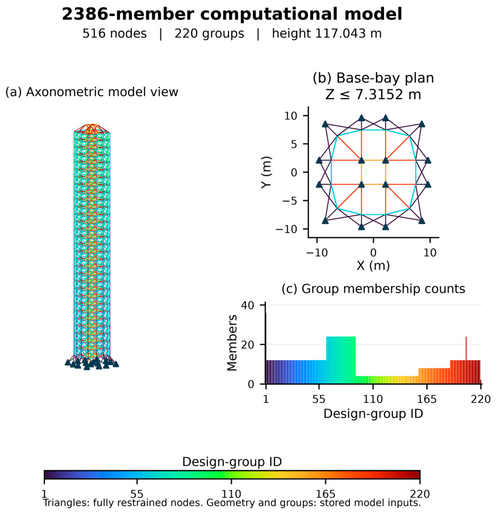
The 80 mm displacement limit is consistent with the discrete 2386 bar example of Kaveh and Ilchi Ghazaan [12], whose performance constraints refer to the first example in that article. This should be distinguished from the 50 mm limit in the continuous area problem of Shahrouzi et al. [36]. The local search uses AISC–ASD-type tension and compression capacities and an active tension-slenderness limit of 300. Compression slenderness of 200 is not an independent rejection threshold in the recorded 2386 bar search; its treatment and the subsequent Section B7 capacity check are stated in Appendix A. All 30 final designs satisfy the local 80 mm displacement limit. Catalog and group mapping differences continue to limit direct literature comparisons. A separate revision series repeats LATSS and DE at 50 mm, with 30 matched starts per method; only the displacement bound changes. No claim of equivalence to the continuous area section domain of [36] follows from this sensitivity study.
2.6. Verification, Statistics, and Computational Cost
During LATSS development, baseline axial models derived from SAP2000 models were compared in MATLAB R2021a (version 9.10.0.1602886), Python, and OpenSees 3.5.0 (64-bit). The development archive, maintained under the name LASS, records agreement in displacements and axial forces between MATLAB and Python for six baseline models, together with Python–OpenSees agreement. These records document the development of the LATSS analysis infrastructure; they are not treated as reruns of the current 180-run series in all four software environments. In particular, the earlier 200-variable definition of the 200 bar model differs from the current 29-group model, and bending response in the earlier SAP2000 frame model of the 2386 bar tower lies outside the axial solver comparison.
The current main optimization series was conducted using the Python FEM implementation. The scientific runtime documented in the project environment record was Python 3.13.15 (64-bit), with NumPy 2.5.3 and SciPy 1.18.1. Fixed designs were used to check MATLAB–Python agreement in objectives, responses, constraint decisions, and operator bounds. Because the two languages use different random-number generators, an identical seed number does not imply an identical search sequence. Final designs were checked using an independent sparse FEM solver. The selected best design for each model was also checked in SAP2000, and its section assignments, loads, supports, and response data were verified after reopening the saved files. These checks are limited to the corresponding model and section vector. The available records are not presented as a controlled speed ranking across all platforms for the six current models.
The original six selected LATSS designs have recorded SAP2000 checks. Ten selected new designs, covering corrected LATSS/DE, restart-equipped JAYA/TLBO, and the 50 mm LATSS/DE case, were newly analyzed in isolated SAP2000 copies. Input geometry, grouping, loads, supports, assigned areas, and section radii were read back, and saved results were reopened. Model acceptance was recalculated from SAP2000 responses using the explicit capacity equations. This distinguishes elastic response agreement from the selected capacity convention and broader code compliance.
NFE denotes the number of design evaluations, whereas NSA denotes the number of right-hand side solves for the load cases. For a normal evaluation, NSA = L NFE, where L is the number of load cases. The 200, 1938, and 3586 bar models have L = 3, while the 582, 942, and 2386 bar models have L = 1. Matrix factorizations and right-hand side solves were recorded separately. The counter at which the final best design was first attained is not equivalent to the cost of finding the first feasible solution or reaching a common target.
The best, mean, worst, and sample standard deviation are reported for each model. The standard deviation uses the n − 1 denominator; N/A rather than zero is used when no feasible design is available. NOE is the number of members whose stress checks exceed the tolerance. CVσ and CVU are the maximum positive exceedances of the strict stress and displacement ratio limits, respectively, expressed as percentages. CVU is undefined for the 200 bar model because it has no displacement limit.
Paired comparisons retain the identities of all 30 completed seeds. Feasibility counts are reported before objective summaries. Conditional mass comparisons use only pairs verified by both solvers and employ two-sided exact Wilcoxon signed-rank tests, with Holm adjustment across the four LATSS–JAYA/TLBO comparisons. These tests describe jointly verified subsets, not unconditional performance. An additional exact sign test ranks verified feasibility before mass and retains all 30 pairs. The four sign tests form a separate Holm-adjusted family. Runs from a single model are not treated as independent problem blocks for a cross-problem Friedman test [40,41]. The six LATSS–DE Wilcoxon comparisons form an additional, separately Holm-adjusted family; reductions and wins are signed in favor of LATSS. These per-model tests do not establish general superiority across all structural optimization problems. Revision tests use separate Holm families for the two corrected LATSS–DE comparisons, thirty LATSS–ablation/resizing comparisons, four restart baseline comparisons, and the single 50 mm comparison. Two-sided Wilcoxon tests retain paired verified objectives; all 30 feasibility-first outcomes are reported separately. Percentile 95% confidence intervals use 10,000 paired bootstrap resamples of comparator-minus-LATSS differences and are conditional on joint verification. These intervals do not include model definition uncertainty or adjustment for all possible optimizer choices.
In computational cost terms, parent ranking is O(PlogP), and group operations are O(D). For n degrees of freedom, bandwidth b, and L load cases, banded factorization costs approximately O(nb2), right-hand side solves cost O(Lnb), and extraction of member responses costs O(neL). The current catalog projection costs O(DC) for C sections. Structural solutions were not reused from a cache. Because hardware and concurrent process conditions were not controlled consistently, wall-clock times are not used to infer speed superiority. Supplementary Materials: Reproduction_Data.zip: Reproduction data supporting the analyses reported in this study.
3. Results
3.1. Solution Quality in the Main Series
Table 5 summarizes the revised primary LATSS sample: corrected searches for the 582 and 942 bar models and the original independent uniform searches for the other four models. Every row retains 30 completed runs with 100,000 NFE each. All final vectors pass both the recorded search criteria and independent sparse verification. The original positive cubic series is reported separately in Section 3.4.2, so its distribution is not silently replaced or pooled with the corrected sample.
Table 5.
Objective statistics for this study: 30 independent runs per model.
The best primary designs for the 200, 582, 942, 1938, 2386 and 3586 bar models use seeds 2, 3, 17, 28, 12 and 16, respectively. Figure 7, Figure 8, Figure 9, Figure 10, Figure 11 and Figure 12 show best-so-far feasible objectives from all 30 runs, with the best final run emphasized. Records before a run first obtains feasibility are omitted only from objective plots; first-feasible costs and success proportions are reported separately.
Figure 7.
Convergence of 30 independent LATSS runs for the 200 bar model. The thick line denotes the best run (seed 2); thin lines denote the remaining runs.
Figure 8.
Corrected expression LATSS convergence for the 582 bar model across 30 independent runs. Thin lines show the best-so-far feasible objective histories of individual runs, while the thick line highlights the run with the best final objective (seed 3). All runs have 100,000 NFE.
Figure 9.
Corrected expression LATSS convergence for the 942 bar model across 30 independent runs. Thin lines show the best-so-far feasible objective histories of individual runs, while the thick line highlights the run with the best final objective (seed 17). All runs have 100,000 NFE.
Figure 10.
LATSS convergence for the 1938 bar upper-tower model across 30 independent runs. Thin lines show the best-so-far feasible objective histories of individual runs, while the thick line highlights the run with the best final objective (seed 28). All runs have 100,000 NFE.
Figure 11.
Convergence of 30 independent LATSS runs for the 3586 bar model. Thin lines show the best-so-far feasible objective histories of individual runs, while the thick line highlights the run with the best final objective (seed 16).
Figure 12.
Convergence of 30 independent LATSS runs for the 2386 bar model. Thin lines show the best-so-far feasible objective histories of individual runs, while the thick line highlights the run with the best final objective (seed 12).
3.2. Model-Specific Convergence Behavior
For the 200 bar model, the best mass is 12,267.383 kg, the mean is 13,666.374 kg, and the sample standard deviation is 921.583 kg. Figure 7 shows the 30 runs from independent starts. The separate series initialized around the literature JA vector is excluded from this distribution, preserving the distinction between performance from random starts and local improvement of a good initial design.
With the corrected expression, LATSS obtains a best volume of 21.002278 m3, mean 22.671133 m3 and sample SD 0.815683 m3 for 582 bars. For 942 bars, the corresponding values are 23.102412, 25.999513, and 2.426649 m3. Figure 8 and Figure 9 are regenerated from the corrected search histories, rather than final vector rechecks. Although both best values improve, the 942 bar SD and worst outcome increase; the correction does not improve every summary statistic.
For the 1938 bar upper-tower model, the best mass is 171,898.150 kg, the mean is 199,455.527 kg, and the sample standard deviation is 21,082.185 kg. For the 3586 bar model, the corresponding values are 561,361.170, 625,151.214, and 41,893.189 kg. The convergence histories are shown in Figure 10 and Figure 11. Differences from literature masses cannot be attributed to algorithms without accounting for the upper-tower adaptation and the selected loading definition.
For the 2386 bar model, the best volume is 229.303037 m3, the mean is 255.754146 m3, and the sample standard deviation is 17.041056 m3. Figure 12 shows the independent runs without VPS-based initialization. The displacement limit of 80 mm agrees with the discrete benchmark in [12]. The local catalog and grouping must nevertheless be matched before numerical comparisons are interpreted as algorithmic improvements. The continuous area, 50 mm problem in [36] defines a different comparison class.
Shahrouzi et al. [36] reported JA and Jaya with passive congregation (JAPC) results over ten independent runs for a continuous area, using a 220-group definition of a tower with the same number of members. The best feasible masses are 4,820,755.4 kg for JA and 4,089,653.7 kg for JAPC (Table A18). In that source, areas vary continuously from 40 to 1600 cm2, and displacement in each direction is limited to 50 mm. The discrete W sections and 80 mm limit used here define a different feasible region; those masses are therefore not converted into a direct performance ranking against the LATSS volume results.
3.3. Independent SAP2000 Checks and Additional Capacity Verification
Table 6 combines selected design responses for the revised primary LATSS sample. The 582/942 rows use newly analyzed corrected search designs; other rows retain their recorded earlier SAP2000 results. The first-attainment fields are retained only where directly audited and otherwise shown as N/A. Every selected row satisfies its stated axial constraints, but these checks do not imply SAP2000 verification of all primary runs.
Table 6.
Independent SAP2000 responses and first-attainment counters for the selected best designs in this study.
For the six selected LATSS designs, the largest recorded normalized difference between reopened SAP2000 and Python displacement fields was 9.33 × 10⁻¹¹, and the corresponding maximum across axial-stress fields was 1.78 × 10⁻¹¹. Each difference is normalized by the maximum absolute Python response of that design. Zero member bending moments confirm the intended axial idealization in these copies. Bound and catalog validity, active stress/capacity ratios, model-specific slenderness criteria, and displacement limits were checked separately using the returned responses. These checks do not include connections, local plate buckling, torsional or flexural–torsional buckling, imperfections, second-order effects, fatigue, or dynamic loading. Response agreement does not certify a general steel design check or resolve the material yield settings of every SAP model.
The maximum recorded SAP2000 displacements are 406.399966 and 406.399799 mm for the 1938- and 3586 bar models and 79.999927 mm for the 2386 bar model. The last value satisfies the 80 mm limit used here and in the discrete reference [12], but not the 50 mm limit of the distinct continuous area problem [36]. Twenty compression members of the selected 2386 bar design have L/r above 200, with a maximum of 209.23334. This does not trigger an independent rejection in the recorded search; the additional sparse-FEM Section B7 capacity check accepted the fixed design at 80 mm. It was not a new SAP2000 analysis.
The earlier corrected capacity rechecks established only that existing sections remained feasible. The new corrected 582/942 searches now provide 60 independent LATSS histories and 60 matched DE histories. Their best LATSS volumes are 21.002278 and 23.102412 m3. The 50 mm study supplies a further 60 histories; its LATSS best volume is 430.422108 m3, and its DE best volume is 406.507545 m3. The earlier 80 mm vectors remain infeasible at 50 mm and are not reclassified by the new searches. These series must remain separate because the constraints differ.
Appendix E gives selected SAP2000 response fields. The 582/942 panels are replaced with the new corrected search designs; the remaining earlier primary design panels retain their original section vectors. All ten new verification records, section assignments, and numerical fields are included in the reproduction package. Response plots do not replace equal budget optimizer comparisons.
3.4. Matched Comparisons with JAYA, TLBO, and Differential Evolution
Classical JAYA [5] and TLBO [6] were compared on the 1938/3586 models; DE/rand/1/bin [3] was compared across all six. Each method uses the exact stored 30 initial populations and 100,000 NFE. The original basic JAYA/TLBO operations are retained in Table 7. The revised six-model DE table replaces the earlier positive cubic 582/942 comparisons with corrected LATSS/DE searches, while keeping other original protocols. Restart-equipped comparisons are reported separately in Section 3.4.4. Population sizes remain 50 for 200/582/942 and 100 otherwise.
In the implemented JAYA baseline, the best and worst individuals were fixed at the start of each generation, and two random coefficient vectors were generated per generation. In the TLBO teacher phase, the teacher and population mean were fixed; each learner used a scalar coefficient and a teaching factor of either 1 or 2. During the learner phase, a different peer was randomly selected, and improving candidates were accepted sequentially. Out-of-bounds areas were clipped to their lower or upper bounds. No additional local search or restart was used. These results therefore do not reproduce enhanced or hybrid JAYA/TLBO variants.
Table 7.
Matched comparisons for the two large towers using 30 runs per method and 100,000 NFE per run.
The previously completed LATSS–JAYA–TLBO comparison contains 180 final designs across the two towers; all underwent independent sparse-FEM checking. LATSS and JAYA passed 30/30 checks on each model. At the recorded tolerance of 10−8, banded and sparse decisions differed for five TLBO designs of the 1938 bar model and fifteen of the 3586 bar model. The largest solver differences in maximum utilization were 2.85 × 10⁻¹⁰ and 5.61 × 10⁻¹⁰, respectively. At a diagnostic tolerance of 10−7, all 30 TLBO designs on both models pass both checks; at zero tolerance, the counts are 2/30 and 4/30. These changes identify numerical boundary sensitivity, not large physical constraint violations. The original acceptance tolerance and conditional statistics are retained.
LATSS obtained lower best verified masses than the implemented JAYA and TLBO baselines. Conditional paired Wilcoxon tests support lower mass within the jointly verified subsets, with Holm-adjusted p-values of 7.45 × 10⁻⁹ against JAYA on each model, 2.38 × 10⁻⁷ against TLBO on the 1938-bar model, and 6.10 × 10⁻⁵ against TLBO on the 3586 bar model. In the all-30 feasibility-first comparison, LATSS wins 30/30 pairs against JAYA on both models and 29/30 and 30/30 pairs against TLBO. These findings are specific to the recorded implementations, initialization, budgets, and acceptance convention. New JAYA and TLBO designs have not been checked in SAP2000.
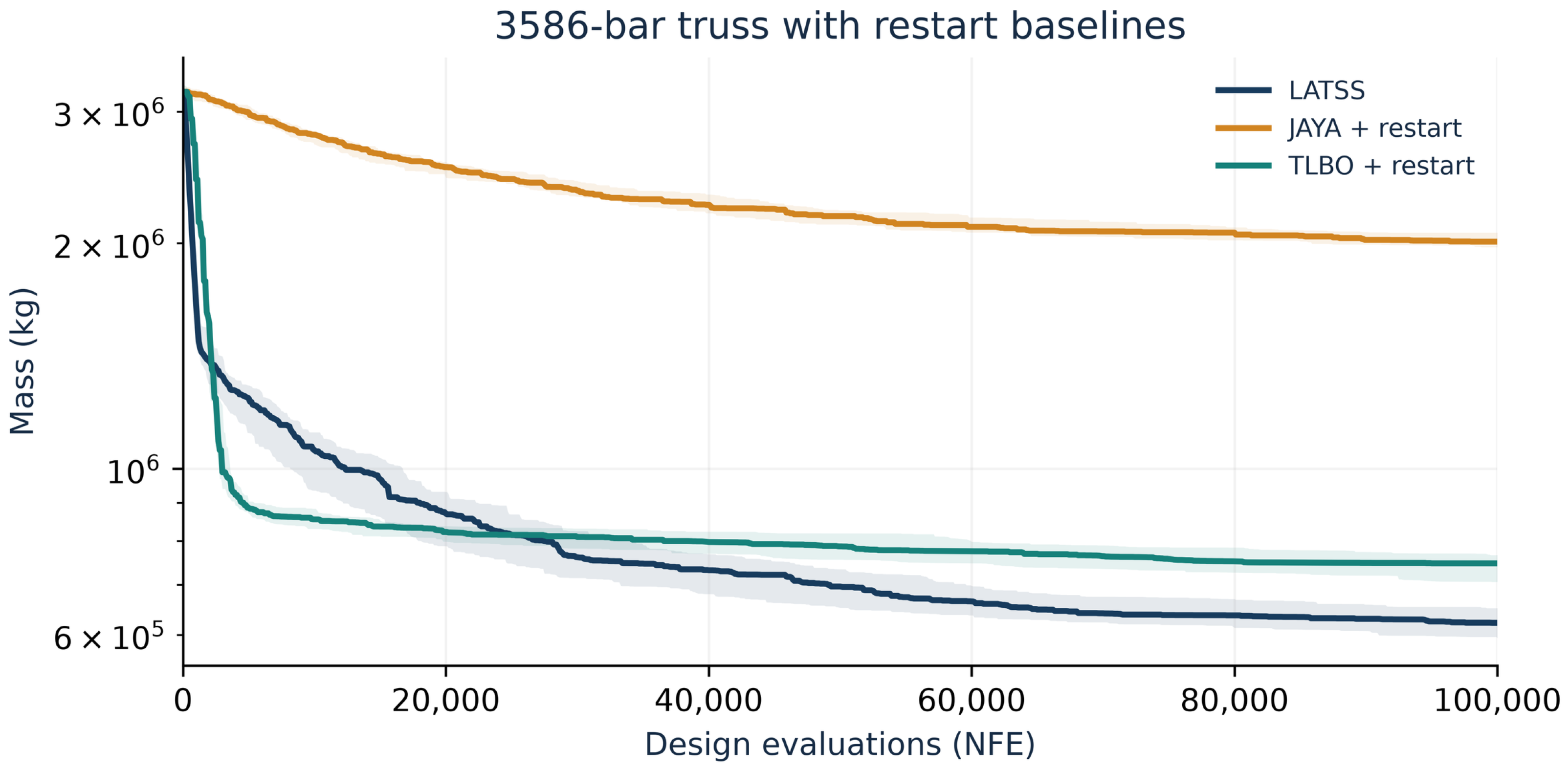
Figure 13 and Figure 14 show LATSS with restart-equipped JAYA/TLBO on the two towers. Every method retains all 30 completed runs. Lines and bands denote the median and interquartile range of search-feasible best-so-far objectives; curves begin at the first checkpoint where every plotted run has a feasible incumbent. The enhanced series is distinct from the basic implementations in Table 7.
Figure 13.
LATSS and restart-equipped JAYA/TLBO convergence for the 1938 bar model. Median and interquartile range are calculated across all 30 runs per method. Curves begin at 100 NFE; the objective axis is logarithmic.
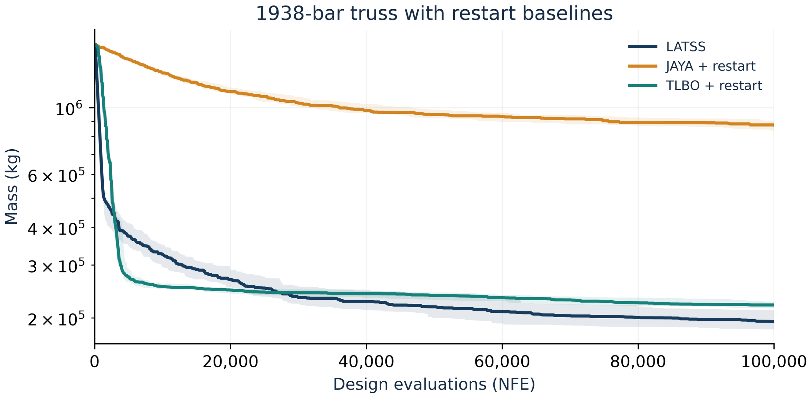
Figure 14.
LATSS and restart-equipped JAYA/TLBO convergence for the 3586 bar model. Median and interquartile range are calculated across all 30 runs per method. Curves begin at 100 NFE; the objective axis is logarithmic.
3.4.1. Differential Evolution Protocol and Six-Model Results
DE uses three distinct donors excluding the target individual, mutation scale F = 0.5, and binomial crossover probability CR = 0.9, with at least one donor coordinate forced into each trial. Donors are drawn from the frozen population at the start of each generation. Continuous variables are clipped to their bounds; discrete catalog index variables are clipped and rounded to the nearest integer. The same feasible-first selection key is used by all methods. Initialization and one final repeat evaluation are included in the 100,000 NFE; sparse verification is additional. No polishing, restart, or convergence-based early stopping is used in DE. Exact equality of all 180 initial populations and all model/engine hashes was checked. Every DE evaluation ledger contains 100,000 sequential records, and all 180 final designs passed independent sparse-FEM checking at the original tolerance. The selected corrected 582/942 and 50 mm 2386 DE designs have new SAP2000 checks. The 200 bar and 80 mm 2386 DE designs retain sparse-FEM verification only. Table 8 summarizes the six-model comparison between LATSS and DE using identical initial populations and 100,000 NFE per run.
Table 8.
Six-model LATSS–DE comparison under identical initial populations and 100,000 NFE per run.
Both methods have 30/30 verified designs per model. The 582/942 rows use new corrected equation runs; the other rows retain their original inputs, including 80 mm for 2386. Means and sample SD include all 30 designs. These locally controlled comparisons do not reproduce every literature benchmark.
Reduction is 100 × (DE − LATSS)/DE for each matched seed. The six revised primary model comparisons form one Holm-adjusted family in Table 9. Supplementary corrected-series contrasts additionally retain their separately declared two-comparison family. All thirty paired final designs are independently verified; these within-model tests do not imply cross-problem superiority.
Table 9.
Paired LATSS–DE comparisons of final verified objectives.
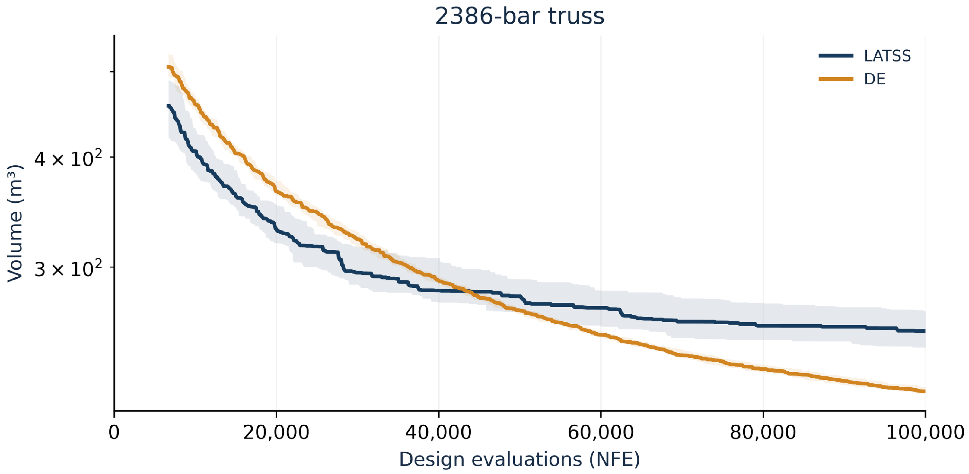
LATSS has lower best and mean objectives on the 582, 942, 1938, and 3586 bar models. DE performs better on the 200 and 2386 bar models. For the 200 bar model, the DE best and mean masses are 11,549.488043 and 11,579.805312 kg, compared with 12,267.382926 and 13,666.373994 kg for LATSS. Both algorithms’ raw 200-bar objectives were converted from lbm using 0.45359237 kg/lbm. On the 2386 bar model, DE obtains a best volume of 212.112927 m3 and a mean of 217.182316 m3, compared with 229.303037 and 255.754146 m3 for LATSS. The best DE volume is 7.50% lower than the best main-series LATSS volume. Archive-selected LATSS v2 values are outside this equal budget comparison and cannot be substituted for main-series runs. Figure 15, Figure 16, Figure 17 and Figure 18 show the matched LATSS–DE convergence histories for the 200, 582, 942, and 2386 bar models, respectively.
Figure 15.
Matched LATSS–DE convergence for the 200 bar model. Median and interquartile range across all 30 runs; logarithmic objective axis. Curves start at 300 NFE, when all runs have search-feasible incumbents. The original model protocol is retained.
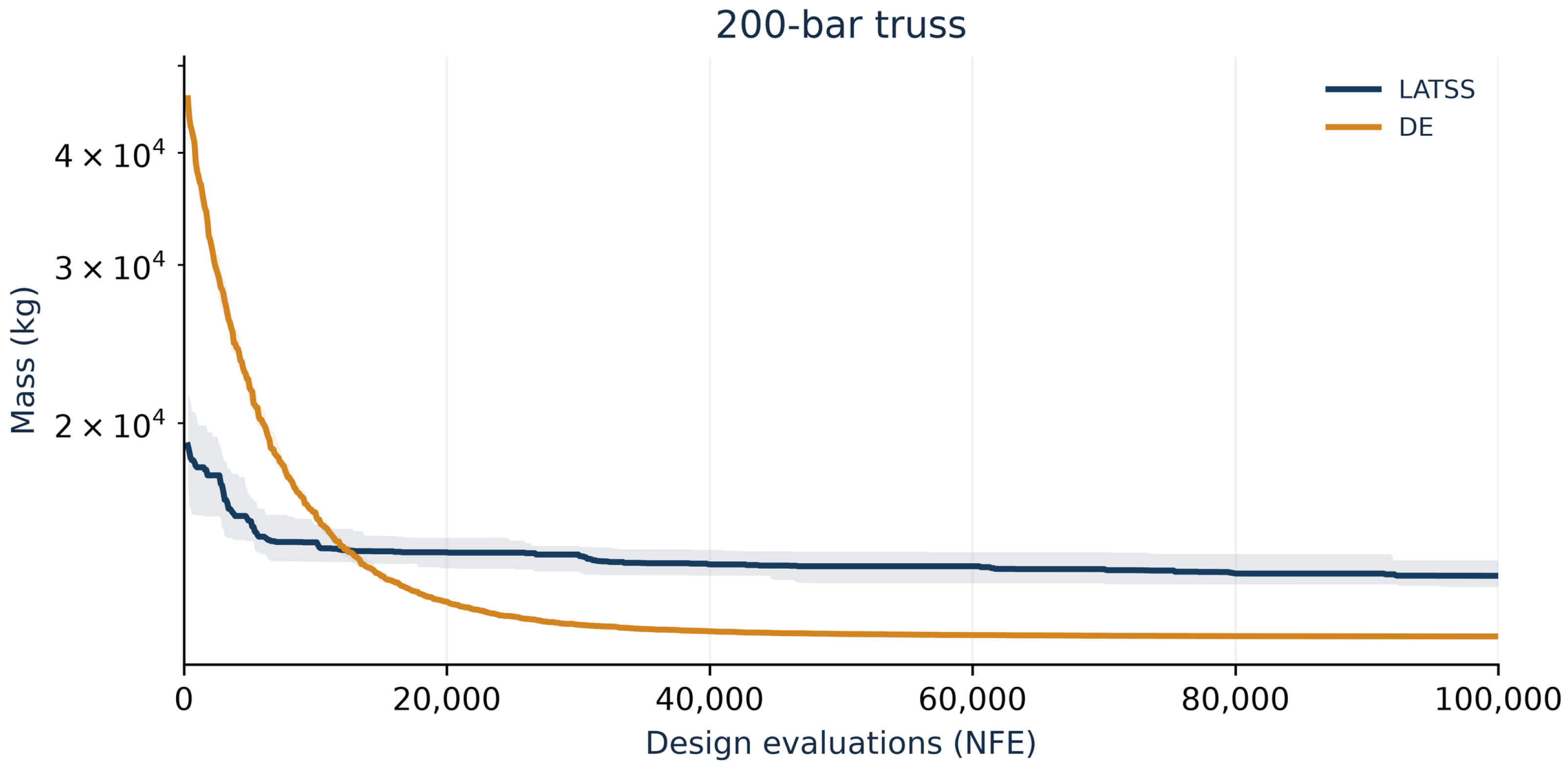
Figure 16.
Matched LATSS–DE convergence for the 582 bar model. Median and interquartile range across all 30 runs; logarithmic objective axis. Curves start at 300 NFE, when all runs have search-feasible incumbents. The corrected compression expression is used.
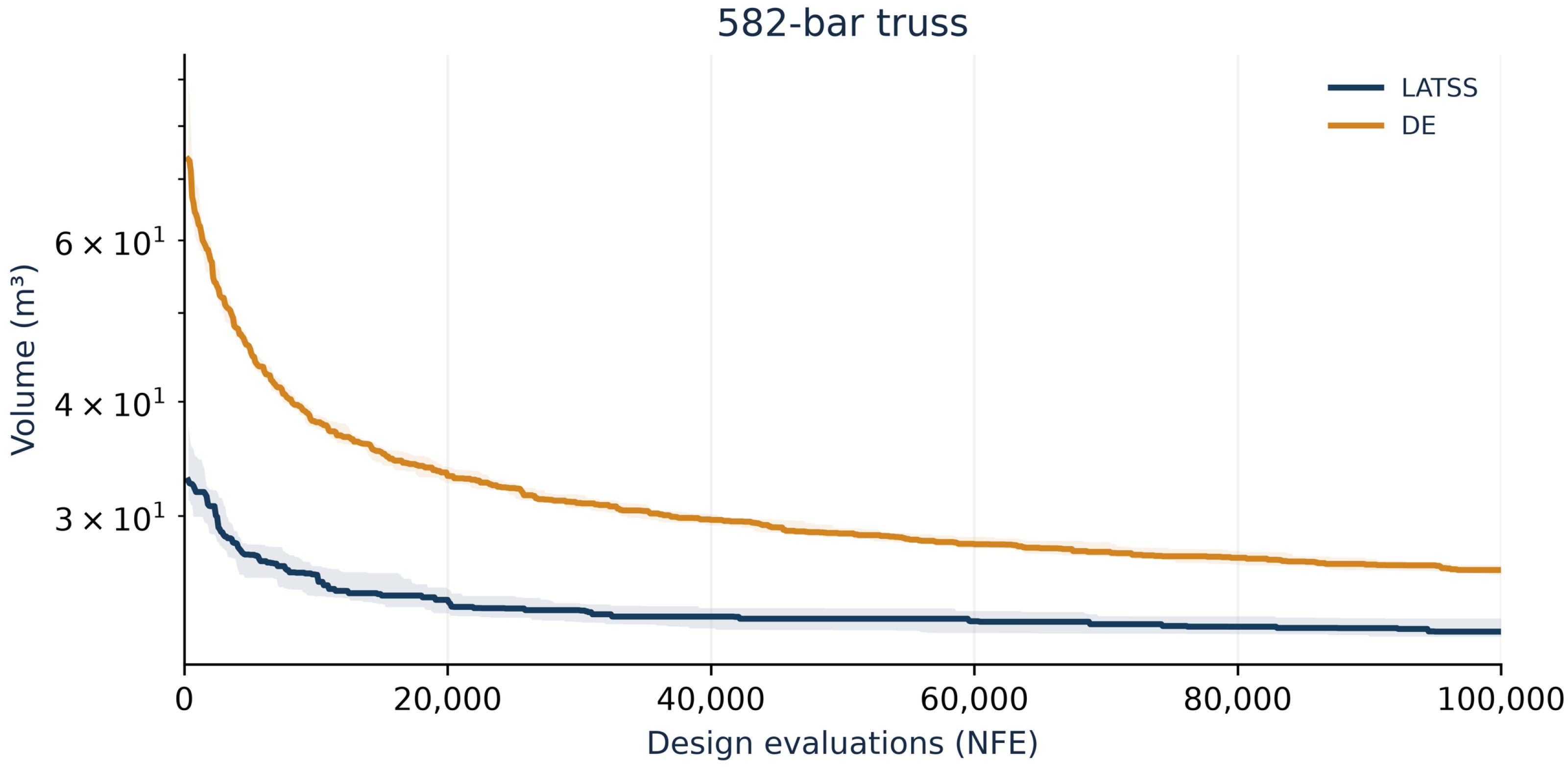
Figure 17.
Matched LATSS–DE convergence for the 942 bar model. Median and interquartile range across all 30 runs; logarithmic objective axis. Curves start at 800 NFE, when all runs have search-feasible incumbents. The corrected compression expression is used.
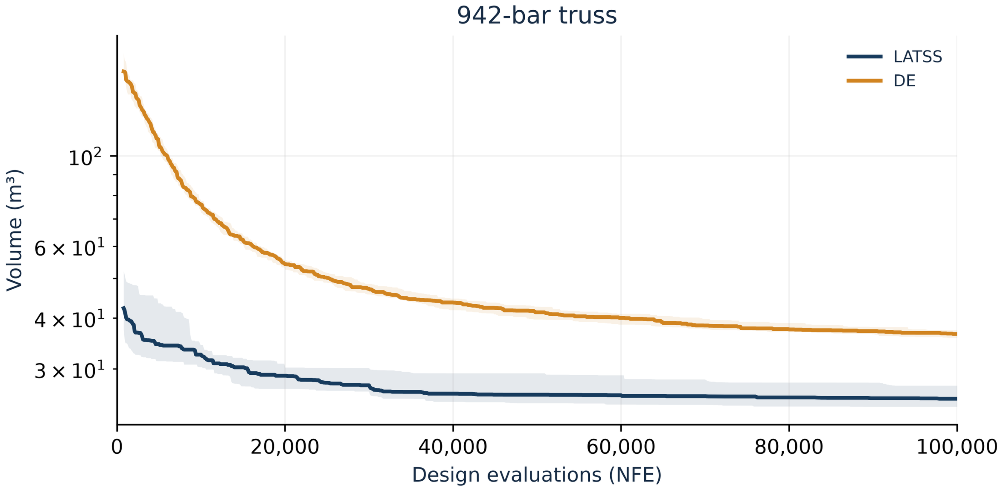
Figure 18.
Matched LATSS–DE convergence for the 2386 bar model. Median and interquartile range across all 30 runs; logarithmic objective axis. Curves start at 6700 NFE, when all runs have search-feasible incumbents. The original model protocol is retained.
3.4.2. Searches with the Corrected Compression Equation
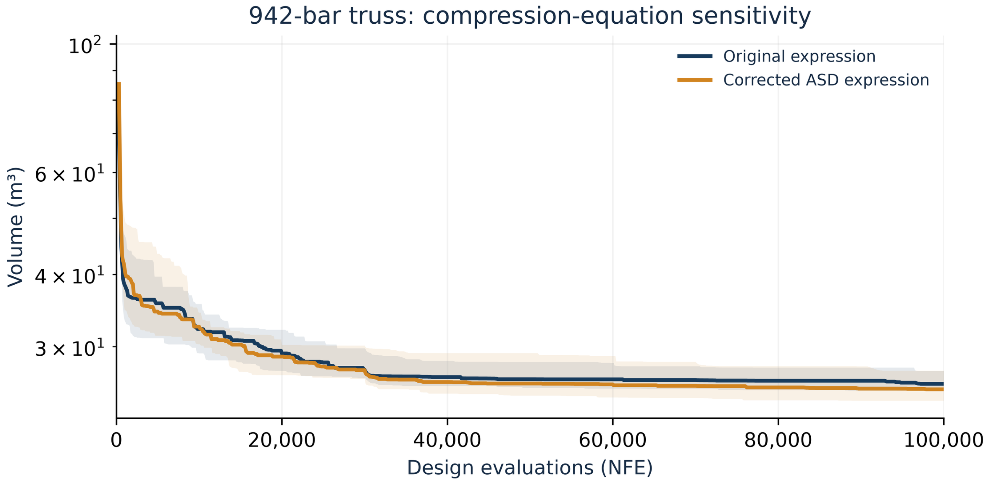
Thirty LATSS and thirty DE searches were repeated for each of the 582/942 models with the negative cubic term active throughout. The original and corrected LATSS initial populations are byte-identical. The corrected best volumes decrease by 2.257% and 2.737%, respectively; means decrease by 0.872% and 2.216%. The 942 bar worst value increases from 32.080526 to 32.462629 m3. Thus, final vector feasibility checks alone would have missed changes in search behavior and dispersion. Table 10 compares the original and corrected compression-equation LATSS results for the 582 and 942 bar models using paired initial populations. Figure 19 and Figure 20 show the convergence histories for the 582 and 942 bar models, respectively, using the corrected compression equation.
Table 10.
Original and corrected expression LATSS searches with paired initial populations.
Figure 19.
Compression equation sensitivity for 582 bars. Median and interquartile range across thirty runs per expression; the curves represent separate searches, not rechecks of final sections.
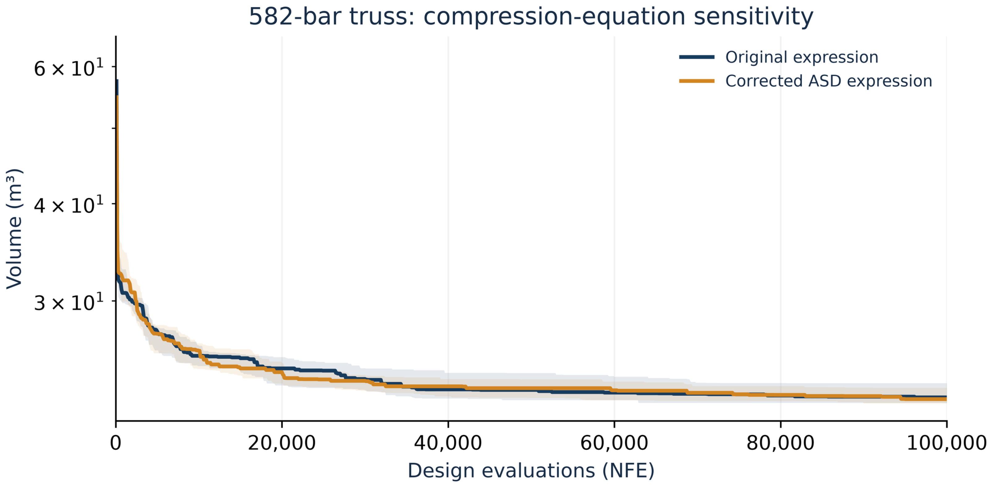
Figure 20.
Compression equation sensitivity for 942 bars. Median and interquartile range across thirty runs per expression; the curves represent separate searches, not rechecks of final sections.
3.4.3. Operator Removal and Simple Utilization Resizing
Four alternatives remove only one feature: use uniform probabilities within the existing growth/pruning eligible sets; disable restart; disable group mutation; or replace staged pruning with fixed α = 0.85. All other operators, initial populations, and evaluation budgets are retained. The fixed-pruning variant still consumes the original coefficient draw before overriding its value, preserving that random draw in the implementation. Uniform group weighting retains utilization-based eligibility and growth magnitude, so it is not a complete removal of engineering information.
A fifth alternative updates all group physical areas simultaneously using the multiplier clip(max(group utilization, displacement ratio), 0.5, 2), followed by the same bounds/catalog projection and feasibility-first selection. It cycles through the population without mutation or restart and evaluates even unchanged candidates. This explicitly defined simple heuristic is not asserted to be a universal canonical fully stressed design method.
Means and SD in Table 11 are conditional on independently verified feasibility, while every success denominator remains thirty. Simple resizing verifies 27/30 designs on the 200 bar model and 8/30 on the 942 bar model; its successful subset averages must not be read as unconditional superiority. All other reported alternatives verify 30/30 per model. Supplementary paired tests retain feasibility-first outcomes for all thirty seeds as well as conditional objective contrasts.
Table 11.
Equal budget alternatives with exactly matched initial populations. Units are kg for 200/1938/3586 and m3 otherwise.
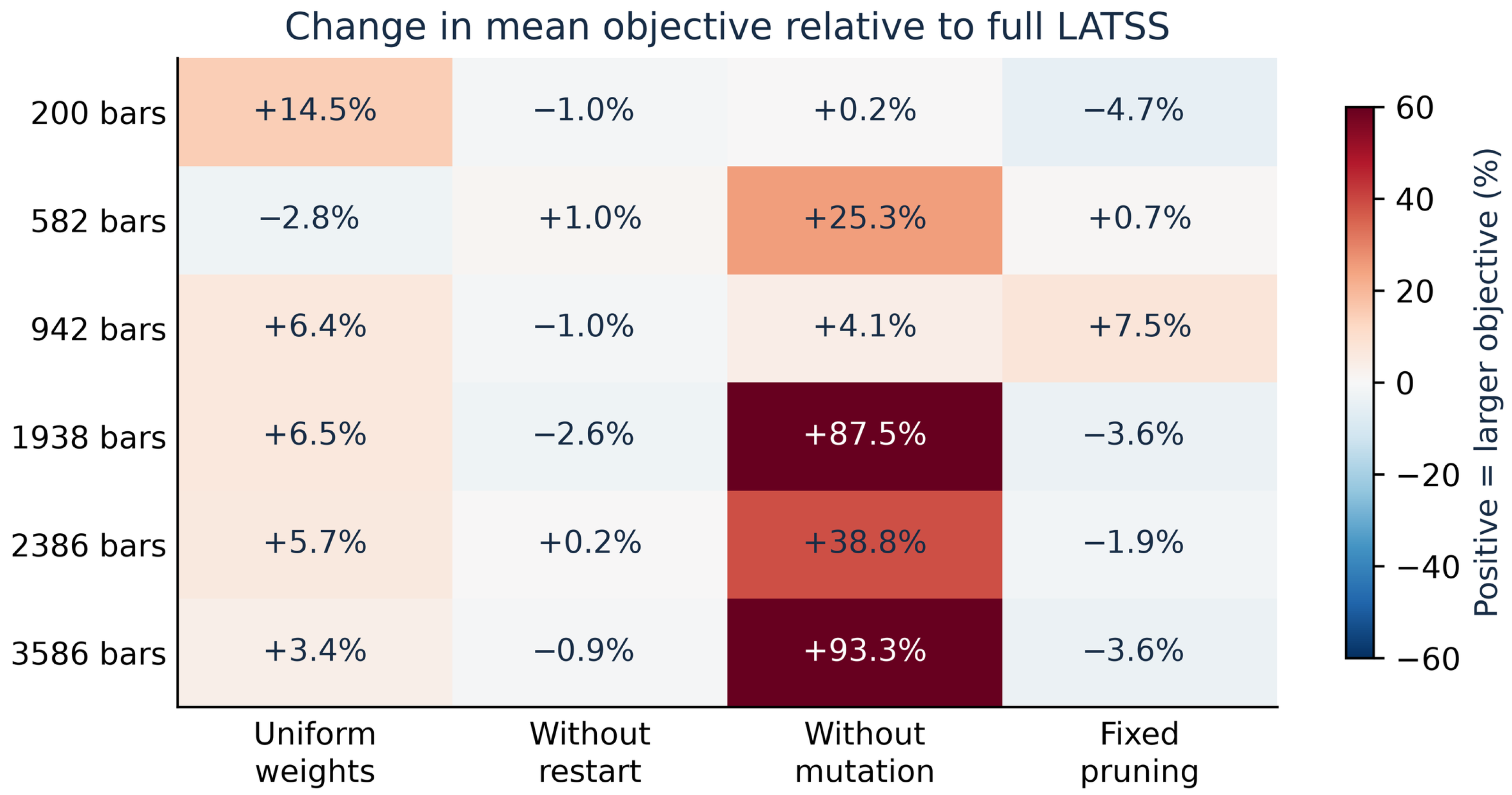
Figure 21 summarizes the percentage changes in mean objective for the four operator variants. Mutation removal increases mean objectives, particularly on the 1938, 2386, and 3586 bar models. Conversely, uniform group weights improve the 582 bar mean, and fixed pruning improves the 200 and 3586 bar means. Removing restart improves some distributions. These are component removal contrasts within a fixed configuration; they do not establish a single best component combination or isolate higher-order interactions. Six model-specific convergence figures and the full adjusted comparisons are supplied in the supplement.
Figure 21.
Percentage change in mean objective when one LATSS feature is changed. Positive values indicate a larger objective than full LATSS. All cells use thirty independently verified designs; the simple resizing heuristic is excluded because its success rates differ.
3.4.4. Restart-Equipped JAYA and TLBO
The basic JAYA/TLBO candidate operations are supplemented by the same 500-NFE feasible improvement stagnation trigger, 20% elite retention, and 50/30/20 restart mixture as LATSS. The mixture generates uniform designs, local perturbations of retained elites, or a uniform fallback when no source generator is installed. Restart evaluations count toward 100,000 NFE. These are controlled restart-equipped variants, not claims to reproduce a published enhanced algorithm; elitist TLBO variants in the literature [42] provide distinct methodological context. Table 12 compares LATSS with restart-equipped JAYA and TLBO for the 1938 and 3586 bar tower models using paired initial populations.
Table 12.
Tower comparisons with restart-equipped baselines and paired initial populations.
All thirty restart-equipped runs per method and tower pass both solvers at the original 10−8 acceptance tolerance. Their best and mean masses remain above LATSS. The 1938-bar TLBO + restart mean is 222,376.039 kg, and the 3586-bar mean is 741,413.607 kg; the LATSS means are 199,455.527 and 625,151.214 kg. This reduces one imbalance in recovery mechanisms but does not exhaust tuning, representation, or enhancement possibilities.
3.4.5. Displacement Limit Sensitivity of the 2386 Bar Model
The displacement limit is reduced from 80 to 50 mm with geometry, loads, material, grouping, and the 257-section discrete catalog frozen. Thirty independent matched-start runs per method remain at 100,000 NFE; no warm-start vector or 80 mm final vector is injected. This is a local discrete sensitivity experiment, not a reproduction of the distinct continuous area literature definition. Table 13 compares the LATSS and DE results for the 2386 bar model under displacement limits of 80 mm and 50 mm.
Table 13.
Separate 80 mm and 50 mm searches for the frozen local discrete 2386 bar model.
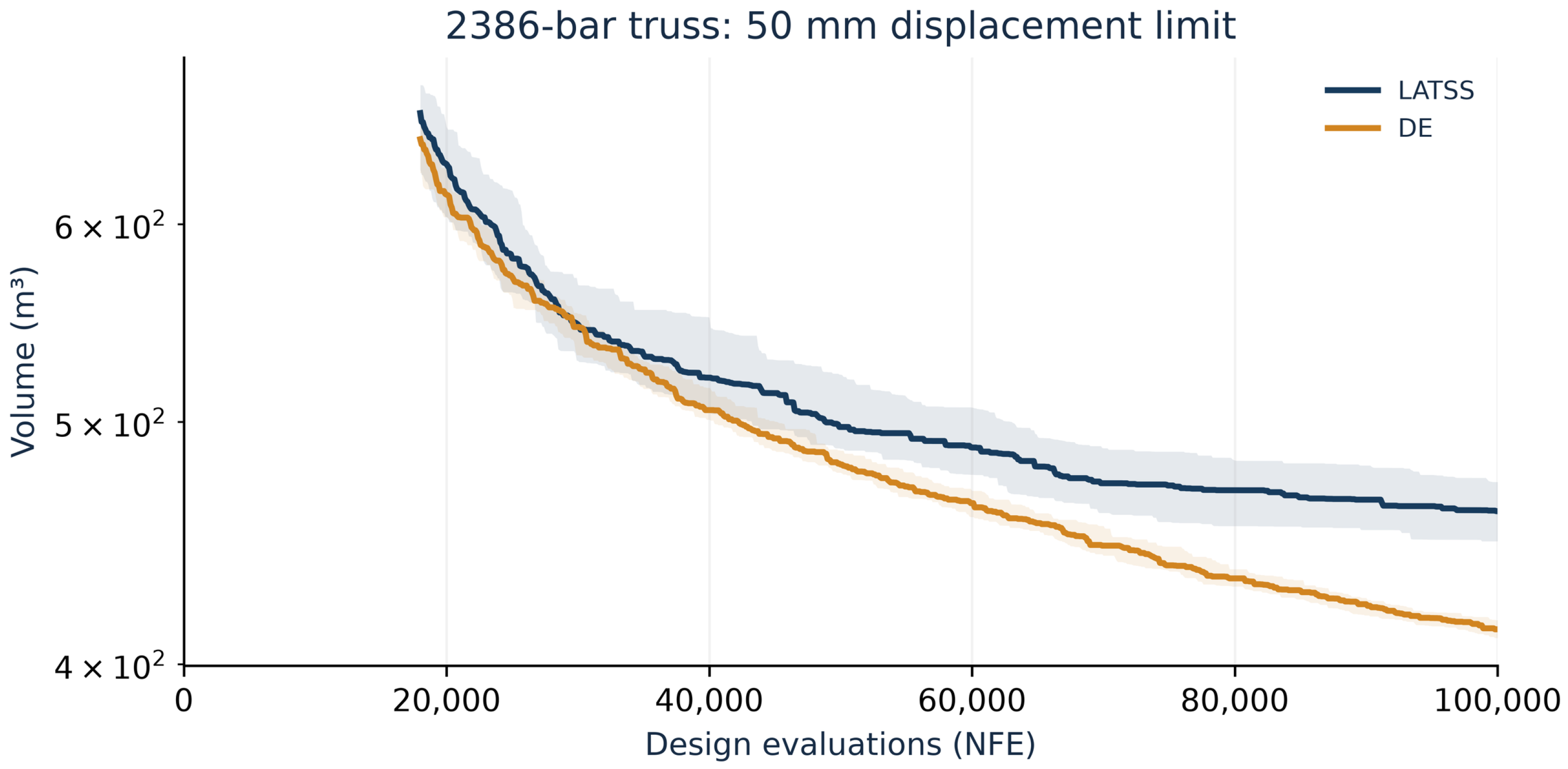
At 50 mm, DE has both a lower best volume and a lower mean volume than LATSS. The best-volume difference is 23.914563 m3 (5.56% of the LATSS best), and the paired mean comparator-minus-LATSS difference is reported with its confidence interval in the supplement. The larger volumes than at 80 mm reflect the tighter feasible region and changed search trajectory, rather than a change inobjective units. Figure 22 shows the corresponding LATSS–DE convergence histories at the 50 mm displacement limit.
Figure 22.
LATSS–DE convergence at a 50 mm displacement limit for the local discrete 2386 bar model. Median and interquartile range across thirty runs per method; the objective axis is logarithmic.
3.4.6. New SAP2000 Verification and Numerical Sensitivity
All ten selected new designs satisfy the stated axial checks recalculated from SAP2000 responses. The largest normalized displacement and stress differences are 2.890 × 10⁻¹⁰ and 5.757 × 10⁻¹¹. Each field error is normalized by the largest absolute Python component of that design. Geometry, loads, restraints, grouping, section areas, and radii were read back; original source SDB files were unchanged. These checks cover selected corrected and comparator designs rather than every final run, every ablation, or every steel failure mode. Table 14 summarizes the SAP2000 verification results for the ten newly selected designs.
Table 14.
Newly selected best designs checked in SAP2000 after reopening saved results.
The 582 bar source material record retains 50 ksi, whereas acceptance calculations use 36 ksi. The new solver comparisons do not use native steel design checks; yield strength does not enter the linear-elastic stiffness at fixed E. External capacity acceptance consistently uses the declared 36 ksi. The discrepancy is disclosed rather than treating elastic response agreement as proof that the native material yield record agrees. For continuous towers, the new SAP tube proxies use mean Dm/t = 100 to match Equation (A6).
Fresh sparse free-degree-of-freedom residuals were checked for the 480 original LATSS/DE/JAYA/TLBO final vectors and all 1200 new final vectors. Maximum load-normalized residuals are 8.36 × 10⁻¹¹ and 6.56 × 10⁻¹¹, respectively. Basic TLBO classifications change at numerical boundaries: acceptance at 10−8 is 25/30 and 15/30, while a diagnostic 10−7 threshold accepts 30/30 in both towers. Direct banded/sparse solves expose no user-set iterative convergence tolerance. Threshold sensitivity and displacement reserve checks are therefore fixed vector diagnostics, not tighter tolerance reoptimization. Complete new-run threshold and reserve counts accompany the supplement.
Fixed vector displacement reserves of 0.1%, 0.5%, and 1% change acceptance for boundary designs. For the original LATSS towers, only one 1938-bar vector retains a 0.1% reserve, and none retains 0.5% or 1%; no 3586-bar vector retains 0.1%. Consequently, unchanged engineering-margin rankings are not claimed. All thirty outcomes, conditional summaries, and paired bootstrap intervals remain available in the supplement.
3.4.7. Feasibility Discovery and Budget Dependent Outcomes
The archived ledgers distinguish first-feasible NFE from first attainment of the final best design. On the two original tower comparisons, every method has median first feasibility at one evaluation: the uniform populations already contain feasible designs. The large differences in final mass therefore primarily concern refinement rather than delayed initial feasibility. For the original stress-only 200-bar LATSS and DE series, median first-feasible NFE is 36 for both. Revised per-seed first-feasible NFE and objective values at 10k, 25k, 50k, and 100k are supplied as separate data tables. Post hoc targets are labeled as such; no target was used for early stopping or budget selection.
3.4.8. Initialization Comparison Including Design Generation Cost
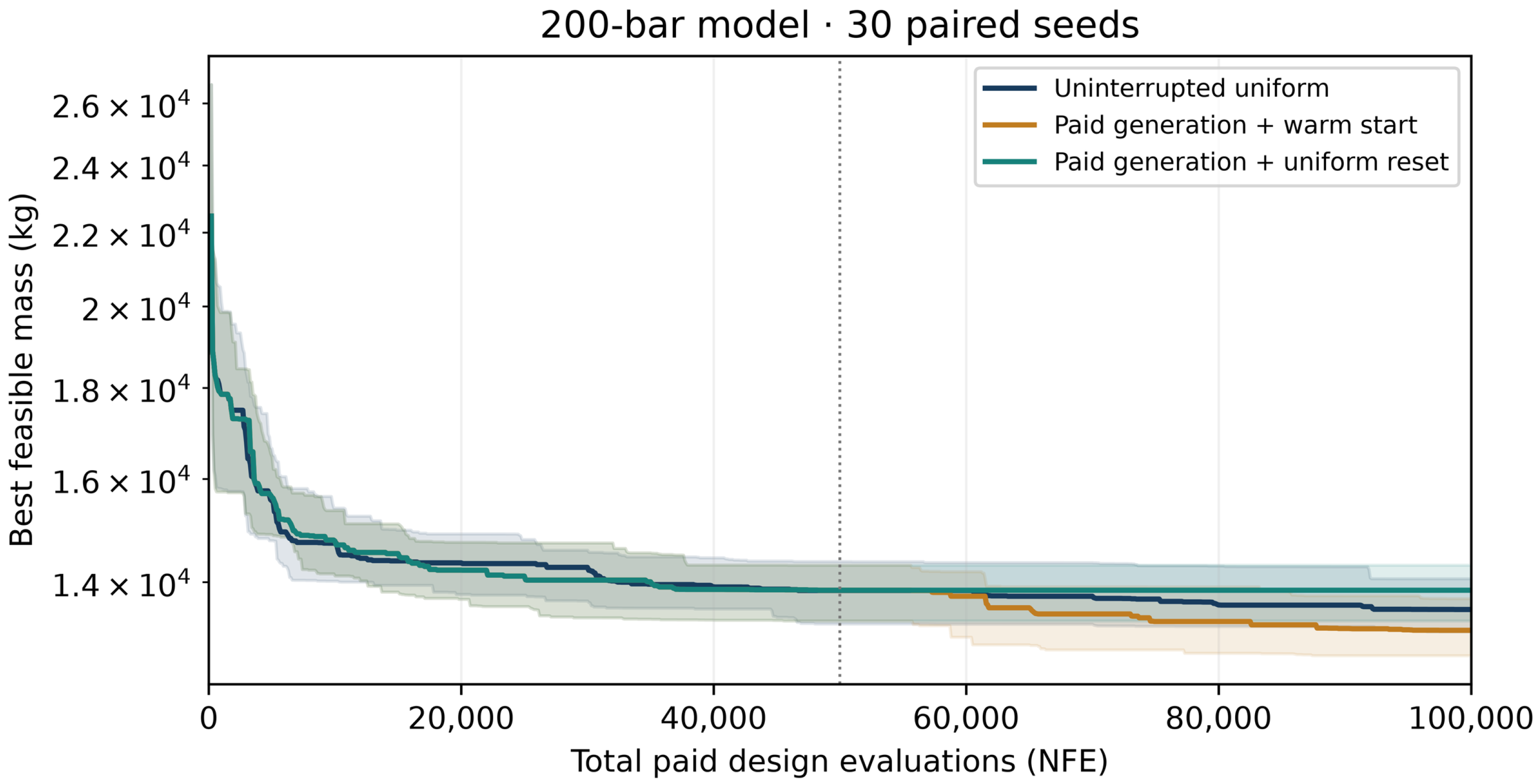
For the 200 and 2386 bar models, thirty independent paired seeds each generate a design in 50,000 NFE. Two continuations each receive 50,000 additional NFE: the warm-start continuation replaces only population slot zero with the same-seed generated design; the uniform reset control retains the exact stored uniform population. Both consume the same initialization random draws. The generation stage is shared, but its full 50,000-NFE cost is charged to each policy. Both policies therefore cost 100,000 NFE end to end, while their paired physical execution uses 150,000 rather than 200,000 evaluations. Across sixty pairs, this is nine million new physical NFE, with all 180 stage ledgers audited. Historical archive vectors are not used.
The reported incumbent is the best-verified design across both paid stages, even when it originates in generation. Each stage includes initialization and one final repeat, and uses its own 50,000-NFE three-phase schedule. Warm versus uniform reset isolates elite injection under the same schedule reset; comparison with the existing uninterrupted 100,000-NFE runs additionally tests a different budget allocation. The two staged policies share preparation and must not be treated as independent samples. Seed pairs remain independent within each model.
For the 200 bar model, mean objectives are 13,265.695 for paid warm starts, 13,924.429 for the paid uniform reset control, and 13,666.374 for uninterrupted uniform search. Feasibility counts remain explicit in Table 15; conditional objective summaries do not replace the success denominators. The direction and uncertainty of each paired contrast are reported in the supplement, including cases where warm starts do not improve performance. Figure 23 and Figure 24 compare the initialization-policy convergence histories for the 200 and 2386 bar models, respectively.
Table 15.
Initialization strategies at 100,000 total charged NFE per policy. Mass is in kg for 200 bars and volume in m3 for 2386 bars; the generation-stage cost is included.
Figure 23.
Initialization policies for the 200 bar model. The horizontal axis includes all paid generation evaluations. The dotted line marks the 50,000-NFE stage boundary; median and interquartile range use thirty paired seeds per policy.
For the 2386 bar model, mean objectives are 256.378 for paid warm starts, 301.338 for the paid uniform reset control, and 255.754 for uninterrupted uniform search. Feasibility counts remain explicit in Table 15; conditional objective summaries do not replace the success denominators. The direction and uncertainty of each paired contrast are reported in the supplement, including cases where warm starts do not improve performance.
Figure 24.
Initialization policies for the 2386 bar model. The horizontal axis includes all paid generation evaluations. The dotted line marks the 50,000-NFE stage boundary; median and interquartile range use thirty paired seeds per policy.
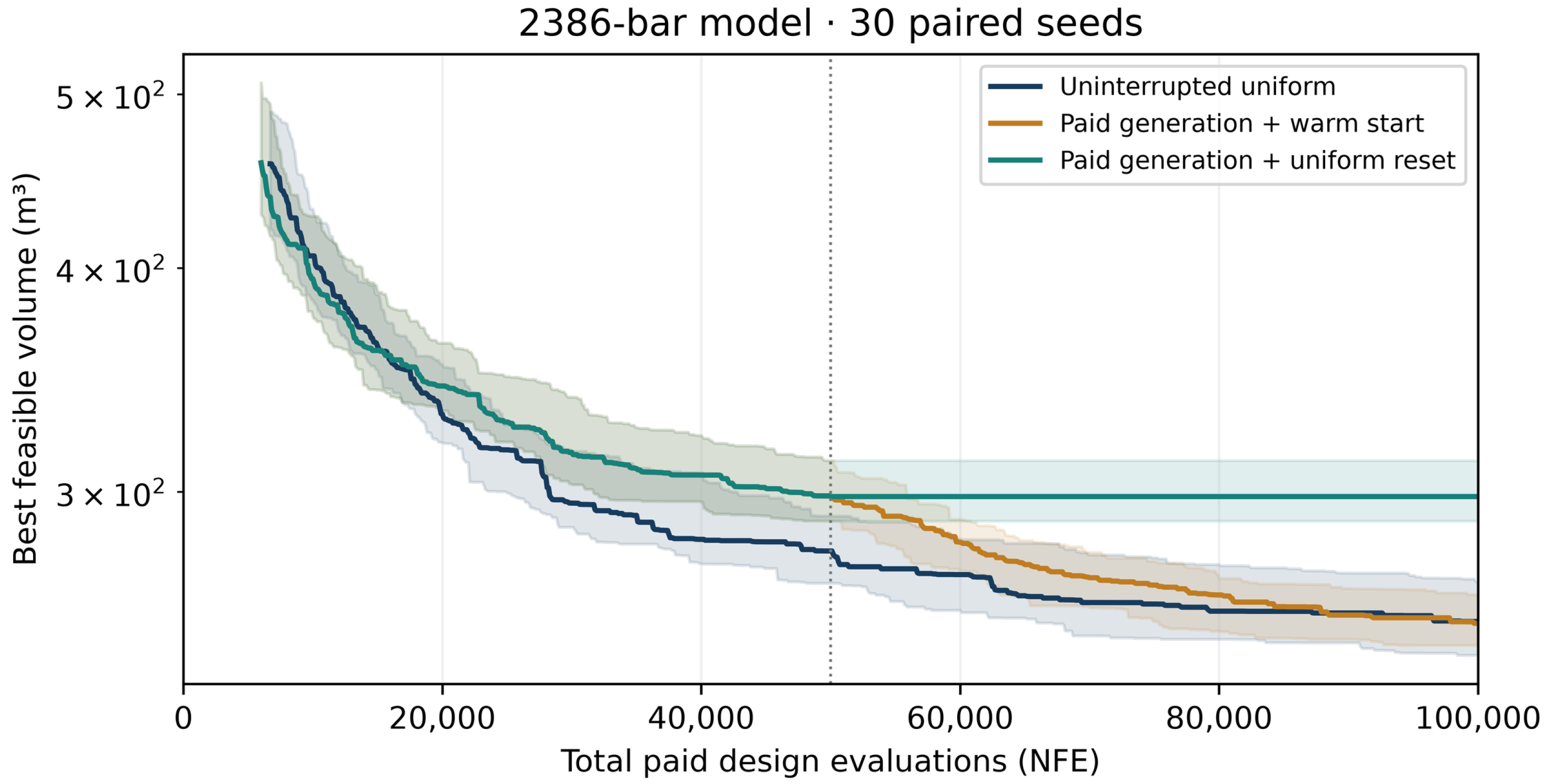
Paid warm starts improve the 200 bar mean by 400.679 kg relative to uninterrupted search, but this contrast does not meet the 5% threshold after six-comparison Holm adjustment (p = 0.06255). For 2386 bars, the mean difference is +0.624 m3 (Holm p = 0.95153), providing no evidence of improvement over uninterrupted search. Warm starts outperform the uniform reset control on both models (Holm p = 1.03 × 10⁻⁵ and 1.12 × 10⁻⁸), showing that preserving a generated elite helps under the tested reset protocol without establishing a general benefit of splitting a fixed budget.
Paired bootstrap intervals and two-sided Wilcoxon tests compare all three policy pairs on each model, with Holm adjustment across these six contrasts. Feasibility-first wins retain all thirty pairs. Targets of 11,600 kg and 200 m3 were declared before this additional study after inspecting earlier results; target access is consequently descriptive and post hoc relative to the original experiment. Targets do not change stopping or budgets. No inference about the full cost or reliability of the historical LATSS v2 archive follows from this controlled new study. Table 16 summarizes the additional SAP2000 checks of the best independently feasible design under each staged initialization policy for the 200 and 2386 bar models.
Table 16.
Additional SAP2000 checks of the best independently feasible design under each staged initialization policy.
All four selected staged policy designs satisfy the declared axial constraints recalculated from SAP2000 responses. Source models are preserved; the copies, readback records and saved response checks are supplied separately. These selected checks do not verify every initialization study vector or omitted structural limit states.
3.5. Literature-Assisted LATSS Series for the 200 Bar Model
A separate LATSS series for the static 200 bar model was initialized around the published JA section vector and small perturbations of that vector. Ten independent runs with seeds 13–22 used a population of 50 and a budget of 50,000 NFE. Each run comprises 49,999 search evaluations and one final repeat evaluation. All ten runs satisfied the FEM constraints. The best design was obtained with seed 22 and passed the recorded SAP2000 check. Table 17 summarizes the literature-assisted LATSS results for the 200 bar model and the verification results for the selected design.
Table 17.
Literature-assisted series for the 200 bar model and verification summary for the selected design.
Using the displayed mass values, the best literature-assisted design is 0.463684 kg (0.004015%) lighter than the published JA mass and 0.454172 kg (0.003932%) lighter than the local reanalysis of the same JA vector. These differences are interpreted as local improvement. The common JA initialization and low dispersion do not demonstrate general robustness to random starts. The area vector is given in Table A3, and statistics for other literature methods are provided in Appendix D.
3.6. LATSS v2 Archive-Selected Designs
LATSS v2 denotes a collection of the best recorded designs selected by screening the LATSS and earlier LASS archives. The label does not identify a new algorithm implementation or a rerun of the six-model experimental series. A total of 472 distinct designs that could be matched to source models were reevaluated under the current frozen model inputs; four additional warm-start designs were also checked. The selected results are listed in Table 18. The 200, 582, 942, and 2386 bar designs come from individual additional runs initialized from previously obtained good sections. The 1938 and 3586 bar designs are the best members of the existing 30-run series. Original algorithm names, seeds, and section vectors are retained in the source records. No new 30-run sample, mean, standard deviation, or success rate is derived from this collection, and the total costs of generating designs with different initialization histories are not equal.
Table 18.
LATSS v2 best-of-records selection under the frozen local protocols.
The additional runs for the 200, 582, 942, and 2386 bar models used seed 81008 and 100,000 NFE; population sizes were 50 for the first three models and 100 for the 2386 bar model. Their combined cost of 400,000 NFE is additional to the cost of obtaining the preceding designs. Recorded SAP2000 verification is available for the selected 1938 and 3586 bar designs, but no new SAP2000 checks were performed for the four additional designs. The 582 and 942 bar results belong to the earlier positive cubic denominator protocol, and the 2386 bar result uses the 80 mm displacement limit. The frozen 1938 and 3586 bar models use horizontal loads equal to one-tenth of the thesis values; these results cannot be interpreted as verified under the full thesis loading. Source-model matching is incomplete for the earlier LASS records of 19.565996 m3 for the 582 bar model and 20.261135 m3 for the 942 bar model. The earlier LATSS 942 bar design with 19.913842 m3 uses a geometry/group mapping different from the current model. These lower values are excluded from Table 18. In the additional sparse FEM capacity checks, the 582, 942, and 2386 bar archive vectors satisfied the corrected capacity equation and their local displacement limits; the 2386 bar archive vector did not satisfy the 50 mm limit. These checks do not change the statistical status of the archive selections.
4. Discussion
4.1. Interpretation of Utilization-Driven Search
The defining feature of LATSS is the link between candidate generation and demand-to-capacity information obtained from structural analysis. Highly utilized groups are more likely to be selected for growth, whereas groups with low utilization are selected more frequently for pruning. Although this mechanism has an engineering interpretation, the utilization ratios of a preceding design do not guarantee satisfaction of the constraints in a new design. Reanalysis of every offspring and a separate feasibility criterion are therefore integral to the method.
Performing discrete sizing operations on physical areas rather than catalog indices avoids an artificial assumption that capacity follows index order. Retaining the identities of equal area sections and using their actual minimum radii of gyration are important. In the SAP2000 copies, the R22/R33 transfer was corrected to match the catalog axes, while areas, second moments of area, frozen minimum radii of gyration, and the 10−7 transfer tolerance were unchanged. Transfer consistency does not, however, establish exact equivalence between catalog versions and those used in the literature.
4.2. Initialization, Evaluation Counts, and Comparison Fairness
The initialization distribution can affect the solution regions reached by metaheuristics and the variability across independent runs [43]. Accordingly, the main independent start series, the series initialized around the literature JA design, and the additional runs initialized from previously obtained good designs are evaluated separately. Table 18 presents archive designs selected from different initialization histories; it is not a controlled experiment isolating the effect of initialization strategy. In particular, the difference observed for the 2386 bar model suggests that access to this design region from independent starts should be improved. A single additional run is nevertheless insufficient to characterize initialization sensitivity statistically.
The six-model comparison favors LATSS on four defined models and DE on the 200 and 2386 bar models. Restart-equipped JAYA/TLBO reduce the imbalance in recovery mechanisms; they do not reproduce all published enhancements or a tuned baseline. LATSS still has lower best and mean tower masses than these tested variants. Physical-area projection and catalog index rounding remain different representation choices. The simple utilization heuristic is strong on the stress-only 200 bar problem but has low success on 942 bars, showing that neither complexity nor the tree analogy establishes general superiority.
NFE, NSA, and elapsed time are different measures of computational cost. Literature analysis counts at best-design attainment are not equivalent to the total evaluation budgets assigned here. Similarly, first attainment of a run’s final best design does not measure the cost of reaching a common target. Without controlled hardware and process conditions, wall-clock rankings would exceed the evidence available for computational cost comparisons.
Figure 25 shows the recorded mean elapsed times per model in the main 30-run series. Each run comprises 100,000 NFE. The means for the 200, 582, 942, 1938, 2386, and 3586 bar models are 241.4, 543.8, 709.3, 1213.5, 2284.8, and 2804.8 s, respectively. Because concurrent process loads and hardware conditions were not held constant across experiments, the figure is descriptive; it demonstrates neither interalgorithm speed superiority nor a scaling law based solely on member count.
Figure 25.
Recorded mean elapsed time per 100,000-NFE run across 30 independent LATSS runs for each local model. Wall-clock times are descriptive and were not measured under controlled hardware and concurrent process conditions.
4.3. Model Equivalence and Structural Validity
Published algorithm results, local reanalyses, and the current independent LATSS runs constitute different types of evidence. A literature design reported with a lower volume may violate constraints in a local reanalysis because of differences in inputs, catalogs, or capacity interpretation. Such a result alone does not establish failure of the literature algorithm. The literature values in Appendix D are not presented as competitor runs performed anew in this study.
The horizontal nodal magnitudes 667.2 and 444.8 N agree with the specified chapter [34], whereas the thesis [35] uses different values. Therefore, the earlier blanket statement that the models used one-tenth of every source load was inaccurate. The 1938 cut-plane model remains a local topology/support adaptation. Corrected 582/942 optimization now changes search trajectories and distributions. For 2386, the source-aligned 80 mm discrete context [12] and the additional 50 mm local discrete study must both remain distinct from the continuous area case [36]. Catalog and grouping equivalence is not certified by matching one displacement bound.
Applying these results to a real tower project would require assessment of connections, fabrication, foundations, site-specific wind and other project loads, and second-order behavior. This data set does not constitute a site-specific engineering project. Feasibility in a linear axial model cannot replace broader design objectives such as safety against imperfections or member loss and assessment of post-buckling behavior [44,45].
4.4. Limitations and Future Research
The equal budget ablations quantify removal effects only within the tested configurations. They do not estimate all interactions, retune the remaining operators, or identify a unique optimal schedule. Uniform weighting changes probabilities within the same eligible group sets; it does not remove utilization thresholds or growth magnitudes. Fixed pruning can improve some models, and restart removal sometimes improves results. Broader parameter sensitivity, factorial experiments, and additional problem families are needed before generalizing component contributions.
The cost-accounted initialization study in Section 3.4.8 covers two frozen local models and freshly generated same-seed designs. It does not recover the unknown generation cost of historical archive selections, which remain descriptive. Warm versus uniform reset policies isolate elite injection under a common phase reset; comparison against uninterrupted search also changes phase allocation. Tightened acceptance thresholds and fixed vector displacement reserves do not constitute reoptimization under engineering margins. The linear axial checks omit connections, local and torsional buckling, imperfections, and second-order or dynamic behavior. New SAP2000 checks cover ten earlier revision selections and four initialization study selections, not every run. No public repository DOI is claimed. Source-equivalent catalog and topology studies remain necessary for broader literature rankings.
5. Conclusions
The revised primary LATSS sample contains 30 independent uniform start runs per model, with corrected Compression equation searches used for 582/942. All primary designs satisfy their defined axial constraints. The 1200 additional revision runs, and 120 million NFE separately test the corrected equation, component removals, a simple resizing heuristic, restart-equipped tower baselines, and the 50 mm displacement case. Together with the original controlled series, 1680 completed runs and 168 million NFE are retained without pooling incompatible protocols. The separate initialization experiment contributes nine million physical NFE, bringing the retained controlled-evaluation total to 177 million; shared preparation stages are counted only once.
Primary best masses remain 12,267.383, 171,898.150 and 561,361.170 kg for 200, 1938 and 3586 bars. Corrected best volumes are 21.002 and 23.102 m3 for 582 and 942 bars; the 2386 primary 80 mm result remains 229.303 m3. At 50 mm, LATSS and DE obtain 430.422 and 406.508 m3. Ten selected new designs pass SAP2000 response and model-constraint checks, with maximum normalized displacement disagreement below 2.90 × 10⁻¹⁰. This does not certify complete modern steel code compliance.
LATSS has lower best and mean objectives than the tested DE implementation on four local models, while DE is better on the 200 and 2386 bar models. LATSS also outperforms the implemented restart-equipped JAYA/TLBO tower baselines in best and mean mass. These statements are supported by paired records, explicit success counts, and conditional statistics. Basic TLBO boundary disagreements remain visible in the original series; they are not erased by reporting the separate enhanced experiments.
Separate warm-start searches showed that lower objective values than those in the main series could be reached. The LATSS v2 archive selections achieved 11,549.1212 kg for the 200 bar model and 20.7522, 20.9647, and 186.7827 m3 for the 582, 942, and 2386 bar models, respectively. These values do not represent a new equal budget sample of 30 runs. Initial-design generation costs differ, and new SAP2000 checks of the four additional designs have not been completed. The archive selection is therefore kept separate from the main-series means, standard deviations, and success rates.
Mutation has a substantial favorable removal contrast on several larger models, but staged pruning and restart do not benefit every problem. The simple resizing heuristic reaches lower conditional masses on the stress-only 200 bar case, whereas it verifies only 8/30 final 942 bar designs. These mixed findings support a bounded, model-dependent interpretation of LATSS. Improving access to good regions from independent starts, clarifying full source equivalence, and testing omitted engineering limit states remain priorities.
Supplementary Materials
The following are available online at https://www.mdpi.com/article/10.3390/buildings16214328/s1. Reproduction_Data.zip: Reproduction data supporting the analyses reported in this study.
Funding
This research received no external funding.
Data Availability Statement
The SAP2000 model for each case study is available from the corresponding author upon request for reproduction purposes.
Conflicts of Interest
The author declares no conflicts of interest.
Abbreviations
The following abbreviations are used in this manuscript.
| Term | Description |
| LATSS | Probabilistic Load-Adaptive Tree-Inspired Section Selection |
| FEM | Finite element method |
| NFE | Number of candidate design evaluations |
| NSA | Number of structural right-hand side solutions for the load cases |
| SD | Sample standard deviation |
| NOE | Number of members with stress-check exceedance above tolerance |
| AISC | American Institute of Steel Construction |
| CVσ/CVU | Maximum positive normalized stress/displacement exceedance (%) |
| CVf | Coefficient of variation in the objective; 100 × SD/mean |
| TLBO | Teaching–learning-based optimization |
| ASD | Allowable stress design |
| VPS | Vibrating particles system |
| N/A | Measure undefined or data unavailable |
Appendix A. Unit Conversions and Model Constraints
This appendix summarizes the model-specific limits associated with the common formulation in the main text. The distinction between mass and volume objectives is retained. Unit conversions use 1 in = 0.0254 m, 1 lbm = 0.45359237 kg, and 1 kip = 4.4482216152605 kN. The density of 0.283 lb/in3 in the static 200 bar problem is interpreted as lbm/in3 for mass calculations. A general treatment of constrained structural optimization is provided in [46].
Appendix A.1. Stress, Slenderness, and Displacement
Member slenderness is calculated using Equation (A1), where K is the effective length factor and rmin is the minimum radius of gyration of the section. K = 1 is used for the 582-, 942-, and 2386-bar models. Sign-dependent capacity checks use the tensile capacity for tensile stress and the compressive capacity for the absolute value of compressive stress.
For the 582-, 942-, and 2386 bar models, the allowable tensile stress on the gross section is σt,allow = 0.60Fy, based on AISC–ASD (1989), Section D1 [28]. Critical slenderness is defined by Equation (A2). Equations (A3) and (A4) reproduce expressions E2-1 and E2-2, respectively, from Section E2. E and Fy must be expressed in the same stress units.
Equation (A3) uses the negative cubic term of the AISC–ASD (1989) reference [28]. It is used during every evaluation of the corrected 582/942 experiments, not merely in final vector checking. Original positive cubic histories are retained separately for sensitivity. The negative expression increases the inelastic allowable stress for fixed inputs; because utilization guides proposals, its influence extends to subsequent search trajectories. Modern code diagnostics remain incomplete code checks.
The tension limit λ ≤ 300 is active in all three discrete models. In compression, λ ≤ 200 is a separate acceptance criterion for the 582 and 942 bar models; for the 2386 bar model it is a recommended value rather than an independent rejection criterion. Under AISC–ASD (1989), Section B7, the allowable stress cannot exceed the value from Equation (A4) when compression slenderness exceeds 200 [28]. Equation (A5) defines the constraint function for a symmetric displacement limit.
Appendix A.2. Compression Capacity of the Continuous Section Towers
For the continuous towers, Equation (A6) is consistent with mean-diameter ratio Dm/t = 100. With outer and inner diameters Do = 101t and Di = 99t, area A = 100πt2 and radius of gyration r2 = (Do2 + Di2)/16 = (10,001/8)t2 = 100.01A/(8π). Substituting this into the pinned Euler stress π2Er2/L2 gives Equation (A6). Outer-diameter ratio Do/t = 100 would instead give coefficient 99.0101 and is not the convention consistent with the recorded search formula. No compression yield cap or full tube-local-buckling check is inferred from this elastic idealization.
The area bounds for these two models are 0.1 ≤ Ag ≤ 200 in2, equivalently 0.64516 ≤ Ag ≤ 1290.32 cm2. The local tensile limit is 40 ksi, and the displacement limit is 406.4 mm. All conditions are checked for three separate load cases; LC1–LC3 are not combined into a single total load combination.
Appendix A.3. Specific Definition of the Static 200 Bar Model
Only stress constraints and lower area bounds are specified in the source definition of the static 200 bar problem [7]. Checking the absolute stress of every member under three load cases gives 600 ratios. Counting tension and compression as separate inequalities gives 1200 stress inequalities. Because no upper area bound is given in the literature, the local 20 in2 cap must be treated as a separate search choice.
σallow = 10 000 psi = 68.947572932 MPa
Ag ≥ 0.1 in2 = 6.4516 × 10⁻⁵ m2, g = 1,…,29
Table A1.
Recorded search constraints and separate corrected capacity checks.
Compression capacity in the 1938- and 3586 bar models depends on member length and area. The absence of a separately specified slenderness limit does not imply the absence of a buckling check. Similarly, the reported Umax for the 200 bar model, which has no displacement limit, is not converted into a new acceptance criterion.
Appendix B. Design Groups and Section Vectors
The following tables report the group assignments generated from the stored local models and the LATSS section vectors obtained in this study. Each vector is identified by its model and seed. The detailed 200-member area vector is the JA-assisted seed-22 design and is kept separate from the uniformly initialized series. Published benchmark definitions remain attributed in the text; full third-party section tables and graph-digitized approximate areas are omitted.
Appendix B.1. 200 Bar Truss
Table A2.
Local 200-member model group assignments generated from stored member identifiers and group data; n is the member count. Problem definition context: [7,46].
Table A3.
Group sections of the source-assisted LATSS design for the 200-member model (seed 22); member counts are derived from the stored model mapping.
Appendix B.2. 582 Bar Tower
Table A4.
Local 582-member model group assignments generated from stored member identifiers and group data; n is the member count. Problem definition context: [11].
Table A5.
Group sections of the corrected expression LATSS design for the 582-member model (seed 3); member counts are derived from the stored model mapping.
Appendix B.3. 942 Bar Tower
Table A6.
Local 942-member model group assignments generated from stored member identifiers and group data; n is the member count. Problem definition context: [11].
Table A7.
Group sections of the corrected expression LATSS design for the 942-member model (seed 17); member counts are derived from the stored model mapping.
Appendix B.4. 1938 and 3586 Bar Towers
Figure A1.
Published member-group details for the 1938- and 3586 bar reference towers. Panels (a–g) cover the upper tower; panels (h,i) show the additional lower transition and segment. Adapted from Degertekin et al. [10], Appendix A, Figure A1, under CC BY 4.0 (https://creativecommons.org/licenses/by/4.0/). Redrawn from the source schematic for improved legibility. Colors distinguish member groups within each panel, with group numbers identified in the panel-specific keys. Colors do not represent stress or displacement values.The local computational group assignments are reported separately in this appendix.
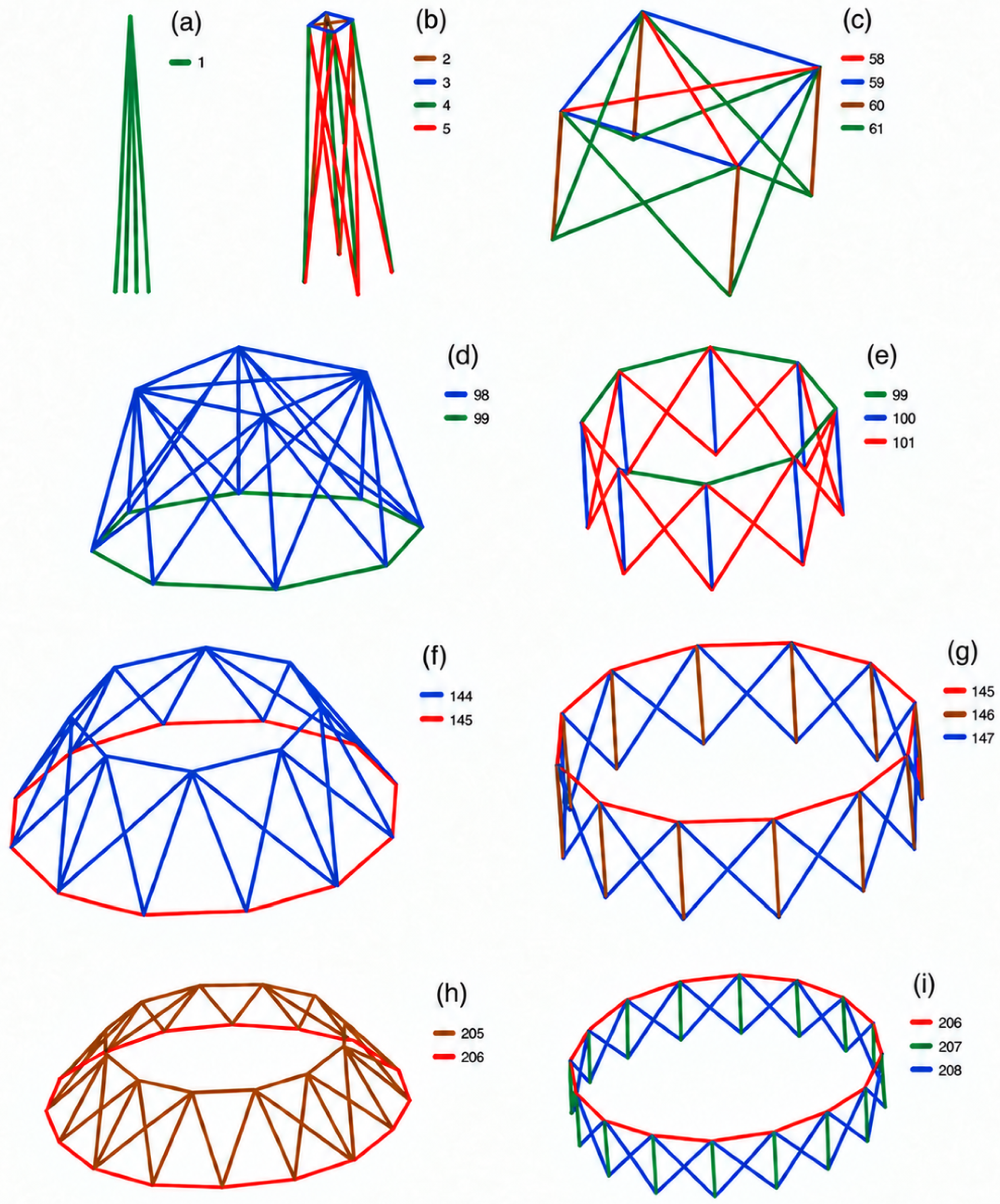
Table A8.
Group areas of the selected local 1938-member LATSS design (seed 28); all areas are in in2.
Table A9.
Group areas of the selected local 3586-member LATSS design (seed 16); all areas are in in2.
Appendix B.5. 2386 Bar Tower
Table A10.
The 220 W profiles of the local 2386-member LATSS design (seed 12); n is the number of members assigned to the group.
Appendix C. Nodal Loads Used in This Study
The force vector in Table A11 is applied separately to every node in the stated set. External forces at unlisted nodes are zero. Ranges include both endpoints and all intervening integers. Node numbers are the node_names identifiers in the frozen model; the N prefix is omitted for the 200- and 582 bar models. No external loads are assigned to support nodes 470–481 in the 1938 bar model. Loads on the retained free nodes of the 3586 bar tower were transferred unchanged to the upper-tower model.
The vertical direction is Y for the 200 bar model and Z for the towers. LC1–LC3 are separate cases for the two large towers. The 1938 bar upper tower retains loads on free nodes and has a translation-restrained cut-plane base. The horizontal nodal magnitudes agree with [34] but are one tenth of the corresponding values in the thesis [35]. These source-specific loading statements do not remove the upper-tower topology and support adaptation.
Table A11.
Node sets and loads per node (kN/node).
Appendix D. Literature Comparison Tables
The following tables are the authors’ own compilations of selected numerical results and problem definitions. Published data are identified explicitly by their source; they are not competitor runs carried out in this study. Full literature section vectors and copied source-table layouts are omitted. Reported analysis counts are preserved as source-specific measures and must not be treated as budgets identical to the local NFE. Controlled comparisons are reported in the main text.
Table A12.
Author’s compilation of best masses and reported computational counts for the 200-member problem. Data from [7] and this study; method citations identify the underlying algorithms.
Table A13.
Author’s compilation of selected 582-member objective data in m3 and source-specific computational counts. Data from [11] and this study; local and published protocols are not assumed equivalent.
Table A14.
Author’s compilation of selected 942-member objective data in m3 and source-specific computational counts. Data from [11] and this study; local and published protocols are not assumed equivalent.
Table A15.
Author’s compilation of selected best masses for the 1938-member tower context and the local adapted LATSS problem. Data from [10] and this study; masses are in t.
Table A16.
Author’s compilation of selected best masses for the 3586-member tower context and the locally adapted LATSS problem. Data from [10] and this study; masses are in t.
Table A17.
Author’s compilation of selected 2386-member objective data in m3 and source-specific computational counts. Data from [13] and this study; local and published protocols are not assumed equivalent.
Table A18.
Author’s compilation of the distinct 2386-member formulations and their best reported objectives. Data from [36] and this study; objectives with different units and feasible regions are not ranked.
Appendix E. SAP2000 Responses of Selected Designs
These figures show selected SAP2000 responses. The 582/942 panels use the corrected search designs and newly returned SAP2000 fields; the 1938/3586 and 80 mm 2386 panels retain the earlier primary designs. Deformation amplification is for visualization. Separate verification records document the ten newly selected comparator and sensitivity designs. Response agreement and axial acceptance do not cover every steel failure mode.
Appendix E.1. 582-Bar Model
Figure A2.
Reopened SAP2000 deformation and axial-stress fields for corrected expression LATSS seed 3 of the 582 bar model. The plotted deformation scale is indicated in the figure.
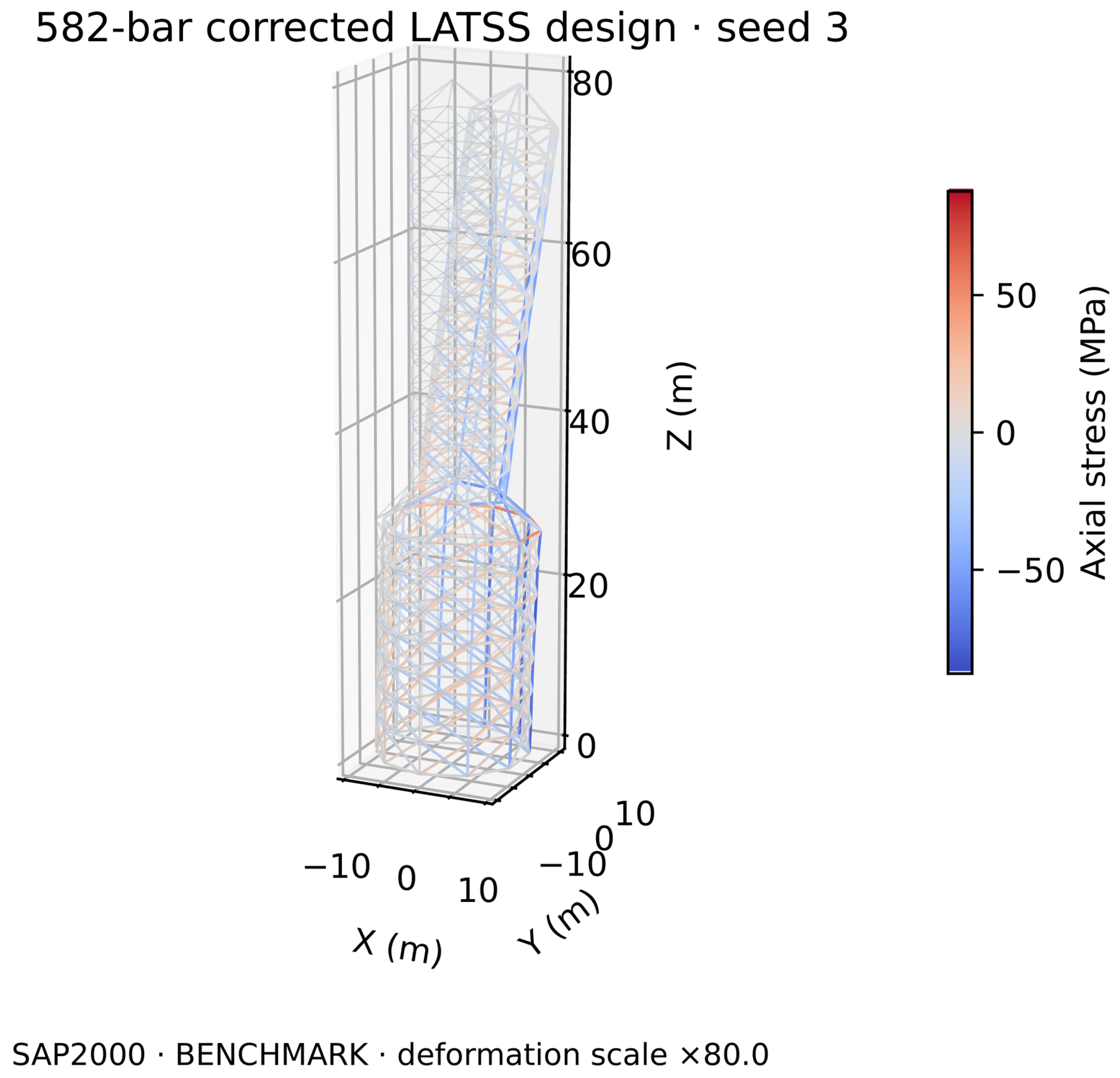
Figure A3.
Reopened SAP2000 displacement components and axial stresses for corrected expression LATSS seed 3 of the 582 bar model.
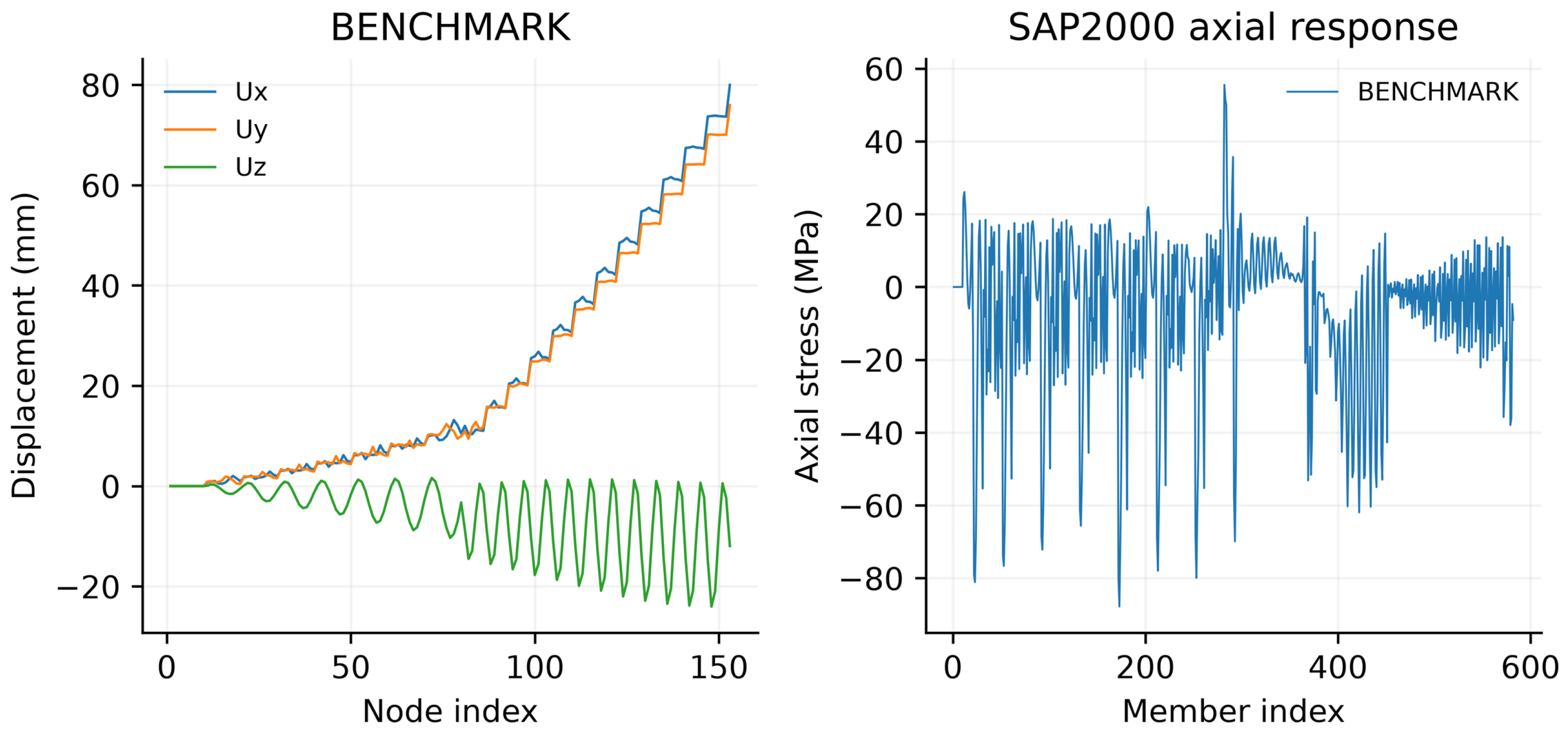
Appendix E.2. 942-Bar Model
Figure A4.
Reopened SAP2000 deformation and axial-stress fields for corrected expression LATSS seed 17 of the 942 bar model. The plotted deformation scale is indicated in the figure.
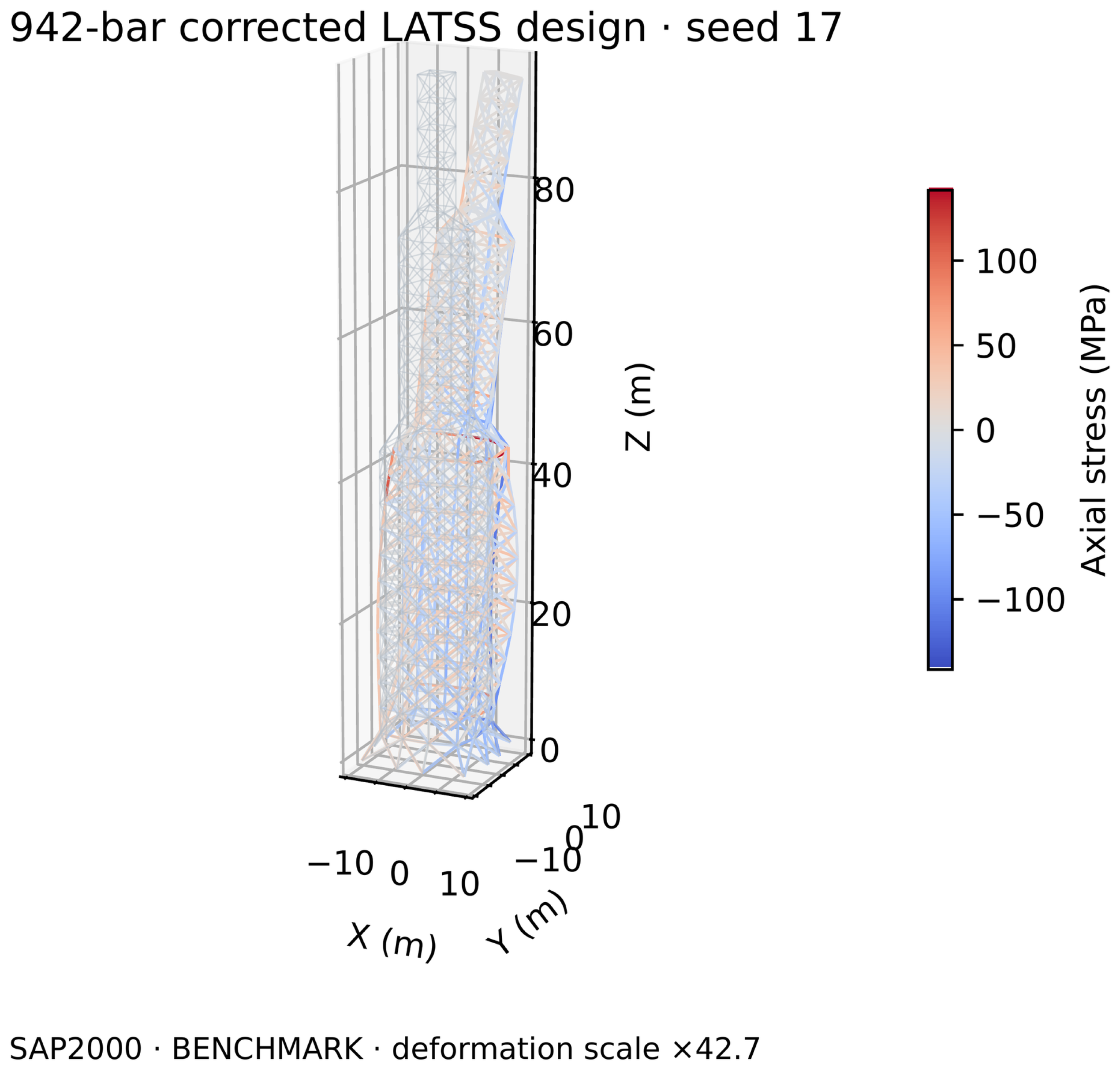
Figure A5.
Reopened SAP2000 displacement components and axial stresses for corrected expression LATSS seed 17 of the 942 bar model.
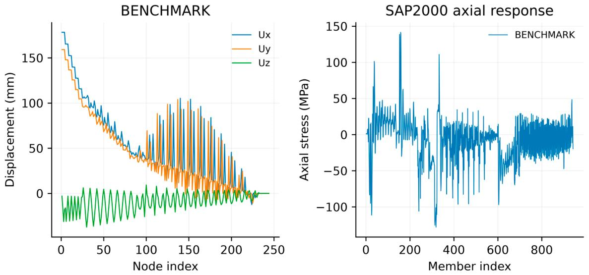
Appendix E.3. 1938-Bar Model
Figure A6.
Deformation and axial stresses of the best 1938 bar design (seed 28) under LC2. Deformation scale: ×49.1.
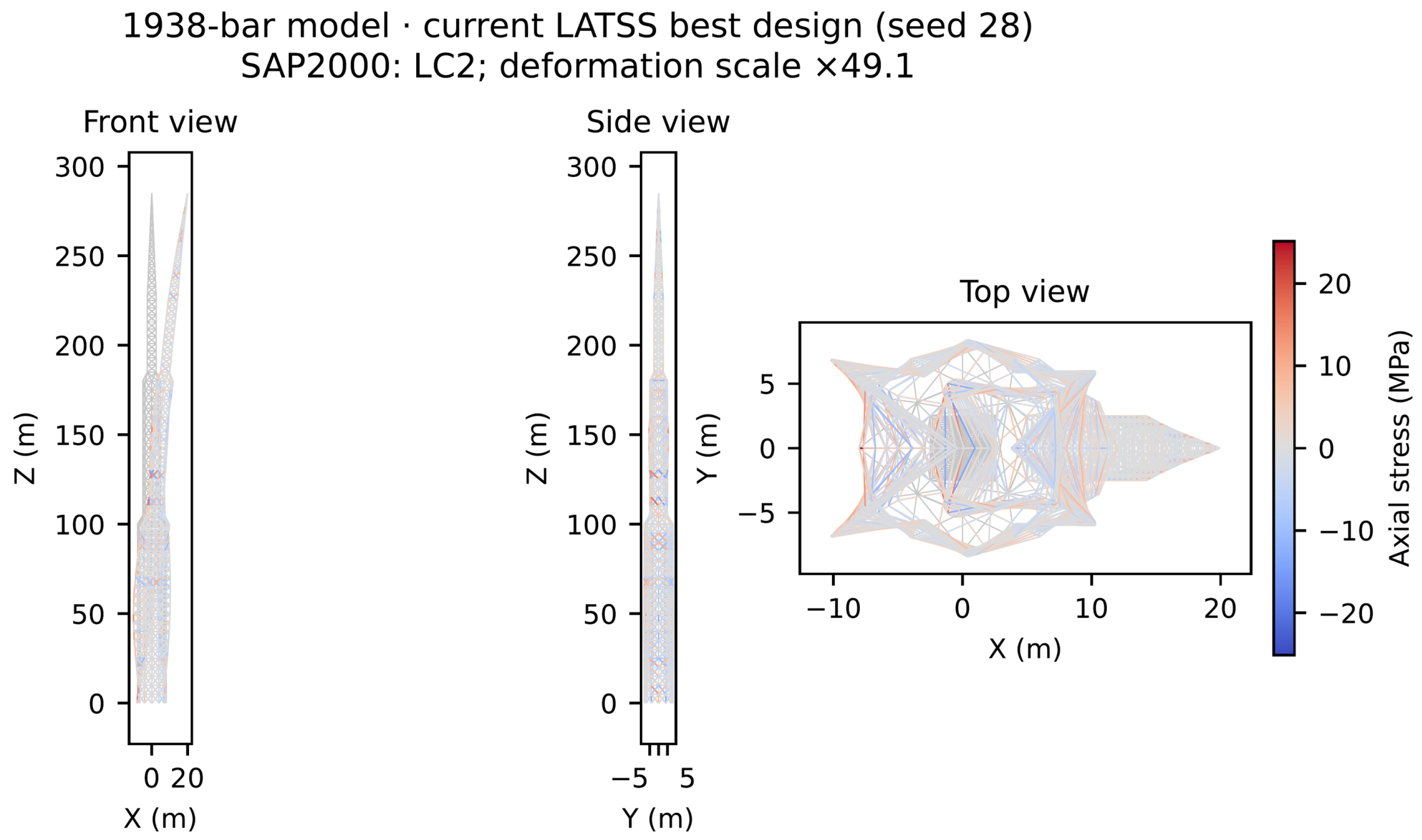
Figure A7.
Displacement components under LC2 and member axial stresses for each load case of the 1938 bar design (seed 28).
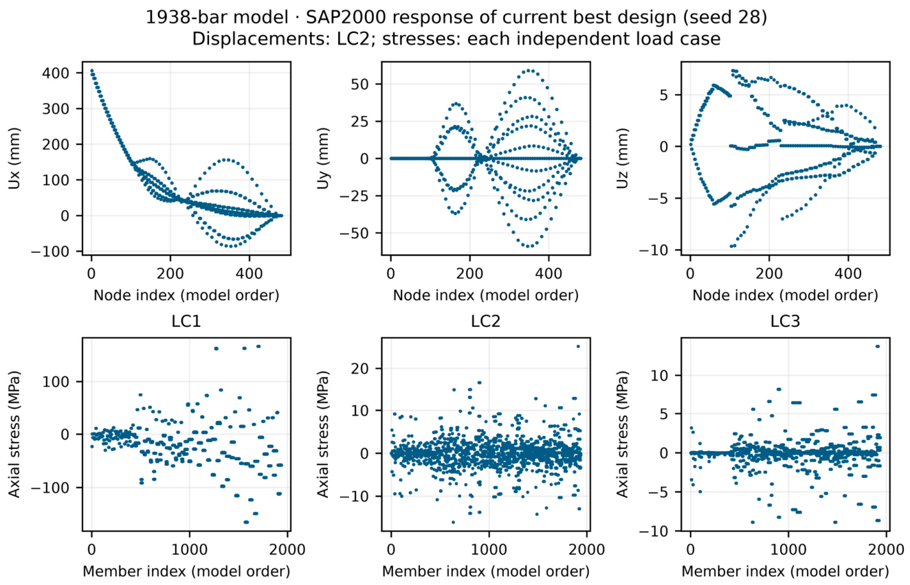
Appendix E.4. 3586 Bar Model
Figure A8.
Deformation and axial stresses of the best 3586 bar design (seed 16) under LC2. Deformation scale: ×71.5.
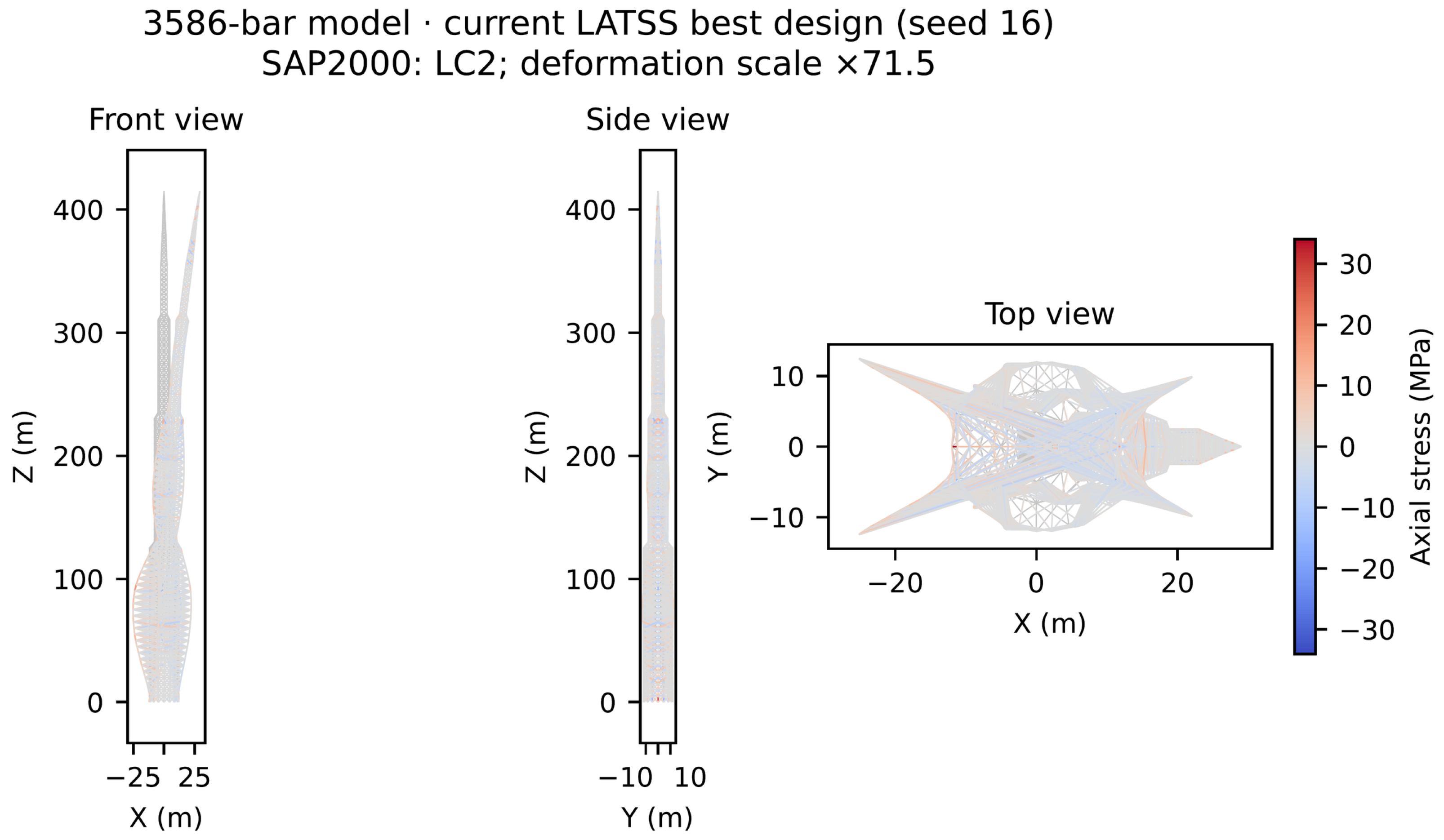
Figure A9.
Displacement components under LC2 and member axial stresses for each load case of the 3586 bar design (seed 16).
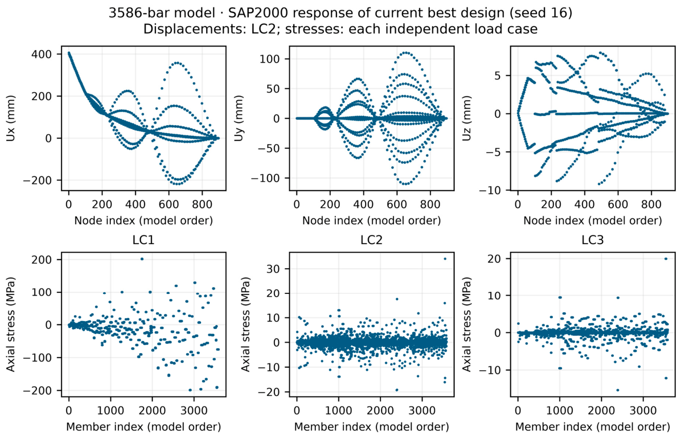
Appendix E.5. 2386-Bar Model
Figure A10.
Deformation and axial stresses of the best 2386 bar design (seed 12) under PAPER_COMBINED. Deformation scale: ×72.3.
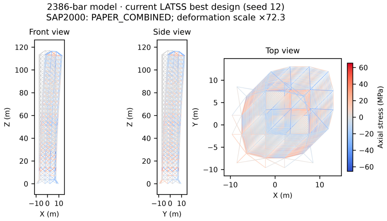
Figure A11.
Displacement components under PAPER_COMBINED and member axial stresses for each load case of the 2386 bar design (seed 12).
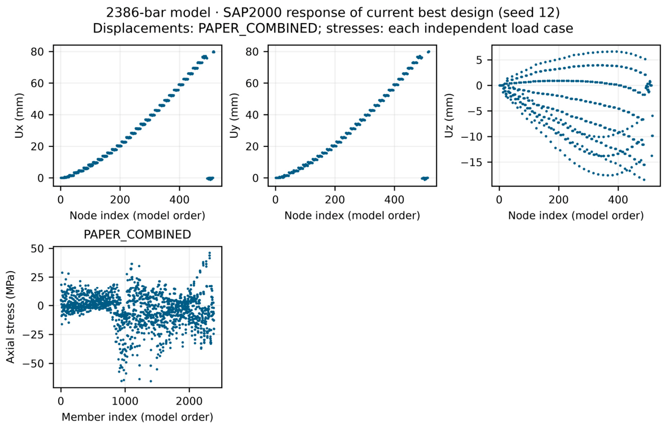
References
- Hasançebi, O.; Çarbaş, S.; Doğan, E.; Erdal, F.; Saka, M.P. Performance evaluation of metaheuristic search techniques in the optimum design of real size pin jointed structures. Comput. Struct. 2009, 87, 284–302. [Google Scholar] [CrossRef] [Scilit]
- Brütting, J.; Senatore, G.; Fivet, C. MILP-based discrete sizing and topology optimization of truss structures: New formulation and benchmarking. Struct. Multidiscipl. Optim. 2022, 65, 277. [Google Scholar] [CrossRef] [Scilit]
- Storn, R.; Price, K. Differential Evolution—A simple and efficient heuristic for global optimization over continuous spaces. J. Glob. Optim. 1997, 11, 341–359. [Google Scholar] [CrossRef] [Scilit]
- Geem, Z.W.; Kim, J.H.; Loganathan, G.V. A new heuristic optimization algorithm: Harmony Search. Simulation 2001, 76, 60–68. [Google Scholar] [CrossRef] [Scilit]
- Rao, R.V. Jaya: A simple and new optimization algorithm for solving constrained and unconstrained optimization problems. Int. J. Ind. Eng. Comput. 2016, 7, 19–34. [Google Scholar] [CrossRef] [Scilit]
- Rao, R.V.; Savsani, V.J.; Vakharia, D.P. Teaching–learning-based optimization: A novel method for constrained mechanical design optimization problems. Comput.-Aided Des. 2011, 43, 303–315. [Google Scholar] [CrossRef] [Scilit]
- Degertekin, S.O.; Lamberti, L.; Ugur, I.B. Sizing, layout and topology design optimization of truss structures using the Jaya algorithm. Appl. Soft Comput. 2018, 70, 903–928. [Google Scholar] [CrossRef] [Scilit]
- Degertekin, S.O.; Lamberti, L.; Ugur, I.B. Discrete sizing/layout/topology optimization of truss structures with an advanced Jaya algorithm. Appl. Soft Comput. 2019, 79, 363–390. [Google Scholar] [CrossRef] [Scilit]
- Lamberti, L. An efficient simulated annealing algorithm for design optimization of truss structures. Comput. Struct. 2008, 86, 1936–1953. [Google Scholar] [CrossRef] [Scilit]
- Degertekin, S.O.; Minooei, M.; Santoro, L.; Trentadue, B.; Lamberti, L. Large-scale truss-sizing optimization with enhanced hybrid HS algorithm. Appl. Sci. 2021, 11, 3270. [Google Scholar] [CrossRef] [Scilit]
- Kaveh, A.; Raissi Dehkordi, M.; Shaghaghian, A.H. Stellar flickering optimization: A probabilistic approach with adaptive success history for large scale numerical optimization and design of real-sized structures. Comput. Struct. 2026, 329, 108291. [Google Scholar] [CrossRef] [Scilit]
- Kaveh, A.; Ilchi Ghazaan, M. Optimum design of large-scale truss towers using cascade optimization. Acta Mech. 2016, 227, 2645–2656. [Google Scholar] [CrossRef] [Scilit]
- Kaveh, A.; Ilchi Ghazaan, M. MATLAB code for vibrating particles system algorithm. Int. J. Optim. Civ. Eng. 2017, 7, 355–366. Available online: https://ijoce.iust.ac.ir/article-1-302-en.html (accessed on 20 October 2026).
- Fakhimi, R.; Shahabsafa, M.; Lei, W.; He, S.; Martins, J.R.R.A.; Terlaky, T.; Zuluaga, L.F. Discrete multi-load truss sizing optimization: Model analysis and computational experiments. Optim. Eng. 2022, 23, 1559–1585. [Google Scholar] [CrossRef] [Scilit]
- El Bouzouiki, M.; Sedaghati, R.; Stiharu, I. A non-uniform cellular automata framework for topology and sizing optimization of truss structures subjected to stress and displacement constraints. Comput. Struct. 2021, 242, 106394. [Google Scholar] [CrossRef] [Scilit]
- Ugur, I.B.; Aydemir, S.B.; Kutlu Onay, F. Optimum design of high-dimensional truss structures using the bonobo optimizer with inertia weight strategies. Eng. Optim. 2026, 58, 1973–2010. [Google Scholar] [CrossRef] [Scilit]
- Degertekin, S.O.; Tutar, H. Performance-based optimum seismic design of planar steel frames using the Jaya algorithm. In Proceedings of the 4th Eurasian Conference on Civil and Environmental Engineering, Istanbul, Turkey, 2019; Sahinkaya, S., Ed.; Gelisim University: Istanbul, Turkey, 2019; pp. 1315–1326. [Google Scholar]
- Degertekin, S.O.; Tutar, H.; Lamberti, L. Performance-based optimum seismic design of steel frames using the teaching–learning-based optimization. In Proceedings of the Fifth International Conference on Soft Computing and Optimisation in Civil, Structural and Environmental Engineering, Riva del Garda, Italy, 2019; Topping, B.H.V., Logo, J., Eds.; Elsevier: Amsterdam, The Netherlands, 2019. [Google Scholar]
- Degertekin, S.O.; Tutar, H.; Lamberti, L. School-based optimization for performance-based optimum seismic design of steel frames. Eng. Comput. 2021, 37, 3283–3297. [Google Scholar] [CrossRef] [Scilit]
- Degertekin, S.O.; Tutar, H. Optimized seismic design of planar and spatial steel frames using the hybrid learning based jaya algorithm. Adv. Eng. Softw. 2022, 171, 103172. [Google Scholar] [CrossRef] [Scilit]
- Tutar, H. Comparative Analysis of Performance-Based Optimal Seismic Design of Planar Steel Frames Using the Multi-Class MC-TLBO Algorithm. Mus. Alparslan Univ. J. Sci. 2025, 13, 150–164. (In Turkish) [Google Scholar] [CrossRef] [Scilit]
- Wang, Y.; Chen, B.; Dai, P.; Chen, Y.; Sun, Y.; Song, Y.; Lim, J.B.P. Localized loading behaviour of perforated QN1803 high-strength stainless steel welded plate girders. J. Constr. Steel Res. 2025, 235, 109907. [Google Scholar] [CrossRef] [Scilit]
- Ye, Q.; Nie, H.; Chen, B.; Wang, Y.; Lu, P.; Dai, P.; Hai, L. Local buckling behaviour of welded stainless steel I-beams with perforated webs. Thin-Walled Struct. 2025, 212, 113201. [Google Scholar] [CrossRef] [Scilit]
- Talpur, S.A.; Thansirichaisree, P.; Poovarodom, N.; Mohamad, H.; Zhou, M.; Ejaz, A.; Hussain, Q.; Saingam, P. Machine learning approach to predict the strength of concrete confined with sustainable natural FRP composites. Compos. Part C Open Access 2024, 14, 100466. [Google Scholar] [CrossRef] [Scilit]
- Aranha, C.; Camacho Villalón, C.L.; Campelo, F.; Dorigo, M.; Ruiz, R.; Sevaux, M.; Sörensen, K.; Stützle, T. Metaphor-based metaheuristics, a call for action: The elephant in the room. Swarm Intell. 2022, 16, 1–6. [Google Scholar] [CrossRef] [Scilit]
- Del Ser, J.; Osaba, E.; Molina, D.; Yang, X.S.; Salcedo-Sanz, S.; Camacho, D.; Das, S.; Suganthan, P.N.; Coello Coello, C.A.; Herrera, F. Bio-inspired computation: Where we stand and what’s next. Swarm Evol. Comput. 2019, 48, 220–250. [Google Scholar] [CrossRef] [Scilit]
- Wolpert, D.H.; Macready, W.G. No free lunch theorems for optimization. IEEE Trans. Evol. Comput. 1997, 1, 67–82. [Google Scholar] [CrossRef] [Scilit]
- American Institute of Steel Construction (AISC). Specification for Structural Steel Buildings—Allowable Stress Design and Plastic Design, June 1, 1989. In Manual of Steel Construction—Allowable Stress Design, 9th ed.; AISC: Chicago, IL, USA, 1989. [Google Scholar]
- Deb, K. An efficient constraint handling method for genetic algorithms. Comput. Methods Appl. Mech. Eng. 2000, 186, 311–338. [Google Scholar] [CrossRef] [Scilit]
- Telewski, F.W. A unified hypothesis of mechanoperception in plants. Am. J. Bot. 2006, 93, 1466–1476. [Google Scholar] [CrossRef] [Scilit] [PubMed]
- Du, S.; Yamamoto, F. An overview of the biology of reaction wood formation. J. Integr. Plant Biol. 2007, 49, 131–143. [Google Scholar] [CrossRef] [Scilit]
- Deb, K.; Deb, D. Analyzing Mutation Schemes for Real-Parameter Genetic Algorithms. KanGAL Report 2012016. 2012. Available online: https://www.egr.msu.edu/~kdeb/papers/k2012016.pdf (accessed on 20 October 2026).
- DEAP Project. deap.tools.mutation: mutPolynomialBounded. Available online: https://deap.readthedocs.io/en/master/_modules/deap/tools/mutation.html (accessed on 9 October 2026).
- Lamberti, L.; Pappalettere, C. Truss weight minimization using hybrid harmony search and Big Bang–Big Crunch algorithms. In Metaheuristic Applications in Structures and Infrastructures; Chapter 9; Elsevier: Amsterdam, The Netherlands, 2013; pp. 207–240. [Google Scholar] [CrossRef] [Scilit]
- Minooei Mazloom, S.M. Design Optimization of Large-Scale Structures with Advanced Meta-Heuristic Methods. Ph.D. Thesis, Politecnico di Bari, Bari, Italy, 2022. Available online: https://tesidottorato.depositolegale.it/handle/20.500.14242/64365 (accessed on 20 October 2026).
- Shahrouzi, M.; Khavaninzadeh, N.; Jahanbakhsh, A. Jaya algorithm with passive congregation for design of structures with diagonal members. Int. J. Optim. Civ. Eng. 2020, 10, 277–294. Available online: https://ijoce.iust.ac.ir/article-1-434-en.html (accessed on 20 October 2026).
- Degertekin, S.O.; Yalcin Bayar, G.; Lamberti, L. Parameter free Jaya algorithm for truss sizing-layout optimization under natural frequency constraints. Comput. Struct. 2021, 245, 106461. [Google Scholar] [CrossRef] [Scilit]
- Moez, H.; Kaveh, A.; Taghizadieh, N. Natural forest regeneration algorithm for optimum design of truss structures with continuous and discrete variables. Period. Polytech. Civ. Eng. 2016, 60, 257–267. [Google Scholar] [CrossRef] [Scilit]
- Bodalal, R.; Shuaeib, F. Marine predators algorithm for sizing optimization of truss structures with continuous variables. Computation 2023, 11, 91. [Google Scholar] [CrossRef] [Scilit]
- Demšar, J. Statistical comparisons of classifiers over multiple data sets. J. Mach. Learn. Res. 2006, 7, 1–30. Available online: https://jmlr.org/papers/v7/demsar06a.html (accessed on 20 October 2026).
- Divine, G.; Norton, H.J.; Hunt, R.; Dienemann, J. A review of analysis and sample size calculation considerations for Wilcoxon tests. Anesth. Analg. 2013, 117, 699–710. [Google Scholar] [CrossRef] [Scilit] [PubMed]
- Rao, R.V.; Patel, V. An elitist teaching-learning-based optimization algorithm for solving complex constrained optimization problems. Int. J. Ind. Eng. Comput. 2012, 3, 535–560. [Google Scholar] [CrossRef] [Scilit]
- Li, Q.; Liu, S.; Yang, X.S. Influence of initialization on the performance of metaheuristic optimizers. Appl. Soft Comput. 2020, 91, 106193. [Google Scholar] [CrossRef] [Scilit]
- Fairclough, H.E.; He, L.; Asfaha, T.B.; Rigby, S.E. Adaptive topology optimization of fail-safe truss structures. Struct. Multidiscipl. Optim. 2023, 66, 148. [Google Scholar] [CrossRef] [Scilit]
- Ojha, V.; Pantò, B.; Nicosia, G. Adaptive search space decomposition method for pre- and post-buckling analyses of space truss structures. Eng. Appl. Artif. Intell. 2023, 117, 105593. [Google Scholar] [CrossRef] [Scilit]
- Georgioudakis, M.; Plevris, V. A comparative study of differential evolution variants in constrained structural optimization. Front. Built Environ. 2020, 6, 102. [Google Scholar] [CrossRef] [Scilit]
- Sonmez, M. Artificial Bee Colony algorithm for optimization of truss structures. Appl. Soft Comput. 2011, 11, 2406–2418. [Google Scholar] [CrossRef] [Scilit]
- Degertekin, S.O. Improved harmony search algorithms for sizing optimization of truss structures. Comput. Struct. 2012, 92–93, 229–241. [Google Scholar] [CrossRef] [Scilit]
- Degertekin, S.O.; Hayalioglu, M.S. Sizing truss structures using teaching-learning-based optimization. Comput. Struct. 2013, 119, 177–188. [Google Scholar] [CrossRef] [Scilit]
- Kaveh, A.; Bakhshpoori, T.; Afshari, E. An efficient hybrid Particle Swarm and Swallow Swarm Optimization algorithm. Comput. Struct. 2014, 143, 40–59. [Google Scholar] [CrossRef] [Scilit]
- Bekdaş, G.; Nigdeli, S.M.; Yang, X.S. Sizing optimization of truss structures using flower pollination algorithm. Appl. Soft Comput. 2015, 37, 322–331. [Google Scholar] [CrossRef] [Scilit]
- Kaveh, A.; Bakhshpoori, T. A new metaheuristic for continuous structural optimization: Water evaporation optimization. Struct. Multidiscip. Optim. 2016, 54, 23–43. [Google Scholar] [CrossRef] [Scilit]
- Kaveh, A.; Talatahari, S. A particle swarm ant colony optimization for truss structures with discrete variables. J. Constr. Steel Res. 2009, 65, 1558–1568. [Google Scholar] [CrossRef] [Scilit]
- Kaveh, A.; Ilchi Ghazaan, M. Enhanced colliding bodies optimization for design problems with continuous and discrete variables. Adv. Eng. Softw. 2014, 77, 66–75. [Google Scholar] [CrossRef] [Scilit]
- Sadollah, A.; Eskandar, H.; Bahreininejad, A.; Kim, J.H. Water cycle, mine blast and improved mine blast algorithms for discrete sizing optimization of truss structures. Comput. Struct. 2015, 149, 1–16. [Google Scholar] [CrossRef] [Scilit]
- Chou, J.S.; Truong, D.N. A novel metaheuristic optimizer inspired by behavior of jellyfish in ocean. Appl. Math. Comput. 2021, 389, 125535. [Google Scholar] [CrossRef] [Scilit]
- Hasançebi, O.; Erbatur, F. On efficient use of simulated annealing in complex structural optimization problems. Acta Mech. 2002, 157, 27–50. [Google Scholar] [CrossRef] [Scilit]
- Hasançebi, O. Adaptive evolution strategies in structural optimization: Enhancing their computational performance with applications to large-scale structures. Comput. Struct. 2008, 86, 119–132. [Google Scholar] [CrossRef] [Scilit]
- Hasançebi, O.; Teke, T.; Pekcan, O. A bat-inspired algorithm for structural optimization. Comput. Struct. 2013, 128, 77–90. [Google Scholar] [CrossRef] [Scilit]
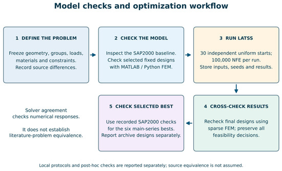
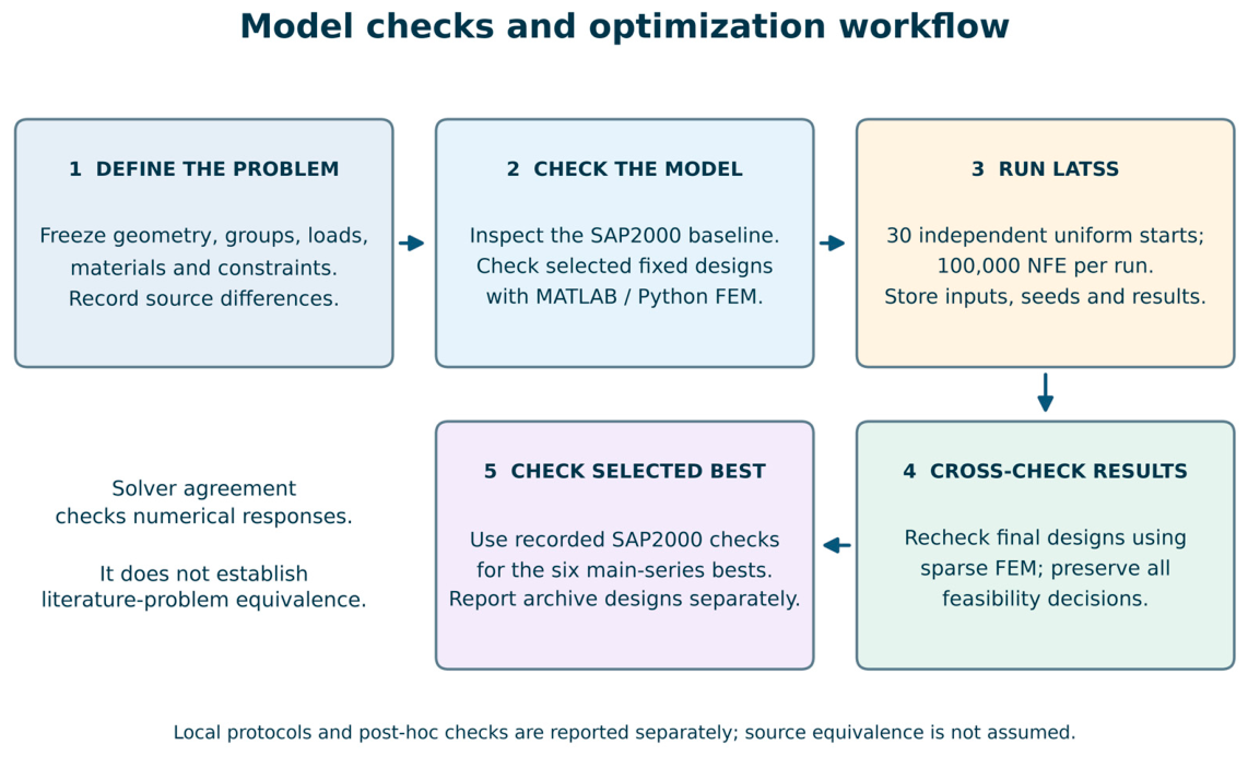
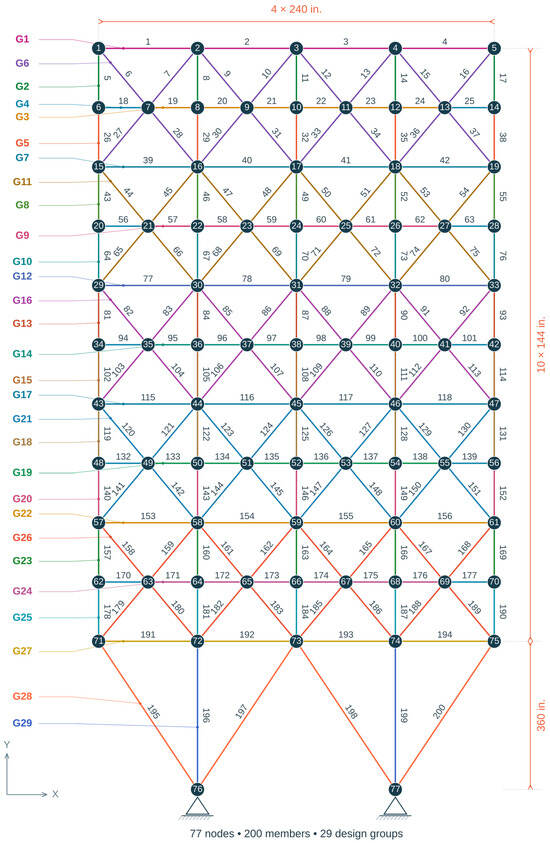
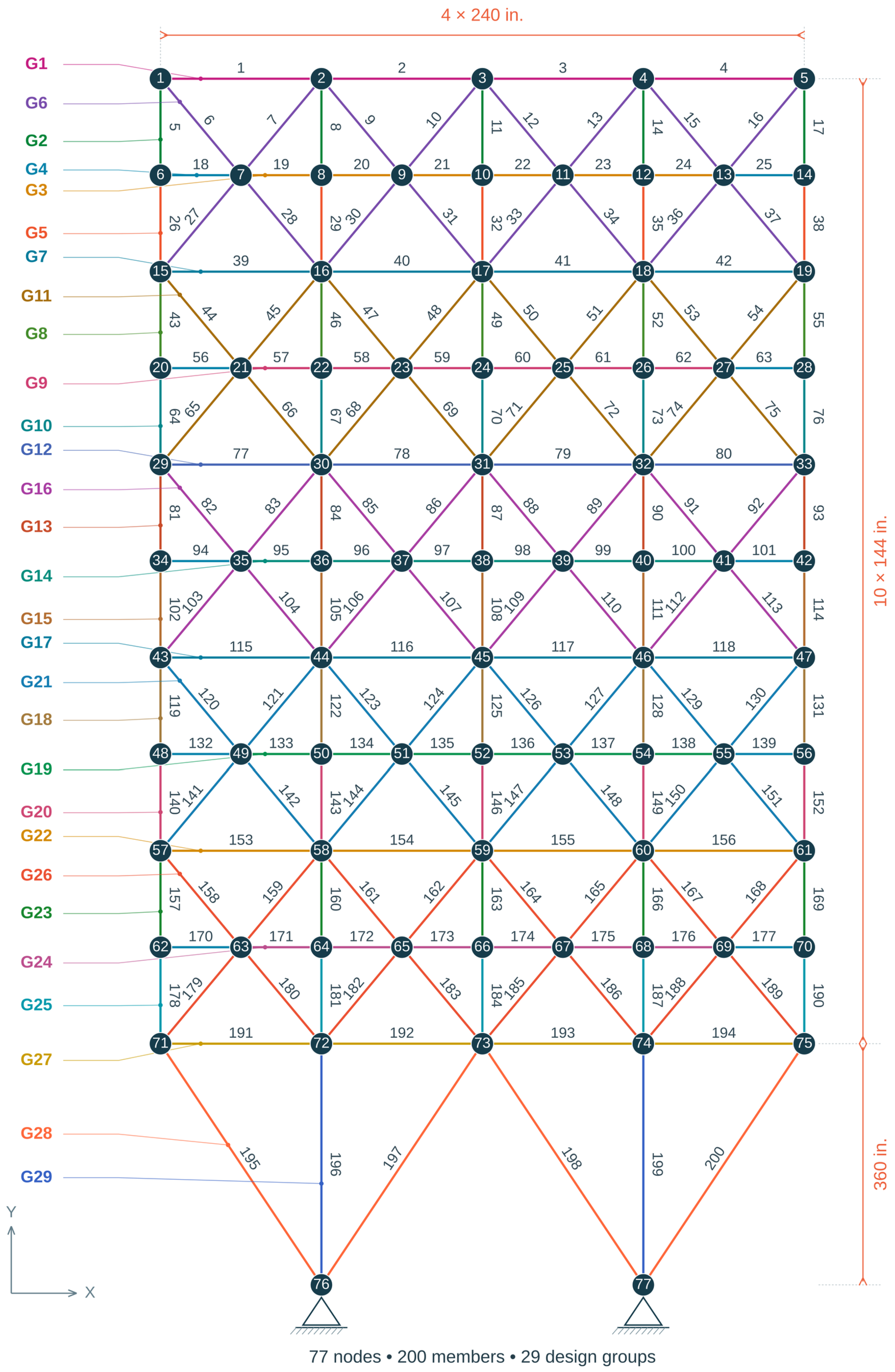
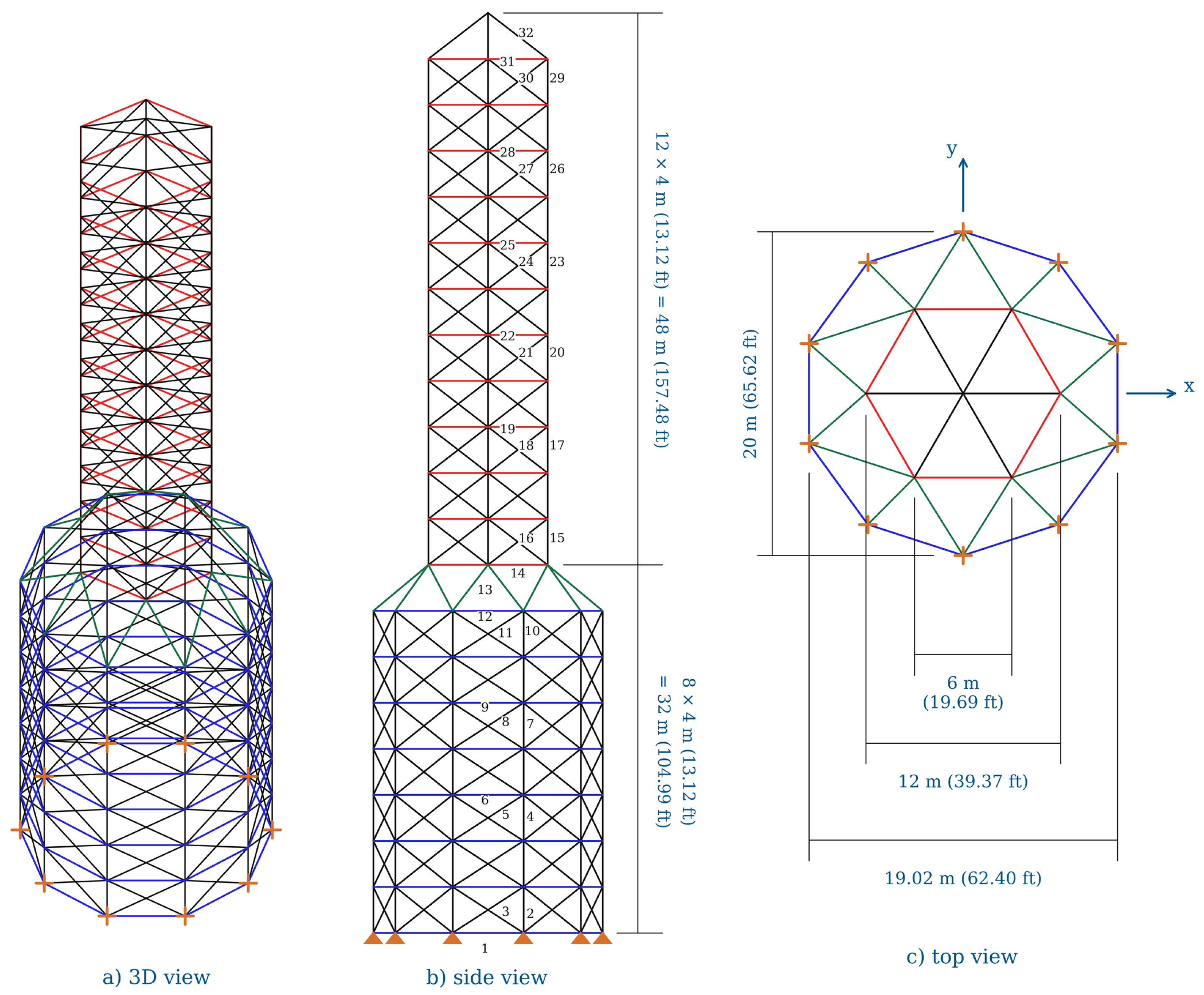
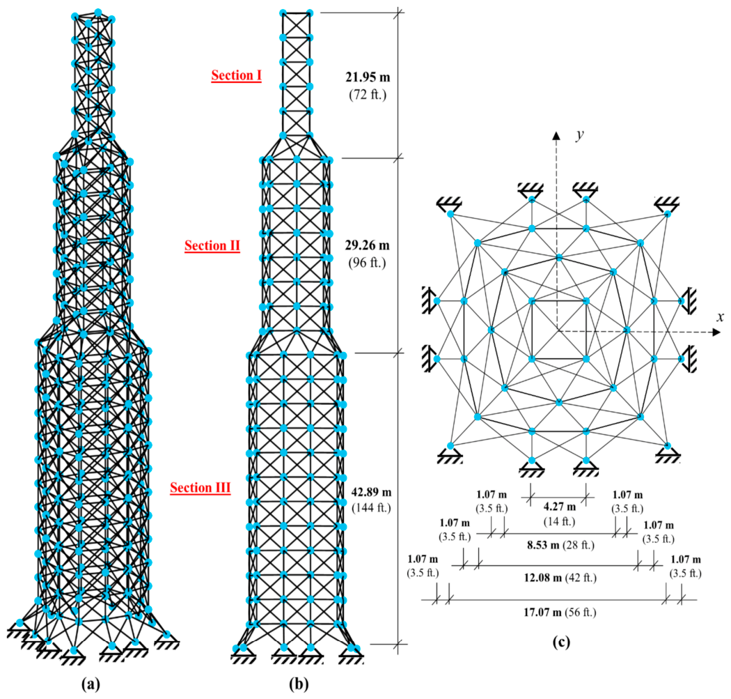
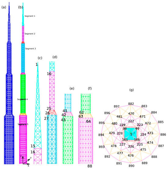
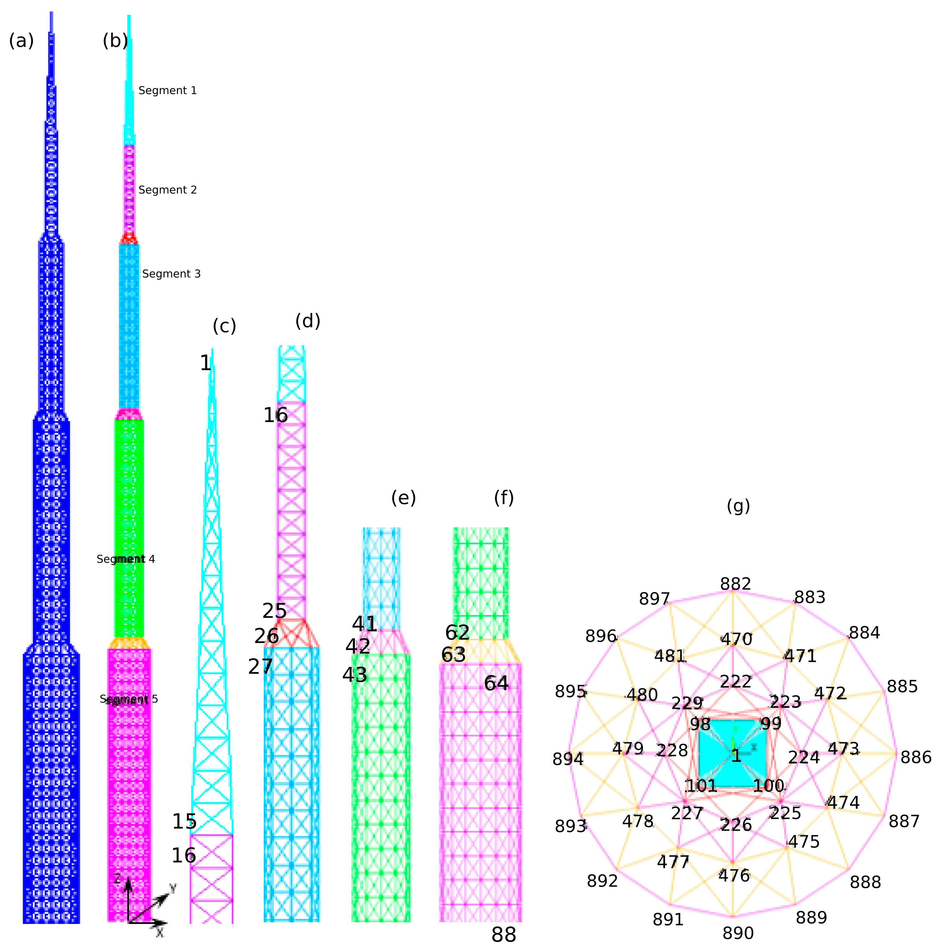
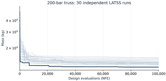
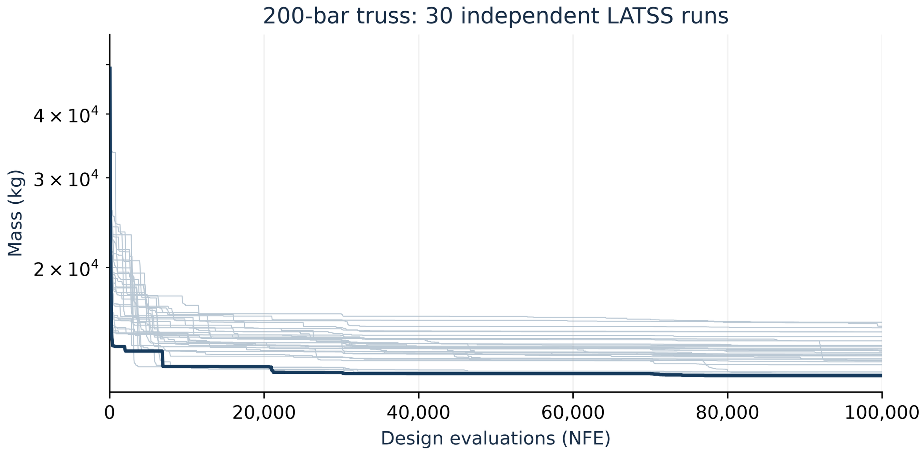
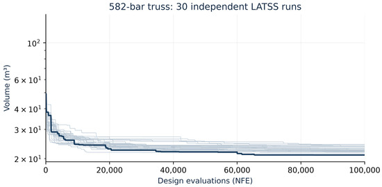
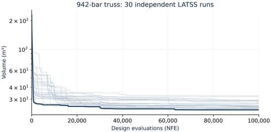
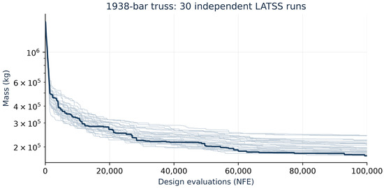
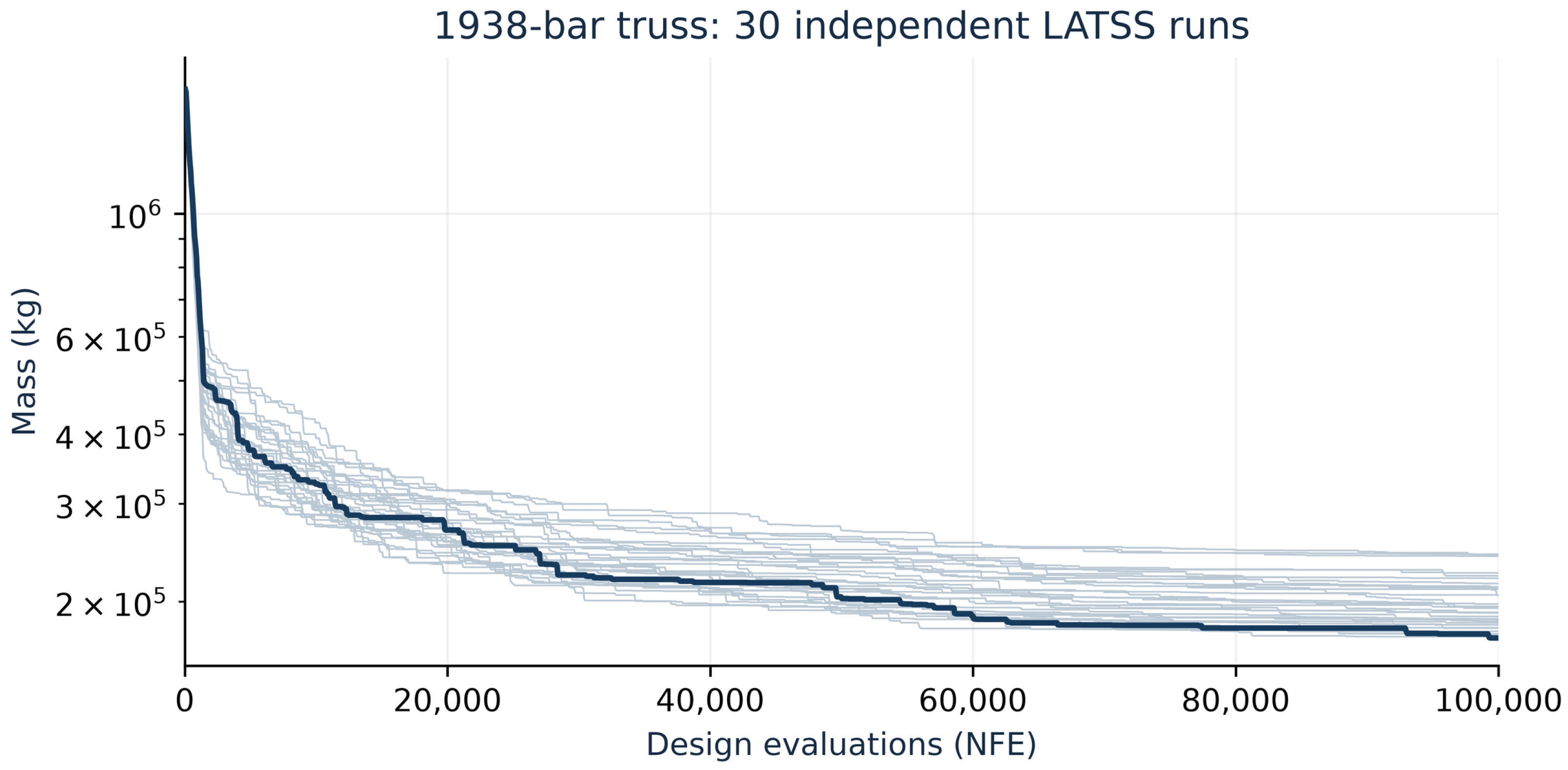
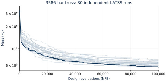
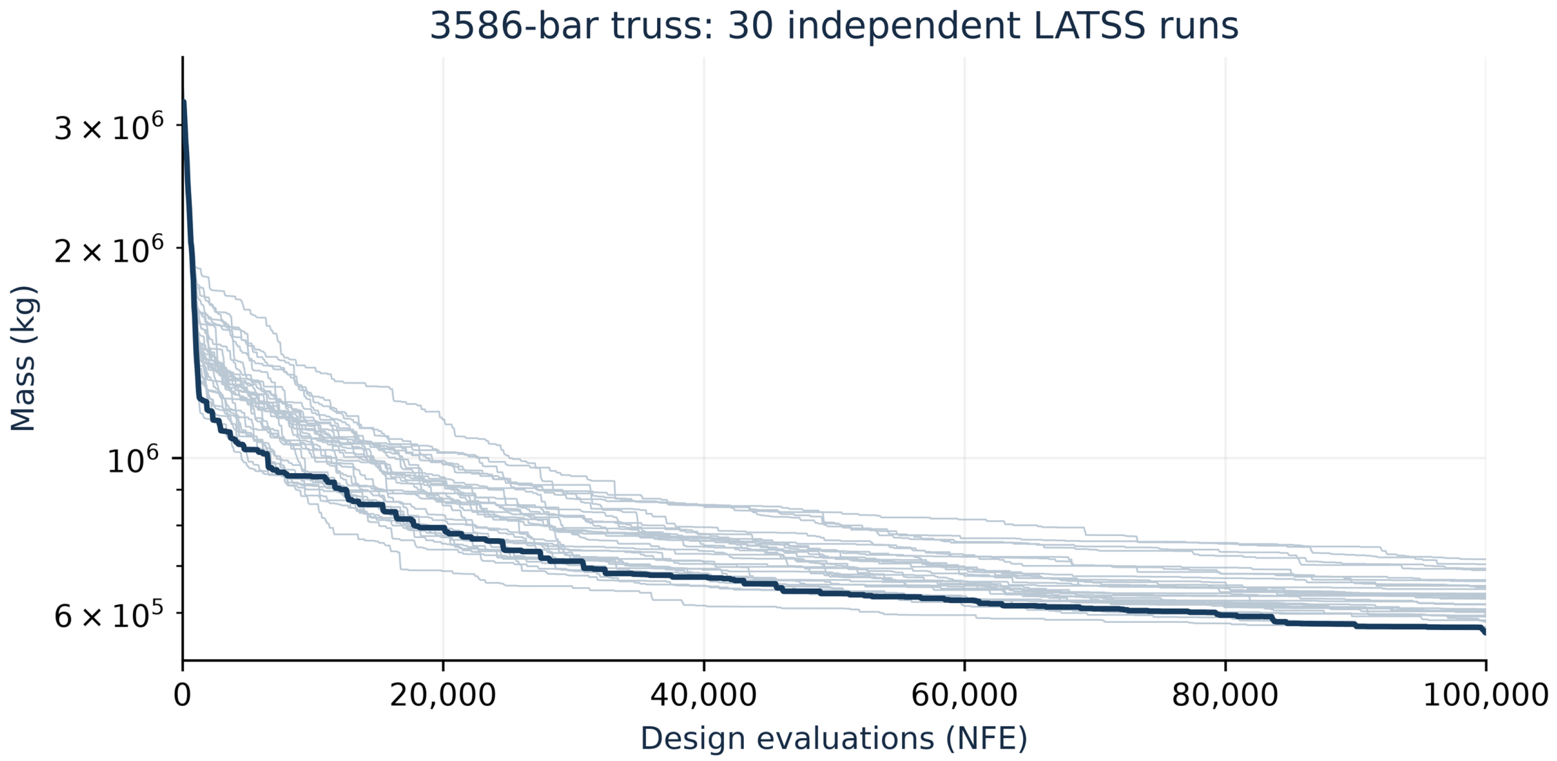
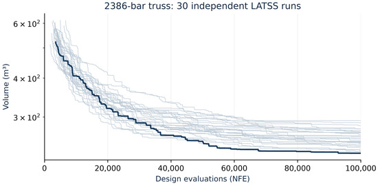
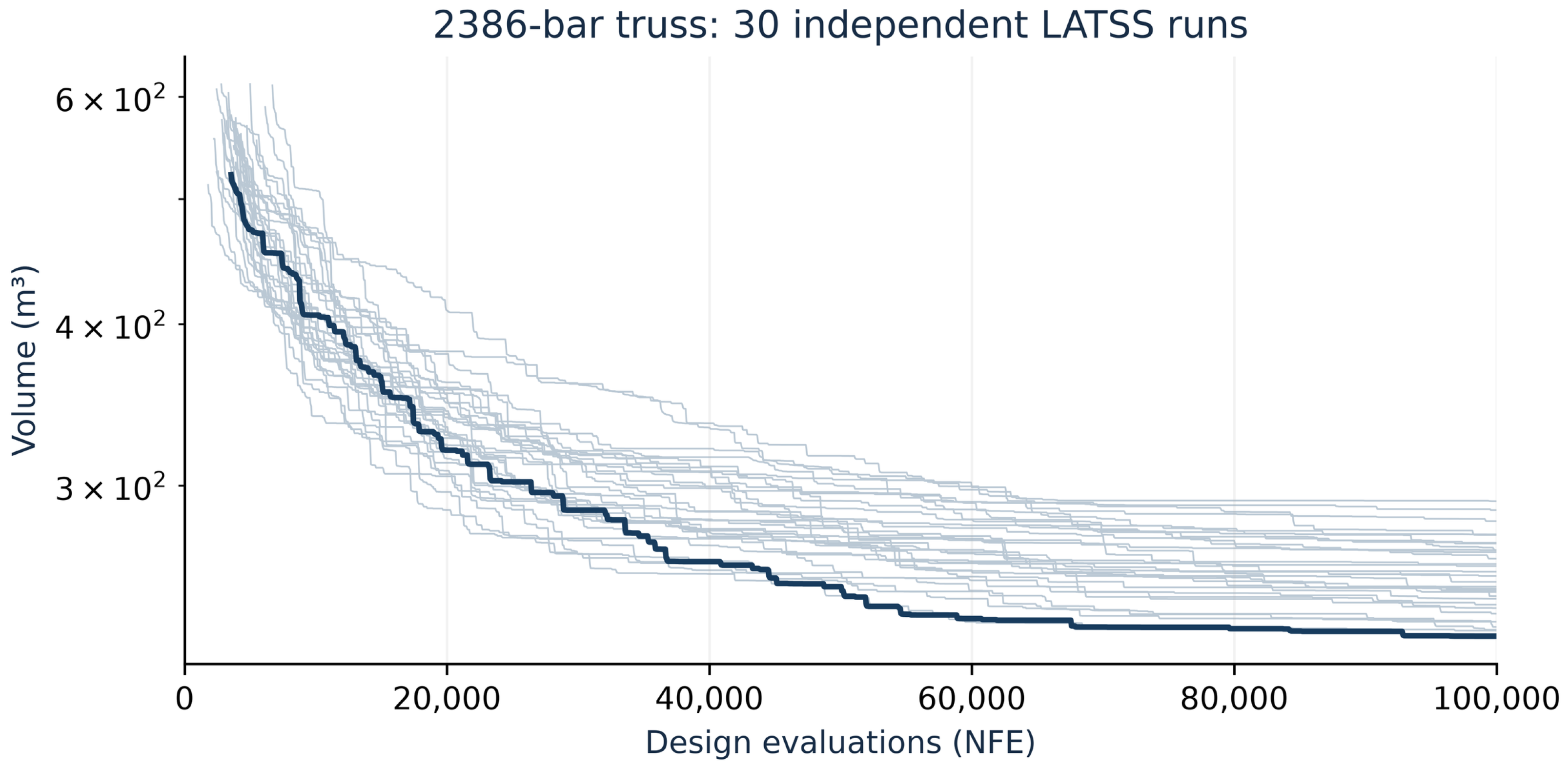
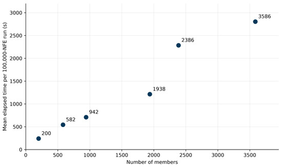
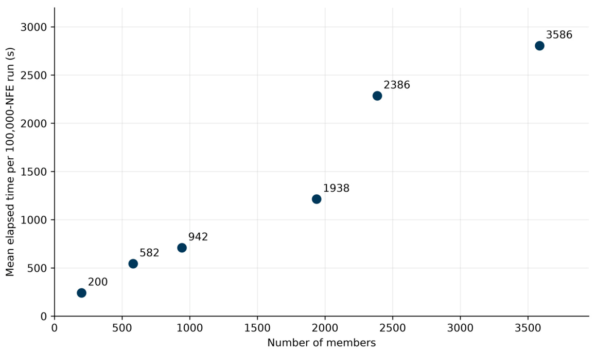

Disclaimer/Publisher’s Note: The statements, opinions and data contained in all publications are solely those of the individual author(s) and contributor(s) and not of MDPI and/or the editor(s). MDPI and/or the editor(s) disclaim responsibility for any injury to people or property resulting from any ideas, methods, instructions or products referred to in the content. |
© 2026 by the author. Licensee MDPI, Basel, Switzerland. This article is an open access article distributed under the terms and conditions of the Creative Commons Attribution (CC BY) license.