Multi-Level Carbon Emission Hotspot Identification and Low-Carbon Optimization of Teaching Buildings Based on BIM Technology

Abstract

Taking a reinforced-concrete frame teaching building at a university as a case study, this study established a carbon emission accounting framework based on BIM-derived quantities, identified carbon emission hotspots at the stage, material, and component levels, and comprehensively evaluated the accounting results and emission reduction potential through sensitivity analysis, Monte Carlo uncertainty analysis, and low-carbon scenario assessment. The results showed that the total A1–A5 carbon emissions of the case-study building were 16,812.69 tCO₂e, corresponding to a carbon emission intensity of 442.51 kgCO₂e/m², of which modules A1–A3 accounted for 94.40%. C35 concrete, reinforcing steel, and autoclaved aerated concrete blocks collectively contributed 88.1% of A1–A3 emissions, while reinforcing steel, infill walls, and floor slabs constituted the major component-level hotspots. Monte Carlo simulation showed that the baseline accounting result fell within the main probability distribution range, while the integrated optimization scenario reduced total A1–A5 carbon emissions by 7.72%. This study quantified carbon emissions from the building material production, transportation, and construction stages (A1–A5) of a teaching building and identified priority targets for emission reduction. The results provide a quantitative basis for low-carbon material selection, key component control, and construction-stage optimization of teaching buildings in China.

1. Introduction

Research on carbon reduction in the building sector is increasingly expanding from operational energy consumption control to whole-life-cycle carbon management. As building operational energy efficiency improves, the relative contribution of embodied carbon arising from building material production, transportation, and construction continues to increase within life-cycle emissions [1,2]. Carbon emissions generated during building material production (A1–A3), transportation (A4), and construction (A5) occur before a building enters operation, meaning that the main opportunities for emission reduction are concentrated in the early design and construction stages and are therefore characterized by strong upfront and lock-in effects.

In reinforced-concrete public buildings, material types, quantities, and structural systems are major factors affecting upfront carbon emissions [3]. Studies of university buildings have also shown that structural systems and material composition can significantly influence building life-cycle carbon emissions [4,5]. Evidence from building case studies in China indicates that concrete, reinforcing steel, and masonry blocks often constitute the principal emission sources during the material production stage [6]. Although the contributions of A4 transportation and A5 construction are generally lower than those of the material production stage, transportation distance, construction energy consumption, and on-site management can still affect upfront emissions [7]. Therefore, accounting only for total building emissions is insufficient to support targeted emission reduction decisions; the specific contributions of individual materials and building components must also be identified.

The development of BIM has provided a structured and digital data foundation for building carbon emission accounting. Previous studies have explored BIM–LCA integration frameworks, data structures, and continuous assessment approaches [8,9], with research gradually extending to early-stage design decision-making, automated component–material–emission factor mapping, and embodied carbon assessment [10,11]. In recent years, openBIM-based automated A1–A5 accounting and component-level life-cycle carbon management frameworks have further improved the efficiency of digital carbon accounting [12]. Recent research has also applied the BIM–LCA workflow to the design of kindergarten buildings, evaluating potential decarbonization strategies at the design stage by comparing the carbon emissions associated with different material options during stages A1–A3 [13]. However, current research still faces challenges related to model data standardization, emission factor matching, and the regional applicability of carbon emission data.

In addition to data mapping issues, building carbon emission accounting is also affected by uncertainties in parameters such as material quantities, carbon emission factors, transportation distances, and construction energy consumption. Previous reviews have shown that parameter values, scenario settings, and model assumptions can all influence building LCA results [14,15]. Monte Carlo simulation combined with sensitivity analysis can extend a single deterministic result into a probability distribution and has been applied to embodied carbon assessments of educational buildings and different structural systems [16,17], providing a methodological basis for quantifying uncertainty and identifying key parameters.

Current low-carbon research is gradually shifting from carbon emission accounting toward hotspot identification and design optimization. Existing studies have shown that structural material combinations, concrete and reinforcing steel parameters, building envelope materials, and early-stage structural design all offer potential for carbon emission reduction [18,19]. However, for actual university teaching buildings, relatively few studies have integrated A1–A5 carbon emission accounting, multi-level hotspot identification across the stage, material, and component levels, parameter uncertainty analysis, and emission reduction scenario assessment within a unified analytical framework.

This study takes a reinforced-concrete frame teaching building as a case study and uses actual component quantities extracted from the BIM model to establish an A1–A5 carbon emission accounting framework covering the building material production and construction stages. Carbon emission hotspots were identified at three levels—life-cycle stage, building material, and BIM component—to determine the major high-contribution materials and their corresponding components. One-factor sensitivity analysis and Monte Carlo uncertainty analysis were then used to identify the key parameters affecting the accounting results and to evaluate the stability of hotspot identification under parameter variation. In addition, low-carbon optimization scenarios involving structural materials, building envelope materials, transportation, and integrated measures were established to compare the potential effects of different emission reduction pathways. The study aims to develop a complete analytical chain comprising “quantity takeoff–carbon emission accounting–hotspot identification–uncertainty analysis–emission reduction optimization,” thereby providing a reusable methodological reference for low-carbon decision-making during the design, material procurement, and construction stages of reinforced-concrete public buildings with similar material systems and construction characteristics.

2. Research Framework and Methods

2.1. Case Studies in Architecture and BIM-Based Quantity Takeoff

The case study focuses on a teaching building with a reinforced-concrete frame structure, primarily used for teaching and associated support functions. The building comprises five above-ground stories and one basement level, with a total floor area of 37,994.20 m² and an overall height of 21.90 m. The above-ground and basement floor areas are 34,997.00 m² and 2997.20 m², respectively. The primary structural system consists mainly of concrete and reinforcing steel, while the building envelope includes autoclaved aerated concrete block walls, aluminum-framed exterior windows, and glass curtain walls.

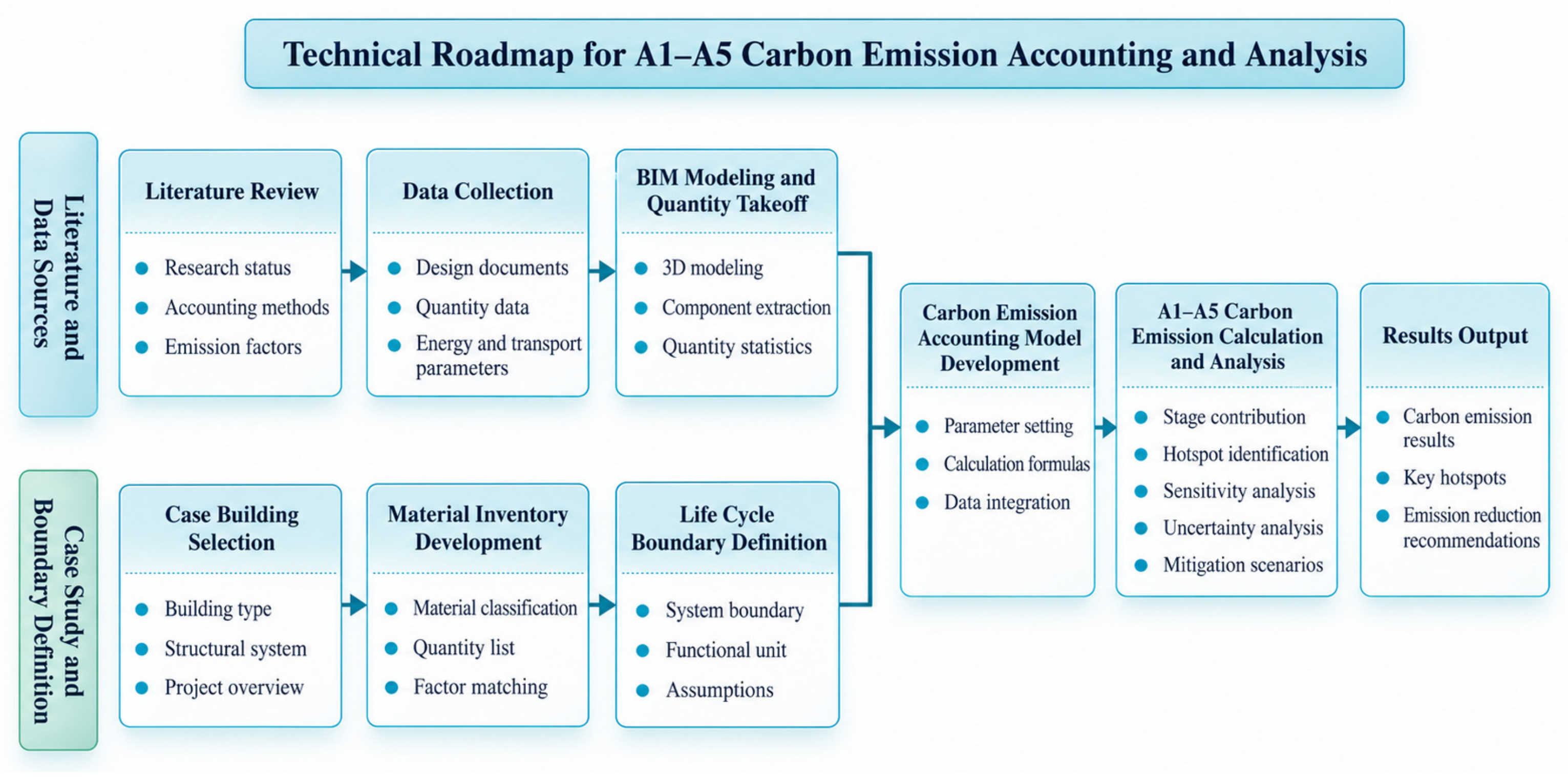
The research workflow is based on BIM-derived quantity takeoff data and sequentially comprises A1–A5 carbon emission accounting, multi-level hotspot identification, sensitivity and uncertainty analyses, and low-carbon scenario evaluation. The overall research framework is illustrated in Figure 1.

Figure 1. BIM-based carbon emission assessment framework for the building construction stage.

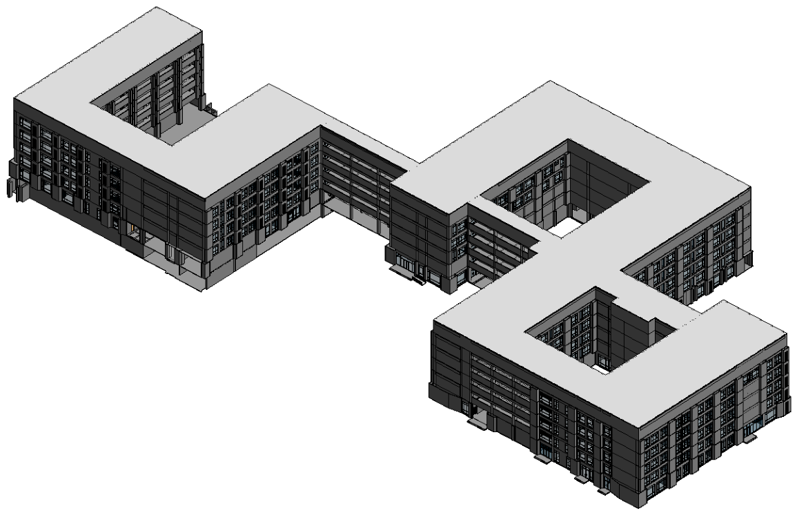
A BIM model of the case-study building was developed using Autodesk Revit 2016, as shown in Figure 2. Quantity takeoff data were extracted from the geometric information and material properties of the building components, and a “component–material–carbon emission factor” mapping relationship was established to provide the basic data for A1–A5 carbon emission accounting [20,21]. Beams, columns, floor slabs, and staircases were uniformly assigned to C35 ready-mixed concrete, while infill walls were mapped to B06 autoclaved aerated concrete blocks; solid exterior walls were quantified separately. Roof construction layers and structural floor slabs were also quantified separately, whereas exterior windows and curtain walls were measured by area.

Figure 2. BIM model of the case-study teaching building.

As the BIM model did not include explicit reinforcement information, the quantity of reinforcing steel was estimated based on the steel content per unit floor area:

$$M_s={\displaystyle \frac{A{q}_s}{1000}}$$

(1)

In the formula, M_s denotes the total mass of reinforcing steel (t), A is the total floor area (m²), and q_s is the reinforcing steel content per unit floor area (kg/m²). In this study, q_s was set to 55 kg/m², yielding an estimated reinforcing steel quantity of 2089.68 t.

To assess the engineering-scale reasonableness of the main structural quantities and the estimated reinforcing steel quantity, the structural concrete consumption and reinforcing steel content per unit floor area were selected as representative indicators and compared with reference ranges for similar teaching buildings [22]. In addition, the A1–A3 carbon emission intensity associated with concrete and reinforcing steel was compared with those reported for existing educational building case studies to verify that the results were of a comparable order of magnitude.

2.2. System Boundary and Carbon Emission Accounting Methods

This study employed the life cycle assessment (LCA) method to quantify carbon emissions from the building material production and construction stages of the case-study building [23,24]. The system boundary was defined as modules A1–A5, where A1 denotes raw material supply, A2 raw material transportation, A3 building material manufacturing, A4 transportation of building materials to the construction site, and A5 construction activities. Modules A1–A3 are collectively referred to as the product stage [25]. The building use, demolition, and recovery and recycling stages were excluded from the assessment. The results are expressed in terms of total carbon emissions (tCO₂e) and carbon emission intensity per unit floor area (kgCO₂e/m²).

2.2.1. Building Materials Production Stage

For modules A1–A3, carbon emissions from building material production were calculated based on the bill of quantities obtained in Section 2.1 by matching the quantities of major building materials with their corresponding carbon emission factors. Carbon emission factors were preferentially obtained from GB/T 51366—2019 and the Guidelines for Carbon Emission Calculation of Civil Buildings in Jiangsu Province [26,27]. For materials without directly corresponding emission factors in these standards, interpolation, unit conversion, or proxy factors were applied according to material properties, units of measurement, and engineering applications. The quantities and carbon emission factors of the main building materials are presented in Table 1. The classification of modules A1–A3 followed the life-cycle stage definitions used in building environmental assessment [28].

Table 1. Quantities and carbon emission factors of major building materials.

Building Material	Quantity	Unit	Carbon Emission Factor	Unit	Methods for Obtaining Emission Factors
C35 ready-mixed concrete	18,270.53	m3	301.50	kgCO2e/m3	Linear interpolation based on the C30 and C50 concrete factors
HRB reinforcing steel (estimated)	2089.68	t	2340.00	kgCO2e/t	Directly reference standard factors
B06 autoclaved aerated concrete blocks	10,959.82	m3	327.00	kgCO2e/m3	Directly reference the corresponding grade factor
Thermally broken aluminum-framed exterior windows (100% primary aluminum)	5660.90	m2	254.00	kgCO2e/m2	Citation Impact Factor
XPS insulation	34.87	t	5020.00	kgCO2e/t	Based on data from the reference database, the quantities were converted using density factors
C20 fine-aggregate concrete	362.27	m3	227.50	kgCO2e/m3	Refer to the standard factors for C20 ready-mix concrete
Glass curtain wall	271.05	m2	254.00	kgCO2e/m2	Factors influencing the selection of thermal break aluminum alloy exterior windows
M15 ready-mixed mortar	181.14	m3	354.75	kgCO2e/m3	Based on the M15 dry-mix floor mortar factors
Concrete wall (solid exterior wall)	203.30	m3	301.50	kgCO2e/m3	Continue to use the C35 concrete interpolation factor

The sources of the carbon emission factors, unit conversion procedures, and proxy factor treatments for each material are provided in Appendix A (Table A2). Materials lacking either production-stage carbon emission factors or independently quantified material quantities were excluded from the A1–A3 baseline calculation, but were not assumed to have zero emissions. This method may lead to an underestimation of actual carbon emissions. Therefore, the total carbon emissions calculated in this study reflect only those associated with the materials included in the available bill of materials.

The total carbon emissions from the building material production stage were calculated as follows:

$$C_{A1-A3}={\displaystyle \sum _{i=1}^n\frac{Q_{i}E{F}_i}{1000}}$$

(2)

In the formula, C_A1–A3 represents the carbon emissions from the building material production stage (tCO₂e), Q_i denotes the quantity of the i-th material, EF_i is the corresponding carbon emission factor, and n is the number of material types. All units were standardized during the calculation, and 1000 was used as the unit conversion factor.

2.2.2. Building Material Transportation Stage

Carbon emissions in module A4 arise from the transportation of building materials from supply locations to the construction site. These emissions are primarily affected by the transported mass, transportation distance, and transport mode [29]. As complete transportation records were unavailable, typical supply distances and the corresponding vehicle-specific emission factors were adopted for estimation.

Carbon emissions from the building material transportation stage were calculated as follows:

$$C_{A4}={\displaystyle \sum _{i=1}^n\frac{M_i{D}_i{T}_i}{1000}}$$

(3)

In the formula, C_A4 represents the carbon emissions from the transportation stage (tCO₂e), M_i denotes the transported mass of the i-th material (t), D_i is the average transportation distance (km), and T_i is the transportation emission factor [kgCO₂e/(t·km)].

2.2.3. Construction Stage

Module A5 primarily accounts for electricity and diesel consumption during construction [30]. Due to the lack of on-site measured energy consumption data, construction energy consumption intensities per unit floor area were used for estimation. The relevant parameters and their uncertainty ranges are provided in Appendix A.

Carbon emissions from the construction stage were calculated as follows:

$$C_{A5}={\displaystyle \frac{A(E_{e}E{F}_e+E_{d}E{F}_d)}{1000}}$$

(4)

In the formula, C_A5 represents the carbon emissions from the construction stage (tCO₂e), A denotes the total floor area of the building (m²), E_e and E_d represent the construction electricity consumption intensity (kWh/m²) and diesel consumption intensity (L/m²) per unit floor area, respectively, and EF_e and EF_d are the corresponding carbon emission factors for electricity and diesel, respectively.

2.2.4. Carbon Emission Summary

After the calculations for modules A1–A3, A4, and A5 were completed, the emissions from each stage were summed to obtain the total carbon emissions from building material production and construction:

C_total = C_A1−A3 + C_A4 + C_A5

(5)

The carbon emission intensity per unit floor area was calculated as follows:

$$I_C={\displaystyle \frac{1000C_{\mathit{total}}}{A}}$$

(6)

In the formula, C_total represents the total carbon emissions from modules A1–A5 (tCO₂e), I_C denotes the carbon emission intensity per unit floor area (kgCO₂e/m²), and A is the total floor area of the building (m²). In this study, the total floor area of 37,994.20 m² specified in the design documents was used as the denominator for the intensity calculation.

2.3. Multi-Level Carbon Emission Hotspot Identification Method

To identify the primary carbon emission sources across modules A1–A5 of the case-study building, hotspot analysis was conducted at three levels: life-cycle stage, building material, and BIM component. At the stage level, the relative contributions of modules A1–A3, A4, and A5 were compared. At the material level, high-contribution building materials were identified. At the component level, the A1–A3 emission contributions associated with different building components were quantified based on BIM-derived quantity takeoff data. The carbon emission contribution of each analytical object was calculated as follows:

$$P_j={\displaystyle \frac{C_j}{C_{\mathit{ref}}}}\times 100\%$$

(7)

In the formula, P_j represents the carbon emission contribution rate (%) of the j-th category, C_j denotes the carbon emissions (tCO₂e) associated with the corresponding stage, material, or component, and C_ref is the reference total carbon emissions for the corresponding analytical level. At the stage level, total A1–A5 emissions were used as the denominator, whereas at the material and component levels, A1–A3 building material production emissions were used as the denominator. To evaluate the concentration of carbon emissions, the analyzed objects were ranked in descending order of carbon emissions, and the cumulative contribution rate was calculated as follows:

$$K_m={\displaystyle \sum _{j=1}^m{P}_j}$$

(8)

In the formula, K_m represents the cumulative contribution rate (%) of the top m categories and is used to characterize the degree to which carbon emissions are concentrated among a limited number of materials or components.

2.4. Sensitivity Analysis Method

Based on the hotspot identification results and the specified parameter ranges, a one-at-a-time sensitivity analysis was conducted for key parameters, including reinforcing steel content, carbon emission factors of major building materials, transportation distances, and construction energy consumption intensities [17]. During the analysis, all other parameters were held constant while only the target parameter was varied, and the resulting changes in total A1–A5 carbon emissions relative to the baseline scenario were evaluated. For glass curtain walls, for which a proxy emission factor was adopted, a further one-at-a-time sensitivity analysis was conducted. While keeping the baseline values of all other parameters constant, the emission factor for glass curtain walls was varied individually within the range of 194–254 kgCO₂e/m² to evaluate its impact on total carbon emissions.

The change in carbon emissions induced by parameter variation was calculated as follows:

ΔC_k = C_k − C₀

(9)

In the formula, ΔC_k represents the change in carbon emissions caused by variation in the k-th parameter (tCO₂e), C_k denotes the total carbon emissions after adjustment of the parameter, and C₀ is the total A1–A5 carbon emissions under the baseline scenario.

The relative change rate was calculated as follows:

$${\eta }_k={\displaystyle \frac{C_k-C_0}{C_0}}\times 100\%$$

(10)

In the formula, η_k represents the relative change rate (%) corresponding to variation in the k-th parameter. The parameter ranges were determined based on standard values, engineering experience, and the ranges observed in the available data.

2.5. Monte Carlo-Based Uncertainty Analysis Method

One-factor sensitivity analysis primarily captures the effect of variation in an individual parameter and cannot adequately characterize changes in the results when multiple parameters vary simultaneously [20]. Therefore, Monte Carlo simulation was employed for uncertainty analysis. The key parameters were treated as random variables, assumed to be mutually independent, and assigned triangular probability distributions. A total of 5000 random samples were generated. In the Monte Carlo simulation, the input variables used for building carbon emission accounting, including material emission factors, engineering quantities, transportation distances, and construction energy consumption, were obtained from different sources. Given the lack of sufficient data to establish correlations among these variables, all input parameters were assumed to be mutually independent. However, this independence assumption represents a simplification under data-limited conditions. If correlations exist among the parameters in practice, they may affect the probability distribution and uncertainty intervals of the simulation results. Regarding the selection of probability distributions, the limited availability of statistical data for some input parameters makes it difficult to establish precise probability distribution models. Therefore, triangular distributions were adopted to characterize parameter uncertainty. The triangular distribution accounts for the minimum, most likely, and maximum values of each parameter, making it suitable for uncertainty analysis in engineering assessments where data availability is limited. The lower bound, mode, upper bound, and random seed used for each parameter are provided in Appendix A. To assess the stability of the ranking of major emission sources in the Monte Carlo simulations, the carbon emissions of the major materials were ranked in each simulation run. The “ranking stability rate” was defined as the proportion of the total simulation runs in which the original ranking of emission sources was maintained.

To verify the adequacy of the number of Monte Carlo simulations, a convergence analysis was further conducted in this study. The stability of the simulation results was evaluated by comparing the mean carbon emissions for stages A1–A5 obtained from different numbers of simulation runs (500, 1000, 2000, 3000, 4000, and 5000). The results indicate that the mean carbon emissions gradually converged as the number of simulations increased. When the number of simulation runs reached 5000, the mean carbon emissions were 16,747.96 tCO₂e, showing only minor variations compared with the results obtained from fewer simulation runs. These findings indicate that 5000 simulation runs were sufficient to ensure the stability of the uncertainty analysis results in this study (see Figure S1 in the Supplementary Materials for the convergence analysis results).

The carbon emission result for the r-th random sample can be expressed as follows:

$$C^{(r)}=f(X_1^{(r)},X_2^{(r)},\dots ,X_p^{(r)})$$

(11)

In the formula, C^(r) represents the total A1–A5 carbon emissions obtained from the r-th sample, and $X_p^{\left(r\right)}$ denotes the value of the p-th uncertain parameter in the r-th sample. The probability distribution of total carbon emissions was obtained through repeated sampling, and its distribution characteristics were described using the mean, median, standard deviation, and the 5th–95th percentile range.

2.6. Low-Carbon Optimization Scenario Design

Based on the hotspot identification and sensitivity analysis results, low-carbon optimization scenarios were established to compare the potential effects of different emission reduction pathways. The term “low-carbon optimization” in this study primarily refers to carbon emission reduction. Based on the identification of major emission hotspots and sensitive parameters, it involves scenario-based adjustments to key materials and related parameters to compare the potential emission reduction effects of different scenarios. It does not represent a comprehensive engineering optimization that simultaneously accounts for multiple constraints, such as cost, structural performance, and material availability. The scenario design focused on structural materials, building envelope materials, transportation distances, and integrated optimization [30]. Six scenarios were considered: a baseline scenario, structural concrete optimization, low-carbon reinforcing steel, building envelope material optimization, transportation optimization, and integrated optimization. In particular, the comprehensive optimization scenario S5 was calculated by aggregating the emission reductions achieved in the four individual scenarios (S1–S4), without explicitly accounting for potential interactions among the different optimization measures.

The emission reduction rate for each scenario was calculated as follows:

$$R_S={\displaystyle \frac{C_0-C_S}{C_0}}\times 100\%$$

(12)

In the formula, R_s represents the emission reduction rate (%) for the s-th scenario, C_s denotes the total A1–A5 carbon emissions under that scenario (tCO₂e), and C₀ is the total carbon emissions under the baseline scenario. The scenario analysis was primarily conducted to quantify the potential emission reduction effects of different low-carbon pathways. The practical feasibility of each scenario should be further evaluated by considering structural safety, material availability, and cost constraints.

3. Results

3.1. Baseline Carbon Emission Results and Multi-Level Hotspot Identification

Prior to the baseline carbon emission analysis, an engineering-scale plausibility check was conducted on the main structural quantities and their corresponding emission levels, as presented in Table 2. The structural concrete consumption, reinforcing steel content, and A1–A3 carbon emission intensity of the structural system were all within ranges comparable to those reported in relevant guidelines and previous educational building case studies, indicating that the principal quantity estimates and accounting results were reasonable at the engineering scale. This comparison was intended solely as an order-of-magnitude check and should not be regarded as an independent validation of the accuracy of the BIM-derived quantities.

Table 2. Engineering-scale plausibility check of major quantity indicators and structural-system carbon emission intensity.

Comparison Indicator	This Case	Reference Value	Basis	Description
Structural concrete consumption	0.481 m3/m2	0.45–0.50 m3/m2	Guidelines for Carbon Emission Calculation of Civil Buildings in Jiangsu Province [27]	Within the reference range
Reinforcing steel content per unit floor area	55 kg/m2	50–60 kg/m2	Guidelines for Carbon Emission Calculation of Civil Buildings in Jiangsu Province [27]	Within the reference range
A1–A3 carbon emission intensity of concrete and reinforcing steel	273.7 kgCO2e/m2	261.3 kgCO2e/m2	Teaching building case in Zhongshan [31]	Comparable order of magnitude
A1–A3 carbon emission intensity of concrete and reinforcing steel	273.7 kgCO2e/m2	304 kgCO2e/m2	Structural-system results for an educational building reported by Gillott et al. [32]	Comparable order of magnitude

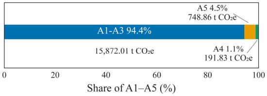
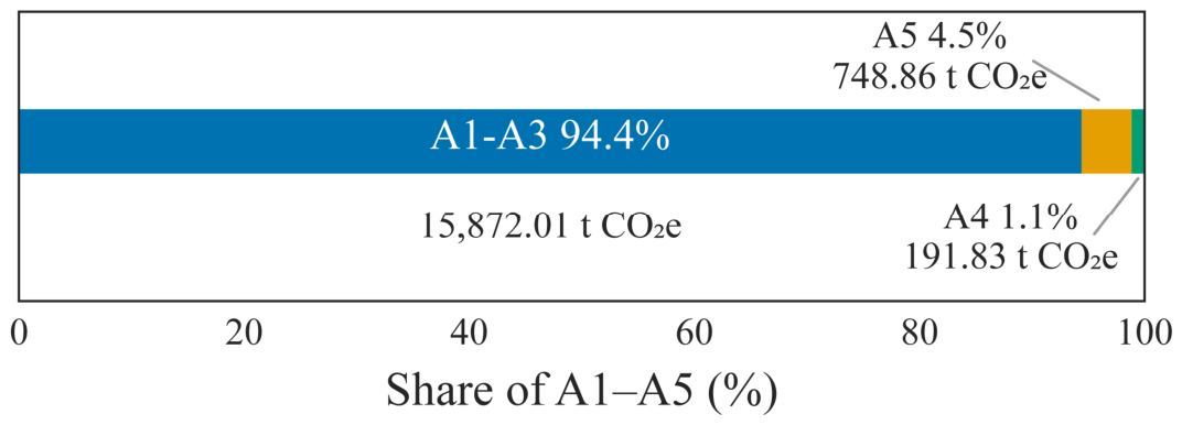
According to the accounting method described in Section 2.2, the total A1–A5 carbon emissions of the case-study building were 16,812.69 tCO₂e, corresponding to a carbon emission intensity of 442.51 kgCO₂e/m². Among these, the A1–A3 building material production stage accounted for 15,872.01 tCO₂e, or 94.40% of the total emissions; the A4 off-site transportation stage contributed 191.83 tCO₂e, or 1.14%; and the A5 construction stage contributed 748.86 tCO₂e, or 4.45%. The detailed accounting results are presented in Table 3, and the carbon emission composition by stage is illustrated in Figure 3.

Table 3. A1–A5 carbon emission accounting results.

Stage	Carbon Emissions (tCO2e)	Carbon Emission Intensity (kgCO2e/m2)	Proportion (%)	Data Description
A1–A3 Building material production	15,872.01	417.75	94.40	Calculated based on BIM-derived quantities and building material carbon emission factors
A4 Off-site transportation	191.83	5.05	1.14	Estimated based on typical supply distances
A5 Construction	748.86	19.71	4.45	Estimated based on construction energy consumption intensity
Total	16,812.69	442.51	100.00	Excluding the use, demolition, and recovery and recycling stages

Figure 3. Composition of A1–A5 carbon emissions.

From the stage-level distribution, carbon emissions from the case-study building were predominantly concentrated in the building material production stage, with modules A1–A3 accounting for more than 90% of the total emissions. Under the parameter settings adopted in this study, emissions from the A5 construction stage were higher than those from the A4 off-site transportation stage. Although A4 involved the transportation of large quantities of materials, its contribution to total emissions remained relatively low under the assumed typical supply distances. Given that the transportation distances for stage A4 and the construction energy parameters for stage A5 are based on estimated values, sensitivity analysis and Monte Carlo simulation were conducted to further evaluate the effects of parameter variations on the calculation results.

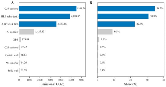
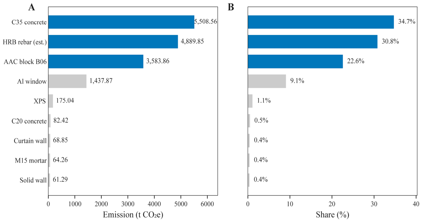
The material-level analysis focused on modules A1–A3, and the carbon emissions associated with the major building materials are shown in Figure 4. C35 ready-mixed concrete contributed 5508.56 tCO₂e, accounting for 34.7% of A1–A3 emissions; HRB reinforcing steel contributed 4889.85 tCO₂e, accounting for 30.8%; and autoclaved aerated concrete blocks contributed 3583.86 tCO₂e, accounting for 22.6%. Aluminum-framed exterior windows accounted for 9.1%, whereas the individual contributions of the remaining materials, including roof insulation, fine-aggregate concrete, curtain walls, mortar, and solid exterior walls, were relatively low.

Figure 4. Carbon emissions of major materials in A1–A3: (A) carbon emissions of individual building materials (tCO₂e); (B) percentage contributions of individual building materials to total A1–A3 emissions (%). Blue bars represent the three materials with the highest carbon emission contributions, while grey bars represent the remaining materials.

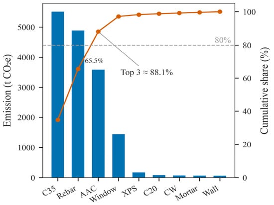
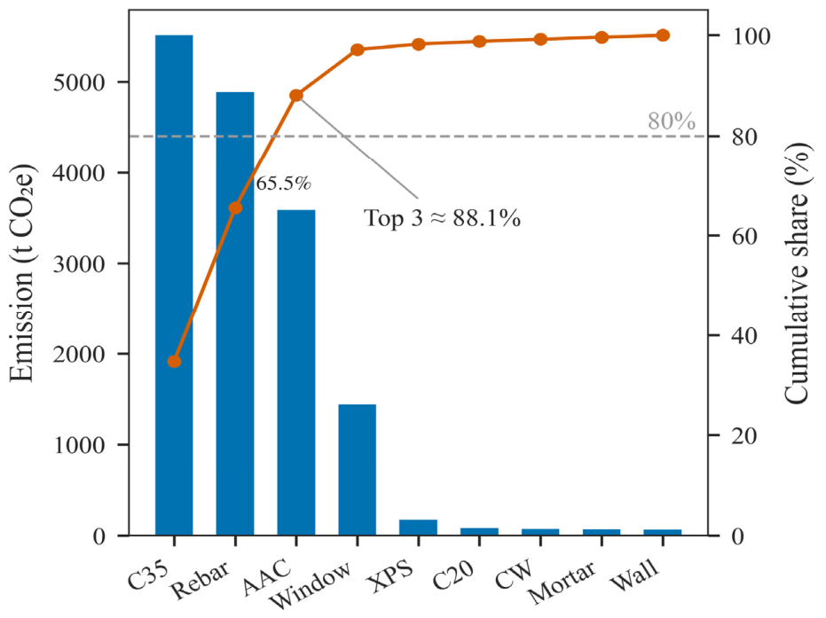
The cumulative contributions of the major materials are shown in Figure 5. C35 concrete and HRB reinforcing steel together accounted for approximately 65.5% of A1–A3 emissions. When autoclaved aerated concrete blocks were included, the cumulative contribution of the top three materials increased to approximately 88.1%. These results indicate that A1–A3 carbon emissions were highly concentrated in a limited number of high-contribution materials, with structural materials and masonry envelope materials constituting the principal material-level hotspots.

Figure 5. Cumulative contribution of major materials to A1–A3 carbon emissions.

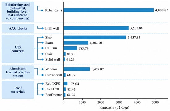
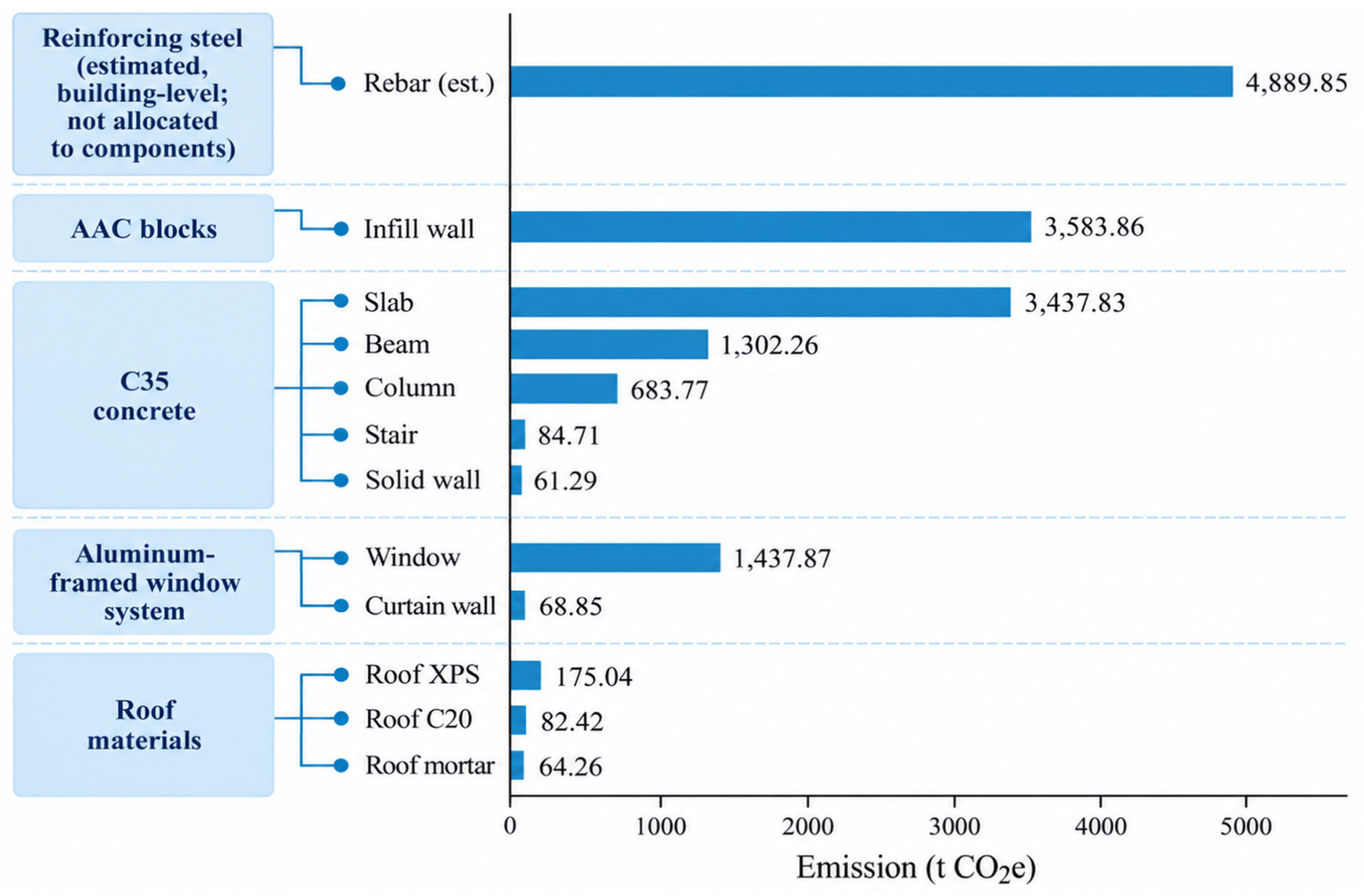
Based on the BIM-derived component quantities, the component-level carbon emission characteristics were analyzed, as shown in Figure 6. Reinforcing steel was reported as a separate item for the entire building, with emissions of 4889.85 tCO₂e, accounting for 30.81% of A1–A3 emissions. Among the materials that could be directly mapped to BIM components, infill walls and floor slabs made relatively large contributions. Infill walls accounted for 3583.86 tCO₂e, or 22.58%, while floor slabs contributed 3437.83 tCO₂e, or 21.66%. Exterior windows accounted for 9.06%, whereas beams and columns contributed 8.20% and 4.31%, respectively. The contributions of the remaining components were comparatively low.

Figure 6. Hierarchical relationships between materials and components and their corresponding carbon emissions.

Because reinforcing steel was not explicitly modeled as BIM entities, its quantity was estimated based on the overall steel content of the building and reported as a separate item rather than being allocated to specific components such as beams, columns, and floor slabs. As shown in Figure 6, excluding this separate item, infill walls and floor slabs were identified as the predominant component-level carbon emission hotspots.

All three levels exhibited a pronounced concentration of carbon emissions. At the stage level, emissions were concentrated in modules A1–A3; at the material level, they were dominated by C35 concrete, reinforcing steel, and autoclaved aerated concrete blocks; and at the component level, the main hotspots were reinforcing steel, infill walls, and floor slabs. These hotspot identification results provided a clear basis for prioritizing the parameters and objects considered in the subsequent sensitivity analysis and low-carbon scenario design.

3.2. Sensitivity Analysis Results

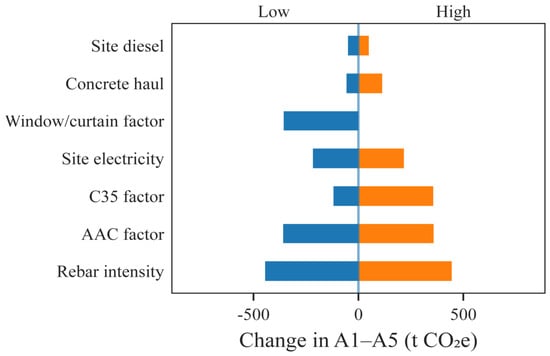
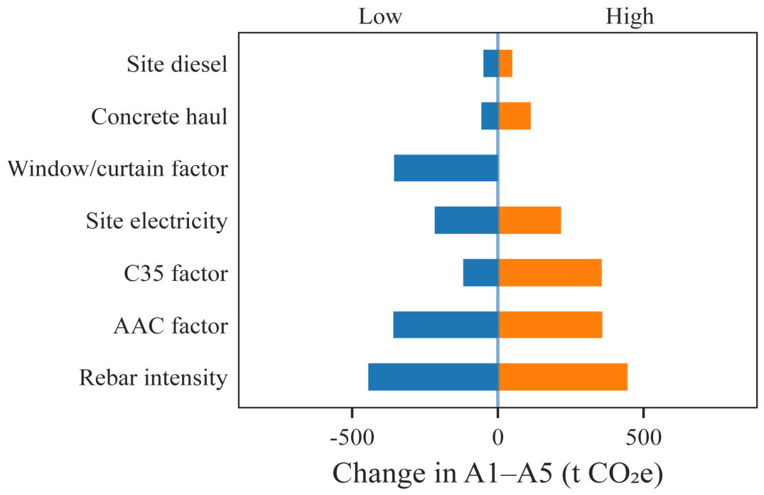
To quantify the effects of key parameter variations on total A1–A5 carbon emissions, a one-factor sensitivity analysis was conducted under the baseline scenario, as shown in Figure 7. The impacts of different parameters on total emissions varied considerably. Reinforcing steel content and the carbon emission factor of autoclaved aerated concrete blocks showed the highest sensitivities, followed by the carbon emission factor of C35 concrete, construction electricity consumption intensity, and the carbon emission factors of exterior windows and curtain walls.

Figure 7. Sensitivity analysis of key parameters on total A1–A5 carbon emissions.

Variations in reinforcing steel content produced the largest fluctuation in total carbon emissions, with a range of approximately 889.06 tCO₂e, followed by the carbon emission factor of autoclaved aerated concrete blocks, with a corresponding range of approximately 716.77 tCO₂e. The carbon emission factor of C35 concrete resulted in a variation of approximately 475.03 tCO₂e, while construction electricity consumption intensity caused a variation of approximately 433.36 tCO₂e. These results indicate that material-related parameters were the dominant factors affecting the baseline carbon accounting results, while construction electricity consumption intensity also exhibited relatively high sensitivity.

The variation in the carbon emission factors of exterior windows and curtain walls resulted in a fluctuation of approximately 355.92 tCO₂e. By contrast, the effects of concrete transportation distance and diesel consumption intensity were relatively small, corresponding to approximately 169.70 tCO₂e and 98.81 tCO₂e, respectively. Within the parameter ranges considered in this study, total A1–A5 carbon emissions were more sensitive to high-volume materials and their associated emission factors, whereas the effects of transportation distance and diesel consumption were comparatively limited. In addition, a separate sensitivity analysis was conducted for the glass curtain wall, for which a proxy emission factor was adopted. The results show that when the curtain wall emission factor varies within the range of 194–254 kgCO₂e/m², total A1–A5 carbon emissions vary by 16.26 tCO₂e, accounting for 0.10% of the baseline total emissions. This indicates that, within the specified parameter range, the proxy emission factor for the glass curtain wall has a relatively minor impact on total carbon emissions. Nevertheless, potential deviations arising from differences between the proxy factor and the actual emission factor of the material cannot be completely ruled out.

The sensitivity ranking was generally consistent with the hotspot identification results. Reinforcing steel, concrete, and autoclaved aerated concrete blocks were not only the major emission sources but also key parameters affecting the stability of the accounting results. Therefore, subsequent low-carbon scenario analysis should prioritize the optimization of structural and envelope materials, while construction electricity consumption should be treated as an important control parameter during the construction stage.

It should be noted that the reinforcing steel content of 55 kg/m² was adopted as an estimated parameter and is therefore subject to a certain degree of uncertainty. Its potential impact on the carbon emission accounting results was quantified through sensitivity analysis. The results indicate that, within the uncertainty range specified in this study, variations in reinforcing steel content primarily affect the absolute value of total A1–A5 carbon emissions but do not substantially alter the contribution patterns of the major emitting materials or the hotspot identification results. Therefore, this parameter assumption does not affect the main conclusions of this study regarding the major emission sources and emission reduction priorities.

3.3. Monte Carlo Uncertainty Analysis Results

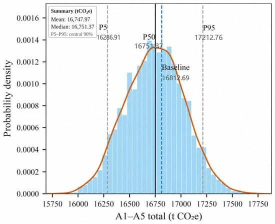
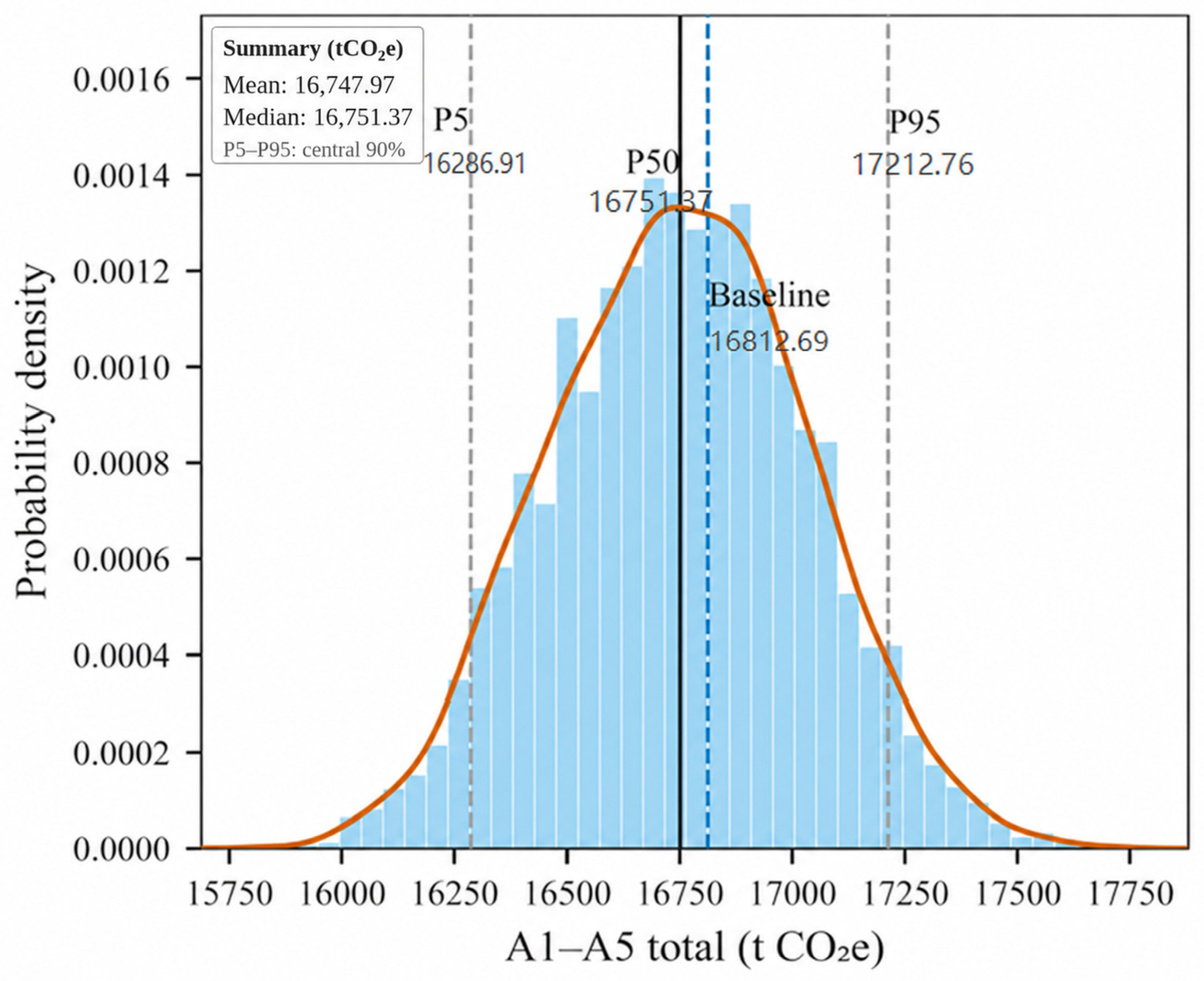
To evaluate the effects of simultaneous variations in multiple parameters on total A1–A5 carbon emissions, 5000 Monte Carlo simulations were performed, as shown in Figure 8. The mean total carbon emissions were 16,747.97 tCO₂e, with a median of 16,751.37 tCO₂e and a standard deviation of 283.32 tCO₂e. The P5 and P95 values were 16,286.91 tCO₂e and 17,212.76 tCO₂e, respectively, corresponding to carbon emission intensities of 428.7–453.0 kgCO₂e/m².

Figure 8. Distribution of total A1–A5 carbon emissions under Monte Carlo simulation.

The results of the 5000 simulations were primarily concentrated around the baseline value, and the baseline accounting result of 16,812.69 tCO₂e fell within the P5–P95 range. The mean value obtained from the Monte Carlo simulation was slightly lower than the baseline accounting result, mainly because a triangular distribution of 194–254 kgCO₂e/m² was assigned to the carbon emission factors of exterior windows and curtain walls in the simulation, whereas the baseline calculation adopted a value of 254 kgCO₂e/m². The combined variations in the other random parameters partially offset or reinforced this difference.

The combined variation in multiple parameters introduced some dispersion in total carbon emissions, although the overall distribution remained relatively concentrated. The carbon emissions of the major materials were ranked in each of the 5000 Monte Carlo simulation runs. The results showed that the relative rankings of C35 concrete, reinforcing steel, and autoclaved aerated concrete blocks remained unchanged throughout all simulation runs, with a ranking stability rate of 100% for each material. Within the specified parameter ranges, the baseline accounting result fell within the main probability distribution range. Reinforcing steel content, the carbon emission factors of major materials, and construction electricity consumption intensity remained the primary sources of uncertainty in total carbon emissions.

3.4. Low-Carbon Optimization Scenario Results

Based on the hotspot identification and sensitivity analysis results, optimization scenarios were established for structural concrete, reinforcing steel, building envelope materials, and transportation, together with an integrated optimization scenario. The carbon emission results for each scenario are presented in Table 4.

Table 4. Carbon emission results under different low-carbon optimization scenarios.

Scenario	Optimization Measure	Total Carbon Emissions (tCO2e)	Carbon Emission Intensity (kgCO2e/m2)	Emission Reduction (tCO2e)	Emission Reduction Rate (%)
S0	Baseline scenario	16,812.69	442.5	0.00	0.00
S1	Structural concrete optimization	16,693.93	439.4	118.76	0.71
S2	Low-carbon reinforcing steel	16,081.30	423.3	731.39	4.35
S3	Building envelope material optimization	16,456.77	433.1	355.92	2.12
S4	Transportation optimization	16,720.77	440.1	91.92	0.55
S5	Integrated optimization	15,514.70	408.3	1297.99	7.72

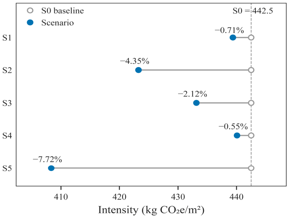
Each individual scenario reduced carbon emissions in Phases A1–A5, but the extent of the reductions varied significantly. The S2 scenario—low-carbon reinforcement—achieved the highest individual emission reduction of 731.39 tCO₂e, corresponding to a reduction rate of 4.35%; this was followed by the S3 scenario—optimized envelope materials—with a reduction rate of 2.12%. The emission reduction rates for the S1 structural concrete optimization and S4 transportation optimization scenarios were 0.71% and 0.55%, respectively.

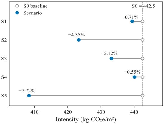
The emission reduction effects are compared in Figure 9. With the combined implementation of S1–S4, total carbon emissions under scenario S5 decreased to 15,514.70 tCO₂e, while the carbon emission intensity per unit floor area declined to 408.3 kgCO₂e/m². Compared with the baseline scenario, this represents a reduction of 1297.99 tCO₂e and an overall emission reduction rate of 7.72%. Among the individual scenarios, reinforcing steel optimization made the largest contribution to emission reduction, whereas transportation optimization had a relatively limited effect on total building carbon emissions.

Figure 9. A1–A5 carbon emissions and emission reduction effects under different low-carbon optimization scenarios.

Overall, the emission reduction scenario results confirmed the optimization priorities identified through hotspot identification and sensitivity analysis. Optimizing the parameters of high-contribution materials produced more substantial reductions in overall carbon emissions. By contrast, because the transportation stage accounted for only a small proportion of total emissions, optimizing this stage alone had a relatively limited effect on total carbon emissions.

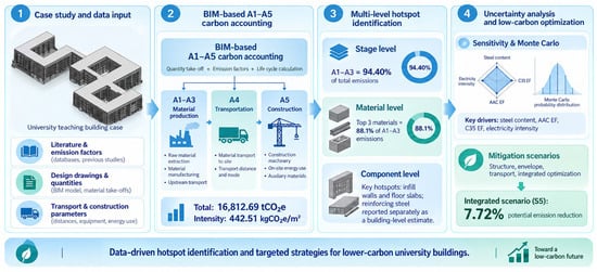
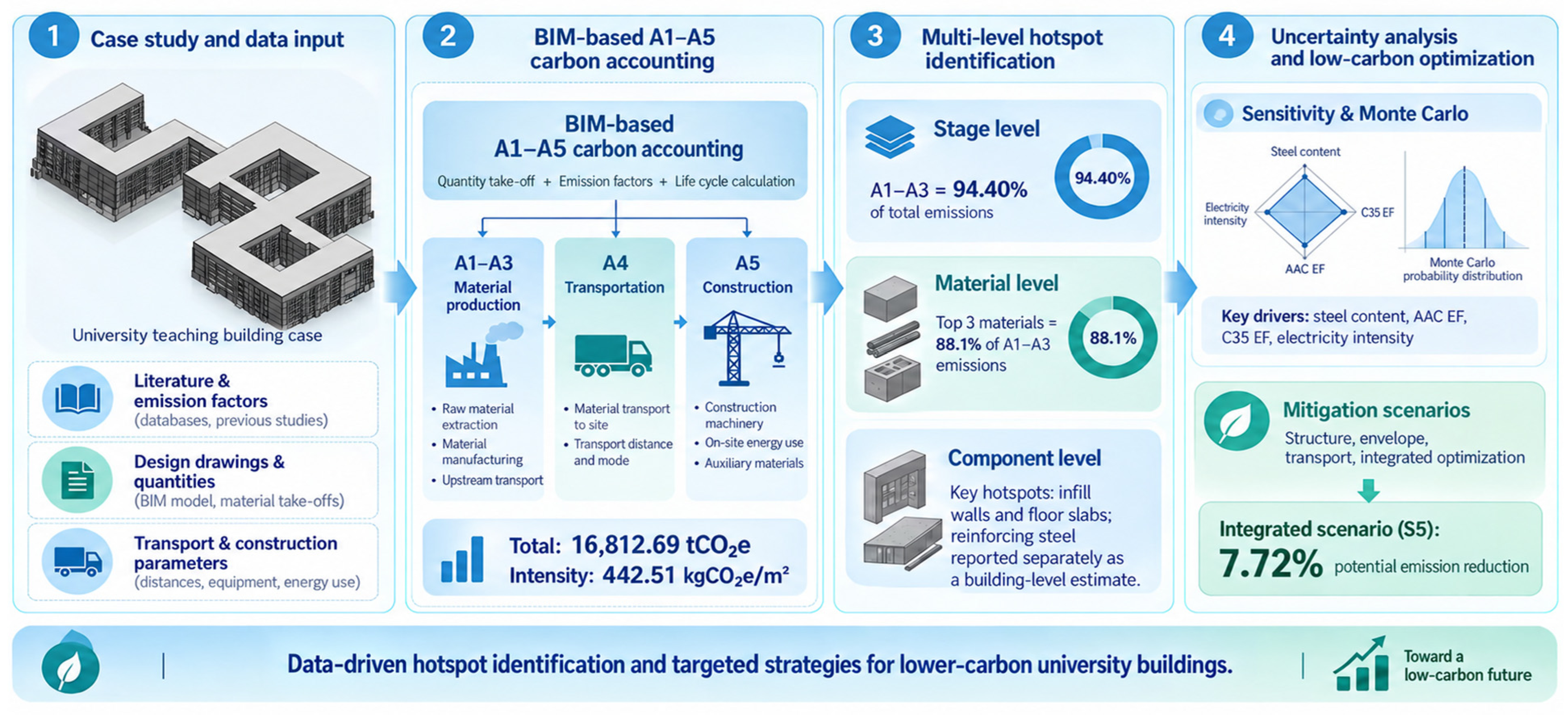
To clarify the relationships among multi-level carbon emission hotspot identification, key parameter analysis, and low-carbon scenario evaluation, Figure 10 provides an integrated overview of the main analytical procedures and findings of this study. It highlights the logical progression from identifying emission hotspots to selecting emission reduction measures and evaluating their potential emission reduction effects.

Figure 10. Integrated carbon emission analysis workflow and results.

4. Discussion

4.1. Multi-Level Carbon Emission Hotspots and Their Formation Mechanisms

This study identified carbon emission hotspots in the upfront stages of the teaching building at three levels: stage, material, and component. The results showed a pronounced concentration of emissions across all three levels: at the stage level, emissions were predominantly concentrated in the A1–A3 building material production stage; at the material level, they were mainly associated with C35 concrete, reinforcing steel, and autoclaved aerated concrete blocks; and at the component level, the major hotspots were reinforcing steel, infill walls, and floor slabs. Overall, the multi-level analysis identified clear priority stages, materials, and components for upfront carbon emission control, providing a basis for subsequent sensitivity analysis and the selection of low-carbon optimization targets.

From the perspective of hotspot formation, upfront carbon emissions are not determined by the characteristics of any single material, but rather by the combined effects of material quantities and unit carbon emission factors. In this case study, modules A1–A3 accounted for 94.4% of total A1–A5 emissions, while C35 concrete, reinforcing steel, and autoclaved aerated concrete blocks collectively contributed approximately 88.1%. Among these materials, concrete was used in large quantities, reinforcing steel had a relatively high carbon emission factor per unit mass, and autoclaved aerated concrete blocks accounted for a substantial amount of envelope work. Together, these three materials therefore constituted the principal emission hotspots. For reinforced-concrete public buildings with similar material systems, emission reduction efforts should prioritize the building material production stage and high-contribution materials rather than focusing solely on energy consumption at the construction site.

The integrated analysis across the stage, material, and component levels reveals how carbon emission sources are translated into physical building elements. High-contribution materials identified at the material level can be mapped, through BIM components, to specific building elements such as floor slabs and infill walls. In particular, the large volume of concrete used in floor slabs and the extensive use of masonry blocks in infill walls are major factors contributing to component-level hotspots. This indicates that building carbon emission hotspots are influenced not only by the emission characteristics of the materials themselves, but also by the scale of their use and their spatial distribution among different components. Compared with total-emission accounting or material ranking alone, multi-level hotspot identification can further trace overall emission contributions to specific physical objects that can be addressed through design, procurement, and construction control, thereby providing a clearer basis for subsequent material substitution, component optimization, and procurement management.

Comparison with relevant guidelines and educational building case studies showed that the main structural quantities and structural-system carbon emission intensity in this study were of a comparable order of magnitude, indicating that the case-study accounting results were reasonable at the engineering scale. After masonry blocks, exterior windows, and roofing materials were included, the A1–A3 carbon emission intensity increased markedly, indicating that building envelope materials may also constitute a non-negligible source of embodied carbon. For public buildings with substantial use of envelope materials, focusing only on primary structural materials such as concrete and reinforcing steel may underestimate the overall emission reduction requirements of the building material production stage. Therefore, structural and envelope materials should be considered in an integrated manner when controlling upfront carbon emissions rather than being treated separately.

4.2. Key Parameter Effects and Implications for Low-Carbon Emission Reduction

The key parameters considered in this study mainly included reinforcing steel content, carbon emission factors of major building materials, material transportation distances, and construction electricity and diesel consumption intensities. Variations in these parameters jointly affected the A1–A5 carbon emission accounting results and the effectiveness of low-carbon optimization.

Sensitivity analysis showed that reinforcing steel content, the carbon emission factors of major building materials, and construction electricity consumption intensity were important parameters affecting total A1–A5 carbon emissions, with material-related parameters exerting a more pronounced influence. This indicates that high-contribution materials not only determine the baseline emission level but also represent major sources of variation in the accounting results. In addition, although module A5 accounted for a relatively small proportion of total emissions, construction electricity consumption intensity still exhibited relatively high sensitivity. This suggests that the importance of a parameter should not be assessed solely on the basis of the emission share of the corresponding stage, but should also consider its range of variation and degree of uncertainty.

Monte Carlo simulation showed that when multiple parameters varied simultaneously, total carbon emissions remained concentrated around the baseline accounting result, while the ranking of the major material hotspots showed no substantial change. This indicates that, within the specified parameter ranges, the identification of key emission sources remained relatively stable. Reinforcing steel quantity, the carbon emission factors of major materials, and construction energy parameters remained the principal sources of uncertainty in total emissions. Because the reinforcing steel quantity, A4 transportation distance, and A5 construction energy parameters all involved estimated values, future engineering applications should prioritize improving the data quality of these parameters through design quantity schedules, procurement records, and on-site energy consumption records.

The low-carbon scenario analysis further demonstrated a clear relationship between emission reduction effects and the contribution levels of identified hotspots. Targeted optimization of high-contribution sources, such as reinforcing steel, concrete, and building envelope materials, achieved greater overall emission reductions than individual adjustments to the transportation stage. Under the integrated scenario, total A1–A5 carbon emissions were reduced by 7.72%. Therefore, similar buildings may benefit from an emission reduction pathway based on “hotspot identification–prioritization–integrated optimization.” It should be noted that the comprehensive optimization scenario does not explicitly account for potential interactions among different measures. In addition, material substitutions and adjustments to concrete grades must satisfy practical constraints, including structural safety, material availability, and project costs. Therefore, the scenario results primarily represent the potential emission reduction effects under the specified assumptions and conditions, rather than an optimized engineering solution that can be directly implemented in practice.

4.3. Research Limitations and Applicability

This study is subject to several limitations related to data availability and parameter assumptions. The BIM model did not include explicit reinforcing steel entities; therefore, the reinforcing steel quantity was estimated based on the steel content per unit floor area. The A4 transportation distance and A5 construction energy parameters also relied partly on empirical assumptions. Although sensitivity analysis and Monte Carlo simulation were used to quantify the effects of variations in these parameters, they cannot substitute for measured data or project-specific records. Therefore, the emission levels for stages A4 and A5, together with their relative contributions, should be interpreted as results obtained within the parameter ranges defined in this study. If more complete reinforcing steel schedules, material transportation records, and on-site energy consumption data become available, the uncertainty associated with empirical parameters could be reduced, and the accuracy of carbon emission accounting could be improved. In addition, the system boundary of this study covers only stages A1–A5 and does not include the building operation and maintenance stage, end-of-life processes, or benefits and loads beyond the system boundary. In future research, when data on building operation, maintenance, component replacement, demolition, and recycling become available, the assessment can be extended to cover carbon emissions across the entire building life cycle.

Due to limitations in the available data, some materials were excluded from the A1–A3 baseline calculation because corresponding production-stage carbon emission factors or independently quantified material quantities were unavailable. For materials without dedicated emission factors, such as glass curtain walls, proxy factors from similar materials were adopted. BIM–LCA studies commonly face data-related challenges involving emission factor matching and the completeness of material inventories [33]. Therefore, the results of this study represent the carbon emission level under the defined system boundary and the available material inventory, rather than the complete carbon footprint of all building materials. Materials excluded from the calculations may lead to an underestimation of total carbon emissions, with the magnitude of this underestimation depending on the types and quantities of omitted materials and their corresponding emission factors. The sensitivity analysis and Monte Carlo simulations conducted in this study primarily focus on the key parameters included in the carbon emission accounting and therefore cannot quantify the potential bias arising from the omission of certain materials. Future research could improve the regional applicability and matching accuracy of material emission factors by incorporating Environmental Product Declarations (EPDs), regional material databases, and measured data from project suppliers. The material scope, emission factor sources, and corresponding treatment procedures adopted in this study are provided in Appendix A.

From the perspective of methodological applicability, this study uses a single university teaching building with a reinforced concrete frame as a case study. The specific carbon emission values and hotspot rankings reflect the emission characteristics of this building under its particular material composition and construction conditions. The analytical workflow developed in this study is more suitable for individual teaching buildings with available BIM models or relatively complete bills of quantities, and is particularly applicable to reinforced concrete frame buildings with similar structural forms and material systems. For other building types, the analytical pathway of “quantity takeoff–emission factor matching–multi-level hotspot identification–uncertainty analysis–scenario optimization” can be retained, while the input parameters can be adjusted according to local material production conditions, transportation distances, electricity emission factors, and construction energy use. The methodological value of this study therefore lies primarily in the reusability of its analytical framework and decision-making logic rather than in the specific carbon emission values obtained for the case-study building.

At the engineering application level, this analytical workflow can also be integrated into the design, procurement, and construction management processes. During the design stage, alternative materials and construction schemes can be compared based on component-level hotspots. During the procurement stage, low-carbon procurement requirements can be established for high-contribution materials such as reinforcing steel, concrete, masonry blocks, and building envelope materials. During the construction stage, actual transportation and energy consumption data can be used to continuously update the A4–A5 accounting results. By further linking BIM-derived quantities with material environmental information, procurement records, and on-site energy data, one-time carbon emission accounting can gradually evolve into carbon management based on continuously updated project data, thereby enhancing the practical value of the proposed method for engineering decision-making.

5. Conclusions and Policy Implications

5.1. Conclusions

Based on BIM-derived quantity data, this study established an A1–A5 carbon emission accounting framework for a university teaching building, identified emission hotspots at the stage, material, and component levels, and comprehensively analyzed the key influencing factors and emission reduction potential through sensitivity analysis, Monte Carlo uncertainty analysis, and low-carbon scenario assessment. The main conclusions are as follows:

• Upfront carbon emissions were strongly concentrated in the building material production stage. For teaching buildings dominated by reinforced-concrete structures and masonry envelopes, the combined effects of material quantities and unit carbon emission factors make building material production the principal source of emissions. In this case study, modules A1–A3 accounted for 94.40% of total upfront carbon emissions. Concrete, reinforcing steel, and autoclaved aerated concrete blocks constituted the major material hotspots, indicating that emission reduction efforts for such buildings should not be limited to controlling on-site energy consumption during construction, but should also emphasize material selection and design optimization at the design stage.
• Multi-level analysis across the stage, material, and component levels can improve the hierarchy and specificity of carbon emission hotspot identification. Stage-level analysis identifies the major emission stages, material-level analysis determines high-contribution building materials, and component-level analysis further locates material hotspots within specific building elements such as floor slabs and infill walls. Compared with total-emission accounting or material ranking alone, this approach establishes a clearer correspondence between carbon emission sources and building design objects, thereby providing more specific targets for material substitution, component optimization, and procurement control.
• Parameters associated with high-contribution materials were also major sources of uncertainty in carbon emission accounting. Reinforcing steel content, the carbon emission factors of major building materials, and construction electricity consumption intensity showed relatively high sensitivity to total carbon emissions. Monte Carlo simulation indicated that, within the specified parameter ranges, the distribution of total emissions remained relatively concentrated and the ranking of the major material hotspots showed no substantial change, suggesting that hotspot prioritization was relatively stable. At the same time, key parameters such as reinforcing steel quantity, material carbon emission factors, and construction energy consumption should be prioritized in future efforts to improve data quality.
• Hotspot-based targeted optimization provides a more focused approach than uniformly allocating emission reduction measures. The scenario analysis confirmed the rationale for prioritizing optimization measures according to carbon emission hotspots and showed that the coordinated implementation of multiple emission reduction measures can improve the overall effectiveness of carbon emission reduction. In this case study, low-carbon reinforcing steel and building envelope material optimization produced relatively substantial emission reductions, while the integrated scenario reduced total A1–A5 carbon emissions by 7.72%. Therefore, similar buildings should adopt an emission reduction pathway based on “hotspot identification–prioritization–integrated optimization,” with priority given to high-contribution materials and key components while satisfying requirements for structural safety, material performance, and engineering feasibility.
• This study extends the application of BIM–LCA from carbon emission accounting to multi-level hotspot identification, uncertainty analysis, and low-carbon optimization assessment. Compared with studies focusing primarily on total-emission accounting, single-material analysis, or individual optimization measures, this study integrates BIM-derived quantities, stage–material–component hotspot identification, sensitivity and Monte Carlo uncertainty analyses, and emission reduction scenario assessment within a unified analytical workflow, forming an “accounting–identification–assessment–optimization” research chain. This approach not only quantifies upfront carbon emissions but also identifies priority targets for emission reduction and key uncertain parameters, thereby providing a methodological reference for low-carbon decision-making during the design, material selection, and construction stages of similar public buildings.

5.2. Policy Implications

Based on the above findings, low-carbon management of teaching buildings and similar public buildings should gradually shift from isolated control of construction-stage energy consumption toward coordinated management across the design, material procurement, and construction processes. During the design stage, BIM models can be used to establish a “component–material–emission factor” mapping relationship, allowing carbon emission assessment to be incorporated into material selection and construction scheme comparison, with priority given to high-contribution materials and key components. For major emission sources such as reinforcing steel, concrete, masonry blocks, and building envelope materials, the carbon emission differences associated with different material sources, production processes, and substitution options can be compared, provided that structural safety and building performance requirements are satisfied.

During the procurement stage, material carbon emission indicators can be progressively incorporated into supplier evaluation and procurement decision-making systems, while the use of building materials with Environmental Product Declarations (EPDs) or traceable carbon emission data should be encouraged. Compared with procurement decisions based solely on material cost and engineering performance, incorporating carbon emission indicators into material procurement assessment can enable emission reduction requirements to be implemented earlier in the material supply and procurement process. For high-contribution materials, priority should be given to establishing material carbon emission databases and dynamic updating mechanisms to provide a consistent data basis for comparing alternative solutions across different projects.

During the construction and project data management stages, process data on material transportation, construction electricity consumption, and fuel use should be systematically recorded and archived. Actual transportation distances and on-site energy consumption data should be progressively adopted to improve the accuracy of A4–A5 accounting parameters. By linking BIM-derived quantity data with procurement, transportation, and on-site energy records, the traceability of A4–A5 carbon emission accounting can be enhanced, while also providing a data basis for dynamic adjustment of carbon emission estimates during project implementation. For public buildings with similar material systems and construction methods, a carbon emission data management mechanism covering the design, procurement, and construction stages can be established accordingly, enabling building carbon emission assessment to extend from result-based accounting to design-stage scheme comparison and dynamic management during construction.

Appendix A.1 Monte Carlo Simulation and Probability Distribution

To evaluate the effects of input parameter variations on the A1–A5 carbon emission accounting results, key material, transportation, and construction energy parameters were selected for Monte Carlo uncertainty analysis based on the sensitivity analysis results. All parameters were assumed to be mutually independent and to follow triangular distributions:

X_i∼Tri(a_i,m_i,b_i)

(A1)

In the formula, X_i represents the i-th uncertain parameter, while a_i, m_i, and b_i denote the lower bound, mode, and upper bound of that parameter, respectively.

Monte Carlo simulation was performed using Python 3.12-based random sampling with 5000 iterations and a random seed of 20260825 to ensure reproducibility. The specific distribution ranges and parameter settings are presented in Table A1.

Appendix A.2 Input Parameters for Monte Carlo Simulation

Table A1. Input parameters and distribution settings for Monte Carlo simulation.

Parameter	Lower Bound	Mode	Upper Bound	Unit	Module
Reinforcing steel content	50	55	60	kg/m2	A1–A3
Carbon emission factor of C35 concrete	295	301.5	321	kgCO2e/m3	A1–A3
Carbon emission factor of autoclaved aerated concrete blocks	294.3	327	359.7	kgCO2e/m3	A1–A3
Carbon emission factor of exterior windows and curtain walls	194	224	254	kgCO2e/m2	A1–A3
Concrete transportation distance	10	20	40	km	A4
Reinforcing steel transportation distance	100	150	300	km	A4
Autoclaved aerated concrete block transportation distance	50	100	200	km	A4
Concrete wall transportation distance	10	30	40	km	A4
Insulation and waterproofing material transportation distance	100	200	400	km	A4
Exterior window and curtain wall transportation distance	200	300	500	km	A4
Door transportation distance	100	200	400	km	A4
Mortar transportation distance	20	50	80	km	A4
Construction electricity consumption intensity	20	30	40	kWh/m2	A5
Diesel consumption intensity	0.5	1.0	1.5	L/m2	A5

Table A1. Input parameters and distribution settings for Monte Carlo simulation.

Parameter	Lower Bound	Mode	Upper Bound	Unit	Module
Reinforcing steel content	50	55	60	kg/m2	A1–A3
Carbon emission factor of C35 concrete	295	301.5	321	kgCO2e/m3	A1–A3
Carbon emission factor of autoclaved aerated concrete blocks	294.3	327	359.7	kgCO2e/m3	A1–A3
Carbon emission factor of exterior windows and curtain walls	194	224	254	kgCO2e/m2	A1–A3
Concrete transportation distance	10	20	40	km	A4
Reinforcing steel transportation distance	100	150	300	km	A4
Autoclaved aerated concrete block transportation distance	50	100	200	km	A4
Concrete wall transportation distance	10	30	40	km	A4
Insulation and waterproofing material transportation distance	100	200	400	km	A4
Exterior window and curtain wall transportation distance	200	300	500	km	A4
Door transportation distance	100	200	400	km	A4
Mortar transportation distance	20	50	80	km	A4
Construction electricity consumption intensity	20	30	40	kWh/m2	A5
Diesel consumption intensity	0.5	1.0	1.5	L/m2	A5

Appendix A.3 Sources and Treatment of Material Carbon Emission Factors

Table A2. Sources and treatment methods of carbon emission factors for major materials.

Material	Source of Carbon Emission Factor	Treatment Method
C35 concrete	GB/T 51366—2019 and related material data	Linear interpolation based on the carbon emission factors of C30 and C50 concrete
HRB400 reinforcing steel	GB/T 51366—2019	Standard carbon emission factor directly adopted
Autoclaved aerated concrete blocks	GB/T 51366—2019/Guidelines for Carbon Emission Calculation of Civil Buildings in Jiangsu Province	Carbon emission factor corresponding to the relevant density grade adopted
XPS insulation board	Relevant material database	Calculated after converting volume to mass using material density
SBS waterproofing membrane	Relevant material database	Calculated based on material consumption per unit area
Exterior windows and curtain walls	Published research data	Carbon emission factor of thermally broken aluminum-framed windows adopted as a proxy
Doors	—	Excluded from the baseline calculation because no matching carbon emission factor was available

Table A2. Sources and treatment methods of carbon emission factors for major materials.

Material	Source of Carbon Emission Factor	Treatment Method
C35 concrete	GB/T 51366—2019 and related material data	Linear interpolation based on the carbon emission factors of C30 and C50 concrete
HRB400 reinforcing steel	GB/T 51366—2019	Standard carbon emission factor directly adopted
Autoclaved aerated concrete blocks	GB/T 51366—2019/Guidelines for Carbon Emission Calculation of Civil Buildings in Jiangsu Province	Carbon emission factor corresponding to the relevant density grade adopted
XPS insulation board	Relevant material database	Calculated after converting volume to mass using material density
SBS waterproofing membrane	Relevant material database	Calculated based on material consumption per unit area
Exterior windows and curtain walls	Published research data	Carbon emission factor of thermally broken aluminum-framed windows adopted as a proxy
Doors	—	Excluded from the baseline calculation because no matching carbon emission factor was available

Appendix A.4 Carbon Emission Factor Estimation and Conversion

For materials without directly matched carbon emission data, corresponding adjustments were made based on material grade, unit of measurement, and engineering application. The carbon emission factor of C35 concrete was determined by linear interpolation between the values for C30 and C50 concrete:

$$E{F}_{C35}=E{F}_{C30}+{\displaystyle \frac{35-30}{50-30}}\left(E{F}_{C50}-E{F}_{C30}\right)$$

(A2)

In the formula, EF_C35 represents the carbon emission factor of C35 concrete, while EF_C30 and EF_C50 denote the carbon emission factors of C30 and C50 concrete, respectively. The calculated carbon emission factor of C35 concrete was 301.50 kgCO₂e/m³.

The carbon emission factor of XPS insulation boards was expressed on a mass basis, whereas the BIM-derived quantity was measured by volume; therefore, the volume was converted to mass using the material density before calculation. Because a production-stage carbon emission factor that exactly matched the glass curtain wall system used in this project was unavailable, the carbon emission factor of thermally broken aluminum-framed windows was adopted as a proxy for the curtain wall, and this parameter was included in the Monte Carlo uncertainty analysis.

References

- Röck, M.; Saade, M.R.M.; Balouktsi, M.; Rasmussen, F.N.; Birgisdottir, H.; Frischknecht, R.; Habert, G.; Lützkendorf, T.; Passer, A. Embodied GHG emissions of buildings—The hidden challenge for effective climate change mitigation. Appl. Energy 2020, 258, 114107. [Google Scholar] [CrossRef] [Scilit]
- Huang, Z.; Zhou, H.; Miao, Z.; Tang, H.; Lin, B.; Zhuang, W. Life-Cycle Carbon Emissions (LCCE) of Buildings: Implications, Calculations, and Reductions. Engineering 2024, 35, 115–139. [Google Scholar] [CrossRef] [Scilit]
- De Wolf, C.; Pomponi, F.; Moncaster, A. Measuring embodied carbon dioxide equivalent of buildings: A review and critique of current industry practice. Energy Build. 2017, 140, 68–80. [Google Scholar] [CrossRef] [Scilit]
- Hawkins, D.; Mumovic, D. Evaluation of life cycle carbon impacts for higher education building redevelopment: An archetype approach. Energy Build. 2017, 147, 113–122. [Google Scholar] [CrossRef] [Scilit]
- Zhao, Z.; Pan, C.; Yang, G.; Ji, C.; Massucato, C.J.; Attia, S. Establishing industry-based benchmarks for embodied carbon in buildings: A statistical analysis of 85 case studies in China. J. Build. Eng. 2025, 114, 114372. [Google Scholar] [CrossRef] [Scilit]
- Feng, H.; Luo, W.; Wang, J.; Wu, P. A quantitative method and application of carbon reduction effect for campus based on the whole life cycle. Guangdong Archit. Civ. Eng. 2022, 29, 1–5. (In Chinese) [Google Scholar] [CrossRef]
- Kanafani, K.; Magnes, J.; Lindhard, S.M.; Balouktsi, M. Carbon emissions during the building construction phase: A comprehensive case study of construction sites in Denmark. Sustainability 2023, 15, 10992. [Google Scholar] [CrossRef] [Scilit]
- Teng, Y.; Xu, J.; Pan, W.; Zhang, Y. A systematic review of the integration of building information modeling into life cycle assessment. Build. Environ. 2022, 221, 109260. [Google Scholar] [CrossRef] [Scilit]
- Li, Z.; Wang, Y.; Chen, Y.; Zhang, H.; Jiang, L. Application of BIM for carbon reduction across the whole life cycle of buildings via bibliometric analysis. J. Tsinghua Univ. Sci. Technol. 2025, 65, 1239–1249. (In Chinese) [Google Scholar] [CrossRef]
- Xu, Y.; Gong, X.; Tao, X.; Kwok, H.H.L.; Limsawasd, C.; Cheng, J.C.P. Automated openBIM-based discrete event simulation modeling for cradle-to-site embodied carbon assessment. Autom. Constr. 2025, 175, 106217. [Google Scholar] [CrossRef] [Scilit]
- Yuan, H.; Huang, B.; Wang, M.; Tang, Y.; Mao, J.; Xiong, L. BIM-enabled lifecycle carbon emission management integrating multi-physical field steady-state methods during operation. Autom. Constr. 2026, 181, 106683. [Google Scholar] [CrossRef] [Scilit]
- Liang, B.; Zhou, J.; Wu, D. Research on building carbon emission estimation and emission reduction strategies driven by BIM technology. Urban Archit. 2025, 22, 108–110. (In Chinese) [Google Scholar] [CrossRef]
- Di Ruocco, G.; Genovese, V. EPBD IV: Decarbonization Strategies Through a BIM-LCA Workflow—Case Study of a Crèche Design in Montoro, Southern Italy. Buildings 2026, 16, 3547. [Google Scholar] [CrossRef] [Scilit]
- Feng, H.; Zhao, J.; Zhang, H.; Zhu, S.; Li, D.; Thurairajah, N. Uncertainties in whole-building life cycle assessment: A systematic review. J. Build. Eng. 2022, 50, 104191. [Google Scholar] [CrossRef] [Scilit]
- Li, J.; Lützkendorf, T.; Balouktsi, M.; Bi, X.; Alaux, N.; Potrč Obrecht, T.; Passer, A.; Han, C.; Yang, W. Identifying uncertainties in the whole life carbon assessment of buildings: Sources, types, and potential actions. Build. Environ. 2023, 244, 110779. [Google Scholar] [CrossRef] [Scilit]
- Robati, M.; Daly, D.; Kokogiannakis, G. A method of uncertainty analysis for whole-life embodied carbon emissions of building materials of a net-zero energy building in Australia. J. Clean. Prod. 2019, 225, 541–553. [Google Scholar] [CrossRef] [Scilit]
- Gauch, H.L.; Dunant, C.F.; Hawkins, W.; Cabrera Serrenho, A. What really matters in multi-storey building design? A simultaneous sensitivity study of embodied carbon, construction cost, and operational energy. Appl. Energy 2023, 333, 120585. [Google Scholar] [CrossRef] [Scilit]
- Kathiravel, R.; Feng, H. Structural and embodied carbon performance optimization for low carbon buildings through BIM-based integrated design. J. Build. Eng. 2024, 98, 111008. [Google Scholar] [CrossRef] [Scilit]
- Mergos, P.E. Structural design of reinforced concrete frames for minimum amount of concrete or embodied carbon. Energy Build. 2024, 318, 114505. [Google Scholar] [CrossRef] [Scilit]
- Lyu, Y.; Fomin, N.I.; Li, S.; Hu, W.; Xiao, S.; Huang, Y.; Liu, C. Life cycle carbon emission analysis of buildings with different exterior wall types based on BIM technology. Buildings 2025, 15, 138. [Google Scholar] [CrossRef] [Scilit]
- Shi, Y.; Yang, Z.; Zheng, S.; Gao, D.; Yang, X. Multi-objective optimization of embodied carbon emission, energy consumption, and daylighting performance of educational building in the schematic design stage. J. Build. Eng. 2025, 106, 112594. [Google Scholar] [CrossRef] [Scilit]
- Fang, D.; Brown, N.; De Wolf, C.; Mueller, C. Reducing embodied carbon in structural systems: A review of early-stage design strategies. J. Build. Eng. 2023, 76, 107054. [Google Scholar] [CrossRef] [Scilit]
- ISO 14040:2006; Environmental Management—Life Cycle Assessment—Principles and Framework. ISO: Geneva, Switzerland, 2006.
- ISO 14044:2006; Environmental Management—Life Cycle Assessment—Requirements and Guidelines. ISO: Geneva, Switzerland, 2006.
- EN 15978:2011; Sustainability of Construction Works—Assessment of Environmental Performance of Buildings—Calculation Method. CEN: Brussels, Belgium, 2011.
- GB/T 51366—2019; Standard for Building Carbon Emission Calculation. China Architecture & Building Press: Beijing, China, 2019. (In Chinese)
- Department of Housing and Urban-Rural Development of Jiangsu Province. Guidelines for Carbon Emission Calculation of Civil Buildings in Jiangsu Province; Su Jian Ke 【2023】No. 153; Department of Housing and Urban-Rural Development of Jiangsu Province: Nanjing, China, 2023. (In Chinese)
- EN 15804:2012+A2:2019; Sustainability of Construction Works—Environmental Product Declarations—Core Rules for Construction Products. CEN: Brussels, Belgium, 2019.
- Greer, F.; Horvath, A. Exploring the significance of transportation emissions in upfront embodied carbon in buildings. Build. Environ. 2025, 269, 112457. [Google Scholar] [CrossRef] [Scilit]
- Kushwaha, A.S.; Mahindrakar, A.B. Assessment of global warming potential from on-site construction processes (module A5): A pilot building case study. Front. Built Environ. 2026, 12, 1769414. [Google Scholar] [CrossRef] [Scilit]
- Zhongshan Housing and Urban-Rural Development Bureau. Case-Based Cost Indicators for Construction Projects in Zhongshan (2023); Zhongshan Housing and Urban-Rural Development Bureau: Zhongshan, China, 2023. (In Chinese)
- Gillott, C.; Lanau, M.; Mitchell Reid, E.; Sharmin, F.; Densley Tingley, D. Material stocks and embodied carbon in UK buildings: An archetype-based, bottom-up, GIS approach. J. Ind. Ecol. 2025, 29, 1748–1762. [Google Scholar] [CrossRef] [Scilit] [PubMed]
- Berges-Alvarez, I.; Martínez-Rocamora, A.; Marrero, M. A systematic review of BIM-based life cycle sustainability assessment for buildings. Sustainability 2024, 16, 11070. [Google Scholar] [CrossRef] [Scilit]
Disclaimer/Publisher’s Note: The statements, opinions and data contained in all publications are solely those of the individual author(s) and contributor(s) and not of MDPI and/or the editor(s). MDPI and/or the editor(s) disclaim responsibility for any injury to people or property resulting from any ideas, methods, instructions or products referred to in the content. |
© 2026 by the authors. Licensee MDPI, Basel, Switzerland. This article is an open access article distributed under the terms and conditions of the Creative Commons Attribution (CC BY) license.