Identification of Natural Frequencies and Damping Ratios of Brick-Concrete Structural Buildings Under Blasting Vibration Excitation

Abstract

The identification of natural frequencies and damping ratios in brick-concrete structures subjected to blasting vibrations is a critical prerequisite for stability analysis. However, results from a single modal identification method exhibit considerable errors and do not address uncertainty. This study proposes a multi-domain collaborative and clustering fusion (MDCCF) approach, validated through numerical simulations. Building on this foundation, we conducted vibration monitoring and candidate frequency/damping ratio identification for brick-concrete structures under deep-hole blasting in open-pit mines, followed by probabilistic distribution analysis of the identified parameters. Results demonstrate that the MDCCF method achieves higher accuracy than covariance-driven stochastic subspace identification (SSI-cov)-K-means and peak-picking (PP)-K-means methods, with candidate natural frequencies and damping ratios more closely approximating theoretical values. The ten candidate natural frequencies of the structure under deep-hole blasting were identified as 7.69 Hz, 10.559 Hz, 17.2068 Hz, 22.095 Hz, 27.099 Hz, 29.7741 Hz, 34.668 Hz, 40.039 Hz, 48.7882 Hz and 50.6476 Hz, with corresponding candidate damping ratios of 4.4602%, 3.705%, 2.8618%, 2.4161%, 1.9%, 1.45%, 1.11%, 0.8579%, 0.59% and 0.3493%. The natural frequencies and damping ratios of brick-concrete structures exhibit strong normal and Gamma distribution characteristics, respectively. Bootstrap analysis was further employed to quantify the statistical uncertainty of the identified natural frequencies and damping ratios, and the corresponding 95% confidence intervals were obtained. The identified frequency groups are interpreted as candidate modal frequencies rather than definitively confirmed global structural modes.

1. Introduction

In rock excavation operations, blasting is often unavoidable. It is not only prevalent in mining but also widely employed in projects such as tunnel, subway, highway, and dam construction. Blasting technology offers advantages like high construction efficiency and significant economic benefits, but it also brings negative impacts, such as ground vibration, air shock waves, and flying rocks [1,2,3]. Among these, blasting-induced ground vibration constitutes a severe environmental issue requiring urgent resolution [4,5]. In China, some buildings surrounding blast zones are brick-concrete structures. The ground vibration induced by blasting can adversely affect their stability, necessitating urgent research.

Explosion-induced vibrations can cause varying degrees of damage to surrounding buildings, adversely affecting their stability [6]. When assessing blast-induced structural damage, two critical factors are particle peak velocity (PPV) and dominant frequency [7,8]. Excessively high PPV values may lead to localized or overall structural damage. When the dominant frequency of the blasting vibration wave is close to the natural frequency of a structure, it can cause resonance in the building, thereby amplifying the PPV. Buildings with low damping ratios exhibit heightened sensitivity to prolonged vibrations and are prone to resonance [9,10]. Therefore, accurate identification of a building’s natural frequency and damping ratio is essential for precise evaluation of blast vibration effects on structural stability.

The natural frequency, damping ratio, and modal shape of a building are collectively referred to as modal parameters. To determine a building’s natural frequency and damping ratio, modal identification is required [11]. Modal identification refers to the process of extracting modal parameters from structural vibration data. The methods primarily include input–output and output-only approaches. The latter, due to its practicality and convenience, has gained significant attention and can be categorized into three types: frequency-domain methods, time-frequency-domain methods, and time-domain approaches [12,13]. Frequency-domain methods mainly include peak-picking (PP) methods [14] and frequency-domain decomposition (FDD) methods [15]. PP methods provide a simple and rapid means of identifying dominant spectral peaks, although their performance may be limited when closely spaced modes are present. FDD methods improve the separation of structural modes and are effective for identifying modal frequencies and mode shapes, while damping ratio estimation may require further refinement. Since blasting excitation is impulsive, the resulting structural response is transient and inherently non-stationary. Time-frequency analysis therefore provides an important means of characterizing the temporal evolution of frequency components in such responses. Representative methods include STFT [16], the WV distribution [17], WT [18], and HHT [19]. These methods are generally non-parametric and do not require an explicit parametric model of the structural system [20]. Conventional implementations nevertheless exhibit specific limitations, including the time-frequency resolution trade-off of STFT, cross-term interference in the WV distribution, wavelet-basis dependence in WT, and mode mixing and endpoint effects in HHT. Advanced techniques, such as reassignment, synchrosqueezing, and the Stockwell transform [21], can provide improved time-frequency localization and enhanced characterization of transient signals. these method-specific limitations do not imply that time-frequency analysis is unsuitable for blast-induced structural responses. In the present study, the objective is to obtain representative natural frequencies from multiple blasting records for subsequent statistical analysis, rather than to resolve the instantaneous frequency evolution during each blasting event. For this purpose, time-domain modal identification methods provide a suitable framework. Time-domain approaches include the random decrement technique [13,22] and stochastic subspace identification (SSI) method [23]. Among these, the SSI method has gained significant attention in recent years due to its robust mathematical foundation, high precision, and robustness, and has been widely applied in the field of building modal parameter identification [24,25,26]. The SSI method in modal identification operates as follows: first, a state-space model is established based on the dynamic response of the target structure, and then the modal parameters are estimated using the output matrix and state matrix of this model [27]. The method primarily comprises two approaches: covariance-driven stochastic subspace identification (SSI-cov) and data-driven stochastic subspace identification (SSI-data) [28]. Proper selection of custom parameters is critical for SSI algorithms, as different parameter choices can lead to significant variations in modal parameter identification. Particularly in continuous modal tracking, multiple adjustments of these parameters are required to achieve optimal results for each dataset. Automated interpretation of stabilization diagrams and clustering of stable poles have been extensively investigated in previous studies [29,30]. Magalhães et al. developed an automatic modal identification procedure combining SSI-COV with hierarchical clustering, while Reynders et al. proposed a fully automated three-stage clustering framework for stabilization-diagram interpretation. Each of the above methods has its advantages and limitations. When identifying modal parameters of brick-concrete structures subjected to blasting vibrations, uncertainties such as material inhomogeneity and structural complexity often introduce a degree of variability in the identified natural frequencies and damping ratios. This issue is not addressed by the aforementioned methods. Furthermore, the transient and high-energy nature of blasting vibration signals may render the reliability of any single method insufficient. In recent years, cluster analysis has been widely applied in data analysis to effectively identify characteristic parameters [31,32]. Therefore, this study integrates a time-domain modal identification method and a frequency-domain modal identification method, followed by clustering-based fusion analysis of the identified modal parameters. This approach enhances the reliability and robustness of modal parameter identification for brick-concrete structures subjected to blasting vibrations while addressing associated uncertainties.

This study poses a modal parameter identification method based on a framework integrating data evaluation, multi-domain identification, and clustering fusion. The proposed method is validated through numerical simulations. Following successful validation, vibration monitoring of brick-concrete structures under open-pit deep-hole blasting was performed, achieving accurate identification of their modal parameters. Subsequent probability distribution analysis of these parameters further confirms the method’s reliability.

2. MDCCF Modal Parameter Identification Method

2.1. PP Method

The PP method is a frequency-domain approach for structural modal parameter identification. By analyzing measured input–output signals, it calculates the frequency response function through integral transformation. This method directly determines a structure’s natural frequencies and damping ratios in the frequency domain by correlating the frequency response function with modal parameters. However, under blasting vibration conditions, obtaining accurate input signals becomes challenging, making precise frequency response function acquisition difficult. Since the power spectral density function of external excitation loads closely resembles the frequency response function, structural modal parameters can be identified through peak values in the power spectral density curve of response signals. The workflow for modal parameter identification using the power spectrum peak method is illustrated as follows [14]:

(1)

Sensors are arranged at key positions on the structure to collect the structural response signals under the external excitation. In order to avoid the phenomenon of frequency confusion, the sampling frequency should be no less than twice the cutoff frequency according to the Nyquist sampling theorem.

(2)

Calculate the power spectral density at different measurement points. If multiple measurement points are available, the power spectral densities from all points can be synthesized into an averaged normalized power spectral density, which is then used to identify structural modal parameters through its peak values. The power spectral modal decomposition form and the averaged normalized power spectral density are, respectively, given by (Equations (1) and (3)).

$$S_{\mathit{xx}}(\omega )=\mathrm{H}(j\omega )S_{ff}(\omega ){\mathrm{H}}^{\mathrm{H}}(j\omega )$$

(1)

where $S_{\mathit{xx}}(\omega )$ is the power spectral density matrix of the structural responses, $S_{ff}(\omega )$ is the power spectral density matrix of the excitation, H(jω) is the frequency response function matrix, and the superscript $\mathrm{H}$ denotes the conjugate transpose.

For multiple measurement points, the PSD of each response channel is first normalized over the investigated frequency range:

$${\mathit{NPSD}}_i(f_k)={\displaystyle \frac{{\mathit{PSD}}_i(f_k)}{{\sum }_{r=1}^{N_f}{\mathit{PSD}}_i(f_r)}}$$

(2)

The averaged normalized power spectral density is then obtained as

$$\mathit{ANPSD}(f_k)={\displaystyle \frac{1}{m}}{\sum }_{i=1}^m{\mathit{NPSD}}_i(f_k)$$

(3)

where m is the number of measurement points and ${\mathrm{N}}_{\mathrm{f}}$ is the number of discrete frequency bins.

(3)

Calculate the transfer function and its corresponding phase angle, and filter real and false structural modal parameters based on whether the phase angle is near 0° or 180° (±30°). The transmissibility between the target channel $p$ and the reference channel $q$ is defined as (Equation (4)):

$$T_{pq}(w)={\displaystyle \frac{{\mathrm{X}}_{\mathrm{p}}(w)}{{\mathrm{X}}_{\mathrm{q}}(w)}}$$

(4)

where ${\mathrm{X}}_{\mathrm{p}}(\mathrm{w})$ and ${\mathrm{X}}_{\mathrm{q}}(\mathrm{w})$ are the Fourier transforms of the responses at the target and reference measurement points, respectively.

(4)

The PP method was used to identify candidate natural frequencies, while the damping ratios were estimated from the free-decay responses extracted using the random decrement technique (RDT) [33]. The RDT procedure suppresses the random excitation component through ensemble averaging and yields an approximately free-decay response, from which the damping ratio can subsequently be estimated.

2.2. SSI-Cov Method

The SSI method is a widely used and highly accurate approach for identifying structural modal parameters in the time domain. This method extracts modal parameters from the structure’s output response signals under unknown external excitation inputs. It primarily includes two variants: SSI-cov and SSI-data. Compared to SSI-data, SSI-cov demonstrates superior numerical stability, robust noise resistance, and higher reliability and reproducibility of identification results. The workflow for SSI-cov to identify structural modal parameters is outlined below [28,30]:

(1)

Construct the Hankel matrix

The block Hankel matrix is constructed from the measured output responses. Let $y_k\in {\mathrm{R}}^l$ denote the $l$-channel output vector at the $k$-th sampling instant. The past and future output matrices, $Y_p$ and $Y_f$, are defined as Equation (5).

$$Y=\left({\displaystyle \frac{Y_p}{Y_f}}\right)={\displaystyle \frac{1}{\sqrt{j}}}\left[{\displaystyle \frac{\begin{array}{ccccc}{y}_0& y_1& y_2& \dots & y_{j-1}\\ y_1& y_2& y_3& \dots & y_j\\ \dots & \dots & \dots & \ddots & ⋮\\ y_{i-1}& y_i& y_{i+1}& \dots & y_{i+j-2}\end{array}}{\begin{array}{ccccc}{y}_i& y_{i+1}& {y_{i+}}_2& \dots & y_{i+j-1}\\ y_{i+1}& y_{i+2}& y_{i+3}& \dots & y_{i+j}\\ \dots & \dots & \dots & \ddots & ⋮\\ y_{2i-1}& y_{2i}& y_{2i+1}& \dots & y_{2i+j-2}\end{array}}}\right]$$

(5)

(2)

Construct the Toeplitz matrix

In the SSI-COV method, the structural modal parameters are identified from the covariance matrices of the measured output responses. Based on the past and future output matrices defined above, the first block Toeplitz matrix is constructed as

$$T_{1\left|i\right.}=Y_f{Y_p}^T=\left[\begin{array}{cccc}{R}_i& R_{i-1}& \dots & R_1\\ R_{i+1}& R_i& \dots & R_2\\ \dots & \dots & \ddots & ⋮\\ R_{2i-1}& R_{2i-2}& \dots & R_i\end{array}\right]$$

(6)

where ${\mathrm{R}}_i$ denotes the output covariance matrix at time lag $i$. To construct the one-step-shifted Toeplitz matrix, the future output matrix is shifted forward by one sampling interval and denoted by ${\mathrm{Y}}_{\mathrm{f}}^{+}$. The corresponding Toeplitz matrix is then expressed as

$${\mathrm{Y}}_f^{+}={\displaystyle \frac{1}{\sqrt{j}}} \left[\begin{array}{cccc}{y}_{i+1}& y_{i+2}& \dots & y_{i+j}\\ y_{i+2}& y_{i+3}& \dots & y_{i+j+1}\\ \dots & \dots & \ddots & ⋮\\ y_{2i}& y_{2i+1}& \dots & y_{2i+j-1}\end{array}\right]$$

(7)

$$T_{2\left|i+1\right.}={\mathrm{Y}}_f^{+}{Y_p}^T=\left[\begin{array}{cccc}{R}_{i+1}& R_i& \dots & R_2\\ R_{i+2}& R_{i+1}& \dots & R_3\\ \dots & \dots & \ddots & ⋮\\ R_{2i}& R_{2i-1}& \dots & R_{i+1}\end{array}\right]$$

(8)

Here, ${\mathrm{Y}}_{\mathrm{f}}^{+}$ is obtained by shifting ${\mathrm{Y}}_{\mathrm{f}}$ forward by one sampling instant. Therefore, ${\mathrm{T}}_{1\left|\mathrm{i}\right.}$ and ${\mathrm{T}}_{2\left|\mathrm{i}+1\right.}$ contain covariance information at two consecutive sets of time lags and are subsequently used to estimate the system state matrix.

Assuming the response y_k undergoes various states, the output covariance can be expressed as (Equation (9)):

$$R_k={\displaystyle \frac{1}{j}}\sum y_{r+k}{y}_r^T$$

(9)

During the field testing process, due to the limited number of measurement points, the output covariance estimate can be expressed as (Equation (10)):

$${\widehat{R}}_i={\displaystyle \frac{1}{j}}{\sum }_{k=0}^{j-1}{y}_{k+i}{y}_k^T$$

(10)

Substitute (Equation (10)) into (Equation (6)), and then perform matrix T factorization to obtain (Equation (11)).

$$T_{1\left|i\right.}=\left[\begin{array}{c}C\\ \mathrm{CA}\\ \cdots \\ C{A}^{i-1}\end{array}\right]\left[\begin{array}{c}\begin{array}{cccc}{A}^{i-1}G\hspace{1em}& \cdots \hspace{1em}& \mathrm{AG}\hspace{1em}& G\end{array}\end{array}\right]=O_i{\mathsf{\Gamma }}_i$$

(11)

where O_i is an observable matrix, $O_i=U_1{S}_1^{1/2}$, and Γ_i is a controllable matrix, ${\mathsf{\Gamma }}_I=S_1^{1/2}{V}_1^T$.

(3)

Toeplitz matrix decomposition

Factorize the Toeplitz matrix as shown below (Equation (12)):

$$T_{1\left|i\right.}=\mathrm{US}{V}^T=\left[U_1 U_2\right]\left[\begin{array}{cc}{S}_1& 0\\ 0& 0\end{array}\right]\left[\begin{array}{c}{V_1}^T\\ {V_2}^T\end{array}\right]=U_1{S}_1{V_1}^T$$

(12)

where S₁ is a diagonal matrix with singular values in descending order, U is an orthogonal matrix, U^TU = I, and V^TV = I is an orthogonal matrix.

(4)

Solve the state matrix

Construct the next time-delay covariance T_2|i+1 matrix in T_1|i matrix form, with the matrix expression as (Equation (13)):

$$T_{2\left|i+1\right.}=\left[\begin{array}{c}\mathrm{CA}\\ C{A}^2\\ \cdots \\ C{A}^i\end{array}\right]\left[\begin{array}{c}\begin{array}{cccc}{A}^{i-1}G& \cdots & \mathrm{AG}& G\end{array}\end{array}\right]=O_{i}A{\mathsf{\Gamma }}_i$$

(13)

The output matrix consists of the first l rows of the observable matrix, and the state matrix can be expressed as (Equation (14)):

$$A=O_i^{+}{T}_{2/i+1}{\mathsf{\Gamma }}_i^{+}=S_1^{-1/2}{U}_1^T{T}_{2/i+1}{V}_1{S}_1^{-1/2}$$

(14)

(5)

Structural modal parameter identification

The eigenvalue decomposition of the identified discrete-time state matrix can be expressed as (Equation (15)):

$$A=\psi D{\psi }^{-1}$$

(15)

where D is a diagonal matrix containing the discrete-time eigenvalues ${\mu }_{\mathrm{i}}$, and ψ is the corresponding eigenvector matrix. The discrete-time eigenvalues are converted into continuous-time poles according to

$${\lambda }_{c,i}={\displaystyle \frac{ln({\mu }_i)}{∆t}}$$

(16)

where $∆t$ is the sampling interval. The natural frequency $f_i$ and damping ratio ${\xi }_i$ of the ith mode are then calculated as

$$f_i={\displaystyle \frac{1}{2\pi }}\sqrt{{\left[\mathrm{R}\mathrm{e}({\lambda }_{c,i})\right]}^2+{\left[\mathrm{I}\mathrm{m}({\lambda }_{c,i})\right]}^2}$$

(17)

$${\xi }_i=-{\displaystyle \frac{\mathrm{R}\mathrm{e}({\lambda }_{c,i})}{\left|{\lambda }_{c,i}\right|}}=-{\displaystyle \frac{\mathrm{R}\mathrm{e}({\lambda }_{c,i})}{\sqrt{{\left[\mathrm{R}\mathrm{e}({\lambda }_{c,i})\right]}^2+{\left[\mathrm{I}\mathrm{m}({\lambda }_{c,i})\right]}^2}}}$$

(18)

where $\mathrm{R}\mathrm{e}({\lambda }_{\mathrm{c},\mathrm{i}}$) and $\mathrm{I}\mathrm{m}({\lambda }_{\mathrm{c},\mathrm{i}})$ denote the real and imaginary parts of the ith continuous-time pole, respectively.

2.3. MDCCF Method

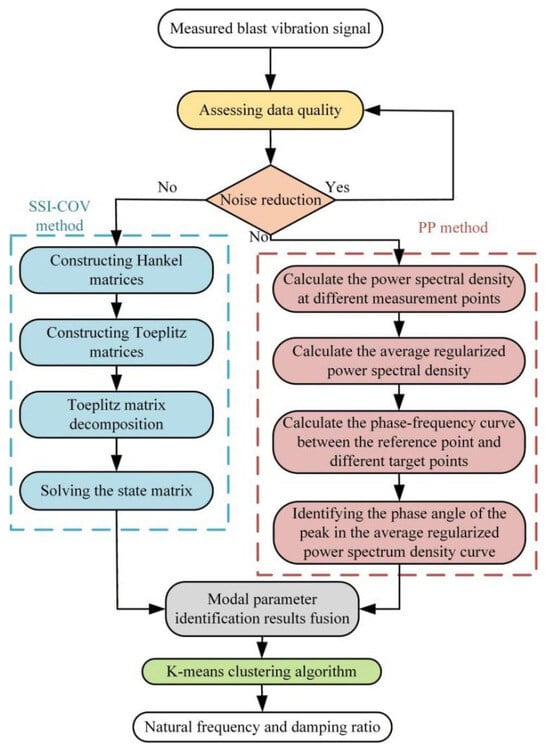
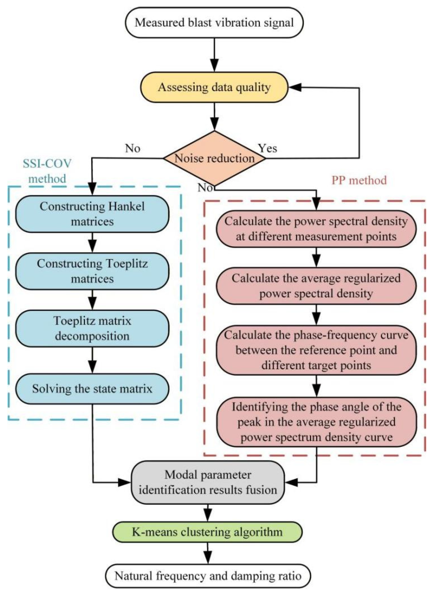
To enhance the reliability and robustness of modal parameter identification for brick-concrete structures under blasting vibration, this study proposes a novel method integrating multi-domain collaboration and clustering fusion, based on a data evaluation, multi-domain identification, clustering fusion framework. The approach employs exploratory data analysis to assess response signal quality, combines time-domain SSI-cov and frequency-domain PP methods for candidate modal parameter extraction, and utilizes clustering analysis to identify true structural modal parameters. The MDCCF method is illustrated in Figure 1.

Figure 1. The MDCCF method.

The MDCCF method steps are as follows:

(1)

The measurement points are selected according to the research object, and divided into one reference point and several target points. The sensors are set up at the measurement points to collect the blasting vibration signals. The data quality of the blasting vibration signals at different monitoring points is evaluated by the histogram and the correlation analysis diagram.

(2)

If the blasting vibration signal has obvious noise, the noise is reduced, otherwise, the PP method and SSI-cov method are used to identify the modal parameters of the structure directly.

(3)

Initialize the parameters of the SSI-cov method, construct the Hankel matrix and calculate the Toeplitz matrix, decompose the Toeplitz matrix into singular values, decompose the eigenvalues of the state matrix, set the tolerance of the natural frequency and damping ratio to 1% and 5%, respectively, output the stability diagram and define the identification result as modal parameter 1.

(4)

On the basis of calculating the power spectrum density function of blasting vibration signals at different measurement points, the average normalized power spectrum density and the phase angle of the transfer function are obtained. The average normalized power spectrum peak value is the natural frequency, which is checked by the phase angle of the transfer function. The identification result is defined as modal parameter 2.

(5)

The K-means algorithm is applied to cluster the modal parameters 1 and 2. Prior to clustering, the natural-frequency and damping ratio features are standardized using z-score normalization to eliminate the effects of different physical dimensions and numerical scales. The optimal number of clusters is determined from the variation in the sum of squared errors (SSE) with K using the elbow criterion [34]. Manhattan distances from the standardized modal parameters to the cluster centers are then calculated for classification. When the cluster centers no longer change, the clustering process is considered converged, and the final cluster centers are taken as the identified modal parameters.

3. Numerical Simulation Verification of the MDCCF Method

3.1. Establishment of the Numerical Model of the Frame Structure

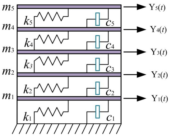
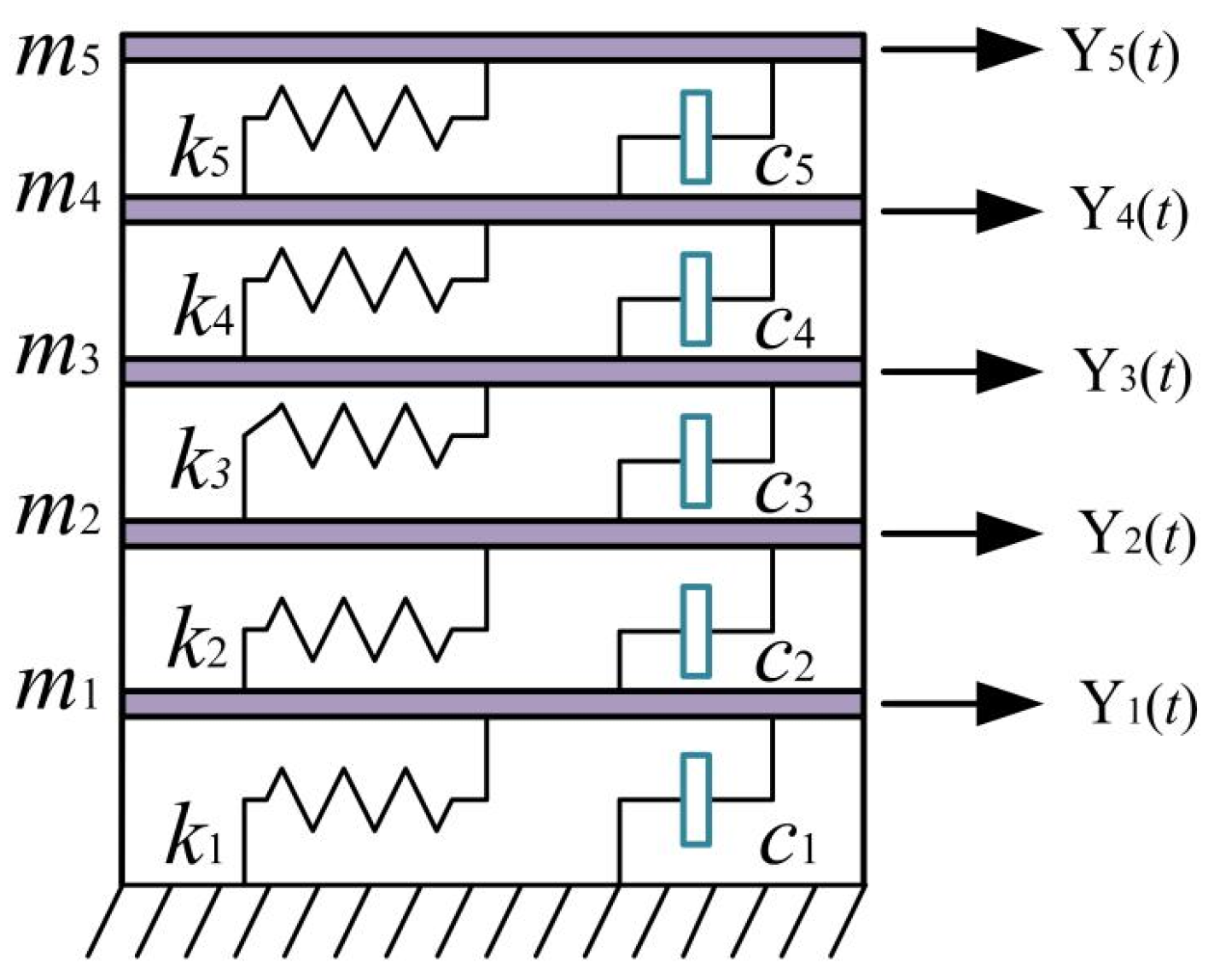
To validate the feasibility and accuracy of the MDCCF method, a five-story frame structure numerical model is used as a case study. As shown in Figure 2, the damping of this numerical model is Rayleigh damping. The mass of each story is m₁ = m₂ = m₃ = m₄ = m₅ = 500t, and the inter-story stiffness is k₁ = k₂ = k₃ = k₄ = k₅ = 3 × 10⁵ kN/m.

Figure 2. Numerical model of the five-storey frame structure.

Random white noise [35] velocity excitations were applied as environmental excitation to each story to obtain the velocity responses at different levels. The environmental excitation consisted of 15 cycles, with a sampling frequency of 1000 Hz and a sampling duration of 5 s. Figure 3 shows the white-noise velocity excitation applied to the first story. The velocity time-history curves for the stories are shown in Figure 4.

Figure 3. Time history of the white-noise velocity excitation applied to the first story.

Figure 4. Velocity time-history curves for different stories. (a) First story. (b) Second story. (c) Third story. (d) Fourth story. (e) Fifth story.

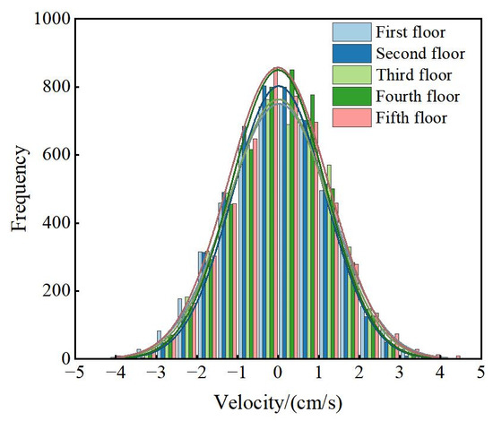
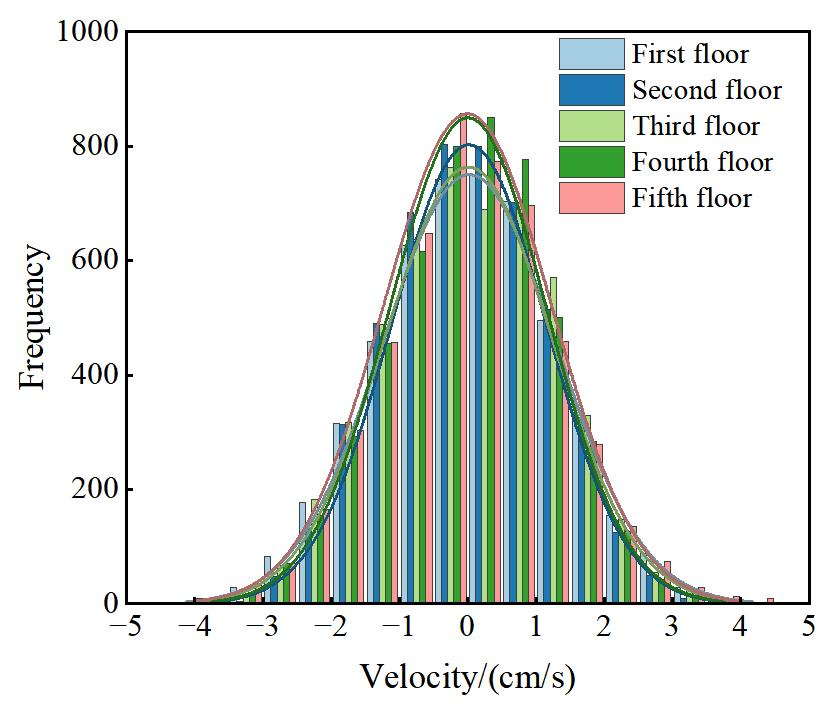
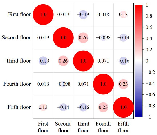
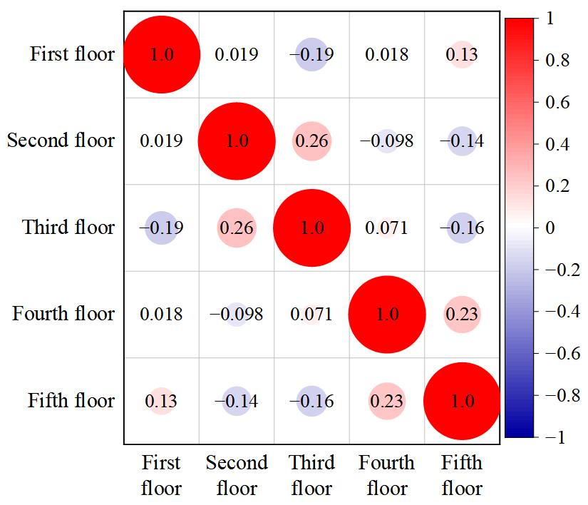
As shown in Figure 5 and Figure 6, the histograms of the velocity responses at different stories are approximately symmetric, with no evident anomalous or isolated observations. The correlation coefficients between the responses of different stories are generally low, with a maximum value below 0.3, indicating the absence of strong linear correlations among the measurement channels. This statistical analysis is used only as a preliminary quality check of the simulated responses to identify any obvious data anomalies. On this basis, the response data were subsequently employed to evaluate the feasibility and accuracy of the proposed multi-domain collaborative and clustering-fusion method for modal-parameter identification.

Figure 5. Histogram of velocity response data across different stories.

Figure 6. Correlation chart of velocity response data across different stories.

3.2. Calculation of Theoretical Value

(1)

Calculation of theoretical natural frequency

The free vibration motion equation of an n-degree-of-freedom structural system can be expressed as (Equation (19)):

$$\left[\begin{array}{cccc}{m}_1& 0& 0& 0\\ 0& m_2& 0& 0\\ 0& 0& \ddots & 0\\ 0& 0& 0& m_n\end{array}\right]\left[\begin{array}{c}{\ddot{y}}_1(t)\\ {\ddot{y}}_2(t)\\ \cdots \\ {\ddot{y}}_n(t)\end{array}\right]+\left[\begin{array}{cccc}{k}_{11}& k_{12}& \cdots & k_{1n}\\ k_{21}& k_{22}& \cdots & k_{2n}\\ ⋮& ⋮& \ddots & ⋮\\ k_{n1}& k_{n2}& \cdots & k_{\mathrm{nn}}\end{array}\right]\left[\begin{array}{c}{y}_1(t)\\ y_2(t)\\ \cdots \\ y_n(t)\end{array}\right]=\left[\begin{array}{c}0\\ 0\\ \cdots \\ 0\end{array}\right]$$

(19)

Convert it into the form of a homogeneous linear equation system:

$$M\ddot{Y}+\mathrm{KY}=0$$

(20)

where M is the mass matrix and K is the stiffness matrix.

The particular solution of this system of equations can be expressed as follows:

$$Y=\mathit{Asin} (\mathrm{wt}+\phi )$$

(21)

Substituting the particular solution into the system of equations yields

$$(K-w^{2}M)A=0$$

(22)

As we know from linear algebra, the determinant of the coefficients must be zero for the guaranteed (Equation (22)) to have a non-zero solution.

$$\left|K-w^{2}M\right|=0$$

(23)

This yields the natural frequencies of the structure, with each frequency corresponding to a specific vibration response solution.

$$Y^{(k)}=A^{(k)}\mathit{sin}(w_{k}t+{\phi }_k)$$

(24)

where w_k is the natural frequency, A^(k) is the amplitude vector, ${\phi }_k$ is the corresponding phase angle and $Y^{(k)}$ is the displacement vector, k = 1, 2, 3, …, n.

Based on the structural dynamics theory described above, the theoretical natural frequencies of the five-story frame structure are calculated. The mass matrix M and stiffness matrix K of this structure can be expressed as follows:

$$M=\left[\begin{array}{ccccc}5& 0& 0& 0& 0\\ 0& 5& 0& 0& 0\\ 0& 0& 5& 0& 0\\ 0& 0& 0& 5& 0\\ 0& 0& 0& 0& 5\end{array}\right]\times 10^5 \mathrm{kg}$$

$$K=\left[\begin{array}{ccccc}6& -3& 0& 0& 0\\ -3& 6& -3& 0& 0\\ 0& -3& 6& -3& 0\\ 0& 0& -3& 6& -3\\ 0& 0& 0& -3& 3\end{array}\right]\times 10^{5 }\mathrm{kN}/\mathrm{m}$$

The results show that the natural circular frequencies of the five-storey frame structure are 6.972 s⁻¹, 20.351 s⁻¹, 32.082 s⁻¹, 41.213 s⁻¹ and 47.005 s⁻¹, respectively. The corresponding theoretical natural frequencies are 1.1096 Hz, 3.239 Hz 5.106 Hz, 6.559 Hz and 7.481 Hz.

(2)

Calculation of the theoretical damping ratio

As stated in Rayleigh’s damping theory [36], the damping matrix is a composite of the mass and stiffness matrices; it can be expressed as (Equation (25)):

$$C=\alpha M+\beta K$$

(25)

where C is the damping matrix, α is the mass ratio damping with unit s⁻¹, and β is the stiffness ratio damping with unit s.

By left-multiplying the transposed mode shape {ϕ}_n^T and right-multiplying the mode shape {ϕ}_n in (Equation (25)), the expression becomes

$$C_n=\alpha M_n+\beta K_n$$

(26)

where C_n, M_n and K_n are the damping coefficient, mode mass, and mode stiffness of the nth-order mode, respectively. They can be expressed as follows:

$$C_n={\left\{\mathsf{\varphi }\right\}}_n^T\left[C\right]{\left\{\mathsf{\varphi }\right\}}_n$$

(27)

$$M_n={\left\{\mathsf{\varphi }\right\}}_n^T\left[M\right]{\left\{\mathsf{\varphi }\right\}}_n$$

(28)

$$K_n={\left\{\mathsf{\varphi }\right\}}_n^T\left[K\right]{\left\{\mathsf{\varphi }\right\}}_n$$

(29)

$C_n=2{\xi }_n{\omega }_n{M}_n$, ${{\omega }_n}^2=K_n/M_n$. We obtain the relationship between the damping ratio and frequency.

$${\xi }_n={\displaystyle \frac{1}{2{\omega }_n}}\alpha +{\displaystyle \frac{1}{2}}\beta {\omega }_n$$

(30)

Given the known natural frequencies, any two damping ratios ξ_n of vibration modes can be substituted into (Equation (30)) to obtain a linear equation system involving the coefficients α and β. Solving this system yields the coefficients α and β, thereby determining Rayleigh damping. Assuming the damping ratios of the ith and jth vibration modes are denoted as ξ_i and ξ_j, respectively, we derive

$${\displaystyle \frac{1}{2}}\left[\begin{array}{cc}{\displaystyle \frac{1}{{\omega }_i}}& {\omega }_i\\ {\displaystyle \frac{1}{{\omega }_j}}& {\omega }_j\end{array}\right]\left\{\begin{array}{c}\alpha \\ \beta \end{array}\right\}=\left\{\begin{array}{c}{\xi }_i\\ {\xi }_j\end{array}\right\}$$

(31)

Solving (Equation (31)) yields

$$\alpha ={\displaystyle \frac{2{\omega }_i{\omega }_j({\xi }_i{\omega }_j-{\xi }_j{\omega }_i)}{{{\omega }_j}^2-{{\omega }_i}^2}}$$

(32)

$$\beta ={\displaystyle \frac{2({\xi }_j{\omega }_j-{\xi }_i{\omega }_i)}{{{\omega }_j}^2-{{\omega }_i}^2}}$$

(33)

According to the Rayleigh damping theory, the damping ratios corresponding to the first two natural frequencies are ξ₁ = ξ₂ = 0.01. By combining ω₁ = 6.972 s⁻¹ and ω₂ = 20.351 s⁻¹, the proportional coefficients of the damping matrix can be calculated as α = 0.1039 s⁻¹ and β = 7.3199 × 10⁻⁴ s.

Given the proportional coefficients α and β of the damping matrix, substituting ω₃ = 32.082 s⁻¹, ω₄ = 41.213 s⁻¹ and ω₅ = 47.005 s⁻¹ into (Equation (30)) yields the corresponding ξ₃ = 0.0134, ξ₄ = 0.0163, and ξ₅ = 0.0183. The damping matrix can be expressed as follows:

$$C=\alpha M+\beta K=\left[\begin{array}{ccccc}4.9112& -2.196& 0& 0& 0\\ -2.196& 4.9112& -2.196& 0& 0\\ 0& -2.196& 4.9112& -2.196& 0\\ 0& 0& -2.196& 4.9112& -2.196\\ 0& 0& 0& -2.196& 2.7152\end{array}\right]\times 10^5 \mathrm{N}\cdot \mathrm{s}/\mathrm{m}$$

3.3. Analysis of Identification Results from Different Methods

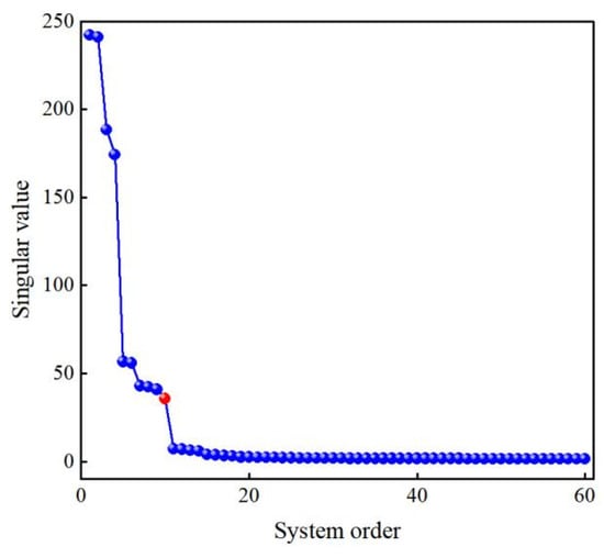
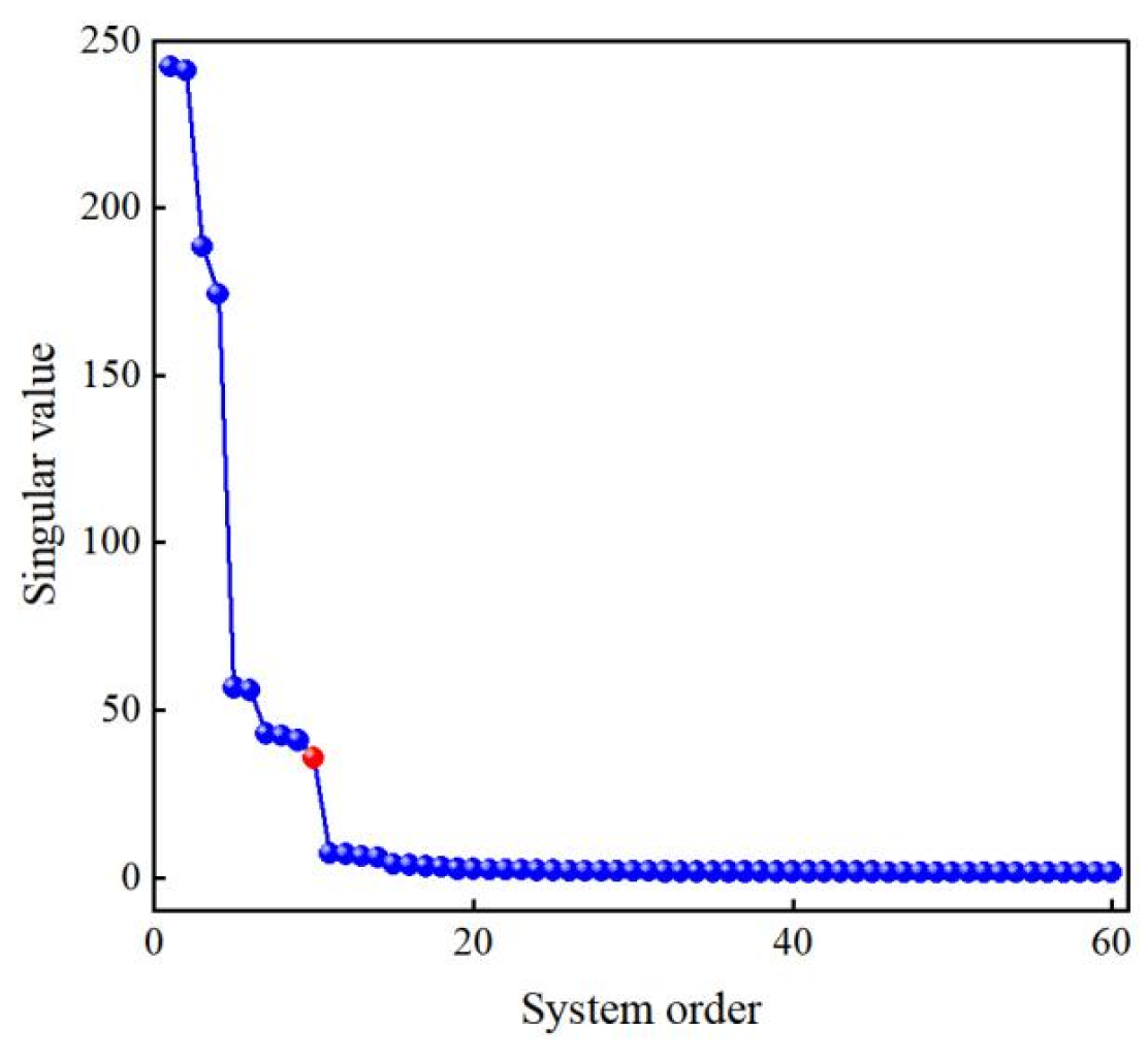
Using the second random white noise excitation as an example, the SSI-cov method was employed to identify the natural frequencies and damping ratios of the structure. This method constructs covariance response data by collecting vibration velocities from five distinct measurement points. The length l of the velocity data for each measurement point is 1000 Hz ×5 s = 5000. The system order was determined using the singular value jumping method, as illustrated in Figure 7. Figure 7 reveals that singular values no longer exhibit significant jumps after the 10^th order, indicating that the state matrix order is 10 and the system order is 5. The numerical model order M is 5. When the stable graph order H = 4M, the identification results are relatively optimal [37]. The number of rows i in a Toeplitz matrix is related to the sampling frequency f_s and the structural fundamental frequency f₀, where i = (1~2) × f_s/2f₀. The stable graph order and Toeplitz matrix row count are set to 20 and 500, respectively, with 5 channels.

Figure 7. SSI-cov method singular value.

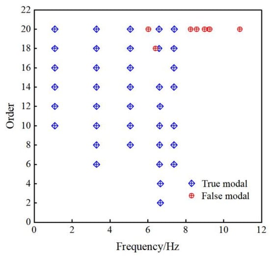
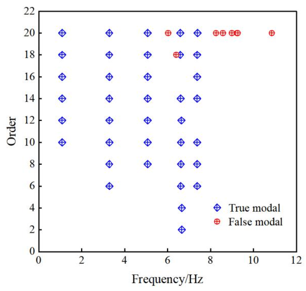
To select stable poles and natural frequency orders, the frequency error and damping ratio tolerance are set at 1% and 5%, respectively, enabling automatic identification of structural natural frequencies and damping ratios. The modal parameter identification stability diagram is shown in Figure 8. The process exhibits minimal false poles with more continuous stable axes. The identification results of the SSI-cov method for structural natural frequencies and damping ratios are presented in Table 1.

Figure 8. Stability diagram of dynamic characteristic identification.

Table 1. Natural frequency and damping ratio of the identification framework structure for SSI-cov method.

Order	Natural Frequency/Hz	Damping Ratio/%
1	1.0899	1.042
2	3.2828	0.9731
3	5.0642	1.2841
4	6.5846	1.5694
5	7.3996	1.9027

The power spectral densities of the response signals were estimated using Welch’s method. Each response record was divided into overlapping segments using a 2000-point Hamming window with 50% overlap, and the FFT length was set to 16,384 points, corresponding to a frequency-grid spacing of 0.0610 Hz.

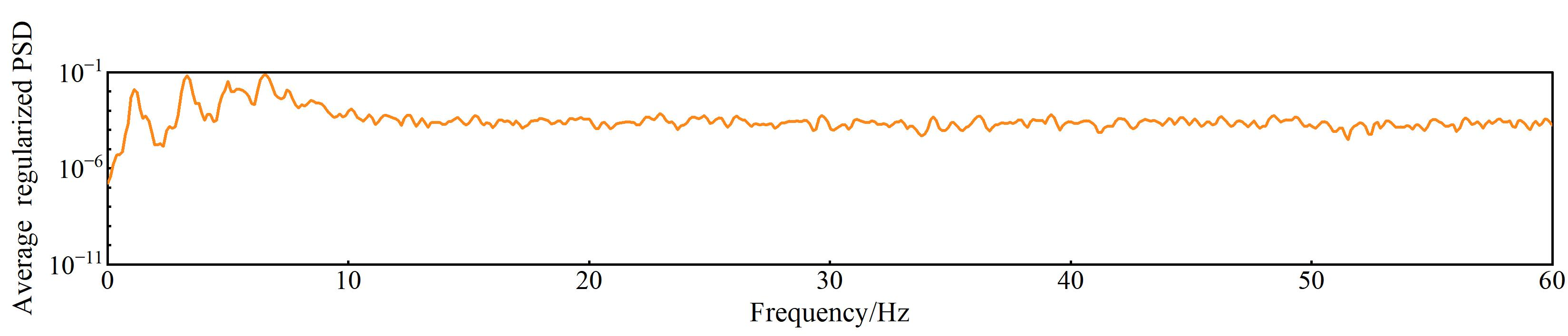
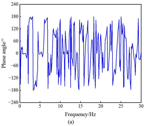
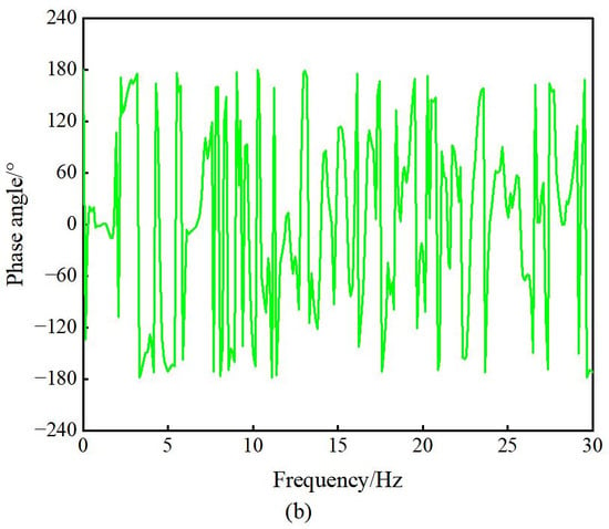
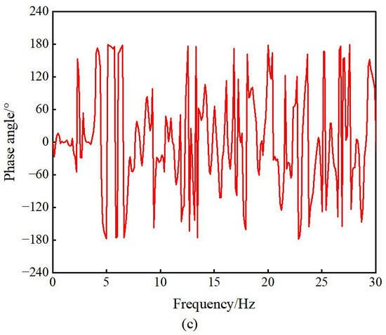
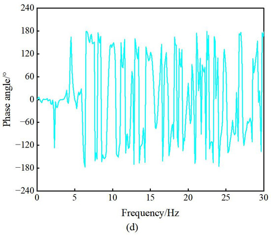
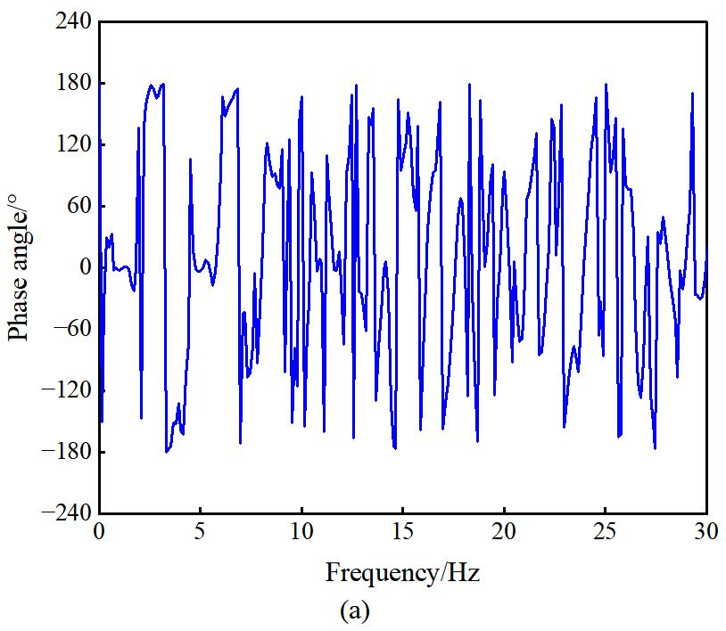
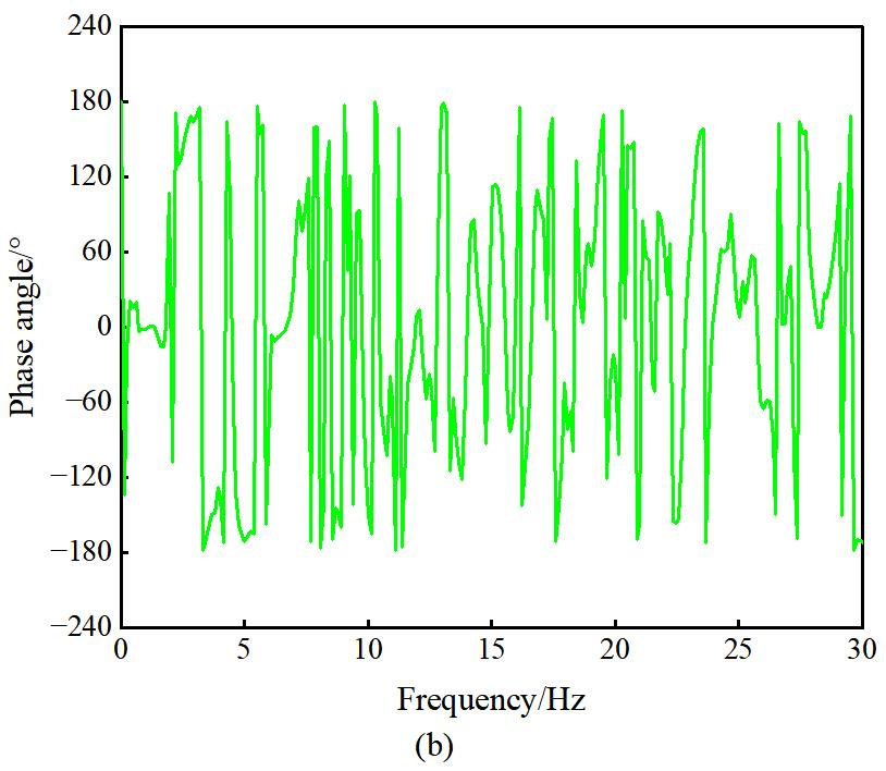
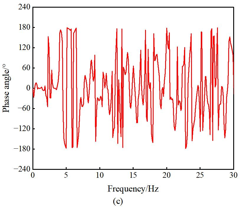
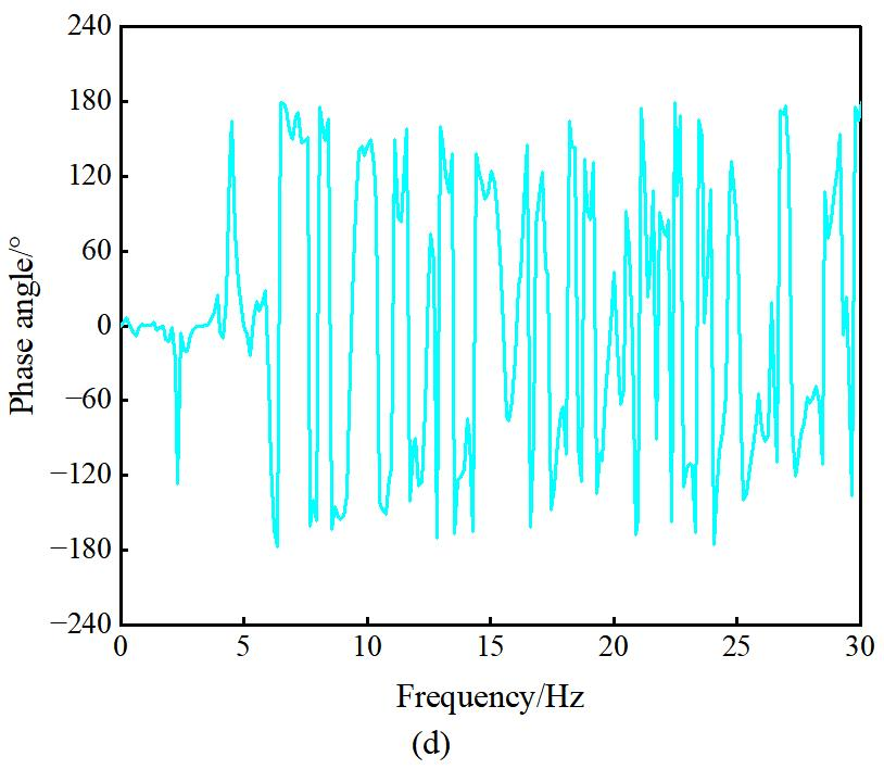
The power spectra of different measurement points in the numerical model are shown in Figure 9. The self-power spectra from various measurement points were synthesized into an average normalized power spectrum, and the damping ratio was calculated using the RDT method. Considering the short-duration and non-stationary characteristics of blasting-induced vibration signals, the parameters for modal damping estimation using the RDT were selected based on the temporal characteristics of the response signals. The triggering threshold was set to 0.5 times the standard deviation of the response signal, and the segment length was set to 2000 samples (2 s). A total of 60–114 valid triggered segments were obtained for the candidate modes. These segments were ensemble-averaged to extract the random decrement signatures, from which the modal damping ratios were subsequently estimated. The average normalized power spectra of different measurement points in the numerical model are illustrated in Figure 10. As shown in Figure 10, the frequencies corresponding to the peak points of the average normalized power spectrum are 1.0986 Hz, 3.2959 Hz, 5.0049 Hz, 6.4697 Hz, and 7.4463 Hz, respectively. The phase-frequency curves between different target points and the reference point are presented in Figure 11, with the corresponding phase angles at different frequencies listed in Table 2. According to Table 2, the phase angles of the target points at 1.0986 Hz, 3.2959 Hz, 5.0049 Hz, and 6.4697 Hz are all close to 0° or ±180° (allowing ±30° fluctuation), indicating that these four frequencies are natural frequencies of the structure. The phase angles at 7.4463 Hz for the target points are −102.25°, 93.787°, −53.749°, and 147.64°, which do not approach 0° or ±180°. For sufficiently separated modes, phase values close to 0° or ±180° may serve as an auxiliary indicator for modal identification. Nevertheless, the use of a fixed phase threshold is subject to certain limitations, as the phase response can be influenced by measurement-point locations and noise contamination. Consequently, candidate modes should not be rejected solely on the basis of a fixed phase threshold; rather, the phase information should be incorporated as a supplementary criterion in the overall assessment. The spectral peak at 7.4463 Hz is therefore retained, given its small deviation from the fifth theoretical natural frequency of 7.4811 Hz.

Figure 9. Power spectrum of different measurement points in the numerical model. (a) Target point 1. (b) Target point 2. (c) Target point 3. (d) Target point 4. (e) Reference point 5.

Figure 10. Average normalized power spectrum at different measurement points of the numerical model.

Figure 11. Phase-frequency curves between different target points and reference points. (a) Target point 1. (b) Target point 2. (c) Target point 3. (d) Target point 4.

Table 2. Phase angle of the identification framework structure for PP method.

Peak Frequency/Hz	Phase Angle/°
	Target Point 1	Target Point 2	Target Point 3	Target Point 4
1.0986	−0.5787	−0.36571	0.23647	0.31957
3.2959	−179.68	−178.01	−0.065515	−0.33988
5.0049	−3.8547	−171.45	−177.46	−0.36573
6.4697	162.01	−6.232	177.72	178.59
7.4463	−102.25	93.787	−53.749	147.64

Based on the modal parameter identification results through the SSI-cov and PP method, combined with automatic classification using the K-means clustering algorithm, the first five natural frequencies and damping ratios of the shear frame structure numerical model were determined and compared with theoretical values. Fifteen sets of natural frequency and damping ratio data were clustered using the K-means algorithm, with the clustering centers of different categories serving as identification values for natural frequencies and damping ratios in multi-domain collaborative and clustering fusion.

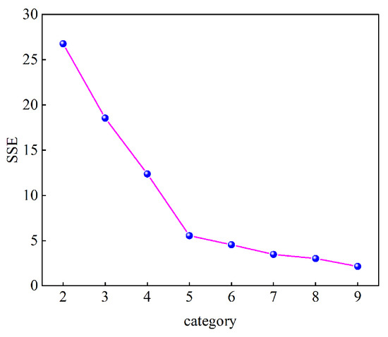
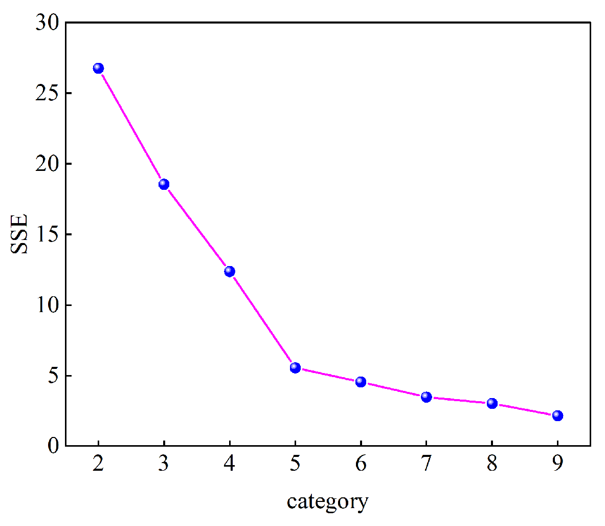
The K-means algorithm was initialized with different centroid configurations, and the clustering procedure was repeated 100 times. The solution with the minimum within-cluster sum of squares was retained as the final clustering result. A fixed random seed was used throughout the analysis to ensure reproducibility. Prior to clustering, the natural-frequency and damping ratio features were standardized using z-score normalization [38] to eliminate the effects of different physical dimensions and numerical scales. Manhattan distances [39] were then calculated in the standardized feature space. The variation in the sum of squared errors (SSE) with the number of clusters is shown in Figure 12. The SSE decreases progressively as the number of clusters increases. A pronounced reduction is observed as the number of clusters increases from 2 to 5, whereas the rate of decrease becomes substantially smaller for K > 5, resulting in a distinct elbow at K = 5. Therefore, the number of clusters for the natural-frequency and damping ratio data of the numerical model was set to 5.

Figure 12. The variation in the SSE with the number of clusters.

The clustering results of natural frequencies and damping ratios are shown in Table 3. The clustering categories of natural frequencies and damping ratios are 5, with clustering centers for natural frequencies being 1.1067, 3.2549, 5.1324, 6.5722, and 7.4539, and clustering centers for damping ratios being 0.98, 1.01, 1.33, 1.59, and 1.79.

Table 3. The clustering results of natural frequencies and damping ratios.

Order	Natural Frequency/Hz			Damping Ratio/%
	Cluster Center	Maximum Value	Minimum Value	Cluster Center	Maximum Value	Minimum Value
1	1.1067	1.1267	1.0899	0.98	0.99	0.95
2	3.2549	3.418	3.1598	1.01	1.04	1.01
3	5.1324	5.4723	5.0049	1.33	1.4	1.22
4	6.5722	6.8359	6.3477	1.59	1.63	1.52
5	7.4539	7.8125	7.2116	1.79	1.94	1.74

The identification results of natural frequencies and damping ratios for the frame structure are presented in Table 4 and Table 5, respectively. The PP-K-means method failed to identify the fifth-order natural frequency and damping ratio, while the identification errors for the first four orders were less than 2% and 8%, with maximum errors of 1.98% and 7%, respectively. Compared to the theoretical values from the numerical model, the SSI-cov-K-means method demonstrated superior performance, achieving maximum identification errors of 1.78% and 4.2% for the first five orders. When comparing the SSI-cov-K-means method with the PP-K-means method, the MDCCF approach produced identification results that closely matched the theoretical values, with errors below 1% and 3% for natural frequencies and damping ratios, respectively, and maximum errors of 0.52% and 2.45%. These findings indicate that the proposed method effectively identifies structural modal parameters with high accuracy and practical applicability.

Table 4. Comparison of natural frequency identification results for frame structures.

Order	Theoretical Natural Frequency/Hz	Identification Results/Hz			Error/%
		SSI-cov-K-Means	PP-K-Means	MDCCF	SSI-cov-K-Means	PP-K-Means	MDCCF
1	1.1096	1.0899	1.0986	1.1067	1.78	0.99	0.26
2	3.239	3.2828	3.2959	3.2549	1.35	1.76	0.49
3	5.1059	5.0642	5.0049	5.1324	0.82	1.98	0.52
4	6.5592	6.5846	6.4697	6.5722	0.39	1.36	0.21
5	7.4811	7.3996		7.4539	1.09		0.36

Table 5. Comparison of identification results for the damping ratio of the frame structure.

Order	Theoretical Damping Ratio/%	Identification Results/%			Error/%
		SSI-cov-K-Means	PP-K-Means	MDCCF	SSI-cov-K-Means	PP-K-Means	MDCCF
1	1	1.042	1.07	0.98	4.2	7	2
2	1	0.9731	0.96	1.01	2.69	4	1
3	1.34	1.2841	1.36	1.33	4.17	1.49	0.75
4	1.63	1.5694	1.58	1.59	3.72	3.07	2.45
5	1.83	1.9027		1.79	3.97		2.19

3.4. Statistical Evaluation of Identification Robustness

To evaluate the stability and robustness of different identification methods under noisy conditions, 15 independent Monte Carlo simulations were conducted for each signal-to-noise ratio (SNR) level, and the corresponding mean values and standard deviations were calculated. Zero-mean Gaussian white noise was adopted in the simulations, and all noisy cases were generated by superimposing random noise on the same original response data. The PCA-K-means method was implemented based on the procedure reported in Ref. [40], in which PCA was employed to reduce the dimensionality of the candidate modal features, and the first principal component was selected as the input to K-means clustering for modal screening and identification. No additional artificial measurement noise was introduced beyond the prescribed noise levels.

A statistical comparison of the natural frequency identification errors under different SNRs is shown in Table 6. A statistical comparison of the damping ratio identification errors under different signal-to-noise ratios is shown in Table 7. As shown in Table 6 and Table 7, although the identification performance of all methods deteriorates as the noise level increases, MDCCF consistently exhibits lower mean errors and smaller standard deviations than PCA-K-means, SSI-COV-K-means and PP-K-means. These results demonstrate the comparatively stronger noise robustness and statistical stability of the proposed fusion framework over the investigated SNR range.

Table 6. Statistical comparison of the natural frequency identification errors under different signal-to-noise ratios.

SNR/dB	PCA-K-Means [40]/%	SSI-cov-K-Means/%	PP-K-Means/%	MDCCF/%
30	1.05 ± 0.33	1.16 ± 0.15	1.78 ± 0.42	0.39 ± 0.31
20	1.61 ± 0.59	1.28 ± 0.46	1.84 ± 0.74	0.45 ± 0.21
10	2.74 ± 0.96	2.31 ± 0.82	2.09 ± 0.77	0.93 ± 0.38

Table 7. Statistical comparison of the damping ratio identification errors under different signal-to-noise ratios.

SNR/dB	PCA-K-Means [40]/%	SSI-cov-K-Means/%	PP-K-Means%	MDCCF/%
30	4.02 ± 1.18	3.84 ± 1.46	3.96 ± 0.98	1.94 ± 0.72
20	5.07 ± 1.52	4.01 ± 1.26	4.22 ± 1.24	2.00 ± 0.68
10	7.26 ± 2.20	6.14 ± 1.98	5.47 ± 1.76	3.46 ± 1.15

4. Identification of Modal Parameters for Brick-Concrete Structures Subjected to Open-Pit Deep-Hole Blasting

4.1. Description of the Brick-Concrete Structure Building

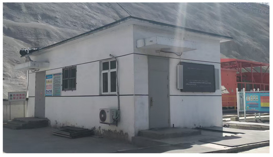
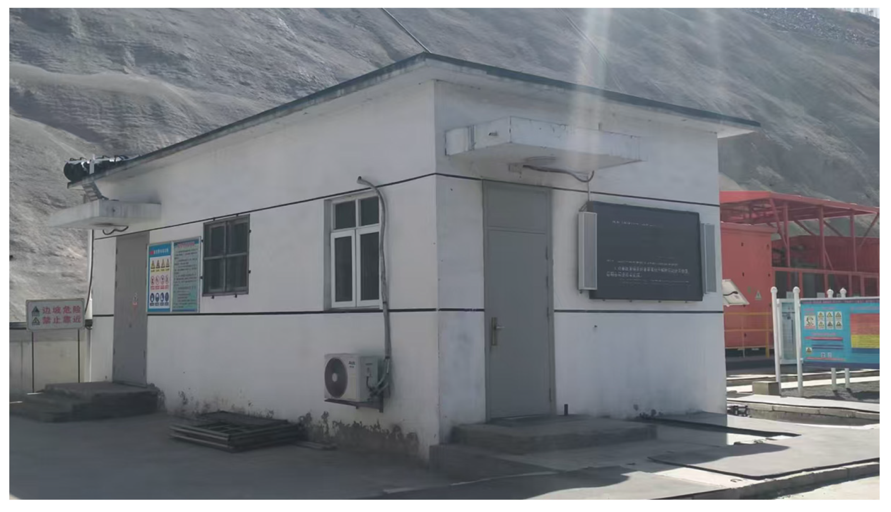
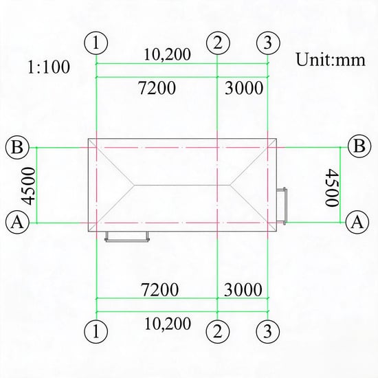
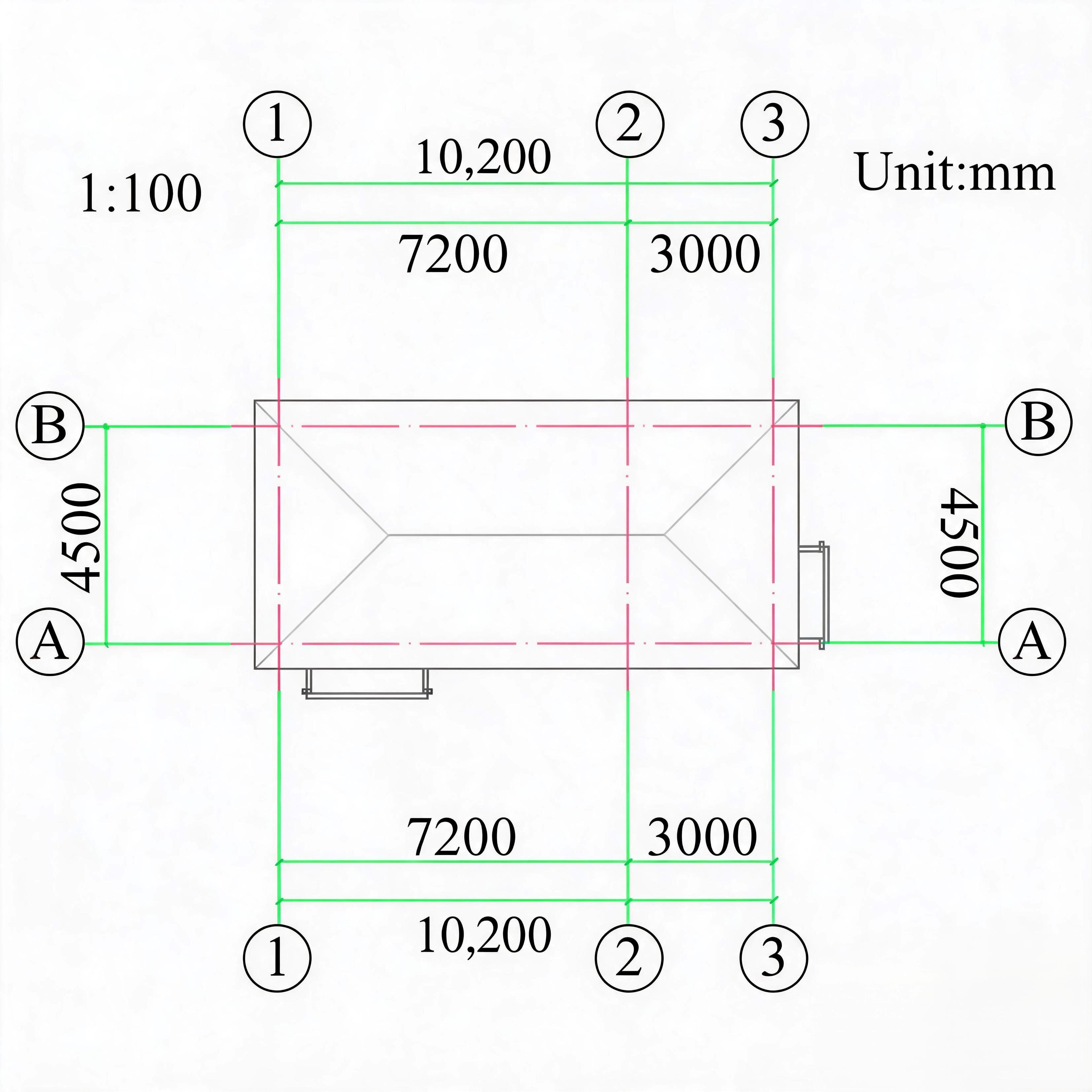
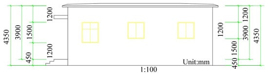
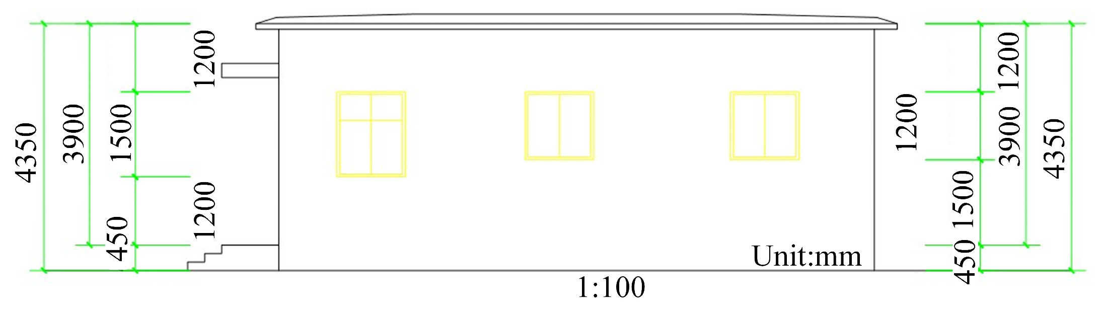
The case-study building is a single-story brick masonry structure with a total story area of 49.49 m². The load-bearing walls are constructed using MU10 fired shale perforated bricks with M7.5 masonry mortar. The tie columns, ring beams, reinforced-concrete roof slab, and other reinforced-concrete components are constructed using C25-grade concrete. The building measures 10.44 m in the east–west direction and 4.74 m in the north–south direction, with an overall height of 4.35 m.

The foundation has a cross-sectional dimension of 500 mm × 350 mm, while the beams and tie columns have cross-sectional dimensions of 240 mm × 450 mm and 240 mm × 240 mm, respectively. Both the interior and exterior load-bearing walls are 240 mm thick, and the reinforced-concrete roof slab has a thickness of 100 mm. An exterior view of the case-study building is shown in Figure 13. A plan view of the brick-concrete building is shown in Figure 14. An elevation view of the brick-concrete building is shown in Figure 15.

Figure 13. Exterior view of the case-study building.

Figure 14. Plan view of the brick-concrete building.

Figure 15. Elevation view of the brick-concrete building.

4.2. Experimental Instruments

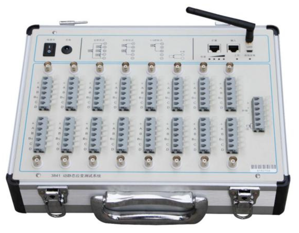
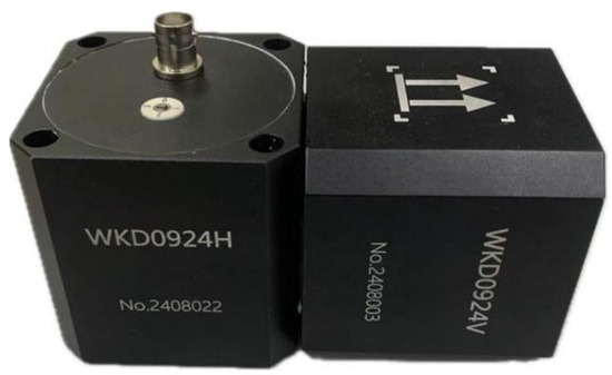
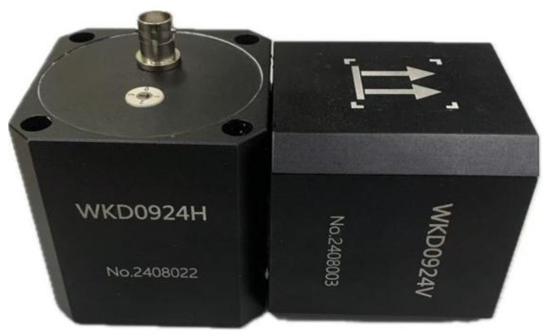
The field experiment primarily utilized the WKD3841 dynamic–static signal testing system and the WKD0924V/H magnetoelectric velocity sensor to collect blasting vibration signals from brick-concrete structures, employing the MDCCF method to identify modal parameters. The WKD3841 system and the WKD0924V/H magnetoelectric velocity sensor, manufactured by Tianjin Weikende Measurement & Control Equipment Technology Co., Ltd., (Tianjin, China) is a high-performance testing solution supporting dynamic strain, voltage, and integrated electronics piezo-electric (IEPE) measurements. It enables simultaneous data acquisition from multiple points, making it ideal for engineering scenarios with dispersed measurement points. Figure 16 shows the WKD3841 system, while its technical specifications are detailed in Table 8.

Figure 16. WKD3841 static and dynamic signal testing system.

Table 8. Parameters of WKD3841 dynamic and static signal testing system.

Parameter	Description
Number of channels	16
Sample mode	Each channel independently and synchronously acquires data in parallel
IEPE supply electricity	+24 V/4 mA
Analog to digital digit capacity	24 bits
Communication mode	Multi-unit networking
Supply bridge voltage	2 Vdc

The WKD0924V/H magnetoelectric velocity sensor is a versatile instrument utilizing electromagnetic induction principles for ultra-low frequency (ULF) or low-frequency vibration measurement. It is primarily designed for pulsation measurement of ground and building structures, industrial vibration measurement of general structures, ULF amplitude measurement of highly flexible structures, and weak vibration detection. As shown in Figure 17, the technical specifications of the WKD0924V/H magnetoelectric velocity sensor are detailed in Table 9.

Figure 17. Electromagnetic velocity sensor.

Table 9. Technical specifications of electromagnetic velocity sensors.

Gear	Measurement Mode	Sensitivity	Frequency Response Range/Hz	Maximum Measurement Range	Temperature/(°C)
0	Acceleration	~0.3 V/(m/s2)	0.25~100	20 m/s2	−10~+50
1	Low velocity	~20 V/(m/s)	1~100	0.12 m/s
2	Medium velocity	~4.8 V/(m/s)	0.5~100	0.3 m/s
3	High velocity	~0.35 V/(m/s)	0.17~100	0.6 m/s

4.3. Experimental Design

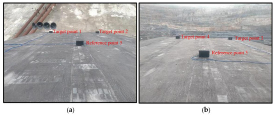
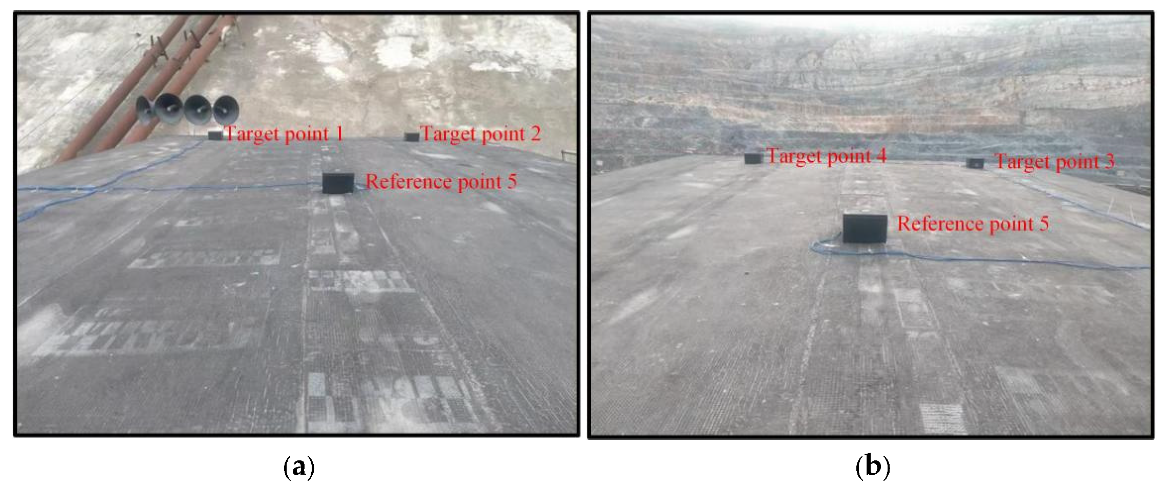
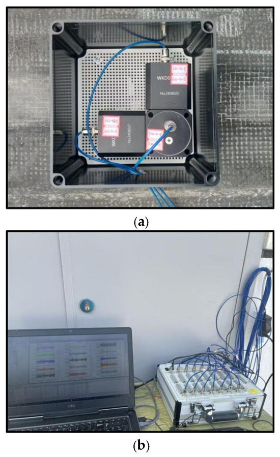
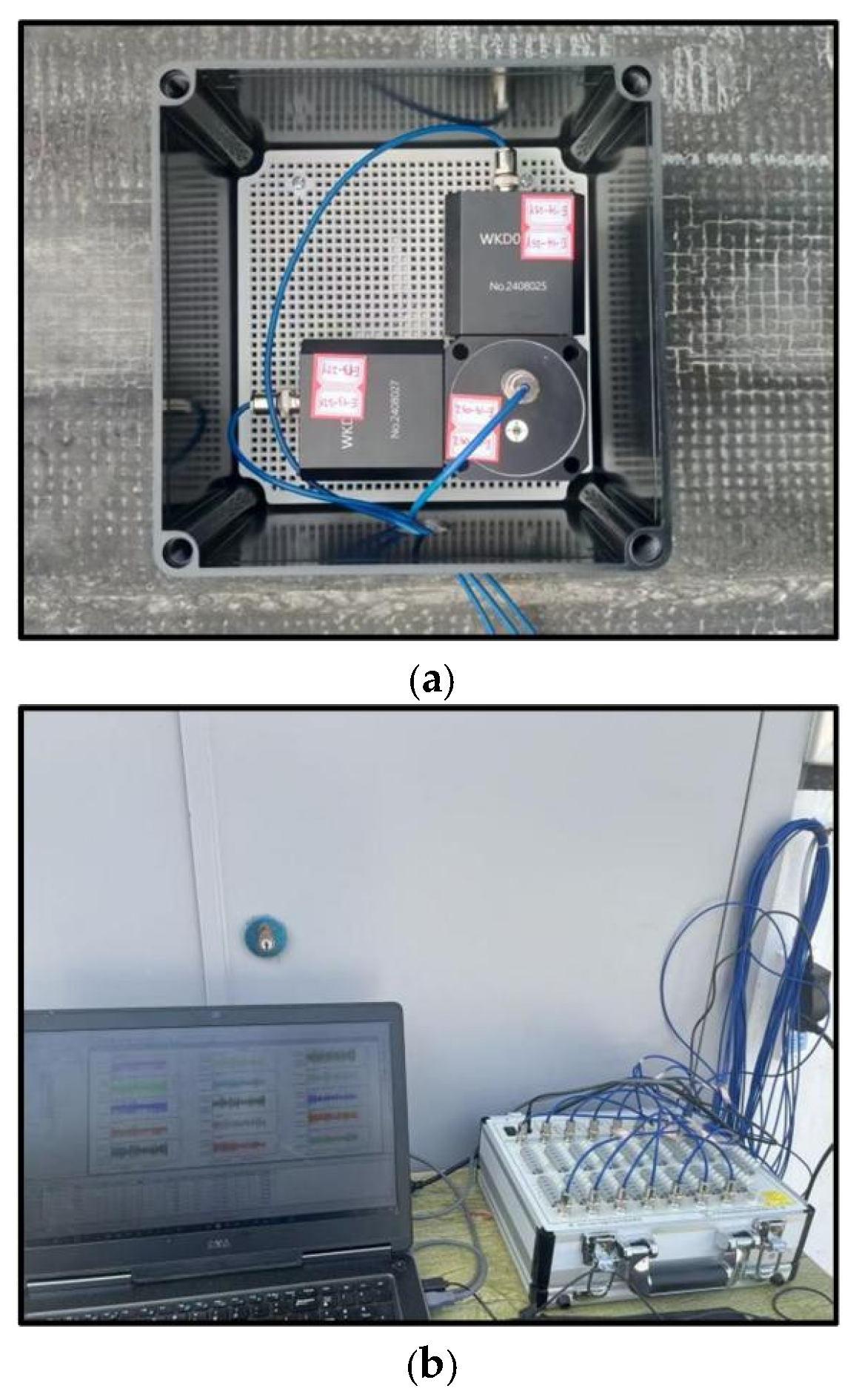
Five measurement points are installed on the roof of a brick-concrete structure building, each equipped with two WKD0924V and one WKD0924H magnetoelectric velocity sensors. The WKD0924V and WKD0924H sensors are used to collect blasting vibration signals in the horizontal (tangential and radial) and vertical directions, respectively. The magnetoelectric sensors are connected to the WKD3841 dynamic–static signal testing system via custom cables, and the measured blasting vibration signals are stored in a computer. The monitoring point layout is shown in Figure 18, and the field experiment monitoring instruments are shown in Figure 19.

Figure 18. Layout of monitoring points. (a) Position 1. (b) Position 2.

Figure 19. Field experiment monitoring instrument. (a) Three-directional magnetoelectric velocity sensor. (b) Computer and WKD dynamic and static signal testing system.

4.4. Identification of Natural Frequency and Damping Ratio of Brick-Concrete Structure Buildings

The WKD3841 dynamic–static signal testing and analysis system, along with the WKD0924V and WKD0924H magnetoelectric velocity sensors, was employed to monitor the vertical and horizontal (tangential and radial) blast-induced vibrations in brick-concrete structures. With a sampling frequency of 1000 Hz and continuous recording, 25 mine production blast vibrations were detected. For the 25 production blasts conducted at the mine, the blast distances ranged from 214 to 845 m, and the maximum charge weight per delay ranged from 250 to 850 kg. The inter-row delay time was 100 ms for all blasts, while the inter-hole delay time was 42 ms. The scaled distance ranged from 22.59 to 134.14 m/kg^1/3. According to the Sadowski empirical equation, the scaled distance is defined as follows:

$$Z={\displaystyle \frac{\mathrm{R}}{Q^{1/3}}}$$

(34)

where Z is the scaled distance (m/kg^1/3), R is the blasting distance (m), and Q is the maximum charge weight per delay (kg).

Taking the third blast-induced seismic wave recorded at a vertical measurement point as an example, modal parameter identification for brick-concrete structures was performed using the PP and SSI-cov method. The same procedure was applied to identify modal parameters in the horizontal (tangential and radial) directions and is not repeated here.

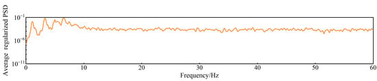
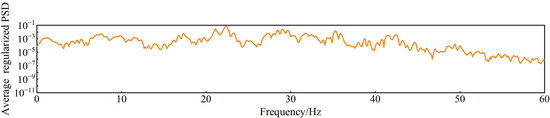
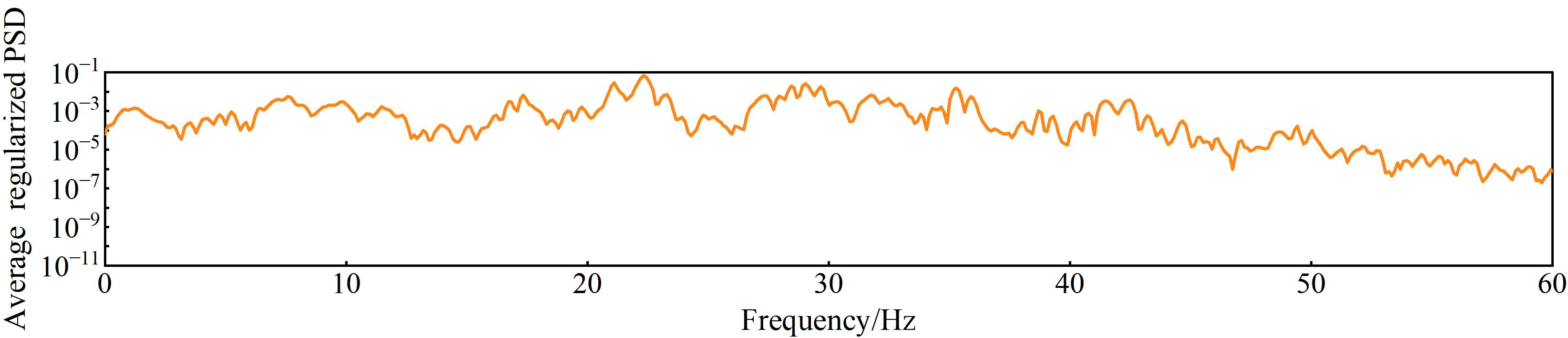
The field-measured signal was sampled at 1000 Hz with a record duration of 11.019 s. Spectral estimation was performed using a 2000-point Hamming window with 50% overlap, and each segment was zero-padded to 16,384 points for FFT computation, resulting in a frequency-grid spacing of 0.0610 Hz. The effective frequency resolution was characterized by the −3 dB main-lobe width of the Hamming window; for the 2 s analysis window, the corresponding resolution was approximately 0.65 Hz. Figure 20 presents the average normalized power spectra of brick-concrete structures across different measurement points, with the corresponding peak frequencies and phase angles listed in Table 10. The spectrum reveals peak frequencies in descending order: 7.5684 Hz, 17.334 Hz, 21.1182 Hz, 22.3389 Hz, 28.4424 Hz, 29.0527 Hz, 29.6631 Hz, 35.2783 Hz, 41.5039 Hz, and 42.4805 Hz.

Figure 20. Average normalized power spectrum at different measurement points of the brick-concrete structure building.

Table 10. Phase angle corresponding to different peak frequencies.

Peak Frequency/Hz	Phase Angle/°
	Target Point 1	Target Point 2	Target Point 3	Target Point 4
7.5684	−10.555	−9.7697	14.073	11.628
17.334	−37.083	51.41	−33.684	115.79
21.1182	15.092	−24.722	56.001	−37.781
22.3389	−6.889	9.787	−145.09	−142.03
28.4424	110.54	−176.68	−112.77	−111
29.0527	97.821	−173	−122.39	−110.83
29.6631	140.88	−120.75	−106.55	−120.35
35.2783	48.279	95.467	15.99	−84.205
41.5039	−143.1	−124.45	21.848	−50.899
42.4805	−140.1	−82.261	−22.252	−88.078

As shown in Table 10, the phase angles corresponding to the peak frequencies of 7.5684 Hz are all close to 0° or ±180° (allowing ±30° fluctuations), indicating that 7.5684 Hz can be considered the candidate mode of brick-concrete structures. The phase responses at 17.334 Hz and 29.6631 Hz show no phase angles close to 0° nor ±180°. By comparison, at minimum, one measurement point exhibits the expected phase characteristic at 28.4424 Hz, 29.0527 Hz, 35.2783 Hz, 41.5039 Hz, and 42.4805 Hz, while two measurement points show such consistency at 21.1182 Hz and 22.3389 Hz. These frequencies are therefore retained as candidate modes for further evaluation, whereas 17.334 Hz and 29.6631 Hz receive no supporting evidence from the phase information.

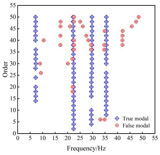
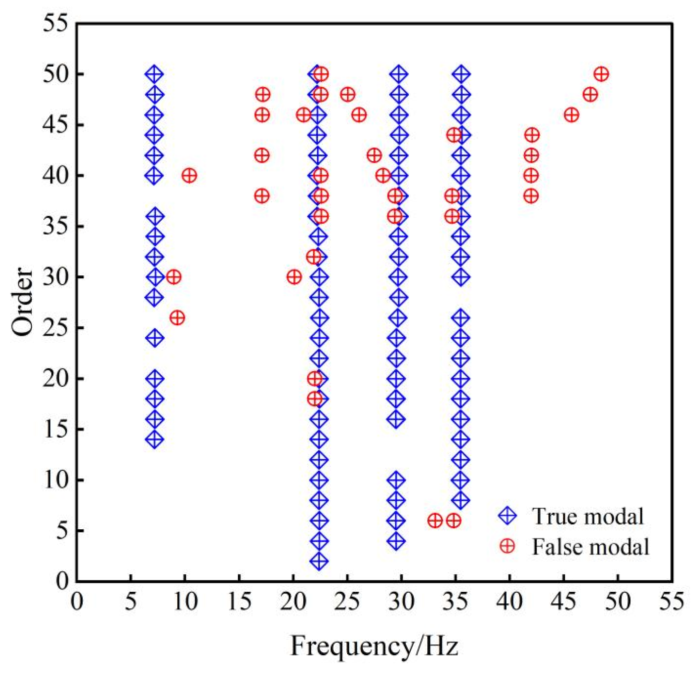
The SSI-cov method was employed to identify modal parameters of brick-concrete structures. The model was configured with a minimum order of 6 and a maximum order of 50, a Toeplitz matrix with 250 rows, and 5 channels. Frequency error and damping ratio error were set at 1% and 5%, respectively. The stability diagram of modal parameter identification using the SSI-cov method is shown in Figure 21. The SSI-cov method primarily identified four distinct real modal frequencies, concentrated around 7.152 Hz, 22.2088 Hz, 29.7453 Hz, and 35.5245 Hz. The stable axes formed by these real modal frequencies exhibited a relatively continuous distribution, indicating good consistency in modal parameters across different orders. In contrast, false modal frequencies displayed isolated or discrete distributions, lacking cross-order stability and demonstrating relatively poor performance.

Figure 21. Stability diagram of modal identification for the brick-concrete structure building using the SSI-cov method.

This study employs the K-means algorithm to cluster the natural frequencies and damping ratios identified by the SSI-COV and PP methods from 25 blasting events, the cluster centers of the different groups are taken as the identified modal parameters in the proposed multi-domain collaborative and clustering fusion method. The clustering results of natural frequencies and damping ratios are presented in Table 11. The number of clusters was determined using the SSE criterion, resulting in a total of 10 clusters. The cluster centers for natural frequencies are 7.69 Hz, 10.559 Hz, 17.2068 Hz, 22.095 Hz, 27.099 Hz, 29.7741 Hz, 34.668 Hz, 40.039 Hz, 48.7882 Hz, and 50.6476 Hz, while the cluster centers for damping ratios are 4.4602%, 3.705%, 2.8618%, 2.4161%, 1.9%, 1.45%, 1.11%, 0.8579%, 0.59%, and 0.3493%.

Table 11. Identification of the natural frequency and damping ratio of brick-concrete structures using the MDCCF method.

Order	Natural Frequency/Hz			Damping Ratio/%
	Cluster Center	Minimum Value	Maximum Value	Cluster Center	Minimum Value	Maximum Value
1	7.69	5.737	9.6436	4.4602	4.07	4.93
2	10.559	9.765	13.062	3.705	3.28	4.0451
3	17.2068	14.648	19.165	2.8618	2.67	3.22
4	22.095	19.775	24.4738	2.4161	2.2072	2.6509
5	27.099	24.6478	28.5061	1.9	1.73	2.1742
6	29.7741	28.7042	31.738	1.45	1.2953	1.7
7	34.668	32.8015	37.354	1.11	0.9818	1.29
8	40.039	38.1876	41.9503	0.8579	0.72	0.97
9	48.7882	46.875	49.987	0.59	0.4678	0.7127
10	50.6476	50.171	53.7765	0.3493	0.1209	0.4503

5. Discussion

Due to the non-homogeneity of materials, structural complexity, the transient and high-energy nature of blasting vibration signals, and uncertainties such as identification method errors, the natural frequency and damping ratio of brick-concrete structures are not fixed values but typically exhibit a degree of uncertainty. Relying solely on a single method for modal identification often results in significant errors. By adopting a framework integrating data evaluation, multi-domain identification, and clustering fusion, this study employs an MDCCF method for modal parameter identification. Compared to traditional methods, this approach addresses limitations such as high identification errors and poor adaptability in single-method systems, thereby improving accuracy under complex environmental excitations like blasting vibration. This methodology enhances the reliability and robustness of identifying modal parameters in brick-concrete structures subjected to blasting vibrations, yielding more accurate natural frequency and damping ratio measurements. To further validate the proposed method’s effectiveness, this paper conducts a probabilistic distribution analysis of the identification results.

5.1. Relationship Between the First-Mode Natural Frequency and PPV

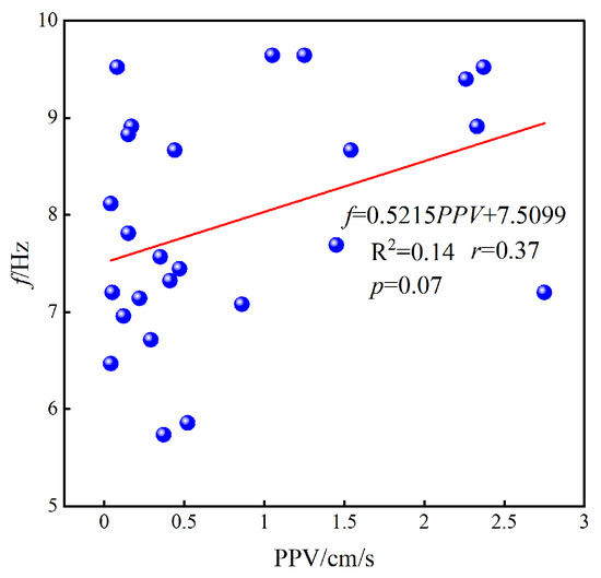
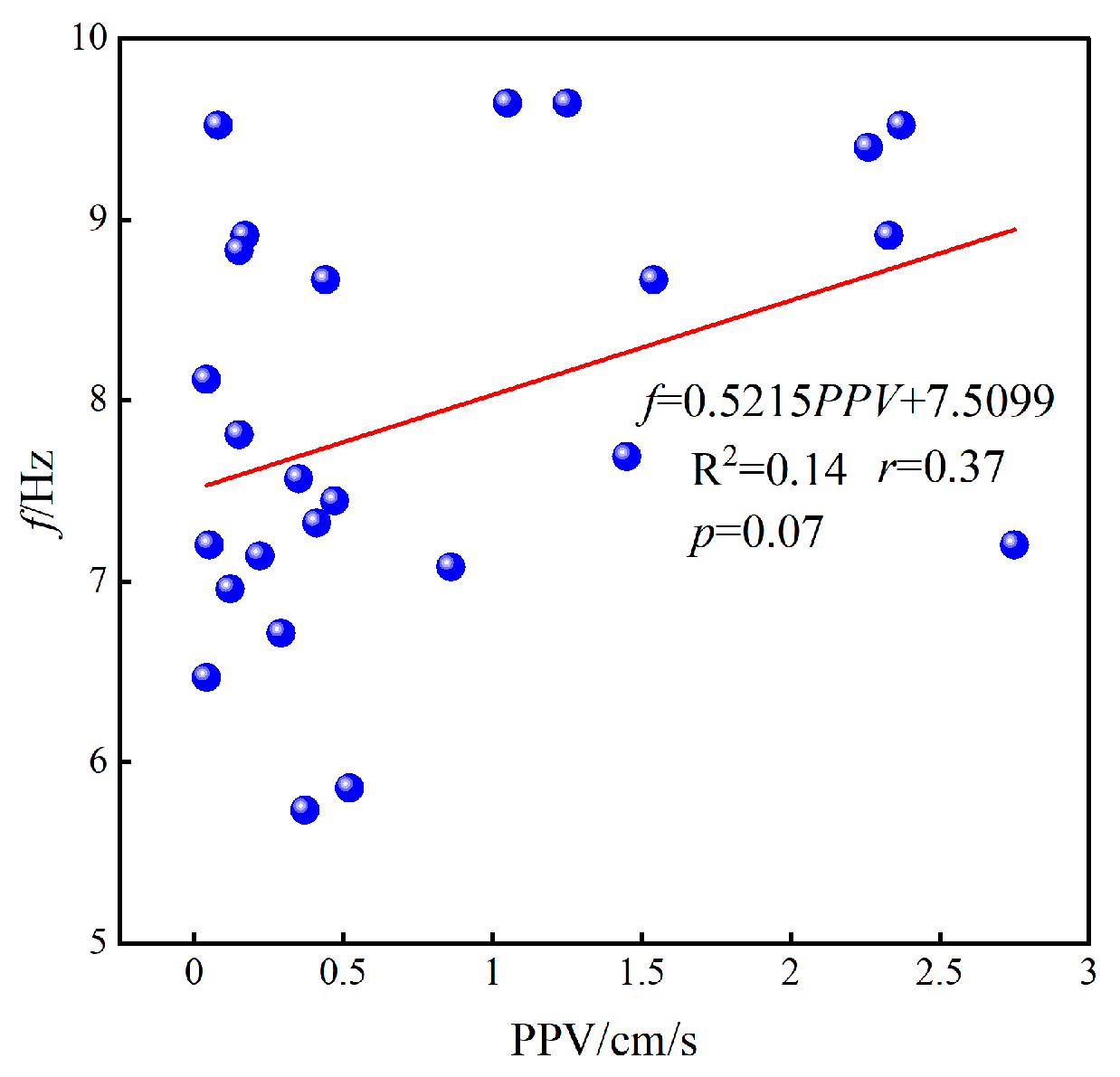
To examine whether the variability in the identified natural frequencies is associated with the vibration amplitude, the first-mode natural frequency (f) identified from each blasting event was compared with the corresponding peak particle velocity (PPV), as shown in Figure 22. As shown in Figure 22, the Pearson correlation coefficient (r) is 0.37, and the coefficient of determination (R²) is 0.14. The fitted slope is positive rather than negative, and no systematic decrease in the first-mode natural frequency with increasing PPV is observed. Therefore, within the vibration-amplitude range considered in this study, the experimental results do not show an evident amplitude-dependent frequency-softening trend. Accordingly, the variability of the identified natural frequencies is subsequently characterized from a statistical perspective.

Figure 22. Relationship between the order frequency and PPV for different blasting events.

5.2. Time-Frequency Characteristics of the Blast-Induced Structural Response

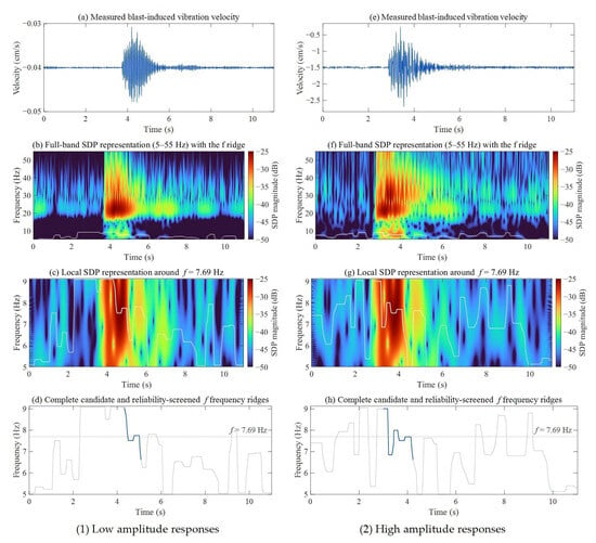
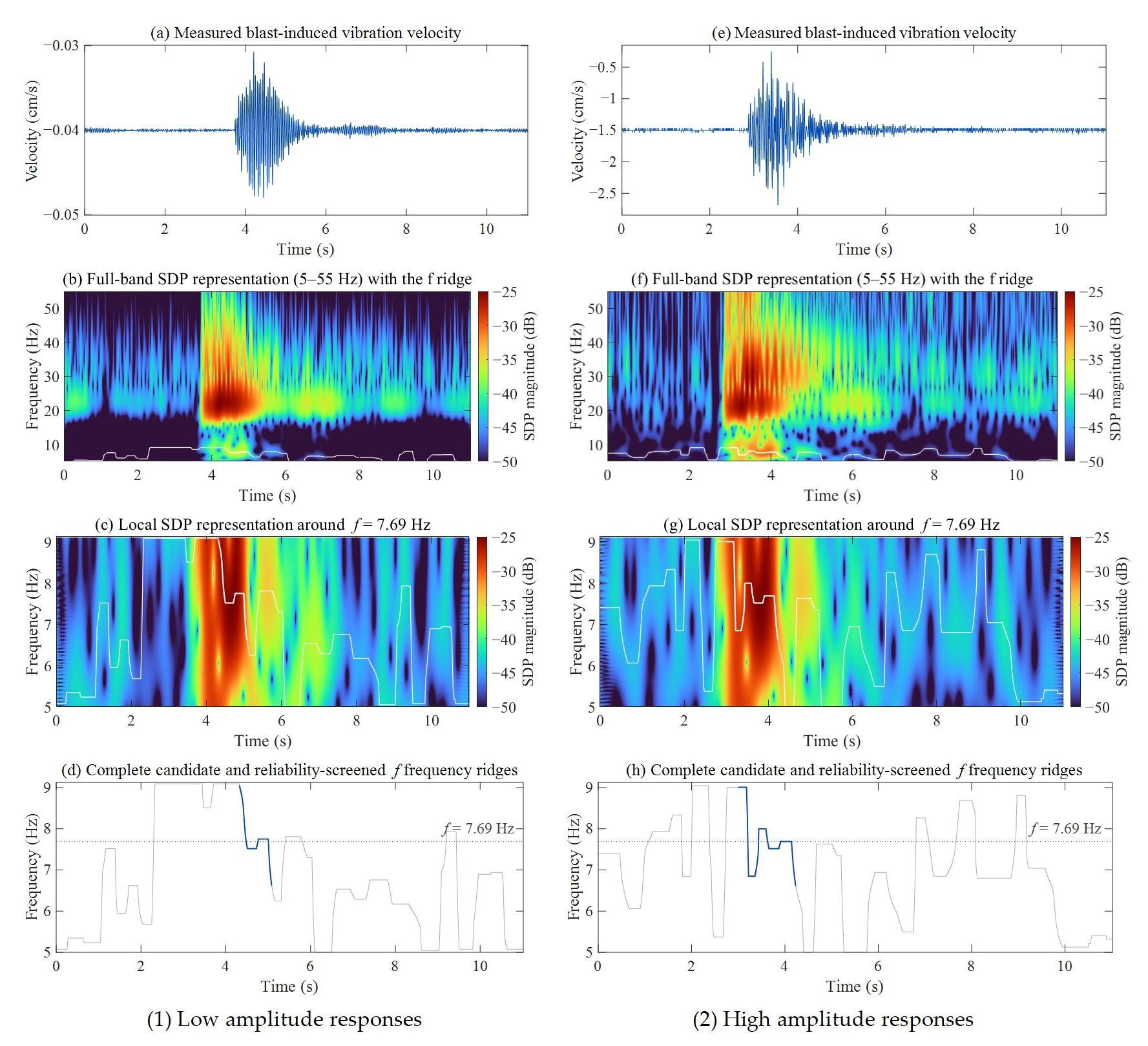
To further examine the non-stationary characteristics of the structural response under blasting excitation, a representative measured blasting record was analyzed using the rationally sampled Stockwell transform (SDP) [41]. The full 5–55 Hz SDP maps were first examined, followed by ridge tracking within the frequency band associated with the first modal cluster f = 7.69 Hz. An SDP-based time-frequency comparison of representative low- and high-amplitude blast-induced responses is shown in Figure 23.

Figure 23. SDP-based time-frequency comparison of representative low- and high-amplitude blast-induced responses.

For both the low- and high-PPV events, the f-associated candidate ridge can be traced before, during, and after the blast response, and transient ridge migration is observed around the strong-motion interval. However, the high-PPV event does not exhibit a clearly larger or more persistent downward migration of the reliability-supported f ridge than the low-PPV event. Therefore, although short-term variations in the f-associated ridge are present in both records, the SDP results do not provide clear evidence of a systematic amplitude-dependent frequency-softening process within the investigated vibration range. This finding is also consistent with the event-to-event f-PPV analysis presented in Section 5.1, which did not reveal a systematic reduction in the identified first-mode frequency with increasing PPV.

5.3. Probability Distribution of Modal Parameters for Brick-Concrete Structure Buildings

(1)

Probability distribution of the identified natural frequency

Based on the above analysis, the identified f exhibit statistical variability among different blasting events without an evident PPV-dependent frequency-softening trend. Therefore, the probability distributions of the identified natural frequencies are further investigated in this section.

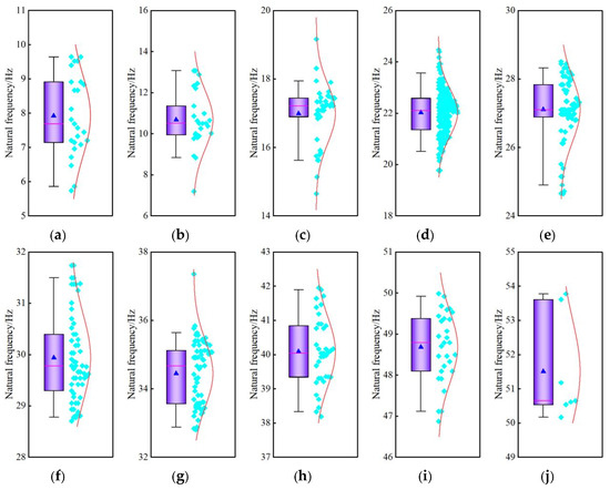
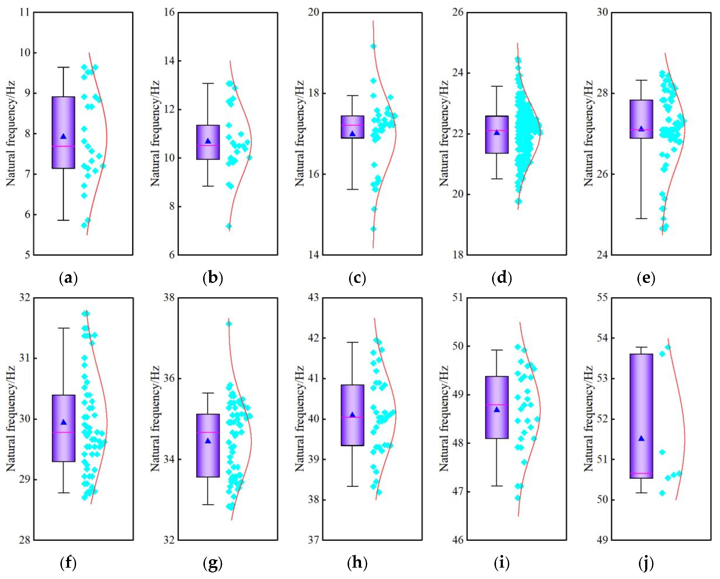
K-means clustering was applied to the natural frequencies identified by the MDCCF method. Based on the clustering results, the frequencies obtained from different response directions were grouped according to frequency order, and the corresponding statistical distributions are presented in Figure 24. The lower-frequency groups exhibit relatively concentrated distributions, whereas greater dispersion is observed in the higher-frequency groups. Because the tangential/radial and vertical components were pooled in the present statistical analysis, the resulting frequency groups may contain contributions from different modal families. Accordingly, Figure 24 should be interpreted as a statistical characterization of grouped identified frequencies rather than as the probability distribution of an individual physical mode. The spectral characteristics of the blasting excitation and the frequency-dependent structural response may also contribute to the differences among the frequency groups. A more detailed separation of direction-dependent modal families and interpretation of the corresponding mode shapes require further investigation.

Figure 24. Distribution of natural frequencies for different orders. (a) First order. (b) Second order. (c) Third order. (d) Fourth order. (e) Fifth order. (f) Sixth order. (g) Seventh order. (h) Eighth order. (i) Ninth order. (j) Tenth order.

As shown in Figure 24, the distribution trends of natural frequency across different orders approximate both normal [42] and Gamma [43] distributions. Therefore, these distributions are employed to model the probability distributions of natural frequencies. The probability density functions for normal and Gamma distributions are presented in (Equation (35)) and (Equation (36)), respectively.

$$F(x)={\displaystyle \frac{1}{\sqrt{2\pi \sigma }}}{e}^{-{\displaystyle \frac{(x-\mu {)}^2}{2{\sigma }^2}}}$$

(35)

where f(x) is the probability density function of a normal distribution, x is the random variable, μ is the mean of the random variable, and σ is the standard deviation of the random variable.

$$g(x/h,z)={\displaystyle \frac{x^{h-1}{e}^{-x/z}}{\mathsf{\Gamma }(h)Z^h}}$$

(36)

where g(x) is the probability density function of the Gamma distribution, $h$ is the shape parameter of the Gamma distribution probability density function, z is the scale parameter of the Gamma distribution probability density function, and Γ($h$) is the Gamma function, as expressed in (Equation (37)).

$$\mathsf{\Gamma }(h)={\int }_0^{\infty }{t}^{h-1}{e}^{-t}dt$$

(37)

The correlation coefficient and root mean square error are used to evaluate the fitting effect of different probability distribution models. It can be expressed as follows:

$$R(X,Y)={\displaystyle \frac{\mathit{Cov}(X,Y)}{\sqrt{V\mathrm{a}\mathrm{r}(X)V\mathrm{a}\mathrm{r}(Y)}}}$$

(38)

X and Y are the random variable, Cov(X, Y) is the covariance of the random variables X and Y, Var(X) is the variance of the random variable X, and Var(Y) is the variance of the random variable Y.

The mean squared error (MSE) is calculated as shown in (Equation (39)).

$$\mathit{MSE}={\displaystyle \frac{1}{N}}\sum _{i=1}^N(X_i-Y_i{)}^2$$

(39)

where N is the sample size of the random variable, X_i is the true value of the ith random variable sample, and Y_i is the predicted value of the ith random variable sample.

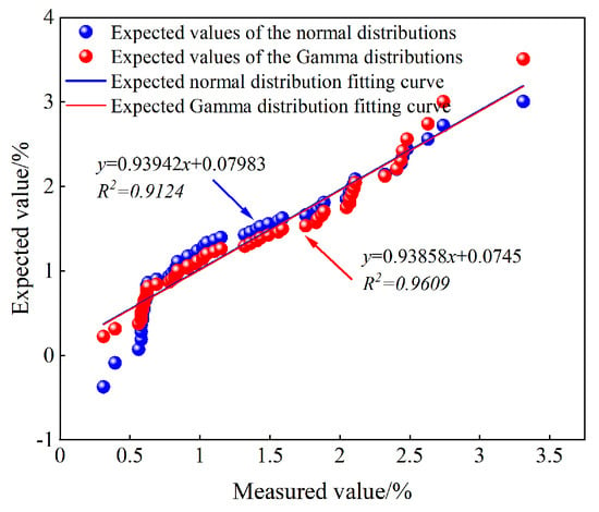
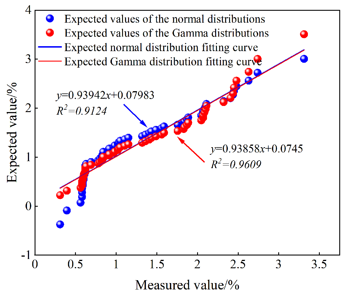
The Q–Q plots of the probability distributions of the first and sixth-order natural frequencies are shown in Figure 25 and Figure 26, respectively, and the Q–Q fitting results for the probability distributions of different-order natural frequencies are presented in Table 12. As shown in Figure 25 and Figure 26 and Table 12, the data points fitted by the normal and Gamma distributions are approximately distributed along the reference line. The differences in the correlation coefficients and root mean square errors obtained from the two distributions are relatively small, indicating that neither fitting model exhibits an obvious advantage over the other. The Gamma distributions have relatively large shape parameters, indicating that their distributional forms are close to the normal distribution. Therefore, the identified natural frequencies can be approximately described by a normal distribution.

Figure 25. Q-Q plot of the first natural frequency probability distribution.

Figure 26. Q-Q plot of the sixth-order natural frequency probability distribution.

Table 12. Q-Q plot fitting results of probability distribution of natural frequencies for different orders.

Order	Normal Distribution				Gamma Distribution
	Mean	Standard Deviation	$\mathit{R}$	MSE	Form Parameter	Scale Parameter	$\mathit{R}$	MSE
1	7.92141	1.18702	0.97784	0.24593	45.316	0.1748	0.97389	0.26405
2	11.0019	1.12674	0.93269	0.40219	104.29077	0.10549	0.94106	0.36041
3	16.98789	0.86426	0.94554	0.27876	386.38762	0.04397	0.94219	0.28694
4	22.02402	0.91585	0.99664	0.07472	577.98694	0.0381	0.99604	0.08112
5	27.10561	0.93925	0.95141	0.28721	824.20345	0.03289	0.948	0.29838
6	29.93861	0.85789	0.97031	0.20804	1252.17622	0.02391	0.97217	0.1988
7	34.44786	0.96738	0.96921	0.23647	1289.90411	0.02671	0.96942	0.23365
8	40.08892	1.01468	0.98924	0.14704	1605.72582	0.02497	0.98938	0.14401
9	48.68034	0.85579	0.98363	0.15264	3333.66487	0.0146	0.98273	0.15446
10	51.50481	1.52413	0.88139	0.72877	1352.11462	0.03809	0.88377	0.66335

(2)

Probability distribution of damping ratio

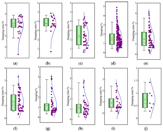
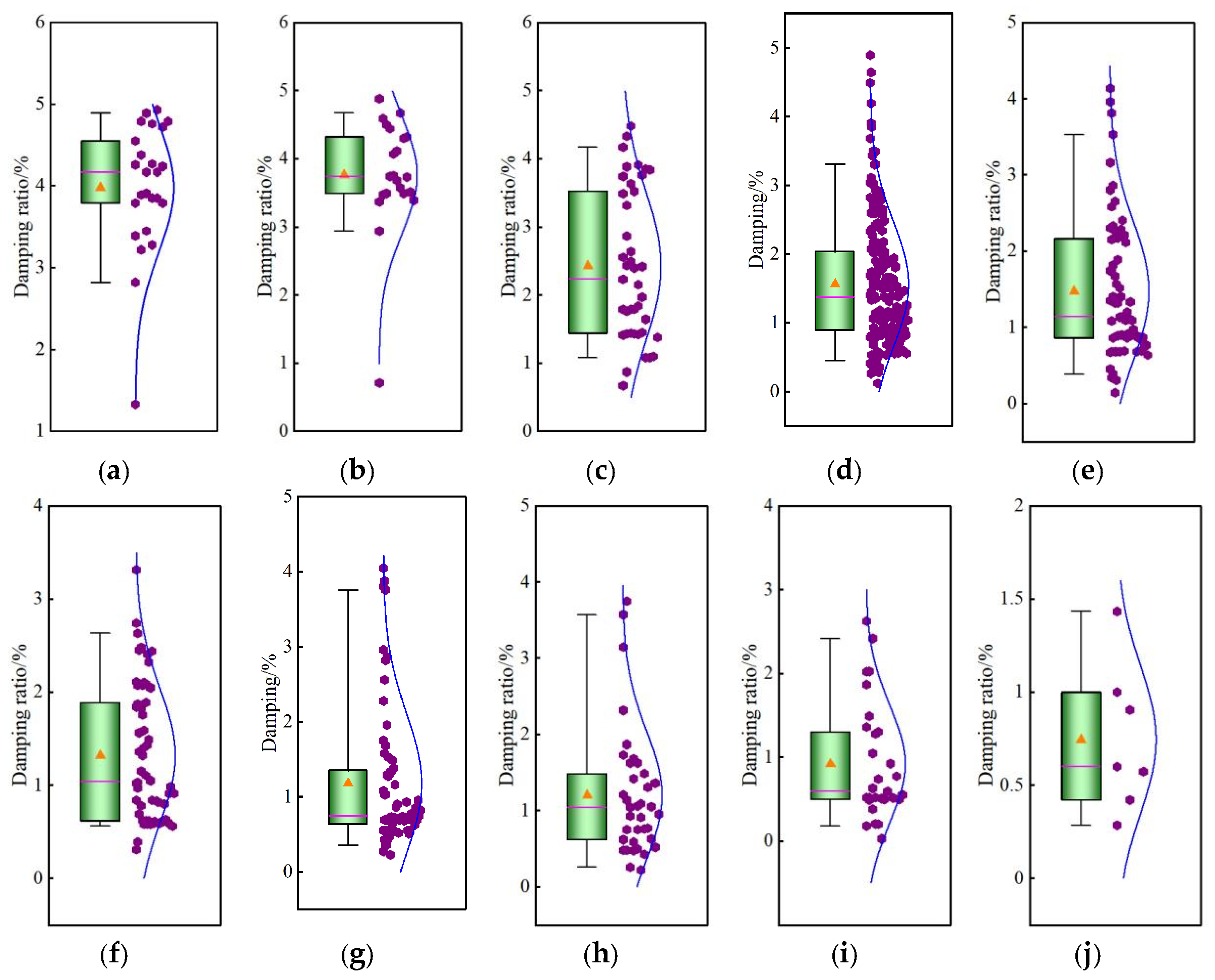
The damping ratio distributions were evaluated according to frequency-cluster membership. Specifically, for each identified frequency cluster, the damping ratios associated with the samples assigned to that cluster were extracted and statistically analysed. The clustering analysis of damping ratios corresponding to different natural frequencies reveals the distribution ranges of various damping ratios as shown in Figure 27. Low-order damping ratios exhibit higher values with relatively concentrated distribution. With increasing order numbers, damping ratios gradually decrease while their distribution range expands. This indicates that brick-concrete structures demonstrate distinct energy dissipation characteristics across different modal vibrations. Specifically, the global vibration modes of low-order modes facilitate efficient energy dissipation, whereas the localized vibration modes of high-order modes struggle to achieve comparable energy dissipation levels.

Figure 27. Distribution of damping ratios for different orders. (a) First order. (b) Second order. (c) Third order. (d) Fourth order. (e) Fifth order. (f) Sixth order. (g) Seventh order. (h) Eighth order. (i) Ninth order. (j) Tenth order.

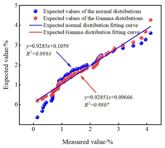
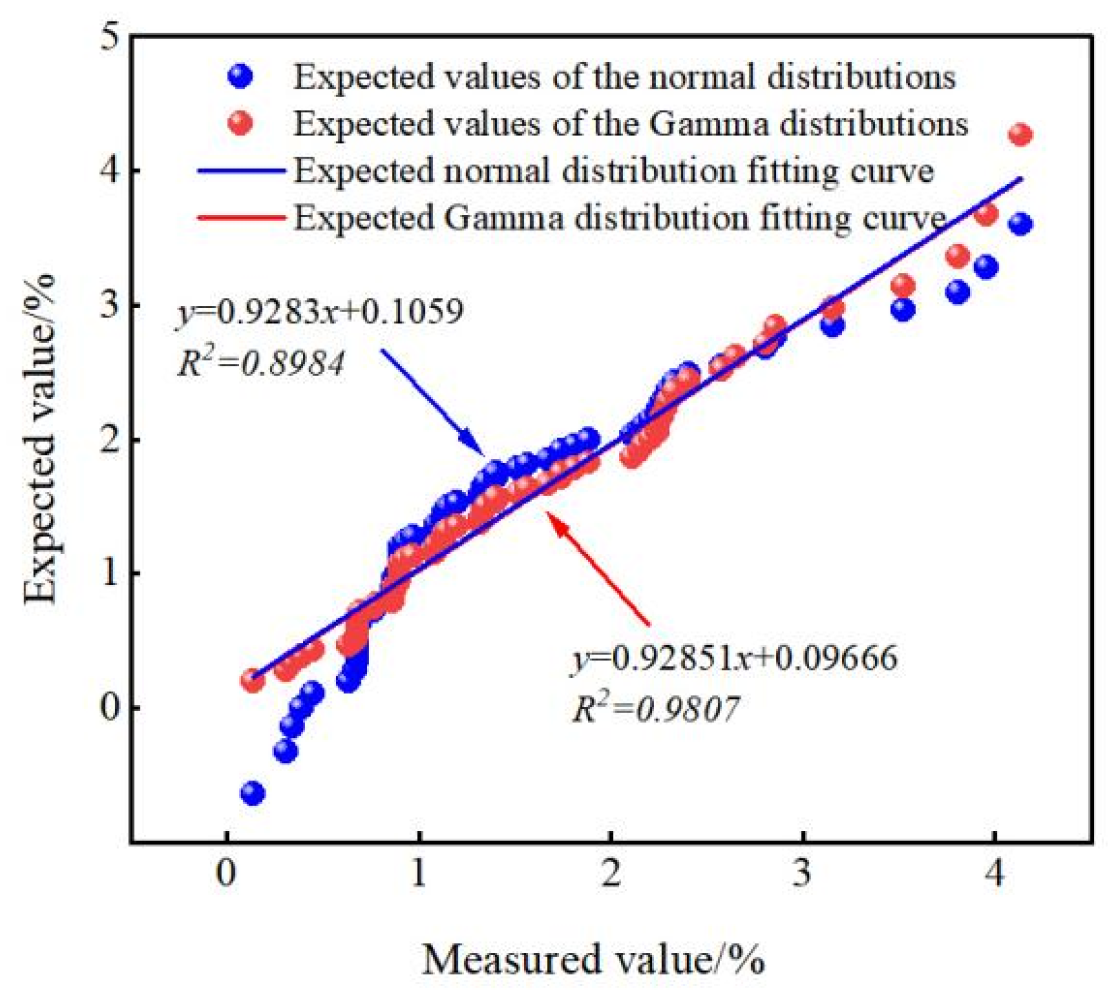
The Q-Q plots of the fifth and sixth order damping ratio probability distributions are shown in Figure 28 and Figure 29, respectively, with fitting results presented in Table 13. There is a significant difference in the fitting performance between normal distribution and Gamma distribution. The normal distribution demonstrates limitations when fitting data across different damping order ratios, as the tail data fails to align with the corresponding reference lines, with most tail data deviating from the reference lines at both ends. In contrast, the Gamma distribution Q-Q plots for different damping order ratios show data points concentrated near the reference lines and arranged in a linear pattern, indicating strong linear relationships. This demonstrates good consistency between the Gamma distribution and the data points across different damping order ratios.

Figure 28. Q-Q plot of the fifth-order damping ratio probability distribution.

Figure 29. Q-Q plot of the sixth-order damping ratio probability distribution.

Table 13. Q-Q plot fitting results of probability distribution of different damping ratios.

Order	Normal Distribution				Gamma Distribution
	Mean	Standard Deviation	$\mathit{R}$	MSE	Form Parameter	Scale Parameter	$\mathit{R}$	MSE
1	3.9796	0.79501	0.92972	0.28976	18.3546	0.21682	0.89931	0.40078
2	3.75995	0.85094	0.87985	0.40023	10.64588	0.35318	0.84285	0.6102
3	2.42455	1.09998	0.96857	0.27113	4.70041	0.51582	0.96832	0.27425
4	1.55338	0.91772	0.96448	0.24159	2.6407	0.58824	0.99747	0.06742
5	1.47697	0.907	0.94785	0.28707	2.8234	0.52312	0.9901	0.12125
6	1.31787	0.73382	0.9552	0.2155	3.33422	0.39526	0.98029	0.14005
7	1.1665	0.94033	0.8794	0.44439	2.07445	0.56232	0.96474	0.20845
8	1.2025	0.84514	0.91077	0.34568	2.53154	0.47501	0.97476	0.16423
9	0.92126	0.69862	0.93546	0.24443	1.66771	0.55241	0.98235	0.12813
10	0.74527	0.39323	0.97193	0.09364	4.19744	0.17755	0.99078	0.04857

As shown in Table 13, the correlation coefficient R and MSE between different damping ratios show significant differences when fitted with normal and Gamma distributions. The Gamma distribution model demonstrates a clear advantage over the normal distribution, with most R values exceeding 0.96 and markedly smaller MSE errors. Comprehensive analysis indicates that the probability distribution of different damping ratios better conforms to the Gamma distribution.

5.4. Quantification of Modal Parameter Uncertainty in Brick-Concrete Structure Buildings

In modal parameter identification, uncontrollable factors such as environmental excitation, measurement errors, and limited sample sizes reduce the accuracy of point estimates, resulting in inevitable statistical fluctuations in dynamic characteristic identification. As critical indicators of structural modal parameters, the mean values of natural frequencies and damping ratios directly affect the engineering applicability of identification results through their statistical stability and confidence interval estimation. Therefore, quantifying the uncertainty of natural frequencies and damping ratios is essential for enhancing the reliability of modal parameter identification.

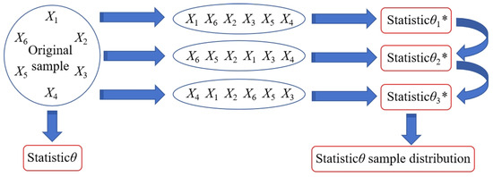
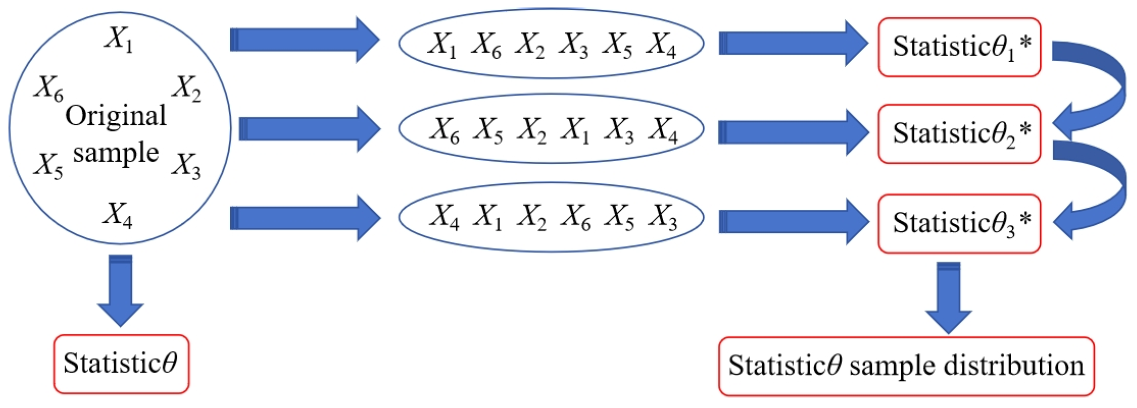
When the population parameter F is unknown, the existing sample data with capacity n is drawn from the population. A sample of capacity n is then randomly selected using the repeated sampling method. The estimation of the population parameters through multiple repeated samples is termed the non-parametric bootstrap method. As a classic non-parametric statistical approach, the bootstrap method demonstrates robustness and stability, effectively estimating the mean confidence interval of modal parameters and compensating for the uncertainty inherent in point estimates. The random sampling process of the bootstrap method is illustrated in Figure 30.

Figure 30. Bootstrap method random sampling. “*” indicates that the sample comes from a Bootstrap resampling rather than the original observed sample.

Using the brick-concrete structure as an example, the bootstrap method is employed to estimate the mean confidence interval of modal parameters, with the following basic steps [27,44]:

(1) Suppose X = (x₁, x₂, x₃, …, x_n) is a sample observation of the overall distribution F(x) of natural frequencies for brick-concrete structures. The estimation error H_a1 and H_a2 of the mean μ and variance σ² are, respectively, as follows:

$$H_{a_1}=\overline{X}-\mu$$

(40)

$$H_{a_2}=S^2-{\sigma }^2$$

(41)

(2) Repeatedly sample W times from the empirical distribution function F_n of the natural frequency X to obtain new samples X_j^∗ (j = 1, 2, 3, ⋯, W). The bootstrap statistics for H_a1 and H_a2 are, respectively, as follows:

$${K_{a_1}}^{\ast }=\overline{X^{\ast }}-\overline{X}$$

(42)

$$K_{a_2}={S^{\ast }}^2-S^2$$

(43)

$${\overline{X}}^{\ast }={\displaystyle \frac{1}{W}}\sum _{j=1}^W\overline{{X_j}^{\ast }}$$

(44)

$$S^{\ast }=\sqrt{{\displaystyle \frac{1}{W-1}}\sum _{j=1}^W{({x_j}^{\ast }-\stackrel{\_}{X^{\ast }})}^2}$$

(45)

(3) Rearrange the natural frequencies (x₁, x₂, x₃, …, x_n) in ascending order to obtain the new sequence Y = (x₁^*, x₂^*, x₃^*, …, x_n^*), where x_i^* denotes the natural frequency in the new sequence. Construct the empirical distribution function F_n(x) as follows:

$$F_n\left(x\right)=\left\{\begin{array}{cc}0& x<x_{(1)}\\ {\displaystyle \frac{i}{n}}& x_{(i)}<x<x_{(i+1)}\\ 1& x\ge x_{(n)}\end{array} i=1, 2, 3, \dots n-1\right.$$

(46)

(4) Based on the sample empirical distribution function F_n(x), the first bootstrap sample is obtained through random sampling. After sampling W times iteratively, the matrix H containing W bootstrap samples is obtained as follows:

$$H=X^{\ast }=({X_1}^{*}, {X_2}^{\ast }, {X_3}^{\ast }, \cdots , {X_W}^{*})=\left[\begin{array}{cccc}{x}_{11}^{\ast }& x_{11}^{\ast }& \cdots & x_{1W}^{\ast }\\ x_{21}^{\ast }& x_{22}^{\ast }& \cdots & x_{2W}^{\ast }\\ \cdot & \cdot & \cdot & \cdot \\ x_{n1}^{\ast }& x_{n2}^{\ast }& \cdots & x_{\mathrm{nW}}^{\ast }\end{array}\right]$$

(47)

(5) Calculate the mean ${\overline{X_j}}^{\ast }$ and variance ${S^{\ast }}^2$ of the bootstrap sample ${X_j}^{\ast }$. The bootstrap mean $\stackrel{\wedge }{\mu }$ and variance $\stackrel{\wedge }{{\sigma }^2}$ distributions are $\stackrel{\wedge }{\mu }=(\stackrel{\wedge }{{\mu }_1}, \stackrel{\wedge }{{\mu }_2}, \dots , \stackrel{\wedge }{{\mu }_W})$ and $\stackrel{\wedge }{{\sigma }^2}=(\stackrel{\wedge }{{{\sigma }_1}^2}, \stackrel{\wedge }{{{\sigma }_2}^2}, \dots , \stackrel{\wedge }{{{\sigma }_W}^2})$, respectively. The bootstrap statistic ${K_a}^{\ast }$ is the estimate of $H_a$.

(6) Plot the frequency distribution histogram of $\stackrel{\wedge }{\mu }$ and $\stackrel{\wedge }{{\sigma }^2}$, where $F_n(\stackrel{\wedge }{\mu })$ and $F_n(\stackrel{\wedge }{{\sigma }^2})$ are replaced by $F_n(\mu )$ and $F_n({\sigma }^2)$.

(7) The percentile method is used to estimate the mean interval.

(8) Define the correction factor β. ${\mathsf{\Phi }}^{-1}\left[.\right]$ is the inverse function of the standard normal distribution, and $I(\overline{X_j^{\ast }})$ is the indicator function.

$$\beta ={\mathsf{\Phi }}^{-1}\left[{\displaystyle \frac{1}{W}}\sum _{j=1}^{W}I(\stackrel{\_}{{X_j}^{\ast }})\right]$$

(48)

$$I\left(\overline{X_j^{\ast }}\right)=\left\{\begin{array}{cc}1& \overline{X_j^{\ast }}\le \overline{X}\\ 0& \overline{X_j^{\ast }}>\overline{X}\end{array}\right.$$

(49)

(9) The confidence intervals corresponding to the bias-corrected percentile [45] interval method are [k_a, k_b]. $\mathrm{a}=\mathsf{\Phi }({2\beta +\mathrm{z}}_{\alpha /2})$, $\mathrm{b}=\mathsf{\Phi }({2\beta +\mathrm{z}}_{1-\alpha /2})$.

The mean uncertainty of the first natural frequency of a brick-concrete structure is quantified by using the MDCCF method. The first natural frequency samples are X₁ = (6.714, 9.6436, 8.911, 9.399, 5.737, 7.202, 7.812, 8.117, 7.69, 6.958, 9.522, 8.667, 9.522, 5.859, 6.469, 7.1411, 7.3242, 9.643, 7.5684, 7.08, 8.667, 7.446, 8.911, 7.202, 8.8299). The mean value is 7.9214 Hz, and the variance is 1.409 Hz².

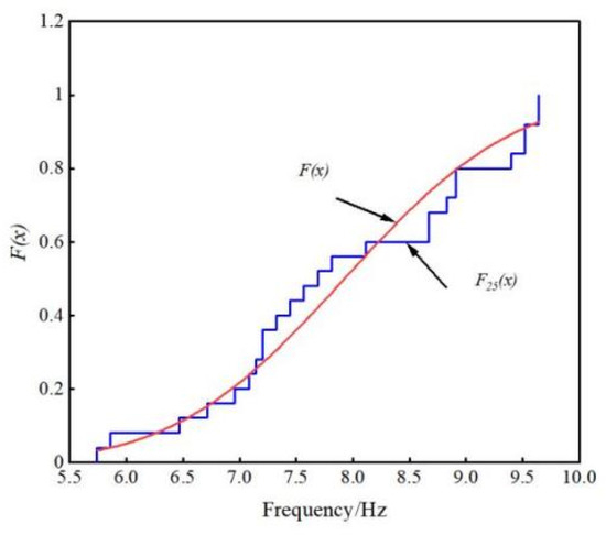
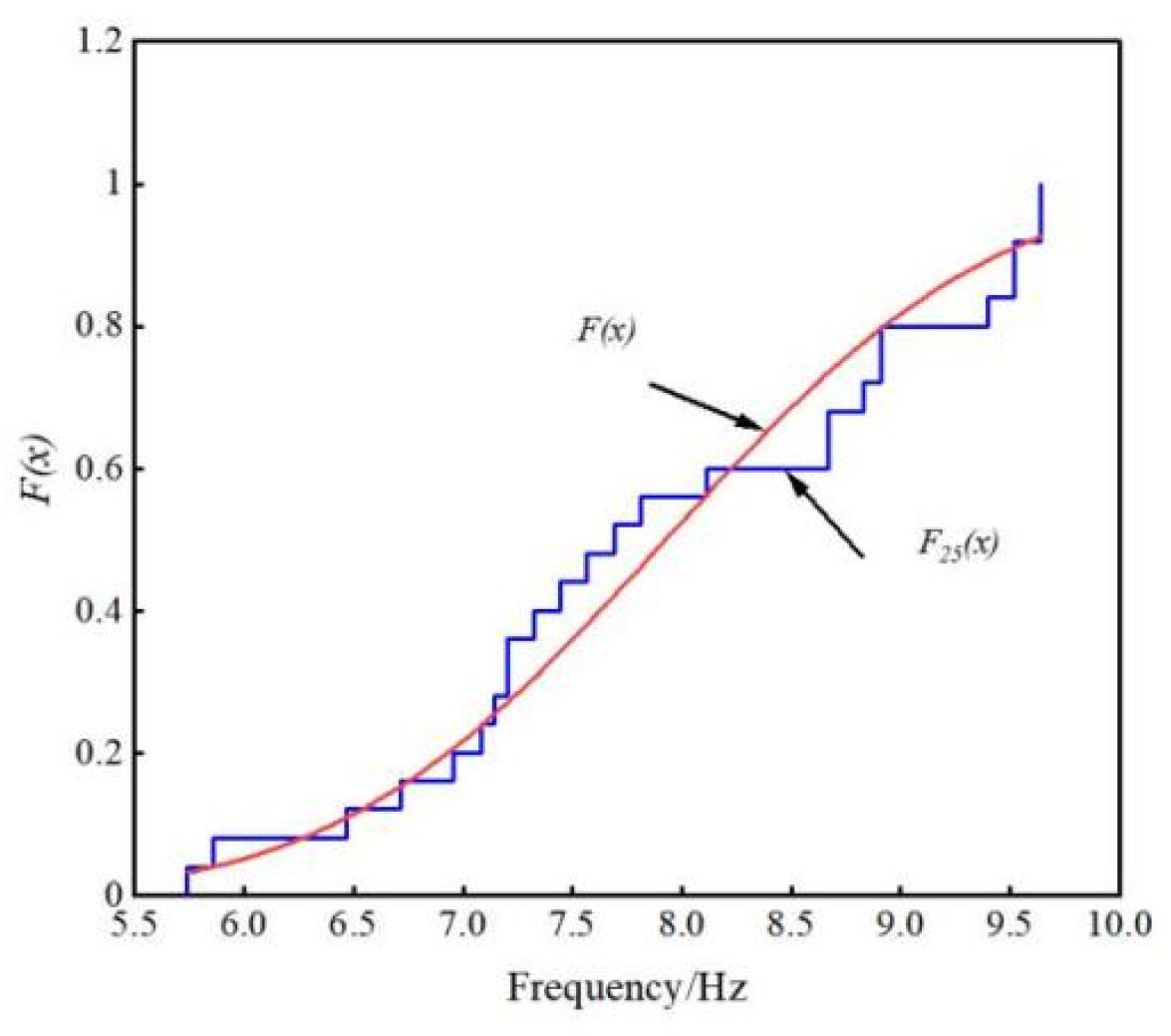
The bootstrap method exhibits significant randomness during repeated sampling. To ensure the reproducibility of mean confidence interval estimates for natural frequencies, the random seed was set to 123. Figure 31 compares the empirical distribution function of bootstrap resampled samples with the theoretical one. The empirical distribution function demonstrates discontinuity in morphology, yet its overall trend has initially converged with the theoretical distribution. This indicates that the empirical distribution function constructed by the bootstrap method effectively captures the sample’s distribution characteristics.

Figure 31. Empirical distribution function.

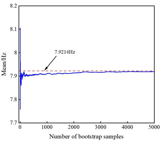
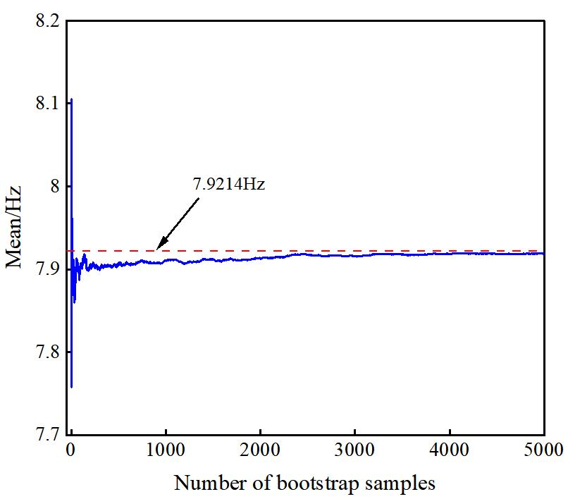
Figure 32 illustrates the variation in the mean of bootstrap sample means with increasing sampling frequency. The data reveals that at low sampling frequencies, the mean exhibits significant fluctuations, demonstrating notable numerical instability—a characteristic reflecting high variance in initial sample mean estimation. As the number of resampling iterations increases, particularly beyond 3000 iterations, the mean of bootstrap sample means stabilizes and converges toward the original sample mean, confirming the asymptotic consistency of the bootstrap method in estimating natural frequency means.

Figure 32. Mean change curve of the bootstrap sample mean.

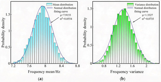
The bootstrap resampling was conducted 3000 times. The mean and variance of 3000 bootstrap samples were statistically analyzed. The frequency distribution histograms of the bootstrap sample mean and variance for sample X₁ are shown in Figure 33. The mean and variance of the bootstrap sample follow normal distributions N(7.9155, 0.2354²) and N(1.3527, 0.2711²), respectively. The mean and variance of the bootstrap sample are essentially consistent with those of the original sample, indicating that the bootstrap sample effectively inherits the fundamental characteristics of the original sample X₁.

Figure 33. Frequency distribution histogram of bootstrap sample mean and variance for the sample X1. (a) Mean. (b) Variance.

Using the bias-corrected percentile interval method, the 95% confidence interval for the population mean of the sample X₁’s natural frequency is estimated as [7.4725, 8.3811]. The same methodology was applied to estimate confidence intervals for other-order natural frequencies and damping ratios. The confidence interval results for the mean natural frequencies and damping ratios of brick-concrete structures are presented in Table 14 and Table 15. As shown in these tables, the bootstrap analysis provides 95% confidence intervals for the natural frequencies and damping ratios identified by the MDCCF method, thereby quantifying the statistical uncertainty associated with the identified modal parameters.

Table 14. Confidence interval estimation results of the natural frequency for the brick-concrete structure building.

Order	Natural Frequency/Hz	Bootstrap Method Confidence Interval/Hz
		Lower Limit	Superior Limit
1	7.69	7.4725	8.3811
2	10.559	10.5988	11.5284
3	17.2068	16.7046	17.2270
4	22.095	21.9032	22.1444
5	27.099	26.8705	27.2973
6	29.7741	29.7333	30.1725
7	34.668	34.2188	34.6808
8	40.039	39.7692	40.4053
9	48.7882	48.3591	48.9778
10	50.6476	50.6301	52.8201

Table 15. Confidence interval estimation of the damping ratio for the brick-concrete structure building.

Order	Damping Ratio/%	Bootstrap Confidence Interval
		Superior Limit	Lower Limit
1	4.4602	4.5725	4.3774
2	3.705	3.7081	3.59
3	2.8618	2.9556	2.858
4	2.4161	2.4675	2.3921
5	1.9	1.9715	1.9
6	1.45	1.5026	1.4516
7	1.11	1.131	1.098
8	0.8579	0.8603	0.832
9	0.59	0.6059	0.5767
10	0.3493	0.3562	0.2932

6. Conclusions

Using the proposed MDCCF modal parameter identification method, an experiment was conducted to identify the modal parameters of a brick-concrete structure building subjected to blasting action, with deep-hole blasting in an open-pit mine as the excitation source. The candidate natural frequencies and damping ratios of the brick-concrete structural building are defined, and the probability distribution and confidence interval are revealed. The main conclusions are as follows:

(1)

Compared with the results of the SSI-cov-K-means method and PP-K-means method, the natural frequency and damping ratio of the five-story frame structure numerical model identified by the MDCCF method are closer to the theoretical values, with errors within 1% and 3%, respectively, and the maximum errors are 0.52% and 2.45%. This method can effectively identify the true modal parameters of the structure, demonstrating high accuracy and engineering application value.

(2)

The candidate modal parameters of the brick-concrete structure under deep-hole blasting in an open-pit mine were identified by the MDCCF method. The candidate natural frequencies are 7.69 Hz, 10.559 Hz, 17.2068 Hz, 22.095 Hz, 27.099 Hz, 29.7741 Hz, 34.668 Hz, 40.039 Hz, 48.7882 Hz, and 50.6476 Hz, and the candidate damping ratios are 4.4602%, 3.705%, 2.8618%, 2.4161%, 1.9%, 1.45%, 1.11%, 0.8579%, 0.59%, and 0.3493%.

(3)

The candidate natural frequency and damping ratio of the brick-concrete structure house are well distributed by normal distribution and Gamma distribution, respectively. The candidate natural frequencies and damping ratios identified by the MDCCF method show overall agreement with the corresponding 95% bootstrap confidence intervals for the mean values. This provides a quantitative characterization of the uncertainty in the identified candidate natural frequencies and damping ratios of brick-concrete structures.

(4)

The identified frequency groups are regarded as candidate modal frequencies rather than confirmed global structural modes and require further validation through additional measurements or independent modal testing.

References

- Wang, H.L.; Zhao, Y.; Shan, R.L.; Wei, Y.H.; Liu, D.; Dong, J. Safety evaluation and application of blasting vibration based on an improved Hilbert–Huang transform. Rock Mech. Rock Eng. 2023, 56, 3971–3991. [Google Scholar] [CrossRef] [Scilit]
- Nateghi, R. Evaluation of blast induced ground vibration for minimizing negative effects on surrounding structures. Soil Dyn. Earthq. Eng. 2012, 43, 133–138. [Google Scholar] [CrossRef] [Scilit]
- Zhao, Y.; Shan, R.L.; Wang, H.L. Blasting vibration effect and safety evaluation method of railway cross tunnels. Tunn. Undergr. Space Technol. 2024, 145, 105588. [Google Scholar] [CrossRef] [Scilit]
- Garai, D.; Agrawal, H.; Mishra, A.K. Impact of orientation of blast initiation on ground vibrations. J. Rock Mech. Geotech. Eng. 2023, 15, 255–261. [Google Scholar] [CrossRef] [Scilit]
- Kong, L.H.; Yan, P.; Liu, X.; Lu, W.B.; Zhou, C.; Gao, Q.Y.; Yang, X.S.; Li, M. Estimating the mechanical and dynamic parameters in surrounding rock mass of tunnels based on velocities of blasting seismic waves. Tunn. Undergr. Space Technol. 2025, 165, 106897. [Google Scholar] [CrossRef] [Scilit]
- Yang, S.L.; Liu, Z.C.; Wang, S.F.; Zhong, W.; Zhang, R.; Yao, X.H. Dynamic response and failure analysis for urban bridges under far-field blast loads. Eng. Struct. 2023, 285, 116043. [Google Scholar] [CrossRef] [Scilit]
- Gou, Y.G.; Shi, L.Z.; Huo, X.F.; Yu, Z.; Chen, Y.M. Propagation and prediction of blasting vibration on ground surface induced by underground mining with comparison to vibration inside rock. Rock Mech. Rock Eng. 2024, 57, 10283–10306. [Google Scholar] [CrossRef] [Scilit]
- Patnaik, G.; Rajput, A. Safety assessment of underground steel pipelines with CFRP protection against subsurface blast loading. Structures 2023, 54, 1541–1559. [Google Scholar] [CrossRef] [Scilit]
- Daryan, A.S.; Soleimani, S.; Ketabdari, H. A modal nonlinear static analysis method for assessment of structures under blast loading. J. Vib. Control 2018, 24, 3631–3640. [Google Scholar] [CrossRef] [Scilit]
- Bayraktar, A.; Altunişik, A.C.; Özcan, M. Safety assessment of structures for near-field blast-induced ground excitations using operational modal analysis. Soil Dyn. Earthq. Eng. 2012, 39, 23–36. [Google Scholar] [CrossRef] [Scilit]
- Sales, N.M.; Chang, C.M. Improved operational modal analysis by modified data-driven stochastic subspace identification featuring visualization. Mech. Syst. Signal Process. 2025, 237, 113071. [Google Scholar] [CrossRef] [Scilit]
- Bao, Y.Q.; Liu, D.W.; Li, H. A mechanics-informed neural network method for structural modal identification. Mech. Syst. Signal Process. 2024, 216, 111458. [Google Scholar] [CrossRef] [Scilit]
- Zhou, K.; Zhi, L.H.; Wang, J.F.; Hong, X.; Xu, K.; Shu, Z.R. An improved stochastic subspace modal identification method considering uncertainty quantification. Structures 2023, 51, 1083–1094. [Google Scholar] [CrossRef] [Scilit]
- Ablitzer, F. Peak-picking method for identifying natural frequencies and damping ratios from free vibration measurements. Acta Acust. 2026, 10, 18. [Google Scholar] [CrossRef] [Scilit] [PubMed]
- Brincker, R.; Zhang, L.M.; Andersen, P. Modal identification of output-only systems using frequency domain decomposition. Smart Mater. Struct. 2001, 10, 441–445. [Google Scholar] [CrossRef] [Scilit]
- Guo, Y.; Kareem, A. Non-stationary frequency domain system identification using time-frequency representations. Mech. Syst. Signal Process. 2016, 72–73, 712–726. [Google Scholar] [CrossRef] [Scilit]
- Xu, C.; Wang, C.; Liu, W. Nonstationary vibration signal analysis using wavelet-based time-frequency filter and wigner-ville distribution. J. Vib. Acoust. 2016, 138, 051009. [Google Scholar] [CrossRef] [Scilit]
- Yan, B.F.; Miyamoto, A.; Brühwiler, E. Wavelet transform-based modal parameter identification considering uncertainty. J. Sound Vib. 2006, 291, 285–301. [Google Scholar] [CrossRef] [Scilit]
- Bahar, O.; Ramezani, S. Enhanced Hilbert-Huang transform and its application to modal identification. Struct. Des. Tall Spec. Build. 2014, 23, 239–253. [Google Scholar] [CrossRef] [Scilit]
- Dziedziech, K.; Czop, P.; Staszewski, W.J.; Uhl, T. Combined non-parametric and parametric approach for identification of time-variant systems. Mech. Syst. Signal Process. 2018, 103, 295–311. [Google Scholar] [CrossRef] [Scilit]
- Stockwell, R.G.; Mansinha, L.; Lowe, R.P. Localization of the complex spectrum: The S transform. IEEE Trans. Signal Process. 1996, 44, 998–1001. [Google Scholar] [CrossRef] [Scilit]
- Cole, H.A. On-Line Failure Detection and Damping Measurement of Aerospace Structures by Random Decrement Signatures; NASA: Washington, DC, USA, 1973. Available online: https://ntrs.nasa.gov/citations/19730010202 (accessed on 20 January 2026).
- Van Overschee, P.; De Moor, B. Subspace algorithms for the stochastic identification problem. Automatica 1993, 29, 649–660. [Google Scholar] [CrossRef] [Scilit]
- Greś, S.; Riva, R.; Süleyman, C.Y.; Andersen, P.; Łuczak, M.M. Uncertainty quantification of modal parameter estimates obtained from subspace identification: An experimental validation on a laboratory test of a large-scale wind turbine blade. Eng. Struct. 2022, 256, 114001. [Google Scholar] [CrossRef] [Scilit]
- Pan, H.; Li, Y.; Deng, T.; Fu, J. An improved stochastic subspace identification approach for automated operational modal analysis of high-rise buildings. J. Build. Eng. 2024, 89, 109267. [Google Scholar] [CrossRef] [Scilit]
- Xu, K.; Li, Q.-S.; Zhou, K.; Han, X.-L. A bootstrap-based stochastic subspace method for modal parameter identification and uncertainty quantification of high-rise buildings. J. Build. Eng. 2024, 87, 109007. [Google Scholar] [CrossRef] [Scilit]
- Silva, E.; Magluta, C.; Roitman, N.; Filho, L.A. Development of a structural identification methodology with uncertainty quantification through the SSI and bootstrap techniques. Mech. Syst. Signal Process. 2022, 165, 108290. [Google Scholar] [CrossRef] [Scilit]
- Peeters, B.; De Roeck, G. Reference-based stochastic subspace identification for output-only modal analysis. Mech. Syst. Signal Process. 1999, 13, 855–878. [Google Scholar] [CrossRef] [Scilit]
- Magalhães, F.; Cunha, Á.; Caetano, E. Online automatic identification of the modal parameters of a long span arch bridge. Mech. Syst. Signal Process. 2009, 23, 316–329. [Google Scholar] [CrossRef] [Scilit]
- Reynders, E.; Houbrechts, J.; De Roeck, G. Fully automated (operational) modal analysis. Mech. Syst. Signal Process. 2012, 29, 228–250. [Google Scholar] [CrossRef] [Scilit]
- Liu, W.; Yang, N.; Bai, F.; Law, S.-S.; Abruzzese, D. An improved automated framework for operational modal analysis with multi-stage clustering and modal quality evaluation. Mech. Syst. Signal Process. 2024, 212, 111235. [Google Scholar] [CrossRef] [Scilit]
- Romanazzi, A.; Scocciolini, D.; Savoia, M.; Buratti, N. Iterative hierarchical clustering algorithm for automated operational modal analysis. Autom. Constr. 2023, 156, 105137. [Google Scholar] [CrossRef] [Scilit]
- Ni, P.; Yin, Z.; Han, Q.; Du, X. Output-only structural identification with random decrement technique. Structures 2023, 51, 55–66. [Google Scholar] [CrossRef] [Scilit]
- Shi, C.; Wei, B.; Wei, S.; Wang, W.; Liu, H.; Liu, J. A quantitative discriminant method of elbow point for the optimal number of clusters in clustering algorithm. EURASIP J. Wirel. Commun. Netw. 2021, 2021, 31. [Google Scholar] [CrossRef] [Scilit]
- Lu, X.; He, X.; Chen, H.; Zheng, R. Operational modal parameter identification with colored noise excitation. Chin. J. Aeronaut. 2021, 34, 288–300. [Google Scholar] [CrossRef] [Scilit]
- Huang, J.; Li, X.; Zhang, J.; Sun, Y.; Ren, J. Determining the Rayleigh damping parameters of flexible pavements for finite element modeling. J. Vib. Control 2022, 28, 3181–3194. [Google Scholar] [CrossRef] [Scilit]
- Liu, W.; Yang, N.; Bai, F.; Chang, P. Parameter optimization of covariance-driven stochastic subspace identification method based on sensitivity analysis. Eng. Mech. 2021, 38, 157–167+178. [Google Scholar] [CrossRef]
- Maharana, K.; Mondal, S.; Nemade, B. A review: Data pre-processing and data augmentation techniques. Glob. Transit. Proc. 2022, 3, 91–99. [Google Scholar] [CrossRef] [Scilit]
- Al-Khamees, H.A.A.; Al-Slivani, M.M.; Kadhim, M.S.; Radhi, A.D.; Sani, N.S.; Al-Amri, R.M.; Wahit, F.; Sani, M.A.A. Enhancing classification accuracy in medical datasets using a hybrid distance and cluster refinement-based K-means clustering method. Sci. Rep. 2026, 16, 3490. [Google Scholar] [CrossRef] [Scilit] [PubMed]
- Mao, J.X.; Wang, H.; Fu, Y.G.; Spencer, B.F., Jr. Automated modal identification using principal component and cluster analysis: Application to a long-span cable-stayed bridge. Struct. Control Health Monit. 2019, 26, e2430. [Google Scholar] [CrossRef] [Scilit]
- Ditommaso, R.; Ponzo, F.C. Time-frequency representation of nonlinear structural response through rationally sampled Stockwell analysis. Mech. Syst. Signal Process. 2026, 260, 114920. [Google Scholar] [CrossRef] [Scilit]
- Leipus, R.; Šiaulys, J.; Dirma, M.; Zovė, R. On the distribution-tail behaviour of the product of normal random variables. J. Inequal. Appl. 2023, 2023, 32. [Google Scholar] [CrossRef] [Scilit]
- Chen, P.; Buis, K.; Zhao, X. A comprehensive toolbox for the gamma distribution: The gammadist package. J. Qual. Technol. 2023, 55, 75–87. [Google Scholar] [CrossRef] [Scilit]
- Efron, B.; Tibshirani, R.J. An Introduction to the Bootstrap; Chapman & Hall: New York, NY, USA, 1993. [Google Scholar]
- Efron, B.; Narasimhan, B. The automatic construction of Bootstrap confidence intervals. J. Comput. Graph. Stat. 2020, 29, 608–619. [Google Scholar] [CrossRef] [Scilit] [PubMed]
Disclaimer/Publisher’s Note: The statements, opinions and data contained in all publications are solely those of the individual author(s) and contributor(s) and not of MDPI and/or the editor(s). MDPI and/or the editor(s) disclaim responsibility for any injury to people or property resulting from any ideas, methods, instructions or products referred to in the content. |
© 2026 by the authors. Licensee MDPI, Basel, Switzerland. This article is an open access article distributed under the terms and conditions of the Creative Commons Attribution (CC BY) license.