Room Temperature Prediction for District Heating Substation Control: Integrating CatBoost Solar Radiation Prediction and State-Space Modeling

Abstract

In district heating systems, the large-scale deployment of room temperature collectors has accumulated massive amounts of terminal data, but these data mostly remain at the level of viewing and statistical analysis and have not been effectively connected to real-time control of district heating substations. As a direct reflection of thermal comfort, room temperature can be incorporated into predictive control of district heating substations, which can promote the transition of heating control from lagging compensation to proactive prediction. To address three engineering bottlenecks, namely, the lack of solar radiation information, significant differences in user thermal characteristics, and the accumulation of prediction errors, this paper proposes a rolling room temperature prediction method that integrates CatBoost solar radiation prediction, canonical variate analysis (CVA) subspace identification, and adaptive Kalman filtering. Based on representative users selected by clustering, a model predictive control framework with an alternating iterative solution strategy is constructed to directly serve the closed-loop control of district heating substations. The method relies only on conventional weather forecasts and existing data collected by the heating system, without additional hardware costs. Taking a residential community in Luoyang as an example, there were 490 valid users on the prediction day of 16 December 2024. Using data from the 15 days prior to the prediction day for training and hourly rolling prediction, the root mean square error (RMSE) and mean absolute error (MAE) for all users were 0.203 °C and 0.146 °C, respectively, and the RMSE under six typical weather conditions remained within 0.21 °C. Online computation only involves low-dimensional matrix operations, and the computational burden is small, demonstrating the potential for deployment on existing controllers of district heating substations and good engineering deployability.

1. Introduction

As the core infrastructure for winter heating in northern cities, district heating systems have long been operated and controlled with heat sources and district heating substations as the center, and the supply water temperature is usually set according to an empirical compensation curve based on outdoor air temperature [1,2,3]. This open-loop control mode responds with a lag. After weather changes, room temperature fluctuates, and adjustment can often be implemented only after the room temperature has deviated from the comfort range for several hours [4,5]. With the advancement of carbon peaking and carbon neutrality goals and the increasing requirements for energy conservation and emission reduction in the building sector, district heating systems are facing an urgent need to transition from passive balancing to proactive and precise control [6].

In recent years, the penetration rate of heat meters and room temperature collectors at heating terminals has increased substantially, enabling heating enterprises to obtain massive and continuous actual room temperature data [7,8]. However, these data mostly remain at the level of viewing and statistical analysis and have not yet formed effective feedback to district heating substation controllers [9]. As a direct reflection of heating quality, if room temperature can be incorporated into predictive control of district heating substations, it will promote the transition of heating control from lagging compensation to proactive prediction [10,11]. Existing studies have shown that predictive control methods based on room temperature feedback can effectively reduce room temperature fluctuations and achieve energy savings [12,13].

Building reliable room temperature prediction faces three key engineering problems.

Problem 1: Lack of solar radiation information. The heat gain contribution of solar radiation to daytime room temperature in winter cannot be ignored. Under similar outdoor temperature conditions, the rise in room temperature differs significantly on sunny and cloudy days. However, radiation measurement equipment is expensive, and ordinary district heating substations can hardly be equipped with it. Although conventional weather forecasts from meteorological departments do not contain radiation values, they include weather codes, air temperature, humidity, wind speed, and air pressure, which provide a data basis for machine learning-based radiation prediction [14,15,16]. Existing studies have shown that gradient boosting algorithms perform well in handling categorical weather features and nonlinear mapping of meteorological elements [17,18], providing a feasible technical path for radiation prediction without radiation sensors [19,20].

Problem 2: Significant differences in user thermal characteristics. Due to differences in floors, orientations, and building envelopes, the dynamic response time of room temperature to heating parameters differs markedly among users [21]. If a unified model is applied to all users, the prediction accuracy for some users will inevitably be low. Therefore, it is necessary to extract a personalized thermal dynamic model from the historical operation data of each user. Subspace identification methods can automatically extract state-space models from input–output data without presetting the model order, making them particularly suitable for dynamic modeling of multi-input coupled systems [22,23,24,25]. Related studies have applied subspace identification to building thermal dynamic modeling, verifying its feasibility for large-scale deployment [26,27].

Problem 3: Accumulation and amplification of prediction errors. Errors inevitably exist in sensors and model predictions. Without hourly measured correction, prediction deviations will rapidly accumulate and amplify within 24 h [28]. Kalman filtering can effectively suppress error accumulation by fusing model predictions with measured values at each time step [29,30]. Existing studies have applied extended Kalman filtering to adaptive correction of building thermal models, verifying its robustness to model mismatch [31,32]. On this basis, Bayesian optimization provides an efficient solution for automatic tuning of filtering parameters, avoiding the cumbersome process of manual debugging [33].

To address the above problems, this paper proposes a data-driven framework that integrates outdoor meteorological features, terminal room temperature data, and district heating substation operation parameters. The main work of this paper includes the following three aspects. First, CatBoost 1.2.10 is used to perform nonlinear mapping of conventional weather forecast elements, achieving hourly solar radiation prediction without radiation sensors and providing accurate radiation boundary conditions for subsequent room temperature modeling. Second, a canonical variate analysis (CVA) subspace identification method is introduced to automatically extract a thermal dynamic state-space model from the historical operation data of each user without manually presetting the model order. The model complexity can be adaptively determined according to the actual response characteristics of users, making it suitable for batch deployment in large-scale district heating systems. Third, Bayesian optimization is used to adaptively tune the Kalman filtering parameters for each user. In the offline stage, the prediction error on the validation set is taken as the objective function to search for the optimal combination of process noise and measurement noise. After obtaining the steady-state Kalman gain, only simple matrix operations are required, which do not increase the online computational burden and achieve real-time optimal fusion of model prediction and measured room temperature. The value of room temperature prediction lies in providing advance decision-making support for district heating substation control. Therefore, on the basis of the hourly room temperature prediction model, this paper further constructs a rolling optimization control framework for predictive control of district heating substations, so the prediction results can be directly converted into adjustment instructions for supply water temperature and branch flow rate. The above prediction and control framework was validated on real data from 490 valid users in a residential community in Luoyang on 16 December 2024. The prediction results can be directly sent to the district heating substation controller at each hourly time instant, demonstrating engineering deployability.

2. Data Preprocessing and Overall Framework

2.1. Data Preprocessing

After raw room temperature data are collected and uploaded, short-term missing data, communication anomalies, and sensor noise are inevitable. To ensure the stability of state-space identification and filtering, the time axis of each household time series is first aligned, data with continuous missing values exceeding 6 h are removed, short-term missing values are filled by linear interpolation, and individual jump points exceeding physical thresholds are corrected using a sliding window median.

Considering that room temperature changes have significant slow-varying characteristics, the Symlets8 wavelet basis is used for five-level decomposition, and a soft thresholding function is employed to remove high-frequency random noise. The soft thresholding function is:

$$\lambda =\sigma \sqrt{2\ln N}$$

where N is the signal length and σ is the noise standard deviation. This processing can effectively reduce the interference of noise on CVA subspace identification without affecting the model’s perception of room temperature dynamics in the prediction stage. After wavelet filtering, the room temperature curve retains the main rising and falling trends and peak information, while high-frequency noise is effectively eliminated, providing a clean data foundation for subsequent state-space identification. It should be noted that interpolation and wavelet denoising are performed only on the historical data within the training window, which is entirely prior to the prediction day. In the online rolling prediction stage, the Kalman filter update at each time step uses only the current measured room temperature, and no future information is introduced. Therefore, the preprocessing does not cause information leakage.

2.2. Overall Framework of the Method

The service object of room temperature prediction is the hourly predictive control of district heating substations. At each hourly time instant, the district heating substation controller needs to know what room temperature response the current control strategy will produce at the next time step. Therefore, the method in this paper is executed cyclically with one hour as the basic time unit.

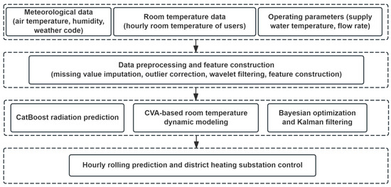
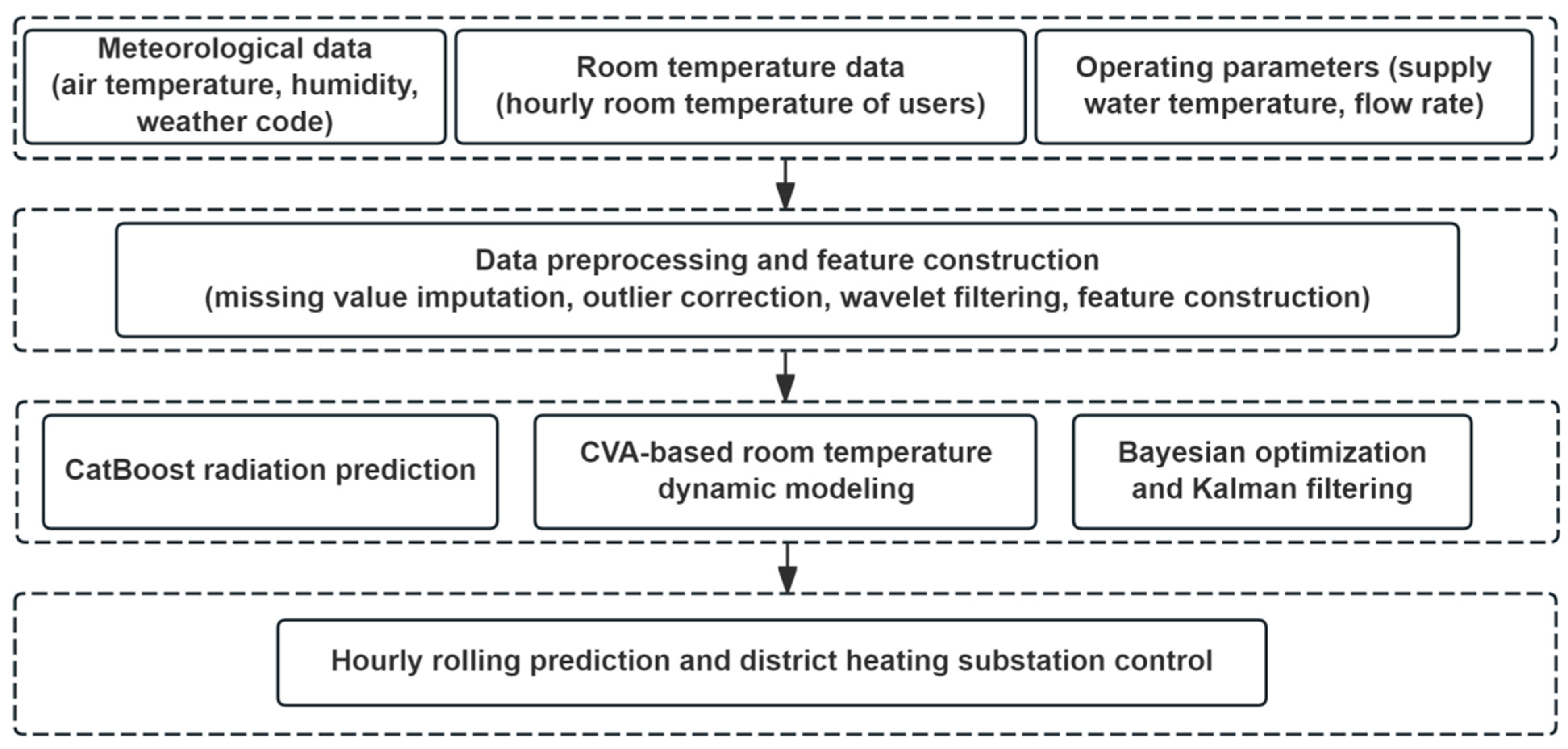
The method consists of two modules. The first is the model establishment module, which is divided into global and local levels. At the global level, historical meteorological data from three complete heating seasons (15 November 2021 to 15 March 2024) are used to pretrain the CatBoost solar radiation prediction model. At the local level, historical data from the 15 days prior to the prediction day are used to establish a personalized state-space model for each user and optimize the filtering parameters. The model establishment module is retrained once per day, and clustering is performed once per day to select representative users for prediction, so as to adapt to the slow changes in building thermal characteristics during the heating season. The second is the hourly prediction module, which obtains the latest weather forecast and current measured room temperature at each hourly time instant, performs one-step prediction, and sends the prediction results to the district heating substation controller. The overall technical route of the proposed method is shown in Figure 1.

Figure 1. Overall technical route of the room temperature prediction method. The dashed boxes represent the different modules (data, preprocessing, core algorithm, and control) of the proposed framework.

All input data for the entire method come from existing collection systems, without additional hardware. The data sources include hourly historical room temperature data of each household, supply water temperature of the district heating substation, branch flow rates of users, outdoor air temperature, relative humidity, WMO weather codes, and European ECMWF ERA5 reanalysis solar radiation data (used for offline training).

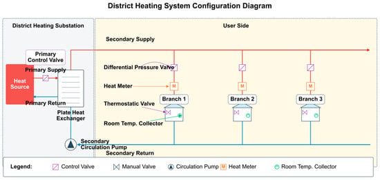
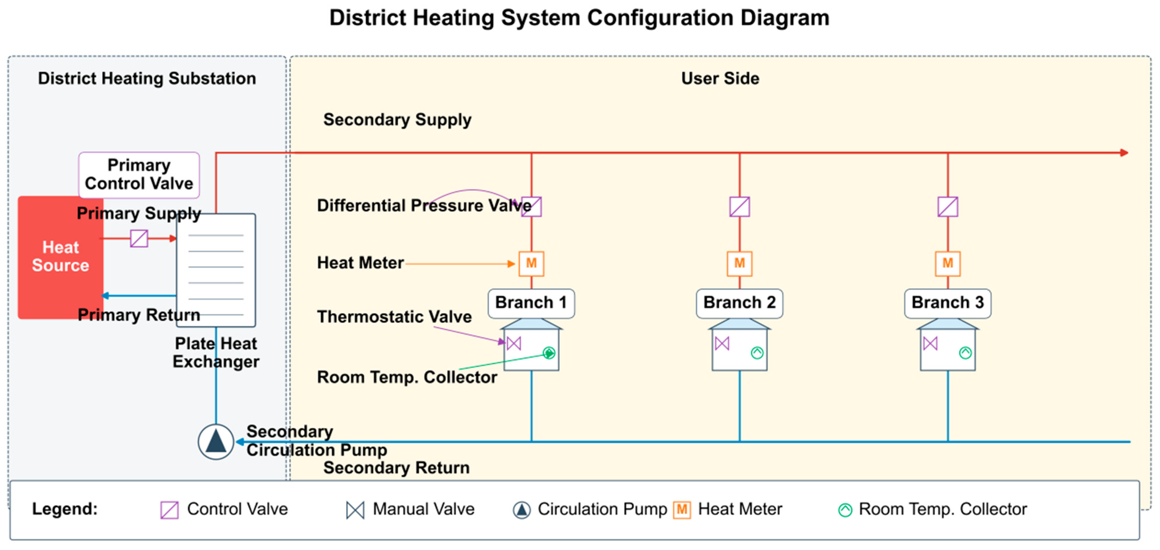
The configuration of the studied district heating system, including the heat source, substation, secondary-side supply and return pipes, user branches, control valves, and room temperature collectors, is shown in Figure 2.

Figure 2. District heating system configuration diagram with control valve positions. The red and blue lines represent the supply and return pipes, respectively, and the arrows indicate the flow direction.

3. CatBoost-Based Solar Radiation Prediction

Solar radiation is an important additional heat source for daytime room temperature in winter. Under the same outdoor temperature, the rise in room temperature differs significantly on sunny and cloudy days. Professional radiometers are difficult to configure in ordinary district heating substations, and conventional weather forecasts do not directly provide solar irradiance at the required temporal and spatial resolution. Therefore, the CatBoost model is used to convert conventional weather forecast elements into hourly solar radiation prediction values. If measured or forecast solar irradiance is available, it can be directly used as an input, and the proposed framework is fully compatible with such a case.

3.1. Model Training and Feature Construction

The training data are derived from hourly meteorological records of three complete heating seasons (November 2021 to March 2024), totaling 8736 valid samples. The solar radiation labels are obtained from the European ECMWF ERA5 reanalysis dataset. The input features include relative humidity, solar elevation angle, sine of hour, cosine of hour, and WMO weather code, totaling five dimensions. The core advantage of the CatBoost algorithm lies in its native support for categorical features. Traditional boosting algorithms need to expand weather codes into one-hot vectors, which leads to high-dimensional sparsity. In contrast, CatBoost directly handles categorical variables through ordered target encoding, enabling more effective learning of the nonlinear mapping of different weather codes to radiation attenuation. The main hyperparameters of the model are set as follows: number of trees = 500, maximum depth = 6, learning rate = 0.05, and early stopping rounds = 20.

3.2. Accuracy Evaluation and Comparison of the Radiation Prediction Model

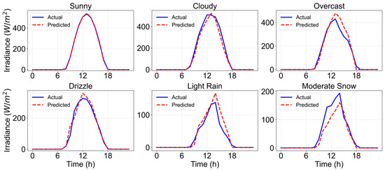
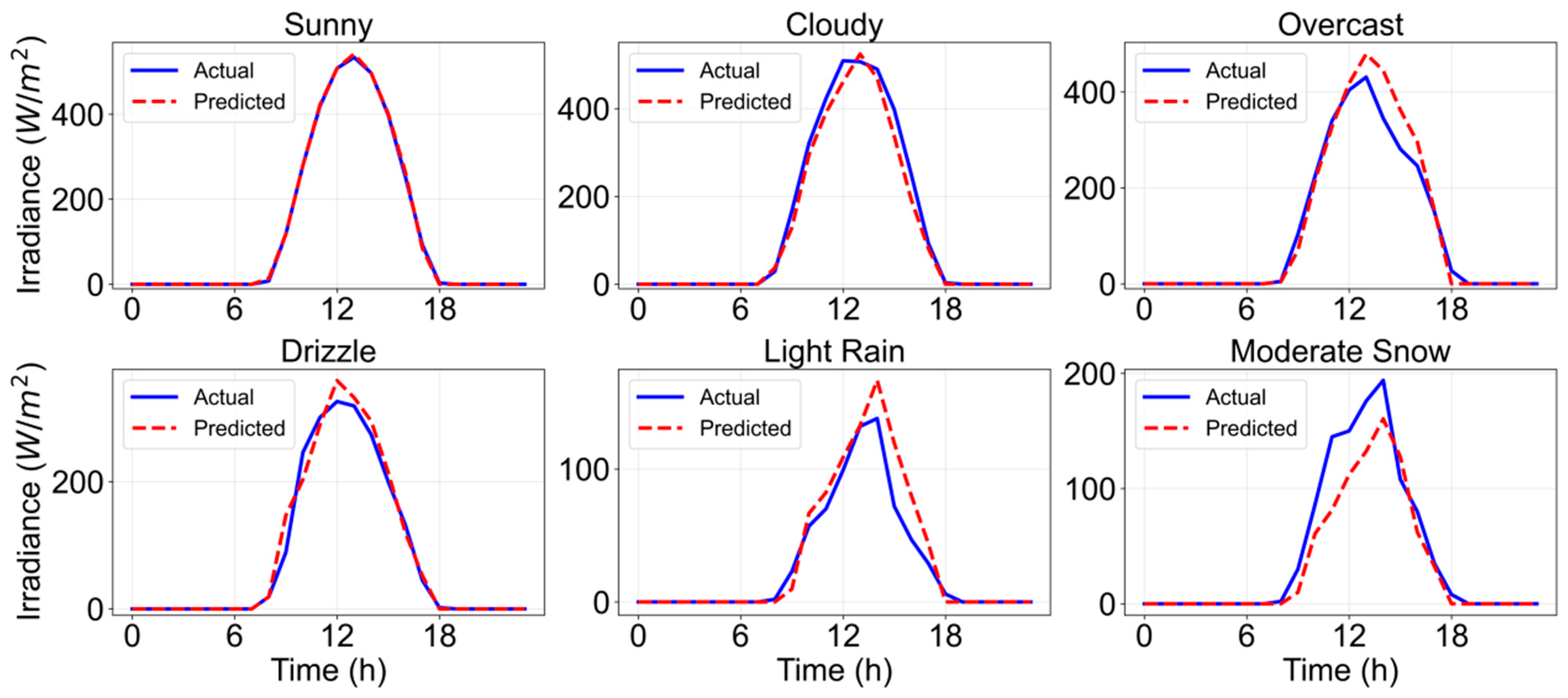
The model is evaluated on an independent test set (15 November 2024 to 15 March 2025, the entire heating season, totaling 2904 samples). The results show that the root mean square error (RMSE) for the entire heating season is 39.26 W/m², the mean absolute error (MAE) is 18.02 W/m², and the coefficient of determination (R²) is 0.9610. Figure 3 shows a comparison between hourly solar radiation prediction values and true values under six typical weather conditions (sunny, cloudy, overcast, light drizzle, light rain, and moderate snow) during the heating season. It can be seen that the model can accurately track the radiation peak during high-radiation periods at noon on sunny days and also capture the radiation fluctuation trend well under complex weather such as overcast, rainy, and snowy conditions. The predicted values are forced to zero at night, which is consistent with physical laws.

Figure 3. Comparison between hourly solar radiation prediction values and true values under six typical weather conditions.

To verify the rationality of selecting CatBoost, this paper compares it with XGBoost, LightGBM, Random Forest, MLP neural network, the traditional Kt lookup table method, and pure clear-sky theoretical radiation. All comparisons are conducted on the 2024–2025 heating season test set. To ensure fairness, all machine learning models use the same five-dimensional feature input, in which weather codes are processed by one-hot encoding. The comparison results are shown in Table 1.

Table 1. Performance comparison of seven solar radiation prediction methods (fair comparison setting).

Model Name	Category	RMSE (W/m2)	MAE (W/m2)	R2
CatBoost (unified one-hot encoding)	Gradient boosting	40.40	18.02	0.961
XGBoost	Gradient boosting	40.90	17.59	0.958
LightGBM	Gradient boosting	41.21	17.82	0.957
Random Forest	Bagging	42.63	17.85	0.954
MLP neural network	Neural network	42.34	22.79	0.955
Kt lookup table method	Traditional method	134.97	32.24	0.538
Pure clear-sky theoretical radiation	Theoretical method	234.04	134.19	−0.388

The accuracy of the four ensemble learning methods is highly consistent, with all RMSE values between 40 and 43 W/m². Under the fair comparison setting of unified one-hot encoding, CatBoost achieves the best performance with an RMSE of 40.40 W/m². The final model in this paper adopts the native categorical feature processing of CatBoost, that is, weather codes are directly input as categorical variables rather than one-hot expanded. The RMSE is further reduced to 39.26 W/m², and R² is 0.9610, which is still superior to the other models. The MLP neural network performs second best, with an RMSE of 42.34 W/m², but it is still significantly better than the traditional methods. The error of the traditional Kt lookup table method is as high as 134.97 W/m², about 3 times that of the machine learning methods. The RMSE of pure clear-sky theoretical radiation reaches 234.04 W/m², and R² is negative, indicating that it is infeasible to predict radiation solely by solar geometry if weather attenuation is ignored. Based on the above comparative analysis, this paper finally selects CatBoost as the core model for radiation prediction. To objectively evaluate the above error level, it is considered in the corresponding physical magnitude: the instantaneous peak solar radiation at noon on sunny days during the heating season in Luoyang can generally reach 500–600 W/m², and the error proportion of the CatBoost model’s RMSE relative to the peak radiation intensity is only about 7%.

To further explain the rationality and necessity of the model input features, feature ablation experiments are conducted by removing individual features one by one and retraining the model, and the changes in test set RMSE are observed. The experimental results are shown in Table 2.

Table 2. Feature ablation experiment results.

Removed Feature	RMSE (W/m2)	ΔRMSE (W/m2)
All retained (baseline)	39.26	0
Solar elevation angle	56.36	+17.11
WMO weather code	50.67	+11.41
Cosine of hour	43.63	+4.37
Relative humidity	41.84	+2.58
Sine of hour	39.37	+0.11

Based on the ablation experimental results, the contribution of each feature to model performance shows a clear hierarchical structure. The removal of solar elevation angle leads to an increase of 17.11 W/m² in RMSE, making it the most influential single feature, which verifies the fundamental role of solar–terrestrial geometry in radiation prediction. The removal of WMO weather code leads to an increase of 11.41 W/m² in RMSE, indicating that cloud and precipitation states have an irreplaceable characterization effect on radiation attenuation. The removal of cosine of hour leads to an increase of 4.37 W/m² in RMSE, verifying the importance of day–night boundary truncation for zero nighttime radiation prediction. The removal of relative humidity leads to an increase of 2.58 W/m² in RMSE, indicating that humidity, as a key parameter of atmospheric scattering, participates in the correction of radiation attenuation. The removal of sine of hour has the smallest impact on model accuracy, with ΔRMSE of only 0.11 W/m², but it still makes a positive contribution and, together with cosine of hour, forms a complete description of the day–night phase.

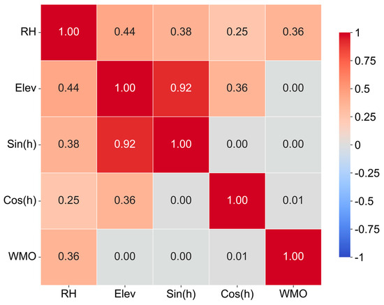
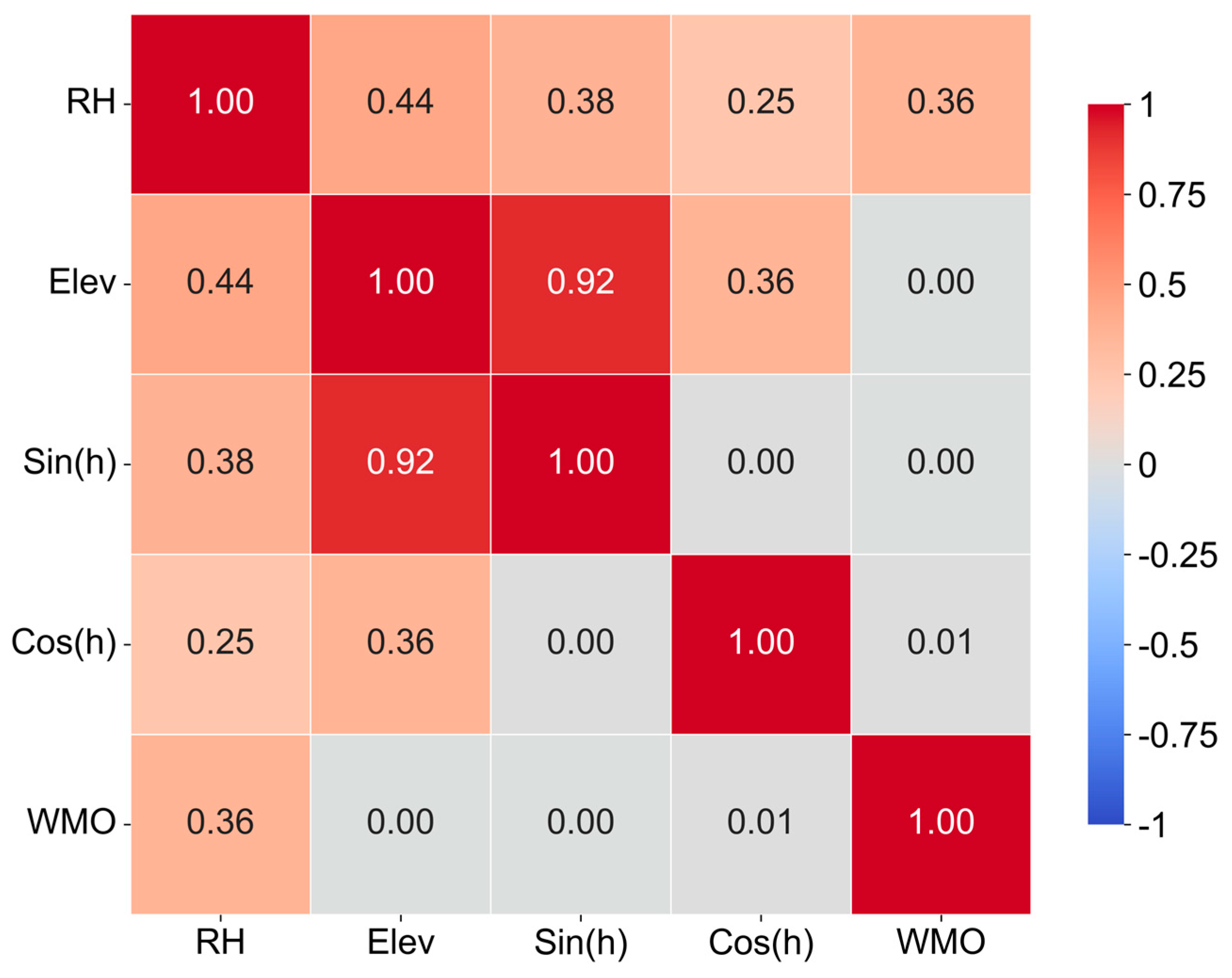
To further verify the rationality of the feature set, this paper conducts a Pearson correlation analysis on the five input features, and the results are shown in Figure 4. Overall, the correlation coefficients among the features are generally low. Only solar elevation angle and sine of hour show an extremely high positive correlation, with an r value of 0.919. This is because the solar elevation angle itself is calculated from the astronomical geometric relationship at the observation time, while sine of hour is a mathematical mapping of the same time on a periodic basis. The two are inevitably coupled by astronomical geometry. For tree models, this collinearity does not cause parameter pathology, and the feature ablation experiment confirms that removing sine of hour only increases RMSE by 0.11 W/m². There is no significant correlation between the other feature pairs, indicating that the feature set provides complementary information from three independent dimensions, namely, solar–terrestrial geometry, atmospheric scattering, and cloud state, and there are no redundant features. This paper finally adopts a five-dimensional concise feature set, with a model RMSE of 39.26 W/m², MAE of 18.02 W/m², and R² of 0.9610.

Figure 4. Pearson correlation coefficient matrix of features. RH: relative humidity; Elev: solar elevation angle; Sin(h): sine of hour; Cos(h): cosine of hour; WMO: World Meteorological Organization weather code.

It should be noted that the ERA5 reanalysis dataset is used as the reference for solar radiation in this study. ERA5 provides gridded model outputs rather than direct surface radiometric measurements and may contain systematic biases due to urban aerosols, local fog, or cloud cover variations. Therefore, the reported RMSE of 39.26 W/m² quantifies the agreement between CatBoost and ERA5, rather than the absolute accuracy against ground-level irradiance in Luoyang. These biases can propagate into the state-space model through the radiation input. However, the Kalman filter uses hourly measured room temperature to correct the state estimate, which partially suppresses the influence of radiation input errors. The ablation experiment in Section 4.4 shows that removing the radiation input increases the room temperature prediction RMSE by about 12.3%, indicating that solar radiation is beneficial for prediction accuracy even with the uncertainty in ERA5. Future work will consider calibrating ERA5 against local ground measurements to further improve the accuracy of radiation and room temperature prediction.

4. Room Temperature Dynamic Modeling and Adaptive Filtering Prediction

4.1. CVA-Based Personalized State-Space Model Identification

The building thermal characteristics of different users differ significantly. For top-floor corner units, the exterior wall area is large, and the wind pressure effect is strong, so the room temperature responds quickly to heating changes. For middle-floor residents, the room temperature changes relatively gently due to heat conduction from neighboring apartments. If a unified model is used to describe all users, its prediction accuracy will inevitably deviate. This paper uses CVA subspace identification to automatically extract a personalized dynamic response model from the historical data of each user.

The input variables are defined as outdoor air temperature T_amb, supply water temperature of the district heating substation T_c, user branch flow rate flow and CatBoost-predicted radiation R_cat. The output is the single-dimensional room temperature T_room. CVA subspace identification constructs an information matrix with a past window length of s = 10 h, extracts the dynamic modes with the strongest correlation between past and future information, and finally obtains the state-space model:

$$x_{t+1}=A{x}_t+B{u}_{t+1}+w_t$$

$$y_{t+1}=C{x}_{t+1}+D{u}_{t+1}+v_{t+1}$$

where the model order n is adaptively selected from three candidate values: 2, 3, and 4. The CVA state order is determined by enumerating the candidate set {2, 3, 4}: for each candidate order, a Hankel matrix is constructed with past/future window length s = 10, canonical variates are extracted by QR decomposition and SVD, and the state-space matrices are estimated by least squares. Subsequently, one-step open-loop recursive prediction is performed on the training set, the mean square error of room temperature prediction is calculated, and the order with the smallest mean square error is selected as the optimal CVA model order for that user. After similarity transformation, the state vector x_t can correspond to the internal temperature nodes of the building equivalent thermal network (RC network), and its specific physical meaning depends on the transformation matrix obtained by identification. For example, when n = 2, it can correspond to the indoor air temperature node and the exterior wall surface temperature node. When n = 3, a temperature node representing internal thermal mass such as furniture is added to describe the heat exchange between indoor heat capacity and wall heat capacity. When n = 4, it is further refined into a multi-level temperature distribution of the inner and outer wall surfaces and internal thermal mass, which can more precisely capture the temperature gradient along the thickness direction of building envelopes with different orientations. This process does not require manually presetting the topology and can automatically adapt to the significant differences between top-floor corner units (large thermal inertia) and middle-floor units (greatly affected by heat transfer from neighboring apartments).

4.2. Adaptive Kalman Filtering and Bayesian Parameter Optimization

After the state-space model is established, if only open-loop recursion of the model is used, prediction errors will gradually accumulate over time. Kalman filtering can weightedly fuse the model prediction value with the measured value at each time step, correct the internal state estimate, and thereby suppress the hourly accumulation of errors.

The performance of Kalman filtering depends on the process noise covariance matrix Q and the measurement noise covariance matrix R. The optimal Q and R differ significantly among different users. For top-floor corner units, the degree of model mismatch is relatively high, and a larger Q is needed to enhance the response to measured values. For sensors near windows, readings fluctuate greatly due to the influence of the local temperature field, and R should be increased accordingly. If unified parameters are used for all users, the filtering effect for some users will inevitably deviate from the optimum. Therefore, this paper adopts Bayesian optimization to adaptively tune the filtering parameters for each user. To reduce the search dimension, let Q = qI and R = rI, where q and r are scalars. The objective function is defined as the prediction RMSE on the validation set (the last 20% of the training set), and the search is performed 30 times within the ranges q ∈ [10⁻⁶, 10²] and r ∈ [10⁻⁶, 10²]. This offline optimization does not increase the online computational burden. After obtaining the steady-state Kalman gain K, only simple matrix multiplication and addition are required. Compared with grid search, Bayesian optimization has higher search efficiency in high-dimensional spaces. Compared with genetic algorithms, it converges faster and is suitable for parallel deployment in systems with hundreds of users. In each iteration, the algorithm predicts the changing trend of the objective function through a Gaussian process surrogate model and adaptively selects the next sampling point, thereby approaching the optimal solution within 30 iterations.

4.3. Hourly Rolling Prediction Process

The prediction uses one hour as the time step. At each hourly time instant t, the weather forecast for time t + 1 is obtained, the radiation at time t + 1 is calculated by the CatBoost model, and the input vector u_t+1 is formed together with the set values or optimized values of supply water temperature and branch flow rate. Combined with the current state estimate x_t, one-step state prediction and observation prediction are performed:

$$x_{t+1|t}=A{x}_t+B{u}_{t+1}$$

$$y_{t+1|t}=C{x}_{t+1|t}+D{u}_{t+1}$$

The obtained y_t+1|t is the room temperature prediction value at the next time step, which is sent in real time to the district heating substation controller as the basis for predictive adjustment of supply water temperature. When the measured room temperature at time t + 1 arrives, the innovation is calculated and the state is updated. The corrected state is used as the starting point for the next prediction, thereby suppressing the hourly accumulation of errors.

In the above process, the weather forecast for time t + 1 is already available at time t. The supply water temperature and branch flow rate are taken as actual operational parameters or control set values in offline evaluation and are given by model predictive control optimization in online deployment. This setting is consistent with the actual operation of district heating substations, in which future boundary conditions are obtained in advance before control is executed.

4.4. Accuracy Verification and Ablation Experiments of Room Temperature Prediction

Taking 16 December 2024 as the prediction day, data from the 15 days prior to the prediction day are used for training, and four configurations are compared on 490 valid users. The results are shown in Table 3: (1) the complete method (CatBoost + CVA + adaptive Kalman filtering); (2) removing the radiation input; (3) removing Kalman filtering (open-loop recursion); and (4) retaining filtering but using fixed parameters Q = 0.1I, R = 0.1I.

Table 3. Prediction accuracy comparison of four methods.

Method	Average RMSE/°C	Average MAE/°C	RMSE Standard Deviation
Complete method	0.203	0.146	0.133
Removing radiation input	0.228	0.162	0.146
Removing Kalman filtering	0.618	0.527	0.448
Fixed-parameter filtering	0.235	0.166	0.147

The average RMSE of the complete method is 0.203 °C, the average MAE is 0.146 °C, and the standard deviation is 0.133 °C. After removing Kalman filtering, the open-loop recursion RMSE rises sharply to 0.618 °C, more than three times that of the complete method. This fully demonstrates that without measured feedback, the error of the state-space model will rapidly amplify within 24 h. The RMSE of fixed-parameter filtering is 0.235 °C, about 15.7% higher than that of the complete method, indicating that Bayesian adaptive tuning is indeed necessary and that unified parameters will deviate from the optimal operating point of some users. After removing the radiation input, the RMSE rises to 0.228 °C, an increase of about 12.3%, indicating that even during the heating season, the influence of solar radiation on room temperature cannot be ignored.

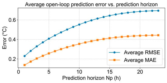
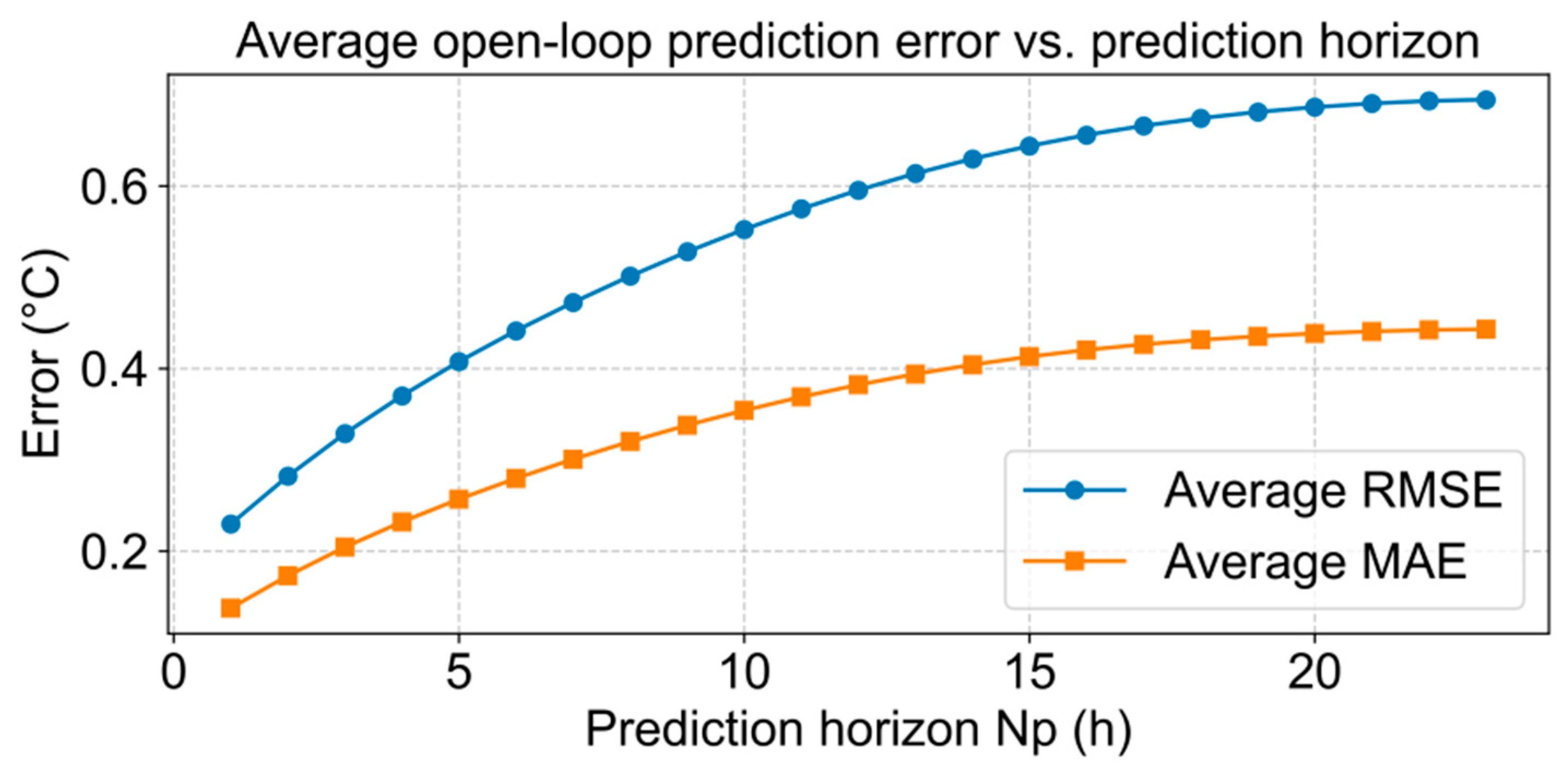
To evaluate the multi-step open-loop prediction capability of the identified CVA model under practical model predictive control conditions, a sensitivity analysis is further conducted. At each time step t, the Kalman filter first updates the state estimate x_t using measurements up to time t. Then, the CVA model performs open-loop prediction from x_t for future horizons of 1 to 24 h without any further measurement updates. For each prediction horizon N_p, the average RMSE and MAE over all users and all starting time steps are calculated. The results are shown in Figure 5.

Figure 5. Average open-loop prediction error versus prediction horizon N_p.

The results show that the average RMSE is 0.230 °C for N_p = 1 h, 0.329 °C for N_p = 3 h, 0.442 °C for N_p = 6 h, 0.596 °C for N_p = 12 h, and 0.695 °C for N_p = 23 h. It should be emphasized that model predictive control executes only the first step of the optimal control sequence at each control cycle and then re-updates the state and re-optimizes using the latest measured room temperature at the next time step. Therefore, the prediction error that actually affects the closed-loop control performance is the first-step error, i.e., 0.230 °C at N_p = 1 h, which is very close to the closed-loop rolling prediction value of 0.203 °C. The multi-step open-loop prediction is only used to provide a future trajectory reference for the optimizer, and its accumulated error does not propagate into the closed-loop control.

It should be noted that the RMSE of 0.618 °C in Table 3 is the 24 h average under continuous open-loop recursion from a single initial state, while the multi-step sensitivity analysis starts from the updated state at each time step and averages over the entire prediction horizon. The two results correspond to different evaluation settings and are not directly comparable. The multi-step analysis better reflects the actual working condition of model predictive control, where the state is updated at each control cycle before the open-loop prediction.

4.5. Robustness Verification Under Different Weather Conditions

Six typical weather days during the heating season, namely, sunny, cloudy, overcast, light drizzle, light rain, and moderate snow, are selected to verify the prediction performance of the method under different meteorological conditions. All experiments use data from the 15 days prior to the prediction day for training. The results are shown in Table 4. It should be noted that, in response to the household metering policy, some users may actively adjust room temperature for energy-saving considerations or temporarily reduce heating demand when not at home on weekdays, resulting in short-term anomalies or missing data in their room temperature records. Therefore, the number of valid users on different weather days differs to some extent, and unqualified samples were removed.

Table 4. Prediction accuracy under different weather types.

Weather Code	Weather	Average RMSE/°C	Average MAE/°C
0	Sunny	0.199	0.143
2	Cloudy	0.168	0.121
3	Overcast	0.184	0.130
51	Light drizzle	0.157	0.113
61	Light rain	0.198	0.134
73	Moderate snow	0.164	0.118

The RMSE under all weather conditions does not exceed 0.21 °C. The errors on cloudy and overcast days are slightly lower than those on sunny days, which may be related to the weakened fluctuation in radiation input when clouds are stable. Precipitation does not cause a significant decrease in accuracy, indicating that CatBoost radiation prediction remains effective under complex weather conditions. Combined with the hourly correction of Kalman filtering, the method can maintain stable prediction capability under all weather conditions during the heating season.

To further verify the stability of the proposed method at different stages of the heating season, six prediction days are selected at 15-day intervals from December 2024 to March 2025, covering the early, middle, and late stages of the heating season. For each prediction day, the model is independently trained using data from the 15 days prior to that day, and hourly rolling prediction is performed for all valid users. The results are shown in Table 5.

Table 5. Room temperature prediction accuracy on different prediction days.

Prediction Day	Month	Average RMSE/°C	Average MAE/°C	RMSE Standard Deviation
16 December 2024	12	0.203	0.146	0.133
31 December 2024	12	0.183	0.137	0.102
15 January 2025	1	0.185	0.134	0.112
30 January 2025	1	0.170	0.122	0.101
14 February 2025	2	0.176	0.131	0.104
1 March 2025	3	0.174	0.121	0.122

As shown in Table 5, the average RMSE on all prediction days is below 0.21 °C, the average MAE is below 0.15 °C, and the RMSE standard deviation remains within 0.10–0.14 °C. The accuracy varies little across different months and prediction days, indicating good seasonal robustness of the proposed method.

4.6. Comparison with Typical Baseline Methods

To further objectively position the performance level of the proposed framework, three types of typical baseline methods in the heating field are selected for horizontal comparison: (1) ARX models (second-order and third-order), which use the same input variables as the CVA model in this paper, with coefficients estimated by least squares; (2) 1R1C and 2R2C resistor–capacitor network models, whose parameters are identified by least squares; and (3) an LSTM neural network, which adopts a two-layer LSTM structure (32 units per layer) and takes the past 24 h of time-series data as input. All comparison methods use the same training set (the 15 days prior to the prediction day) and test set as this paper and perform hourly rolling prediction on 490 valid users. The results are summarized in Table 6.

Table 6. Prediction accuracy comparison between the proposed method and typical baseline methods.

Method	Number of Users	Average RMSE/°C	Average MAE/°C
Proposed method (CVA + adaptive KF)	490	0.203	0.146
ARX (second-order)	490	0.219	0.156
ARX (third-order)	490	0.221	0.168
LSTM	490	1.134	1.025
1R1C	490	0.583	0.499
2R2C	490	0.580	0.497

The RMSE of the proposed method (0.203 °C) is significantly better than all comparison methods. The RMSE values of the ARX models (second-order and third-order) are 0.219 °C and 0.221 °C, respectively, about 7–9% higher than that of the proposed method. It is worth noting that the error of ARX-third-order is higher than that of ARX-second-order, indicating that under the limited training samples of 15 days (360 h), increasing the model order leads to a decrease in generalization ability due to increased parameter estimation variance. This confirms the advantage of CVA subspace identification in adaptively determining the optimal order. The RMSE values of the two simplified physical models, 1R1C and 2R2C, are both around 0.58 °C, about 3 times that of the proposed method, because lumped-parameter models with fixed topology have difficulty characterizing the differences in heat transfer paths of building envelopes among users on different floors and orientations. The RMSE of LSTM is as high as 1.134 °C, mainly because the 15-day hourly data contain only 360 time steps, which is insufficient to support effective training of a deep temporal network. This verifies that under limited historical data conditions, the strategy of a structured state-space model plus adaptive filtering adopted in this paper achieves a better balance between accuracy and sample efficiency.

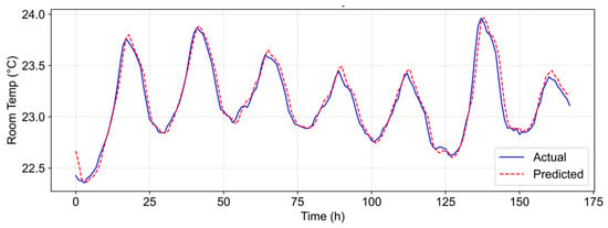
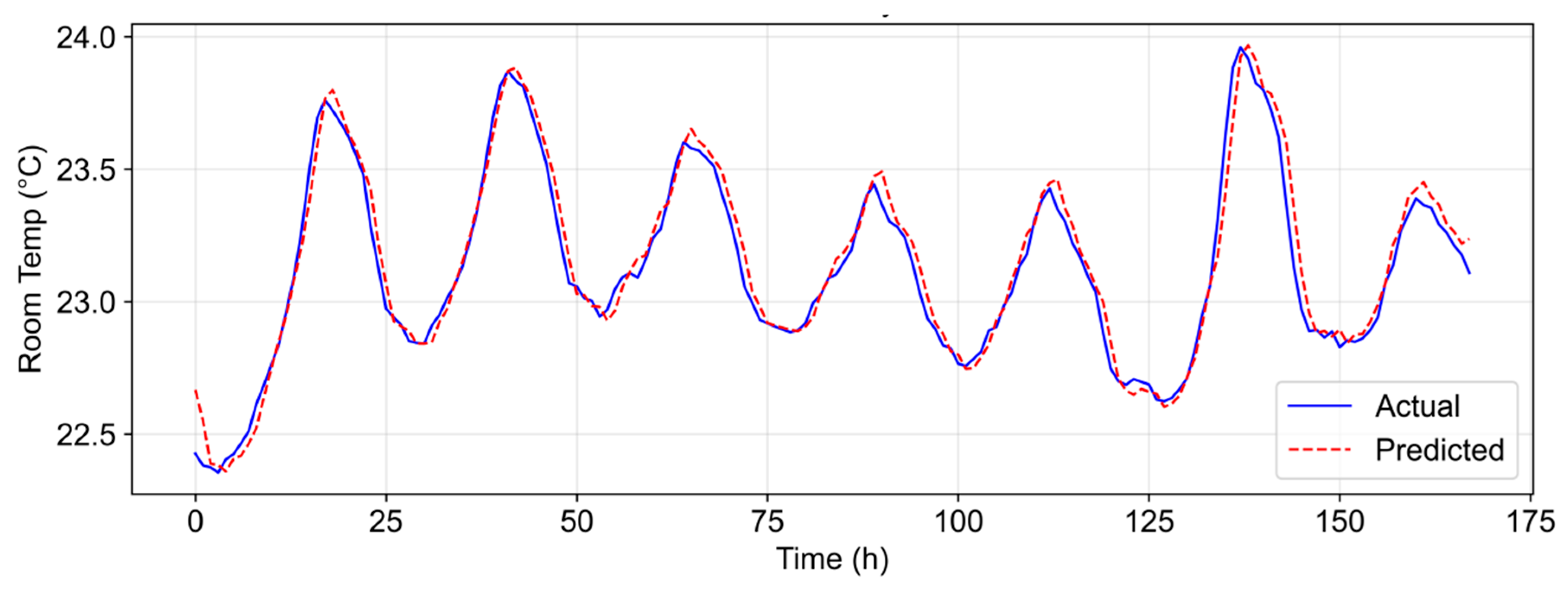
To further verify the long-term stability of the model in continuous multi-day rolling prediction, a typical user with complete data is selected, with 16 December 2024 as the starting point. Data from the 15 days prior to the prediction day are used for training, and continuous prediction is performed for 7 days (168 h). Figure 6 shows the hourly room temperature prediction curve of this user for 7 consecutive days.

Figure 6. Hourly room temperature prediction curve of a typical user for 7 consecutive days.

As shown in Figure 6, the prediction curve is highly consistent with the measured curve in overall trend over the 7 consecutive days. The model can accurately capture the daily day–night temperature fluctuation pattern. Under the hourly innovation correction mechanism of Kalman filtering, the prediction error does not accumulate and amplify with the increase in prediction duration, indicating that the model still has good stability and engineering applicability in long-term rolling prediction scenarios.

5. Rolling Control Framework for Room Temperature Prediction and Engineering Application

5.1. Overview

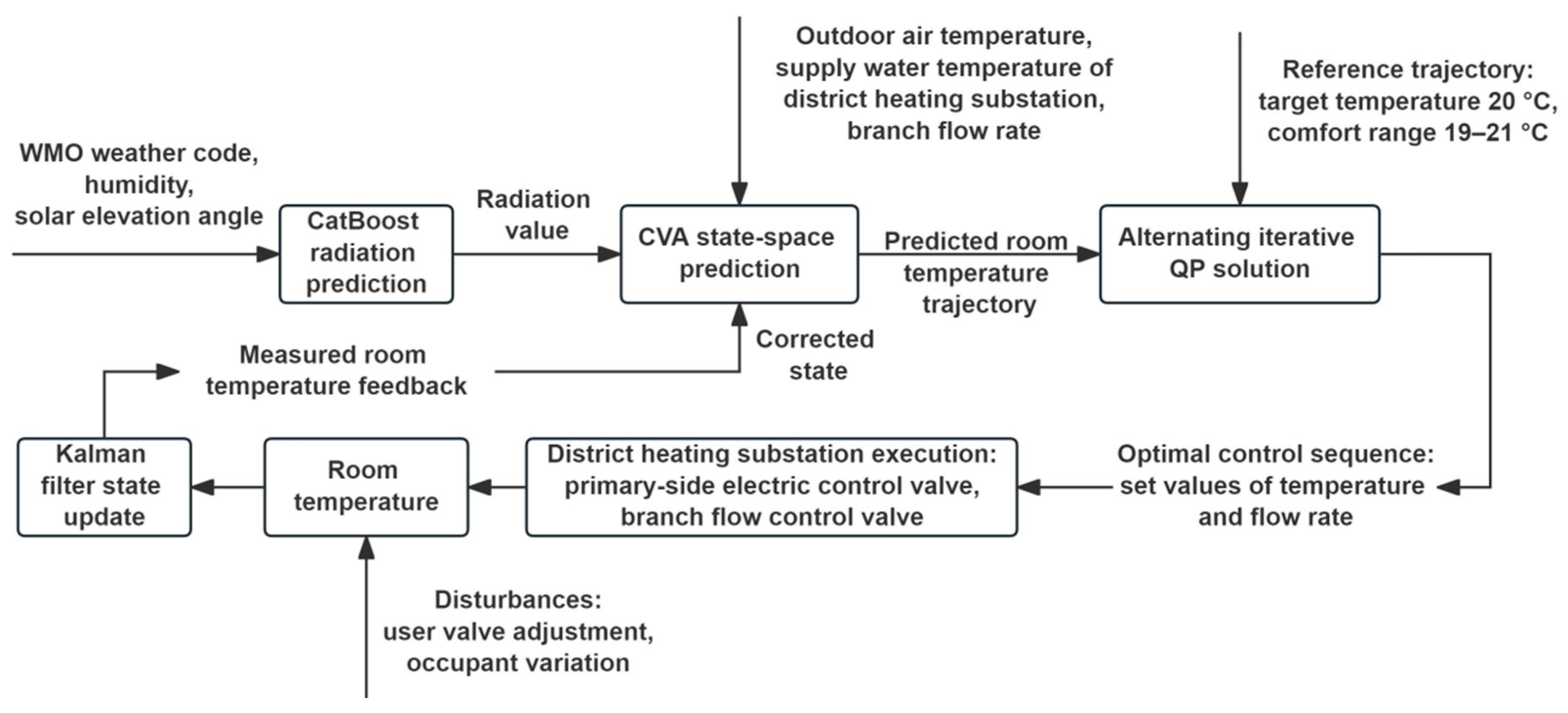
The fundamental value of room temperature prediction lies in shifting heating control from “post-event compensation” to “pre-event prediction.” Traditional outdoor temperature compensation curves adjust the supply water temperature only after the air temperature changes, making it difficult to perceive the synergistic influence of factors such as solar radiation. The control action always lags behind changes in actual heat demand. To overcome this deficiency, this paper introduces the idea of model predictive control on the basis of hourly room temperature prediction and constructs a rolling closed loop of “prediction–optimization–execution–correction.” The controller no longer passively waits for the room temperature to deviate from the target. Instead, based on the corrected state-space model, it performs rolling prediction of the room temperature trajectory over a future horizon and, under the premise of satisfying physical constraints, solves for the optimal control sequence at the current time step. Only the first step of the sequence is executed. At the next time step, the latest measured room temperature feedback is used to correct the state and re-optimize, thereby achieving continuous closed-loop rolling optimization control.

It should be noted that thermostatic valves on the user side can only provide local room temperature control. They operate independently with a relatively slow response and cannot be directly adjusted by the district heating substation. The substation can only regulate the secondary-side supply water temperature and branch flow rates. Therefore, relying solely on local thermostats is insufficient for network-wide coordination, and proactive control based on room temperature prediction at the substation level is needed. The operation logic and closed-loop structure of the entire algorithm are shown in Figure 7.

Figure 7. Flowchart of rolling control for room temperature prediction. The arrows indicate the flow of data, control signals, and feedback in the rolling optimiza-tion process.

5.2. Selection of Representative Users and the Control Scheme

In engineering implementation, it is neither realistic nor necessary to establish an independent control loop for each of hundreds of users. Therefore, this framework adopts the idea of “clustering to select representatives and controlling by cluster.” This paper uses DBSCAN clustering to divide users into four clusters and selects four representative users according to the principle of the closest distance to the cluster center. The DBSCAN parameter settings and clustering process are detailed in reference [34]. Since the dynamic response characteristics of users within the same cluster are highly similar, they will produce similar responses to the same supply water temperature change. Therefore, control decisions only need to be made for a few representative users to cover the entire cluster.

The core objective of control is to make the predicted room temperature trajectory fit the reference trajectory as closely as possible (target temperature T_target = 20 °C, comfort range [19 °C, 21 °C]). Since the secondary side of the district heating substation has only one main supply water pipe, it cannot simultaneously satisfy the differentiated water temperature demands of different users. Moreover, the adjustment of branch flow rates will profoundly change the resistance characteristics of the pipe network and cause hydraulic coupling. If all dimensional decision variables are directly combined and solved, the optimization problem is highly likely to become ill-conditioned and computationally expensive. To this end, this study adopts an alternating iterative quadratic programming solution strategy, decoupling the global decision variables into two subproblems, namely, supply water temperature and branch flow rate, which are solved alternately in a loop. The objective function consists of the squared deviation between the predicted room temperature and the reference trajectory and the penalty term for the control variable adjustment increment. Its specific form is:

$$\underset{\Delta T_c,\Delta f}{\min }{\sum }_{k=1}^{N_p}\left[w_y{\left(y_{t+k|t}-T_{\mathit{target}}\right)}^2+w_T{\left(\Delta T_{c,k}\right)}^2+w_f{\left(\Delta f_k\right)}^2\right]$$

where N_p is the prediction horizon, y_t+k|t is the room temperature prediction value of the CVA model at time t for time t + k, ΔT_c,k and Δf are the single-step adjustment increments of supply water temperature and flow rate, respectively, and w_y, w_T, and w_f are the corresponding weight coefficients. When solving this objective function, physical boundaries and actuator constraints must be strictly satisfied; that is, both the water temperature and flow rate are limited within safe upper and lower bounds, and the single-step adjustment increment must not exceed the maximum step size, so as to avoid the impact of frequent actions on the hydraulic system of the pipe network:

$$\left\{\begin{array}{c}{T}_{c,\min }\le T_c\le T_{c,\max }\\ f_{\min }\le f\le f_{\max }\\ |\Delta T_c|\le \Delta T_{\mathrm{step}},|\Delta f|\le \Delta f_{\mathrm{step}}\end{array}\right.$$

where ΔT_step = 0.5 °C/h, Δf_step = 0.1 m³/h.

In the alternating iterative solution process, first, under the premise of keeping the current branch flow distribution unchanged, based on the room temperature prediction deviation of the main cluster representative user, the optimal adjustment amount of the global unified supply water temperature T_c is solved separately. After the water temperature set value is preliminarily determined, for small-cluster users whose predicted room temperature still deviates from the comfort range, the target branch flow rate f required by each small cluster is back-calculated using the steady-state properties of their CVA models (let (x_t+1 = x_t, y_t = T_target)). At this time, the first group of values in the obtained optimal control sequence is sent to the primary-side electric control valve and the branch flow control valve of the district heating substation for execution. At the next time step, the measured room temperature feedback is used to correct the state in a closed loop and start a new round of optimization, thereby realizing true closed-loop rolling predictive control.

It should be noted that the current optimization formulation treats branch flow rates as independent decision variables and does not explicitly incorporate the full hydraulic network equations. In practice, a simplified strategy of “coarse adjustment of water temperature + fine supplementation of flow rate” is adopted to limit hydraulic disturbance. Water pressure in supply pipes mainly reflects the hydraulic state of the network and is indirectly related to room temperature, so it is currently used only as auxiliary monitoring information. Future work will use resistance identification to address hydraulic coupling and achieve fully joint control of supply water temperature and branch flow rates.

5.3. Simulation Verification and Engineering Deployment

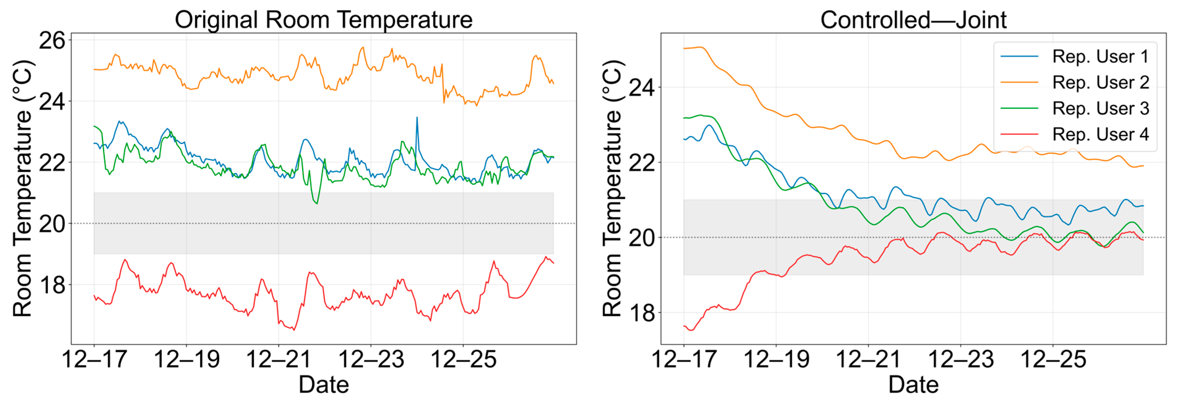
Taking 17 December to 26 December 2024 as the simulation period, data from the 15 days prior to the prediction day are used for model training, and rolling control is performed on the above four representative users. The simulation results are shown in Figure 8. In the simulation, all users share the global supply water temperature back-calculated from the main cluster (representative user 1), and only users with sufficient data excitation (representative users 3 and 4) participate in flow rate fine-tuning. In Figure 7, the controlled room temperatures are generated by the identified CVA state-space models under the proposed rolling control strategy, using historical data from 17 December to 26 December 2024 for simulation, and the results are simulation outputs.

Figure 8. Comparison of room temperatures of representative users before and after control. The dotted line represents the target room temperature (20 °C), and the grey shaded area indicates the comfort range (19–21 °C).

The results show that after an initial transition, the room temperatures of representative users 1, 3, and 4 all converge within the comfort range [19 °C, 21 °C], effectively achieving precise room temperature control. However, for representative user 2 (orange curve), the branch flow rate remains constant during joint control. This is because the standard deviation of the real flow rate in the training window of this user is only 0.05 m³/h, almost in a fixed hydraulic equilibrium state. The lack of sufficient excitation in the data makes it impossible for the model to accurately identify the causal dynamics between flow rate and room temperature. Forcibly back-calculating the control variable could easily cause hydraulic oscillation of the actuator. Therefore, a channel freezing strategy of “passively following the historical real flow rate” is adopted for this user. Because the flow rate of this user does not participate in adjustment, it can only passively accept the globally unique supply water temperature back-calculated from the main cluster. Affected by its own building envelope thermal inertia and hydraulic conditions, the room temperature naturally balances at about 22 °C, slightly higher than the upper limit of the comfort range. This is a safe and slightly warm compromise for individual uncontrollable users under the constraints of ensuring the stability of the global main cluster and preventing pipe network oscillation. From a global perspective, keeping this user in a safe and slightly warm state is far better than significantly reducing the global water temperature in order to force it into the comfort zone, which would cause severe overcooling risk for users in the main cluster. This fully reflects the engineering value of seeking globally optimal decisions under multi-objective constraints.

From the perspective of engineering implementation, the room temperature, supply water temperature, branch flow rate, and weather forecast data required by this framework all come from existing conventional collection systems, without any additional hardware investment. Model training, radiation prediction, and Bayesian filtering parameter tuning are all completed in the offline stage. The online link only involves low-dimensional matrix operations and an alternating iterative quadratic programming solution, with a small computational burden, demonstrating the potential to run on existing PLC controllers in district heating substations. Control instructions can be directly issued to the original actuators without adding additional burden to the existing operation system, and the framework has the engineering deployability to be directly embedded into existing heating control systems.

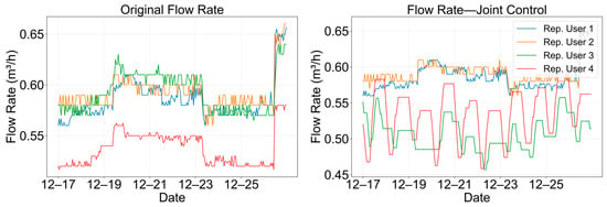
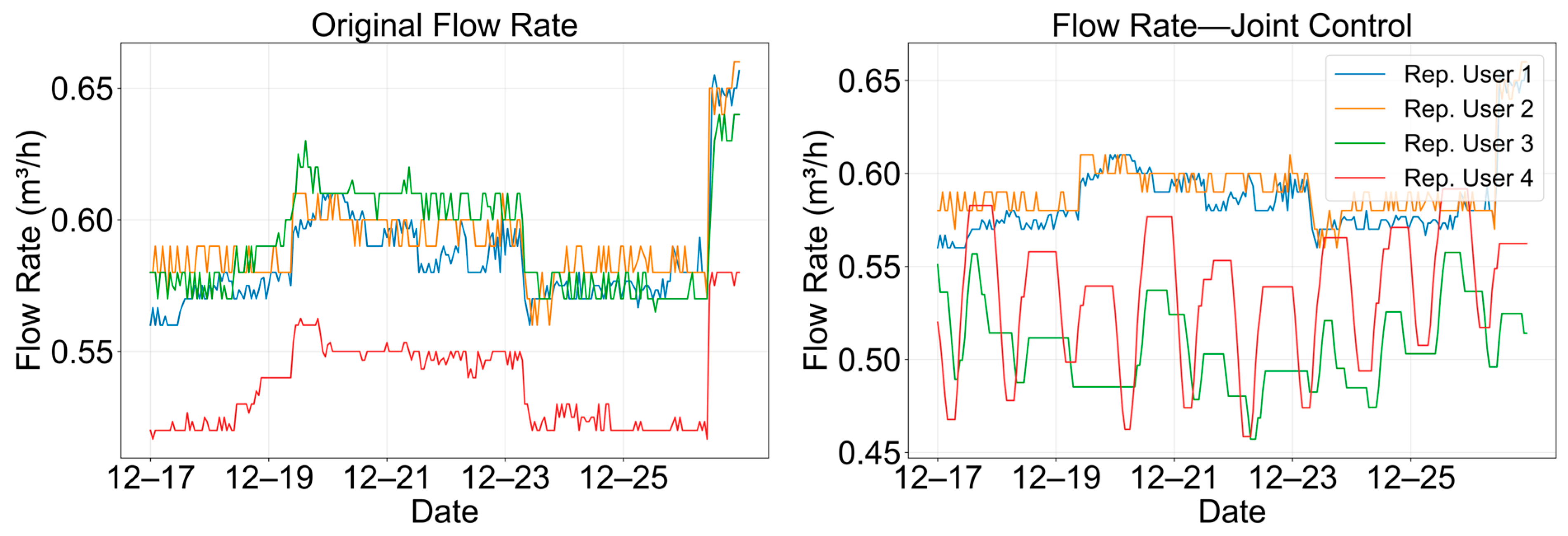
To further illustrate the changes in branch flow rates of each representative user during the control process, Figure 9 presents a comparison of flow rates before and after control. It can be seen that representative users 3 and 4 participate in flow rate fine-tuning, and their branch flow rates change noticeably after control. For representative user 2, since the flow rate variance within the training window is close to zero and the data excitation is insufficient, its historical real flow rate remains unchanged. This result is consistent with the phenomenon shown in Figure 8, where the room temperature of representative user 2 is slightly higher than the upper limit of the comfort range. As the main cluster representative, representative user 1 uses its flow rate for room temperature prediction of the main cluster and back-calculation of the global supply water temperature and does not participate in separate flow rate fine-tuning.

Figure 9. Comparison of branch flow rates of representative users before and after control.

It should be noted that the channel freezing strategy for representative user 2 reflects a systemic limitation of the cluster-based control framework when a user lacks sufficient data excitation. If such a non-excited user is located in a thermally vulnerable unit, passive channel freezing could lead to chronic under-heating rather than slight over-heating. To address this risk, a safeguard mechanism can be introduced in future work: for passive users, their room temperature is continuously monitored, and if it approaches the lower comfort bound, a small controlled excitation signal (e.g., a minor setpoint perturbation) can be applied to safely identify their flow-to-temperature dynamics. Alternatively, the cluster assignment can be adjusted to ensure that vulnerable users are grouped with users who have sufficient excitation.

5.4. Limitations and Prospects

Although the framework shows good prediction accuracy and control potential in real heating season data, it still has certain limitations. The model mainly relies on data from a specific heating season and a specific climate zone for training. If it is transferred to other climate zones or transition seasons, solar radiation contribution patterns and user behavior patterns will change significantly, necessitating recalibration of the model’s applicability. In addition, the verification of the current method is mainly based on offline simulation of historical data. Long-term field closed-loop operation verification on a real district heating substation control loop has not yet been carried out, and the energy-saving rate has not been quantified through field tests. Problems that may exist in actual control systems, such as actuator response lag, communication delay, and controller compatibility, still need to be verified in field engineering. In terms of physical interpretability, although the state variables extracted by CVA subspace identification can correspond to thermal network nodes after similarity transformation, their physical interpretability still needs to be further explored. In the future, deep integration of mechanistic models and data-driven models can be explored. Finally, the current method is suitable for adjustment fine-tuning under slowly time-varying conditions. If extreme conditions such as a large step change in supply water temperature are encountered, online recursive identification or adaptive update strategies will need to be combined to further enhance the robustness of the model against sudden disturbances. Future work will focus on model extension across seasons and multiple climate zones, intelligent recognition of individual behavior, and the construction of a globally optimal framework.

6. Conclusions

Aiming at the problem that terminal room temperature data in district heating systems have not been effectively applied to district heating substation control, this paper proposes a rolling room temperature prediction method that integrates CatBoost solar radiation prediction, CVA subspace identification, and adaptive Kalman filtering. On this basis, a rolling optimization control framework for predictive control of district heating substations is constructed. The verification on 490 valid users in a residential community in Luoyang on 16 December 2024 mainly leads to the following conclusions.

At the level of radiation prediction, the CatBoost model uses conventional weather forecast data to achieve accurate hourly solar radiation prediction, avoiding the deployment requirement of radiation measuring instruments. Through the horizontal comparison of seven methods, under the fair comparison of unified one-hot encoding, CatBoost achieves the best performance with an RMSE of 40.40 W/m². The final model in this paper adopts the native categorical feature processing of CatBoost, and the RMSE is further reduced to 39.26 W/m². Its native processing mechanism for categorical encoding is the key to achieving high accuracy. The feature ablation experiments confirm that the five features, namely, solar elevation angle, WMO weather code, cosine of hour, relative humidity, and sine of hour, all have clear physical meanings and retention values.

At the level of room temperature dynamic modeling, CVA subspace identification can automatically extract a personalized state-space model from the operation data of each user, effectively adapting to significant differences in thermal characteristics among different users without manually presetting the model structure. The hourly correction mechanism of adaptive Kalman filtering is the core for suppressing error accumulation. Bayesian optimization adaptively tunes the filtering parameters for each user. The RMSE of the fixed-parameter scheme is about 15.7% higher than that of the complete method, fully proving the necessity of adaptive tuning. The comparison with typical baseline methods such as ARX, RC network, and LSTM shows that the proposed method achieves the best prediction accuracy under the condition of limited training samples (15 days), verifying the advantages of the “structured model + adaptive filtering” strategy in sample efficiency and engineering practicality. Under six typical weather conditions, the average RMSE for all users does not exceed 0.21 °C, demonstrating good weather robustness.

At the level of control implementation, based on the idea of “clustering to select representatives and controlling by cluster,” this paper adopts an alternating iterative quadratic programming solution strategy to decouple the decision variables and constructs a predictive control framework that includes reference trajectory, physical boundaries, and single-step adjustment amplitude constraints. By cyclically solving the two subproblems of supply water temperature and branch flow rate, closed-loop rolling optimization control of “coarse adjustment of water temperature + fine supplementation of flow rate” is achieved. All data required by this method come from existing conventional collection systems, and the method can run on existing controllers of district heating substations without additional hardware investment, demonstrating its engineering deployability for direct embedding into existing heating control systems. However, the actual energy-saving rate of the proposed control framework still needs to be further quantified through field closed-loop operation.

References

- Li, Z.; Liu, J.; Yang, X.; Huang, X.; Jia, L.; Li, M. Novel effective room temperature-based predictive feedback control method for large-scale district heating substation. Appl. Therm. Eng. 2023, 218, 119241. [Google Scholar] [CrossRef] [Scilit]
- Sun, C.H.; Liu, Y.N.; Cao, S.; Gao, X.; Xia, G.; Qi, C.; Wu, X. Integrated control strategy of district heating system based on load forecasting and indoor temperature measurement. Energy Rep. 2022, 8, 8250–8262. [Google Scholar] [CrossRef] [Scilit]
- Gustafsson, J.; Delsing, J.; van Deventer, J. Improved district heating substation efficiency with a new control strategy. Appl. Energy 2010, 87, 1996–2004. [Google Scholar] [CrossRef] [Scilit]
- Tasic, M.; Ciric, I.; Jovanovic, V.; Ignjatovic, M.; Mitrovic, D. Enhancing thermal comfort in district heating systems through machine learning based estimation and operational control optimisation. Energy Build. 2026, 363, 117580. [Google Scholar] [CrossRef] [Scilit]
- Kalidindi, S.S.V.; Banaee, H.; Karlsson, H.; Loutfi, A. District heating optimization in residential buildings using reinforcement learning with adaptive context-aware predictive environment. Energy AI 2025, 4, 263–279. [Google Scholar] [CrossRef] [Scilit]
- Wang, Y.; Li, Z.; Liu, J.; Pei, M.; Zhao, Y.; Lu, X. Data-driven analysis and prediction of indoor characteristic temperature in district heating systems. Energy 2023, 282, 129023. [Google Scholar] [CrossRef] [Scilit]
- Smertinas, J.; Bacher, P.; Lindström, E. Conditional parametric ARMAX models for observed hourly heat-load dynamics in apartment buildings. Sustain. Cities Soc. 2025, 122, 106235. [Google Scholar] [CrossRef] [Scilit]
- Bergsteinsson, H.G.; Vetter, P.B.; Møller, J.K.; Madsen, H. Estimating temperatures in a district heating network using smart meter data. Energy Convers. Manag. 2022, 270, 116113. [Google Scholar] [CrossRef] [Scilit]
- Gao, C.; Ling, J.; Wang, M.; Yang, Z.; Feng, X. Adaptive transfer learning for household return water temperature prediction based on domain discrepancy metric. Energy 2025, 334, 137692. [Google Scholar] [CrossRef] [Scilit]
- Li, Z.; Liu, J.; Zhang, J.; Wang, Y.; Jia, L. A hybrid control method for district heating substations based on time-based room temperature demand. Energy Build. 2023, 297, 113467. [Google Scholar] [CrossRef] [Scilit]
- Li, Z.; Liu, J.; Jia, L.; Wang, Y.; Zhang, J.; Li, Y.; Cheng, H. Dual room temperature target control of district heating substation based on room temperature detection. Energy Build. 2024, 318, 114430. [Google Scholar] [CrossRef] [Scilit]
- Qian, C.; He, N.; Cheng, Z.; Li, H. An optimal scheduling method for building energy system integrating solar energy based on adaptive hybrid mechanism model and learning-based model predictive control. Energy Build. 2025, 326, 115833. [Google Scholar] [CrossRef] [Scilit]
- Dhaliwal, G.; Gunay, B.; Beausoleil-Morrison, I. Parametric analysis of model predictive control for residential HVAC systems. Energy Build. 2026, 351, 116662. [Google Scholar] [CrossRef] [Scilit]
- Rajagukguk, R.A.; Lee, H. Application of explainable machine learning for estimating direct and diffuse components of solar irradiance. Sci. Rep. 2025, 15, 7402. [Google Scholar] [CrossRef] [Scilit] [PubMed]
- Zerouali, B.; Bailek, N.; Qaysi, S.; Difi, S.; Alarifi, N.; Elbeltagi, A.; Santos, C.A.G.; He, K.; Youssef, Y.M. Hybrid machine learning optimization for solar radiation forecasting. Phys. Chem. Earth Parts A/B/C 2025, 140, 104052. [Google Scholar] [CrossRef] [Scilit]
- Chow, C.W.; Urquhart, B.; Lave, M.; Dominguez, A.; Kleissl, J.; Shields, J.; Washom, B. Intra-hour forecasting with a total sky imager at the UC San Diego solar energy testbed. Sol. Energy 2011, 85, 2881–2893. [Google Scholar] [CrossRef] [Scilit]
- Krishnan, N.; Kumar, K.R.; Sripathi, A.R. Solar radiation forecasting using gradient boosting based ensemble learning model for various climatic zones. Sustain. Energy Grids Netw. 2024, 38, 101312. [Google Scholar] [CrossRef] [Scilit]
- Abdelsalam, H.; Souri, A.; Nan, N. A time series forecasting approach based on gradient boosting method for IoT-based solar energy production systems. Energy Storage Sav. 2025, 4, 413–420. [Google Scholar] [CrossRef] [Scilit]
- Islam, I.; Sristy, S.S.; Jahan, R.; Tareq, M.R.; Hasan, M.; Uddin, P. Advancing solar radiation prediction with explainable AI and ensemble learning techniques. Telemat. Inform. Rep. 2026, 21, 100292. [Google Scholar] [CrossRef] [Scilit]
- Chen, T.; Guestrin, C. XGBoost: A Scalable Tree Boosting System. In Proceedings of the 22nd ACM SIGKDD International Conference on Knowledge Discovery and Data Mining, San Francisco, CA, USA, 13–17 August 2016; pp. 785–794. [Google Scholar] [CrossRef] [Scilit]
- Bacher, P.; Madsen, H. Identifying suitable models for the heat dynamics of buildings. Energy Build. 2011, 43, 1511–1522. [Google Scholar] [CrossRef] [Scilit]
- Jiang, W.; Wang, P.; Ma, X.R.; Liu, Y. Development of a grey-box heat load prediction model by subspace identification method for heating building. Build. Environ. 2025, 280, 113119. [Google Scholar] [CrossRef] [Scilit]
- Toffoli, E. Thermodynamic Identification of Buildings Using Wireless Sensor Networks. In Proceedings of the 17th IFAC World Congress, Seoul, Republic of Korea, 6–11 July 2008. [Google Scholar] [CrossRef] [Scilit]
- Zamani, V.; Abtahi, S.; Li, Y.; Chen, Y. Heating and cooling supply estimation to control buildings temperature using resistor-capacitor thermal model, unscented kalman filter, and nonlinear least square method. Build. Serv. Eng. Res. Technol. 2024, 45, 117–130. [Google Scholar] [CrossRef] [Scilit] [PubMed]
- Van Overschee, P.; De Moor, B. Subspace Identification for Linear Systems: Theory–Implementation–Applications; Springer: New York, NY, USA, 1996. [Google Scholar] [CrossRef] [Scilit]
- Shamachurn, H.; Hassen, S.Z.S. A novel subspace-based framework for the simulative assessment of MPC for HVAC systems in both single and multi-zone buildings. J. Build. Eng. 2026, 124, 115826. [Google Scholar] [CrossRef] [Scilit]
- Ferkl, L.; Siroky, J. Ceiling radiant cooling: Comparison of ARMAX and subspace identification modelling methods. Build. Environ. 2010, 45, 205–212. [Google Scholar] [CrossRef] [Scilit]
- Tang, L.; Xie, H.; Wang, Y.; Xu, Z. Deeply flexible commercial building HVAC system control: A physics-aware deep learning-embedded MPC approach. Appl. Energy 2025, 388, 125631. [Google Scholar] [CrossRef] [Scilit]
- Kalman, R.E. A New Approach To Linear Filtering and Prediction Problems. J. Basic Eng. 1960, 82, 35–45. [Google Scholar] [CrossRef] [Scilit]
- Alam, M.; Rogers, A.; Scott, J.; Ali, K.; Auffenberg, F. Applying extended Kalman filters to adaptive thermal modelling in homes. Adv. Build. Energy Res. 2017, 11, 143–159. [Google Scholar] [CrossRef] [Scilit]
- Fux, S.F.; Ashouri, A.; Benz, M.J.; Guzzella, L. EKF based self-adaptive thermal model for a passive house. Energy Build. 2014, 68, 811–817. [Google Scholar] [CrossRef] [Scilit]
- Wang, S.; Xu, X. Parameter estimation of internal thermal mass of building dynamic models using genetic algorithm. Energy Convers. Manag. 2006, 47, 1927–1941. [Google Scholar] [CrossRef] [Scilit]
- Drgoňa, J.; Arroyo, J.; Figueroa, I.C.; Blum, D.; Arendt, K.; Kim, D.; Ollé, E.P.; Oravec, J.; Wetter, M.; Vrabie, D.L.; et al. All you need to know about model predictive control for buildings. Annu. Rev. Control 2020, 50, 190–232. [Google Scholar] [CrossRef] [Scilit]
- Zhou, E.; Liang, R.; Zuo, T.; Liu, Y.; Du, M. Recognition of Daily Room Temperature Fluctuation Patterns Based on DBSCAN Clustering and Its Dynamic Response Study. Buildings 2026, 16, 3350. [Google Scholar] [CrossRef] [Scilit]
Disclaimer/Publisher’s Note: The statements, opinions and data contained in all publications are solely those of the individual author(s) and contributor(s) and not of MDPI and/or the editor(s). MDPI and/or the editor(s) disclaim responsibility for any injury to people or property resulting from any ideas, methods, instructions or products referred to in the content. |
© 2026 by the authors. Licensee MDPI, Basel, Switzerland. This article is an open access article distributed under the terms and conditions of the Creative Commons Attribution (CC BY) license.