


Abstract
Coastal human settlements concentrate buildings, infrastructure, and populations in climate-sensitive land–sea transition zones, yet maritime proximity does not ensure lower nighttime surface temperatures. Daytime- or hotspot-bassed assessments may therefore miss changes in day–night land surface temperature (LST) contrasts and persistent population co-exposure. This study integrates day–night thermal reorganization, population-weighted LST exceedance, and co-exposure transitions across seven coastal cities in Zhejiang, China. Annual mean daytime and nighttime LST, population, and natural and built-environment covariates were harmonized on 1 km grids for 2012, 2015, 2018, 2021, and 2024. Region-wide associations were evaluated using CatBoost models with SHapley Additive exPlanations (SHAP) and spatial-block validation.. The combined share of relatively high and high nighttime-LST grids was 2.3% in 2012 and 58.2% in 2024, whereas the corresponding daytime share varied across epochs and was 13.8% in 2024. The nighttime contribution to population-weighted LST exceedance was 3.5% in 2012 and 78.2% in 2024. Between 2012 and 2024, 6753 grids entered the high-LST–high-population state, accounting for 54.7% of initially high-population-only grids with valid endpoint data; 1872 grids remained co-exposed in all five epochs. Spatially validated models identified outcome-specific environmental associations. These findings frame coastal urban heat as a reorganization of day–night LST contrasts, population overlap, and state persistence, informing spatial screening for retrofit and preventive planning.
1. Introduction
Climate change and rapid urbanization are transforming extreme heat from a seasonal meteorological hazard into a systemic challenge for urban health and sustainable development. This coupled climate–urban challenge is also emphasized in the latest global synthesis [1]. In 2025, global mean near-surface temperature was approximately 1.43 °C above the 1850–1900 baseline, and 2015–2025 constituted the warmest 11-year period on record [2]. The 2025 Lancet Countdown further estimated that heat-related mortality had increased by 23% relative to the 1990s, reaching approximately 546,000 deaths annually [3]. The challenge is especially salient for China, where the urban population reached 953.8 million and people aged 60 years or older accounted for 23.0% of the population in 2025; the national annual mean temperature was also the highest since 1961 [4,5]. Identifying when and where urban heat intensifies, and how it overlaps with population concentration, is therefore fundamental to climate-responsive planning and equitable adaptation.
China’s coastal zone concentrates the population, economic activity, buildings, and climate-sensitive infrastructure within a limited land area. Along the humid eastern seaboard, monsoonal moisture, prolonged summer heat, and intensive development alter surface energy exchange and can delay nighttime heat release from urbanized surfaces. Zhejiang exemplifies this convergence: its annual mean temperature reached 19.3 °C in 2025, while the province experienced approximately 53 high-temperature days—28 more than the climatological average—and a hot season extending from June to mid-October [6]. The close spatial coupling of climatic exposure, dense settlement, and extensive built-up land makes coastal built environments a critical setting for climate-adaptive planning and retrofit prioritization.
Daytime and nighttime surface temperatures can change differently, altering their spatial contrast and overlap with population. Recent evidence indicates earlier compound-heat onset, expanding the exposure duration, and weakening urban–rural contrasts in nighttime humid heat across China and the Yangtze River Delta [7,8,9]. Epidemiological studies further show that compound daytime–nighttime heatwaves produce larger mortality effects than daytime- or nighttime-only events, with older adults and women showing greater vulnerability [10,11,12,13]. Here, thermal reorganization denotes changes in annual mean daytime and nighttime land surface temperature (LST), their spatial distributions, and their contrast. This regional perspective complements event-based heat assessments.
Recent research on coastal built environments indicates that proximity to the sea does not generate a spatially uniform cooling effect. Hong et al. [14] revealed marked spatial heterogeneity in marine cooling across Xiamen; Bian et al. [15] integrated satellite-derived LST with microclimatic and building-performance indicators in a high-density coastal setting; and Li and Wang [16] showed that the thermal associations of urban form differ among Chinese coastal cities. Further evidence suggests that marine cooling is modulated by prevailing wind conditions, local climate zones, shoreline geometry, and the diurnal cycle, while ocean warming may weaken sea–land-breeze circulation [17,18,19]. Collectively, these studies indicate that coastal thermal patterns reflect the combined influences of marine processes and urban morphology rather than a simple, spatially uniform cooling gradient. Nevertheless, most existing studies examine individual cities, cross-sectional conditions, or specific circulation mechanisms, leaving the multi-epoch reorganization of daytime and nighttime thermal conditions across a multi-city coastal region insufficiently understood.
Research has increasingly moved beyond mapping thermal conditions toward assessing population exposure. Population-weighted and spatially explicit exposure assessments integrate remotely sensed thermal metrics with human-settlement patterns, although their results remain sensitive to spatial scale, exposure definitions, and spatial-linkage methods [20,21,22]. Evidence from China indicates that nighttime heat exposure has increased more rapidly than daytime exposure in many cities [23], while regional assessments identify the Shanghai–Hangzhou Bay corridor as a major concentration of thermal hazard and population exposure [24]. Urban land use may also exert a stronger influence on nighttime than daytime warming and may alter the spatial distribution of heat-related morbidity [25], underscoring the need to link urban thermal evidence with coordinated health and climate action [26]. However, most existing studies quantify the exposure magnitude or map its spatial distribution at individual time points; few track grid-level transitions across multiple epochs to distinguish persistent co-exposure from newly emerging or reduced-LST states.
The associations between coastal thermal conditions and natural and built-environment factors are often nonlinear, scale-dependent, and spatially heterogeneous [27,28,29,30]. Explainable machine learning methods have therefore been increasingly used to characterize complex response patterns and interactions involving topography, ecological infrastructure, development intensity, and urban form. Recent studies further emphasize the importance of spatial lags and geographical variation in these relationships [31,32]. Nevertheless, conventional random training–validation splits may place neighboring observations in both subsets, allowing spatial dependence to inflate apparent predictive performance [33,34]. Spatial-block cross-validation is therefore needed to reduce spatial dependence between training and validation samples and provide a more realistic assessment of regional predictive performance. Moreover, explanatory modeling typically focuses on cross-sectional or individual thermal outcomes and is rarely integrated with multi-epoch exposure-state transitions, leaving the relationships between these transitions and natural and built-environment conditions insufficiently understood.
Taken together, previous studies have provided important evidence on coastal thermal processes, population exposure, and the associated natural and built-environment conditions. However, these three lines of inquiry remain weakly integrated, limiting a process-based understanding of how day–night thermal reorganization reshapes population co-exposure across multiple observation epochs and how the resulting spatial transitions relate to environmental context. Accordingly, this study examines Hangzhou, Jiaxing, Shaoxing, Ningbo, Zhoushan, Taizhou, and Wenzhou—the seven coastal prefecture-level cities of Zhejiang—using a harmonized 1 km grid for 2012, 2015, 2018, 2021, and 2024. Specifically, the analysis investigates (1) the stagewise changes and spatial reorganization of daytime LST, nighttime LST, and their day–night difference; (2) the redistribution of the population-weighted surface overheating index (PSOI) and co-occurrence of relatively high annual mean LST and high population (HH + HP), including persistent, emerging, and reduced-LST transitions; and (3) the nonlinear and interactive associations of the four LST and PSOI outcomes with natural and built-environment conditions under spatially structured validation.
The principal contribution of this study lies not in any individual metric or modeling technique, but in integrating three analytical components within a common regional framework: multi-epoch comparison of daytime and nighttime thermal conditions and coastal PSOI gradients, grid-based tracking of co-exposure transitions, and spatially validated explainable modeling of outcome-specific environmental associations. This integration moves beyond single-period hotspot mapping by distinguishing persistent co-exposure cores, emerging co-exposure areas, and reduced-LST transitions across a multi-city coastal region. The analysis reveals a stagewise, nighttime-dominated thermal reorganization, a pronounced shift in population-weighted LST exceedance toward nighttime, and the coexistence of persistent and emerging co-exposure areas. These findings provide a process-oriented basis for differentiating persistent and emerging co-exposure areas for further assessment and planning. The remainder of the paper is organized as follows: Section 2 describes the study area, data, and analytical methods; Section 3 presents the results; Section 4 discusses the principal findings and planning implications; and Section 5 summarizes the conclusions, limitations, and future research.
2. Materials and Methods
2.1. Research Framework
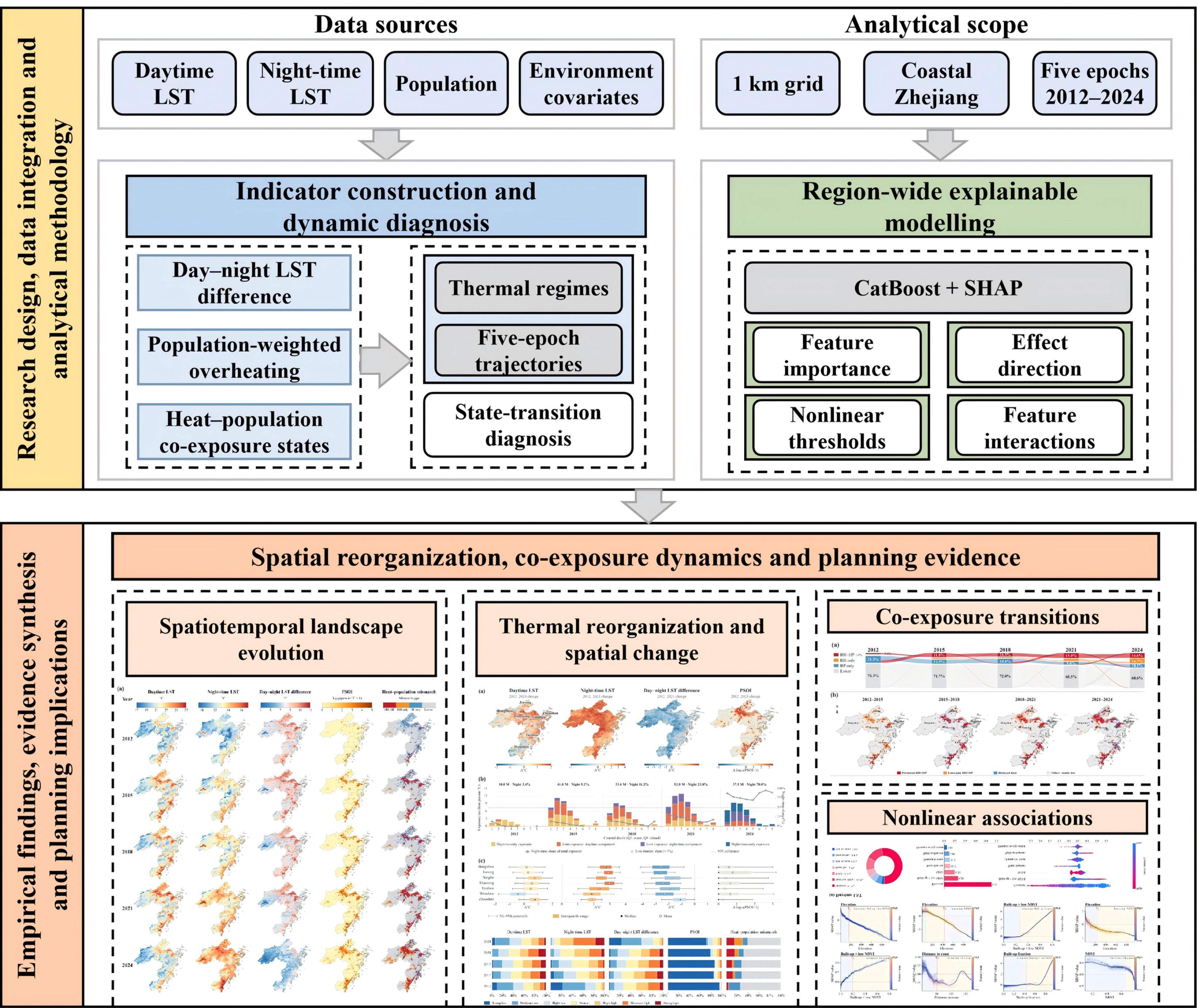
This study follows a progressive logic of thermal characterization, population-weighted LST redistribution, co-exposure transition and explanatory modeling (Figure 1). It connects changes in the physical thermal environment with their implications for established urban settlements, their spatial evolution, and the natural and built-environment conditions associated with those changes.
Figure 1.
Research design, data integration, and analytical workflow. Abbreviations: LST, land surface temperature; SHAP, SHapley Additive exPlanations.
First, daytime LST, nighttime LST and the day–night LST difference characterize stagewise changes in annual mean surface temperature, day–night contrast and spatial coverage across the seven-city coastal region. Second, daytime and nighttime LST exceedances are combined with population distribution to construct PSOI, while coastal-distance groups reveal the redistribution of population-weighted LST exceedance across the settlement system. Third, relatively high annual mean LST and high-population conditions are cross-classified, and adjacent-period transitions, endpoint transitions and five-epoch persistence distinguish established co-exposure cores, emerging co-exposure areas and reduced-LST areas. Fourth, region-wide CatBoost models and SHapley Additive exPlanations (SHAP) importance, dependence and interaction analyses identify nonlinear predictive associations between natural and built-environment factors and the LST and PSOI outcomes.
All analytical stages use a common 1 km spatial unit, fixed classification thresholds and consistent processing rules to ensure comparability across epochs and indicators. Spatial-pattern and state-transition analyses identify where coastal settlements remain exposed, newly cross the co-exposure threshold or fall below the relative LST thresholds, whereas explainable machine learning differentiates the associated natural and built-environment conditions. The five observational snapshots provide the temporal basis for comparing these stagewise patterns.
2.2. Study Area
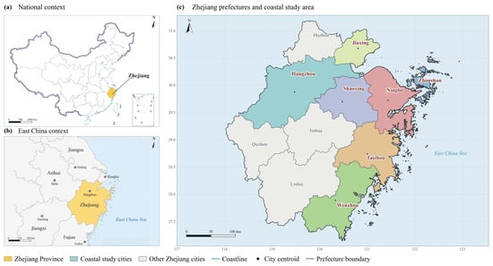
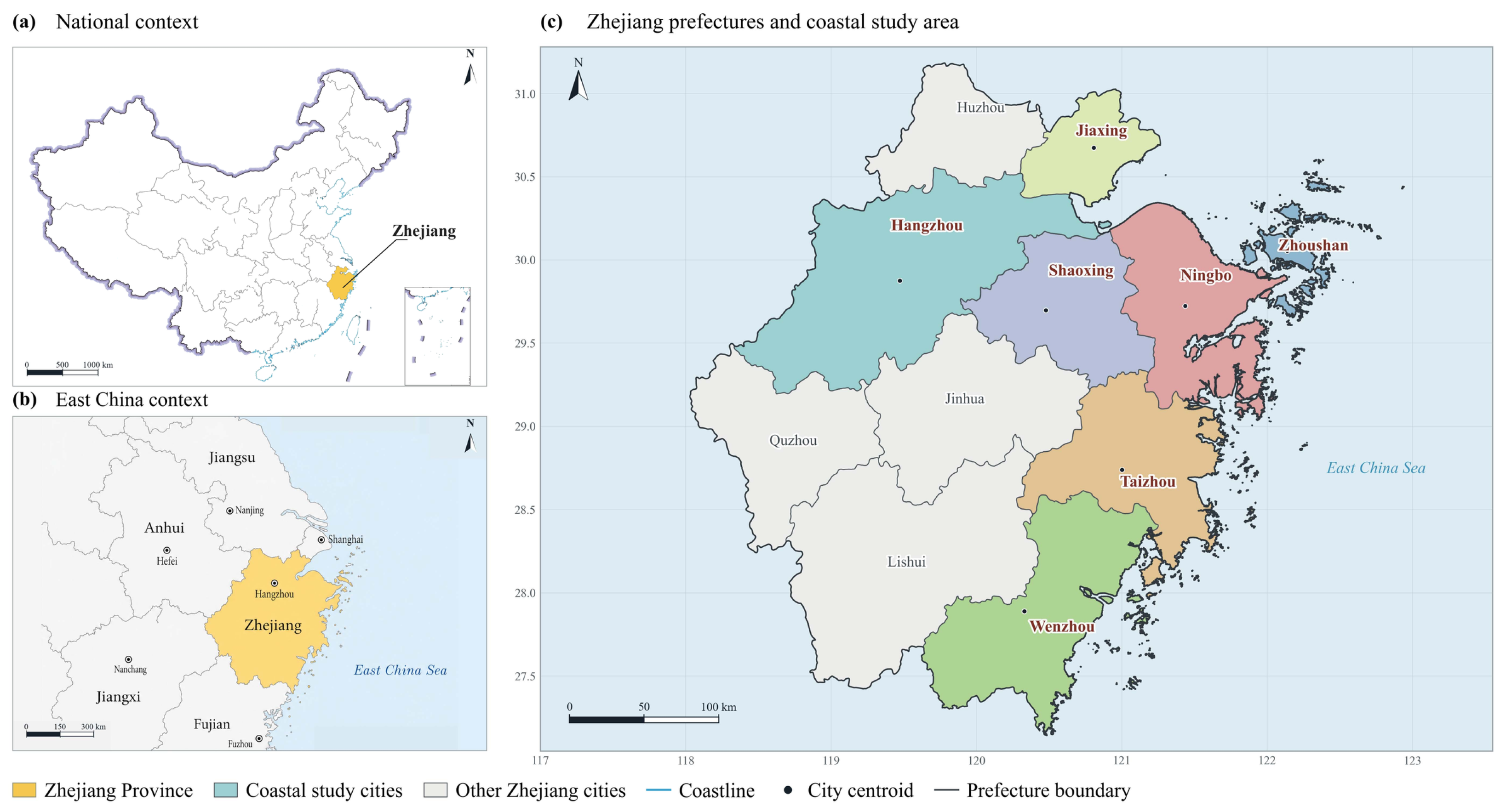
Zhejiang Province lies on China’s southeastern coast and forms the southern wing of the Yangtze River Delta (Figure 2), one of the country’s most urbanized regions. In 2025, the provincial annual mean temperature reached 19.3 °C and the average number of high-temperature days was approximately 53, both markedly above climatological levels [6]. Zhejiang has approximately 6633 km of coastline, including about 1840 km of mainland coastline. Its indented shores, bays and islands create strong land–sea transition conditions around densely developed coastal human settlements [35].
Figure 2.
Regional context of Zhejiang’s coastal human-settlement system. (a) Zhejiang in the national context; (b) Zhejiang in East China; and (c) the seven coastal study cities—Hangzhou, Jiaxing, Shaoxing, Ningbo, Zhoushan, Taizhou and Wenzhou—within the provincial prefecture system.
The study covers the full administrative extents of Hangzhou, Jiaxing, Shaoxing, Ningbo, Zhoushan, Taizhou and Wenzhou, including mountainous and sparsely populated areas as well as built-up land. From north to south, they continuously cover Hangzhou Bay and the Qiantang River estuary, the Ningbo–Shaoxing coast, the Zhoushan archipelago and the southeastern Zhejiang coast, encompassing the province’s principal coastal concentrations of residents, buildings, infrastructure, industry and built-up land. In 2025, the seven cities had a combined permanent population of approximately 51.43 million and a gross regional product of RMB 7.82 trillion, accounting for 76.8% and 82.7% of the provincial totals, respectively [36]. This concentration makes the seven-city system an appropriate regional laboratory for examining surface thermal patterns in rapidly urbanizing coastal human settlements.
Across the seven cities, densely developed coastal plains and estuarine areas adjoin inland mountains, river valleys and islands. This variation in terrain, coastal position and settlement distribution provides a regional basis for comparing day–night thermal patterns and their overlap with population. Examining the cities within a common framework allows persistent and emerging co-exposure areas to be identified across contrasting natural and built environments.
2.3. Data Sources and Preprocessing
2.3.1. Land Surface Temperature Data
Annual daytime and nighttime LST rasters were downloaded from the China Annual 1 km Land Surface Temperature Dataset [37]. The dataset was derived from Moderate Resolution Imaging Spectroradiometer (MODIS) MOD11A2 eight-day composites [38] through monthly averaging followed by annual aggregation. Annual mean LST was selected to compare year-round regional thermal patterns across observation years rather than warm-season extremes. The parent 8-day product provides quality-control (QC) flags, QC_Day and QC_Night for retrieval status, data quality, emissivity error, and LST error [39]. Collection 6 MODIS LST has been evaluated against in situ measurements [40]. Five observation years (2012, 2015, 2018, 2021, and 2024) at three-year intervals supported adjacent-period transition and five-epoch persistence analyses. Annual means represent between-epoch differences, which may reflect interannual meteorological variability, rather than annual trends, continuous warming, or acceleration. Fill and NoData values in the annual rasters were excluded from the analysis. Digital numbers (DN) were converted using the 0.02 K scale factor [39]:
LST (°C) = 0.02 × DN − 273.15
All LST rasters were harmonized to a common coordinate reference system, spatial extent, and 1 km analytical grid, and daytime and nighttime values were extracted at grid centroids. LST summaries used valid observations in each epoch. State summaries used the 59,927-grid classification panel; spatial-extent model sensitivity analyses used a separate complete-case sample (Table A1). LST represents surface radiometric temperature and is not equivalent to near-surface air temperature or human thermal comfort [41]. A supplementary analysis examined Terra observation times and compared the direction of nighttime LST change in independently processed MOD11A2 and Aqua MYD11A2 series (Table A2).
A QC-filtered MOD11A2 Collection 6.1 series was constructed for the five observation years, retaining good-quality retrievals with estimated LST errors ≤ 1 K [38,39]. Annual means were calculated as equal-weight averages of monthly means, requiring valid observations in all twelve months without gap filling. Comparisons used grids with valid annual values in both datasets (Table A3).
2.3.2. Population and Natural–Built-Environment Variables
Population data were obtained from the constrained WorldPop 2020 population-count raster at an approximate resolution of 100 m and aggregated to the total population within each 1 km grid [42,43]. The 2020 population surface was held fixed across all five epochs. Co-exposure transitions therefore describe thermal changes over a common population baseline. Population was used only to construct PSOI and co-exposure states and was not included as an explanatory variable in the machine learning models. The 2025 population statistics were used only to describe the study-area context and did not enter the grid-level analysis.
Natural and built-environment variables included elevation, normalized difference vegetation index (NDVI), built-up fraction, water fraction, distance to the coast and distance to the city center. Elevation was obtained from the Shuttle Radar Topography Mission Global 1 arc-second (SRTMGL1) dataset, version 003 [44]; annual mean NDVI for 2020 from MODIS MOD13Q1 Collection 6.1 [45]; built-up and water fractions from European Space Agency (ESA) WorldCover 2021 [46]; and coastline geometry from the Global Self-consistent, Hierarchical, High-resolution Geography Database (GSHHG), version 2.3.7 [47]. Only NDVI observations with SummaryQA = 0 were retained, and fill and invalid values were excluded. Valid 16-day composites were averaged over 2020 and aggregated to the 1 km grid using area-weighted averaging. Elevation, NDVI and WorldCover 2021 land cover were fixed across epochs; NDVI therefore represents spatial vegetation context. Built-up and water data were converted to area fractions within each 1 km grid. These variables characterize the regional settlement context.
Distance from each grid centroid to the nearest coastline represented the land–sea positional gradient, while the distance to the city center was calculated as the great-circle distance between each grid centroid and the geometric center of valid grids in the corresponding city. A compound variable, built-up fraction × low NDVI, was further constructed, where low NDVI was defined as 1 − NDVI, to represent the concurrence of a higher development intensity and insufficient vegetation. All datasets were harmonized to the 1 km grid and checked for coordinate reference, spatial extent, missing values, and units, producing a grid–year panel dataset. Table 1 summarizes the data sources, spatial resolutions, preprocessing procedures, and analytical roles.
Table 1.
Data sources, spatial resolution and analytical uses.
2.4. Analytical Methods
2.4.1. Thermal Metrics and Spatial Classes
To characterize the coastal thermal environment in terms of annual mean surface temperature and day–night contrast, daytime LST, nighttime LST and their difference were calculated separately. The day–night LST difference (DNTD) for grid i in observation epoch t was defined as
DNTDi,t = LSTday,i,t − LSTnight,i,t
To compare landscape composition across the five epochs, daytime LST, nighttime LST and DNTD were standardized separately using their pooled five-epoch samples:
Zi,t = (Xi,t − μx)/σx
Using fixed z-score boundaries of −1.5, −0.75, −0.25, 0.25, 0.75 and 1.5, each indicator was divided into seven classes: strong low, moderate low, slight low, neutral, slight high, moderate high and strong high. The same pooled mean, standard deviation and class boundaries were applied to all epochs, making changes in class area directly comparable.
2.4.2. Relative LST Thresholds, PSOI, and Co-Exposure States
Relative LST thresholds were determined from the pooled annual means of all valid grids across the five epochs. The primary analysis used the 90th percentiles (P90) of daytime and nighttime LST, equal to 24.063 °C and 14.880 °C, respectively. These thresholds identify relatively high annual mean surface temperatures, not heatwaves, hot nights, or physiological heat stress. The corresponding exceedance magnitudes were defined as
Hday,i,t = max(LSTday,i,t − 24.063, 0)
Hnight,i,t = max(LSTnight,i,t − 14.880, 0)
The population-weighted surface overheating index (PSOI) quantifies population-weighted annual mean LST exceedance above these relative thresholds:
PSOIi,t = Popi × (Hday,i,t + Hnight,i,t)
Here, Popi denotes the population count in a 1 km grid and PSOI is expressed in person·°C. A log10(PSOI+1) transformation was used for mapping to compress the long right tail, whereas modeling retained PSOI in its original unit. PSOI combines relative LST exceedance with population concentration to support regional thermal screening.
A grid was classified as relatively high LST (HH) when either annual mean daytime or nighttime LST reached its corresponding pooled P90 threshold. A high population (HP) was defined by the regional 75th percentile of the fixed population-grid distribution (466.055 persons per grid). For grids with valid LST and population data, four mutually exclusive states were identified: HH + HP (high LST and high population), HH only (high LST only), HP only (high population only), and lower co-exposure. HH + HP was further divided into daytime-only, nighttime-only and combined high-LST states using unchanged thresholds. Grids lacking daytime LST, nighttime LST or population were marked unavailable rather than assigned a co-exposure state (Table A4).
2.4.3. Thermal Reorganization and Coastal Redistribution of Settlement Exposure
The spatial distributions and class compositions of all indicators were first compared across the five epochs. Grid-level net changes in daytime LST, nighttime LST, DNTD and log10(PSOI+1) were calculated as 2024 minus 2012. At the city level, medians and means represented central tendencies, while interquartile ranges and 5th–95th percentile ranges described within-city heterogeneity.
To characterize exposure redistribution along the coastal-distance gradient, unique grids were ranked by coastal distance and assigned to ten fixed equal-count groups (deciles; distance ranges and medians in Table A5). Only Q1–Q8 were displayed; Q9–Q10 together contributed less than 1% of regional PSOI in each epoch and were omitted only from the visualization. Total PSOI, its daytime and nighttime components, and the nighttime share of total PSOI were aggregated within each group.
2.4.4. Co-Exposure State Transitions and Persistent Cores
Adjacent-period transition maps were constructed for 2012–2015, 2015–2018, 2018–2021 and 2021–2024, together with a row-normalized four-state transition matrix for 2012–2024. The probability of transition from state a to state b was defined as
where Nab is the number of grids moving from state a to state b. For each interval, persistent HH + HP denotes HH + HP at both endpoints; emerging HH + HP denotes entry into this state; reduced LST denotes HH to non-HH, irrespective of population; and other transitions comprise the remaining valid cases. Five-epoch persistent cores require HH + HP in all five epochs. Missing endpoint LST or population is classified as unavailable; the transition matrix uses only valid paired observations.
Pab = Nab/ΣbNab
2.4.5. Region-Wide CatBoost Models
Within the integrated coastal settlement system, four CatBoost regression models were fitted separately for daytime LST, nighttime LST, DNTD and raw PSOI [48]:
yi = f(Xi) + εi
Explanatory variables included elevation, distance to the coast, NDVI, water fraction, built-up fraction, distance to the city center, and built-up fraction × low NDVI. Longitude, latitude, normalized year and city dummy variables controlled for broad spatial position, observation epoch and administrative-unit differences. The models characterize spatial associations across the five epochs, with the year accounting for between-epoch differences. Population was excluded to avoid a mechanical association with its role in constructing PSOI, although built-up predictors may still capture population concentration. All models used 900 iterations, a learning rate of 0.035, a tree depth of 6, an L2 regularization coefficient of 5 and random seed 42; training was capped at 50,000 complete grid–epoch observations to limit computational cost. Observations were sampled without replacement using fixed random seeds, without equal quotas by city or year. In cross-validation, sampling was restricted to the training pool; all held-out observations were retained for evaluation.
To assess population-weighting sensitivity, PSOI was compared with unweighted LST exceedance, defined as the sum of positive daytime and nighttime deviations from their respective P90 thresholds. Both models used matched observations, predictors, training samples and spatial-block and leave-one-city-out splits (Table A6). Model fitting and validation were performed in Python 3.11.2 using CatBoost 1.2.10 and scikit-learn 1.9.0. SHAP values and interaction values were computed using CatBoost’s built-in implementation.
2.4.6. SHAP Attribution, Interactions, and Candidate Change Points
SHAP was used to decompose the contribution of each explanatory variable to model predictions [49]:
f(Xi) = φ0 + Σjφij
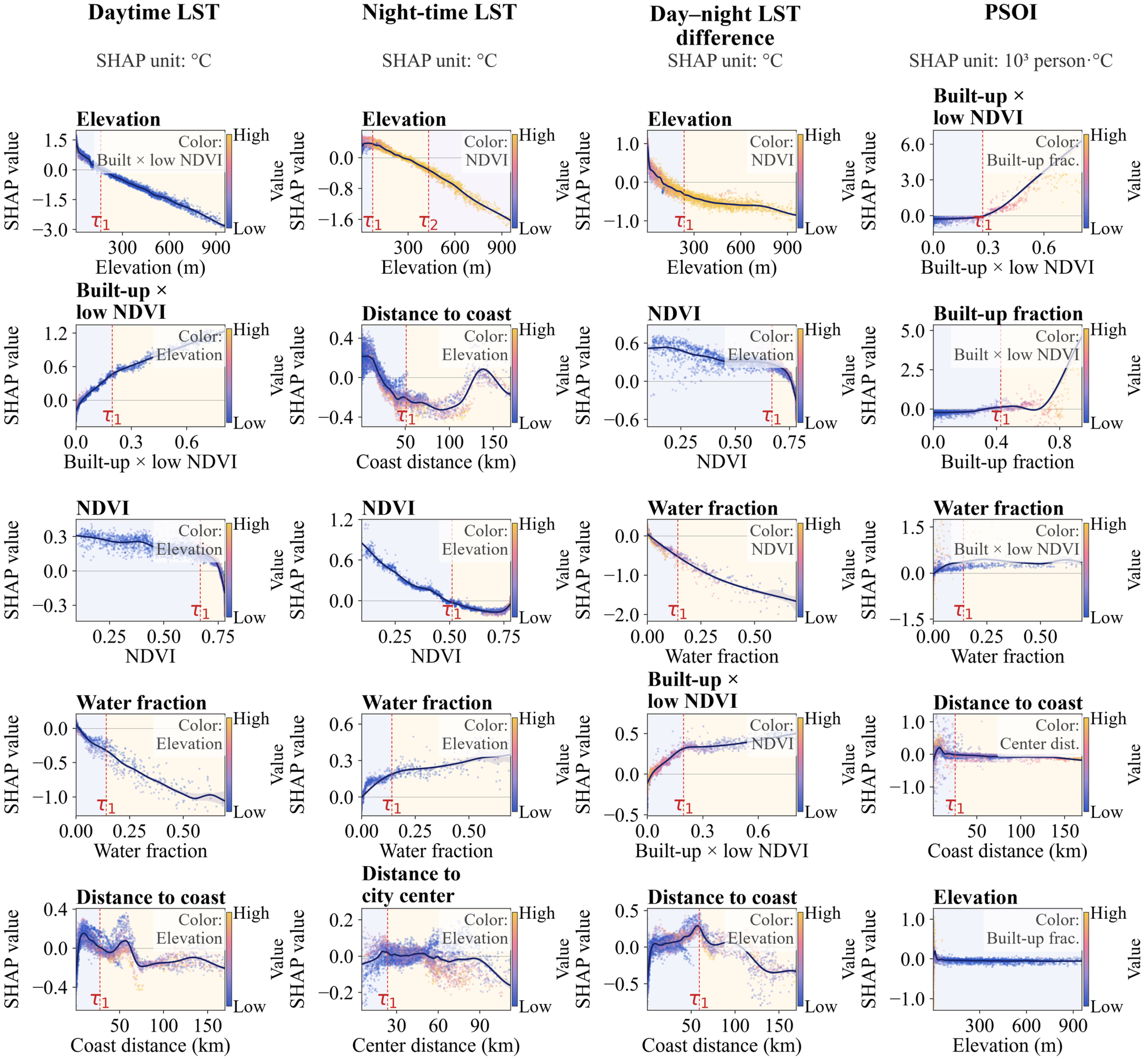
Variable importance was measured by the mean absolute SHAP value, and only the seven mechanism variables were interpreted in the main text. Dependence relationships were plotted for the five leading mechanism variables of each outcome, and the strongest interaction counterpart was identified from SHAP interaction values for 2500 observations. Dependence curves were estimated over the 1st–99th percentile feature range using equal-count bins and smoothing splines. Candidate change points were screened with weighted continuous segmented-linear models and the Bayesian information criterion, and their uncertainty was estimated using 80 bootstrap resamples of feature–SHAP pairs. The 95% percentile intervals were conditional on the fitted model and selected number of change points (Table A7). The retained τ values locate changes in regional predictive associations and identify response ranges for further investigation.
2.4.7. Spatial Validation, Sensitivity Analysis, and Quality Control
The primary generalization assessment used five-fold spatial-block cross-validation. Non-overlapping 25 km × 25 km blocks were constructed from grid coordinates, and observations for the same 1 km grid across all five epochs were assigned to the same fold to reduce information leakage from spatial proximity and repeated observations [33,34]. The 25 km scale was a pragmatic compromise between spatial grouping beyond individual 1 km grids and retaining multiple blocks for five-fold validation. Model performance was evaluated using the coefficient of determination (R2), root mean square error (RMSE) and mean absolute error (MAE). Threshold sensitivity combined relative LST thresholds of P85, P90 and P95 with population thresholds of P70, P75 and P80 to test the stability of HH + HP and the principal transition classes. All cross-epoch analyses used a common grid, fixed thresholds and fixed spatial covariates, with checks of coordinates, units, missing values and grid–year uniqueness. Table A8 reports threshold definitions and 2024 HH + HP occurrence. Table A9 uses all 59,927 study grids as a common denominator and separates mutually exclusive verified endpoint transitions from grids with missing endpoint LST or population. Spatial-extent sensitivity analyses compared the full complete-case sample with built-up subsets using fixed regional thresholds and the same spatial-block validation scheme (Table A1).
3. Results
3.1. Nighttime-Dominated Thermal Reorganization
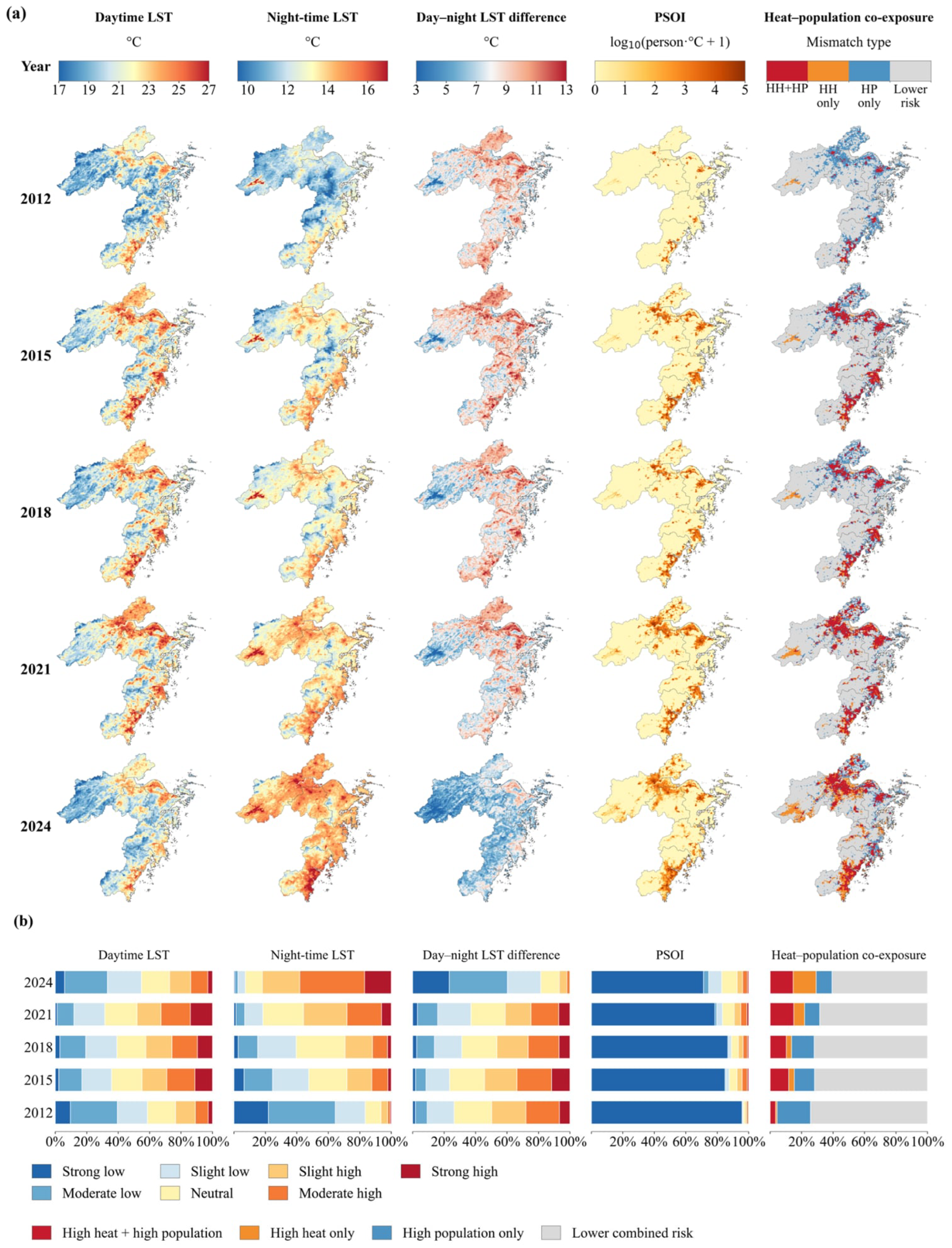
Annual mean daytime and nighttime LST showed divergent patterns across the five observation years. The combined share of grids in the moderate-high and strong-high daytime classes was 11.0% in 2012, 29.1% in 2015, 25.8% in 2018, 32.7% in 2021 and 13.8% in 2024 (Figure 3b). By contrast, the corresponding nighttime share was 2.3% in 2012 and 58.2% in 2024 (Figure 3b), and higher nighttime-LST areas were more spatially extensive in 2024, forming connected settlement belts around Hangzhou Bay, the Ningbo–Shaoxing coast and southeastern Zhejiang (Figure 3a). The five observation years therefore indicate a nighttime-dominated reorganization of the coastal built environment rather than uniform day–night change.
Figure 3.
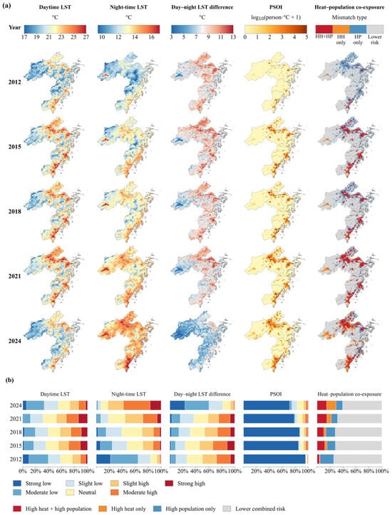
Multi-epoch patterns of surface thermal conditions and LST–population co-exposure across Zhejiang’s coastal human settlements. (a) Spatial distributions of daytime LST, nighttime LST, the day–night LST difference, PSOI, and co-exposure states; (b) indicator-wise landscape composition across five observation years. Abbreviations: HH, relatively high LST; HP, high population; HH + HP, co-occurrence of relatively high LST and high population.
The day–night LST difference was markedly smaller in 2024 than in 2012. The combined share of the strong-low and moderate-low classes was 9.2% in 2012 and 60.2% in 2024, whereas the corresponding share of the moderate-high and strong-high classes was 28.0% and 1.9%, respectively (Figure 3b). The largest between-epoch difference occurred during 2021–2024 (Figure 3a,b), indicating pronounced late-period reorganization. The supplementary Terra and Aqua series also showed higher nighttime LST in 2024 than in 2021 (Table A2). Among common valid grids with complete monthly coverage in both years, the 2021–2024 nighttime LST difference was 0.68 °C in the main dataset and 0.48 °C in the QC-filtered series, indicating a consistent direction of nighttime increase within this subset but sensitivity of its magnitude to quality filtering (Table A3b). Meanwhile, the share of grids with nonzero PSOI was 4.3% in 2012 and 29.3% in 2024 (Figure 3b), with higher PSOI concentrated around Hangzhou Bay, Ningbo and the Wenzhou–Taizhou coastal corridor in 2024 (Figure 3a). By 2024, this redistribution intersected established urban settlements, and many grids previously classified as HP only were classified as areas of high-LST–high-population co-occurrence (Figure 3a).
3.2. Coastal Redistribution of Thermal Change and Nighttime Population-Weighted LST Exceedance
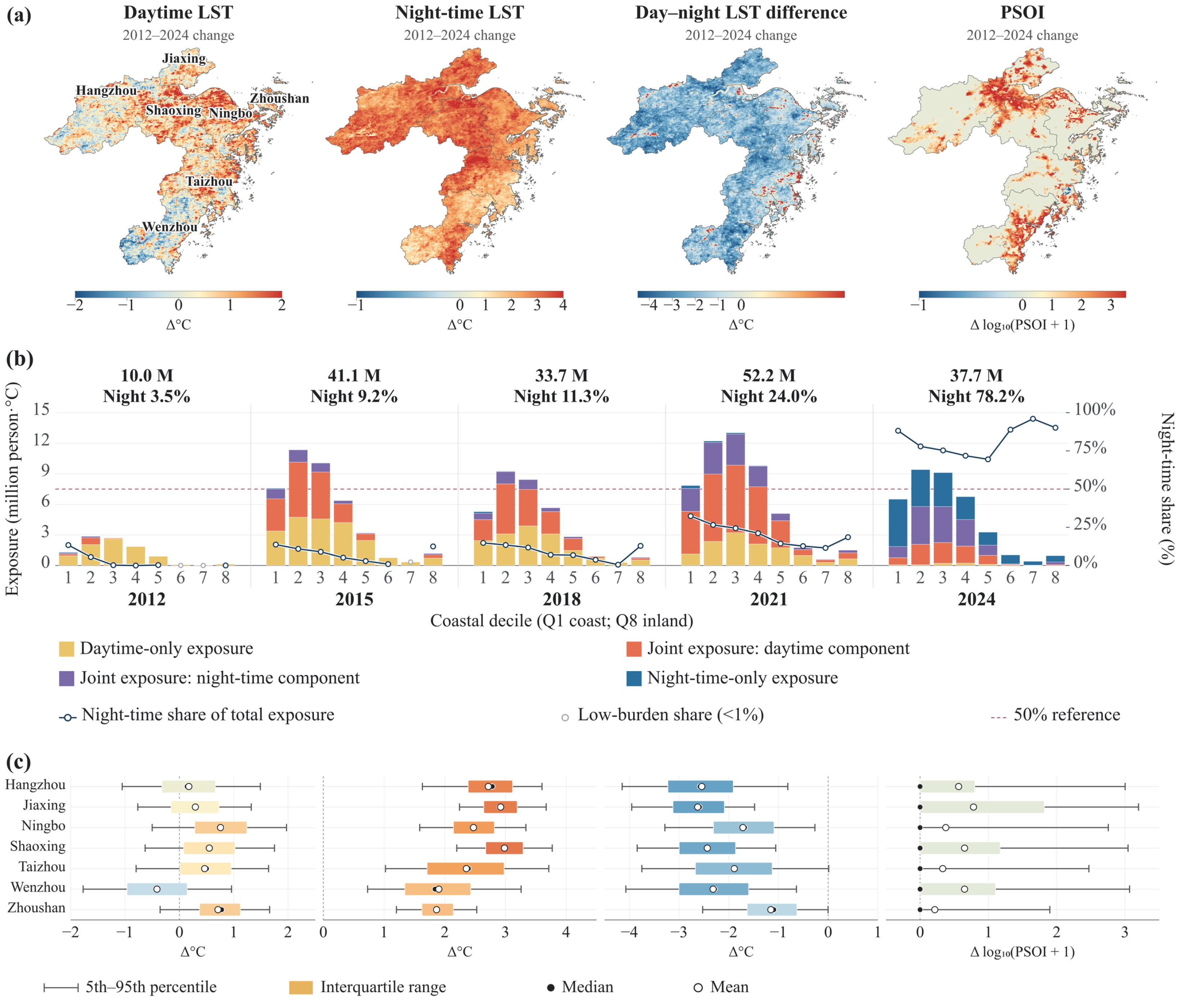
Net-change maps show that nighttime LST was higher in 2024 than in 2012 across most of the study area, whereas daytime differences were spatially mixed and the day–night difference was lower across extensive areas (Figure 4a). Total PSOI was 10.0 million person·°C in 2012, 41.1 million in 2015, reached its highest observed value of 52.2 million in 2021, and was 37.7 million in 2024. Although the total was lower in 2024 than in 2021, the nighttime share was 78.2% in 2024 compared with 3.5% in 2012, indicating a marked difference in the day–night composition of PSOI between the endpoint years.
PSOI was spatially concentrated but compositionally differentiated along the coastal gradient. In 2024, Q1–Q4, extending to 19.34 km from the coast (Table A5), accounted for 84.2% of regional PSOI, and nighttime contributions within these groups ranged from 71.8% to 88.2% (Figure 4b). More inland groups had still higher nighttime fractions (88.9–96.0% in Q6–Q8) but much lower absolute PSOI. Hence, a high nighttime fraction does not necessarily imply a large population-weighted LST exceedance; magnitude, day–night composition and spatial coverage must be interpreted jointly.
City-level distributions further reveal heterogeneous reorganization (Figure 4c). All cities showed positive median nighttime-LST differences between 2012 and 2024, with the largest values in Shaoxing, Jiaxing and Hangzhou. Median daytime-LST differences were negative in Wenzhou and positive in Ningbo and Zhoushan, while the day–night difference was lower in 2024 than in 2012 in every city. PSOI differences were strongly right-skewed, especially in Jiaxing, Shaoxing and Wenzhou, indicating that regional redistribution was shaped by localized PSOI increases rather than uniform citywide change. The full city-by-epoch statistics are provided in Table A10.
Figure 4.
Thermal reorganization and redistribution of population-weighted LST exceedance, 2012–2024. (a) Grid-level net changes; (b) PSOI magnitude and day–night composition across the first eight fixed coastal-distance deciles (Q1–Q8; Table A5); (c) city-level distributions of grid change.
3.3. Persistence and Expansion of LST–Population Co-Exposure
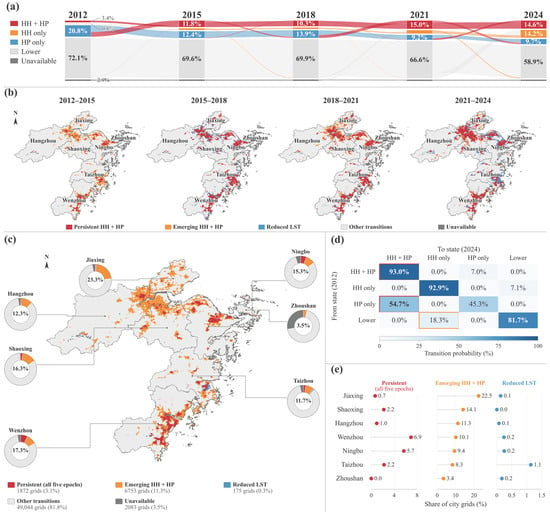
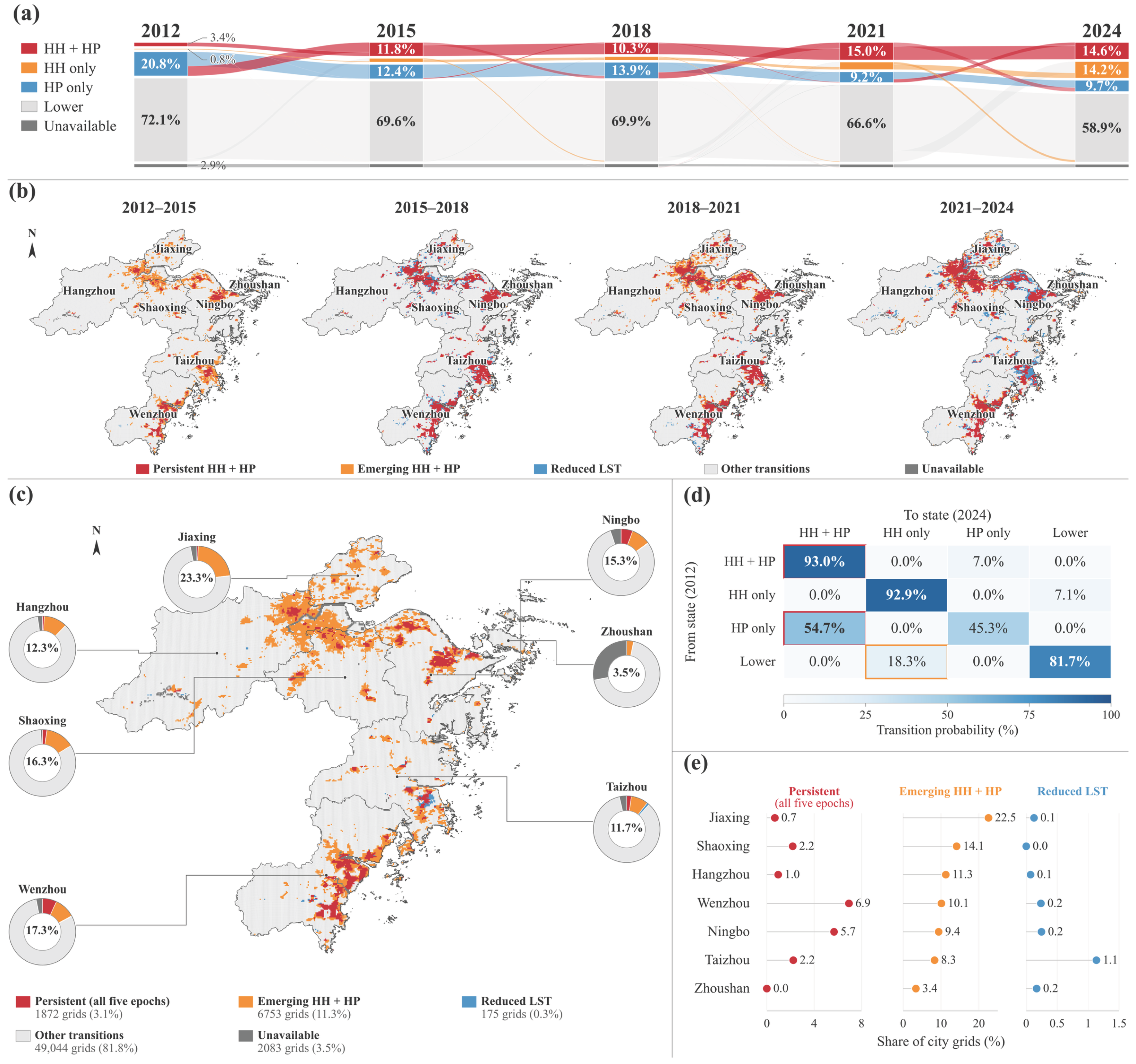
The trajectories show non-monotonic changes in co-exposure extent. HH + HP grids accounted for 3.4% of study grids in 2012, 11.8% in 2015, 10.3% in 2018, 15.0% in 2021 and 14.6% in 2024 (Figure 5a). Adjacent-period maps locate co-exposure expansion around Hangzhou Bay, the Ningbo metropolitan area and the Wenzhou coast, while also revealing localized transitions below the relative LST thresholds (Figure 5b).
Figure 5.
LST–population co-exposure transitions: (a) state trajectories; (b) adjacent-period transitions; (c) five-epoch persistent cores and 2012–2024 emerging/reduced-LST transitions; (d) endpoint transition matrix, with red outlines indicating HH + HP persistence and transitions from HP only to HH + HP, and an orange outline indicating transitions from Lower to HH only; and (e) city shares corresponding to (c). Donut centers sum persistent, emerging and reduced-LST shares.
The 2012–2024 transition matrix indicates strong endpoint persistence and a dominant conversion pathway (Figure 5d). Among grids with valid endpoint LST and population data, 93.0% of those classified as HH + HP in 2012 remained HH + HP in 2024, while 54.7% of initially HP-only grids transitioned to HH + HP.
A total of 1872 grids remained HH + HP in all five epochs, representing 3.1% of study grids and defining five-epoch persistent co-exposure cores (Figure 5c). Between 2012 and 2024, 6753 grids entered HH + HP (11.3% of study grids), while 175 shifted from HH to non-HH (0.3%; Table A4 and Table A9). Emerging shares were highest in Jiaxing, followed by Shaoxing and Hangzhou, whereas five-epoch persistent shares were highest in Wenzhou and Ningbo (Figure 5e). Distinguishing persistent from emerging co-exposure areas provides a temporal basis for spatial screening and planning that a single-year hotspot map cannot provide. Across all nine threshold combinations, emerging HH + HP remained more extensive than endpoint-persistent HH + HP, although their absolute shares varied (Table A8 and Table A9).
Among the 6753 verified emerging HH + HP grids between 2012 and 2024, 85.9% were nighttime-only, 9.3% exceeded both thresholds and 4.7% were daytime-only in 2024 (Table A4). All 1746 new HH + HP grids between 2021 and 2024 were nighttime-only, whereas daytime-only states predominated among new entries in the earlier intervals. Thus, the nighttime predominance is clearest in the endpoint comparison and the latest interval, rather than across every interval.
3.4. Spatially Validated Natural and Built-Environment Associations
Spatial-block validation produced median R2 values of 0.840 for daytime LST, 0.830 for nighttime LST, 0.777 for the day–night difference and 0.419 for PSOI (Table 2). Thus, the temperature models retained good within-region predictive performance after spatially neighboring and repeated observations were separated between training and validation sets, whereas PSOI was more difficult to predict. In the paired comparison, PSOI performance was weak under city-holdout validation (median R2 = 0.173), with substantial overprediction in Zhoushan (Table A6). Random-holdout and city-holdout diagnostics for the main models are reported in Table A11.
Table 2.
Five-fold 25 km spatial-block cross-validation.
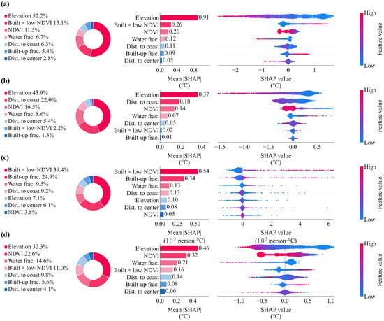
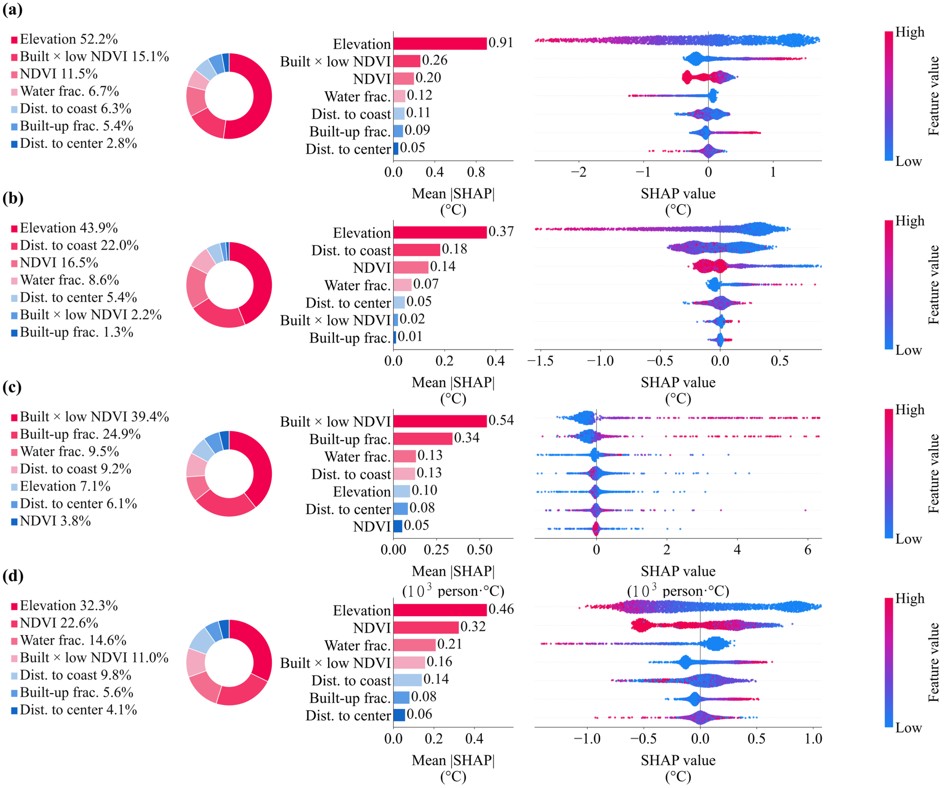
The SHAP rankings differed markedly among outcomes (Figure 6). In the full regional models, elevation dominated daytime LST (52.2%; mean |SHAP| = 0.91 °C), nighttime LST (43.9%; 0.37 °C) and the day–night difference (32.3%; 0.46 °C). Daytime LST was additionally associated with built-up × low NDVI and NDVI, whereas nighttime LST showed a stronger contribution from coastal distance and NDVI. For PSOI, the built-up × low NDVI (39.4%) and built-up fraction (24.9%) together accounted for 64.3% of displayed importance. Sensitivity analysis showed that elevation importance declined within built-up areas, particularly for nighttime LST, suggesting that its regional dominance partly reflects mountain–plain contrasts (Table A1). In the paired comparison, the combined held-out SHAP share of built-up fraction and built-up × low NDVI decreased from 59.5% for PSOI to 27.3% for unweighted LST exceedance (Table A6). Removing the constructed interaction had little effect on thermal-model performance but altered the relative SHAP contributions of built-up fraction and NDVI in the PSOI model (Table A12).
Figure 6.
Global SHAP importance and effect direction for the four outcome models: (a) daytime LST; (b) nighttime LST; (c) PSOI; and (d) day–night LST difference. Donut and bar charts show relative and absolute mean |SHAP| values; beeswarm plots show effect direction, with color indicating feature value. PSOI is expressed in 103 person·°C. SHAP values indicate predictive associations rather than causal effects. Abbreviations: Dist., distance; frac., fraction.
3.5. Regional Nonlinear Associations and Key Interactions
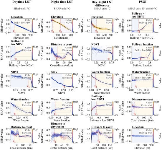
Full-region SHAP dependence curves revealed outcome-specific changes in predictive response (Figure 7). Daytime LST responses changed near 160 m elevation, 0.196 built-up × low NDVI, 0.667 NDVI, 0.141 water fraction and 27.4 km from the coast. Nighttime LST showed elevation changes near 71 and 430 m and a coastal-distance change near 51.0 km; NDVI and water-fraction changes occurred near 0.511 and 0.141, respectively, but with opposing directions. The recurring water-fraction point highlights day–night asymmetry rather than a universal cooling effect.
Figure 7.
Nonlinear SHAP dependence, retained candidate change points and primary interactions for the four outcomes. Curves show smoothed dependence for the five leading predictors; point color denotes the strongest interacting feature. Red dashed lines mark retained change points.
Exploratory PSOI responses changed near 0.268 built-up × low NDVI, 0.426 built-up fraction, 0.141 water fraction and 25.1 km coastal distance. Candidate changes for the day–night difference occurred near 237 m elevation, 0.667 NDVI, 0.141 water fraction, 0.196 built-up × low NDVI and 59.1 km coastal distance. Conditional 95% intervals for the reported change points are provided in Table A7. These regional associations do not establish causal thresholds, but provide reference ranges for local thermal assessment and planning-oriented investigation.
4. Discussion
4.1. Nighttime Thermal Reorganization in Coastal Built Environments
The principal finding is a stagewise divergence between annual mean daytime and nighttime LST, with the observed reorganization dominated by higher nighttime LST. City-level annual mean nighttime LST was 1.86–2.98 °C higher in 2024 than in 2012 (Table A10). Huo and Sun [50] likewise identified diurnal asymmetry in Yunnan during 2001–2020, reporting a nighttime LST trend of 0.43 °C per decade compared with −0.08 °C per decade during the day. Despite differences in observation periods, climatic settings and temporal sampling, both studies identify contrasting daytime and nighttime changes. Here, the smaller day–night LST difference in 2024 captures a shift in annual surface-temperature contrast; its magnitude represents a between-epoch difference rather than an annual trend. Hurduc et al. [51] also demonstrated that surface urban heat-island estimates depend on the season, time of day, and the rural reference, emphasizing the need to distinguish annual LST differences from event-scale or urban–rural thermal metrics.
The non-monotonic coastal-distance responses also differ from a simple coast-to-inland cooling gradient. Hong et al. [14] estimated an average marine influence range of 7.94 km in Xiamen using Landsat-derived LST and 500 m grids. By comparison, our regional SHAP curves identified candidate coastal-distance changes near 27.4 km for daytime LST and 51.0 km for nighttime LST. These values describe changes in conditional predictive associations, not marine cooling limits or sea-breeze penetration distances. The broader spatial support, annual averaging and inclusion of mountain–plain transitions across seven cities help explain the larger response distances. The regional patterns thus highlight the joint relevance of the coastal position, terrain and land-cover configuration for thermal assessment.
4.2. Nighttime PSOI Redistribution and Planning Implications
Thermal reorganization altered both PSOI magnitude and its day–night composition. Total PSOI was highest in 2021 and lower in 2024, whereas nighttime remained the dominant contribution in 2024. The lower 2024 total did not restore the earlier composition; instead, the nighttime component of annual mean LST exceedance remained dominant. For coastal human settlements, this distinction is important because the daytime hotspot extent or mean temperature alone cannot represent the spatial overlap between relative LST exceedance and population concentrations [52,53,54].
Coastal-distance groups further separate PSOI magnitude from composition. Nearer groups contained most of the total PSOI, whereas several inland groups had very high nighttime fractions but small totals. Built-environment screening should therefore combine magnitude, nighttime share and spatial coverage rather than prioritize areas from a single indicator. Because one population surface was held fixed, PSOI changes mainly represent thermal redistribution over an established settlement pattern. PSOI complements assessments of physiologically relevant heat stress by locating surface-temperature and population overlap, which may have different spatial patterns and drivers [55].
4.3. Persistent Co-Exposure Cores and Emerging Planning Priorities
State transitions show that co-exposure expansion combined the persistence of established settlement cores with relative annual mean LST threshold crossing in areas exceeding the regional population threshold. The conversion of HP-only grids to HH + HP provides stronger process evidence than a single-year hotspot map: the population surface was held fixed while the annual mean LST classification changed. These transitions identify changes in thermal conditions within established population concentrations and help prioritize local assessment.
Persistent and emerging grids identify different priorities for further thermal assessment. Persistent cores warrant assessment of existing settlement environments, whereas emerging co-exposure areas warrant preventive assessment where the relative LST threshold has newly been exceeded. Co-exposure expansion around Hangzhou Bay and the coexistence of persistence and emergence in Ningbo and Wenzhou support differentiated regional priorities rather than uniform citywide targets. Linking these spatial priorities with meteorological conditions, vulnerability and adaptive capacity can support subsequent health-oriented assessment [56]. Literature-supported options for these priority areas include external shading and ventilation optimization [57], and reflective or vegetated roofs [58]. These literature-supported measures can be evaluated in the identified priority areas according to local climate and building conditions.
4.4. Built-Environment Associations and Climate-Adaptive Planning Implications
The regional models reveal distinct predictive structures for thermal conditions and population-weighted LST exceedance. Elevation dominated the full-region temperature models, while its reduced importance in built-up subsets highlights the influence of spatial context (Table A1). The built-up × low NDVI and built-up fraction remained the leading PSOI predictors, but their importance was sensitive to population weighting (Table A6). Mo et al. [59] found stronger summer associations between building-land morphology and LST at the block level than at the grid level in Ziyang, with weaker associations in winter. Their season-specific 2D/3D analysis describes the local spatial configuration, complementing the broader context represented by our annual 1 km analysis. Differences in spatial aggregation, predictor definition, and the inclusion of mountainous land therefore help explain why regional elevation dominance can coexist with strong urban-morphology associations in local studies. The present results place local urban-morphology relationships within this wider regional environmental context.
Vegetation associations likewise require attention to the temporal definition and method. Cheng et al. [60] estimated stronger daytime than nighttime cooling from vegetation greening across China during 2000–2018 (−0.36 versus −0.07 K), using a space-for-time approach. Our distinct day–night NDVI responses likewise indicate that vegetation–temperature associations vary over the diurnal cycle. The fixed NDVI layer describes the spatial vegetation context, so the results complement, rather than quantify, the effects of greening over time. Together, the spatially validated temperature models and their nonlinear response ranges help identify environmental conditions for local investigation. In Zhoushan, widespread overprediction of predominantly zero PSOI values produced an extreme negative R2; the unweighted model also performed poorly. These results support using the PSOI model to explore associations within the study region, rather than to predict conditions in cities not represented in training. This regional evidence can guide the selection of priority areas for finer-scale assessment and locally appropriate interventions.
5. Conclusions
This study shows that differences among the five observation years across Zhejiang’s coastal human settlements were characterized primarily by nighttime-dominated thermal reorganization rather than uniform day–night change. Higher nighttime-LST classes occupied a larger spatial share in later observation years, the day–night LST difference was smaller in 2024 than in 2012, and the nighttime contribution to population-weighted LST exceedance was markedly larger in 2024. Co-exposure patterns combined persistent HH + HP grid cores with the transition of baseline high-population grids into relatively high annual mean LST states, identifying persistent and emerging areas for further thermal assessment.
The findings support spatial screening for climate-adaptive planning in coastal built environments. Persistent and emerging co-exposure areas provide priorities for local assessment of retrofit and preventive options, respectively. Spatially validated models identify the environmental context of LST and PSOI patterns, providing a basis for targeted warm-season and site-specific assessment.
This study has several limitations. The five annual LST snapshots and fixed population, land-cover and NDVI layers do not resolve annual trends or changes in settlement and vegetation. Annual averaging also prevents the separation of summer nighttime warming from winter and transitional-season contributions. Meteorological variability and Terra observation-time shifts introduce uncertainty in temporal interpretation, while preprocessing differences limit quantitative comparison between the main annual LST dataset and the independently processed Terra and Aqua LST series reported in Appendix A (Table A2). Without meteorological controls, the models characterize spatial associations rather than causes of thermal change. The 1 km annual-mean framework represents regional surface-temperature and population overlap, not building-scale thermal processes or event-based and physiological heat exposure. Future research should integrate warm-season and upper-tail temperatures, time-varying settlement data, and meteorological and health indicators. Neighborhood simulations and building-level measurements could then evaluate locally appropriate interventions in the priority areas identified here.
Author Contributions
Conceptualization, Y.W. and Y.Q.; methodology, M.Z. and R.Z.; software, M.Z. and R.Z.; validation, Y.W. and C.Z.; formal analysis, M.Z. and C.Z.; investigation, J.M.; resources, Y.Q.; data curation, C.Z. and J.M.; writing—original draft preparation, Y.W. and R.Z.; writing—review and editing, Y.W., M.Z., R.Z. and Y.Q.; visualization, M.Z. and Y.Q.; supervision, Y.W.; project administration, Y.W.; funding acquisition, Y.W. and Y.Q. All authors have read and agreed to the published version of the manuscript.
Funding
This research was funded by the National Natural Science Foundation of China, grant number 52508091.
Data Availability Statement
The underlying datasets are publicly available from the sources cited in the manuscript.
Acknowledgments
During the preparation of this manuscript, the authors used GPT-6 (OpenAI) for language editing, analysis-code assistance and manuscript revision. The authors have reviewed and edited the output and take full responsibility for the content of this publication. We thank the anonymous reviewers for their constructive comments and valuable suggestions, which helped improve the manuscript.
Conflicts of Interest
The authors declare no conflicts of interest. The funders had no role in the design of this study; in the collection, analyses, or interpretation of data; in the writing of the manuscript; or in the decision to publish the results.
Abbreviations
The following abbreviations are used in this manuscript:
| DN | Digital number |
| DNTD | Day–night land surface temperature difference |
| ESA | European Space Agency |
| GAUL | Global Administrative Unit Layers |
| GSHHG | Global Self-consistent, Hierarchical, High-resolution Geography Database |
| HH | Relatively high land surface temperature |
| HP | High population |
| HH + HP | Relatively high LST and high population co-occurrence |
| LOCO | Leave-one-city-out validation |
| LST | Land surface temperature |
| MAE | Mean absolute error |
| MODIS | Moderate Resolution Imaging Spectroradiometer |
| NDVI | Normalized difference vegetation index |
| PSOI | Population-weighted surface overheating index |
| QC | Quality control |
| R2 | Coefficient of determination |
| RMSE | Root mean square error |
| SHAP | SHapley Additive exPlanations |
| SRTMGL1 | Shuttle Radar Topography Mission Global 1 arc-second |
| P70/P75/P80/P85/P90/P95 | 70th/75th/80th/85th/90th/95th percentile |
Appendix A. Supplementary Analyses and City-Level Statistics
Table A1.
Spatial-extent sensitivity under fixed regional thresholds.
Table A2.
Supplementary MODIS processing: regional mean observation times and nighttime LST.
Table A3.
QC-filtered MOD11A2 comparison with the main annual LST dataset.
Table A4.
Daytime and nighttime composition of HH + HP and verified new entries.
Table A5.
Observed distances to the coast within the fixed regional deciles.
Table A6.
Paired comparison of PSOI and unweighted LST exceedance.
Table A7.
Conditional uncertainty intervals for the change points reported in Section 3.5.
Table A8.
Threshold definitions and 2024 HH + HP occurrence. LST thresholds are rounded for display; calculations used full precision.
Table A9.
Verified 2012–2024 endpoint transition composition under alternative thresholds (% of all study grids).
Table A10.
Surface thermal conditions, PSOI, and HH + HP grid shares across seven cities and five observation years. LST means are calculated from the main annual-raster dataset sampled to valid study grids.
Table A11.
Secondary predictive-performance checks for the four CatBoost outcome models.
Table A12.
Sensitivity to removal of the built-up fraction × (1 − NDVI) interaction.
References
- Intergovernmental Panel on Climate Change (IPCC). Climate Change 2023: Synthesis Report; IPCC: Geneva, Switzerland, 2023. [Google Scholar] [CrossRef] [Scilit]
- World Meteorological Organization. State of the Global Climate 2025. Available online: https://wmo.int/publication-series/state-of-global-climate/state-of-global-climate-2025 (accessed on 16 August 2026).
- Romanello, M.; Walawender, M.; Hsu, S.-C.; Moskeland, A.; Palmeiro-Silva, Y.; Scamman, D.; Smallcombe, J.W.; Abdullah, S.; Ades, M.; Al-Maruf, A.; et al. The 2025 report of the Lancet Countdown on health and climate change: Climate change action offers a lifeline. Lancet 2025, 406, 2804–2857. [Google Scholar] [CrossRef] [Scilit] [PubMed]
- National Bureau of Statistics of China. Statistical Communiqué of the People’s Republic of China on the 2025 National Economic and Social Development. Available online: https://www.stats.gov.cn/english/PressRelease/202602/t20260228_1962661.html (accessed on 16 August 2026).
- China Meteorological Administration. China Climate Bulletin 2025; National Climate Center: Beijing, China, 2026. [Google Scholar]
- Zhejiang Climate Center. Climate Monitoring and Assessment of Zhejiang Province in 2025; Zhejiang Climate Center: Hangzhou, China, 2026; Available online: https://zj.weather.com.cn/qhbh/yqhyxpj/index.shtml (accessed on 16 August 2026).
- Ji, P.; Zhang, X.; Yuan, X.; Xu, Q. Urbanization brings earlier onset of summertime compound heatwaves. Commun. Earth Environ. 2025, 6, 317. [Google Scholar] [CrossRef] [Scilit]
- Nie, G.; Yang, J.; Zhang, Y.; Xiao, X.; Xia, J.C.; Cai, X.; Li, C. Duration of exposure to compound daytime-nighttime high temperatures and changes in population exposure in China under global warming. Humanit. Soc. Sci. Commun. 2024, 11, 1065. [Google Scholar] [CrossRef] [Scilit]
- Zhou, W.; Zhang, L.; Zhang, Q.; Li, Y.; Wang, G.; Tang, Z.; Li, X.; Bao, Z.; Cao, H.; Jia, B. Decrease in urban-rural differences of nighttime humid heatwaves in the Yangtze River Delta, China. Atmos. Res. 2025, 316, 107956. [Google Scholar] [CrossRef] [Scilit]
- Yang, J.; Zhou, M.; Guo, C.; Zhu, S.; Zare Sakhvidi, M.J.; Requia, W.J.; Sun, Q.; Tong, S.; Li, M.; Liu, Q. Drivers of associations between daytime-nighttime compound temperature extremes and mortality in China. Commun. Med. 2024, 4, 125. [Google Scholar] [CrossRef] [Scilit] [PubMed]
- Liu, J.; Qi, J.; Yin, P.; Liu, W.; He, C.; Gao, Y.; Zhou, L.; Zhu, Y.; Kan, H.; Chen, R.; et al. Rising cause-specific mortality risk and burden of compound heatwaves amid climate change. Nat. Clim. Change 2024, 14, 1201–1209. [Google Scholar] [CrossRef] [Scilit]
- Liu, J.; Kim, H.; Hashizume, M.; Lee, W.; Honda, Y.; Kim, S.E.; He, C.; Kan, H.; Chen, R. Nonlinear exposure-response associations of daytime, nighttime, and day-night compound heatwaves with mortality amid climate change. Nat. Commun. 2025, 16, 635. [Google Scholar] [CrossRef] [Scilit] [PubMed]
- Wu, J.; Yu, T.; Liu, S.; Wang, J.; Yin, P.; Liu, J.; Li, Y.; Miao, R.; Yuan, H.; Lu, Y.; et al. Mortality risk and vulnerability to hot nights in mainland China. iScience 2025, 28, 113551. [Google Scholar] [CrossRef] [Scilit] [PubMed]
- Hong, T.; Huang, X.; Lv, Q.; Zhao, S.; Wang, Z.; Yang, Y. Thermal mitigation in coastal cities: Marine and urban morphology effects on land surface temperature in Xiamen. Buildings 2025, 15, 1170. [Google Scholar] [CrossRef] [Scilit]
- Bian, C.; Lee, C.C.; Chen, X.; Li, C.Y.; Hu, P. Quantifying the thermal and energy impacts of urban morphology using multi-source data: A multi-scale study in coastal high-density contexts. Buildings 2025, 15, 2266. [Google Scholar] [CrossRef] [Scilit]
- Li, K.; Wang, H. Spatial and data-driven approaches for mitigating urban heat in coastal cities. Buildings 2025, 15, 3544. [Google Scholar] [CrossRef] [Scilit]
- Chen, L.; Zhang, Y.; Zhu, E.; Che, Y.; Wu, Y. Segregation of sea breezes and cooling effects on land-surface temperatures in a coastal city. Sustain. Cities Soc. 2025, 118, 106017. [Google Scholar] [CrossRef] [Scilit]
- Yang, J.; Xin, J.; Zhang, Y.; Xiao, X.; Xia, J.C. Contributions of sea–land breeze and local climate zones to daytime and nighttime heat island intensity. npj Urban Sustain 2022, 2, 12. [Google Scholar] [CrossRef] [Scilit]
- Xiao, Y.; Liu, Y.; Nie, Y.; Fang, Y.; Liu, H.; Dou, Y.; Yang, J.; Liu, C.-Q.; Fu, P.; Zhu, J. Ocean warming weakens the sea–land breeze in coastal megacities. Nat. Clim. Change 2026, 16, 591–597. [Google Scholar] [CrossRef] [Scilit]
- Massaro, E.; Schifanella, R.; Piccardo, M.; Caporaso, L.; Taubenböck, H.; Cescatti, A.; Duveiller, G. Spatially optimized urban greening for reduction of population exposure to land surface temperature extremes. Nat. Commun. 2023, 14, 2903. [Google Scholar] [CrossRef] [Scilit] [PubMed]
- Clark, L.P.; Zilber, D.; Schmitt, C.; Fargo, D.C.; Reif, D.M.; Motsinger-Reif, A.A.; Messier, K.P. A review of geospatial exposure models and approaches for health data integration. J. Expo. Sci. Environ. Epidemiol. 2025, 35, 131–148. [Google Scholar] [CrossRef] [Scilit] [PubMed]
- Ma, Y.; Xu, C.; Yang, Z. Quantifying the impact of urban blue-green spaces on humid-heat exposure risk: A case study of Nanjing’s central urban area. Ecol. Indic. 2025, 176, 113708. [Google Scholar] [CrossRef] [Scilit]
- Zhang, Q.; Gu, L.; Jia, B.; Fang, Y. Summertime compound heat extremes change and population heat exposure distribution in China. J. Clean. Prod. 2024, 485, 144381. [Google Scholar] [CrossRef] [Scilit]
- Wu, H.; Xu, Y.; Zhang, M.; Su, L.; Wang, Y.; Zhu, S. Spatially explicit assessment of the heat-related health risk in the Yangtze River Delta, China, using multisource remote sensing and socioeconomic data. Sustain. Cities Soc. 2024, 104, 105300. [Google Scholar] [CrossRef] [Scilit]
- He, S.; Yuan, J.; Liang, C.; Chen, Y.; Ao, X.; Li, L.; Baklanov, A.; Zhang, R. Urban features dominate hot spots of extreme heat and elevate heat-related morbidity in 2024 over the Yangtze River Delta. Urban Clim. 2026, 68, 103037. [Google Scholar] [CrossRef] [Scilit]
- Cai, W.; Zhang, C.; Zhang, S.; Bai, Y.; Chen, B.; Chen, J.; Cheng, L.; Fan, W.; Feng, L.; Guan, D.; et al. The 2025 China report of the Lancet Countdown on health and climate change: Empowering cities for synergistic action. Lancet Public Health 2025, 10, e1066–e1085. [Google Scholar] [CrossRef] [Scilit] [PubMed]
- Zhao, C.; Zhu, H.; Zhang, S.; Jin, Z.; Zhang, Y.; Wang, Y.; Shi, Y.; Jiang, J.; Chen, X.; Liu, M. Long-term trends in surface thermal environment and its potential drivers along the urban development gradients in rapidly urbanizing regions of China. Sustain. Cities Soc. 2024, 105, 105324. [Google Scholar] [CrossRef] [Scilit]
- Zhang, A.; Xia, C. Scale effect on the relationship between urban landscape patterns and land surface temperature. Sustain. Cities Soc. 2024, 117, 105942. [Google Scholar] [CrossRef] [Scilit]
- Deng, H.; Liu, K.; Feng, J.; Xiong, Y. Tackling the modifiable areal unit problem: Enhancing urban sustainability through improved land surface temperature and its influencing factors analysis. Sustain. Cities Soc. 2024, 114, 105747. [Google Scholar] [CrossRef] [Scilit]
- Yu, C.; Xu, D.; Peng, Y.; Zhou, S.; Lu, D. Analysis of land surface temperature drivers and marginal effect on the Yangtze River Delta urban agglomeration. Ecol. Indic. 2025, 178, 114123. [Google Scholar] [CrossRef] [Scilit]
- Hong, T.; Yim, S.H.L.; Heo, Y. Interpreting complex relationships between urban and meteorological factors and street-level urban heat islands: Application of random forest and SHAP method. Sustain. Cities Soc. 2025, 126, 106353. [Google Scholar] [CrossRef] [Scilit]
- Liu, H.; Hai, R.; Zheng, Q.; Jin, M. Quantifying the spatial antagonism between urban morphology and ecological infrastructure on land surface temperature: An explainable machine learning approach with spatial lags. Buildings 2026, 16, 991. [Google Scholar] [CrossRef] [Scilit]
- Wang, Y.; Khodadadzadeh, M.; Zurita-Milla, R. Spatial+: A new cross-validation method to evaluate geospatial machine learning models. Int. J. Appl. Earth Obs. Geoinf. 2023, 121, 103364. [Google Scholar] [CrossRef] [Scilit]
- Koldasbayeva, D.; Tregubova, P.; Gasanov, M.; Zaytsev, A.; Petrovskaia, A.; Burnaev, E. Challenges in data-driven geospatial modeling for environmental research and practice. Nat. Commun. 2024, 15, 10700. [Google Scholar] [CrossRef] [Scilit] [PubMed]
- Zhejiang Provincial Department of Natural Resources. The 14th Five-Year Plan for Submarine Cable and Pipeline Routes in Zhejiang Province. Available online: https://zrzyt.zj.gov.cn/art/2021/9/3/art_1229101714_2352057.html (accessed on 8 September 2026).
- Zhejiang Provincial Bureau of Statistics. Statistical Communiqué of Zhejiang Province on the 2025 National Economic and Social Development; Zhejiang Provincial Bureau of Statistics: Hangzhou, China, 2026. Available online: https://zjzd.stats.gov.cn/zwgk/zfxxgkml/tjxx/tjgb/art/2026/art_48c3c7315981425f9c25b53eab4d65d0.html (accessed on 16 August 2026).
- Xu, X. China Annual 1-km Land Surface Temperature Dataset. Available online: https://www.resdc.cn/DOI/DOI.aspx?DOIID=98 (accessed on 15 July 2026).
- Wan, Z.; Hook, S.; Hulley, G. MODIS/Terra Land Surface Temperature/Emissivity 8-Day L3 Global 1 km SIN Grid V061. Available online: https://www.earthdata.nasa.gov/data/catalog/lpcloud-mod11a2-061 (accessed on 15 July 2026).
- NASA LAADS DAAC. MOD11A2 Version 6.1 Product File Specification. Available online: https://ladsweb.modaps.eosdis.nasa.gov/filespec/MODIS/61/MOD11A2 (accessed on 29 September 2026).
- Duan, S.-B.; Li, Z.-L.; Li, H.; Göttsche, F.-M.; Wu, H.; Zhao, W.; Leng, P.; Zhang, X.; Coll, C. Validation of Collection 6 MODIS land surface temperature product using in situ measurements. Remote Sens. Environ. 2019, 225, 16–29. [Google Scholar] [CrossRef] [Scilit]
- Li, Z.-L.; Wu, H.; Duan, S.-B.; Zhao, W.; Ren, H.; Liu, X.; Leng, P.; Tang, R.; Ye, X.; Zhu, J.; et al. Satellite remote sensing of global land surface temperature: Definition, methods, products, and applications. Rev. Geophys. 2023, 61, e2022RG000777. [Google Scholar] [CrossRef] [Scilit]
- Bondarenko, M.; Kerr, D.; Sorichetta, A.; Tatem, A.J. Census/Projection-Disaggregated Gridded Population Datasets, Adjusted to Match the Corresponding UNPD 2020 Estimates, for 183 Countries in 2020 Using Built-Settlement Growth Model (BSGM) Outputs. Available online: https://hub.worldpop.org/doi/10.5258/SOTON/WP00685 (accessed on 11 July 2026).
- Tatem, A.J. WorldPop, open data for spatial demography. Sci. Data 2017, 4, 170004. [Google Scholar] [CrossRef] [Scilit] [PubMed]
- NASA JPL. NASA Shuttle Radar Topography Mission Global 1 Arc Second V003. Available online: https://www.earthdata.nasa.gov/data/catalog/lpcloud-srtmgl1-003 (accessed on 20 July 2026).
- Didan, K. MODIS/Terra Vegetation Indices 16-Day L3 Global 250 m SIN Grid V061. Available online: https://www.earthdata.nasa.gov/data/catalog/lpcloud-mod13q1-061 (accessed on 16 July 2026).
- Zanaga, D.; Van De Kerchove, R.; Daems, D.; De Keersmaecker, W.; Brockmann, C.; Kirches, G.; Wevers, J.; Cartus, O.; Santoro, M.; Fritz, S.; et al. ESA WorldCover 10 m 2021 v200. Available online: https://zenodo.org/records/7254221 (accessed on 15 July 2026).
- Wessel, P.; Smith, W.H.F. A global, self-consistent, hierarchical, high-resolution shoreline database. J. Geophys. Res. Solid Earth 1996, 101, 8741–8743. [Google Scholar] [CrossRef] [Scilit]
- Prokhorenkova, L.; Gusev, G.; Vorobev, A.; Dorogush, A.V.; Gulin, A. CatBoost: Unbiased boosting with categorical features. In Advances in Neural Information Processing Systems; Curran Associates, Inc.: Red Hook, NY, USA, 2018; Volume 31. [Google Scholar]
- Lundberg, S.M.; Lee, S.-I. A unified approach to interpreting model predictions. In Advances in Neural Information Processing Systems; Curran Associates, Inc.: Red Hook, NY, USA, 2017; Volume 30, pp. 4765–4774. [Google Scholar]
- Huo, H.; Sun, C. Land surface temperature variations in the Yunnan Province of Southwest China. Environ. Monit. Assess. 2025, 197, 65. [Google Scholar] [CrossRef] [Scilit] [PubMed]
- Hurduc, A.; Ermida, S.L.; Trigo, I.F.; DaCamara, C.C. Importance of temporal dimension and rural land cover when computing surface urban heat island intensity. Urban Clim. 2024, 56, 102013. [Google Scholar] [CrossRef] [Scilit]
- Wang, C.; Ren, Z.; Guo, Y.; Zhang, P.; Hong, S.; Ma, Z.; Hong, W.; Wang, X. Assessing urban population exposure risk to extreme heat: Patterns, trends, and implications for climate resilience in China (2000–2020). Sustain. Cities Soc. 2024, 103, 105260. [Google Scholar] [CrossRef] [Scilit]
- Jia, R.; Liu, J.; He, T.; Han, D.; Xu, X.; Liu, L.; Sun, Z.; Qiao, Z. Population heat exposure risk from the perspective of urban heat island spatial expansion in China during 2005–2020. Urban Clim. 2024, 56, 101987. [Google Scholar] [CrossRef] [Scilit]
- Liu, D.; Zhou, R.; Ma, Q.; He, T.; Fang, X.; Xiao, L.; Hu, Y.; Li, J.; Shao, L.; Gao, J. Spatio-temporal patterns and population exposure risks of urban heat island in megacity Shanghai, China. Sustain. Cities Soc. 2024, 108, 105500. [Google Scholar] [CrossRef] [Scilit]
- Wang, Y.; Yi, S.; Li, X.; Liu, P.; Yang, Z.; Bardhan, R.; Stouffs, R. From physical surfaces to human-centric heat stress: LST and UTCI heat mapping reveals nonlinear effects of urban morphology. Sustain. Cities Soc. 2026, 148, 107659. [Google Scholar] [CrossRef] [Scilit]
- Liu, C.; Chen, S.; Huang, J.; Lee, X.; Zhang, C.; Zhang, K.; Lian, L.; Jiang, Y.; Tu, X.; Yin, N.; et al. Mitigating urban–rural disparities in humid-heat risks in China. Nat. Commun. 2026, 17, 850. [Google Scholar] [CrossRef] [Scilit] [PubMed]
- Mazzetto, S. Dynamic integration of shading and ventilation: Novel quantitative insights into building performance optimization. Buildings 2025, 15, 1123. [Google Scholar] [CrossRef] [Scilit]
- Jia, S.; Weng, Q.; Yoo, C.; Xiao, H.; Zhong, Q. Building energy savings by green roofs and cool roofs in current and future climates. npj Urban Sustain. 2024, 4, 23. [Google Scholar] [CrossRef] [Scilit]
- Mo, Y.; Huang, Y.; Zhong, R.; Wang, B.; Guo, Z. Investigating the effects of 2D/3D urban morphology on land surface temperature using high-resolution remote sensing data. Buildings 2025, 15, 1256. [Google Scholar] [CrossRef] [Scilit]
- Cheng, Y.; An, Q.; Liu, L.; Zhang, Y.; Li, H.; Liu, X.; Huang, G. Latitudinal and seasonal asymmetry in land surface temperature responses to vegetation greening across China. Earth’s Future 2025, 13, e2025EF006385. [Google Scholar] [CrossRef] [Scilit]

Disclaimer/Publisher’s Note: The statements, opinions and data contained in all publications are solely those of the individual author(s) and contributor(s) and not of MDPI and/or the editor(s). MDPI and/or the editor(s) disclaim responsibility for any injury to people or property resulting from any ideas, methods, instructions or products referred to in the content. |
© 2026 by the authors. Licensee MDPI, Basel, Switzerland. This article is an open access article distributed under the terms and conditions of the Creative Commons Attribution (CC BY) license.