


Abstract
High renewable energy penetration and growing heating demand in northern China pose challenges to the operational flexibility and economic performance of combined heat and power (CHP) units. District heating networks can address these challenges through their inherent thermal storage capacity, but the conventional supply-water-temperature-rise method does not fully exploit the return network’s storage potential. To address this issue, a bilevel model based on bypass-assisted thermal storage is developed to optimize bypass-device configuration and improve CHP economic performance. The results show that installing bypass devices at selected stations can exploit the return network’s storage potential, expand CHP flexibility, and improve unit economics during peak- and valley-price periods. In the long-distance network case, peak-shaving compensation under the conventional method failed to offset the reduction in unit operating profit. The bypass method produced a life-cycle net present value of 10.86 million yuan. In the primary-network case, the life-cycle net present value was 44.70% higher than that achieved by the conventional method. These findings support the exploitation of district heating network storage potential and flexible CHP operation.
1. Introduction
Driven by global carbon-neutrality goals, energy systems are undergoing an accelerated transition toward low-carbon and clean energy. The large-scale integration of renewable energy places greater demands on system operational flexibility [1]. Meanwhile, heating demand in northern China is expected to remain substantial and continue growing for a considerable period [2]. As a major heat source for district heating, combined heat and power (CHP) units will continue to play an important role. CHP systems therefore face the dual challenge of ensuring a reliable heat supply while accommodating fluctuations in renewable generation.
Thermal storage technologies can alleviate this conflict by storing and releasing heat over short periods, thereby weakening the rigid coupling between heat and power outputs [3]. Common thermal storage options include hot-water storage tanks, phase-change thermal storage, building thermal storage, and heating-network thermal storage [4,5,6]. Among these options, heating-network thermal storage does not require the large-scale installation of independent storage equipment and involves relatively low initial investment. It has therefore become an important research topic in the flexible operation of CHP systems.
Conventional thermal storage methods in a district heating network (DHN) use the heat capacity of the heat-transfer medium and the thermal inertia associated with heat transport to store heat [7]. Models of DHNs account for pipe-wall thermal inertia [8], dynamic heat transfer in buried pipelines [9], and temperature propagation under varying operating conditions [10], providing a basis for analyzing thermal storage and thermal release. In operation, the supply-water-temperature-rise thermal storage method has been used for thermal load shifting [11], to reduce the use of reserve heat sources [12], and for cost optimization [13,14]. These methods have also been used to improve wind power integration [15], support CHP frequency regulation [16], and increase peak-shaving capability [17]. Coordinated temperature and flow-rate control provides additional flexibility in using DHN thermal inertia [18,19]. Available thermal storage and thermal-release capacities depend on the rates and durations of thermal storage and thermal release [20]. Equivalent-storage modeling further describes the time-varying flexibility of integrated electricity–heat systems [21].
However, these conventional methods cause little change in the return-water temperature. The additional heat is therefore stored mainly in the supply network, leaving the return network’s storage potential underexploited [22]. To address this limitation, our previous study [23] proposed a bypass thermal storage method that directs part of the high-temperature supply water into the return network. The resulting storage enhancement was investigated in an urban primary DHN. Storing more heat, however, does not necessarily yield higher operating profit, and thermal release needs to match the CHP unit’s regulation requirements. Market mechanisms, network structures, and heat-load conditions can differ substantially. Bypass configurations and flow rates should therefore be optimized jointly with dynamic thermal release and CHP operating profit under different typical scenarios. The differences between representative conventional DHN thermal-storage studies, our previous study [23], and the present study are summarized in Table 1.
Table 1.
Comparison of representative district-heating-network thermal-storage studies.
Building on Ref. [23], this study extends bypass thermal storage from maximizing storage capacity to coordinating thermal storage operation with the economic performance of CHP units. The main contributions are as follows:
- (1)
- A model is established for bypass-assisted thermal storage and transient thermal release in both supply and return networks. The resulting thermal-release capability is linked to the CHP operating region and the operating profit under different electricity-market mechanisms, enabling the economic value of return-network storage to be evaluated.
- (2)
- A bilevel investment–operation optimization model is formulated. The upper level selects bypass locations, number, and pipe diameters by maximizing life-cycle net present value, while the lower level determines scenario-specific bypass flow rates by maximizing annual incremental operating profit.
- (3)
- The proposed framework is evaluated under two combinations of network type and electricity-market mechanism: a Hebei long-distance DHN providing peak-shaving ancillary services and a Gansu urban primary DHN participating in an electricity spot market. The results provide engineering guidance for bypass placement, flow-rate setting, and assessing whether return-network storage justifies retrofit investment.
2. Thermal Storage Methods for District Heating Networks
2.1. Conventional Supply-Water-Temperature-Rise Thermal Storage Method
The thermal storage systems considered in this study include a long-distance DHN and an urban primary DHN. Both systems consist of a heat source, supply and return pipe sections, heat exchange nodes, relay pumping stations, and valves. A heat-exchange node is a heating substation or energy station equipped with a heat exchanger and associated auxiliary equipment that exchanges heat with a downstream network. In the urban primary DHN, heat-exchange nodes are heating substations. In the long-distance DHN, the heat-exchange node is the terminal energy station.
A heat exchange node transfers heat between the heat-source-side network and the user-side network. When heat dissipation from the heat exchanger is neglected, the energy balance at the heat exchange node is expressed as:
where Qex is the heat exchange power, MW; cw is the specific heat capacity of water, kJ/(kg·°C); Gex is the heat exchange flow rate, in t/h; Ts is the supply-water temperature, in °C; Tr is the return-water temperature, in °C.
Over a daily regulation cycle, the user heat load may be regarded as approximately constant. When the supply-water temperature at the heat source increases, the flow rate entering the primary side, or high-temperature side, of the heat exchanger decreases to keep the heat supplied to users approximately unchanged. The outlet return-water temperature on the same side of the heat exchanger usually decreases slightly or remains nearly unchanged [23].
A reference operating condition is introduced to describe the state in which the DHN is neither storing nor releasing heat. A thermal storage saturation condition is reached when the temperature increase in the heat-transfer medium is complete. Extending the storage duration beyond this point produces no appreciable increase in stored thermal energy. Under the reference condition, the heat output of the heat source meets the user heat demand. After the thermal storage process begins, the heat-source supply-water temperature rises from its reference value to the thermal storage temperature. The high-temperature heat-transfer medium then travels downstream through the supply network, increasing the average temperature of the medium in the supply network and producing an increment in sensible heat.
In the long-distance DHN, after the high-temperature heat-transfer medium is conveyed through the relay pumping stations to the terminal energy station, the heat exchange flow rate at the energy station decreases, and the network gradually reaches thermal storage saturation. In the urban primary DHN, the high-temperature heat-transfer medium reaches the heating substations in sequence, causing the heat exchange flow rate at each substation to decrease. When the high-temperature medium reaches the most distant heating substation, the network enters the thermal storage saturation condition. The total thermal energy stored using the conventional method can be expressed uniformly as:
where Ehs is the total stored thermal energy, GJ; ρw is the density of water, kg/m3; Vns is the volume of supply pipe ns, m3; Vnr is the volume of return pipe nr, m3; and are the average temperatures under the thermal storage condition and the reference condition, respectively, in °C.
During thermal release, the heat-source supply-water temperature is reduced to its reference value. The thermal energy stored in the supply network is gradually released as the heat-transfer medium travels through the network. The thermal output of the heat source is temporarily reduced and subsequently returns to its reference value as the network temperature and circulating flow rate recover. Because increasing the supply-water temperature usually causes the outlet return-water temperature at a heat exchange node to decrease slightly or remain nearly unchanged, the contribution of the return network to the stored thermal energy in Equation (2) is negative or close to zero. Therefore, the conventional supply-water-temperature-rise method stores heat mainly in the supply network, while the thermal storage potential of the large volume of low-temperature heat-transfer medium in the return network remains underutilized.
2.2. Bypass Thermal Storage Method for District Heating Networks
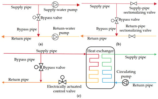
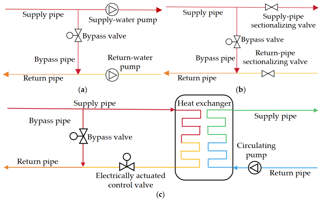
To exploit the thermal storage potential of the return network, this study adopts the bypass thermal storage method proposed in our previous study [23]. Bypass pipes connecting the supply and return pipes are installed at selected stations, converting these stations into bypass nodes. The bypass pipes divert part of the high-temperature supply water into the return network. This increases the average return-water temperature and enhances the DHN’s thermal storage and thermal-release capabilities. The structures of the bypass nodes are shown in Figure 1. Different line colors indicate the temperature levels of the heat-transfer medium in the corresponding pipes. In a long-distance DHN, the bypass nodes may be relay pumping stations, valve chambers, or the terminal energy station. In an urban primary DHN, bypass nodes are generally located at heating substations. An electrically actuated control valve is installed on each bypass pipe to regulate the bypass flow rate.
Figure 1.
Structures of different types of bypass nodes. (a) Booster pumping station; (b) valve chamber; (c) heat exchange node (energy station or heating substation).
Under the thermal storage condition, the supply-water temperature at the heat source is increased from its reference value to the thermal storage temperature. When the high-temperature heat-transfer medium reaches a bypass node, part of it enters the return network. The remainder continues through the supply pipe or enters the heat exchanger to meet the user heat demand. At bypass node i, heat-transfer media at different temperatures are assumed to mix instantaneously and completely. According to the energy balance, the return-water temperature after mixing is:
where i is the bypass node index; Gr,in is the low-temperature return-water flow rate before mixing, in t/h; Gb is the bypass flow rate, in t/h; Tr,in is the low-temperature return-water temperature before mixing, in °C; Ts,hs is the supply-water temperature under the thermal storage condition, in °C; Tr,out is the return-water temperature after mixing, in °C.
As the high-temperature heat-transfer medium completes its passage through the supply and return networks, the temperature and flow distributions in the DHN gradually stabilize, and the network enters the thermal storage saturation condition. At this point, the total thermal energy stored in the network using the bypass thermal storage method can also be calculated using Equation (2). By diverting part of the high-temperature supply water into the return network through the bypass branches, the method increases the average temperature of the return-water medium under the thermal storage saturation condition. The return network thus stores part of the thermal energy, increasing the total thermal energy stored in the DHN.
At the beginning of thermal release, the heat-source supply-water temperature is gradually reduced to its reference value within the prescribed ramp-rate limit, while the bypass control valves are closed to reduce the bypass flow rate to zero. The high-temperature heat-transfer medium produced during the preceding thermal storage process continues to flow through the supply and return networks, and the thermal energy stored in both networks is gradually released. During this process, the instantaneous thermal output of the heat source is reduced to:
where τ is time, in h; Qsc,hr is the thermal output of the heat source under the thermal-release condition, MW; Gsc,hr is the total circulating flow rate at the heat source under the thermal-release condition, in t/h; Tscs,ref is the reference supply-water temperature at the heat source, in °C; Tscr,hr is the return-water temperature at the heat source under the thermal-release condition, in °C.
In practical applications, the locations and flow rates of the thermal storage bypasses determine the extent of network thermal storage and the magnitude of the increase in return-water temperature. These factors are constrained by the network topology, pump delivery capacity, and other operating conditions. The bypass configuration and flow rates must therefore be optimized according to the operating conditions of the DHN and the economic objective.
3. Economic Performance of Combined Heat and Power Units
3.1. Components of Combined Heat and Power Unit Operating Profit
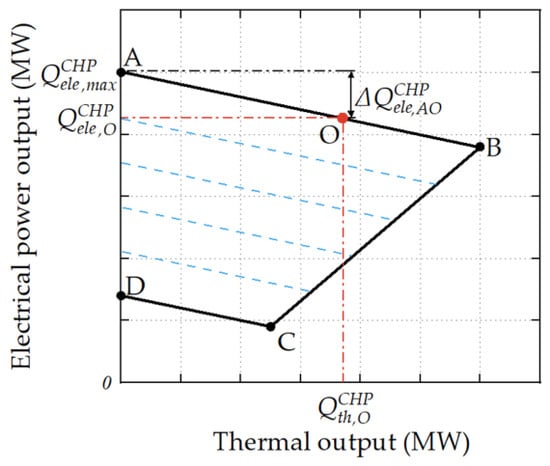
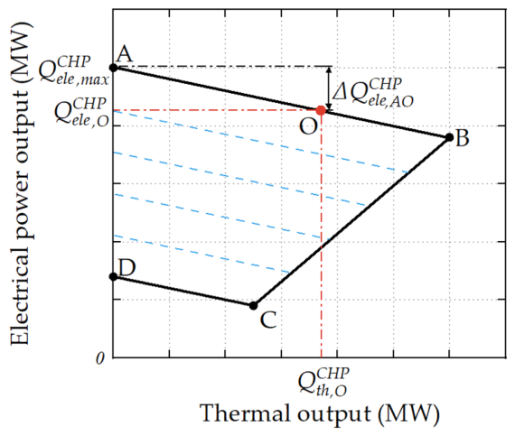
The thermal and electrical outputs of an extraction-condensing CHP unit are jointly constrained by the steam-turbine configuration, boiler load, heating demand, and other factors. Its operating region is shown in Figure 2. Points A and D denote the maximum and minimum electrical-power output points, respectively, under condensing-only operation. Point B denotes the maximum heat-output point, whereas point C denotes the minimum electrical-power output point. The black solid line delineates the operating region of the CHP unit, and the red dash-dotted lines indicate the coordinate projections of operating point O. The blue dashed lines approximately parallel to line AB within the operating region represent constant boiler input power.
Figure 2.
CHP operating region.
To describe the coupling between the thermal and electrical outputs of the unit, the overall electrical efficiency of the CHP unit is defined as:
where ηCHPele is the overall electrical efficiency of the CHP unit; QCHPele is the electrical power output of the unit, in MW; QCHPinput is the input power of the unit, in MW. Because thermal output occupies part of the power-generation capacity available under condensing-only operation, the constant-input-power lines and boundary AB both have negative slopes. The specific electrical power loss ζ can be expressed as:
where ΔQCHPele,AO is the reduction in total electrical power output, in MW; QCHPth,O is the thermal output at point O, in MW. Based on the specific electrical power loss, the thermal output is converted into an equivalent electrical output under condensing-only operation, and the equivalent electrical load ratio is then obtained to characterize the overall load level of the unit:
where QCHPele,equ is the equivalent electrical output under condensing-only operation, in MW; QCHPele,max is the maximum electrical output under condensing-only operation, in MW; θele,equ is the equivalent electrical load ratio.
As the electrical load ratio decreases, the standard coal consumption rate gradually increases [27]. The load-dependent coal consumption coefficient is therefore expressed as [28]:
where FCfuel is the coal consumption coefficient, and αfuel,1, αfuel,2, and αfuel,3 are coefficients obtained by fitting. Considering electricity-sales revenue, heat-sales revenue, and fuel costs, the operating profit of the CHP unit is expressed as:
where NBop is the operating profit of the CHP unit from electricity and heat sales after deducting fuel costs, in yuan; τst and τend are the starting and ending times of CHP unit operation, respectively, in h; Cele is the electricity price, in yuan/MWh; Cth is the heat-selling price, in yuan/MWh; Cfuel is the fuel cost per unit of lower heating value, in yuan/MWh.
3.2. Economic Conversion of Power Flexibility Under Different Market Mechanisms
When a DHN releases stored thermal energy during a peak- or valley-price period, the instantaneous thermal output of the CHP unit can be reduced while user heat demand remains satisfied. The reduction in the instantaneous thermal output of the heat source resulting from thermal release by the network can be expressed as:
where ΔQth,hr is the reduction in the thermal output of the heat source, in MW; QCHPth,ref and Q CHPth,hr are the reference and actual thermal outputs, respectively, in MW.
In the peak-shaving ancillary services market, the unit participates in power-grid peak shaving mainly by reducing its electrical load ratio. The actual electrical load ratio of the unit is defined as:
where θele is the actual electrical load ratio, and QCHPele is the actual electrical power output, in MW.
After thermal release from the district heating network reduces the thermal output of the unit, its operating point can move along line BC in Figure 2 toward lower thermal and electrical outputs. The resulting change in electrical power output can be expressed as:
where ΔQCHP,BCele,hr is the change in the electrical power output of the unit under the peak-shaving ancillary services mechanism, in MW; αBC,1 is the slope of the back-pressure operating line BC.
When the actual electrical load ratio is lower than the reference load ratio for peak-shaving compensation, the portion of the electrical output below the reference value can be regarded as eligible peak-shaving capacity. The peak-shaving ancillary service revenue can be calculated as:
where NBps is the peak-shaving ancillary service revenue, in yuan; Cps is the peak-shaving compensation rate, in yuan/MWh; θele,ps is the reference load ratio for peak-shaving compensation; [x]+ = max(x,0).
In the electricity spot market, the operating direction of the unit depends on the clearing price. In this study, the operating conditions of the unit are classified using the break-even electricity price and the critical heat-compensation electricity price. The break-even electricity price is defined as the electricity price at which the sum of heat-sales revenue and electricity-sales revenue from the CHP unit is exactly equal to its fuel cost. When the clearing price is lower than the break-even electricity price, the unit’s operating revenue is insufficient to cover its fuel cost, and its most economical operating point tends toward point C in Figure 2. This condition is defined as the valley-price condition.
The critical heat-compensation electricity price is the price at which the additional electricity-sales revenue from increasing electrical output along the constant-input-power line AB equals the corresponding reduction in heat-sales revenue. Above this price, increasing electrical output is more profitable than increasing thermal output, and the optimal operating point tends toward point A. This condition is defined as the peak-price condition.
Using the reference condition as the benchmark, the changes in the electrical power output of the unit resulting from thermal release by the network can be expressed uniformly as:
where ΔQCHP,PPCele,hr and ΔQCHP,VPCele,hr are the changes in the electrical power output of the unit under the peak-price and valley-price conditions, respectively, in MW.
Under either of the above market mechanisms, the total operating profit of the CHP unit can be expressed as:
where NBtotal is the total operating profit of the CHP unit, comprising NBop and the peak-shaving ancillary service revenue, NBps, in yuan.
Under the electricity spot market, NBps = 0 in Equation (16). The electrical power output, thermal output, and corresponding market prices under the reference and thermal-release conditions are substituted into Equation (10) to calculate the total profit of the unit under each condition. For either market mechanism, the operating-profit increment is the difference in NBtotal between the thermal-release and reference conditions over the same period. Under the peak-shaving ancillary services mechanism, this increment includes the change in ancillary service revenue.
4. Construction of Typical Operating Scenarios
4.1. Typical Electricity-Price Scenarios and Representative Weights
In the electricity spot market, clearing-price profiles usually vary considerably from day to day. Therefore, Monte Carlo simulation and clustering are used to obtain typical electricity-price scenarios and calculate their representative weights over the entire heating season.
First, historical real-time clearing prices during the heating season are divided into daily electricity-price profiles. The real-time electricity price is updated every 15 min, and each daily profile contains 96 time intervals. Monte Carlo sampling is then performed according to the empirical price distribution in each interval and the correlations among different intervals, generating a set of scenarios that reflects electricity-price fluctuations during the heating season. Specifically, the empirical marginal distribution is estimated separately for each time interval, and a Gaussian copula is used to represent the dependence among the 96 intervals. A rank-based probability transform is applied to obtain normal scores and estimate the correlation matrix. Correlated normal samples are then transformed back through the empirical marginal distributions to generate the simulated price profiles.
Second, candidate numbers of clusters, corresponding to the numbers of typical electricity-price scenarios, are selected sequentially within a predefined range, and k-means clustering is performed multiple times for each candidate number using different random initializations. In each run, each electricity-price profile is assigned to the nearest cluster centroid according to the Euclidean distance, and each centroid is updated as the mean profile of the assigned samples. These assignment and centroid-update steps are repeated until the clustering objective converges or the cluster labels remain unchanged.
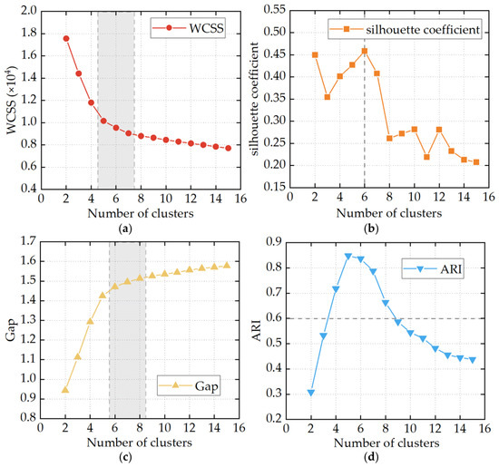
For each fixed candidate number k, within-cluster sum of squares (WCSS) is minimized during the iterative k-means procedure. After clustering is completed for each candidate k, the number of typical electricity-price scenarios is selected by comparing four indicators: WCSS, the silhouette coefficient, the Gap statistic, and the adjusted Rand index (ARI). The comparison considers within-cluster compactness, between-cluster separation, and clustering stability.
Finally, the complete Monte Carlo scenario set is clustered using k-means with the selected number of clusters. The centroid of each cluster is taken as a typical electricity-price profile, and the proportion of scenarios in that cluster relative to the total number of scenarios is taken as its representative weight:
where pk is the representative weight of the k-th typical electricity-price profile; Nk is the number of electricity-price scenarios in the k-th cluster; Nmt,total is the total number of scenarios generated by Monte Carlo simulation.
4.2. Typical Heat-Load Scenarios and Representative Weights
The daily average heat load of a heating system varies considerably over the heating season. Therefore, typical heat-load scenarios are constructed in this study. Although actual district-heating demand varies within a day [29], building thermal mass and end-use control can buffer part of these short-term fluctuations [30]. For the network-level analysis, the heat load for each representative day is therefore represented by the arithmetic mean of its hourly values. This value characterizes the average hourly demand for that day. Variations among different days are represented by different typical scenarios.
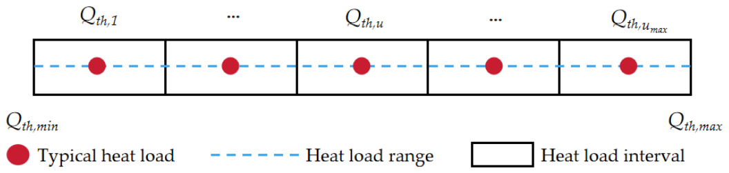
Based on the minimum and maximum values of the daily average heat-load samples during the heating season, the heat-load range is divided into several equal intervals. The midpoint of each interval is taken as the representative value of the corresponding typical heat-load scenario. The number of typical scenarios is determined by comprehensively considering the distribution of the heat-load samples, the accuracy of scenario representation, and the computational scale of the model. Specifically, candidate partitions with NH,min ≤ NH ≤ NH,max are evaluated using the normalized root-mean-square error:
where d indexes heating days; dtotal is the total number of days in the heating season; Qth,d is the daily mean heat load, in MW; is its assigned interval midpoint, in MW; is the mean of the daily heat loads over the heating season, in MW. A geometric trade-off score J(NH) is calculated as:
The candidate interval number NH that maximizes J(NH) is selected within the examined range. NRMSE quantifies the daily heat-load reconstruction error, while the interval weights preserve the occurrence frequencies of the corresponding heat-load ranges in the heating-season representation. Each nonempty interval defines a representative scenario.
The division of the typical heat loads and their representative ranges is shown in Figure 3.
Figure 3.
Division of typical heat loads and their representative ranges.
Each heating day is assigned to the corresponding typical scenario according to the interval containing its daily average heat load. The number of actual heating days in each interval is then counted, and the representative weight of each typical heat-load scenario is calculated as:
where pu is the representative weight of the u-th typical heat-load scenario, and du is the number of heating days included in the u-th typical heat-load scenario.
5. Bilevel Optimization Model for the Operating Profit of Combined Heat and Power Units
5.1. Model Structure
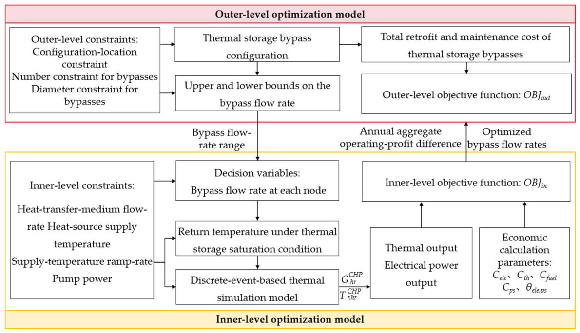
To configure thermal storage bypass devices and improve CHP economic performance, this study develops a bilevel optimization model. The model optimizes the bypass configuration and flow rates using CHP operating performance as the economic objective. The model procedure is shown in Figure 4.
Figure 4.
Flowchart of the bilevel optimization model.
The outer-level model generates feasible bypass-device configuration schemes. Each configuration specifies the bypass locations, number, and pipe diameters. The corresponding bypass flow-rate bounds are determined from the selected diameters and the allowable flow velocity and specific frictional resistance, and are passed to the inner-level model. For each configuration, bypass flow rates are optimized for each typical heat-load scenario in the peak-shaving ancillary services market. In the electricity spot market, flow rates are optimized for each heat-load–electricity-price scenario combination. The bypass configuration remains unchanged across scenarios. For each configuration and set of bypass flow rates, the dynamic thermal simulation model calculates changes in the supply- and return-water temperatures and flow rates of the DHN. The thermal output of the CHP unit is calculated from the heat-source supply–return temperature difference and circulating flow rate. The electrical output and total operating profit are then determined using the CHP operating region and the market-specific formulations in Section 3. Under the peak-shaving ancillary services mechanism, the total unit operating profit includes peak-shaving compensation. The operating-profit increment is calculated as the total operating profit under the thermal-release condition minus that under the reference condition without DHN thermal storage over the same period. These increments are aggregated using the scenario weights and heating-season duration, with the number of daily peak-shaving events also included for the ancillary services mechanism, to obtain the annual aggregate operating-profit increment.
The inner-level model returns the maximum annual aggregate operating-profit increment to the outer-level model. The outer-level model calculates the life-cycle net present value (NPV) by considering the bypass-device configuration and maintenance costs, and determines the final configuration scheme by comparing different candidate schemes. The inner-level model is solved using GlobalSearch in combination with fmincon, whereas the outer-level model is solved using a discrete search method. The optimization and dynamic thermal simulations were implemented in MATLAB R2026b. The outer-level search terminates after all feasible combinations within the specified candidate-node and pipe-diameter sets have been evaluated, subject to the bypass-number limits. The configuration with the highest net present value is selected. The input data, decision variables, objectives, constraints, solution methods, termination criteria, and outputs are summarized in Table 2.
Table 2.
Summary of the bilevel optimization model.
5.2. Outer-Level Optimization Model
The decision variables of the outer-level model include the installation locations, number, and pipe diameters of the thermal storage bypass devices. The objective is to maximize the life-cycle NPV. For a given thermal storage bypass configuration, the retrofit cost is expressed as:
where Cb,reform is the retrofit cost of the thermal storage bypasses, in yuan; κi is a binary indicator of whether a bypass is installed at candidate node i, with κi = 1 when a bypass device is installed at the node, and κi = 0 otherwise; Cib,pipe is the bypass-pipe cost at candidate node i, in yuan; Cib,val is the bypass-valve cost at candidate node i, in yuan; Cib,others is the cost of other materials and associated construction at candidate node i, in yuan.
The total life-cycle cost of the bypasses, Cb,total (ω), consists of the total present value of maintenance costs and the retrofit cost:
where Cb,mt is the present value of the life-cycle maintenance costs, discounted to the start of the analysis period, in yuan.
Based on the annual aggregate operating-profit increment obtained from the inner-level model, the net present value of configuration scheme ω is calculated as:
where NPV is the life-cycle net present value (NPV) of the bypass retrofit, in yuan; ΔNBay is the annual aggregate operating-profit increment relative to the reference condition without DHN thermal storage, including the ancillary service revenue increment under the peak-shaving mechanism, in yuan, as determined by the inner-level model; PVAF is the present value annuity factor; r is the annual interest rate; and y is the number of years in the analysis period, which is taken as the service life of the thermal storage bypass devices in this study. The product PVAF ·ΔNBay represents the life-cycle present value of the operating-profit increments; subtracting the retrofit cost and the present value of maintenance costs gives the NPV.
The outer-level optimization model selects the thermal storage bypass configuration with the maximum NPV as the final optimization result, thereby maximizing the life-cycle net economic benefit of the bypass retrofit. Its objective function OBJout is:
The constraints of the outer-level model include the configuration-location constraint, the number constraint for thermal storage bypasses, and the bypass-pipe diameter constraint. These constraints limit the candidate nodes eligible for retrofit, the permissible range of the number of bypass installations, and the available bypass-pipe diameter specifications, respectively. They are expressed uniformly as:
where Numb,min and Numb,max are the minimum and maximum permissible numbers of bypass installations, respectively; Numb is the total number of thermal storage bypass installations; Dbi is the bypass-pipe diameter, m; Dstd is the set of standard pipe diameters, m.
5.3. Inner-Level Optimization Model
The decision variable of the inner-level model is the bypass flow rate. The bypass flow rate changes the DHN temperature distribution under the thermal storage saturation condition. It also affects the thermal-release process and, consequently, the thermal and electrical outputs and operating profit of the CHP unit. Therefore, the objective of the inner-level model is to maximize the annual aggregate operating-profit increment.
Using the reference condition without DHN thermal storage as the benchmark, the single-event operating-profit increment in the peak-shaving ancillary services market is the difference between total operating profit under the thermal-release condition and that under the reference condition. In the electricity spot market, the peak- and valley-price increments are calculated in the same way for their respective operating conditions. The annual aggregate operating-profit increment under the two market mechanisms is calculated as:
where Mps is the number of peak-shaving events per day; ΔNBtotal(u) is the single-event operating-profit increment under the peak-shaving ancillary services market, in yuan; ΔNBPPCop(k,u) is the operating-profit increment during the peak-price period under the k-th typical electricity-price scenario and the u-th heat-load scenario, in yuan; ΔNBVPCop(k,u) is the operating-profit increment during the valley-price period under the k-th typical electricity-price scenario and the u-th typical heat-load scenario, in yuan.
The objective of the inner-level optimization model is to maximize the annual aggregate operating-profit increment. Its objective function OBJin is:
The inner-level model ensures the safe operation of the district heating network through constraints on the heat-transfer-medium flow rate, heat-source supply-water temperature, and pump power. The heat-transfer-medium flow rate must remain within the permissible range for the corresponding pipe diameter. The upper and lower flow-rate limits are determined according to the pipe diameter, allowable specific frictional resistance, and maximum flow velocity. The heat-source supply-water temperature must not exceed the permissible values of the network and equipment. In addition, the pump power under the thermal storage condition must not exceed that under the reference condition. To prevent excessively rapid supply-temperature adjustment from affecting system stability, the ramp rate of the heat-source supply-water temperature during thermal release is also constrained. These constraints are expressed uniformly as:
where Tscs,max is the maximum heat-source supply-water temperature, in °C; Gn,min and Gn,max are the minimum and maximum flow rates in pipe section n, respectively, in t/h; Qp,hs and Qp,ref are the pump powers under the thermal storage saturation condition and the reference condition, respectively, in MW; RaT,s is the maximum permissible ramp rate of the heat-source supply-water temperature, in °C/h. In this study, RaT,s = 10 °C/h [31].
During the optimization process, a discrete-event-based dynamic thermal simulation method is used to calculate the time-varying temperature and flow-rate processes in the district heating network [32]. Hydraulic changes are represented by successive steady states because pressure disturbances propagate much faster than temperature disturbances [33]. Water is treated as incompressible, with constant density and specific heat capacity. Flow rates are updated as operating conditions change, satisfying nodal mass continuity and network pressure balance.
Hydraulic resistance parameters are estimated from design data. For an active bypass branch at node i, pipe friction and the local losses associated with the control valve and fittings are represented by an equivalent hydraulic resistance:
where Δpb(i) is the bypass pressure loss, Pa; λb(i) is the Darcy friction factor; Lb(i) is the bypass length, m; Db,in(i) is the internal diameter corresponding to the selected bypass-pipe size, m. The coefficients ξb,val(i) and ξb,l(i) represent the local losses of the control valve and fitting l, respectively. vb(i) is the flow velocity, m/s, and Sb(i) is the equivalent resistance coefficient, Pa/(t/h)2.
These branch pressure losses enter the network pressure-balance equations, linking bypass-flow redistribution to the required pump pressure rise. The electrical input power of the pump is calculated as:
where Δpp is the pump pressure rise, Pa; Gp is the mass flow rate through the pump group, in t/h; and ηp is the adopted overall efficiency. The resulting Qp is expressed in MW.
The thermal model assumes one-dimensional plug flow, with uniform velocity and temperature across each pipe cross-section and negligible axial mixing and conduction [10,34]. Incoming streams mix instantaneously and completely at junctions, and thermal losses are calculated using equivalent thermal resistances. This method accurately describes the propagation delay and attenuation of the heat-transfer-medium temperature and has relatively high computational efficiency, making it suitable for repeated evaluations during the inner-level optimization process.
6. Engineering Case Studies
6.1. Project Overview
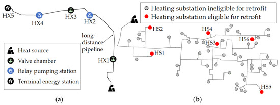
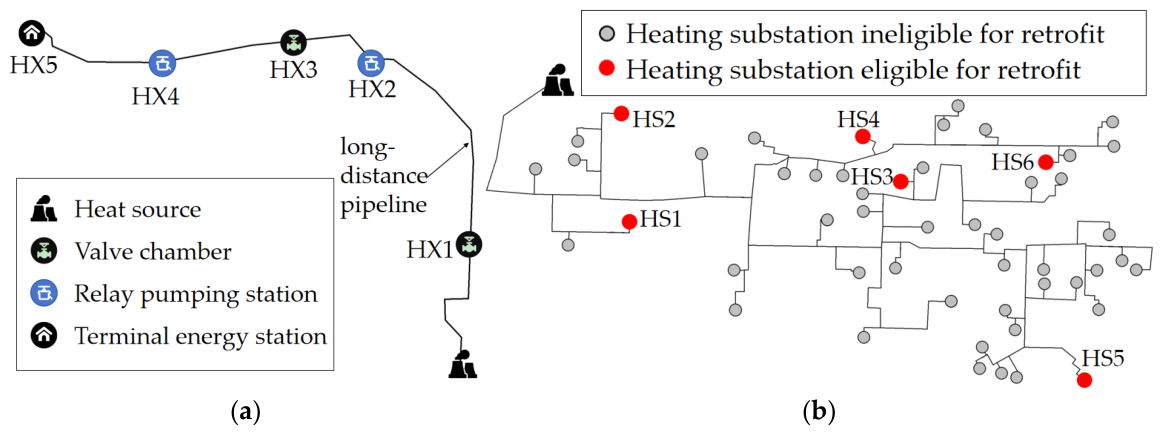
An actual long-distance district heating network in Chengde (Hebei Province, China) and an actual primary district heating network in Jinchang (Gansu Province, China) are selected to evaluate the economic performance of the bypass thermal storage method. Their topologies are shown in Figure 5. The long-distance network has a total length of 24.9 km and contains five candidate nodes, HX1–HX5, at which bypass devices can be installed. The peak-shaving ancillary services market provides incentives for the CHP unit to participate in peak shaving. The primary district heating network contains 51 heating substations and has a total heated floor area of approximately 7.38 million m2. Two heating substations in each of the near-source, intermediate, and distant regions are eligible for thermal storage bypass installation. These six substations are numbered HS1–HS6. The primary network operates under the electricity spot market mechanism.
Figure 5.
Topologies of the district heating networks. (a) Topologies of the long-distance DHN; (b) Topologies of the primary DHN.
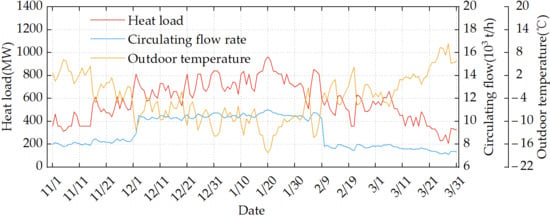
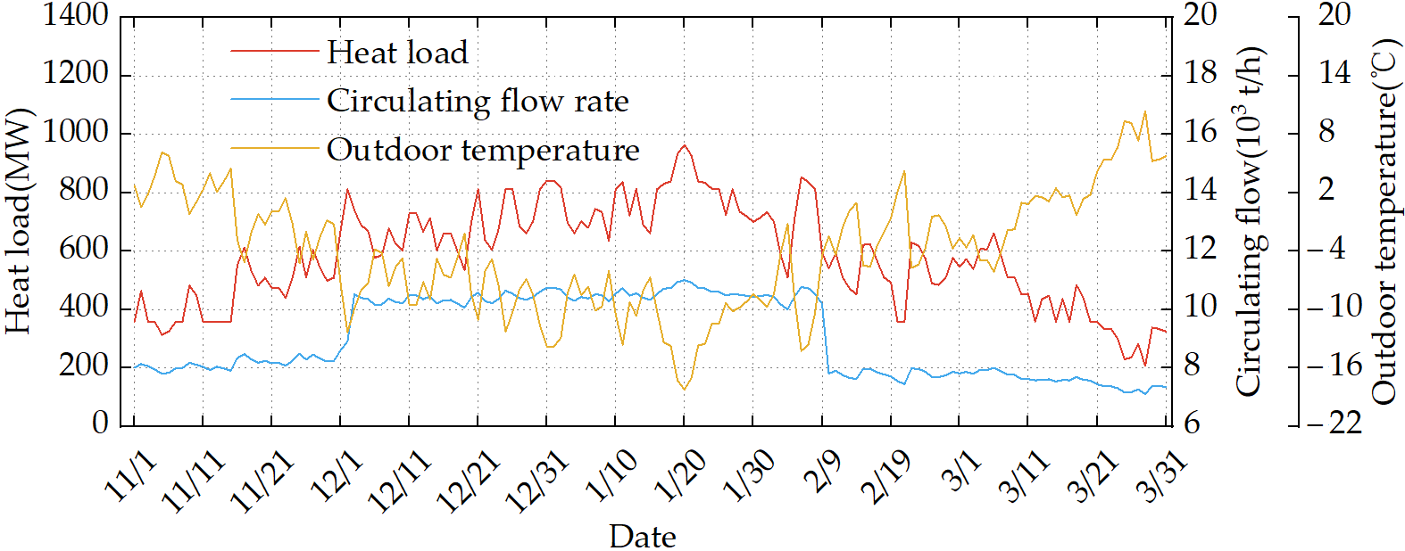
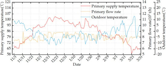
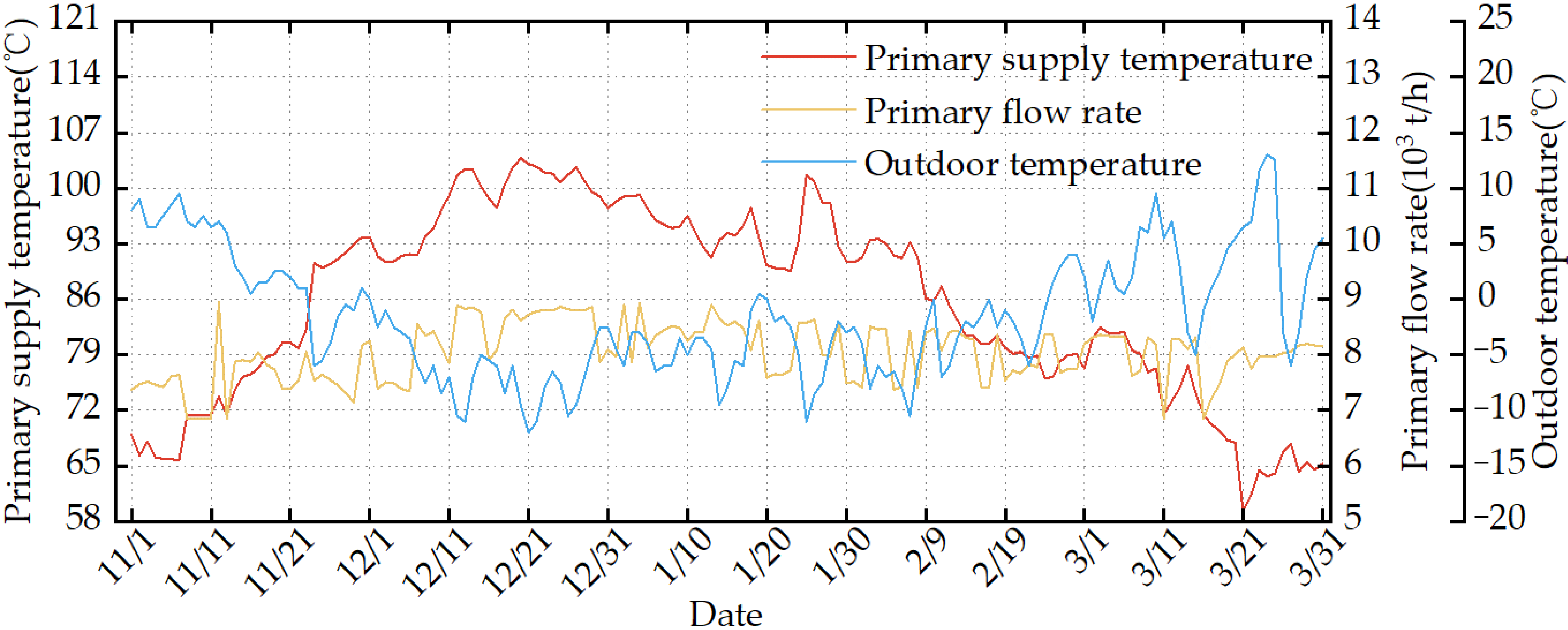
The heating season for both networks lasts 151 days. Hebei has a temperate monsoon climate with cold, dry winters. Gansu has a temperate continental arid climate characterized by low precipitation, abundant sunshine, and dry, windy conditions. During the corresponding heating seasons, the seasonal averages of daily mean outdoor temperature were −4.11 °C in Hebei and −1.51 °C in Gansu. The temperature ranges were −18.23 to 10.38 °C and −12.07 to 13.28 °C, respectively. Figure 6 and Figure 7 show the variations in key heating-system parameters and daily mean outdoor temperature for the long-distance DHN and urban primary DHN, respectively. The typical heat-load scenarios for the long-distance and primary district heating networks are presented in Table 3 and Table 4, respectively.
Figure 6.
Key heating parameters of the long-distance DHN and outdoor temperature.
Figure 7.
Key heating parameters of the primary DHN and outdoor temperature.
Table 3.
Typical heat-load scenarios for the long-distance district heating network.
Table 4.
Typical heat-load scenarios for the primary district heating network.
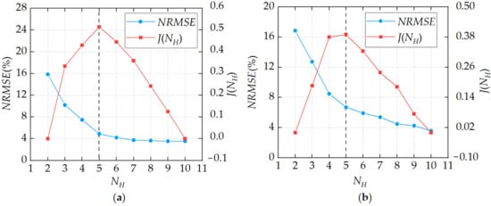
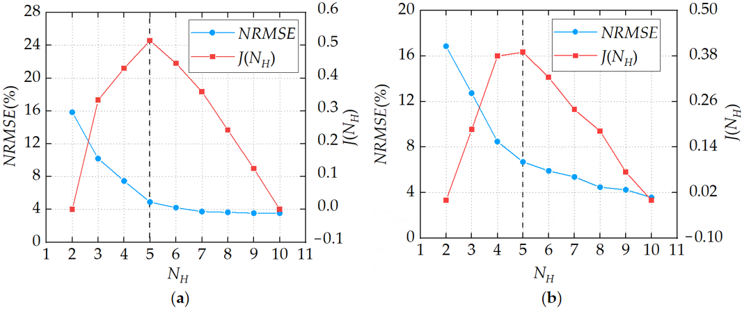
Candidate interval numbers from NH,min = 2 to NH,max = 10 were evaluated for both DHNs. Figure 8 compares the NRMSE and geometric trade-off score J(NH) for the two DHNs. For the long-distance DHN, the NRMSE decreases from approximately 15.8% at NH = 2 to 4.9% at NH = 5, while J(NH) reaches its maximum of approximately 0.51 at NH = 5. Further increasing the number of intervals to NH = 10 reduces the NRMSE to approximately 3.5%, but the additional reduction is relatively limited, and the trade-off score decreases.
Figure 8.
Normalized root-mean-square errors and geometric trade-off scores. (a) Long-distance DHN; (b) urban primary DHN.
For the urban primary DHN, the NRMSE decreases from approximately 16.9% at NH = 2 to 6.7% at NH = 5, and J(NH) reaches its maximum of approximately 0.39 at NH = 5. Although NH = 10 produces a lower NRMSE of approximately 3.6%, the improvement is accompanied by a substantially larger number of representative scenarios. Therefore, considering both daily reconstruction accuracy and the increase in scenario number, NH = 5 was selected for both DHNs. The corresponding five nonempty intervals were used to construct the representative heat-load scenarios listed in Table 3 and Table 4.
Under the thermal storage condition, the heat-source supply-water temperature is set 5 °C above its reference value. During severe cold periods, the maximum available temperature margin between the reference heat-source supply-water temperature and the allowable maximum supply-water temperature is approximately 6 °C for the two networks. Therefore, a 5 °C temperature rise was selected as a feasible thermal-storage setting that satisfies the temperature limit while retaining an operating margin under the investigated conditions. The heat-selling price is 118.80 yuan/MWh, and the fuel cost is 109.42 yuan/MWh.
Under the peak-shaving ancillary services mechanism applied to the long-distance district heating network, the fixed electricity price is 360.00 yuan/MWh, and the reference load ratio for peak-shaving compensation is 0.5. The peak-shaving ancillary services market is activated for 7 h, Mps = 1. The peak-shaving compensation rate is divided into four tiers according to the load ratio, as detailed in Table 5.
Table 5.
Peak-shaving compensation rates.
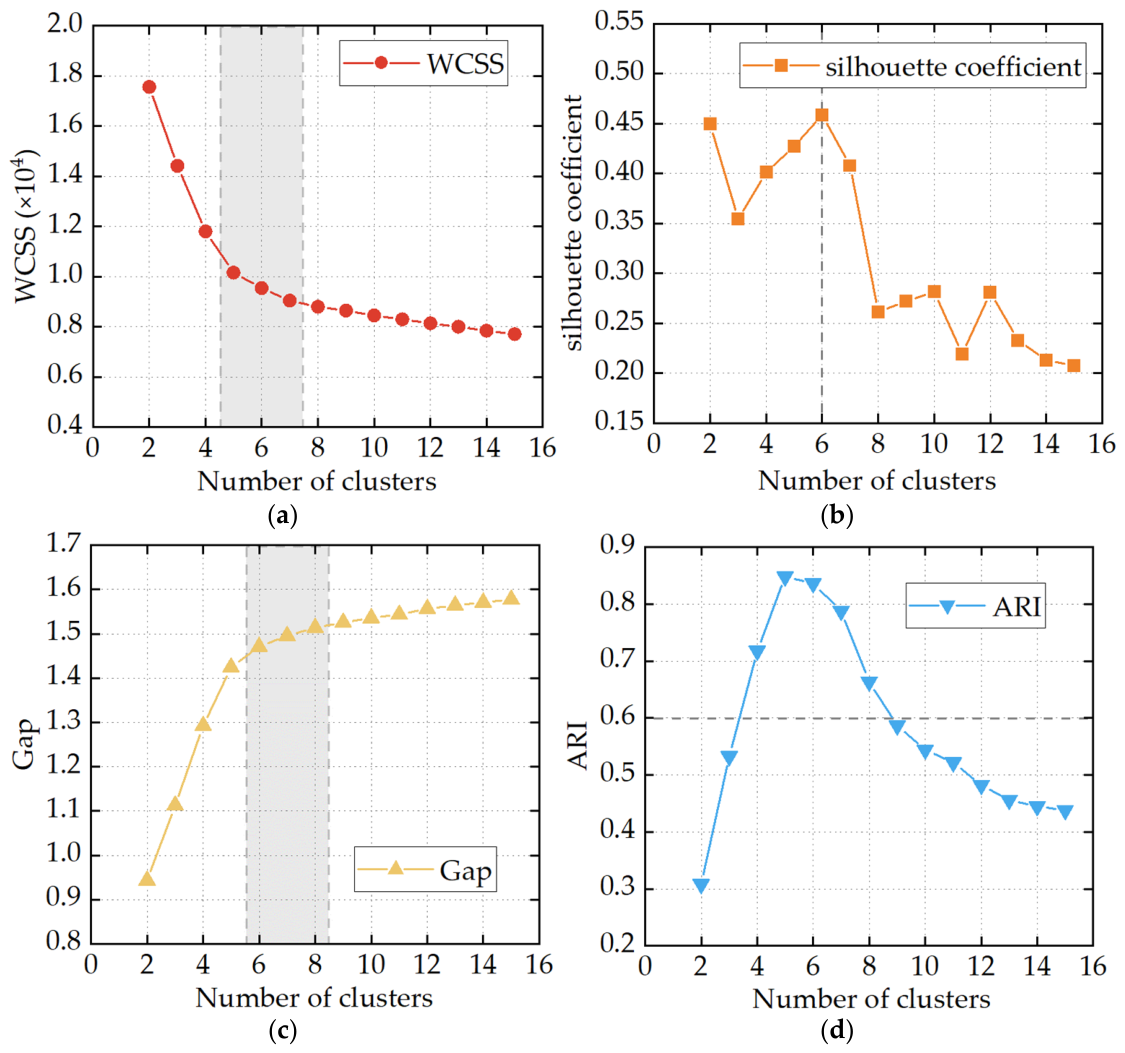
For this case, the historical real-time clearing-price data cover the heating season from 1 November 2024 to 31 March 2025. The dataset contains 151 daily profiles, each with 96 15 min observations, giving 14,496 historical price observations. Following the procedure in Section 4.1, 2000 Monte Carlo scenarios were generated, and candidate cluster numbers from 2 to 15 were evaluated. As shown in Figure 9, the WCSS curve exhibits an elbow around k = 5–7, while the silhouette coefficient reaches its maximum at k = 6. The gray dashed box in Figure 9a highlights the relatively favorable range of k values around the WCSS elbow, whereas the gray dashed line in Figure 9b marks the k value corresponding to the highest silhouette coefficient. The Gap statistic increases with k, but its improvement becomes limited beyond approximately k = 6–8. The gray dashed box in Figure 9c highlights the relatively favorable range identified from the Gap statistic. The ARI remains above 0.8 for k = 5–6, indicating stable clustering in this range. The gray dashed line in Figure 9d indicates the minimum acceptable ARI level. Considering the four indicators jointly, k = 6 was selected as a balance between clustering quality, stability, and scenario-reduction efficiency.
Figure 9.
Cluster-number evaluation. (a) WCSS; (b) silhouette coefficient; (c) Gap; (d) ARI.
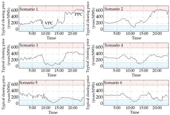
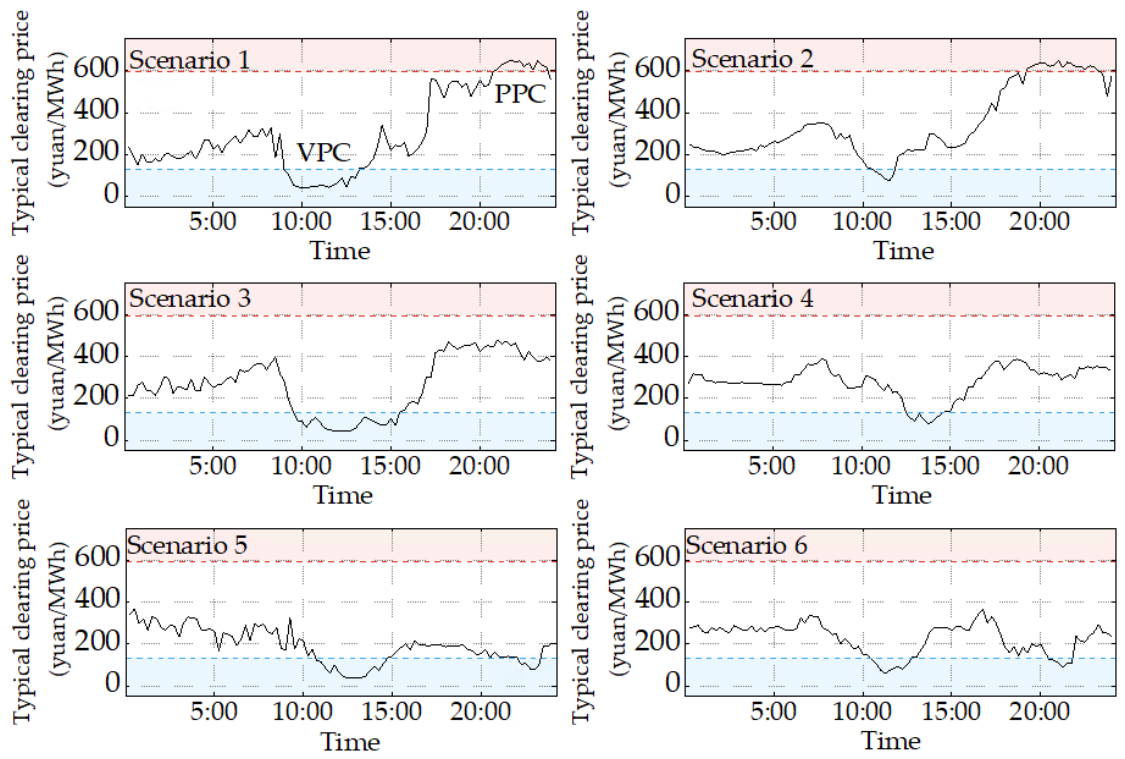
Under the electricity spot market mechanism applied to the primary district heating network, the break-even electricity price is 131 yuan/MWh, and the critical heat-compensation electricity price is 593 yuan/MWh. The resulting six typical market-clearing electricity-price scenarios are shown in Figure 10. The red-shaded area represents the peak-electricity-price region, the blue-shaded area represents the valley-electricity-price region, and the black curve represents the market-clearing electricity-price curve. The total costs of bypasses with different specifications are listed in Table 6.
Figure 10.
Typical clearing-price scenarios.
Table 6.
Total costs of thermal storage bypass configurations.
The robustness of the inner-level optimization was also examined using 50 feasible starting points, including the two bound points, their midpoint, and randomly sampled points within the variable bounds. Convergence was achieved in 47 runs (94%), and the best feasible converged result was used for the reported optimization results.
These cases were selected to examine different network structures and electricity-market mechanisms. In the long-distance DHN, water is transported mainly along the transmission main to the terminal energy station, and bypass locations affect the return-water transport paths and travel times. In the urban primary DHN, return flows from multiple branches and distributed heating substations mix before reaching the heat source. These structural differences and the respective market mechanisms provide distinct engineering settings for evaluating bypass configuration and flow-rate optimization.
6.2. Thermal Storage Bypass Configurations
Table 7 presents the optimal bypass configuration for the long-distance district heating network under the peak-shaving ancillary services market. The bypasses are installed at relay pumping station HX4 and terminal energy station HX5, both of which are relatively far from the heat source. The bypass flow is concentrated mainly at terminal node HX5, while HX4 serves an auxiliary function. These results indicate that, under the peak-shaving duration and hydraulic conditions considered in this case, the bypass configuration tends to utilize the intermediate and distant return-water transport paths.
Table 7.
Thermal storage bypass configuration results for the long-distance district heating network.
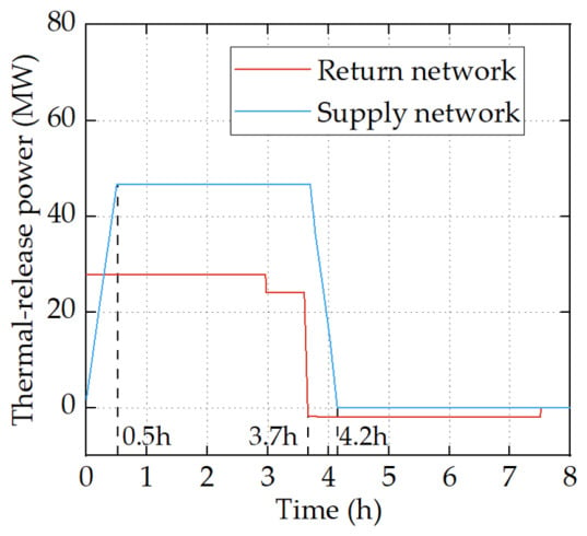
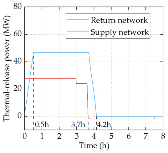
For the HC3 scenario of the long-distance district heating network, the thermal-release power of the network is shown in Figure 11. The dashed lines indicate the projections of the key transition points onto the x-axis. At the beginning of thermal release, the high-temperature return water gradually returns to the heat source, resulting in relatively high thermal-release power from the return network. As the heat-source supply-water temperature gradually decreases, the thermal-release power of the supply network increases.
Figure 11.
Thermal-release process of the long-distance district heating network.
Subsequently, the thermal-release power of the return network gradually decreases, and the return network enters a recharging state. Because of transport delay, some heat-exchange nodes still receive high-temperature supply water during thermal release, producing return water below the reference temperature. This low-temperature return water first causes additional thermal release. Recharging begins only when subsequent return water at the reference temperature replaces it and increases the stored heat, causing the thermal-release power to become negative. The supply network continues to release heat at a certain power until the state of the supply-water heat-transfer medium is restored. Thus, the supply and return networks release heat simultaneously during the initial stage of peak shaving, reducing the instantaneous thermal output of the heat source.
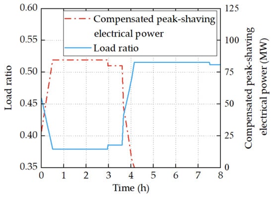
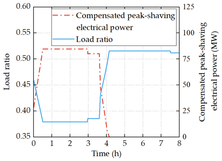
Figure 12 further shows the variations in the load ratio and compensated peak-shaving electrical power of the unit in the long-distance district heating network. After thermal release begins, the thermal output of the heat source decreases, and the unit load ratio falls into the compensation range of the peak-shaving ancillary services market, thereby increasing the compensated peak-shaving electrical power. As the thermal-release power of the network gradually decreases, the unit load ratio progressively recovers, accompanied by a corresponding decrease in compensated peak-shaving electrical power. This process shows that thermal release from the network can effectively reduce the electrical power output and load ratio of the unit during peak shaving.
Figure 12.
Load ratio and compensated peak-shaving electrical power of the CHP unit during thermal release.
For the urban primary district heating network operating under the electricity spot market mechanism, the optimal configuration results are presented in Table 8. The bypass configuration of the primary network must account for the transport capacity and hydraulic conditions of different branches under different typical thermal and electrical scenarios. It cannot be determined solely according to the distance between each node and the heat source. The heating substations equipped with bypasses are distributed among the near-source, intermediate-to-distant, and distant branches. The bypass flow is concentrated mainly at heating substations HS4 and HS6, while heating substation HS1 serves an auxiliary function.
Table 8.
Thermal storage bypass configuration results for the primary district heating network.
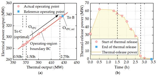
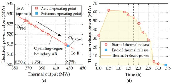
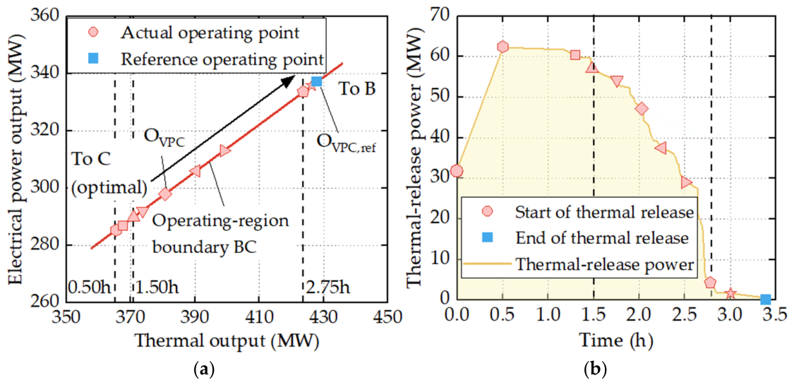
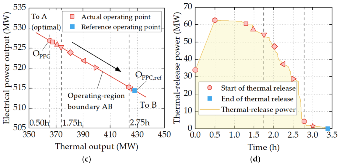
Taking the HY4 typical heat-load scenario as an example, Figure 13 shows the unit operating points and the thermal-release power under the valley-price condition (VPC) in typical electricity-price scenario 1 and under a peak-price condition (PPC). The black dashed lines highlight the key representative points, and the corresponding times are indicated in panels (a) and (c). During thermal release, the unit operating point moves toward point C under the valley-price condition and toward point A under the peak-price condition. These movements correspond to the regulation directions under low and high electricity prices, respectively. Because of the ramp-rate constraint on the heat-source supply-water temperature, the thermal-release power gradually increases during the initial stage. As thermal release from the network proceeds, the thermal-release power gradually decreases, and the unit operating point moves back toward the reference condition. After thermal release ends, the unit returns to the reference operating point.
Figure 13.
Changes in operating points and thermal-release power during valley- and peak-price periods. (a) Operating points under the VPC; (b) thermal-release power under the VPC; (c) operating points under the PPC; (d) thermal-release power under the PPC.
6.3. Field Validation of the Dynamic Thermal Simulation Model
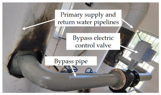
A field test was conducted in the urban primary DHN in Gansu Province following implementation of the optimized bypass configuration described in Section 6.2. Figure 14 shows the bypass installation at heating substation HS1 as an example. The bypass pipe connects the primary supply and return pipes, and an electrically actuated control valve regulates the bypass flow rate.
Figure 14.
Thermal storage bypass installation at heating substation HS1.
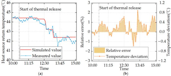
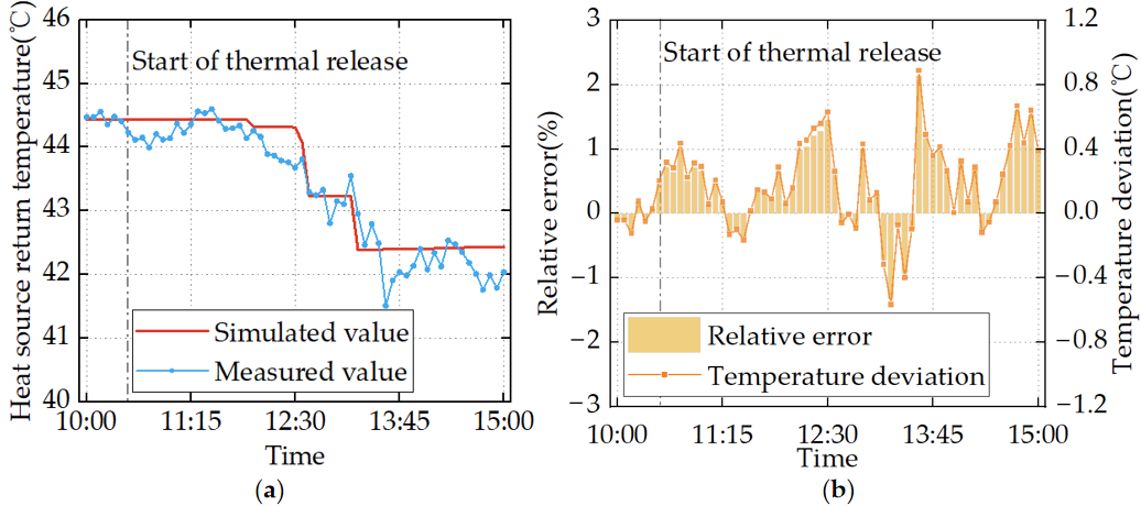
The test used the optimized bypass flow rates for heat-load scenario HY4 under a valley-price condition lasting 2.25 h. The bypass valves were closed at 10:30 to initiate thermal release. The primary return-water temperature was measured at the heat source at 5 min intervals, and the simulated temperature was evaluated at the same location and sampling times. During the preceding stable period, from 10:00 to 10:30, the simulated and measured primary supply- and return-water temperatures differed by no more than 0.2 °C. This agreement indicates that the simulated and actual initial operating states were closely matched.
Figure 15 compares the simulated and measured primary return-water temperatures and presents the corresponding errors. The gray dash-dotted line marks the start of thermal release. The model reproduced the overall temperature decline and the main transitions during thermal release. The measured curve shows minor fluctuations, whereas the simulated curve is smoother and more stepwise, partly reflecting simplified valve adjustments and the 0.05 °C temperature-change threshold used in the simulation. Measurement uncertainty may also contribute to these differences. The mean absolute error (MAE) was 0.25 °C, and the maximum absolute error was 0.89 °C. The mean absolute percentage error (MAPE) and maximum absolute percentage error were 0.58% and 2.14%, respectively. These results support the model’s ability to describe the dynamic response of the primary return-water temperature during bypass-assisted thermal release in the urban primary DHN under the tested condition.
Figure 15.
Validation of the primary return-water temperature at the heat source. (a) Simulated and measured temperatures; (b) temperature errors.
6.4. Economic Analysis
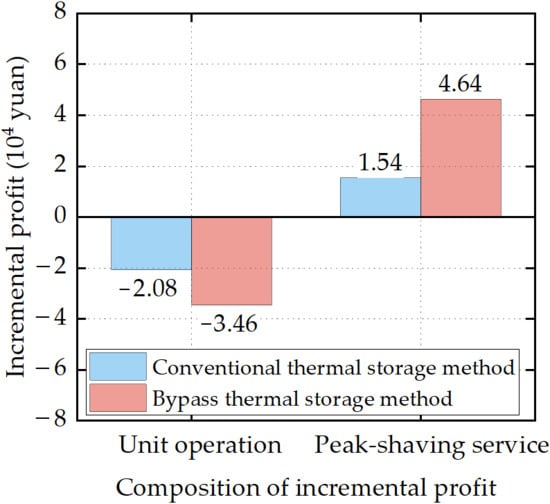
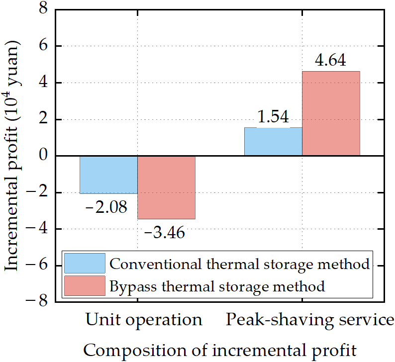
Figure 16 compares the incremental profit per peak-shaving event for the two thermal storage methods under typical heat-load scenario HC3 of the long-distance district heating network. With the conventional district heating network thermal storage method, the unit operating profit decreases by 20,800 yuan, while the peak-shaving ancillary-service revenue increases by 15,400 yuan. The compensation revenue is insufficient to offset the loss in unit operating profit, resulting in a decrease of 5400 yuan in total operating profit per event. With the bypass thermal storage method, the unit operating profit decreases by 34,600 yuan, but the peak-shaving ancillary-service revenue increases by 46,400 yuan, resulting in an increase of 11,800 yuan in total operating profit per event. Under the conventional district heating network thermal storage method, the peak-shaving compensation revenue cannot offset the reduction in unit operating profit, whereas the NPV reaches 10.8621 million yuan with the bypass thermal storage method. Thus, although the bypass thermal storage method causes greater losses in heat-sales and electricity-sales revenue, it ultimately yields a positive NPV through peak-shaving compensation.
Figure 16.
Changes in peak-shaving ancillary-service revenue and unit operating profit under different thermal storage methods.
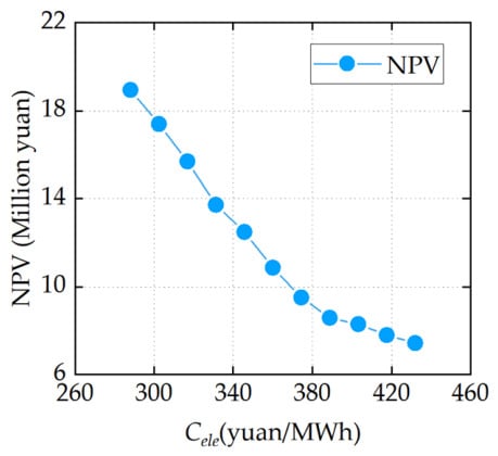
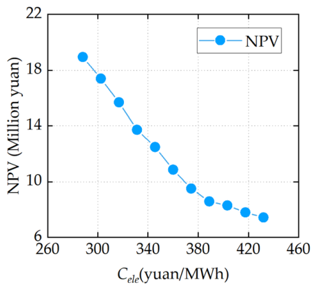
To assess the influence of the electricity-price assumption on the life-cycle economic result, an additional one-factor sensitivity analysis was conducted for the Hebei long-distance district heating network. The fixed electricity price was varied from 288 to 432 yuan/MWh, corresponding to −20% to +20% relative to the reference value of 360 yuan/MWh, with a 4-percentage-point increment at each step. Other network, operating, and economic parameters were retained at their case values. As shown in Figure 17, the NPV decreases monotonically as the electricity price increases. At the reference electricity price, the NPV is 10.8621 million yuan. Over the tested range, the NPV decreases from approximately 18.9 million yuan to 7.4 million yuan but remains positive throughout. This result indicates that the bypass thermal storage scheme remains economically feasible within the investigated electricity-price range, although the absolute economic benefit is sensitive to the electricity-price level. The proposed framework can be reapplied with updated network and economic parameters to evaluate the corresponding bypass configuration and economic performance under different engineering conditions.
Figure 17.
Influence of the electricity-price assumption on the NPV.
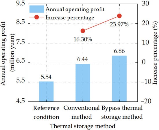
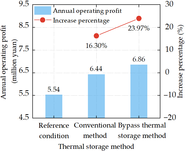
Figure 18 and Table 9 compare the two thermal storage methods in terms of annual operating profit and life-cycle economic performance, respectively. Annual operating profit is obtained by aggregating NBtotal over the annual evaluation period. For the electricity spot-market case considered here, NBtotal = NBop. As shown in Figure 18, the annual operating profits of the unit in the urban primary district heating network under the reference condition, the conventional district heating network thermal storage method, and the bypass thermal storage method are 5.54 million yuan, 6.44 million yuan, and 6.86 million yuan, respectively. The bypass thermal storage method yields the highest annual operating profit.
Figure 18.
Comparison of annual operating profit in the electricity spot market.
Table 9.
Life-cycle economic performance under different district heating network thermal storage methods.
Table 9 further shows that, with the conventional district heating network thermal storage method, the present values of incremental operating profit under peak- and valley-price conditions are 0.21 million yuan and 5.34 million yuan, respectively, resulting in an NPV of 5.54 million yuan. With the bypass thermal storage method, the corresponding present values increase to 0.30 million yuan and 7.85 million yuan, respectively, and the NPV reaches 8.02 million yuan, representing an increase of 44.70% over the conventional district heating network thermal storage method. These two sets of results corroborate each other, indicating that the bypass thermal storage method not only increases annual operating profit but also provides better life-cycle economic performance after the costs of the bypass devices are taken into account.
7. Conclusions
This study applies a bypass thermal storage method to exploit the thermal storage potential of a return-water network. It also develops a bilevel optimization model for CHP operation in an urban primary DHN and a long-distance DHN under different electricity-market mechanisms. The main conclusions are as follows:
- (1)
- When all typical heat-load and typical electricity-price scenarios are jointly incorporated into the optimization, thermal storage bypass devices do not need to be installed at every station. Appropriate installation at selected nodes can effectively utilize the thermal storage potential of the return-water pipe network, expand the electrical power adjustment range of combined heat and power units, and improve their operating economy. In the cases considered in this study, the bypass flow is concentrated mainly at intermediate and distant heating substations.
- (2)
- Under network thermal-release conditions, the combined heat and power units operate more economically. In the peak-shaving ancillary services market, the real-time heat-supply power of the heat source decreases, bringing the unit load ratio into the compensated peak-shaving range and thereby generating compensated peak-shaving power. In the electricity spot market, during the initial stage of thermal release, the units increase their electrical power output under peak-price conditions to increase electricity-generation revenue and reduce their electrical power output under valley-price conditions to reduce operating losses.
- (3)
- Compared with the conventional district heating network thermal storage method, the bypass thermal storage method yields a higher total operating profit. In the peak-shaving ancillary services market, the peak-shaving compensation revenue obtained using the conventional district heating network thermal storage method is insufficient to offset the reduction in unit operating profit. By contrast, the life-cycle NPV reaches 10.8621 million yuan when the bypass thermal storage method is adopted. In the electricity spot market, the life-cycle NPV obtained using the bypass thermal storage method is 44.70% higher than that obtained using the conventional district heating network thermal storage method.
This study provides an engineering basis for utilizing DHN thermal storage to enhance CHP operational flexibility and economic performance. The proposed optimization framework can be applied to other DHNs, with optimal bypass configurations and economic benefits depending on local engineering conditions and market rules. Future research will investigate bypass thermal storage and its economic optimization in DHNs integrating multiple types of heat sources, including renewable energy sources.
Author Contributions
L.R.: Writing—Original Draft, Visualization, Software, Data Curation. J.W.: Writing—Review and Editing, Supervision, Funding Acquisition, Conceptualization. J.G.: Methodology, Formal Analysis, Data Curation. X.G.: Software, Project Administration, Data Curation. C.Q.: Supervision, Project Administration, Conceptualization. All authors have read and agreed to the published version of the manuscript.
Funding
This study was supported by the National Natural Science Foundation of China (No. 52208104) and the Hebei Natural Science Foundation (No. E2024202065).
Data Availability Statement
The numerical model, input parameters, and anonymized measurement data supporting the findings of this study are available from the corresponding author upon reasonable request.
Acknowledgments
We would like to thank the Hebei Gongda Keya Group Co., Ltd. for providing the necessary data and field study platform. Jinda Wang is thankful for support from the Initial Research Funding of Hebei University of Technology.
Conflicts of Interest
Author Xiaoyu Gao was employed by the company Hebei Gongda Keya Energy Technology Co., Ltd. The remaining authors declare that the research was conducted in the absence of any commercial or financial relationships that could be construed as potential conflicts of interest.
Abbreviations
The following abbreviations are used in this manuscript:
| ARI | Adjusted Rand index | NPV | Net present value |
| CHP | Combined heat and power | WCSS | Within-cluster sum of squares |
| DHN | District heating network | ||
| Cb,reform | Retrofit cost of the thermal storage bypasses, yuan | QCHPele,equ | Equivalent electrical output under condensing-only operation, MW |
| Cb,total | Total life-cycle cost of the bypasses, yuan | QCHPele,max | Maximum electrical output under condensing-only operation, MW |
| Cele | Electricity price, yuan/MWh | QCHPinput | Input power of the unit, MW |
| Cfuel | Fuel cost per unit of lower heating value, yuan/MWh | Qex | Heat exchange power, MW |
| Cib,others | Cost of other materials and associated construction, yuan | Qp | Pump power, MW |
| Cib,pipe | Bypass-pipe cost, yuan | Qsc,hr | Thermal output of the heat source under the thermal-release condition, MW |
| Cib,val | Bypass-valve cost, yuan | r | Annual interest rate |
| Cth | Heat-selling price, yuan/MWh | RaT,s | Maximum permissible ramp rate of the heat-source supply temperature, °C/h |
| cw | Specific heat capacity, kJ/(kg·°C) | T scr,hr | Return-water temperature at the heat source under the thermal-release condition, °C |
| D | Diameter, m | T scs,ref | Reference supply water temperature at the heat source, °C |
| Ehs | Total stored thermal energy, GJ | Tr | Return-water temperature, °C |
| FCfuel | Coal consumption coefficient | Ts | Supply-water temperature, °C |
| Gb | Bypass flow rate, t/h | Ts,hs | Supply temperature under the thermal storage condition, °C |
| Gex | Heat exchange flow rate, t/h | Tscs,max | Maximum heat-source supply temperature, °C |
| Gsc,hr | Total circulating flow rate at the heat source under the thermal-release condition, t/h | V | Volume, m3 |
| NBop | Operating profit of the unit, yuan | y | Number of years in the analysis period |
| NBps | Peak-shaving ancillary service revenue, yuan | αBC,1 | Slope of the back-pressure operating line BC |
| NBtotal | Total operating profit of the unit, yuan | ΔNBay | Annual aggregate operating-profit increment, yuan |
| NPV | Net present value, yuan | ΔQth,hr | Reduction in the thermal output, MW |
| NRMSE | Normalized root-mean-square error, % | ζ | Specific electrical power loss |
| Numb | Number of bypass installations | ηCHPele | Overall electrical efficiency |
| OBJ | Objective function | θele | Actual electrical load ratio |
| pk | Representative weight of the k-th typical electricity-price profile | θele,equ | Equivalent electrical load ratio |
| pu | Representative weight of the u-th typical heat-load scenario | θele,ps | Reference load ratio for peak-shaving compensation |
| PVAF | Present value annuity factor | ρw | Density of water, kg/m3 |
| QCHPele | Electrical power output, MW | τ | Time, h |
References
- Guerra, K.; Haro, P.; Gutiérrez, R.E.; Gómez-Barea, A. Facing the high share of variable renewable energy in the power system: Flexibility and stability requirements. Appl. Energy 2022, 310, 118561. [Google Scholar] [CrossRef] [Scilit]
- Clean Heating Industry Committee, China Association of Small and Medium Enterprises. China Clean Heating Industry Development Report (2025); Clean Heating Industry Committee, China Association of Small and Medium Enterprises: Beijing, China, 2025. [Google Scholar]
- Liu, M.; Ma, G.F.; Wang, S.; Wang, Y.; Yan, J.J. Thermo-economic comparison of heat–power decoupling technologies for combined heat and power plants when participating in a power-balancing service in an energy hub. Renew. Sustain. Energy Rev. 2021, 152, 111715. [Google Scholar] [CrossRef] [Scilit]
- Guelpa, E.; Verda, V. Thermal energy storage in district heating and cooling systems: A review. Appl. Energy 2019, 252, 113474. [Google Scholar] [CrossRef] [Scilit]
- Pans, M.A.; Eames, P.C. A study of the benefits of including thermal energy stores in district heating networks. Renew. Energy 2024, 231, 120887. [Google Scholar] [CrossRef] [Scilit]
- Wang, L.Y.; Zhang, S.Q.; Fu, Y.; Liu, M.; Liu, J.P.; Yan, J.J. Usable thermal energy stored in the district heating system for peak shaving: A dynamic simulation study. Appl. Therm. Eng. 2024, 239, 122169. [Google Scholar] [CrossRef] [Scilit]
- Chen, Q.; Meng, N.; He, K.L.; Ma, H.; Gou, X. Multi-time scale operation optimization of integrated power and thermal system considering load disturbance. Energy 2024, 302, 131935. [Google Scholar] [CrossRef] [Scilit]
- Wang, H.; Meng, H. Improved thermal transient modeling with new 3-order numerical solution for a district heating network with consideration of the pipe wall’s thermal inertia. Energy 2018, 160, 171–183. [Google Scholar] [CrossRef] [Scilit]
- Meibodi, S.S.; Rees, S.; Loveridge, F. Modeling district heating pipelines using a hybrid dynamic thermal network approach. Energy 2024, 290, 130107. [Google Scholar] [CrossRef] [Scilit]
- Xie, Z.C.; Wang, H.C.; Hua, P.M.; Lahdelma, R. Discrete event simulation for dynamic thermal modelling of district heating pipe. Energy 2023, 285, 129523. [Google Scholar] [CrossRef] [Scilit]
- Van Oevelen, T.; Scapino, L.; Al Koussa, J.; Vanhoudt, D. A case study on using district heating network flexibility for thermal load shifting. Energy Rep. 2021, 7, 1–8. [Google Scholar] [CrossRef] [Scilit]
- Kuosa, M.; Kiviranta, P.; Sarvelainen, H.; Tuliniemi, E.; Korpela, T.; Tallinen, K.; Koponen, H.K. Optimisation of district heating production by utilising the storage capacity of a district heating network on the basis of weather forecasts. Results Eng. 2022, 13, 100318. [Google Scholar] [CrossRef] [Scilit]
- Kouhia, M.; Laukkanen, T.; Holmberg, H.; Ahtila, P. District heat network as a short-term energy storage. Energy 2019, 177, 293–303. [Google Scholar] [CrossRef] [Scilit]
- Nigro, L.; La Bella, A.; Casella, F.; Scattolini, R. Control-oriented modeling, simulation, and predictive control of district heating networks. IEEE Trans. Autom. Sci. Eng. 2025, 22, 7064–7079. [Google Scholar] [CrossRef] [Scilit]
- Zheng, J.F.; Zhou, Z.G.; Zhao, J.N.; Wang, J.D. Integrated heat and power dispatch truly utilizing thermal inertia of district heating network for wind power integration. Appl. Energy 2018, 211, 865–874. [Google Scholar] [CrossRef] [Scilit]
- Garcet, J.; De Meulenaere, R.; Blondeau, J. Enabling flexible CHP operation for grid support by exploiting the DHN thermal inertia. Appl. Energy 2022, 316, 119056. [Google Scholar] [CrossRef] [Scilit]
- Liang, M.L.; Ji, J.; Gao, Y.H.; Li, F.Q. Theoretical and experimental research on utilizing thermal inertia of heating network to improve the regulating capacity of combined heat and power units. Energy Conserv. Technol. 2025, 43, 429–436. [Google Scholar]
- Zheng, J.F.; Zhou, Z.G.; Zhao, J.N.; Wang, J.D. Effects of the operation regulation modes of district heating system on an integrated heat and power dispatch system for wind power integration. Appl. Energy 2018, 230, 1126–1139. [Google Scholar] [CrossRef] [Scilit]
- Jiang, Y.B.; Wan, C.; Botterud, A.; Song, Y.H.; Xia, S.W. Exploiting flexibility of district heating networks in combined heat and power dispatch. IEEE Trans. Sustain. Energy 2020, 11, 2174–2188. [Google Scholar] [CrossRef] [Scilit]
- Gou, X.; Chen, Q.; He, K.L. Real-time quantification for dynamic heat storage characteristic of district heating system and its application in dispatch of integrated energy system. Energy 2022, 259, 124960. [Google Scholar] [CrossRef] [Scilit]
- Yang, M.; Ding, T.; Chang, X.Y.; Xue, Y.X.; Ge, H.C.; Jia, W.H.; Du, S.J.; Zhang, H.J. Analysis of equivalent energy storage for integrated electricity-heat system. Energy 2024, 303, 131892. [Google Scholar] [CrossRef] [Scilit]
- Hennessy, J.; Li, H.L.; Wallin, F.; Thorin, E. Flexibility in thermal grids: A review of short-term storage in district heating distribution networks. Energy Procedia 2019, 158, 2430–2434. [Google Scholar] [CrossRef] [Scilit]
- Rong, L.; Wang, J.; Gao, X.; Qi, C.; Wu, X. Dual-layer configuration optimization model of bypass branches for heat storage in district heating network. J. Energy Storage 2025, 118, 116197. [Google Scholar] [CrossRef] [Scilit]
- Li, Z.; Wu, W.; Shahidehpour, M.; Wang, J.; Zhang, B. Combined heat and power dispatch considering pipeline energy storage of district heating network. IEEE Trans. Sustain. Energy 2016, 7, 12–22. [Google Scholar] [CrossRef] [Scilit]
- Merkert, L.; Abdoul Haime, A.; Hohmann, S. Optimal scheduling of combined heat and power generation units using the thermal inertia of the connected district heating grid as energy storage. Energies 2019, 12, 266. [Google Scholar] [CrossRef] [Scilit]
- Lei, Q.; Chong, D.T.; Zhao, Q.B.; Wang, J.S. Dynamic simulation and thermodynamic analysis of energy storage in heat supply network. J. Eng. Thermophys. 2024, 45, 2965–2973. [Google Scholar]
- Huang, G.Q.; Huang, C.; Liu, H.; Huang, H.M.; Shang, W.T.; Wang, W.L. Exergy analysis of off-design performance in solar-aided power generation systems: Evaluating the rationality of using part-load operation solution of coal-fired plants. Energy 2024, 302, 131749. [Google Scholar] [CrossRef] [Scilit]
- Liu, F.G.; Li, S. Prediction of carbon emissions from coal-fired power plants during load cycling with varying coal characteristics. Fuels 2025, 6, 1. [Google Scholar] [CrossRef] [Scilit]
- Gadd, H.; Werner, S. Daily heat load variations in Swedish district heating systems. Appl. Energy 2013, 106, 47–55. [Google Scholar] [CrossRef] [Scilit]
- Guelpa, E.; Marincioni, L. Demand side management in district heating systems by innovative control. Energy 2019, 188, 116037. [Google Scholar] [CrossRef] [Scilit]
- CJJ 88-2014; Technical Specification for Operation and Maintenance of Urban Heating System. China Architecture & Building Press: Beijing, China, 2014.
- Xie, Z.C.; Wang, H.C.; Hua, P.M.; Lahdelma, R. Hydraulic–thermal dynamic model of meshed district heating network based on discrete event simulation. Energy 2025, 339, 138895. [Google Scholar] [CrossRef] [Scilit]
- Steinegger, J.; Wallner, S.; Greiml, M.; Kienberger, T. A new quasi-dynamic load flow calculation for district heating networks. Energy 2023, 266, 126410. [Google Scholar] [CrossRef] [Scilit]
- Xie, Z.C.; Wang, H.C.; Hua, P.M.; Björkstam, M.; Lahdelma, R. Dynamic thermal simulation of a tree-shaped district heating network based on discrete event simulation. Energy 2024, 313, 133775. [Google Scholar] [CrossRef] [Scilit]

Disclaimer/Publisher’s Note: The statements, opinions and data contained in all publications are solely those of the individual author(s) and contributor(s) and not of MDPI and/or the editor(s). MDPI and/or the editor(s) disclaim responsibility for any injury to people or property resulting from any ideas, methods, instructions or products referred to in the content. |
© 2026 by the authors. Licensee MDPI, Basel, Switzerland. This article is an open access article distributed under the terms and conditions of the Creative Commons Attribution (CC BY) license.