


Abstract
This study examines the feasibility of combining Sparse Identification of Nonlinear Dynamical Systems (SINDy)-based data augmentation with an Actor–Critic deep reinforcement learning (DRL) model in a dataset-driven exploratory policy-learning configuration under limited-data conditions. The modeling and training dataset comprised 511 observations collected at 10-min intervals during the first seven days of an eight-day monitoring campaign; 10 conditions from the eighth day were reserved exclusively for decision evaluation. The SINDy equations were identified using 73 observations from one selected day, while the first measured observation of each day was subsequently used to initialize seven daily simulations, producing a 511-point augmented dataset. DRL models trained on the original, SINDy-augmented, and interpolation-augmented datasets were compared. Across the six modeled variables, descriptive trajectory-reconstruction R2 values obtained under the investigated data configuration ranged from 0.6446 to 0.8126. In a small descriptive comparison of 10 test conditions, the models trained on the original and SINDy-augmented datasets each showed complete-action agreement with the participant-derived recommendations in 7 of 10 cases, whereas the interpolation-augmented model achieved no complete-action agreements. These results support the feasibility of the framework under the investigated dormitory conditions. Further validation is required because the study involved a single building, a short monitoring period, one training run per dataset, and a small decision test set.
1. Introduction
Maintaining optimal indoor thermal comfort is crucial for enhancing the well-being and productivity of occupants [1,2]. It significantly impacts health, mood, and overall satisfaction with the living environment [3,4]. In living spaces where individuals rest and sleep, achieving the right balance of temperature and humidity is essential for fostering a conducive environment for relaxation and well-being. Traditionally, maintaining indoor thermal comfort has involved the use of heating, ventilation, and air conditioning (HVAC) systems that operate based on preset conditions and extensive manual adjustments [5,6,7]. These systems rely on static schedules and setpoints to regulate temperature, which can be inefficient and costly. Such approaches tend to overlook dynamic changes in occupancy and individual preferences, leading to suboptimal comfort levels and excessive energy consumption.
The rise of artificial intelligence (AI) has brought significant advancements in maintaining indoor thermal comfort [8,9]. AI technologies enable the development of more adaptive and intelligent systems that can respond to real-time conditions and occupant behaviors [10,11]. By leveraging AI, these systems can learn from past data and make predictions to optimize climate control strategies, thereby enhancing both comfort and energy efficiency [12,13]. Moon et al. [14] developed an artificial neural network (ANN) model to predict the optimal time for adjusting setback temperatures within buildings during normal occupancy periods. They also introduced an algorithm that uses this ANN model to enhance indoor thermal comfort and boost building energy efficiency. Wang et al. [15] used AI-powered cameras and deep vision algorithms to monitor occupant behavior and window usage in a building, developed predictive models to understand its responses, and introduced a strategy to enhance indoor comfort, energy efficiency, and air quality.
While existing artificial intelligence approaches have achieved satisfactory performance in predicting indoor thermal conditions and occupants’ comfort responses, their ability to provide adaptive control remains limited. As an important branch of artificial intelligence, deep reinforcement learning (DRL) offers a promising alternative by enabling real-time interaction with the environment and continuous optimization of control actions. Through dynamically adjusting indoor environmental parameters according to changing occupancy patterns and environmental conditions, DRL can simultaneously enhance thermal comfort and energy efficiency [16]. DRL algorithms can learn optimal control strategies through interaction with the environment, allowing for continuous adaptation to changing conditions and occupant behaviors [17]. This approach has the potential to significantly improve energy efficiency while maintaining or enhancing thermal comfort. Yu et al. [18] developed a control algorithm using Deep Q-Learning in reinforcement learning to optimize the energy consumption of air-conditioning and exhaust fans. Their algorithm effectively balances indoor air quality (CO2 levels), thermal comfort, and energy usage. Valladares et al. [19] proposed an artificial intelligence algorithm designed to maintain optimal thermal comfort and air quality with minimal energy consumption from air-conditioning units and ventilation fans.
Although DRL has demonstrated remarkable effectiveness in optimizing complex systems and enabling adaptive indoor environmental control, its practical deployment remains constrained by the substantial amount of training data required for policy learning [20]. Effective DRL training typically relies on large volumes of high-quality data collected over extended periods, which can be costly and time-consuming to obtain in real building environments [21]. This demand for significant data collection impedes the practical application and scalability of DRL, particularly in residential settings where such data may not be easily obtainable. Furthermore, the training processes of DRL models often exhibit a “black-box” effect [22], obscuring the decision-making process and making it difficult to understand how decisions are made, which complicates trust and interpretability in real-world applications.
This paper proposes a framework that integrates Sparse Identification of Nonlinear Dynamical Systems (SINDy) [23] with Deep Reinforcement Learning (DRL) to address the challenges of data limitations. SINDy allows for the identification of sparse dynamic relationships between variables from limited measured observations. In our research, we use a university student dormitory as the case study. By utilizing SINDy, additional training trajectories can be generated from a model identified using one day of measurements, together with measured daily initial conditions. These augmented trajectories are subsequently used to examine the feasibility of DRL training under the investigated limited-data configuration. Additionally, the explicit equations identified by SINDy provide an interpretable representation of the modeled environmental dynamics and the data-augmentation process. This added transparency applies primarily to the SINDy-based data-generation stage rather than to the internal decision-making mechanism of the DRL policy, which remains neural-network based.
Unlike conventional model-based reinforcement learning, in which a transition model is primarily constructed for planning or policy optimization, the present framework uses SINDy mainly as an interpretable data-augmentation mechanism for subsequent DRL training. Physics-informed machine-learning approaches generally incorporate predefined physical laws or constraints, whereas the present method identifies sparse dynamic relationships directly from measured data. Similarly, calibrated digital twins aim to reproduce building behavior with relatively high physical fidelity, while generic surrogate models mainly emphasize predictive approximation. In contrast, the proposed framework focuses on obtaining explicit sparse equations from limited observations and using these equations to generate additional training data. Accordingly, the main contributions of this study are: (1) integrating SINDy-based data augmentation with DRL under limited-data conditions; (2) providing explicit and interpretable dynamic equations for the augmented variables; and (3) comparatively evaluating original, interpolation-augmented, and SINDy-augmented datasets in DRL training. Compared with conventional prediction-oriented approaches, the proposed framework focuses on generating additional training trajectories from limited measured data while retaining explicit dynamic relationships for subsequent exploratory DRL policy analysis.
2. Related Works
2.1. Artificial Intelligence in Indoor Thermal Comfort
Indoor thermal comfort is crucial for the well-being, productivity, and health of occupants, as people spend a considerable amount of time indoors [24,25]. Effective management of the indoor thermal environment is essential to ensure occupant satisfaction and overall health. Traditional Heating, Ventilation, and Air Conditioning (HVAC) systems are engineered to regulate indoor climates using preset environmental conditions and manual controls [26]. These systems commonly operate on static schedules and thermostat setpoints, adjusted for average occupancy and environmental conditions [27,28]. This approach lacks the flexibility to respond to actual changes in building occupancy or environmental variables, leading to inefficiencies in maintaining real-time indoor comfort. The integration of Artificial Intelligence (AI) technologies into HVAC systems has significantly improved their adaptability and intelligence [29]. Utilizing Artificial Neural Networks (ANN) and deep learning models, these AI-enhanced systems efficiently process real-time data from sensors monitoring temperature, humidity, CO2 levels, and occupancy [30,31]. This capability enables HVAC systems to dynamically adjust their operations, not only improving comfort levels but also minimizing energy consumption [32,33]. The real-time adaptation ensures that environmental conditions are consistently aligned with the current needs of the building’s occupants.
Artificial intelligence has demonstrated significant potential in indoor thermal management due to its capability to learn complex relationships between environmental variables and occupants’ thermal comfort responses. Kim et al. [34] found that personal comfort models based on individual heating and cooling behaviors can accurately predict thermal preferences. Thus, these models can be effectively utilized in daily comfort management to enhance occupant satisfaction and optimize energy consumption in buildings [35,36,37]. Hamdi and Lachiver [38] developed a concept of comfort conditions based on human sensitivity, focusing not on maintaining a constant internal temperature but on sustaining consistent indoor comfort levels. Their findings suggest that it is possible to balance occupant comfort while conservatively managing resources. By continuously analyzing data, AI can customize environmental settings to suit the individual preferences of each occupant, enhancing occupant satisfaction [39]. This personalized approach is powered by machine learning algorithms that adapt to occupants’ daily patterns and preferences, optimizing both comfort and energy efficiency [40]. By analyzing historical data and environmental conditions, AI algorithms can anticipate potential system failures before they manifest [41,42]. This proactive approach not only reduces the likelihood of breakdowns but also lowers maintenance costs and decreases system downtime, thereby ensuring uninterrupted comfort for all building occupants.
To achieve these functions, a variety of machine learning algorithms have been adopted in indoor thermal management research. Table 1 summarizes the characteristics and representative applications of commonly used machine learning methods.
Table 1.
Summary of machine learning algorithms in indoor thermal management.
As shown in Table 1, existing machine learning approaches have been widely applied to thermal comfort prediction, environmental assessment, and personalized thermal management. However, most of these methods focus primarily on predictive tasks and provide limited support for adaptive control under dynamically changing indoor conditions.
In comparison, simpler methods such as linear regression and decision trees generally offer lower computational cost and greater interpretability, whereas ensemble and nonlinear methods can capture more complex relationships but usually require more data and provide less transparent model structures. These trade-offs limit the ability of conventional machine-learning approaches to simultaneously achieve low data demand, model interpretability, and adaptive real-time control.
2.2. Deep Reinforcement Learning in Thermal Comfort Management
Reinforcement Learning (RL) is a sophisticated AI methodology that enables systems to make autonomous, data-driven decisions by learning from interactions with their environment [51]. In the field of indoor thermal comfort, RL is applied to enhance the operation of Heating, Ventilation, and Air Conditioning (HVAC) systems. RL models process variables like indoor and outdoor temperatures, humidity, and occupant preferences, and adjust settings dynamically to achieve optimal comfort [52]. Excelling in environments that demand adaptability, RL is pivotal for effective thermal management. Table 2 shows the most common reinforcement learning algorithms and their applications in the thermal engineering field.
Building on the foundations of RL, Deep Reinforcement Learning (DRL) incorporates deep learning techniques, allowing it to handle more complex data sets and provide more sophisticated solutions. DRL integrates the core principles of reinforcement learning with the powerful data-processing capabilities of deep neural networks [53]. This combination enables DRL models to process intricate variables and interactions within HVAC systems, improving the precision and effectiveness of comfort adjustments. The use of DRL in conjunction with Internet of Things (IoT) devices has also propelled the advancement of smart homes [54,55], where systems autonomously adjust temperature and humidity based on real-time environmental data and user preferences. The enhanced complexity and capability of DRL make it particularly suitable for navigating the multifaceted dynamics of modern thermal environments, showcasing its substantial potential in practical, real-world applications.
However, DRL often requires substantial training data and provides limited transparency regarding its internal decision process. To address the data-demand issue, the present study integrates Sparse Identification of Nonlinear Dynamical Systems (SINDy) with DRL. SINDy identifies sparse dynamic relationships from measured observations and generates additional trajectories for subsequent DRL training. More importantly, its explicit equations provide a transparent representation of the modeled environmental dynamics and the data-generation process. This interpretability applies to the SINDy-based augmentation stage, while the Actor–Critic policy itself remains a neural-network-based decision model.
Table 2.
The reinforcement learning algorithms and their applications in the thermal engineering field.
As summarized in Table 2, conventional tabular RL methods such as Q-learning and SARSA are relatively interpretable and computationally simple, but their applicability decreases as the state–action space becomes more complex. Deep RL methods, including DQN, policy-gradient, and Actor–Critic approaches, provide greater flexibility for high-dimensional control problems but generally require more training data and computational resources and offer lower interpretability. This comparison motivates the integration of SINDy with DRL in the present study, using model-based data augmentation to generate additional training trajectories from limited measurements while retaining explicit dynamic relationships.
3. Methods
This section first presents the overall workflow (Section 3.1), followed by data collection (Section 3.2), SINDy model identification and data augmentation (Section 3.3), and Actor–Critic DRL training (Section 3.4).
3.1. Overview of the Method
The proposed workflow comprises data collection, SINDy model identification, SINDy-based data augmentation, and DRL training, as summarized in Figure 1.
Figure 1.
Overview of the proposed method.
3.2. Data Collection and Experimental Protocol
The field study comprised an eight-day monitoring campaign conducted in a university student dormitory in Beijing during early summer. Measurements were collected from 8:00 A.M. to 8:00 P.M. at 10-min intervals during the first seven consecutive days, providing 73 observations per day and 511 observations in total. These 511 observations formed the model-development and DRL-training pool; within this pool, 73 observations from one selected day were used for SINDy identification, and the first measured observation of each of the seven days was used to initialize the corresponding daily simulation. Measurements from an eighth monitoring day were reserved exclusively for decision evaluation and were not used in any model-identification, augmentation, or training step. The dataset included outdoor temperature and relative humidity, indoor temperature and relative humidity, indoor air velocity, and the operational states of the window, door, and air conditioner. Outdoor temperature data were obtained from the National Meteorological Information Center of the China Meteorological Administration (http://data.cma.cn).
Figure 2 shows the instruments used for environmental measurements. Indoor air velocity was measured using a handheld vane anemometer (Delixi) with a measurement range of 0.3–30 m/s and a manufacturer-specified error of ±5%. Temperature and relative humidity were measured using temperature–humidity gauges with measurement ranges of −50–110 °C and 10–90% RH and manufacturer-specified errors of ±1 °C and ±5%, respectively. Indoor temperature, relative humidity, and air velocity were measured at the fixed location shown in Figure 3, at 1.1 m above floor level. The vane anemometer measured local air velocity at this point and was not an omnidirectional three-dimensional airflow sensor; therefore, the measurements should not be interpreted as a complete characterization of the indoor airflow field.
Figure 2.
Environmental measurement instruments and their main measurement specifications.
Figure 3.
Floor plan and environmental measurement locations. Indoor temperature, relative humidity, and air velocity were measured at the indicated location at 1.1 m above floor level.
Six students participated in the experiment and independently reported their thermal sensation at each measurement interval. Because no cold sensations were reported during the summer monitoring period, responses were recorded on a scale from 0 (thermally neutral) to 5 (very hot), with 0.5-point increments. Participants engaged in light activities such as reading or listening to music and avoided strenuous activity. They remained in the room during lunch and consumed pre-prepared meals to minimize disruption, while lightweight long-sleeve shirts and pants were used to reduce major variation in clothing conditions. Activity and clothing were therefore controlled qualitatively, but metabolic rate and clothing insulation were not quantified in met and clo units. Mean radiant temperature was also not independently measured; consequently, PMV and PPD according to ISO 7730 were not calculated. The present study therefore evaluates occupant-reported thermal sensation rather than a complete standards-based thermal-comfort assessment. Basic participant information is provided in Table 3.
Table 3.
Participant’s basic information.
To support consistent reporting over the 12-h monitoring period, participants were reminded every 10 min using a digital timer, and periodic checks were conducted by the research team. The completed score sheets contained no missing entries or unusual repetition patterns. For each time step, the most frequently selected thermal sensation score was adopted as the representative group response; when two or more scores were equally frequent, the mean of the tied values was used. This mode-based aggregation with mean tie-breaking provides a simple group-level response for subsequent modeling, although it does not preserve the full distribution of individual responses. Alternative aggregation approaches should therefore be considered in future studies.
Figure 4 shows the outdoor and indoor temperature and humidity for the third day of the week. From this picture, we can see that the outdoor temperature steadily increases until mid-afternoon before declining, while the indoor temperature experiences less fluctuation. The outdoor humidity decreases significantly during the afternoon and then rises towards the evening, whereas the indoor humidity remains relatively stable throughout the day. The inconsistency in fluctuations between indoor and outdoor temperatures can be attributed to the regulation provided by air conditioning.
Figure 4.
Indoor and outdoor temperature and humidity charts. (a) Outdoor and indoor temperature over time; (b) outdoor and indoor humidity over time.
Figure 5 displays a correlation matrix illustrating the relationships among various environmental and subjective factors: Outdoor Temperature, Outdoor Humidity, Indoor Temperature, Indoor Humidity, Wind Speed, Air Conditioning Status (AC Status), and Thermal Sensation Score. Each cell in the matrix shows the computed Pearson correlation coefficient (r-value). From this figure, we observe a strong negative correlation between Outdoor Temperature and Outdoor Humidity (r = −0.93), as well as a strong positive correlation between Indoor Temperature and Thermal Sensation Score (r = 0.72).
Figure 5.
Correlation matrix of various environmental performance parameters.
3.3. The Process of Training the SINDy Model and Data Expansion
3.3.1. Introduction to Sparse Identification of Nonlinear Dynamical Systems (SINDy)
Sparse dictionary learning techniques represent a type of symbolic regression utilized for revealing interpretable representations of nonlinear functions from available data. Unlike some symbolic regression algorithms that employ evolutionary or genetic algorithms to generate functions through combinations of candidate library functions and mathematical operations, dictionary learning algorithms approximate functions solely as linear combinations of candidate “dictionary” functions. This approach enables efficient fitting using traditional linear regression methods, in contrast to the computationally expensive nature of gradient-free algorithms typically utilized in symbolic regression.
The SINDy algorithm employs sparse dictionary learning to unveil the governing equations of dynamical systems. Initially, we outline a comprehensive formulation of sparse dictionary learning before establishing its relevance to various dynamics discovery frameworks. It utilizes sparse representation learning techniques to infer the system’s differential equations by observing the system’s evolution and sampling its states. The fundamental idea is to represent the system’s evolution as a linear combination of a set of basis functions and employ a sparse coefficient matrix to capture the nonlinear dynamical characteristics of the system. The mathematical formulation of SINDy can be expressed as follows:
Consider a dynamical system described by
where represents the system’s state at time and describes its dynamics. Data is represented in matrices and constructed from state vectors at sampled times (Equation (2)):
A function library matrix includes candidate functions like constants, polynomials, and trigonometric functions:
The goal is to approximate by a sparse combination of these functions, formulated as
where are coefficients optimized to fit the data while promoting sparsity:
This results in a compact model that efficiently captures the system dynamics using fewer terms, enhancing both interpretability and computational performance.
3.3.2. The Method of Training the SINDy Model and Expanding the Dataset
The original dataset comprises 511 observations collected at 10-min intervals over seven days. To examine the proposed augmentation under limited identification data, the SINDy equations were fitted using 73 observations from one selected day. The remaining six days were not used to fit the equations; however, the first measured observation from each of the seven days was subsequently used to initialize the daily simulations. Thus, the study evaluates one-day model identification with measured daily initial conditions, rather than data generation based exclusively on a single day.
In the process of training the SINDy model and data expansion (Figure 6), we define the time index (T) as a numerical representation of time within a day. Each time point is assigned a unique integer from 1 to 73, representing the sequence of these intervals throughout the day. This time index serves as the control variable, capturing the temporal progression and serving as a basis for modeling the dynamics of continuous variables.
Figure 6.
Workflow of SINDy-based data augmentation. SINDy models were identified using 73 observations from one selected day. Seven measured daily initial conditions were used to generate 511 simulated samples, while door, window, and AC states were randomly sampled as exploratory control inputs.
In our dataset, the variables exhibit mutual influences, reflecting their interdependencies within the observed system. However, Outdoor Temperature and Outdoor Humidity are modeled as independent variables influenced solely by the time index because, in this dataset, no other variables directly impact them.
Although both outdoor temperature and outdoor relative humidity were modeled solely as functions of time, this assumption is valid within the context of our experiment, which was conducted over a continuous seven-day period with stable and sunny weather conditions. Under such circumstances, these outdoor parameters exhibit relatively consistent diurnal patterns that can be effectively captured using time-dependent dynamics.
We acknowledge that in more general settings, outdoor temperature and humidity may fluctuate due to sudden weather changes such as cloud cover, precipitation, or wind. However, such external disturbances did not occur during our data collection period and are therefore beyond the scope of the current modeling framework. Importantly, the SINDy approach remains flexible and can be retrained to capture the corresponding time-dependent behaviors under different weather scenarios, should such data be available.
The SINDy models were fitted using 73 observations collected on one selected day. After model fitting, seven daily trajectories were generated, with each trajectory containing 73 time steps. The first measured observation from each of the seven days was used only as the initial condition for the corresponding daily simulation. The seven simulated trajectories therefore produced a total of 511 generated observations. Thus, the study uses one day of data for SINDy model identification, together with seven measured daily initial conditions for subsequent simulation. This approach ensures a direct comparison between the original and simulated data. The same method is applied to other variables. For each simulated daily trajectory, the door, window, and air-conditioning states were randomly sampled to provide exploratory operating-state inputs for data augmentation. These randomly generated sequences were not intended to reproduce actual occupant behavior. In real buildings, these actions may depend on indoor and outdoor conditions, occupancy, previous actions, and individual preferences. Consequently, the generated operating-state sequences may include combinations that are uncommon in actual buildings, and the resulting augmented dataset should be interpreted as an exploratory dataset rather than a behaviorally validated representation of building operation. Future work should incorporate stochastic, Markov-based, or data-driven occupant-behavior models to generate more realistic operating sequences.
- (1)
- Outdoor Temperature and Humidity Model
Variable Definition:
where and represent the outdoor temperature and humidity, respectively.
Dynamics Equation Training:
This equation is trained based on time variation and outdoor temperature and humidity data.
Data Generation:
This equation is used to predict the future states of outdoor temperature and humidity using the trained dynamics equation. For N different initial states . The model simulates each scenario to generate data expanded by a factor of N.
- (2)
- Door Status, Window Status, and AC Status
Door Status, Window Status, and AC Status are treated as state variables and can be directly expanded by a factor of N using random methods.
Further, with AC Status and the outdoor variables as control variables, Indoor Temperature (°C) and Indoor Humidity (%) are considered as responsive state variables . Another set of equations is trained using the SINDy model. Based on the initial indoor conditions Xin(0) and control inputs, we can simulate and generate data expanded by N + 1.
- (3)
- Indoor Temperature and Humidity Model
Control variables:
where A is the AC Status and is the outdoor conditions.
Control variables are typically inputs that a user might manipulate to achieve desired behaviors in a dynamical system.
State variable:
Dynamics equation training:
Data generation:
- (4)
- Wind Speed Model
Wind Speed (Ws) is primarily influenced by the status of doors and windows and can be simulated to generate data expanded by N + 1 using the corresponding SINDy equations based on the enhanced state Xstate.
Control variable:
where A is the AC Status, W is the Window Status, and D is the Door Status.
Wind speed variable:
Dynamics equation training:
Data generation:
- (5)
- Thermal Sensation Score Model
Control variables:
State variable:
Dynamics equation training:
Data generation:
3.3.3. Training the SINDy Model and Expanding the Dataset
We used the outdoor temperature and humidity model to demonstrate how to use the data to train the SINDy model. In using the SINDy model to fit the data, several hyperparameters require careful tuning to achieve a balance between model complexity and accuracy. These include the polynomial degree, which controls the ability of the model to capture nonlinear dynamics; the sparsity threshold, which determines the complexity of the resulting equations; and the choice of feature libraries, which should align with the physical characteristics of the system. No additional normalization or standardization was applied before SINDy identification; the variables were retained in their recorded physical units. The same recorded variable scales were retained for the DRL input states.
We can use visualization techniques to select appropriate hyperparameters. Taking outdoor temperature data as an example, Figure 7 illustrates the impact of choosing different polynomial degrees on the SINDy model’s performance for outdoor temperature simulation. A polynomial degree of 1 oversimplifies the system’s dynamics, failing to capture the nonlinear relationships present in the data, which leads to significant deviations from the original trend. In contrast, a polynomial degree of 2 better captures the nonlinear interactions between variables, resulting in a simulated curve that closely aligns with the original data.
Figure 7.
Comparison of measured outdoor temperature and SINDy simulations using polynomial degrees 1 and 2.
Therefore, in this dataset, constructing the SINDy model for analyzing outdoor temperature and humidity data involves selecting polynomial terms up to the second degree. This choice effectively models the nonlinear interactions between temperature and humidity. Similarly, other hyperparameters can also be determined using this approach (Table 4).
Table 4.
Hyperparameters used in the SINDy model for modeling outdoor temperature and humidity.
Polynomial degrees of 1 and 2 were compared visually for the outdoor-temperature model, and degree 2 was adopted for the subsequent analysis. SR3 was used as the sparse optimizer, with a sparsity threshold of 0.01 and a relaxation parameter of ν = 10−5. A systematic sensitivity analysis covering additional polynomial degrees, sparsity thresholds, and measurement-noise levels was not conducted. Therefore, parameter stability and robustness to measurement noise are not claimed in the present study.
After training the SINDy model, dynamic equations describing the evolution of the outdoor environmental variables were obtained. The variables and represent outdoor temperature and outdoor humidity, respectively, while denotes the time index ranging from 1 to 73, corresponding to the 73 observations collected during a single day.
The equations are given by
Outdoor temperature (): .
Outdoor humidity (): .
To assess the trajectory-reconstruction performance of these two models, we conducted simulations starting from initial conditions derived from actual data. Figure 8 displays line plots for both the simulated and original data. It reveals consistent trends between the two datasets, although they do not perfectly align. The trajectories reproduce the main temporal trends while retaining reconstruction error; therefore, they should be interpreted as model-based approximations rather than replicas of the measurements.
Figure 8.
Comparison between the measured and SINDy-simulated outdoor variables: (a) outdoor temperature; (b) outdoor relative humidity.
Then, we can choose another set of X_out(0) to simulate additional data. We select the first data point of each day from the original one-week dataset as the new initial condition for X_out(0), which are as follows:
New X_out = np.array(
[[23.8,38,0], [24.8,40,0], [25.3,42,0], [26,44,0],
[22.3,44,0], [26.2,43,0], [25.5,42,0]]
)
# These 7 initials are the first data point of each day from the original one-week dataset.
After simulating these seven initial values, the generated trajectories are presented in Figure 9. Using this method, we can also simulate other variables such as Indoor Temperature, Indoor Humidity, Wind Speed, and Thermal Sensation Score. The statuses of the air conditioning, doors, and windows are randomly generated. For indoor temperature and indoor humidity, we provide seven initial values . These data points are also the first data point of each day from the original one-week dataset.
New X_in = np.array(
[[25.5,42], [25.6,41], [25.7,42], [27,42],
[25.3,44], [27.2,45], [27.5,43]]
)
# These 7 initials are the first data point of each day from the original one-week dataset.
Figure 9.
Raw SINDy-generated trajectories. The thermal-sensation panel shows unconstrained model outputs; values outside the observed 0–5 scale indicate extrapolation and are not interpreted as valid participant ratings.
The equations are as follows:
Indoor temperature: .
Indoor humidity: .
Here, x0 represents the indoor temperature, x1 represents the indoor humidity, u0 represents the outdoor temperature, u1 represents the outdoor humidity, and u2 represents the AC status.
For wind speed, the dynamical equation is
Here, x0 represents the wind speed, u0 represents the door status, and u1 represents the window status.
For the thermal sensation score, the dynamical equation is
Here, x0 represents the thermal sensation score, u0 represents the indoor temperature, u1 represents the indoor humidity, u2 represents the wind speed, and u3 represents the AC status.
Figure 9 shows the trajectories generated by the SINDy models. Table 5 reports R2 and MSE calculated between the 511-point generated series and the corresponding measured series. The SINDy equations were identified using 73 observations from one day, while the first measured observation of each of the seven days was used to initialize the corresponding daily simulation. Because the comparison uses measured initial conditions and includes the day used for model identification, the reported metrics should be interpreted as descriptive trajectory-reconstruction measures rather than independent out-of-sample validation results.
Table 5.
Descriptive trajectory-reconstruction metrics between the SINDy-generated and measured trajectories.
Agreement varied across variables, with R2 values ranging from 0.6446 for the thermal sensation score to 0.8126 for outdoor temperature. These values provide a preliminary numerical assessment under the investigated data configuration but do not establish model robustness or the statistical fidelity of the generated data.
Residual analysis, temporal holdout validation, uncertainty analysis, and comparisons of higher-order statistical properties were not performed. The generated data are therefore used for an exploratory feasibility analysis, and their reliability requires further validation.
Because the SINDy equation is continuous and no ordinal boundary was imposed, some generated thermal sensation scores fall outside the observed 0–5 response scale. These values are unconstrained model outputs rather than valid participant ratings and indicate extrapolation beyond the measurement domain. This boundary violation should be considered when interpreting the subsequent DRL results.
3.4. Training the DRL Model
After data augmentation, each dataset was used to train an Actor–Critic agent in a dataset-driven exploratory configuration. At each step, the agent selected one of eight door, window, and air-conditioning combinations, and the reward combined thermal sensation with heuristic penalties for air-conditioner operation and open door/window states. Subsequent environmental observations were taken from the dataset rather than generated in response to the selected action; consequently, this setup does not represent closed-loop interaction with a building environment.
In the general reinforcement-learning formulation, an agent interacts with an environment through sequences of states st, actions at, and rewards rt over discrete time steps. The agent’s policy π maps states to actions, while the environment supplies the state-transition dynamics and reward function.
In that general formulation, the agent observes st, selects at according to π, receives rt, and then encounters st+1. The implementation used in this study differs in one important respect: st+1 was the following record in the fixed dataset and did not depend on at, as specified in the data and environment setup below.
The agent’s objective in reinforcement learning is to learn an optimal policy π* that maximizes the cumulative reward over time. This is often formalized using the notion of the expected return Gt, which is the sum of future rewards discounted by a factor γ:
where γ is the discount factor, 0 ≤ γ ≤ 1, determining the present value of future rewards. The goal of the agent is to find the policy π that maximizes the expected return:
Reinforcement learning algorithms seek to find such optimal policies through exploration of the state-action space and exploitation of learned knowledge.
- (1)
- Data and Environment Setup
Our environment consists of the following components:
State (State): Composed of outdoor temperature (Outdoor Temp), outdoor humidity (Outdoor Hum), indoor temperature (Indoor Temp), indoor humidity (Indoor Hum), and wind speed (Wind Speed).
Action (Action): Controls the opening and closing states of doors, windows, and air conditioning, encoded as 8 distinct actions (0–7), each representing a different combination of door, window, and AC settings.
Specifically, the encoding of action a is as follows:
This forms a 3-bit binary number, where each bit represents the status of the air conditioning, window, and door, respectively.
a = 0 (000): AC off, Window closed, Door closed;
a = 1 (001): AC on, Window closed, Door closed;
a = 2 (010): AC off, Window open, Door closed;
a = 3 (011): AC on, Window open, Door closed;
a = 4 (100): AC off, Window closed, Door open;
a = 5 (101): AC on, Window closed, Door open;
a = 6 (110): AC off, Window open, Door open;
a = 7 (111): AC on, Window open, Door open.
The SINDy-generated thermal sensation scores were retained in their unconstrained form during the exploratory DRL training and were not clipped, transformed, or removed before use. Thermal sensation was not included directly in the DRL state vector; instead, the generated thermal sensation score was used in the thermal-sensation component of the reward function. Consequently, SINDy outputs outside the experimentally observed 0–5 response range could result in reward magnitudes outside those associated with valid participant ratings. This treatment reflects the original computational implementation and is considered when interpreting the resulting learned action-selection policy.
The DRL comparison used each dataset as a sequential state trajectory. At time step t, the five environmental variables in the current record formed st, and the following record formed st+1. The agent’s selected action entered the reward through the air-conditioner and door/window penalty terms, while the environmental trajectory remained fixed by the dataset. The SINDy equations were used to generate the augmented dataset before DRL training rather than as an online action-dependent transition model. Accordingly, the reported training represents dataset-driven exploratory policy learning and not a closed-loop building-control simulation.
Reward: Based on the Thermal Sensation Score of the residents, with penalties applied for the use of air conditioning. If the air conditioning is turned on, or if it is used simultaneously with doors or windows being open, the reward value is reduced.
- (2)
- Reward Function
In reinforcement learning, the reward function evaluates the quality of each action taken, guiding the model to learn the optimal strategy. Our reward function takes into account the following factors:
Thermal sensation score;
Heuristic penalty associated with air-conditioner operation;
Constraints on door and window states when the air conditioner is on;
Thermal-Sensation Reward RTS.
The thermal-sensation reward is based on the thermal sensation score associated with the current time step, expressed as the negative absolute deviation from the neutral state:
Air-Conditioner Operation Penalty RAC
When the air conditioner is on, a heuristic penalty is applied:
Here, −1 is the fixed penalty used when the air conditioner is on. This heuristic term discourages air-conditioner operation and does not represent measured electrical energy consumption or monetary cost; electrical power and tariff data were not collected.
Constraints on Door and Window States When AC is On Rconstraints
If the air conditioner is on and either the door or the window is open, an additional heuristic penalty is applied to discourage this operational combination. This penalty is an operational heuristic rather than a measurement or estimate of electrical energy consumption, energy cost, or energy savings:
The total reward R is composed of the following parts:
where
RTS represents the reward based on the thermal sensation score;
RAC represents a heuristic penalty associated with air-conditioner operation;
Rconstraints represents the penalty for having the door or window open when the air conditioner is on.
In Equation (27), the implemented total reward is the sum of the thermal-sensation reward, the air-conditioner operation penalty, and the door/window constraint penalty.
The reward coefficients were selected heuristically for this exploratory study rather than calibrated from measured electrical energy consumption or derived from a formal multi-objective optimization procedure. The thermal-sensation component used a multiplier of 10, the air-conditioner operation penalty was −1, and the additional penalty for operating the air conditioner while a door or window was open was −10. Equation (27) therefore gives the implemented total reward as R = R_TS + R_AC + R_constraints. The same coefficients were applied to all three training datasets. No systematic sensitivity analysis was performed, so the learned policies may depend on this weighting.
- (3)
- Algorithm Logic
Initialization: Randomly initialize the parameters of the policy network.
Observe State: At time step t, use record t as the current state st.
Select Action: Select action at from the current policy π.
Advance Dataset and Receive Reward: Compute rt using at and the thermal-sensation value associated with the current record, then use the following record as st+1. The selected action does not modify st+1.
Store Experience: Store the transition (st, at, rt, st+1) in the replay buffer.
Learn and Update: Randomly sample experiences from the replay buffer and use them to update the policy network, minimizing the discrepancy between predicted and actual rewards.
Repeat Process: Repeat steps 2–6 until the learning termination criteria are met or a predefined number of iterations is reached.
Objective
Using the aforementioned reinforcement learning framework, the agent aims to learn a policy π* that maximizes the expected discounted return Gt.
Here, is the discount factor, used to balance the importance of immediate and future rewards. The objective is to find the policy that results in a thermal sensation score as close as possible to 0 (the neutral state) under the given constraints and penalties associated with the operation of doors, windows, and air conditioning.
- (4)
- Loss Function
Based on the Actor–Critic method, in our model, the loss function consists of the actor and critic.
Actor Loss Function
The actor loss aims to maximize the expected return by using the advantage function to adjust the policy.
where
is the policy probability of taking action at in state st.
is the advantage function, defined as .
Critic Loss Function
The critic loss aims to minimize the mean squared error between the predicted value and the actual return.
where
is the discounted return at time step t.
is the value predicted by the value network for state st.
Total Loss Function
The total loss function is a weighted sum of the actor and critic losses.
- (5)
- Hyperparameter Settings
The main implementation settings of the Actor–Critic model are summarized in Table 6 to improve the reproducibility of the DRL procedure. The model was trained using the Adam optimizer, with experiences stored in a replay buffer and randomly sampled during network updates.
Table 6.
The hyperparameter settings.
Training was terminated after 200 episodes for each dataset, as shown in Figure 10. The plots report one training run per dataset; repeated runs with different random seeds and standardized computational-time benchmarking were not performed.
Figure 10.
Single-run reward and loss histories for DRL training. Top: episode reward; bottom: total loss. Left: original data; center: SINDy-augmented data; right: interpolation-augmented data. Note that the loss panels use different y-axis scales.
4. Results
4.1. Training the Deep Learning Model with Three Different Datasets
We tested the algorithm on three different datasets: the original dataset, consisting of 511 data entries recorded over one week; a SINDy-augmented dataset, generated by using the first data points from each day of the original dataset as input conditions and then simulating a full series of 511 entries with SINDy; and an interpolation-augmented dataset, created by applying interpolation methods to a single day’s worth of data to also produce 511 entries.
The SINDy-augmented dataset was generated using the identified SINDy equations to represent the modeled temporal relationships in the measured data. The interpolation-augmented dataset was created by applying linear interpolation techniques to generate additional data points between existing entries. To control for training-set size, all three datasets were constructed to contain 511 entries. Matching the number of training samples provides a common data-volume basis for comparison; however, the three datasets are not statistically equivalent because they differ in how temporal variability is represented. The original dataset contains measurements collected over seven days, the SINDy-augmented dataset is generated from equations identified using one selected day together with measured daily initial conditions, and the interpolation-augmented dataset is derived from a single day of measurements. Therefore, the comparison is interpreted as an exploratory evaluation of different training-data construction strategies under matched sample counts rather than as a strictly controlled equivalence test.
The interpolation method employed here is linear interpolation, which involves estimating new data points within the range of a discrete set of known data points. This is typically done by constructing new data points while assuming they follow a linear mathematical function or formula derived from the existing data points.
Figure 10 presents the single-run reward and loss histories for the models trained using the original, SINDy-augmented, and interpolation-augmented datasets. The rewards generally become less negative for the original-data and SINDy-augmented runs, whereas the interpolation-augmented run shows larger non-monotonic changes. The loss panels use different vertical scales; in particular, the SINDy-augmented loss begins near 1000, whereas the interpolation-augmented loss begins near 400. Because only one run is shown for each dataset, these curves are interpreted as descriptive training histories and do not establish convergence, policy stability, computational efficiency, or the statistical superiority of one augmentation method. Because only one training run was available for each dataset, the reward histories are discussed descriptively rather than summarized as statistically robust differences in total reward.
4.2. Effect of Different Datasets on DRL Training
Ten test conditions were selected from measurements collected on the eighth monitoring day, which was reserved exclusively for evaluation and was not used for SINDy identification, data augmentation, or DRL training. Selection occurred before the trained models’ outputs were examined. The criterion was coverage of the observed indoor-temperature range (20.0–34.5 °C), while retaining the accompanying recorded humidity and air-velocity values. The resulting set is a small purposive held-out sample rather than a random or statistically representative sample.
To aggregate the recommendations of the six participants, voting was conducted separately for the air-conditioner, window, and door actions under each test condition. For each control component, the option receiving the largest number of votes was retained as the participant-derived recommendation. When the two possible options received equal numbers of votes, both were retained as acceptable recommendations rather than forcing an arbitrary tie-breaking decision. Consequently, entries such as “Open or Closed” in Table 7 indicate tied participant preferences for that specific control component. The final participant-derived recommendation for each test condition was formed by combining the component-wise voting results.
Table 7.
Test conditions and participant-derived recommendations.
Table 8 compares the action recommendations generated by the three DRL models with the participant-derived recommendations presented in Table 7. A complete-action agreement was counted only when all three recommended control components—the air-conditioner, window, and door states—were consistent with the corresponding participant-derived recommendation for that test condition. When a component-wise participant vote resulted in a tie and both alternatives were retained in Table 7, either alternative was considered acceptable for that component; however, all three control components still had to satisfy this criterion for the test case to be counted as a complete-action agreement.
Table 8.
Test conditions and DRL model recommendations.
In this small descriptive 10-case comparison, the models trained using the original and SINDy-augmented datasets each showed complete-action agreement with the participant-derived recommendations in 7 of 10 cases, whereas the interpolation-augmented model achieved no complete-action agreements. For the original, SINDy-augmented, and interpolation-augmented models, respectively, action-wise agreement was 10/10, 10/10, and 1/10 for air-conditioning status; 7/10, 8/10, and 8/10 for window status; and 9/10, 9/10, and 7/10 for door status. For descriptive reporting, the observed complete-action agreement proportion for the SINDy-augmented model was 7/10 (70%). Given the small test set and the availability of only one training run per dataset, these values should be interpreted descriptively and do not establish statistical equivalence, general decision accuracy, or superiority of one augmentation strategy. Repeated training with multiple random seeds, larger independent test sets, and stronger augmentation baselines are required for a more robust evaluation. Because the SINDy-augmented trajectories include randomly sampled operating-state sequences, the present comparison cannot establish that the learned policy is insensitive to the particular generated sequences. The equal 7/10 complete-action agreement observed for the original-data and SINDy-augmented models is therefore interpreted only as a descriptive consistency check rather than evidence of policy independence from the augmentation procedure.
5. Discussion
5.1. Significance and Main Outcomes
This study examined whether SINDy-based data augmentation can support Actor–Critic training when measured data are limited. In the small descriptive 10-case comparison, the SINDy-augmented and original-data models each showed complete-action agreement with the participant-derived recommendations in 7 of 10 cases. These findings provide preliminary evidence of feasibility within the investigated dormitory case; they do not directly demonstrate reduced data-collection cost, improved occupant comfort, energy savings, or real-building control performance.
The identified dynamical equation for the thermal sensation score provides an explicit representation of the modeled relationships among the environmental variables and occupant-reported thermal sensation. The following subsections interpret the retained terms within the fitted SINDy model while avoiding causal interpretation.
5.1.1. Equation Explanation
The identified SINDy equation provides a sparse empirical representation of the modeled temporal evolution of the occupant-reported thermal sensation score. Here, x0 denotes the thermal sensation score, u0 denotes indoor temperature, u1 denotes indoor relative humidity, u2 denotes indoor air velocity, and u3 denotes air-conditioning status. Because the equation was identified from observational data, its coefficients are interpreted as contributions within the fitted dynamical model rather than as causal effects.
5.1.2. Linear Terms
The linear terms −5.363x, −47.408u2 and −0.021u3 make negative contributions to the modeled rate of change in the thermal sensation score, conditional on the other terms in the equation. Because the variables were retained in their original physical units and were not standardized before SINDy identification, the absolute magnitudes of these coefficients should not be directly compared as measures of variable importance.
5.1.3. Interaction Terms
The interaction terms 0.207x0u0, −1.877x0u2, and 1.798u0u2 represent nonlinear associations among the current thermal sensation score, indoor temperature, and indoor air velocity within the fitted model. Their signs indicate the direction of their contributions to the modeled rate of change under the investigated data conditions. These terms should not be interpreted as evidence of causal or synergistic effects.
5.1.4. Quadratic Terms
The terms −0.101x02 and 1.522u22 represent nonlinear dependence on the current thermal sensation score and indoor air velocity, respectively. Indoor relative humidity u1 does not appear in the final sparse equation, indicating that terms involving this variable were not retained under the selected feature library and sparsity threshold; this absence should not be interpreted as evidence that humidity has no physical influence on thermal sensation.
Because air-conditioning status u3 is a binary variable, with values of 0 or 1, u32 = u3 over the observed domain. Therefore, the linear term −0.021u3 and the quadratic term −0.021u32 are algebraically redundant for this binary input and should be interpreted jointly. Over the observed binary domain, their combined contribution is equivalent to −0.042u3. This redundancy results from applying a polynomial feature library to a binary control variable and should be considered when interpreting the identified equation.
Overall, the SINDy equation provides an explicit representation of the empirical dynamic relationships used to generate the augmented trajectories. Its primary interpretability benefit lies in making the model-based data-generation process more transparent. It does not, however, directly explain the internal decision-making mechanism of the Actor–Critic policy, which remains neural-network based. Accordingly, the identified terms are used here to support interpretation of the SINDy augmentation model rather than to establish causal relationships among environmental variables and occupant responses.
5.2. Methodological Contributions
The first methodological contribution of this study is the use of SINDy as a model-based data-augmentation mechanism for subsequent DRL training under limited measured-data conditions. Rather than relying only on direct interpolation, the proposed framework identifies sparse dynamical equations from measured observations and uses these equations to generate additional training trajectories. The present study demonstrates the feasibility of this workflow under the investigated data configuration, rather than establishing a quantified reduction in data-collection requirements.
The second contribution lies in the explicit representation of the modeled environmental dynamics. The sparse SINDy equations make the relationships used in the data-generation process directly inspectable, thereby improving the transparency of the augmentation stage. This interpretability does not extend directly to the internal decision mechanism of the Actor–Critic policy, which remains neural-network based.
The third contribution is the comparative evaluation of DRL training using original measured data, SINDy-augmented data, and interpolation-augmented data under matched sample counts. Within the limited 10-case decision comparison, the investigated single training runs of the SINDy-augmented and original-data models produced the same observed number of complete-action agreements with the participant-derived recommendations. This observation is interpreted as preliminary evidence of feasibility rather than as proof of statistical equivalence or superiority.
5.3. Limitations and Future Directions
One limitation of our study is its focus on a single case scenario: a university dormitory. This specific choice restricts the generalization of our findings, as further research in other settings was not conducted. Consequently, the applicability of our methods across varied environments remains to be thoroughly investigated. In future work, we aim to expand our research to include diverse subjects and settings, thereby enhancing the applicability and robustness of our findings. Accordingly, direct transfer of the identified SINDy equations and DRL action-selection policy to other building types or climatic conditions would require additional measurements and model recalibration. Generalization would also require validation with different occupant groups and decision patterns, as well as conditions involving greater variation in clothing insulation and activity levels.
Because the SINDy-generated trajectories are directly used for subsequent DRL training, limitations in the SINDy model may propagate into the learned DRL policy. Reconstruction errors, extrapolated thermal-sensation values, and potentially unrealistic generated state trajectories may alter the reward signals or state–action relationships experienced during training. Consequently, the present DRL results should be interpreted as demonstrating the feasibility of the proposed SINDy–DRL workflow under the investigated data configuration rather than as evidence that the learned policy reproduces a policy learned from fully measured real-building trajectories. Future studies should evaluate this propagation explicitly through independent trajectory validation, uncertainty-aware augmentation, and repeated DRL training. In particular, the retained out-of-range thermal-sensation values may amplify the magnitude of the comfort-related reward term and thereby influence policy learning. This represents a limitation of the present exploratory implementation. Future studies should compare unconstrained and bounded thermal-sensation formulations and quantify their effects on the resulting DRL policy.
Several methodological assumptions should also be considered when interpreting the present results. The random generation of door, window, and air-conditioning states simplifies actual occupant behavior, while the sensitivity analysis of the SINDy model remains limited to the investigated parameter settings. In addition, the current DRL comparison was not evaluated through repeated training runs or systematic computational-time benchmarking. These limitations mean that the present findings primarily demonstrate the feasibility of the proposed framework under the investigated conditions, while broader applicability and computational efficiency require further validation. Accordingly, the present results should be regarded as a computational proof-of-concept under the investigated operating assumptions rather than as experimental validation of an occupant-adaptive building control system. Real-world validation would require measured occupant-control behavior, closed-loop implementation, and evaluation under actual building operating conditions.
The present study did not independently measure mean radiant temperature, quantify clothing insulation or metabolic rate in clo/met units, monitor indoor-air-quality indicators such as CO2 or particulate matter, or record electrical power and tariff data. Therefore, the current results do not establish ISO 7730 compliance, indoor-air-quality or health benefits, or measured energy and cost savings. These aspects require dedicated measurements and standards-based evaluation in future studies. Robustness to missing sensor inputs was not evaluated in the present study; practical deployment would require input-quality monitoring and appropriate imputation, fallback, or fail-safe strategies when one or more variables are unavailable.
6. Conclusions
This study examined the integration of SINDy-based data augmentation with an Actor–Critic model for dataset-driven exploratory DRL policy learning in an indoor thermal environment. SINDy was used to obtain explicit dynamic equations from limited observations and to generate additional training trajectories. Across the six modeled variables, the reported descriptive trajectory-reconstruction R2 values under the investigated data configuration ranged from 0.6446 to 0.8126. In the 10-case comparison, the SINDy-augmented and original-data models each showed complete-action agreement with the participant-derived recommendations in 7 of 10 cases, whereas the interpolation-augmented model achieved no complete-action agreements.
These case-level results provide preliminary evidence that SINDy can be used to generate additional trajectories from limited measurements for exploratory DRL training under the investigated dormitory conditions. The evidence is limited to one university dormitory, an eight-day monitoring campaign, with model development and training restricted to 511 observations from the first seven days, SINDy identification using 73 observations from one selected day together with measured daily initial conditions, one DRL training run for each dataset, and 10 held-out decision-evaluation conditions drawn from the eighth day. The present study therefore does not establish general data efficiency, robustness, improved occupant comfort, measured energy savings, or transferability to other buildings and climatic conditions. These broader claims require validation using longer monitoring periods, larger and more diverse datasets, repeated DRL training with multiple random seeds, independent trajectory validation, and real-building closed-loop experiments. They represent a computational proof-of-concept under the investigated conditions rather than experimental validation of an occupant-adaptive building control system.
Author Contributions
Conceptualization, J.Z. and X.L.; Methodology, X.L.; Software, X.L.; Validation, J.Z. and X.L.; Formal analysis, X.L.; Investigation, X.L.; Data curation, X.L.; Writing—original draft, X.L.; Writing—review & editing, J.Z.; Visualization, X.L.; Supervision, J.Z.; Project administration, J.Z.; Funding acquisition, J.Z. All authors have read and agreed to the published version of the manuscript.
Funding
The work was financially supported by the Anhui Provincial Social Science Innovation and Development Research Project “Study on the Activation and Utilization Strategy of Religious Cultural Relic Buildings in Anhui Province” (2023CX104), the Anhui Provincial Philosophy and Social Science Planning Project “Research on the Paths and Countermeasures for the Quality Improvement and Upgrading of Historical and Cultural Blocks Under the Background of Urban Renewal” (AHSKYY2024D038).
Data Availability Statement
The original contributions presented in this study are included in the article. Further inquiries can be directed to the corresponding author.
Conflicts of Interest
The authors declare no conflict of interest.
References
- Al Horr, Y.; Arif, M.; Katafygiotou, M.; Mazroei, A.; Kaushik, A.; Elsarrag, E. Impact of indoor environmental quality on occupant well-being and comfort: A review of the literature. Int. J. Sustain. Built Environ. 2016, 5, 1–11. [Google Scholar] [CrossRef] [Scilit]
- Brager, G.; Zhang, H.; Arens, E. Evolving opportunities for providing thermal comfort. Build. Res. Inf. 2015, 43, 274–287. [Google Scholar] [CrossRef] [Scilit]
- Elnaklah, R.; Walker, I.; Natarajan, S. Moving to a green building: Indoor environment quality, thermal comfort and health. Build. Environ. 2021, 191, 107592. [Google Scholar] [CrossRef] [Scilit]
- Fabbri, K. Indoor Thermal Comfort Perception: A Questionnaire Approach Focusing on Children; Springer: Cham, Switzerland, 2015; p. 25. [Google Scholar] [CrossRef] [Scilit]
- Solano, J.C.; Caamaño-Martín, E.; Olivieri, L.; Almeida-Galárraga, D. HVAC systems and thermal comfort in buildings climate control: An experimental case study. Energy Rep. 2021, 7, 269–277. [Google Scholar] [CrossRef] [Scilit]
- Che, W.W.; Tso, C.Y.; Sun, L.; Ip, D.Y.K.; Lee, H.; Chao, C.Y.H.; Lau, A.K.H. Energy consumption, indoor thermal comfort and air quality in a commercial office with retrofitted heat, ventilation and air conditioning (HVAC) system. Energy Build. 2019, 201, 202–215. [Google Scholar] [CrossRef] [Scilit]
- Ghahramani, A.; Galicia, P.; Lehrer, D.; Varghese, Z.; Wang, Z.; Pandit, Y. Artificial intelligence for efficient thermal comfort systems: Requirements, current applications and future directions. Front. Built Environ. 2020, 6, 49. [Google Scholar] [CrossRef] [Scilit]
- Ngarambe, J.; Yun, G.Y.; Santamouris, M. The use of artificial intelligence (AI) methods in the prediction of thermal comfort in buildings: Energy implications of AI-based thermal comfort controls. Energy Build. 2020, 211, 109807. [Google Scholar] [CrossRef] [Scilit]
- Halhoul Merabet, G.; Essaaidi, M.; Ben Haddou, M.; Qolomany, B.; Qadir, J.; Anan, M.; Al-Fuqaha, A.; Abid, M.R.; Benhaddou, D. Intelligent building control systems for thermal comfort and energy-efficiency: A systematic review of artificial intelligence-assisted techniques. Renew. Sustain. Energy Rev. 2021, 144, 110969, Corrigendum in Renew. Sustain. Energy Rev. 2021, 145, 111116. [Google Scholar] [CrossRef] [Scilit]
- Yan, B.; Yang, W.; He, F.; Zeng, W. Occupant behavior impact in buildings and the artificial intelligence-based techniques and data-driven approach solutions. Renew. Sustain. Energy Rev. 2023, 184, 113372. [Google Scholar] [CrossRef] [Scilit]
- Mehmood, M.U.; Chun, D.; Zeeshan; Han, H.; Jeon, G.; Chen, K. A review of the applications of artificial intelligence and big data to buildings for energy-efficiency and a comfortable indoor living environment. Energy Build. 2019, 202, 109383. [Google Scholar] [CrossRef] [Scilit]
- Qin, H.; Wang, X. A multi-discipline predictive intelligent control method for maintaining the thermal comfort on indoor environment. Appl. Soft Comput. 2022, 116, 108299. [Google Scholar] [CrossRef] [Scilit]
- Chai, Q.; Wang, H.; Zhai, Y.; Yang, L. Using machine learning algorithms to predict occupants’ thermal comfort in naturally ventilated residential buildings. Energy Build. 2020, 217, 109937. [Google Scholar] [CrossRef] [Scilit]
- Moon, J.W.; Jung, S.K. Algorithm for optimal application of the setback moment in the heating season using an artificial neural network model. Energy Build. 2016, 127, 859–869. [Google Scholar] [CrossRef] [Scilit]
- Wang, Z.; Calautit, J.; Tien, P.W.; Wei, S.; Zhang, W.; Wu, Y.; Xia, L. An occupant-centric control strategy for indoor thermal comfort, air quality and energy management. Energy Build. 2023, 285, 112899. [Google Scholar] [CrossRef] [Scilit]
- Chatterjee, A.; Khovalyg, D. Dynamic indoor thermal environment using reinforcement learning-based controls: Opportunities and challenges. Build. Environ. 2023, 244, 110766. [Google Scholar] [CrossRef] [Scilit]
- Han, M.; May, R.; Zhang, X.; Wang, X.; Pan, S.; Yan, D.; Jin, Y.; Xu, L. A review of reinforcement learning methodologies for controlling occupant comfort in buildings. Sustain. Cities Soc. 2019, 51, 101748. [Google Scholar] [CrossRef] [Scilit]
- Yu, K.-H.; Chen, Y.-A.; Jaimes, E.; Wu, W.-C.; Liao, K.-K.; Liao, J.-C.; Lu, K.-C.; Sheu, W.-J.; Wang, C.-C. Optimization of thermal comfort, indoor quality, and energy-saving in campus classroom through deep Q learning. Case Stud. Therm. Eng. 2021, 24, 100842. [Google Scholar] [CrossRef] [Scilit]
- Valladares, W.; Galindo, M.; Gutiérrez, J.; Wu, W.-C.; Liao, K.-K.; Liao, J.-C.; Lu, K.-C.; Wang, C.-C. Energy optimization associated with thermal comfort and indoor air control via a deep reinforcement learning algorithm. Build. Environ. 2019, 155, 105–117. [Google Scholar] [CrossRef] [Scilit]
- Lei, L.; Tan, Y.; Zheng, K.; Liu, S.; Zhang, K.; Shen, X. Deep reinforcement learning for autonomous internet of things: Model, applications and challenges. IEEE Commun. Surv. Tutor. 2020, 22, 1722–1760. [Google Scholar] [CrossRef] [Scilit]
- Zhang, P.; Wang, C.; Jiang, C.; Han, Z. Deep reinforcement learning assisted federated learning algorithm for data management of IIoT. IEEE Trans. Ind. Inform. 2021, 17, 8475–8484. [Google Scholar] [CrossRef] [Scilit]
- Di Natale, L.; Svetozarevic, B.; Heer, P.; Jones, C.N. Deep reinforcement learning for room temperature control: A black-box pipeline from data to policies. J. Phys. Conf. Ser. 2021, 2042, 012004. [Google Scholar] [CrossRef] [Scilit]
- Cortiella, A.; Park, K.-C.; Doostan, A. Sparse identification of nonlinear dynamical systems via reweighted ℓ1-regularized least squares. Comput. Methods Appl. Mech. Eng. 2021, 376, 113620. [Google Scholar] [CrossRef] [Scilit]
- Bueno, A.M.; de Paula Xavier, A.A.; Broday, E.E. Evaluating the connection between thermal comfort and productivity in buildings: A systematic literature review. Buildings 2021, 11, 244. [Google Scholar] [CrossRef] [Scilit]
- Antoniadou, P.; Papadopoulos, A.M. Occupants’ thermal comfort: State of the art and the prospects of personalized assessment in office buildings. Energy Build. 2017, 153, 136–149. [Google Scholar] [CrossRef] [Scilit]
- Trčka, M.; Hensen, J.L.M. Overview of HVAC system simulation. Autom. Constr. 2010, 19, 93–99. [Google Scholar] [CrossRef] [Scilit]
- Gao, G.; Whitehouse, K. The self-programming thermostat: Optimizing setback schedules based on home occupancy patterns. In Proceedings of the First ACM Workshop on Embedded Sensing Systems for Energy-Efficiency in Buildings, Berkeley, CA, USA, 3 November 2009; pp. 67–72. [Google Scholar] [CrossRef] [Scilit]
- Esrafilian-Najafabadi, M.; Haghighat, F. Occupancy-based HVAC control systems in buildings: A state-of-the-art review. Build. Environ. 2021, 197, 107810. [Google Scholar] [CrossRef] [Scilit]
- Alden, R.E.; Gong, H.; Jones, E.S.; Ababei, C.; Ionel, D.M. Artificial intelligence method for the forecast and separation of total and HVAC loads with application to energy management of smart and NZE homes. IEEE Access 2021, 9, 160497–160509. [Google Scholar] [CrossRef] [Scilit]
- Cheng, C.-C.; Lee, D. Artificial intelligence-assisted heating ventilation and air conditioning control and the unmet demand for sensors: Part 1. Problem formulation and the hypothesis. Sensors 2019, 19, 1131. [Google Scholar] [CrossRef] [Scilit]
- Bae, Y.; Bhattacharya, S.; Cui, B.; Lee, S.; Li, Y.; Zhang, L.; Im, P.; Adetola, V.; Vrabie, D.; Leach, M.; et al. Sensor impacts on building and HVAC controls: A critical review for building energy performance. Adv. Appl. Energy 2021, 4, 100068. [Google Scholar] [CrossRef] [Scilit]
- Lee, D.; Lee, S.-T. Artificial intelligence enabled energy-efficient heating, ventilation and air conditioning system: Design, analysis and necessary hardware upgrades. Appl. Therm. Eng. 2023, 235, 121253. [Google Scholar] [CrossRef] [Scilit]
- Lee, D.-S.; Chen, Y.-T.; Chao, S.-L. Universal workflow of artificial intelligence for energy saving. Energy Rep. 2022, 8, 1602–1633. [Google Scholar] [CrossRef] [Scilit]
- Kim, J.; Zhou, Y.; Schiavon, S.; Raftery, P.; Brager, G. Personal comfort models: Predicting individuals’ thermal preference using occupant heating and cooling behavior and machine learning. Build. Environ. 2018, 129, 96–106. [Google Scholar] [CrossRef] [Scilit]
- Klein, L.; Kwak, J.-Y.; Kavulya, G.; Jazizadeh, F.; Becerik-Gerber, B.; Varakantham, P.; Tambe, M. Coordinating occupant behavior for building energy and comfort management using multi-agent systems. Autom. Constr. 2012, 22, 525–536. [Google Scholar] [CrossRef] [Scilit]
- Li, W.; Zhang, J.; Zhao, T.; Ren, J. Experimental study of an indoor temperature fuzzy control method for thermal comfort and energy saving using wristband device. Build. Environ. 2021, 187, 107432. [Google Scholar] [CrossRef] [Scilit]
- Homod, R.Z.; Gaeid, K.S.; Dawood, S.M.; Hatami, A.; Sahari, K.S. Evaluation of energy-saving potential for optimal time response of HVAC control system in smart buildings. Appl. Energy 2020, 271, 115255. [Google Scholar] [CrossRef] [Scilit]
- Hamdi, M.; Lachiver, G. A fuzzy control system based on the human sensation of thermal comfort. In Proceedings of the 1998 IEEE International Conference on Fuzzy Systems, IEEE World Congress on Computational Intelligence, Anchorage, AK, USA, 4–9 May 1998; Volume 1, pp. 487–492. [Google Scholar] [CrossRef] [Scilit]
- Song, Y.; Mao, F.; Liu, Q. Human comfort in indoor environment: A review on assessment criteria, data collection and data analysis methods. IEEE Access 2019, 7, 119774–119786. [Google Scholar] [CrossRef] [Scilit]
- Wang, L.; Zheng, D. Integrated analysis of energy, indoor environment, and occupant satisfaction in green buildings using real-time monitoring data and on-site investigation. Build. Environ. 2020, 182, 107014. [Google Scholar] [CrossRef] [Scilit]
- Hosseini Gourabpasi, A.; Nik-Bakht, M. Knowledge discovery by analyzing the state of the art of data-driven fault detection and diagnostics of building HVAC. CivilEng 2021, 2, 986–1008. [Google Scholar] [CrossRef] [Scilit]
- Allen-Magande, H.; Khazaii, J.; Esmaeili, A. A literature review of automated fault detection and diagnostics for HVAC systems. In Proceedings of the ASME 2023 International Mechanical Engineering Congress and Exposition, New Orleans, LA, USA, 29 October–2 November 2023; Volume 7, p. V007T08A005. [Google Scholar] [CrossRef] [Scilit]
- Patonai, Z.; Kicsiny, R.; Géczi, G. Multiple linear regression based model for the indoor temperature of mobile containers. Heliyon 2022, 8, e12098. [Google Scholar] [CrossRef] [Scilit]
- Ji, Y.; Wang, Z. Thermal adaptations and logistic regression analysis of thermal comfort in severe cold area based on two case studies. Energy Build. 2019, 205, 109560. [Google Scholar] [CrossRef] [Scilit]
- Korsavi, S.S.; Montazami, A.; Mumovic, D. The impact of indoor environment quality (IEQ) on school children’s overall comfort in the UK; a regression approach. Build. Environ. 2020, 185, 107309. [Google Scholar] [CrossRef] [Scilit]
- Rysanek, A.; Nuttall, R.; McCarty, J. Forecasting the impact of climate change on thermal comfort using a weighted ensemble of supervised learning models. Build. Environ. 2021, 190, 107522. [Google Scholar] [CrossRef] [Scilit]
- Huang, K.; Lu, S.; Li, X.; Chen, W. Using random forests to predict passengers’ thermal comfort in underground train carriages. Indoor Built Environ. 2023, 32, 343–354. [Google Scholar] [CrossRef] [Scilit]
- Chong, D.; Zhu, N.; Luo, W.; Pan, X. Human thermal risk prediction in indoor hyperthermal environments based on random forest. Sustain. Cities Soc. 2019, 49, 101595. [Google Scholar] [CrossRef] [Scilit]
- Li, Q.Y.; Han, J.; Lu, L. A random forest classification algorithm based personal thermal sensation model for personalized conditioning system in office buildings. Comput. J. 2021, 64, 500–508. [Google Scholar] [CrossRef] [Scilit]
- Xiong, L.; Yao, Y. Study on an adaptive thermal comfort model with K-nearest-neighbors (KNN) algorithm. Build. Environ. 2021, 202, 108026. [Google Scholar] [CrossRef] [Scilit]
- Harmon, M.E.; Harmon, S.S. Reinforcement Learning: A Tutorial; Technical Report WL-TR-97-1028; Wright Laboratory: Wright-Patterson Air Force Base, OH, USA, 1997. [Google Scholar]
- Li, W.; Zhao, Y.; Zhang, J.; Jiang, C.; Chen, S.; Lin, L.; Wang, Y. Indoor temperature preference setting control method for thermal comfort and energy saving based on reinforcement learning. J. Build. Eng. 2023, 73, 106805. [Google Scholar] [CrossRef] [Scilit]
- Arulkumaran, K.; Deisenroth, M.P.; Brundage, M.; Bharath, A.A. Deep reinforcement learning: A brief survey. IEEE Signal Process. Mag. 2017, 34, 26–38. [Google Scholar] [CrossRef] [Scilit]
- Jung, S.; Jeoung, J.; Hong, T. Occupant-centered real-time control of indoor temperature using deep learning algorithms. Build. Environ. 2022, 208, 108633. [Google Scholar] [CrossRef] [Scilit]
- Ejenakevwe, K.A.; Wang, J.; Jiang, Y.; Song, L.; Kini, R.L. Automated fault detection and diagnosis of airflow and refrigerant charge faults in residential HVAC systems using IoT-enabled measurements. Sci. Technol. Built Environ. 2023, 29, 887–904. [Google Scholar] [CrossRef] [Scilit]
- Fazenda, P.; Veeramachaneni, K.; Lima, P.; O'Reilly, U.-M. Using reinforcement learning to optimize occupant comfort and energy usage in HVAC systems. J. Ambient Intell. Smart Environ. 2014, 6, 675–690. [Google Scholar] [CrossRef] [Scilit]
- Wei, T.; Wang, Y.; Zhu, Q. Deep reinforcement learning for building HVAC control. In Proceedings of the 54th Annual Design Automation Conference 2017, Austin, TX, USA, 18–22 June 2017; pp. 1–6. [Google Scholar] [CrossRef] [Scilit]
- Lu, S.; Wang, W.; Lin, C.; Hameen, E.C. Data-driven simulation of a thermal comfort-based temperature set-point control with ASHRAE RP884. Build. Environ. 2019, 156, 137–146. [Google Scholar] [CrossRef] [Scilit]
- Baghaee, S.; Ulusoy, I. User comfort and energy efficiency in HVAC systems by Q-learning. In Proceedings of the 2018 26th Signal Processing and Communications Applications Conference (SIU), Izmir, Turkey, 2–5 May 2018; pp. 1–4. [Google Scholar] [CrossRef] [Scilit]
- Fu, Q.; Hu, L.; Wu, H.; Hu, F.; Hu, W.; Chen, J. A Sarsa-based adaptive controller for building energy conservation. J. Comput. Methods Sci. Eng. 2018, 18, 329–338. [Google Scholar] [CrossRef] [Scilit]
- Kim, S.-H.; Yoon, Y.-R.; Kim, J.-W.; Moon, H.-J. Novel integrated and optimal control of indoor environmental devices for thermal comfort using double deep Q-network. Atmosphere 2021, 12, 629. [Google Scholar] [CrossRef] [Scilit]
- Liu, X.; Gou, Z. Occupant-centric HVAC and window control: A reinforcement learning model for enhancing indoor thermal comfort and energy efficiency. Build. Environ. 2024, 250, 111197. [Google Scholar] [CrossRef] [Scilit]
- Nguyen, A.T.; Pham, D.H.; Oo, B.L.; Santamouris, M.; Ahn, Y.; Lim, B.T.H. Modelling building HVAC control strategies using a deep reinforcement learning approach. Energy Build. 2024, 310, 114065. [Google Scholar] [CrossRef] [Scilit]
- Gong, M.; Liu, Y.; Sun, J.; Xu, W.; Li, W.; Yan, C.; Fu, W. Intelligent control of district heating system based on RDPG. Eng. Appl. Artif. Intell. 2024, 129, 107672. [Google Scholar] [CrossRef] [Scilit]
- Chemingui, Y.; Gastli, A.; Ellabban, O. Reinforcement learning-based school energy management system. Energies 2020, 13, 6354. [Google Scholar] [CrossRef] [Scilit]
- Cai, W.; Sawant, S.; Reinhardt, D.; Rastegarpour, S.; Gros, S. A learning-based model predictive control strategy for home energy management systems. IEEE Access 2023, 11, 145264–145280. [Google Scholar] [CrossRef] [Scilit]
- Mohseni, S.-R.; Zeitouni, M.J.; Parvaresh, A.; Abrazeh, S.; Gheisarnejad, M.; Khooban, M.-H. FMI real-time co-simulation-based machine deep learning control of HVAC systems in smart buildings: Digital-twins technology. Trans. Inst. Meas. Control 2023, 45, 661–673. [Google Scholar] [CrossRef] [Scilit]
- Dalamagkidis, K.; Kolokotsa, D.; Kalaitzakis, K.; Stavrakakis, G.S. Reinforcement learning for energy conservation and comfort in buildings. Build. Environ. 2007, 42, 2686–2698. [Google Scholar] [CrossRef] [Scilit]
- Dalamagkidis, K.; Kolokotsa, D. Reinforcement learning for building environmental control. In Reinforcement Learning: Theory and Applications; Weber, C., Elshaw, M., Mayer, N.M., Eds.; Chapter 15; I-Tech Education and Publishing: Vienna, Austria, 2008; pp. 283–294. [Google Scholar] [CrossRef] [Scilit]
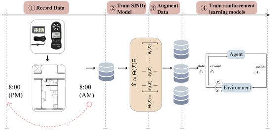
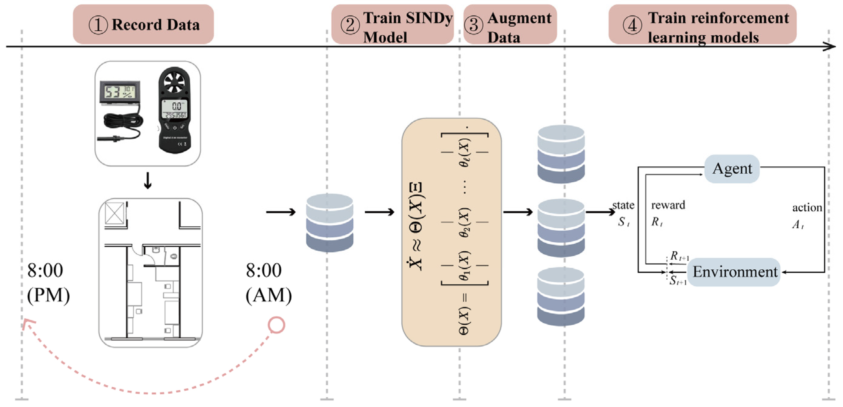
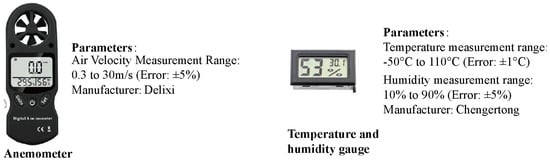
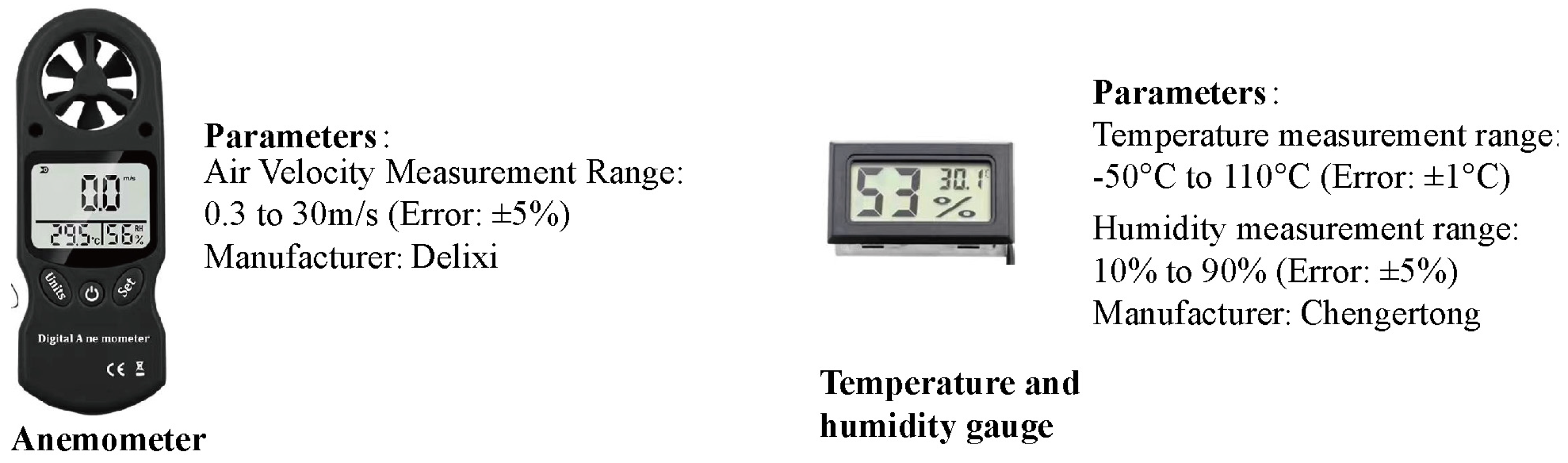
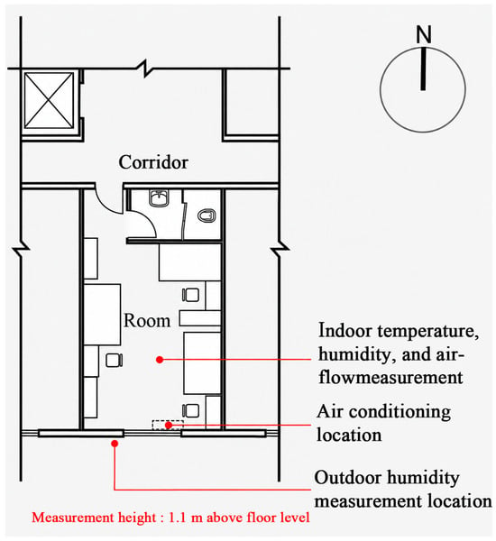
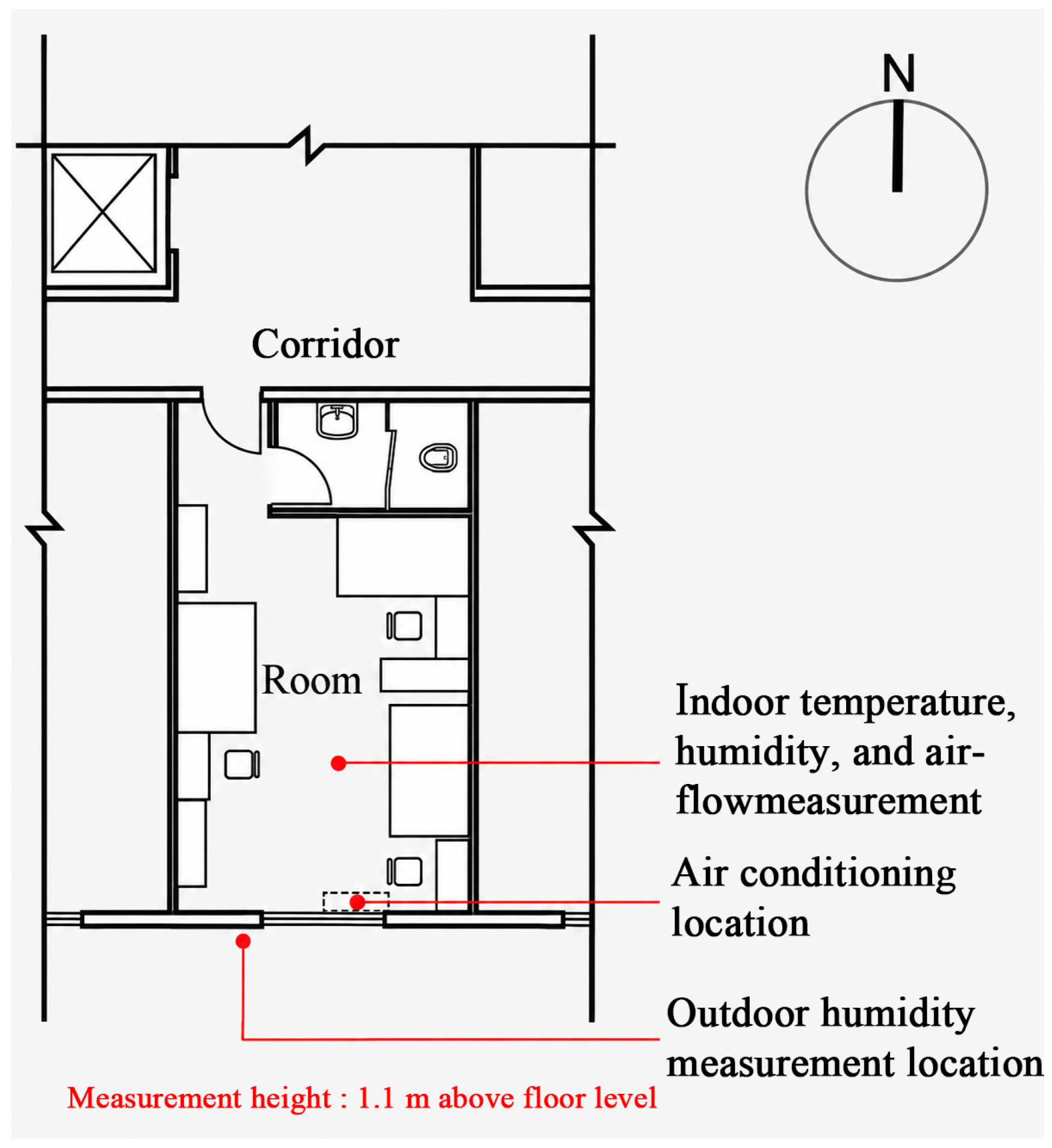
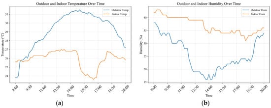
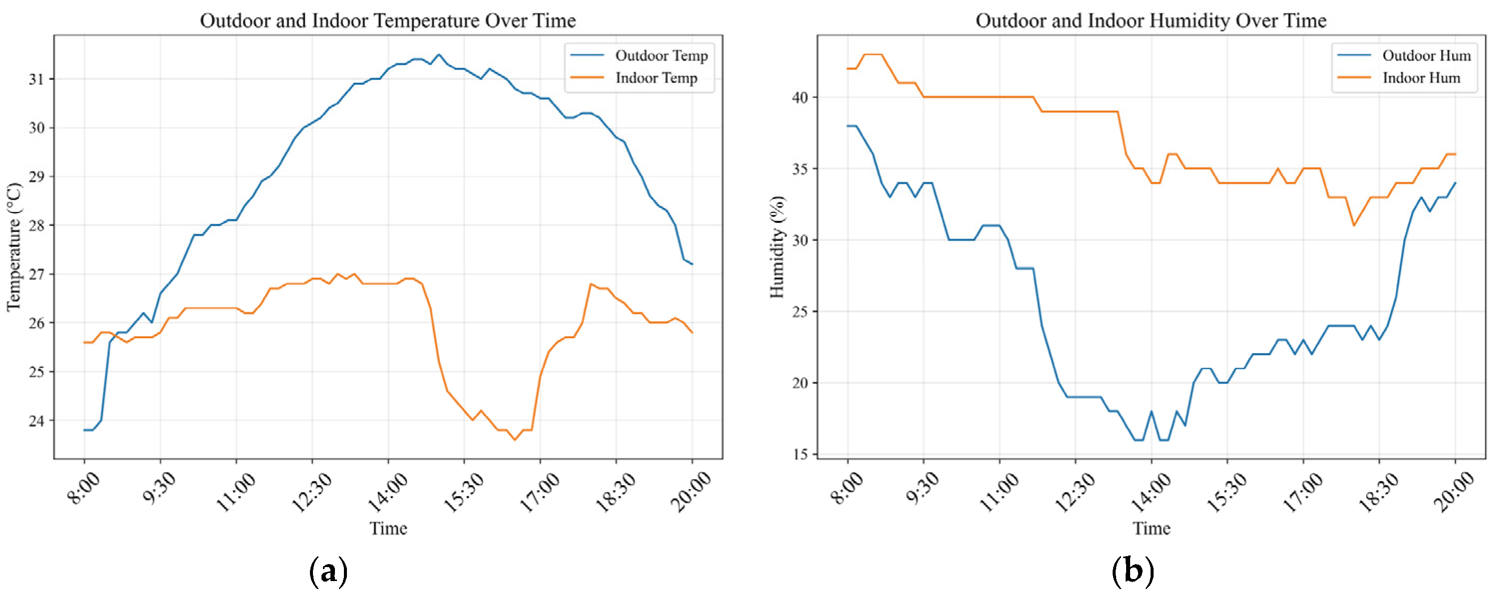
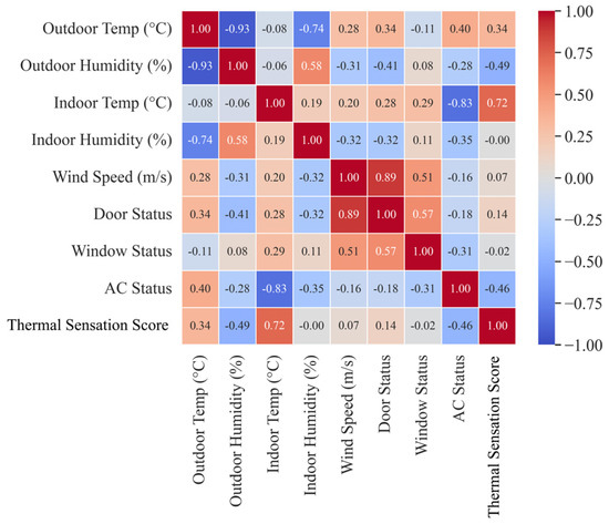
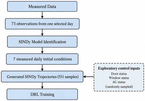
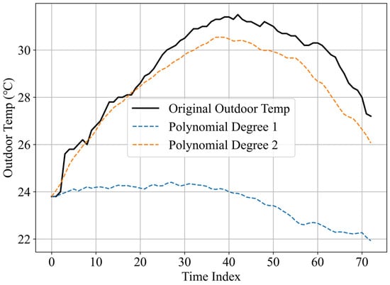
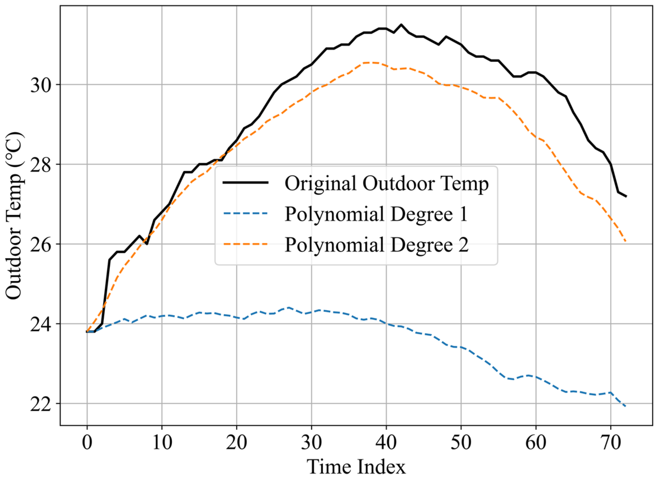
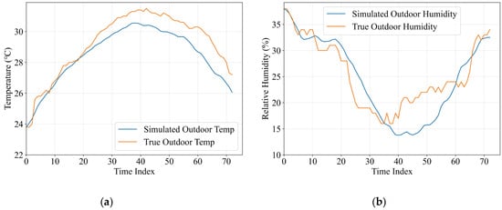
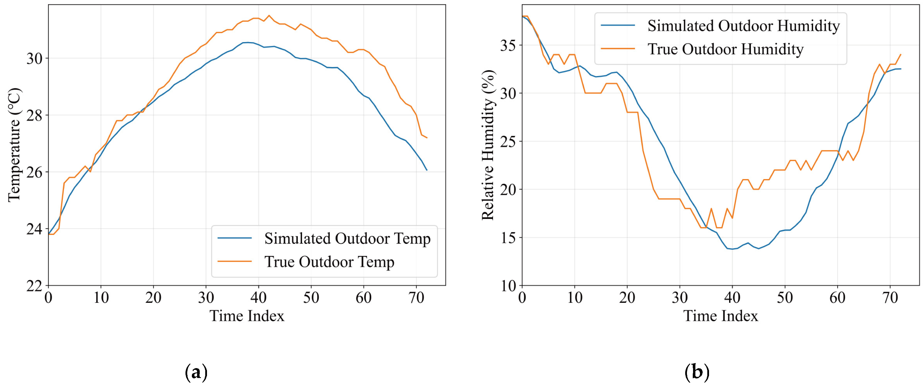
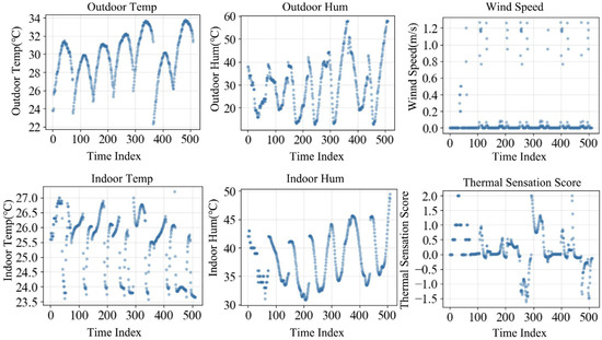
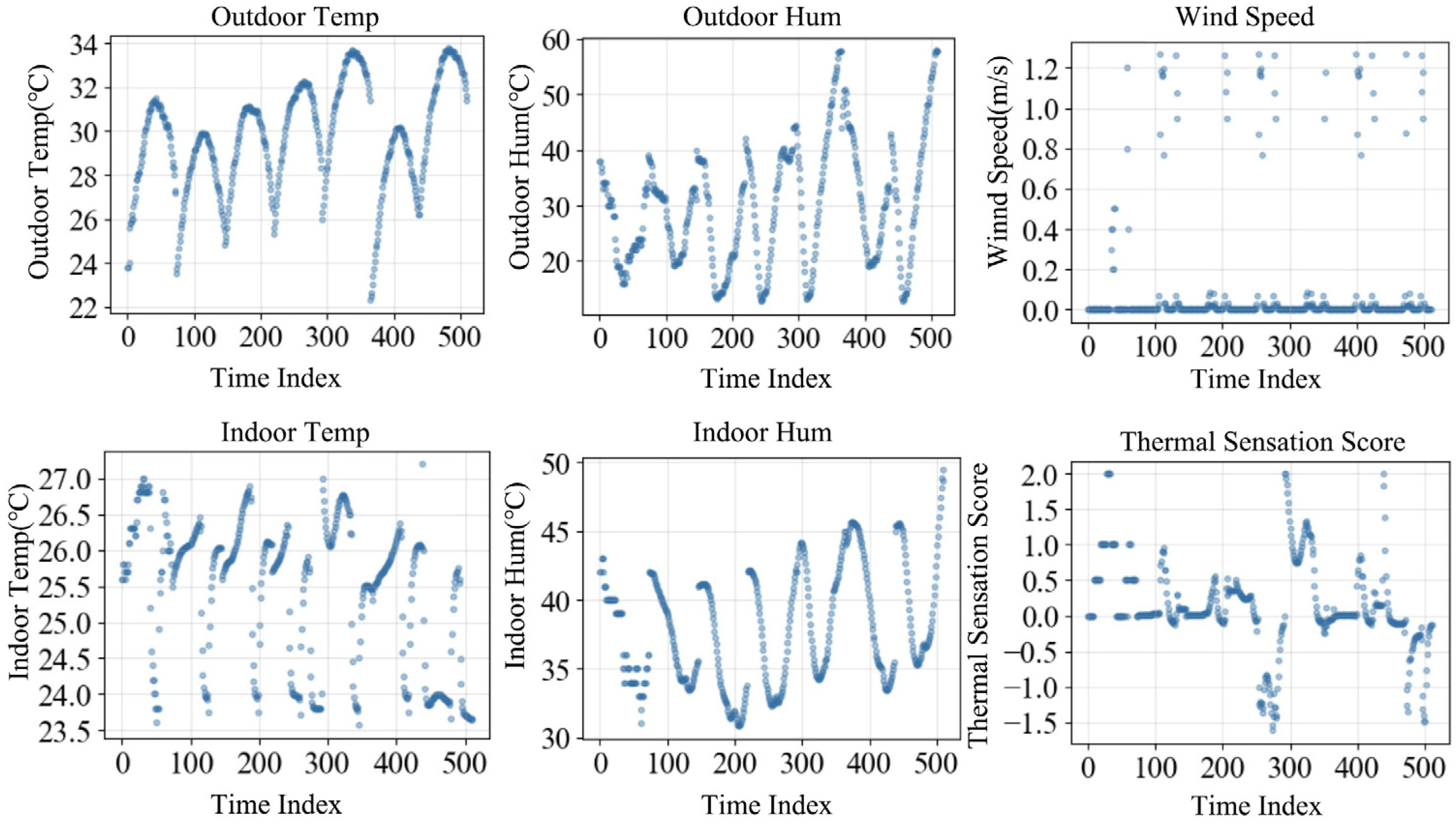
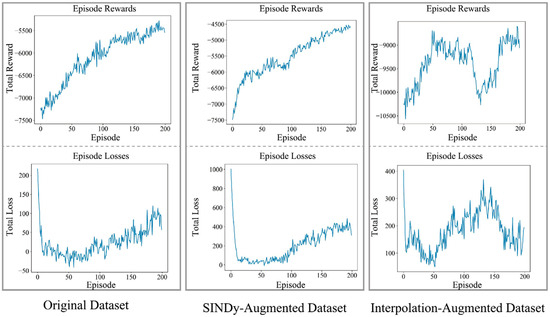
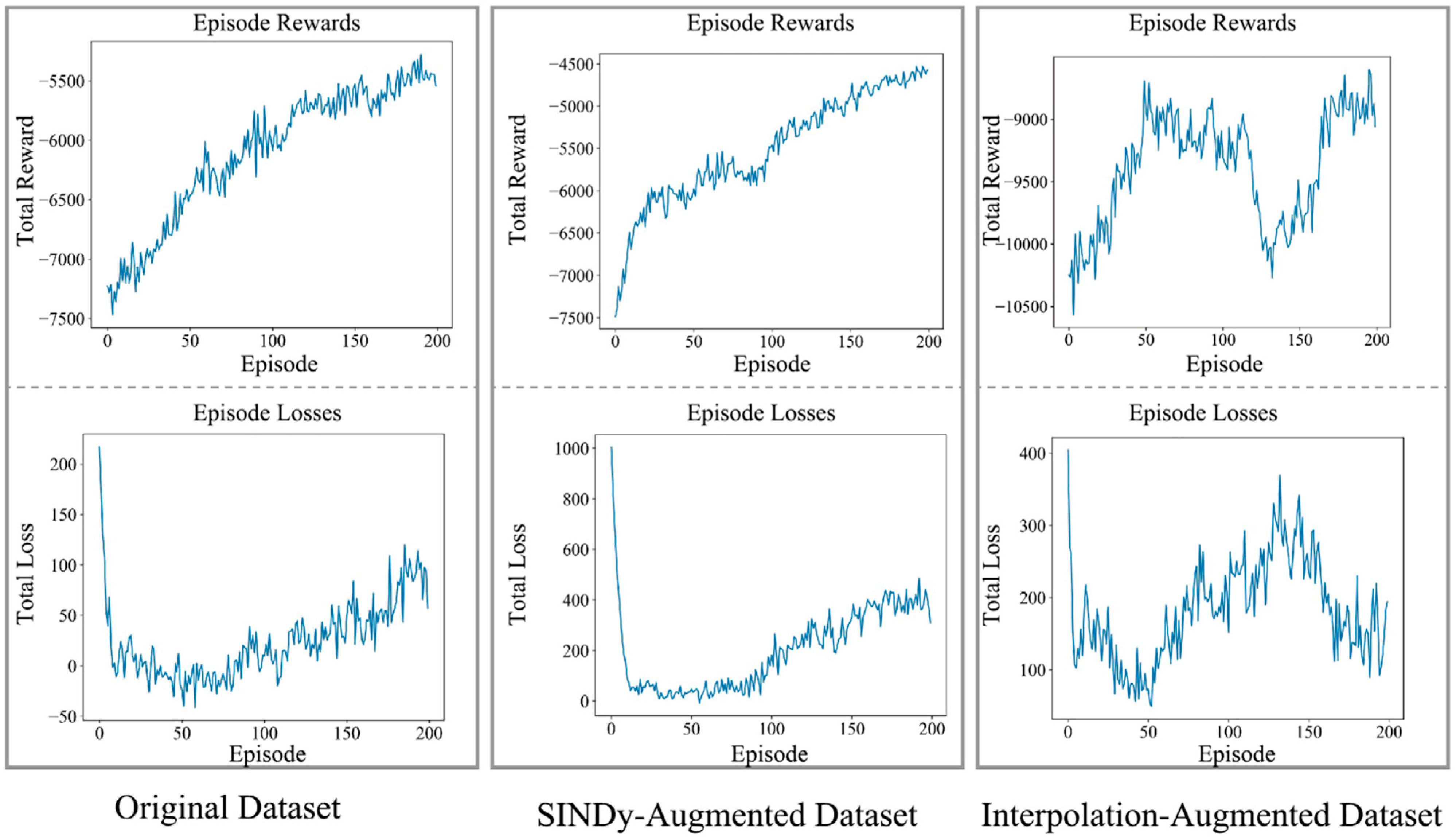

Disclaimer/Publisher’s Note: The statements, opinions and data contained in all publications are solely those of the individual author(s) and contributor(s) and not of MDPI and/or the editor(s). MDPI and/or the editor(s) disclaim responsibility for any injury to people or property resulting from any ideas, methods, instructions or products referred to in the content. |
© 2026 by the authors. Licensee MDPI, Basel, Switzerland. This article is an open access article distributed under the terms and conditions of the Creative Commons Attribution (CC BY) license.