Risk Assessment of Shield Tunnelling in Mixed Ground Using a Coupled Subjective–Objective Weighting and Fuzzy Set Pair Analysis Model

Abstract

Shield tunnelling in upper-soft and lower-hard mixed ground is characterised by strong geological heterogeneity and coupled construction risks, including uneven cutterhead loading, face instability, cutter wear and abnormal fluctuations in tunnelling parameters. This study assessed risk of shield tunnelling under such conditions by using a coupled subjective–objective weighting and fuzzy set pair analysis model. Seven key tunnelling parameters, namely total thrust, advance rate, cutterhead rotational speed, cutterhead torque, chamber pressure, grouting pressure and shield attitude, are selected as evaluation indicators. The Analytic Hierarchy Process (AHP) and coefficient of variation method are combined to determine indicator weights, thereby integrating expert judgement with the statistical characteristics of field data. A five-element connection number is then introduced to characterise the identity–discrepancy–contrary relationships between measured indicator values and risk grade standards, while segmented triangular fuzzy numbers are used to determine discrepancy coefficients and address the fuzziness of grade boundaries. The results show that the risk grades for Rings 1–500 fluctuate considerably and are dominated by Grade II–III risks, with 11% of the evaluated segments reaching Grade IV. For Rings 501–1000, the predicted risk level is generally lower, with Grade II and Grade III accounting for 29% and 67% of the evaluated segments, respectively. The assessment results are consistent with the geological conditions and construction observations, indicating that the model can effectively quantify shield tunnelling risk and identify key high-risk parameters in mixed ground. The proposed hybrid framework provides a new theoretical reference for real-time dynamic risk assessment of shield tunnelling under geological transitional conditions.

1. Introduction

Shield tunnelling is widely used in mechanised underground construction because it can provide efficient excavation with relatively limited disturbance to the surrounding environment [1,2,3,4,5]. However, tunnelling performance and construction safety depend strongly on the interaction among the shield machine, the ground conditions and the operating regime. This interaction becomes particularly complex in upper-soft/lower-hard mixed ground, where the excavation face intersects materials with substantially different stiffness, strength, permeability and weathering characteristics. Such geological heterogeneity may lead to uneven cutterhead loading, fluctuating thrust and torque, excessive cutter wear, face instability, ground deformation and difficulties in maintaining stable shield operation [6,7,8,9]. Therefore, risk assessment in mixed ground should consider both the spatial variability of the geological environment and the temporal variation in operational parameters. In addition, face-support and grouting conditions require careful interpretation, because low chamber or grouting pressure cannot automatically be regarded as safe without considering the ground and groundwater conditions [10].

Risk assessment provides a systematic framework for identifying, analysing and managing these uncertainties. Early studies established the basis for risk analysis in underground engineering. Einstein [11] discussed the application of risk analysis in rock engineering, while Sturk et al. [12] incorporated probabilistic analysis and decision theory into the assessment of large underground projects. Reilly [13] emphasised the importance of lifecycle risk management for complex tunnelling projects, and the International Tunnelling and Underground Space Association provided guidelines for risk identification, analysis and treatment [14]. Building on these foundations, various quantitative approaches have been applied to tunnel construction, including Bayesian networks for updating conditional risks [15], fault-tree and event-tree methods for analysing accident pathways [16,17], the Analytic Hierarchy Process (AHP) for determining the relative importance of risk indicators [18], fuzzy-set methods for representing imprecise expert knowledge [19,20], cloud models for describing fuzziness and randomness [21], and fuzzy AHP for ranking geological risks in mechanised tunnelling [22]. These methods are complementary rather than interchangeable, because they require different types of information and produce different forms of risk output.

Recent research has increasingly combined shield-operational data with geological and ground-response information. Jiang et al. [23] investigated an in situ monitoring system for ground displacement induced by shield tunnelling. Yan [24] documented ring-level geological and operational data from EPB shield tunnelling in mixed soil and rock ground, demonstrating the value of linking geological classifications with machine records. Guo et al. [25] analysed the relationship between construction parameters and ground settlement under soil–rock mixed-face conditions. These studies indicate that operational parameters can provide useful information about changing ground conditions. However, operational measurements should be interpreted together with independent geological, deformation or construction-response data.

Data-driven prediction and early-warning methods have also developed rapidly. Loy-Benitez et al. [26] proposed a convolutional variational-autoencoder framework for monitoring sinkhole-related anomalies during EPB shield tunnelling in mixed-face ground. Deng et al. [27] combined multivariate data fusion with catastrophe theory to forecast and provide early warning of shield-tunnelling-induced ground collapse at a rock-soil interface. Hu and Cheng [28] developed an Informer-based framework for long-distance shield-performance prediction using operational, monitoring and stratigraphic information. These studies address different assessment objectives, including geological classification, performance prediction, ground-settlement forecasting and event warning. Their performance measures therefore cannot be directly compared with the proportion of tunnel segments assigned to a particular risk grade.

Recent risk-assessment studies have also moved beyond single-method frameworks. Chung et al. [29] proposed a causal-network-based risk matrix for shield TBM projects. Other studies have applied variable-weight theory with cloud models [30], hybrid cloud-model and Bayesian-network methods [31], settlement-risk models for slurry-balance shield tunnelling [32] and improved nonlinear fuzzy AHP [33]. Sun et al. [34] further combined G1 and entropy weights through game theory and incorporated variable weights and an extension cloud model into the assessment of metro shield-tunnelling risk. These studies demonstrate that subjective–objective weighting and hybrid uncertainty models are already active areas of research.

Despite this progress, a practical need remains for an interpretable procedure that can convert multiple operational observations into segment-level risk information under mixed-ground conditions. Bayesian, event-tree and machine-learning methods are valuable for causal analysis, event forecasting and anomaly detection, but they may require probabilistic assumptions, predefined causal structures or large labelled datasets. Cloud, extension and grey-system methods provide alternative representations of uncertainty, although their outputs and parameter meanings may be less directly connected to the identity or deviation of individual tunnelling indicators. Set Pair Analysis (SPA) is therefore adopted in this study because it can explicitly represent the identity–discrepancy–contrary relationship between measured values and risk standards and describe gradual transitions between adjacent risk grades.

This study develops a coupled subjective–objective weighting and fuzzy set pair analysis framework for shield tunnelling in upper-soft/lower-hard mixed ground. The AHP and coefficient-of-variation (CV) methods are used to represent expert-assessed importance and data variability, respectively. SPA is then used to describe the identity–discrepancy–contrary relationship between measured operational values and project-specific grading standards. The proposed framework is applied to the Hualong Station–Mingjingcun Shaft section of the Pearl River Delta Intercity Railway Pazhou Branch in Guangzhou, Guangdong Province, China. Seven operational indicators are considered (i.e., total thrust, advance rate, cutter-head rotational speed, cutter-head torque, chamber pressure, grouting pressure and shield attitude). Measured operational data are used for Rings 1–500, whereas the supplied case dataset describes Rings 501–1000 using predicted inputs. The data are grouped into five-ring segments to obtain segment-level assessments.

2. Materials and Methods

2.1. Project Overview and Field Monitoring Dataset

The project was located in the Hualong Station–Mingjingcun Shaft section of the Pazhou Branch of the Pearl River Delta Intercity Railway in Guangzhou, Guangdong Province, China. The left-line tunnel has a total length of approximately 2.535 km and was constructed using an earth-pressure-balance (EPB) shield machine. The tunnel lining has an outer diameter of 8.8 m, an inner diameter of 8.0 m and a ring width of 1.8 m. The shield cutterhead has an excavation diameter of 9140 mm.

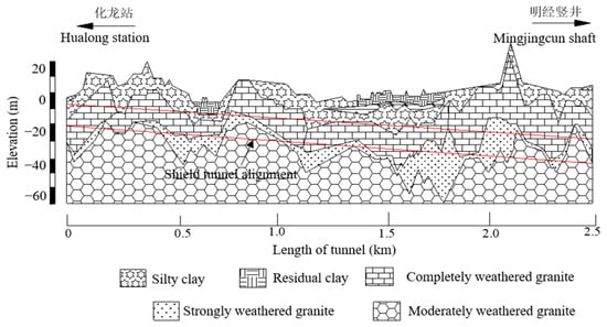
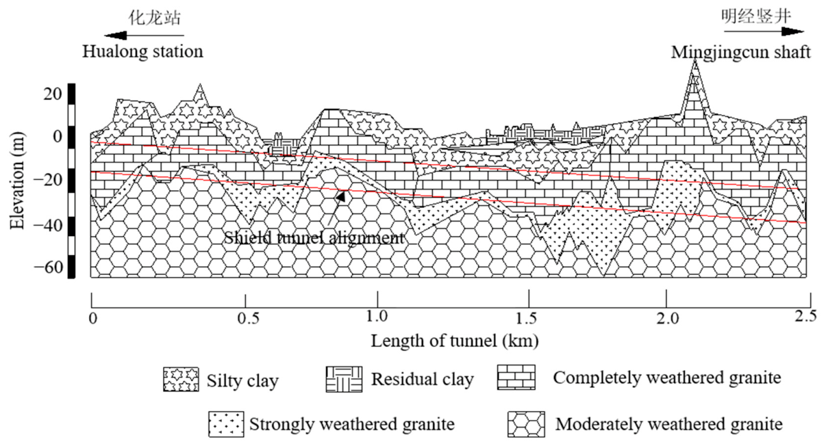
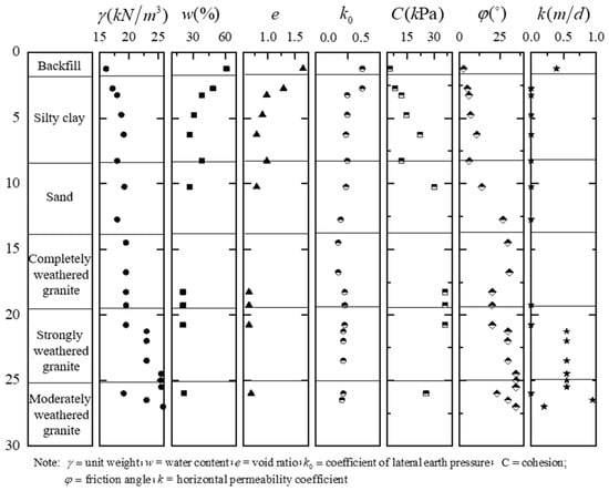
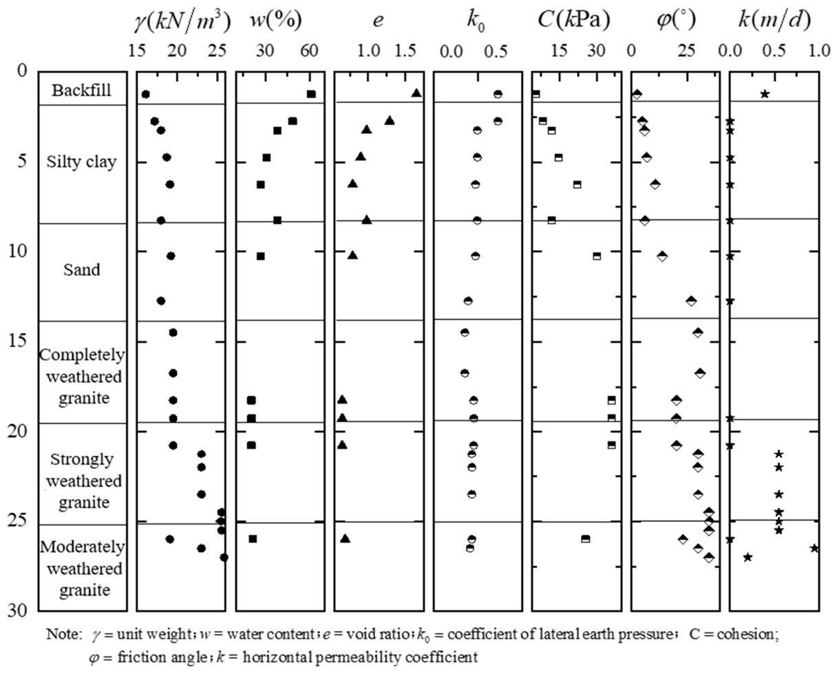
The geological profile and the distribution of the main strata are shown in Figure 1, while the relevant physical and mechanical properties are presented in Figure 2. The tunnel alignment passes mainly through granite formations with different weathering degrees. Completely weathered granite and strongly weathered granite occur along considerable portions of the alignment, while moderately weathered granite locally appears in the lower part of the excavation face. Silty clay and sand layers are also present in some sections, particularly near the upper part of the tunnel face. Consequently, the shield frequently encounters upper-soft/lower-hard or mixed-face ground conditions, in which soil and rock with substantially different stiffness, strength, permeability and abrasivity are excavated simultaneously.

Figure 1. Geological profile along the tunnel.

Figure 2. Parameters of soils and rocks.

The dataset in this study consists of the set of actual shield tunnelling parameter values and the set of evaluation standard indicator values. The actual values comprise the measured values from Rings 1–500 and the predicted values from Rings 501–1000, as shown in Table 1. The measured values of indicator parameters for Rings 1–500 were compiled during the construction process, while the predicted values for Rings 501–1000 were obtained using machine learning methods. The statistical characteristics of the actual indicator values are presented in Table 2. It is worth noting that the tunnelling parameter of shield attitude includes two sub-indicators of horizontal deviation and vertical deviation. For construction, a larger deviation implies higher risk. Therefore, when constructing the shield attitude set, the larger absolute value of the horizontal deviation and vertical deviation is directly used for subsequent analysis and calculation.

Table 1. Statistics of parameter values for each indicator.

Ring No.		Measured							Predicted
		R1	⋯	R496	R497	R498	R499	R500	R501	…	R1000
Total thrust (A1)		13,000	…	26,000	25,000	25,000	25,000	25,000	28,000	…	26,606
Advance rate (A2)		16	…	30	40	26	24	26	39.513	…	40.763
Cutterhead rotational speed (A3)		1.2	…	2.0	2.0	2.0	2.0	2.0	2.0	…	1.880
Cutterhead torque (A4)		3200	…	5300	5200	5200	5100	5100	5300	…	4967
Chamber pressure (A5)		10	…	210	210	210	210	210	210	…	193
Grouting pressure (A6)		180	…	360	290	290	290	290	320	…	291
Attitude (A7)	Horizontal trend	0.400	…	−0.067	0.933	0.667	0.333	0	−1.333	…	−0.111
	Vertical trend	5.574	…	−1.311	−2.186	0.437	0.546	0.656	0.984	…	−0.283

Table 2. Statistical characteristics of actual indicator values.

Indicator		Left Line Rings 1–500			Left Line Rings 501–1000
		Maximum	Minimum	Average	Maximum	Minimum	Average
Total thrust (A1)		39,000	3700	26,307	40,000	18,000	25,860
Advance rate (A2)		80	1.6	35.697	50	10	39.245
Cutterhead rotational speed (A3)		2	1	1.72	2.1	1.2	1.749
Cutterhead torque (A4)		6900	2100	4343.762	8000	2100	4428.27
Chamber pressure (A5)		220	0	147.430	210	0	180.434
Grouting pressure (A6)		370	100	293.46	330	170	311.838
Shield attitude (A7)	Horizontal trend	4.800	−2.800	|0.445|	1.267	−2.400	|0.255|
	Vertical trend	9.508	−6.885	|1.038|	10.737	−4.044	|0.808|

2.2. Coupled Subjective–Objective Weighting and Fuzzy Set Pair Analysis Model

This section establishes the core methodological framework of the paper, addressing four components in sequence. First, the combined subjective–objective weighting model integrating the AHP and the coefficient of variation method is introduced to resolve the issues of subjective bias and statistical blind spots inherent in single-method weighting approaches. Second, the fundamental theory of set pair analysis (SPA) is presented, where the identity–discrepancy–contrary connection number is employed to characterise both certainty and uncertainty in a unified manner. Third, the principle of triangular fuzzy numbers is explained, providing a mathematical tool for handling the fuzziness at grade boundaries. Finally, SPA and triangular fuzzy numbers are coupled into an integrated mathematical framework for risk assessment.

2.2.1. Combined Subjective–Objective Weighting Method

The rational allocation of indicator weights is a prerequisite for risk assessment. Weight determination methods can be categorised into subjective and objective approaches. Subjective weighting methods (e.g., AHP) rely on expert experience and judgement, reflecting the engineering importance ranking of indicators, but are limited by a degree of subjective arbitrariness. Objective weighting methods (e.g., the coefficient of variation method) determine weights based solely on the degree of dispersion inherent in the data, free from human interference, yet may overlook the practical physical significance of the indicators. A single weighting method cannot adequately fulfil both requirements. Therefore, this study adopts a combined weighting strategy integrating AHP and the coefficient of variation method, optimising the fusion ratio of subjective and objective weights through the coefficient of difference method to achieve precise weight allocation.

AHP constructs a hierarchical structure model in which experts perform pairwise comparisons of indicators at the same level using a 1–9 ratio scale (as shown in Table 3) to determine their relative importance, thereby establishing a judgement matrix (as shown in Table 4). From the judgement matrix, the relative weight of each factor with respect to its criterion is calculated, enabling ranking of the factors. This ranking essentially involves computing the eigenvalues and eigenvectors of the judgement matrix. The maximum eigenvalue of the judgement matrix is first determined, and then the corresponding eigenvector can be solved according to Equation (1), where the components represent the factor weights.

AW₁ = λ_maxW₁

(1)

where A is the judgement matrix; λ_max is the maximum eigenvalue and W₁ is the corresponding eigenvector. Once the maximum eigenvalue is obtained, a consistency check must be performed on the judgement matrix as follows.

Table 3. Meanings of the ratio scales.

Scale Values	Meanings
1	Factor Ai is equally important as factor Aj
3	Factor Ai is slightly more important than factor Aj
5	Factor Ai is clearly more important than factor Aj
7	Factor Ai is very strongly more important than factor Aj
9	Factor Ai is extremely more important than factor Aj
2, 4, 6, 8	Intermediate values between two adjacent judgement levels

Table 4. Judgement matrix.

Criterion	A1	A2	⋯	An
A1	a11	a12	⋯	a1n
A2	1/a12	a22	⋯	a2n
⋯	⋯	⋯	⋯	⋯
An	1/a1n	1/a2n	⋯	ann

The consistency index (CI)is calculated using Equation (2).

$$\mathit{CI}={\displaystyle \frac{{\lambda }_{\max }-n}{n-1}}$$

(2)

where n is the number of evaluation indicators.

The average random consistency index (RI) can be obtained according to Table 5. The consistency ratio (CR) can be calculated using Equation (3). If CR is less than 0.1, the consistency of the judgement matrix is deemed acceptable; otherwise, the judgement matrix should be appropriately revised.

$$\mathit{CR}={\displaystyle \frac{\mathit{CI}}{\mathit{RI}}}$$

(3)

Table 5. RI values for low-order judgement matrices.

Order	1	2	3	4	5	6	7	8	9	10	11
RI	0.00	0.00	0.58	0.90	1.12	1.24	1.32	1.41	1.45	1.49	1.52

The coefficient of variation method determines objective weights based on the degree of variability in the measured data of each indicator, effectively eliminating the influence of dimensional differences on weight calculation. The core principle is that the larger the coefficient of variation in an indicator’s data, the stronger its discriminative power among different evaluation samples is, and thus the higher the weight it should be assigned.

The calculation procedure involves first computing the ratio of the standard deviation (σ_i, i = 1, 2, …, n) to the mean (${\overline{x}}_i$) for each indicator to obtain the coefficient of variation (cv_i) using Equation (4), and then normalising the coefficients of variation in all indicators to obtain the objective weight (ω_i) using Equation (5).

$$c{v}_i={\displaystyle \frac{{\sigma }_i}{{\overline{x}}_i}}$$

(4)

$${\omega }_i={\displaystyle \frac{c{v}_i}{{\displaystyle \sum _{i=1}^{n}c{v}_i}}}$$

(5)

The final objective weight vector can be obtained as W₂ = {ω₁,ω₂,⋯,ω_n}.

In practical applications, linear weighted combination is commonly adopted, as it overcomes the weight multiplication effect that arises from multiplication-based synthesis and normalisation methods. Therefore, this study employs linear weighting to combine the subjective and objective weights. The combined weight vector (W) is given as follows.

W = αW₁ + (1 − α)W₂

(6)

where α is the combination coefficient representing the proportion of the subjective and objective weights in the combined weight. In this study, α is determined using the coefficient of difference method, calculated as follows.

$$\alpha ={\displaystyle \frac{n}{n-1}}\left[{\displaystyle \frac{2}{n}}\left({\omega }_{1,1}+2{\omega }_{1,2}+\cdots +n{\omega }_{1,n}\right)-{\displaystyle \frac{n+1}{n}}\right]$$

(7)

where ω_1,i (i = 1, 2, …, n) is the ascending-order sorted subjective weights.

2.2.2. Basic Theory of Set Pair Analysis

While the combined weighting method described above addresses the quantification of the relative importance of indicators, another core challenge in risk assessment remains how to accurately characterise the fuzzy transitional relationship between measured indicator values and risk grade standards. The rigid truncation of membership functions in conventional fuzzy comprehensive evaluation often leads to misjudgement at grade boundaries. SPA is an effective method for handling uncertain systems from the three dimensions of identity, discrepancy, and contrary. Two interrelated sets A and B form a set pair H = (A, B). The identity–discrepancy–contrary relationship between them is described by a connection number μ(A,B), whose basic form is as follows.

$$\mu \left(A,B\right)={\displaystyle \frac{S}{N}}+{\displaystyle \frac{F}{N}}i+{\displaystyle \frac{P}{N}}j=a+\mathit{bi}+\mathit{cj}$$

(8)

N = S + F + P

(9)

$$a={\displaystyle \frac{S}{N}},\hspace{1em}b={\displaystyle \frac{F}{N}},\hspace{1em}c={\displaystyle \frac{P}{N}}$$

(10)

where S denotes the number of identical characteristics between sets A and B; F denotes the number of discrepant characteristics between sets A and B; P denotes the number of contrary characteristics between sets A and B; N denotes the total number of characteristics or evaluation indicators; a, b and c represent the degree of identity, degree of discrepancy and degree of contrary of the set pair, respectively, satisfying a + b + c = 1; i is the discrepancy coefficient, taking values in [−1, 1]; j is the contrary coefficient, typically taken as −1.

For five-grade risk assessment, the discrepancy term is expanded into three components, and a five-element connection number is employed to accurately characterise the gradual risk transition process.

μ = a + b₁i₁ + b₂i₂ + b₃i₃ + cj

(11)

where a + b₁ + b₂ + b₃ + c = 1, and a, b₁, b₂, b₃, c in [0, 1]; b₁, b₂, and b₃ are the discrepancy components; and i₁, i₂, and i₃ are the corresponding discrepancy coefficients.

2.2.3. Principle of Triangular Fuzzy Numbers

The discrepancy coefficients i₁, i₂, and i₃ in set pair analysis must take specific values within the interval [−1, 1], and the precision of these values directly affects the accuracy of the risk assessment results. Triangular fuzzy numbers, with their simple membership function form and favourable computational properties, provide an effective mathematical tool for the continuous solution of discrepancy coefficients. This section introduces the basic definition of triangular fuzzy numbers.

Let $\tilde{\mathrm{A}}$ be a fuzzy number defined on the real domain R, with its membership function ${\mu }_{\tilde{\mathrm{A}}}\left(x\right)$ given by,

$${\mu }_{\tilde{\mathrm{A}}}\left(x\right):R\to \left[0,1\right](x\in R)$$

(12)

where x is the value of the indicator.

If the membership function is expressed as,

$${\mu }_{\tilde{\mathrm{A}}}\left(x\right)=\left\{\begin{array}{l}0\hspace{1em}\hspace{1em}\hspace{1em}x\le x_1\\ {\displaystyle \frac{x-x_1}{x_2-x_1}}\hspace{1em}{x}_1<x\le x_2\\ {\displaystyle \frac{x_3-x}{x_3-x_2}}\hspace{1em}{x}_2<x\le x_3\\ 0\hspace{1em}\hspace{1em}\hspace{1em}x>x_3\end{array}\right.$$

(13)

then $\tilde{\mathrm{A}}$ is called a triangular fuzzy number, denoted as $\tilde{\mathrm{A}}=\left(x_1,x_2,x_3\right)$. Here x₁,x₂,x₃ are real numbers and x₁ ≤ x₂ ≤ x₃. When x₁ = x₂ = x₃, $\tilde{\mathrm{A}}$ is an exact number. In practical applications, a segmented triangular fuzzy number is often employed, whose membership function can be expressed as,

$${\mu }_{\tilde{\mathrm{A}}}\left(x\right)=\left\{\begin{array}{l}0\hspace{1em}\hspace{1em}\hspace{1em}\hspace{1em}\hspace{1em}\hspace{1em}x\le x_1\\ x-x_1/x_2-x_1\hspace{1em}{x}_1<x\le x_2\\ x_3-x/x_3-x_2\hspace{1em}{x}_2<x\le x_3\\ 0\hspace{1em}\hspace{1em}\hspace{1em}\hspace{1em}\hspace{1em}\hspace{1em}{x}_3<x\le x_4\\ x-x_4/x_5-x_4\hspace{1em}{x}_4<x\le x_5\\ x_6-x/x_6-x_5\hspace{1em}{x}_5<x\le x_6\\ 0\hspace{1em}\hspace{1em}\hspace{1em}\hspace{1em}\hspace{1em}\hspace{1em}x>x_6\end{array}\right.$$

(14)

In this case, $\tilde{\mathrm{A}}$ is called a segmented triangular fuzzy number, denoted as $\tilde{\mathrm{A}}=\left(x_1,x_2,x_3,x_4,x_5,x_6\right)$, where x₁ ≤ x₂ ≤ x₃ ≤ x₄ ≤ x₅ ≤ x₆. It is noteworthy that the range of the membership function is [0, 1].

2.2.4. Construction of the Coupled Model

The integration of set pair analysis with triangular fuzzy numbers primarily involves applying triangular fuzzy numbers to perform uncertainty analysis on the discrepancy coefficients in the multi-element connection number expression. For a practical uncertainty evaluation problem with five classification grades, a five-element connection number can be used to reflect the identity–discrepancy–contrary system structure.

Let the evaluation indicator be n(n = 1,2,⋯,N), and the upper boundary values of the evaluation grades be S_n,k(k = 1,2,⋯,4). When the indicator value of a sample is less than the Grade I standard boundary (denoted as S_n,1), the indicator value and the standard value are defined as being in an identity relationship, and the corresponding identity coefficient is taken as 1. When the indicator value of the sample to be evaluated exceeds the Grade IV standard boundary (S_n,4), it is defined as being in a contrary relationship, and the contrary coefficient (j) is taken as −1. For sample values falling within the Grade II, III, and IV standard boundary ranges, they are defined as discrepancy; these sample values require further refinement. Sample values conforming to Grade II, III, and IV standards are defined as partial-identity discrepancy, intermediate discrepancy, and partial-contrary discrepancy, respectively. Correspondingly, i₁, i₂, and i₃ represent the partial-identity discrepancy coefficient, intermediate discrepancy coefficient, and partial-contrary discrepancy coefficient, respectively. The corresponding connection number expression is as follows.

$${\mu }_{\mathit{pn}}=\left\{\begin{array}{l}1+0i_1+0i_2+0i_3+0j\hspace{1em}\hspace{1em}\hspace{1em}\hspace{1em}\hspace{1em}\hspace{1em}\hspace{1em}\hspace{1em}\hspace{1em}\hspace{1em}\hspace{1em}\hspace{1em}\hspace{1em}\hspace{1em}{s}_{\mathit{pn}}\le s_{n,1}\\ {\displaystyle \frac{2s_{\mathit{pn}}-s_{n,1}-s_{n,2}}{s_{n,1}-s_{n,2}}}+{\displaystyle \frac{2s_{n,1}-2s_{\mathit{pn}}}{s_{n,1}-s_{n,2}}}{i}_1+0i_2+0i_3+0j\hspace{1em}\hspace{1em}\hspace{1em}\hspace{1em}{s}_{n,1}<s_{\mathit{pn}}\le {\displaystyle \frac{s_{n,1}+s_{n,2}}{2}}\\ 0+{\displaystyle \frac{2s_{\mathit{pn}}-s_{n,2}-s_{n,3}}{s_{n,1}-s_{n3}}}{i}_1+{\displaystyle \frac{s_{n,1}+s_{n,2}-2s_{\mathit{pn}}}{s_{n,1}-s_{n3}}}{i}_2+0i_3+0j\hspace{1em}\hspace{1em}{\displaystyle \frac{s_{n,1}+s_{n,2}}{2}}<s_{\mathit{pn}}\le {\displaystyle \frac{s_{n,2}+s_{n,3}}{2}}\\ 0+0i_1+{\displaystyle \frac{2s_{\mathit{pn}}-s_{n,3}-s_{n,4}}{s_{n,2}-s_{n,4}}}{i}_2+{\displaystyle \frac{s_{n,2}+s_{n,3}-2s_{\mathit{pn}}}{s_{n,2}-s_{n,4}}}{i}_3+0j\hspace{1em}\hspace{1em}{\displaystyle \frac{s_{n,2}+s_{n,3}}{2}}<s_{\mathit{pn}}\le {\displaystyle \frac{s_{n,3}+s_{n,4}}{2}}\\ 0+0i_1+0i_2+{\displaystyle \frac{2s_{\mathit{pn}}-2s_{n,4}}{s_{n,3}-s_{n,4}}}{i}_3+{\displaystyle \frac{s_{n,3}+s_{n,4}-2s_{\mathit{pn}}}{s_{n,3}-s_{n,4}}}j\hspace{1em}\hspace{1em}\hspace{1em}\hspace{1em}{\displaystyle \frac{s_{n,3}+s_{n,4}}{2}}<s_{\mathit{pn}}\le s_{n,4}\\ 0+0i_1+0i_2+0i_3+1j\hspace{1em}\hspace{1em}\hspace{1em}\hspace{1em}\hspace{1em}\hspace{1em}\hspace{1em}\hspace{1em}\hspace{1em}\hspace{1em}\hspace{1em}\hspace{1em}\hspace{1em}\hspace{1em}{s}_{\mathit{pn}}>s_{n,4}\end{array}\right.$$

(15)

where μ_pn is the connection number of the n-th indicator of the sample p, and s_pn is the value of the sample evaluation indicator.

The determination of the discrepancy coefficients in the multi-element connection number constitutes the most critical step in SPA. This study introduces segmented triangular fuzzy numbers to solve for these coefficients. The discrepancy coefficient values corresponding to other indicator values can be solved according to the principle of triangular fuzzy numbers as follows.

$$i_1=\left\{\begin{array}{l}{\displaystyle \frac{s_{n,1}-s_{\mathit{pn}}}{s_{n,1}-s_{n,2}}}\hspace{1em}\hspace{1em}\hspace{1em}\hspace{1em}\hspace{1em}\hspace{1em}\hspace{1em}{s}_{n,1}<s_{\mathit{pn}}\le {\displaystyle \frac{s_{n,1}+s_{n,2}}{2}}\\ {\displaystyle \frac{2s_{\mathit{pn}}-s_{n,2}-s_{n,3}}{2\left(s_{n,1}-s_{n,3}\right)}}\hspace{1em}\hspace{1em}\hspace{1em}\hspace{1em}{\displaystyle \frac{s_{n,1}+s_{n,2}}{2}}<s_{\mathit{pn}}\le {\displaystyle \frac{s_{n,2}+s_{n,3}}{2}}\\ 0\hspace{1em}\hspace{1em}\hspace{1em}\hspace{1em}\hspace{1em}\hspace{1em}\hspace{1em}\hspace{1em}\hspace{1em}\hspace{1em}\mathrm{others}\end{array}\right.$$

(16)

$$i_2=\left\{\begin{array}{l}{\displaystyle \frac{2s_{\mathit{pn}}-s_{n,1}-s_{n,2}}{2\left(s_{n,3}-s_{n,1}\right)}}\hspace{1em}\hspace{1em}\hspace{1em}\hspace{1em}{\displaystyle \frac{s_{n,1}+s_{n,2}}{2}}<s_{\mathit{pn}}\le {\displaystyle \frac{s_{n,2}+s_{n,3}}{2}}\\ {\displaystyle \frac{2s_{\mathit{pn}}-s_{n,3}-s_{n,4}}{2\left(s_{n,2}-s_{n,4}\right)}}\hspace{1em}\hspace{1em}\hspace{1em}\hspace{1em}{\displaystyle \frac{s_{n,2}+s_{n,3}}{2}}<s_{\mathit{pn}}\le {\displaystyle \frac{s_{n,3}+s_{n,4}}{2}}\\ 0\hspace{1em}\hspace{1em}\hspace{1em}\hspace{1em}\hspace{1em}\hspace{1em}\hspace{1em}\hspace{1em}\hspace{1em}\hspace{1em}\mathrm{others}\end{array}\right.$$

(17)

$$i_3=\left\{\begin{array}{l}{\displaystyle \frac{2s_{\mathit{pn}}-s_{n,2}-s_{n,3}}{2\left(s_{n,2}-s_{n,4}\right)}}\hspace{1em}\hspace{1em}\hspace{1em}\hspace{1em}{\displaystyle \frac{s_{n,2}+s_{n,3}}{2}}<s_{\mathit{pn}}\le {\displaystyle \frac{s_{n,3}+s_{n,4}}{2}}\\ {\displaystyle \frac{s_{\mathit{pn}}-s_{n,4}}{s_{n,4}-s_{n,3}}}\hspace{1em}\hspace{1em}\hspace{1em}\hspace{1em}\hspace{1em}\hspace{1em}\hspace{1em}{\displaystyle \frac{s_{n,3}+s_{n,4}}{2}}<s_{\mathit{pn}}\le s_{n,4}\\ 0\hspace{1em}\hspace{1em}\hspace{1em}\hspace{1em}\hspace{1em}\hspace{1em}\hspace{1em}\hspace{1em}\hspace{1em}\hspace{1em}\mathrm{others}\end{array}\right.$$

(18)

2.3. Assessment Procedure for Shield Tunnel Construction Risk

2.3.1. Evaluation Indicators and Quantitative Classification

Based on the construction characteristics and main influencing factors of shield tunnelling, this study conducts risk assessment by adopting seven indicators, including total thrust (B₁), advance rate (B₂), cutterhead rotational speed (B₃), cutterhead torque (B₄), chamber pressure (B₅), grouting pressure (B₆) and shield attitude (B₇).

Drawing on engineering practice and experience from similar projects, each of the seven evaluation indicators is classified into five levels (as shown in Table 6), and the standard sets for the identity–discrepancy–contrary relationships of each indicator are established. The standard set corresponding to each indicator is as follows.

$$\begin{array}{l}{B}_1=\left\{\left[0,20,000\right),\left[20,000,40,000\right),\left[40,000,\infty \right)\right\}\\ B_2=\left\{\left[0,15\right),\left[15,60\right),\left[60,\infty \right)\right\}\\ B_3=\left\{\left[0,1.20\right),\left[1.20,1.75\right),\left[1.75,\infty \right)\right\}\\ B_4=\left\{\left[0,2000\right),\left[2000,7500\right),\left[7500,\infty \right)\right\}\\ B_5=\left\{\left[0,120\right),\left[120,200\right),\left[200,\infty \right)\right\}\\ B_6=\left\{\left[0,200\right),\left[200,350\right),\left[350,\infty \right)\right\}\\ B_7=\left\{\left[0,0.91\right),\left[0.91,5.45\right),\left[5.45,\infty \right)\right\}\end{array}$$

Table 6. Quantitative classification of evaluation indicators.

Indicator	Safe Grade I	Suitable Grade II	Slightly High Grade III	High Grade IV	Excessive Grade V
Total thrust (kN)	<20,000	20,000~30,000	30,000~35,000	35,000~40,000	>40,000
Advance rate (mm/min)	<15	15~30	30~45	45~60	>60
Cutterhead rotational speed (rpm)	<1.20	1.20~1.45	1.45~1.60	1.60~1.75	>1.75
Cutterhead torque (kN·m)	<2000	2000~3500	3500~5500	5500~7500	>7500
Chamber pressure (kPa)	<120	120~150	150~175	175~200	>200
Grouting pressure (kPa)	<200	200~250	250~300	300~350	>350
Shield attitude (mm/m)	<0.91	0.91~2.73	2.73~4.54	4.54~5.45	>5.45
	>−0.91	−0.91~−2.73	−2.73~−4.54	−4.54~−5.45	<−5.45

Taking the total thrust standard set B₁ as an example, when the measured value falls within the interval [0, 20,000), it is classified as identity. When it falls within [40,000, ∞), it is classified as contrary; and when it falls within [20,000, 40,000), it is classified as discrepancy, requiring further analysis.

2.3.2. Risk Level Evaluation Criteria

This study classifies shield tunnel construction risk into five levels, including Safe (I), Relatively Safe (II), Low Risk (III), Moderately High Risk (IV) and High Risk (V). The safety status descriptions corresponding to each level are presented in Table 7. The determination of the shield tunnel construction risk level in this study primarily considers the relationship between the actual values and standard values of the seven shield tunnelling indicators.

Table 7. Risk grades and safety status descriptions.

Grade	Risk	Safety Status Description
I	Safe	The indicator parameters comply with the corresponding standard values during shield tunnelling, and tunnel construction proceeds safely.
II	Relatively Safe	The indicator parameters are close to the corresponding standard values during shield tunnelling, and tunnel construction proceeds normally.
III	Low Risk	The indicator parameters deviate from the corresponding standard values, and tunnel construction faces a certain degree of risk.
IV	Moderately High Risk	The indicator parameters approach the boundary values, and tunnel construction faces considerable risk.
V	High Risk	The indicator parameters substantially exceed the boundary values, and tunnel construction faces extremely high risk.

When evaluating a practical problem, the connection number (μ_pn) of the n-th indicator of the sample is first calculated. The weights of each indicator (ω_n) are then determined. The comprehensive connection number (μ_p) is calculated using the following equation.

$${\mu }_p={\displaystyle \sum _{n=1}^N{w}_n{\mu }_{\mathit{pn}}}$$

(19)

The maximum membership principle and the confidence criterion are employed to determine the evaluation grade. The evaluation grade value (m_p) of the comprehensive connection number of the sample can be calculated by,

m_p = 3 − 2μ_p

(20)

The classification standard for safety risk assessment of shield tunnel construction in this study can be summarised as shown in Table 8.

Table 8. Classification criteria for shield tunnel construction safety risk assessment.

Risk Grade	I	II	III	IV	V
Evaluation grade value	[1, 1.8)	[1.8, 2.6)	[2.6, 3.4)	[3.4, 4.2)	[4.2, 5]
Comprehensive connection number	(0.6, 1]	(0.2, 0.6]	(−0.2, 0.2]	(−0.6, −0.2]	[−1, −0.6]

2.3.3. Risk Assessment Procedure

The proposed risk assessment method is based on set pair analysis integrated with AHP, the coefficient of variation method and triangular fuzzy number theory. The risk assessment process relies primarily on mathematical computation, reducing the demands on assessors and achieving a comprehensive analysis mode combining qualitative and quantitative approaches.

(1)

Construction of set pairs

Every five rings are taken as one study segment. Let the l-th (l = 1,2,⋯,200) study segment denote Rings (5l−4) to 5l (i.e., R_5l−4 to R_5l). The set of measured total thrust values for the l-th study segment is defined as X_1,l = {R_1,5l−4,R_1,5l−3,⋯,R_1,5l}. The total thrust evaluation standard set is B₁. Therefore, the set pair for total thrust is defined as H_1,l = (X_1,l,B₁). Similarly, the set pairs for advance rate, cutterhead rotational speed, cutterhead torque, chamber pressure, grouting pressure and shield attitude are denoted as H_2,l = (X_2,l,B₂), H_3,l = (X_3,l,B₃), H_4,l = (X_4,l,B₄), H_5,l = (X_5,l,B₅), H_6,l = (X_6,l,B₆) and H_7,l = (X_7,l,B₇), respectively.

Taking Rings 496–500 (i.e., the 100th study segment) as an example, the measured value sets for total thrust, advance rate, cutterhead rotational speed, cutterhead torque, chamber pressure, grouting pressure and shield attitude are defined as follows.

$$\begin{array}{l}{X}_{1,100}=\left\{26,000,25,000,25,000,25,000,25,000\right\}\\ X_{2,100}=\left\{30,40,26,24,26\right\}\\ X_{3,100}=\left\{2,2,2,2,2\right\} \\ X_{4,100}=\left\{5300,5200,5200,5100,5100\right\}\\ X_{5,100}=\left\{210,210,210,210,210\right\}\\ X_{6,100}=\left\{360,290,290,290,290\right\}\\ X_{7,100}=\left\{-1.311,-2.186,0.667,0.546,0.656\right\}\end{array}$$

The corresponding constructed set pairs are H_1,100 = (X_1,100,B₁), H_2,100 = (X_2,100,B₂), H_3,100 = (X_3,100,B₃), H_4,100 = (X_4,100,B₄), H_5,100 = (X_5,100,B₅), H_6,100 = (X_6,100,B₆) and H_7,100 = (X_7,100,B₇), respectively.

(2)

Establishment of the mathematical framework

Continuing with the 100th study segment (i.e., Rings 496–500) as an example, measured values falling within the Grade I, II, III, IV, and V standard boundary ranges are respectively defined as identity, partial-identity discrepancy, intermediate discrepancy, partial-contrary discrepancy and contrary. Identity–discrepancy–contrary analysis is performed on the seven evaluation indicators, and the results are summarised in Table 9.

Table 9. Identity–discrepancy–contrary analysis of each indicator in Segment 100 (Rings 496–500).

	Identity	Partial-Identity Discrepancy	Intermediate Discrepancy	Partial-Contrary Discrepancy	Contrary
Total thrust (A1)	0	5	0	0	0
Advance rate (A2)	0	3	2	0	0
Cutterhead rotational speed (A3)	0	0	0	0	5
Cutterhead torque (A4)	0	0	5	0	0
Chamber pressure (A5)	0	0	0	0	5
Grouting pressure (A6)	0	0	4	0	1
Shield attitude (A7)	3	2	0	0	0

Since the shield tunnel construction risk in this study is classified into five grades, the five-element connection number can be used to represent the mathematical framework of risk assessment. The connection numbers of each indicator set pair are as follows.

$$\begin{array}{l}{\mu }_{1,100}=\mu \left(X_{1,100},B_1\right)={\displaystyle \frac{0}{5}}+{\displaystyle \frac{5}{5}}i+{\displaystyle \frac{0}{5}}j=0+i_{1,1}+0i_{2,1}+0i_{3,1}+0j\\ {\mu }_{2,100}=\mu \left(X_{2,100},B_2\right)={\displaystyle \frac{0}{5}}+{\displaystyle \frac{5}{5}}i+{\displaystyle \frac{0}{5}}j=0+{\displaystyle \frac{3}{5}}{i}_{1,2}+{\displaystyle \frac{2}{5}}{i}_{2,2}+0i_{3,2}+0j\\ {\mu }_{3,100}=\mu \left(X_{3,100},B_3\right)={\displaystyle \frac{0}{5}}+{\displaystyle \frac{0}{5}}i+{\displaystyle \frac{5}{5}}j=0+0i_{1,3}+0i_{2,3}+0i_{3,3}+j\\ {\mu }_{4,100}=\mu \left(X_{4,100},B_4\right)={\displaystyle \frac{0}{5}}+{\displaystyle \frac{5}{5}}i+{\displaystyle \frac{0}{5}}j=0+0i_{1,4}+i_{2,4}+0i_{3,4}+0j\\ {\mu }_{5,100}=\mu \left(X_{5,100},B_5\right)={\displaystyle \frac{0}{5}}+{\displaystyle \frac{0}{5}}i+{\displaystyle \frac{5}{5}}j=0+0i_{1,5}+0i_{2,5}+0i_{3,5}+j\\ {\mu }_{6,100}=\mu \left(X_{6,100},B_6\right)={\displaystyle \frac{0}{5}}+{\displaystyle \frac{4}{5}}i+{\displaystyle \frac{1}{5}}j=0+0i_{1,6}+{\displaystyle \frac{4}{5}}{i}_{2,6}+0i_{3,6}+{\displaystyle \frac{1}{5}}j\\ {\mu }_{7,100}=\mu \left(X_{7,100},B_7\right)={\displaystyle \frac{3}{5}}+{\displaystyle \frac{2}{5}}i+{\displaystyle \frac{0}{5}}j={\displaystyle \frac{3}{5}}+{\displaystyle \frac{2}{5}}{i}_{1,7}+0i_{2,7}+0i_{3,7}+0j\end{array}$$

Similarly, the connection numbers of each indicator set pair for all 200 study segments (1000 rings) can be obtained through identity–discrepancy–contrary analysis.

(3)

Uncertainty analysis

Based on triangular fuzzy number theory, the discrepancy coefficients of the connection degree can be solved. The total thrust is used as an example to illustrate the steps of uncertainty analysis using triangular fuzzy numbers in detail.

For total thrust, when the thrust is less than 25,000 kN, a small total thrust during smooth tunnelling indicates low external resistance encountered during excavation, which is unlikely to cause ground heave. A smaller thrust during smooth tunnelling is favourable for safe shield construction. Therefore, the total thrust and tunnel construction safety can be judged to be in an inverse relationship, with the connection number (μ₁) being,

μ₁ = 1 + 0i_1,1 + 0i_2,1 + 0i_3,1 + 0j = 1

(21)

When the total thrust exceeds 40,000 kN, the magnitude of the total thrust and tunnel construction safety are in a contrary relationship, with the connection number being,

μ₁ = 0 + 0i_1,1 + 0i_2,1 + 0i_3,1 + 1j = −1

(22)

When the total thrust falls between 25,000 kN and 40,000 kN, the triangular fuzzy number is required to determine the discrepancy coefficients. Substituting the actual total thrust values and s_n,1 = 20,000, s_n,2 = 30,000, s_n,3 = 35,000, s_n,4 = 40,000 into Equations (16)–(18), the discrepancy coefficients of the total thrust connection number can be obtained. Finally, substituting the solved discrepancy coefficients into the connection number expression yields the connection number corresponding to the total thrust indicator.

Substituting the measured values and evaluation standard boundary values of each indicator for the 100th study segment into Equations (16)–(18), the corresponding average discrepancy coefficients can be obtained (as shown in Table 10). Substituting the discrepancy coefficients into the connection number expressions yields the connection numbers corresponding to each indicator for Rings 496–500 as follows.

$$\begin{array}{l}{\mu }_{1,100}=0.130, {\mu }_{1,100}=0.210, {\mu }_{3,100}=-1.000, {\mu }_{4,100}=-0.170\\ {\mu }_{5,100}=-0.100, {\mu }_{6,100}=0.296,{\mu }_{7,100}=0.650\end{array}$$

Table 10. Solved discrepancy coefficients of connection numbers for Segment 100 (Rings 496–500).

Coefficient	Value	Coefficient	Value	Coefficient	Value	Coefficient	Value
i11	−0.230	i31	/	i51	/	i71	0.124
i12	/	i32	/	i52	/	i72	/
i13	/	i33	/	i53	/	i73	/
i21	0.293	i41	/	i61	/	/	/
i22	−0.123	i42	−0.305	i62	−0.120	/	/
i23	/	i43	/	i63	/	/	/

Similarly, through uncertainty analysis, the discrepancy coefficients for all 1000 rings can be obtained. Averaging every five rings yields the discrepancy coefficients for each of the 200 segment indicator sets, which are then substituted into the connection number expressions to obtain the connection numbers for each indicator set across all 200 segments. As for these seven indicators, smaller indicator values during tunnelling reflect safer conditions.

(4)

Calculation of indicator weights

The combined subjective–objective weighting method integrating AHP and the coefficient of variation method is used to determine the combined weights of each evaluation indicator. First, AHP is employed to calculate the subjective weights. Expert consultation is conducted through questionnaires with peer experts and scholars. Pairwise comparisons of factors are used to construct the judgement matrix, and the relative weights of the factors are calculated from the judgement matrix. Then, the coefficient of variation method is used to calculate the objective weights.

In the expert consultation conducted for this study, 17 experts were invited, including six field engineers from the shield tunnelling division, one project chief engineer, four project managers from the metro general contracting department, three designers from the design institute, and three university professors. After excluding invalid questionnaires with highly divergent opinions or non-conforming responses, nine valid expert responses were retained, as summarised in Table 11.

Table 11. Valid expert responses from the AHP questionnaire.

Indicator	Degree of Influence of Each Indicator on the Overall Risk During Shield Tunnelling
	1	2	3	4	5	6	7	8	9
Total thrust (A1)	/	/	/	/	/	/	1	3	5
Advance rate (A2)	/	/	/	1	6	2	/	/	/
Cutterhead rotational speed (A3)	2	2	5	/	/	/	/	/	/
Cutterhead torque (A4)	/	/	/	/	/	2	3	4	/
Chamber pressure (A5)	/	/	/	/	/	1	4	2	2
Grouting pressure (A6)	/	/	/	5	3	1	/	/	/
Shield attitude (A7)	3	2	3	1	/	/	/	/	/

Note: The numbers 1, 2, 3, 4, 5, and 6 in the table indicate that the corresponding score was selected 1, 2, 3, 4, 5, and 6 times, respectively.

According to the questionnaire statistics, the scores for total thrust (A₁), advance rate (A₂), cutterhead rotational speed (A₃), cutterhead torque (A₄), chamber pressure (A₅), grouting pressure (A₆), and shield attitude (A₇) range from 7 to 9, 4 to 6, 1 to 3, 6 to 8, 6 to 9, 4 to 6, and 1 to 4, respectively. Their corresponding average scores are 8.44, 5.11, 2.33, 7.22, 7.55, 4.55, and 2.22. The judgement matrix was thus obtained according to Table 4. The judgement matrix was solved using the root method to obtain its eigenvalues and eigenvectors as follows.

λ_max = 7; W₁ = (0.226, 0.136, 0.062, 0.193, 0.202, 0.122, 0.059)

A consistency check was performed on the judgement matrix. The consistency index was CI = 0, and the corresponding random index from Table 3 was RI = 1.32. Using Equation (3), the consistency ratio was calculated as CR = 0, indicating that the judgement matrix satisfies the consistency requirement.

The coefficient of variation method was used to determine the objective weights. For each of the seven indicators, the mean and standard deviation were first calculated, followed by the coefficient of variation. The coefficients were then normalised to obtain the objective weight of each indicator. The resulting objective weight vector is as follows.

W₂ = (0.088, 0.113, 0.057, 0.093, 0.144, 0.071, 0.434)

The combination coefficient was first determined using the coefficient of difference method. The subjective and objective weights were then integrated according to Equation (6), yielding the final combined weight vector as follows.

W = (0.170, 0.127, 0.060, 0.153, 0.179, 0.102, 0.209)

(5)

Determination of the evaluation grade

According to Table 6, the risk grade of each evaluation indicator can be determined. Based on the maximum membership principle and the confidence criterion, the evaluation grade is determined. Combining the weights and connection numbers, the comprehensive connection number is obtained from Equation (19). Referring to Table 8, the risk grade of shield tunnelling can be determined.

For Rings 496–500, the risk grades of total thrust, advance rate, cutterhead rotational speed, cutterhead torque, chamber pressure, grouting pressure, and shield attitude were determined as IV, I, V, III, V, III, and II, respectively, according to the risk classification criteria for each evaluation indicator listed in Table 4. Particular attention should therefore be given to cutterhead rotational speed, chamber pressure, and total thrust. By combining the calculated weights with the corresponding connection numbers, the comprehensive connection number was obtained (μ₁₀₀ = −0.110). According to Table 6, the risk grade of the 100th segment, corresponding to Rings 496–500, was classified as Grade III.

3. Results

3.1. Rings 1–500

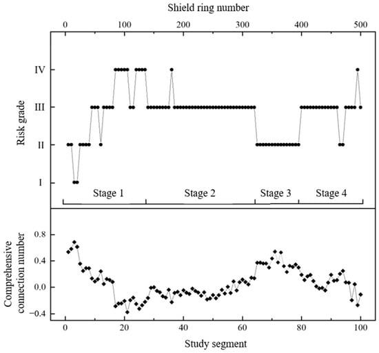
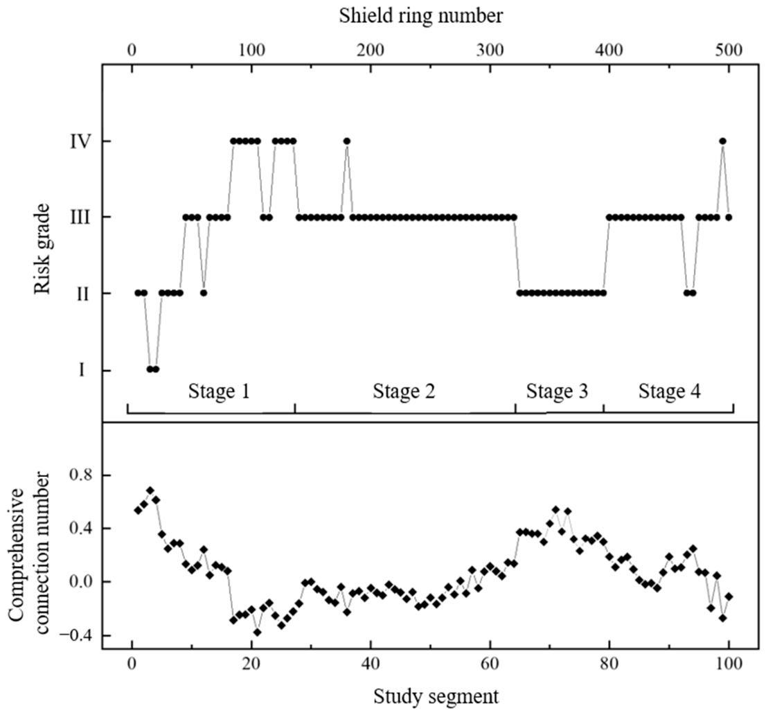
Based on the proposed risk assessment method, the comprehensive connection numbers and risk grades for the first 500 rings of the shield tunnel section were obtained. The assessment results and observed risk conditions are shown in Figure 3. As illustrated, the risk grades for the first 500 rings of the Hualong Station-Mingjingcun Shaft shield section fluctuate considerably, indicating an overall high safety risk level and substantial tunnelling risk.

Figure 3. Risk assessment results for the first 100 segments (Rings 1–500) of the shield tunnel.

The statistical results are summarised in Table 12. Grade I accounts for 2% of the evaluated segments, indicating safe tunnelling. Grade II accounts for 24%, corresponding to a “Relatively Safe” condition in which the indicator values are close to their standard values and tunnelling proceeds normally. Grade III accounts for 63%, corresponding to “Low Risk”, where the indicator values deviate from their standard values and tunnelling faces a certain degree of risk. Grade IV accounts for 11%, corresponding to “Moderately High Risk”, where the indicator values approach the boundary values and tunnelling faces considerable risk.

Table 12. Summary of risk assessment results for the first 100 segments (Rings 1–500).

Evaluation Segment	Risk Grade	Percentage
Segments 3–4	I	2%
Segments 1–2, 5–8, 12, 65–79, and 93–94	II	24%
Segments 9–11, 13–16, 22–23, 28–35, 37–64, 80–92, 95–98, and 100	III	63%
Segments 17–21, 24–27, 36, and 99	IV	11%

The geological conditions of the first 500 rings of the left-line section were relatively poor, and several problems occurred during construction, including multiple chamber interventions for cutter replacement. Based on the assessment results in Figure 3 and the actual engineering conditions, the risk evolution of the first 100 segments, corresponding to the first 500 rings, can be broadly divided into four stages as follows.

In Stage 1 (Segments 1–27), shield tunnelling commenced and proceeded mainly through completely weathered granite. The risk grade showed an increasing trend, rising from Grade I to Grade IV, with pronounced fluctuations. In Segments 24–27, the upper part of the excavation face consisted of silty clay, which is prone to softening and disintegration upon contact with water. Consequently, the risk is Grade IV.

In Stage 2 (Segments 28–64), the shield tunnel continued to advance mainly through alternating completely weathered and strongly weathered granite, where the geological conditions were relatively poor. The construction risk was predominantly Grade III, with occasional occurrences of Grade IV. Around Segment 36, moderately weathered granite appeared in the lower part of the tunnel section, resulting in upper-soft and lower-hard mixed ground and increasing the construction risk to Grade IV.

In Stage 3 (Segments 65–79), the shield tunnel continued to advance mainly through completely weathered granite, and all segments were classified as Grade II. In the later part of this stage, although the geological conditions remained poor, the risk grade did not increase, possibly because the shield operator selected appropriate tunnelling parameters and achieved effective risk control. For example, Segments 68–76 were all classified as Grade II; however, the corresponding connection numbers showed two adjustment cycles. When the connection number decreased and approached the threshold of Grade IV, the operator adjusted the tunnelling parameters, leading to a marked recovery in the connection number. This indicates that manual intervention effectively reduced the construction risk.

In Stage 4 (Segments 79–100), the shield machine advanced through upper-soft and lower-hard mixed ground under poor geological conditions. The construction risk was predominantly Grade III, reaching Grade IV at Segment 99.

3.2. Rings 501–1000

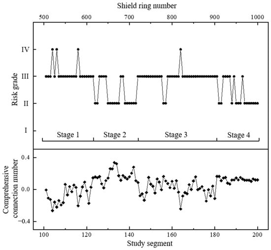
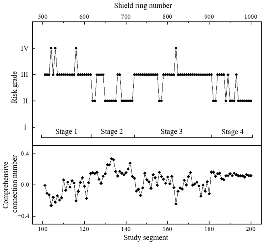
Through predictive risk assessment, the construction safety risks for Rings 501–1000 of the shield tunnel section were obtained, as shown in Figure 4. Compared with the first 500 rings, the risk grades for Rings 501–1000 fluctuate less markedly, indicating a generally lower risk level and more favourable engineering geological conditions.

Figure 4. Risk assessment results for segments 101–200 (Rings 501–1000) of the shield tunnel.

The statistical results are summarised in Table 13. Grade II accounts for 29% of the evaluated segments, corresponding to a “Relatively Safe” condition with normal tunnelling progress. Grade III accounts for 67%, corresponding to “Low Risk”, where the indicator values deviate from their standard values and tunnelling faces a certain degree of risk. Grade IV accounts for 4%, corresponding to “Moderately High Risk”, where the indicator values approach the boundary values and tunnelling faces considerable risk. No Grade I or Grade V risks were identified in the predictive assessment results for Rings 501–1000.

Table 13. Summary of risk assessment results for the latter 100 segments (Rings 501–1000).

Evaluation Segment	Risk Grade	Percentage
Segments 124–125, 130–135, 138–143, 156–157, 182–183, 188, 190–192, and 194–200	II	29%
Segments 101–103, 105, 107–115, 117–123, 126–129, 136–137, 144–155, 158–163, 165–181, 184–187, 189, and 193	III	67%
Segments 104, 106, 116, and 164	IV	4%

Based on the predictive risk assessment results shown in Figure 4 and the actual engineering conditions for Rings 501–1000, the risk evolution of the latter 100 segments can be broadly divided into four stages. In Stage 1 (Segments 101–123), the shield tunnel advanced alternately through full-face completely weathered granite and upper-soft and lower-hard mixed ground. The construction risk was predominantly Grade III, with occasional occurrences of Grade IV. In Stage 2 (Segments 124–143), the geological conditions were more favourable than those in Stage 1, and the construction risk was mainly Grade II. In Segments 126–129 and 136–137, silty clay occurred at the crown of the excavation face, causing the construction risk to increase to Grade III. In Stage 3 (Segments 144–181), the geological conditions were relatively poor, and the construction risk was predominantly Grade III. At Segment 164, the risk increased to Grade IV. In Stage 4 (Segments 182–200), the construction risk fluctuated mainly between Grade II and Grade III.

4. Discussions

The results show that construction risk in the investigated section was governed by the interaction between geological heterogeneity and shield operation, rather than by a single abnormal parameter. In the measured Rings 1–500, Grades III and IV accounted for 74% of the segments, including 11% at Grade IV. The risk was concentrated in sections where silty clay occurred near the crown while weathered or moderately weathered granite occupied the lower part of the face. This pattern is consistent with previous case studies showing that mixed-face conditions produce non-uniform cutting resistance, unbalanced cutterhead loading and unstable control requirements [6,7,8,9]. It also supports the observation that face-support parameters must be interpreted together with the ground type and groundwater conditions, rather than using a low or high pressure value as an isolated indication of safety [10].

The indicator results provide a mechanistic explanation for the identified high-risk segments. Cutterhead rotational speed, chamber pressure and total thrust were the most important parameters requiring attention in the representative assessment, and the same parameters repeatedly contributed to high local risk. In harder material at the lower face, insufficient or excessive rotational speed can increase cutting resistance, vibration and cutter wear; simultaneously, the thrust required to maintain advance changes with contact conditions at the soil–rock interface. Chamber pressure is directly related to face support and therefore influences both face stability and the possibility of ground loss. These mechanisms agree with reported relationships between construction parameters and settlement in soil–rock mixed faces [25] and with established analyses of EPB face stability [10]. The results therefore suggest that risk control should focus on coordinated parameter adjustment, rather than on maintaining each parameter within an independent fixed interval.

The evolution of the connection number also illustrates the value of treating risk as a continuous transition. In Segments 68–76, the grade remained at Grade II after two adjustment cycles, although the connection number first approached the Grade IV boundary and subsequently recovered. This behaviour indicates that the connection number can provide an earlier warning of deterioration than a discrete grade alone. It is consistent with the broader development of shield-monitoring methods, in which operational records are linked with ground displacement, geological information or anomaly detection [23,24,26,27]. In practice, a decreasing connection number should trigger a re-view of cutterhead speed, thrust, chamber pressure, advance rate and face conditions; the final intervention decision should then be checked against deformation monitoring and construction observations. Operational data are informative proxies for changing ground conditions, but they do not replace independent evidence of ground response [23,25].

The coupled weighting and fuzzy set pair analysis framework offers two complementary advantages. First, combining AHP and the coefficient-of-variation method prevents the assessment from relying exclusively on either expert perception or sample dispersion. This is important because an indicator can have modest global importance while exhibiting a severe local exceedance. Second, the five-element connection number and triangular fuzzy coefficients preserve the gradual identity–discrepancy–contrary transition around grade boundaries. Compared with rigid threshold classification, this formulation is better suited to tunnelling, where a small change in geological condition or operating state rarely produces an instantaneous change from safe to unsafe. The approach complements Bayesian, event-tree, fuzzy-AHP and cloud-model methods reported for tunnel risk assessment [15,16,17,18,19,20,21,22,29,30,31,32,33,34]. Its main contribution is an interpretable segment-level output that links a risk grade to the individual operational indicators that produced it.

The comparison between the two 500-ring sections should, however, be interpreted with care. The later section contains 29% Grade II, 67% Grade III and 4% Grade IV segments, compared with 24%, 63% and 11% for the measured first section. The smaller proportion of Grade IV and the smoother profile are compatible with the more favourable geological description, but Rings 501–1000 were represented by predicted rather than measured inputs. A lower predicted risk therefore indicates the modelled tendency under the supplied inputs, not an independent validation of safer construction. Recent prediction and early-warning studies likewise distinguish forecasting performance from risk-state verification and stress the importance of combining operational, stratigraphic and monitoring data [26,27,28]. Future applications should report prediction errors and confidence intervals, propagate input uncertainty through the fuzzy connection number, and update the assessment when actual ring-level observations become available.

Several limitations define the current scope of the findings. The case study concerns one tunnel section and one EPB machine, the weights are fixed for the analysed dataset, and the five-ring aggregation may smooth short-lived abnormalities. The expert weighting also relies on nine valid responses, while deformation, groundwater and cutter-wear observations were not included as independent indicators. Accordingly, the proposed grades should be used as decision-support information rather than as a substitute for engineering judgement or statutory monitoring. A broader validation programme should include multiple projects and geological settings, sensitivity analysis of the weighting and grade boundaries, adaptive or time-varying weights, and multi-source fusion with settlement, face-pressure and geological observations. These extensions would improve transferability while retaining the model’s practical advantage of identifying high-risk segments and the parameters most suitable for immediate control.

5. Conclusions

This study developed a coupled subjective–objective weighting and fuzzy set pair analysis model to assess the construction risk of shield tunnelling in upper-soft and lower-hard mixed ground. The proposed method was validated using tunnelling data. Based on the theoretical formulation and engineering application, the following conclusions can be drawn.

(1) A coupled risk assessment model integrating subjective–objective weighting and fuzzy set pair analysis was developed for shield tunnelling in upper-soft and lower-hard mixed ground. By combining AHP with the coefficient of variation method, the model incorporates both expert engineering judgement and the statistical variability of field tunnelling data, providing a more balanced basis for determining indicator weights.

(2) The five-element connection number and segmented triangular fuzzy numbers enable a refined description of the gradual transition among risk grades. This treatment reduces the rigidity of conventional grade-boundary classification and allows the identity, discrepancy and contrary relationships between tunnelling parameters and risk standards to be quantified more effectively.

(3) The application to the Hualong Station-Mingjingcun Shaft section demonstrates that the proposed model can capture the risk evolution of shield tunnelling in mixed ground. For Rings 1–500, the risk grades fluctuate markedly and are mainly Grade II-III, with local Grade IV risks associated with poor geological conditions and parameter abnormalities. For Rings 501–1000, the predicted risk level is relatively lower and more stable, indicating more favourable geological conditions and controllable construction risk.

(4) The case study shows that cutterhead rotational speed, chamber pressure and total thrust are key parameters requiring particular attention during construction. The proposed assessment procedure provides a quantitative and practical tool for identifying high-risk segments and supporting targeted risk control in shield tunnelling through heterogeneous strata.

Future work will proceed along four complementary directions. First, the framework will be externally validated using measured ring-level data from multiple shield projects, EPB machines and mixed-ground settings to examine the transferability of the indicator weights and grade boundaries. In particular, the predicted inputs for Rings 501–1000 will be replaced by field measurements as they become available, allowing prediction errors and their propagation into the risk grades to be quantified. Second, the indicator system will be expanded by integrating geological and groundwater information with surface and structural deformation, cutter wear and other construction-response data. Sensitivity and uncertainty analyses will then be used to identify robust indicators and thresholds. Third, adaptive or time-varying weights and rolling model updating will be investigated so that the assessment can respond to changes in ground conditions and machine behaviour rather than relying on fixed weights throughout the alignment. Finally, the model will be incorporated into a real-time early-warning prototype linked to the shield control platform. Field trials will evaluate warning lead time, false-alarm frequency and the effectiveness of parameter-adjustment recommendations, thereby supporting the transition from retrospective segment classification to operational risk control.

References

- Maidl, B.; Herrenknecht, M.; Maidl, U.; Wehrmeyer, G. Mechanised Shield Tunnelling, 2nd ed.; Ernst & Sohn: Berlin, Germany, 2012. [Google Scholar]
- Guglielmetti, V.; Grasso, P.; Mahtab, A.; Xu, S. Mechanized Tunnelling in Urban Areas: Design Methodology and Construction Control; Taylor & Francis: London, UK, 2008. [Google Scholar]
- Chapman, D.; Metje, N.; Stark, A. Introduction to Tunnel Construction, 2nd ed.; CRC Press: London, UK, 2017. [Google Scholar]
- Chen, W.T.; Han, K.H.; Zhou, J. Settlement response of existing metro tunnels induced by parallel symmetric shield tunneling: A model test study. Buildings 2026, 16, 2555. [Google Scholar] [CrossRef] [Scilit]
- Wang, J.R.; Zhang, L.Y.; Zhang, H.M.; Ding, X.H.; Luo, B. Deformation and control of bridge pile adjacent to excavation under superimposed disturbances of shield tunneling and the top-down method. Buildings 2026, 16, 2879. [Google Scholar] [CrossRef] [Scilit]
- Zhao, J.; Gong, Q.M.; Eisensten, Z. Tunnelling through a frequently changing and mixed ground: A case history in Singapore. Tunn. Undergr. Space Technol. 2007, 22, 388–400. [Google Scholar] [CrossRef] [Scilit]
- Steingrimsson, J.H.; Grov, E.; Nilsen, B. The significance of mixed-face conditions for TBM performance. World Tunn. 2002, 15, 435–441. [Google Scholar]
- Bilgin, N.; Copur, H.; Balci, C. Mechanical Excavation in Mining and Civil Industries; CRC Press: Boca Raton, FL, USA, 2014. [Google Scholar]
- Toth, A.; Gong, Q.M.; Zhao, J. Case studies of TBM tunneling performance in rock–soil interface mixed ground. Tunn. Undergr. Space Technol. 2013, 38, 140–150. [Google Scholar] [CrossRef] [Scilit]
- Anagnostou, G.; Kovari, K. Face stability conditions with earth-pressure-balanced shields. Tunn. Undergr. Space Technol. 1996, 11, 165–173. [Google Scholar] [CrossRef] [Scilit]
- Einstein, H.H. Risk and risk analysis in rock engineering. Tunn. Undergr. Space Technol. 1996, 11, 141–155. [Google Scholar] [CrossRef] [Scilit]
- Sturk, R.; Olsson, L.; Johansson, J. Risk and decision analysis for large underground projects, as applied to the Stockholm Ring Road tunnels. Tunn. Undergr. Space Technol. 1996, 11, 157–164. [Google Scholar] [CrossRef] [Scilit]
- Reilly, J.J. The management process for complex underground and tunneling projects. Tunn. Undergr. Space Technol. 2000, 15, 31–44. [Google Scholar] [CrossRef] [Scilit]
- Eskesen, S.D.; Tengborg, P.; Kampmann, J.; Veicherts, T.H. Guidelines for tunnelling risk management: International Tunnelling Association, Working Group No. 2. Tunn. Undergr. Space Technol. 2004, 19, 217–237. [Google Scholar] [CrossRef] [Scilit]
- Sousa, R.L.; Einstein, H.H. Risk analysis during tunnel construction using Bayesian networks: Porto Metro case study. Tunn. Undergr. Space Technol. 2012, 27, 86–100. [Google Scholar] [CrossRef] [Scilit]
- Hong, E.S.; Lee, I.M.; Shin, H.S.; Nam, S.W.; Kong, J.S. Quantitative risk evaluation based on event tree analysis technique: Application to the design of shield TBM. Tunn. Undergr. Space Technol. 2009, 24, 269–277. [Google Scholar] [CrossRef] [Scilit]
- Hyun, K.C.; Min, S.; Choi, H.; Park, J.; Lee, I.M. Risk analysis using fault-tree analysis (FTA) and analytic hierarchy process (AHP) applicable to shield TBM tunnels. Tunn. Undergr. Space Technol. 2015, 49, 121–129. [Google Scholar] [CrossRef] [Scilit]
- Saaty, T.L. A scaling method for priorities in hierarchical structures. J. Math. Psychol. 1977, 15, 234–281. [Google Scholar] [CrossRef] [Scilit]
- Zadeh, L.A. Fuzzy sets. Inf. Control 1965, 8, 338–353. [Google Scholar] [CrossRef] [Scilit]
- Zadeh, L.A. The concept of a linguistic variable and its application to approximate reasoning—I, II, III. Inf. Sci. 1975, 8, 199–249. [Google Scholar] [CrossRef] [Scilit]
- Li, D.Y.; Liu, C.Y.; Gan, W.Y. A new cognitive model: Cloud model. Int. J. Intell. Syst. 2009, 24, 357–375. [Google Scholar] [CrossRef] [Scilit]
- Nezarat, H.; Sereshki, F.; Ataei, M. Ranking of geological risks in mechanized tunneling by using fuzzy analytical hierarchy process (FAHP). Tunn. Undergr. Space Technol. 2015, 50, 358–364. [Google Scholar] [CrossRef] [Scilit]
- Jiang, H.; Cheng, J.; Zhang, J.; Zhang, J.; Su, Y.; Zheng, Y. Principle and application of in-situ monitoring system for ground displacement induced by shield tunnelling. Tunn. Undergr. Space Technol. 2021, 112, 103905. [Google Scholar] [CrossRef] [Scilit]
- Yan, T. Data on prediction of geological characteristics during shield tunnelling in mixed soil and rock ground. Data Brief 2022, 45, 108726. [Google Scholar] [CrossRef] [Scilit] [PubMed]
- Guo, S.; Wang, B.; Zhang, P.; Wang, S.; Guo, Z.; Hou, X. Influence analysis and relationship evolution between construction parameters and ground settlements induced by shield tunneling under soil-rock mixed-face conditions. Tunn. Undergr. Space Technol. 2023, 134, 105020. [Google Scholar] [CrossRef] [Scilit]
- Loy-Benitez, J.; Lee, H.K.; Song, M.K.; Lee, J.K.; Lee, S.S. Real-time unsupervised monitoring of earth pressure balance shield-induced sinkholes in mixed-face ground conditions via convolutional variational autoencoders. Tunn. Undergr. Space Technol. 2024, 152, 105908. [Google Scholar] [CrossRef] [Scilit]
- Deng, L.C.; Zhang, W.; Deng, L.; Shi, Y.H.; Zi, J.J.; He, X.; Zhu, H.H. Forecasting and early warning of shield tunnelling-induced ground collapse in rock-soil interface mixed ground using multivariate data fusion and Catastrophe Theory. Eng. Geol. 2024, 335, 107548. [Google Scholar] [CrossRef] [Scilit]
- Hu, M.; Cheng, P. Long-Distance Shield Tunnelling Performance Prediction Based on Informer. Appl. Sci. 2025, 15, 1674. [Google Scholar] [CrossRef] [Scilit]
- Chung, H.; Park, J.; Kim, B.K.; Kwon, K.; Lee, I.M.; Choi, H. A Causal Network-Based Risk Matrix Model Applicable to Shield TBM Tunneling Projects. Sustainability 2021, 13, 4846. [Google Scholar] [CrossRef] [Scilit]
- Guo, D.S.; Meng, F.Y.; Wu, H.N.; Yang, X.X.; Liu, Z. Risk assessment of shield tunneling crossing building based on variable weight theory and cloud model. Tunn. Undergr. Space Technol. 2024, 145, 105593. [Google Scholar] [CrossRef] [Scilit]
- Chen, H.; Shen, G.Q.; Feng, Z.; Yang, S. Safety risk assessment of shield tunneling under existing tunnels: A hybrid trapezoidal cloud model and Bayesian network approach. Tunn. Undergr. Space Technol. 2024, 152, 105936. [Google Scholar] [CrossRef] [Scilit]
- Chen, Y.L.; Shen, S.L.; Zhou, A.; Zeng, Y. Novel model for evaluating ground settlement risk in slurry balance shield tunnel construction. Tunn. Undergr. Space Technol. 2024, 150, 105853. [Google Scholar] [CrossRef] [Scilit]
- Guo, D.; Meng, F.; Wu, H.; Yang, X.; Chen, R. Risk assessment of shield construction adjacent to the existing shield tunnel based on improved nonlinear FAHP. Tunn. Undergr. Space Technol. 2025, 155, 106154. [Google Scholar] [CrossRef] [Scilit]
- Sun, X.; Wu, L.; Wu, D. Risk evaluation of metro tunnel shield construction based on game variable weight extension cloud theory. Sci. Rep. 2025, 15, 18961. [Google Scholar] [CrossRef] [Scilit] [PubMed]
Disclaimer/Publisher’s Note: The statements, opinions and data contained in all publications are solely those of the individual author(s) and contributor(s) and not of MDPI and/or the editor(s). MDPI and/or the editor(s) disclaim responsibility for any injury to people or property resulting from any ideas, methods, instructions or products referred to in the content. |
© 2026 by the authors. Licensee MDPI, Basel, Switzerland. This article is an open access article distributed under the terms and conditions of the Creative Commons Attribution (CC BY) license.