


Abstract
Against the backdrop of global energy conservation and emission reduction strategies, university teaching buildings are key targets for carbon emission management due to their multifunctional characteristics and distinct usage patterns. To address the limitations of conventional prediction models in capturing dynamic characteristics of hourly operational carbon emission, a teaching building cluster at a university in Guangzhou was selected as the case study. Hourly occupancy, meteorological data, and electricity consumption data were integrated. A baseline long short-term memory (LSTM) model and seven hybrid deep learning models were developed. The predictive performance of the models was systematically compared using the one-year and two-year training datasets. The results show that the data scale significantly affects the model’s applicability. Under the one-year dataset, the weekly seasonal naive baseline model achieves the best overall reference performance. In the deep learning models, the CNN-ATT-LSTM model performs best in trend fitting and absolute error control, while the CNN-LSTM model shows more balanced performance in relative error control and repeated training stability. At the same time, the CNN-ATT-LSTM model achieves a better balance between prediction performance and computational efficiency. Under the two-year dataset, the CNN-LSTM model exhibits optimal overall performance across all prediction accuracy indicators and achieves the most favorable balance between prediction accuracy and computational cost. Further analysis indicates that model performance does not monotonically increase with increasing model complexity. Therefore, the model structure should be matched with the available data basis and specific application requirements. The research results can serve as a basis for model selection for short-term carbon emission prediction in university teaching buildings and provide technical support for improving carbon emission management in these buildings.
1. Introduction
In recent years, the rapid growth in global energy consumption and carbon emission has accelerated climate change. Guided by the goals of carbon peaking and carbon neutrality, energy conservation and emission reduction are of great concern today. The United Nations Intergovernmental Panel on Climate Change (IPCC) released a report stating that by 2100, excessive greenhouse gas emission will cause global average temperature to rise by 1.8 to 4 degrees Celsius [1]. In urban areas, the growing frequency of summertime extreme heat events has increased public willingness to support heat mitigation and adaptation measures [2], while the synergistic risks of extreme heat and air pollution have posed increasing threats to urban residents [3]. According to statistics from the United Nations Environment Programme (UNEP), the construction industry accounts for approximately 30 to 40 percent of global energy consumption and greenhouse gas emission, making it one of the primary sources of carbon emission [4]. Against the backdrop of increasingly stringent emission reduction requirements in the construction sector, universities are complex public buildings that integrate teaching, research, office functions, and residential services. Their large scale, functional diversity, and high occupancy contribute to an overall upward trend in operational energy consumption and carbon emission. Teaching buildings are used frequently, and their carbon emission is affected by course schedules, examination periods, holidays, weather conditions, and occupant mobility. Consequently, emission patterns fluctuate and exhibit periodicity across daily, weekly, and semester time scales, which limits the ability of static accounting methods to accurately represent actual operating conditions. Short-term carbon emission forecasting for university teaching buildings can therefore support the identification of emission patterns, the assessment of carbon effects associated with air conditioning and lighting control measures, and the optimization of building operation strategies.
Currently, in the field of building carbon emission forecasting, scholars have proposed various forecasting methods and techniques. Most of these methods focus on analyzing the dominant factors influencing carbon emission and using them as the basis for developing various forecasting models [5]. These can be broadly categorized into physical modeling and data-driven modeling methods [6]. Physical modeling methods use information on functional building zones, envelope and façade configurations, and material and construction characteristics to develop numerical building models using energy simulation tools such as EnergyPlus [7], DeST [8], and TRNSYS [9]. The process of building and solving the model for this method is relatively complex, requires a large number of model parameters and input data, and is computationally intensive and time-consuming.
Unlike physics-based models, which rely on mechanistic analysis, data-driven models are primarily based on historical sample data. They use methods such as statistical analysis and machine learning to establish input–output relationships between building carbon emission and relevant influencing factors, thereby enabling the prediction of carbon emission levels. Since these models do not require a complete description of complex physical processes within building systems, their advantages in efficiency, computational cost, and applicability have made this approach essential for predicting building carbon emission. Based on differences in modeling approaches, data-driven models can be broadly categorized into two types: traditional statistical models, which primarily include factor decomposition models based on the Kaya identity, the TIRPAT model, and various regression models; and intelligent forecasting models, represented by machine learning and neural networks. The latter can capture the nonlinear characteristics of carbon emission data to a certain extent and can be used in conjunction with multivariate information to conduct predictive analysis. As a result, it remains widely used in research on building energy consumption forecasts.
However, the predictive performance of data-driven models is typically closely related to the dimensions, quality, and sample size of the input data, a focus of much existing research. Particularly in predicting carbon emission from building operations, the relevant data are influenced not only by the combined effects of multiple factors but also often exhibit fluctuations over time. Therefore, in addition to describing the nonlinear relationships among variables, the model must also capture the characteristics of time-series data. Based on this, deep learning models suitable for time series forecasting, including Deep Neural Network (DNN), Recurrent Neural Network (RNN), and Convolutional Neural Network (CNN), have gradually garnered attention. Among these, the Long Short-Term Memory (LSTM) is a variant of RNN and is well-suited for processing long data sequences. It can mitigate the vanishing gradient and exploding gradient problems that may arise during the training of a traditional RNN. As a result, it has been widely adopted in building carbon emission forecasting. In short-term forecasting scenarios, such as building heat loads, it also demonstrates certain advantages in terms of forecasting accuracy and robustness [10]. In addition, carbon emission from university teaching buildings during the operational phase are influenced by a combination of factors, including occupancy levels, spatial characteristics, and meteorological conditions, and typically exhibit distinct cyclical and regular fluctuations [11]. Against this backdrop, the LSTM model is well-suited for such scenarios. In particular, it can preserve historical information across long time series, especially cross-week patterns arising from different operational modes such as classes, exams, and holidays. Existing research also supports this conclusion. Zhou et al. used an LSTM model to predict short-term energy consumption for a library air conditioning system. The results showed that the LSTM model achieved lower values for evaluation metrics, including root mean square error (RMSE), Mean Absolute Deviation (MAD), and mean absolute percentage error (MAPE), than traditional mathematical prediction models [12]. Wang et al. compared various shallow and deep learning forecasting methods using heat load data from a mixed-use university campus building. They found that LSTM performed better overall in short-term energy consumption forecasting [10].
Because single deep learning models have limitations in terms of predictive accuracy and robustness, some researchers have developed improved or hybrid LSTM-based models to enhance their predictive performance. Wu et al. used a CNN-LSTM model to extract spatiotemporal features of building energy consumption and, by incorporating a model transfer strategy, improved the accuracy of building energy consumption predictions in the target domain under few-data-point conditions [13]. Lu et al. developed a hybrid precision gradient accumulation framework based on CNN-LSTM to explore energy-efficiency optimization methods for spatiotemporal modeling of sports venues [14]. Fan et al. developed an interpretable energy consumption prediction model based on a CNN-LSTM to explore methods for predicting energy consumption in building cooling and air conditioning systems and to identify key features [15]. Verma et al. developed a model combining an LSTM with an Attention Mechanism (ATT) to compare carbon emission prediction performance and to evaluate carbon footprint assessment methods during training [16]. Jiang et al. introduced correlation filtering and attention mechanisms based on LSTM-ATT to explore methods for predicting energy consumption during building operation [17]. Zhang et al. developed a model for predicting energy consumption in public buildings by integrating CNN, LSTM, and ATT to combine CNN-based feature extraction with attention mechanisms. They validated its high accuracy [18].
Currently, there remains a lack of systematic evaluation of LSTM-based approaches for short-term carbon emission forecasting in university teaching buildings. Existing occupancy data have low temporal resolution and therefore fail to adequately capture key drivers such as class schedules, exam weeks, and self-study behavior. In addition, prediction errors, trend stability, and model generalization capabilities across different data scales have received insufficient attention. Given that carbon emission from university teaching buildings exhibit both cross-period dependencies and high-frequency local fluctuations, this research develops and compares an LSTM model with an improved model that integrates CNN and attention mechanisms. Specifically, LSTM is used to capture the long-term sequence structure formed by course schedules and exam cycles, while CNN is employed to extract local variations caused by activities such as class sessions and mass dismissal. This research further evaluates model accuracy, sensitivity to data volume, and computational cost to provide a basis for deployment during the operational phase.
Given the shortcomings of the existing research discussed above, this research addresses the following areas:
- Based on the usage characteristics of educational buildings and the patterns of educational activities, and taking into account course schedules and field survey data, an hourly occupancy sequence was developed. This sequence, along with hourly meteorological and carbon emission data, was used as model input to enhance its ability to characterize the temporal operational patterns of educational buildings.
- Under uniform hyperparameter settings and training strategies, a systematic comparative analysis of the predictive performance of the baseline LSTM and its seven hybrid models was conducted.
- Evaluate the suitability of each model based on two dimensions, namely training data scale and computational cost, and propose model selection and deployment recommendations tailored to different data conditions and management requirements.
The framework of this research is shown in Figure 1. First, this research integrates actual hourly electricity-consumption data and hourly occupancy information from university teaching buildings with hourly meteorological data from the CSWD. Carbon emission during the building operation phase was calculated using the emission factor method, and meteorological variables with relatively large absolute Spearman correlation coefficients were selected to construct the prediction dataset. Subsequently, this research performs data preprocessing through missing-value handling, dataset splitting, normalization, and sliding-window transformation. Using LSTM as the baseline model, this research constructs hybrid prediction models by combining CNN and attention mechanisms. It optimizes hyperparameters, including the learning rate, number of training iterations, batch size, optimizer, and activation functions. Finally, this research conducts repeated experiments using one-year and two-year datasets and averages the results. The predictive performance and computational efficiency of each model are comprehensively evaluated using the coefficient of determination (R2), root mean square error (RMSE), mean absolute error (MAE), mean absolute percentage error (MAPE), and computational cost (t). Based on these results and the actual operational characteristics of university teaching buildings, this research proposes recommendations for model selection.
Figure 1.
Research framework.
2. Materials and Methods
2.1. Study Object
The subject of this research is a complex of academic buildings at a university in Guangzhou, Guangdong Province, located in a region characterized by hot summers and mild winters. This building complex consists of standard classroom buildings for public educational use. The primary building activities are routine teaching operations and do not include specialized teaching spaces such as laboratories or mechanical and electrical training rooms. This eliminates additional energy consumption interference caused by specialized experimental equipment, allowing this research better to reflect the operational characteristics of typical educational buildings. The complex comprises four teaching buildings arranged in a courtyard layout, connected by skywalks. The enclosed outdoor courtyard facilitates the inflow of natural breezes, while the complex is oriented 23° west of north and features a reinforced concrete frame structure. The two buildings on the south side are five stories tall, each measuring 25.45 m, while the two on the north side are four stories tall, each measuring 24.10 m. The total floor area is approximately 38,000 m2, with no underground space. The outdoor courtyard enclosed by the buildings facilitates the flow of natural breezes.
In actual use, the building’s primary function is as an educational space, equipped with office areas including faculty lounges, an examination office, and seminar rooms. There are five offices in total, primarily located on the first and fifth floors of Building A and on the second floor at the junctions between the individual buildings. Staff activity patterns follow normal working hours, with staff on duty during holidays. In addition, there are 111 classrooms in total. Among these, the five classrooms on the first, second, and third floors of Building C are designated as self-study rooms for students only. They are rarely used for classes or exams and are open daily from 8:00 a.m. to 10:00 p.m. during the semester.
Based on an on-site survey, this building complex is open in its entirety to faculty and students during regular academic hours throughout the semester (including weekdays and weekends). For energy-saving and management purposes, during all public holidays and winter and summer breaks, only the five self-study rooms on the first, second, and third floors of Building C remain open daily for students’ independent study.
2.2. Dataset Construction
2.2.1. Hourly Carbon Emission Data
Carbon emission during the operational phase of a building may originate from direct fuel combustion and indirect emission associated with purchased electricity and heat. The educational building complex investigated in this research has no on-site combustion equipment, district heating demand, or renewable energy generation system. Its operational energy consumption is primarily electricity for lighting, air conditioning, and auxiliary equipment. Therefore, the operational carbon emission boundary is limited to indirect carbon emission associated with electricity purchased from the grid. Direct emission from on-site fuel combustion, embodied carbon emission from construction materials, and carbon emission associated with building construction, maintenance, and demolition are outside the defined scope.
Currently, three main methods are commonly used in China for quantifying carbon emission: the direct measurement method, the mass balance method, and the carbon emission factor method [19]. A comprehensive comparison of these three methods reveals that the direct measurement method is limited to direct carbon emission. In contrast, the mass balance method often makes it difficult to account for carbon substances because of the large number of input and output material types, which typically have unstable carbon content. The carbon emission factor method requires only two parameters and is widely used in construction projects. Therefore, the carbon emission factor method was ultimately selected for carbon emission calculations:
where is the indirect carbon emission from electricity purchases during the building’s operation phase at time t; Eelec,t is the electricity purchase volume for the building at time t; EFelec is the carbon emission factor of electricity; is the cumulative carbon emission volume within the time interval [t1,t2].
Specifically, hourly operational carbon emission was calculated by multiplying the building complex’s hourly electricity consumption by the electricity carbon emission factor. Based on data from the “Announcement on the Release of 2023 Electricity Carbon Dioxide Emission Factors” issued on 31 December 2025, by the Ministry of Ecology and Environment of the People’s Republic of China and the National Bureau of Statistics of China, the electricity carbon emission factor used in this research is 0.4419 kgCO2e/kWh. The resulting target variable represents the building complex’s hourly indirect operational carbon emission, expressed in kgCO2e/h. The emission factor is applied to purchased grid electricity and represents the corresponding indirect emission under the adopted electricity accounting boundary. It does not represent direct fuel-combustion emission or embodied carbon emission.
For this research, hourly electricity consumption data for this group of academic buildings from 1 January 2024 to 31 December 2025 were obtained from the Campus General Affairs Office, and hourly carbon emission was calculated using the carbon emission-factor method.
2.2.2. Hourly Meteorological Data
Given the location of this educational building complex, this research used Chinese Standard Weather Data (CSWD) to obtain meteorological data for the corresponding grid area for 2024 and 2025, including variables that may influence carbon emission during the building’s operational phase. The data include hourly outdoor dry-bulb temperature, dew-point temperature, relative humidity, direct solar radiation, diffuse horizontal radiation, and wind speed. This dataset provides meteorological variables for this research area at an hourly resolution.
In developing a carbon emission prediction model, feature-selection methods are required to remove meteorological variables with low correlations, thereby increasing the proportion of useful information in the original data, reducing computational load, and improving the model’s generalization. In this research, Spearman correlation analysis was performed for each variable, and the resulting heatmap is presented in Figure 2. Subsequently, dry-bulb temperature, dew point temperature, diffuse horizontal irradiance, and hourly number of occupants, which had the highest absolute correlation coefficients, were selected as meteorological features.
Figure 2.
Spearman correlation coefficients for each input feature.
2.2.3. Hourly Occupancy Data
To construct a time series of occupancy data for the academic building complex throughout the year, indoor occupancy information was categorized into two types, namely academic management data and on-site observation data, based on the methods used to collect the data, and these data were then integrated under a unified time scale. The on-site survey results indicate that the primary users of this complex are students and staff. Student activities primarily consist of classes, examinations, and self-study, while staff members mainly include faculty, administrative personnel, and support staff. For activities subject to strict scheduling constraints, such as classes and examinations, the course and examination schedules for the four semesters spanning the 2024–2025 academic year were obtained from the campus Academic Affairs Office. This information was then mapped to specific hourly time slots based on the university’s standardized class schedule, thereby generating hourly planned occupancy data. Based on the academic calendar, each semester generally consists of 19 or 20 weeks, with the final two weeks typically designated as examination weeks, while regular instruction is primarily distributed across weeks 1 through 17 or 18. Since the number of students scheduled for a class does not fully reflect actual classroom attendance, attendance rates were applied to adjust the student counts for each class period. Existing research indicates that there is approximately a 20% discrepancy between occupancy forecasts derived from classroom scheduling systems and actual attendance figures [20]. Another study, which combined surveillance video frames, a Multi-Column Convolutional Neural Network (MCNN), Context-Aware Crowd Counting (CAN), and timetable analysis, found that the average actual attendance rate in university classrooms is approximately 77% [21]. Based on this finding, the number of students attending classes was adjusted to reflect a 77% attendance rate. In contrast, the number of students during examination periods was counted as full attendance, thereby yielding hourly occupancy data for both classes and examinations.
For students studying on their own and staff members, on-site observation methods were used to supplement the data due to the lack of directly accessible management data. Given that occupancy in this area is significantly influenced by factors such as the academic calendar, holiday schedules, winter and summer breaks, and building access status, the year was first divided into six categories based on the academic calendar and the university’s operational characteristics: academic weeks, the two weeks preceding exam weeks, exam weeks, public holidays, and winter and summer breaks. Among these, academic weeks, the two weeks preceding exam weeks, and exam weeks were further subdivided into weekdays and weekends, whereas public holidays primarily refer to China’s statutory holidays. Based on this framework, hourly on-site surveys were conducted for each scenario to identify corresponding typical usage patterns. This research was conducted through on-site data collection in 2026 from 4–9 April, 11–12 April, and 18 April (a total of 9 days, including public holidays, working days, and weekends). Room-by-room counts were performed at 1 h intervals from 6:00 a.m. to 11:00 p.m. each day. A total of 162 sets of self-study occupancy records were obtained over the nine days, and the average values for each time slot were used to establish the occupancy sequence for the public holiday scenario. Staff occupancy data was also obtained through on-site counting and organized into three categories: during the academic term, winter and summer break, and holidays. Within the academic term, winter and summer breaks, data were broken down by weekday and weekend to characterize changes in staff presence across different operational phases.
During data construction, occupancy data from various sources were mapped and fused using the hour as a uniform time scale. For on-site observation results, hourly averages across multiple survey days under the same conditions were used to reduce random fluctuations in individual observations. Subsequently, based on the annual academic calendar, class sessions, exams, self-study periods, and staff occupancy were assigned to corresponding dates and time slots, ultimately generating hourly occupancy data for the building throughout the year. Although manual tabulation may introduce some error, the resulting occupancy data can effectively reflect the temporal variation in building occupancy and meet the requirements for subsequent model training, given the comprehensive coverage of the survey periods, the relatively ample number of repeated samples, and the relative stability of occupancy patterns under similar conditions. The complete dataset is shown in Figure 3.
Figure 3.
Building carbon emission data, building occupancy data and hourly meteorological data.
2.3. Data Preprocessing
The preprocessing of the original dataset consisted of four steps: handling missing data, data partitioning, data standardization, and sliding window processing.
2.3.1. Missing Data Handling
The original data used in this research consists of cumulative electricity consumption readings from 80 sub-meters in the case study building. The recording period spans from 00:00 on 1 January 2024 to 24:00 on 31 December 2025, with a theoretical sampling interval of 15 min. The data presents two issues: First, meter readings are missing for certain time points. Second, a small number of observations do not strictly fall at standard 15 min intervals but are instead scattered across adjacent 1 min time points, exhibiting certain complementary characteristics across different meter dimensions.
Given the characteristics described above, this research first constructs a 1 min continuous-time index and uses a forward-filling method to time-align the cumulative electricity consumption time series. Subsequently, data are extracted at 15 min intervals to reconstruct a unified cumulative electricity consumption time series. Based on this, the electricity consumption for each meter’s 15 min interval was calculated by taking the difference between adjacent time points. Minor positive values greater than 0 but less than 0.01 were treated as noise and uniformly recorded as missing values, while intervals with a difference of 0 were retained as zero load. Finally, the restored 15 min electricity consumption data is aggregated by the hour to generate a time series of the building’s total hourly electricity consumption, providing data support for subsequent energy consumption analysis and predictive modeling.
2.3.2. Data Partitioning
To ensure the model’s generalization and evaluate its predictive performance, this research divided the dataset into a training set, a validation set, and a test set in chronological order. The one-year dataset covers from 1 January 2025, to 31 December 2025, totaling 8760 samples. The two-year dataset covers from 1 January 2024, to 31 December 2025, totaling 17,544 samples. Both datasets use the same test interval, from 7 November 2025, to 31 December 2025, to ensure consistency in model performance comparisons. In the one-year dataset, the training set accounts for 70.00% and corresponds to the period from 1 January 2025, to 13 September 2025. The validation set accounts for 15.00% and corresponds to the period from 13 September 2025, to 7 November 2025. In the two-year dataset, the training set accounts for 76.18% and corresponds to the period from 1 January 2024, to 10 July 2025. The validation set accounts for 16.33% of the period from 10 July 2025, to 7 November 2025.
2.3.3. Data Normalization
After completing the data partitioning, the input features were transformed using a robust scaling method based on the median and interquartile range calculated from the training set. The target variable was processed using the same robust scaling strategy during model training and was transformed back to its physical scale before calculating the evaluation metrics.
2.3.4. Sliding Window Processing
This research employs a multi-input, single-step forecasting method with a sliding window length of 168 and a sliding step size of 1. Specifically, in the t-th sliding window, historical hourly operational carbon emission data for time steps (t, t − 1, …, t − 167) and other feature data are input into the forecasting model to predict the hourly indirect operational carbon emission at time t + 1. The window then slides forward by one time step along the time series, and the above process is repeated until the entire time series dataset has been traversed. Since each input window contains only historical observations obtained before the prediction time, data at time t + 1 and beyond are not included in the input window. Therefore, the model cannot access information about the target prediction time and future time points during the training, validation, and testing phases. Thus, the role of BiLSTM in this study is to perform bidirectional encoding of available historical information, rather than relying on future observations for prediction. The number of slides required for data preprocessing using sliding time windows across the entire time series:
where KSW is the total number of sliding steps; M is the total length of the data; nSW is the length of the sliding window; SSW is the sliding step size.
2.4. Model Principles
2.4.1. Long Short-Term Memory Neural Network
To address issues in RNN, such as the loss of long-term dependencies, vanishing gradients, and exploding gradients, Hochreiter et al. proposed LSTM model based on RNN [22]. As shown in Figure 4, LSTM incorporates a hidden gate structure consisting of a forget gate, an input gate, and an output gate into the RNN architecture [23]. This structure enables the selective retention and removal of historical information, thereby allowing the model to capture both long-term and short-term sequence dependencies.
Figure 4.
The structure of LSTM.
- The Forgetting Gate (f_t) uses the input at the current time step and the hidden state from the previous time step to determine the amount of information to be forgotten from the cell’s memory unit at the previous time step. It generates a forgetting vector between 0 and 1 using a sigmoid function and multiplies it pointwise with the previous cell state to filter the information:
ft = σ(Wf[ht−1,xt] + bf)
- 2.
- The input gate (it) determines the amount of information updated into the cellular memory unit at the current time step:
it = σ(Wi[ht−1, xt] + bi)
- 3.
- Output gates (ot) regulate information transmission:
ot = σ(Wo[ht−1, xt] + bo)
ht = ot⊙tanh(Ct)
To comprehensively capture both forward and backward temporal dependencies in the time-series data of building carbon emission, all models in this research that include an LSTM module employ a bidirectional long short-term memory network (Bidirectional LSTM, BiLSTM). A BiLSTM consists of two independent LSTM units, one processing the sequence in the forward direction and the other in the reverse direction.
2.4.2. Convolutional Neural Network
A CNN is a deep learning model specifically designed to process grid-based data such as images and time series. It can efficiently extract local and multiscale features and reduce the number of model parameters through feature dimensionality reduction, thereby mitigating overfitting to some extent [24]. In this research, when combined with LSTM, the CNN module serves solely as a feature-extraction unit. It does not directly output predictions but is integrated with subsequent time-series modeling structures to enhance the model’s ability to capture local patterns. CNN module uses one-dimensional convolution (Conv1D) to extract time-series features:
where K is the kernel size; wm,j is the weight of the j-th convolution kernel; bj is the bias term; xt+m is the input time-series vector; ReLU is the ReLU activation function.
The CNN-based architectures adopt one-dimensional convolutional layers to extract local temporal features. MaxPooling1D is further applied in the CNN-LSTM and CNN-ATT-LSTM architectures to downsample the temporal feature maps. In contrast, the other CNN-containing architectures pass the convolutional representations directly to subsequent recurrent or attention modules:
where pt,j is the output of the maximum pooling layer; P is the pooling window size.
For LSTM-CNN and LSTM-CNN-ATT models, the CNN module further employs a multiscale parallel convolution structure, which simultaneously utilizes two parallel convolution kernels of sizes 3 and 5 to extract short-term and medium-term local variation patterns, respectively, and concatenates the extracted multiscale features along the feature dimension, thereby enhancing the model’s ability to adapt to complex carbon emission fluctuations.
2.4.3. Attention Mechanism
In carbon emission forecasting, the input typically consists of long-term time-series data. If equal weights are assigned to all historical time points, the model may overlook the varying contributions of key time segments to the current forecast. To address this issue, this research introduces an attention mechanism that dynamically assigns importance weights to historical time points, thereby improving forecasting performance. Specifically, Custom Additive Attention and Multi-Head Attention are employed for different model architectures.
For the four models, namely LSTM-ATT, CNN-ATT-LSTM, CNN-LSTM-ATT, and LSTM-CNN-ATT, a custom layer based on additive attention is employed. This mechanism calculates attention scores for each time step via a nonlinear transformation. Then it performs a weighted sum of the historical feature values after Softmax normalization to highlight key temporal segments:
where ht is the hidden state vector at time step t; Wa and ba are the trainable weight matrix and the bias term, respectively; uw is the randomly initialized context vector; αt is the normalized attention weight, representing the importance of the target at time step t; v is the context feature vector obtained after weighted fusion.
vt = tanh(Wa∙ht + ba)
For the LSTM-ATT-CNN model, a multi-head attention mechanism is introduced. The multi-head attention mechanism uses h independent attention heads in parallel to map the input features to different subspaces and perform self-attention calculations in parallel. It then concatenates the results from these groups and applies a linear transformation to produce the output [25]:
where Q, K,V are the query, key, and value matrices, respectively (all obtained by mapping from the hidden states of the previous layer); , , and WO are trainable projection parameter matrices. In the LSTM-ATT-CNN model, the multi-head attention module is further combined with residual addition and layer normalization (LayerNorm), specifically LayerNorm(X + MultiHead(X,X,X)), to ensure the stability of deep feature transmission and the smooth propagation of gradients.
MultiHead(Q, K,V) = Concat(head1,head2,…,headh)WO
2.5. Model Construction
To evaluate the performance of different architectural combinations for time series forecasting, this study constructed eight deep learning models with distinct structural characteristics (as shown in Figure 5), including LSTM, LSTM-CNN, CNN-LSTM, LSTM-ATT, LSTM-ATT-CNN, CNN-ATT-LSTM, CNN-LSTM-ATT, and LSTM-CNN-ATT. All architectures use bidirectional LSTM layers to encode temporal patterns within the historical input window. The CNN-based structures differ in their convolutional configurations. LSTM-CNN and LSTM-CNN-ATT employ two parallel Conv1D branches with kernel sizes of 3 and 5, whose outputs are concatenated to represent local patterns at different temporal scales. CNN-LSTM, CNN-ATT-LSTM, and LSTM-ATT-CNN use a single Conv1D module, followed by max pooling in the first two architectures. The attention mechanisms include a custom additive attention layer and a built-in multi-head attention layer. The custom attention layer is used in LSTM-ATT, CNN-ATT-LSTM, CNN-LSTM-ATT, and LSTM-CNN-ATT. It applies a tanh transformation, trainable attention scoring parameters, and softmax normalization to assign adaptive weights to different temporal positions. LSTM-ATT-CNN uses Keras MultiHeadAttention with residual connections and layer normalization. The subsequent fully connected layers are configured according to each architecture’s capacity rather than being strictly identical. Specifically, the number of units in the first and second dense layers varies across models, while the final Dense 1 layer produces the prediction output. This model-specific capacity configuration enables the comparison to account for both predictive accuracy and the complexity of different architectural designs.
Figure 5.
Structural comparison of eight models.
The comparison of model performance focuses on module combinations and arrangements, as well as the methods used to incorporate attention mechanisms. This research uses LSTM-CNN and CNN-LSTM to compare the effects of prioritizing temporal modeling and prioritizing local feature extraction on predictive performance. It uses LSTM-ATT and LSTM to evaluate how additive attention based on LSTM outputs affects the selection of key time steps and feature fusion capabilities. It also uses CNN-ATT-LSTM, LSTM-ATT-CNN, CNN-LSTM-ATT, and LSTM-CNN-ATT to examine how convolutional layers, temporal modeling, and attention mechanisms affect feature representation under different interaction sequences. Among these models, LSTM-ATT-CNN adopts a Transformer-style architecture that combines multi-head self-attention with residual connections. In contrast to the additive attention mechanisms used in the other models, this architecture enables a further comparison of the adaptability of different attention mechanisms in prediction tasks.
2.6. Hyperparameter Optimization Strategy
The predictive performance and generalization ability of deep learning models are strongly influenced by the selection of hyperparameters [26,27]. Accordingly, this study established a unified training protocol and specified architecture-specific capacity settings for the eight models. All models were trained for up to 500 epochs with a batch size of 64. Early stopping with a patience of 100 epochs and learning rate reduction with a patience of 25 epochs were applied to regulate the training process. The initial learning rate was set to 0.0005. The convolutional kernel sizes were fixed according to the corresponding architecture, with parallel kernels of sizes 3 and 5 used in the LSTM-CNN and LSTM-CNN-ATT, and a single kernel of size 3 used in the other architectures containing convolutional layers. The final configurations adopted in the experiments are presented in Table 1.
Table 1.
Hyperparameter selection.
2.7. Experimental Setup
All experiments in this research were conducted on a system equipped with an Intel Core i9-14900KF (3.20 GHz) processor and an NVIDIA GeForce RTX 4080 (16 GB) graphics card. The model was implemented in a Python 3.12.4 environment, using the TensorFlow 2.21.0 and Keras 3.14.0 deep learning frameworks, with numerical computations supported by NumPy 2.3.2.
Given that the results of a single experiment may be subject to randomness, this research conducted 20 independent experiments using datasets spanning one year (2025) and two years (2024–2025), respectively, to ensure the reliability and stability of the evaluation results. For each independent experiment, the model parameters were reinitialized, and the same hyperparameter configuration and data preprocessing procedures were strictly followed. After the experiments were completed, the best value, mean value, standard deviation, and coefficient of variation were calculated across 20 independent runs. The mean values were used as the primary basis for measuring the short-term carbon emission prediction performance of each model.
3. Results
3.1. Performance Evaluation Metrics
In the operational management of university teaching buildings, implementing short-term carbon emission forecasting models must balance accuracy and efficiency. On the one hand, in scenarios such as carbon emission assessment, carbon accounting, or the establishment of carbon emission baselines, high prediction accuracy is required to ensure forecast reliability. On the other hand, during periods of rapidly changing operational conditions, such as academic weeks, exam weeks, and holidays, prediction tasks often need to be updated on a rolling basis, at hourly intervals or even shorter cycles. These near-real-time management requirements demand that prediction models be sufficiently computationally efficient to rapidly generate usable results within limited computing resources and scheduling cycles. Therefore, this research treats trend fitting, numerical accuracy, and computational cost as parallel evaluation dimensions to comprehensively reflect the integrated requirements of actual university operational management for carbon emission prediction models and to quantify the constraints on model deployment.
From the perspective of the operation and management of university teaching buildings, model evaluation must focus on both trend characterization and numerical accuracy. The ability to predict trends is primarily used to identify fluctuations in load, peak, and off-peak periods, and periodic rhythms. This can support early intervention during peak periods, rolling scheduling of building energy management systems, and early warnings for abnormal energy consumption, thereby reducing the risk of false positives and false negatives. Numerical accuracy reflects the magnitude of the deviation between predicted and measured values. A smaller deviation leads to more reliable results in establishing energy consumption baselines, accounting for carbon emission, and assessing energy savings and emission reductions, thereby enhancing the credibility of benchmarking analysis and the determination of phased targets. Given that a better trend fit does not necessarily imply smaller numerical errors, this research employs both trend and error indicators in parallel for model evaluation to meet different task management needs.
Therefore, this research selected five evaluation metrics, including R2, RMSE, MAE, MAPE, and t, to comprehensively evaluate the performance of each model in forecasting hourly indirect operational carbon emission. Among these metrics, R2 reflects the model’s ability to explain variations in the time series, and a value closer to 1 indicates a better fit between the predicted and measured values. RMSE and MAE measure prediction accuracy in terms of absolute errors, whereas MAPE measures relative errors. Lower values indicate smaller deviations between the predicted and measured values. Because the prediction target represents the building complex’s hourly total indirect operational carbon emission, RMSE and MAE are expressed in kgCO2e/h. MAPE is expressed as a percentage, R2 is dimensionless, and t is measured in seconds. The metric t, including training time and inference time, evaluates the computational cost and efficiency of each model and thereby assesses the feasibility of real-time deployment and online updates:
where yi is the actual hourly operational carbon emission at time i; is the corresponding predicted value; is the mean of the measured hourly operational carbon emission values over the evaluation period.
3.2. Prediction Performance Comparison Under Different Data Scales
3.2.1. One-Year Dataset Results
To assess the degree of improvement of the proposed deep learning model relative to basic time-series prediction methods, this study developed four seasonal-persistence baseline models. The One-Step Naive Baseline Model directly uses the carbon emission observation value at the previous time point (t − 1) as the prediction for the current time point, reflecting the shortest time-sequence dependency in the data. The Daily Seasonal Naive Baseline Model takes the value of the same time point on the previous day (t − 24) as the prediction, reflecting the operating pattern on a daily cycle. The Weekly Seasonal Naive Baseline Model uses the value at the same time point in the previous week (t − 168) as the prediction, capturing the weekly rhythm of teaching buildings. The Historical Seasonal Mean Baseline Model calculates the average value of the observation at the same time point (t − 24k) in all historical periods as the prediction, representing the seasonal pattern under long-term statistical averaging. The computational cost of the seasonal persistence baseline models was negligible compared with that of the deep learning models and was therefore not reported separately. They can serve as baselines for measuring the prediction gain of the deep learning model.
As shown in Table 2, under the one-year dataset conditions, the Weekly Seasonal Naive Baseline Model achieved the highest average R2 among the four baseline models, at 0.8678, with a standard deviation of 0.0070 and a coefficient of variation of 0.81%. Its average RMSE and MAE were 42.3037 and 31.6234 kgCO2e/h, respectively. Among the deep learning models, CNN-ATT-LSTM achieved the highest average R2 at 0.8588, with a standard deviation of 0.0170 and a coefficient of variation of 1.98%. Its average RMSE and MAE were 42.3117 and 33.0552 kgCO2e/h, respectively. The difference in average R2 between CNN-ATT-LSTM and the Weekly Seasonal Naive Baseline Model was 0.0090. This difference was smaller than the standard deviation of CNN-ATT-LSTM and only slightly larger than that of the baseline model. Therefore, the difference in trend-fitting performance was within or close to the range of fluctuations from repeated experiments, and it does not provide strong evidence that CNN-ATT-LSTM clearly surpassed the weekly seasonal baseline model. CNN-LSTM achieved the lowest average MAPE among the deep learning models at 13.1252%, but its average R2 was 0.8513, and its average RMSE was 43.4482 kgCO2e/h. These results indicate that, under the one-year data condition, the deep learning models did not consistently outperform the weekly seasonal persistence method in trend fitting or relative error control. The competitive performance of the weekly baseline model further shows that the weekly operating rhythm of the teaching buildings contains strong predictive information, whereas methods based only on the previous time point, the previous day, or the historical seasonal mean have difficulty representing irregular short-term changes.
Table 2.
Comparison of model prediction performance using the one-year dataset.
To further examine the distribution, variability, and stability of the evaluation metrics across repeated experiments, the box plots of the results from 20 independent runs using the one-year dataset are presented in Figure 6.
Figure 6.
Box plots of model evaluation metrics across 20 independent runs using the one-year dataset.
The average R2 values of the basic LSTM, LSTM-CNN, and CNN-LSTM models were 0.8175, 0.8162, and 0.8513, respectively. CNN-LSTM therefore outperformed the basic LSTM by 0.0338 in average R2. This difference was greater than the R2 standard deviations of both CNN-LSTM at 0.0136 and LSTM at 0.0196, indicating relatively limited overlap in the repeated-run results and a comparatively clear improvement in trend fitting. By contrast, the difference between LSTM-CNN and LSTM was only 0.0013, which was far smaller than their respective standard deviations of 0.0189 and 0.0196. This indicates no meaningful difference in average R2 between the two architectures under the current data conditions. In terms of error metrics, CNN-LSTM obtained an average RMSE of 43.4482 kgCO2e/h and an average MAE of 33.0618 kgCO2e/h, both lower than those of LSTM and LSTM-CNN. Its average MAPE of 13.1252% was also the lowest among the three models. The improvement of CNN-LSTM over LSTM in RMSE was 4.6745 kgCO2e/h. This difference was larger than the standard deviation of CNN-LSTM at 1.9794 kgCO2e/h and comparable with the standard deviation of LSTM at 2.5808 kgCO2e/h. Thus, the improvement in absolute error was evident, although it was less distinct than the difference suggested by the R2 values. The R2 coefficient of variation in CNN-LSTM was 1.60%, lower than that of LSTM at 2.40% and LSTM-CNN at 2.32%. This suggests that placing the convolutional module before the recurrent module was more effective at extracting local fluctuations and yielded relatively stable results during repeated training.
The introduction of the attention mechanism did not produce a uniform performance gain. LSTM-ATT achieved an average R2 of 0.8309, which was 0.0134 higher than that of LSTM. However, this difference was smaller than the standard deviations of both LSTM at 0.0196 and LSTM-ATT at 0.0327, indicating that the apparent improvement was within the range of random fluctuations. CNN-ATT-LSTM performed best among the attention-containing architectures, with an average R2 of 0.8588, an average RMSE of 42.3117 kgCO2e/h, and an average MAE of 33.0552 kgCO2e/h. Its average R2 was 0.0075 higher than that of CNN-LSTM, but this difference was smaller than the R2 standard deviations of both models, at 0.0136 and 0.0170, respectively. Therefore, the two models cannot be clearly distinguished by average trend-fitting performance alone. CNN-ATT-LSTM nevertheless had a lower RMSE than CNN-LSTM by 1.1365 kgCO2e/h. This difference was smaller than the corresponding standard deviations of 1.9794 kgCO2e/h and 2.4607 kgCO2e/h, and its MAE was nearly identical to that of CNN-LSTM. The average R2 values of LSTM-ATT-CNN, CNN-LSTM-ATT, and LSTM-CNN-ATT were only 0.8045, 0.8042, and 0.8081, respectively. Their R2 standard deviations were 0.0598, 0.0564, and 0.0367. Their differences from the basic LSTM were smaller than or comparable to the corresponding standard deviations, indicating that their lower mean performance should be interpreted alongside substantial run-to-run variability rather than as a consistently stable architectural disadvantage. Their relatively high coefficients of variation, particularly those of LSTM-ATT-CNN at 7.43% and CNN-LSTM-ATT at 7.01%, nevertheless show that these more complex structures were more sensitive to random initialization. The results indicate that simply stacking CNN, LSTM, and attention modules does not necessarily improve prediction performance. When the available data cover only a single annual cycle, additional parameters and module interactions may increase training uncertainty, making it difficult for complex architectures to learn stable representations of irregular operating conditions. This finding is consistent with previous research showing that the performance of hybrid deep learning models depends not only on architectural complexity but also on data scale, input features, training strategies, and application scenarios [27].
Overall, CNN-ATT-LSTM achieved the strongest overall performance among the deep learning models in trend fitting and absolute error control, whereas CNN-LSTM provided a more balanced choice when relative error and repeated-training stability were emphasized. However, the differences between these two models were within or close to the range of their repeated-experiment fluctuations, and neither model showed a conclusive overall advantage over the Weekly Seasonal Naive Baseline Model. Therefore, model selection under the one-year data condition should not be based solely on network complexity or the best average metric. The Weekly Seasonal Naive Baseline Model is suitable for applications that prioritize low computational cost, stable performance, and the effective use of weekly operational regularity. CNN-ATT-LSTM is appropriate when stronger feature extraction and lower absolute prediction errors are required, whereas CNN-LSTM is more appropriate when relative error control, structural efficiency, and training stability are given greater weight. The basic LSTM and LSTM-CNN can serve as relatively simple deep learning alternatives, although their overall advantages over the weekly seasonal baseline model are limited under the current data conditions. In practical deployment, the final choice should be determined jointly by prediction objectives, tolerance for repeated-training variability, computational resources, and the need for online updating.
3.2.2. Two-Year Dataset Results
As shown in Table 3, under the two-year dataset conditions, all eight deep learning models achieved substantially better prediction performance than the seasonal persistence baseline models. The One-Step Naive Baseline Model obtained the highest average R2 among the four baseline models at 0.8211, whereas the Daily Seasonal Naive Baseline Model, Weekly Seasonal Naive Baseline Model, and Historical Seasonal Mean Baseline Model achieved average R2 values of only 0.5178, 0.5164, and 0.5240, respectively. Their average RMSE values were also substantially higher than those of the deep learning models. Among the eight deep learning models, CNN-LSTM achieved the highest average R2 at 0.9165, together with the lowest average RMSE of 32.5129 kgCO2e/h, average MAE of 24.2077 kgCO2e/h, and average MAPE of 8.9935%. The improvement of CNN-LSTM over the strongest One-Step Naive baseline model was much larger than the corresponding standard deviations of both models, indicating that the advantage of the deep learning approach was well beyond the fluctuation caused by repeated training. The other seasonal baseline models also showed relatively small standard deviations, but their substantially lower average R2 and higher errors indicate that stable results alone did not translate into satisfactory predictive accuracy. These findings suggest that when the data span complete annual operating and climatic cycles, deep learning models can extract information that simple persistence rules cannot adequately represent.
Table 3.
Comparison of model prediction performance using the two-year dataset.
To further examine the distribution, variability, and stability of the evaluation metrics across repeated experiments, the box plots of the results from 20 independent runs using the two-year dataset are presented in Figure 7.
Figure 7.
Box plots of model evaluation metrics across 20 independent runs using the two-year dataset.
Among the basic LSTM, LSTM-CNN, and CNN-LSTM models, the average R2 values were 0.9057, 0.9075, and 0.9165, respectively. The difference between LSTM-CNN and LSTM was only 0.0018, which was considerably smaller than their R2 standard deviations of 0.0115 and 0.0085. This indicates that adding the convolutional module after the LSTM did not produce a clear improvement in trend fitting. CNN-LSTM exceeded LSTM by 0.0108 in average R2. This difference was larger than the R2 standard deviation for LSTM but smaller than that for CNN-LSTM, so the improvement should be regarded as meaningful but not entirely distinct from variability due to repeated experiments. In terms of absolute errors, CNN-LSTM achieved an average RMSE of 32.5129 kgCO2e/h, compared with 34.6034 kgCO2e/h for LSTM. The difference of 2.0905 kgCO2e/h was larger than the RMSE standard deviation of LSTM at 1.5352 kgCO2e/h and comparable with that of CNN-LSTM at 2.3328 kgCO2e/h. The improvement in MAE and MAPE was more pronounced because the reductions of 2.8400 kgCO2e/h and 1.4673% were larger than the corresponding standard deviations of both models. Therefore, CNN-LSTM showed a relatively clear advantage in numerical accuracy, although its R2 advantage was less conclusive. LSTM had the lowest R2 coefficient of variation at 0.94%, while LSTM-CNN and CNN-LSTM had values of 1.27% and 1.32%. This indicates that the basic LSTM was the most stable of the three models across repeated training, whereas CNN-LSTM provided stronger error control by placing local feature extraction before temporal modeling.
The attention mechanism did not produce a uniform performance gain under the two-year data condition. LSTM-ATT achieved an average R2 of 0.8955, which was 0.0102 lower than that of the basic LSTM. This difference was close to the R2 standard deviations of LSTM-ATT and LSTM, at 0.0101 and 0.0085, respectively, indicating that the lower mean performance was comparable to the range of fluctuations from repeated experiments. CNN-ATT-LSTM achieved an average R2 of 0.9067, which was 0.0098 lower than CNN-LSTM’s. This difference was smaller than the R2 standard deviations for the two models, 0.0101 and 0.0121, so the two architectures could not be clearly distinguished by trend fitting alone. Its average RMSE and MAE were also higher than those of CNN-LSTM, although the differences were generally comparable with the corresponding standard deviations. LSTM-ATT-CNN achieved an average R2 of 0.8969, while CNN-LSTM-ATT and LSTM-CNN-ATT achieved lower average R2 values of 0.8889 and 0.8848, respectively. The latter two models also showed relatively large standard deviations in R2, RMSE, MAE, and MAPE, indicating greater sensitivity to random initialization and model structure. Although the two-year dataset reduced uncertainty associated with complex architectures compared with the one-year dataset, the three-module combinations still did not yield a stable predictive gain. This result indicates that complete annual cycles can improve the learnability of temporal patterns, but the effectiveness of attention still depends on its position in the network and its interaction with convolutional and recurrent modules. Therefore, simply increasing the number of functional modules does not guarantee better prediction performance.
The two-year results confirm that expanding the training data to cover complete operating and climatic cycles substantially improves the practical feasibility of LSTM-based models for short-term carbon emission prediction in university teaching buildings. CNN-LSTM is the most suitable choice when prediction accuracy and control of absolute error are prioritized, whereas the basic LSTM offers a simpler, more stable deep learning option. LSTM-CNN can also be considered when a compact hybrid structure is preferred, although its additional convolutional module does not provide a clear advantage over the basic LSTM. The attention-based models should be selected only when their structural characteristics match the prediction task, and sufficient validation has confirmed their stability. Seasonal persistence baseline models remain valuable as zero-cost reference methods and can be preferred when computational resources are severely limited or when operational rules need to be transparent and easily updated. For routine deployment, the final choice should be based jointly on predictive accuracy, training stability over repeated runs, computational cost, and the required frequency of model updates, rather than on architectural complexity alone.
3.3. Comparison of Model Performance Under Different Data Scales
Compared with the one-year dataset results, the prediction performance of all deep learning models improved when trained on the two-year dataset. LSTM-ATT-CNN showed the largest increase in average R2, rising from 0.8045 to 0.8969. Its average RMSE decreased from 49.3801 to 36.1655 kgCO2e/h, while its average MAPE decreased from 13.2464% to 10.9555%. The average R2 of the baseline LSTM increased from 0.8175 to 0.9057, and its R2 standard deviation decreased from 0.0196 to 0.0085, indicating that the expanded data scale improved both prediction accuracy and the stability of repeated training. The average R2 values of LSTM-CNN and CNN-LSTM increased from 0.8162 and 0.8513 to 0.9075 and 0.9165, respectively. Although CNN-LSTM retained a higher average R2 under the two-year condition, the performance difference between the two dual-module models was smaller than that observed with one year of data. The average R2 values of CNN-LSTM-ATT and LSTM-CNN-ATT increased from 0.8042 and 0.8081 to 0.8889 and 0.8848, respectively. Their R2 coefficients of variation decreased from 7.01% and 4.54% to 2.50% and 1.84%, indicating that cross-year data reduced the sensitivity of these complex architectures to random initialization. However, their overall predictive performance remained lower than that of the baseline LSTM and the two-module hybrid models.
To facilitate visual comparison across multiple metrics, this research applied unidirectional standardization and dimensionless normalization to each evaluation metric. Specifically, R2 was positively standardized, while RMSE, MAE, MAPE, and training time were negatively standardized. The results are shown in the radar chart in Figure 8, intended solely to illustrate the relative performance of different models. They should not be used as the sole criterion for determining a model’s superiority or inferiority.
Figure 8.
Radar chart comparing normalized performance metrics of eight models.
3.4. Computational Cost Comparison
The training and inference times for each model under the one-year and two-year dataset conditions are reported in Table 2 and Table 3, respectively. Model training time increases as dataset size grows, but the rate of increase varies across network architectures. The application of deep learning models to short-term building carbon emission forecasting typically involves a trade-off among prediction accuracy, training costs, and online inference efficiency, especially when models need to be updated periodically or deployed in real-world building management systems.
Using the one-year dataset, the CNN-LSTM-ATT model had the shortest mean training time at 448.22 s, followed by the CNN-ATT-LSTM model at 695.20 s and the CNN-LSTM model at 723.46 s. The LSTM-CNN model required the longest training time at 1059.56 s. The difference between the fastest and slowest models was 611.34 s, which was clearly larger than their respective standard deviations of 164.25 s and 225.57 s, indicating a substantial difference in training cost. The CNN-LSTM-ATT model, however, did not show a corresponding advantage in prediction, whereas the CNN-ATT-LSTM and CNN-LSTM models achieved stronger overall prediction results. This suggests that the shortest training time does not necessarily correspond to the best predictive performance. In terms of inference, the CNN-ATT-LSTM model had the shortest mean time at 0.7189 s, whereas the CNN-LSTM-ATT model had the longest at 1.8261 s. The difference was 1.1072 s, but the relatively large standard deviation of the CNN-LSTM-ATT model indicates considerable variation across repeated runs. Thus, the CNN-ATT-LSTM model provided a relatively balanced combination of prediction performance and computational efficiency under the one-year data condition.
Using the two-year dataset, the CNN-LSTM-ATT model had the shortest mean training time at 718.05 s, followed by the CNN-LSTM model at 733.55 s. The LSTM-CNN-ATT model had the longest training time at 1423.36 s. The difference between these two models was 705.31 s, exceeding the corresponding standard deviations of 120.09 s and 225.97 s, which confirms a clear difference in training burden. The LSTM-CNN model also required a relatively long training time of 1150.30 s, despite its good predictive performance. By contrast, the CNN-LSTM model achieved the highest overall prediction accuracy and maintained one of the lowest training costs. This result indicates that CNN-LSTM offered the most favorable balance between computational cost and prediction performance when the dataset covered two complete years. The mean inference times of the eight models were relatively close, ranging from 0.7386 s for CNN-LSTM to 0.8601 s for LSTM. The difference between these two values was only 0.1215 s, smaller than the standard deviations of both models, at 0.0845 s and 0.3912 s. Therefore, the models’ inference efficiency did not differ substantially under the two-year data condition.
Expanding the dataset from one year to two years generally increased the training burden across all models, but it significantly improved prediction accuracy and model stability. The magnitude of the increase in training time varied considerably across architectures, with simpler hybrid structures demonstrating superior scalability, whereas certain three-module combinations exhibited substantial computational growth without corresponding predictive gains. Unlike training duration, inference time remained relatively stable across data scales and was more sensitive to runtime batching and hardware execution than to network complexity. Overall, CNN-LSTM achieved the best trade-off between computational cost and predictive performance under the two-year condition, while CNN-ATT-LSTM presented a well-balanced profile on the one-year dataset. Complex models with excessive training costs and high variability across repeated runs should be selected with caution. Practical deployment in university building management systems must therefore holistically weigh prediction precision, model update frequency, available computing resources, and online response requirements rather than relying solely on computational speed.
3.5. Prediction Error Characteristic Analysis
3.5.1. Comparison of Predicted and Actual Values
As shown in Figure 9, the prediction curves of all eight models track the major fluctuations in the actual carbon emission time series to some extent. However, deviations of varying degrees still exist during local peaks, periods of low load, and operational state transitions. Previous studies have shown that short-term prediction errors in building energy consumption and carbon emission often occur during periods of rapid load changes, as these periods are typically influenced by a combination of weather, occupancy patterns, equipment start-up and shutdown, and operating strategies [12].
Figure 9.
Comparison curves of model predictions and actual values: (a) Using the one-year dataset. (b) Using the two-year dataset.
Using the one-year dataset, the degree of curve alignment varies among the models. LSTM-ATT, CNN-ATT-LSTM, and CNN-LSTM-ATT follow the actual fluctuation profile relatively well, tracking both peak heights and valley baselines across most periods. The basic LSTM model reproduces the overall periodic rhythm but tends to underestimate some high peaks. In comparison, LSTM-CNN and CNN-LSTM capture the main waveform but exhibit moderate discrepancies during sharp load rises and drops. Models such as LSTM-CNN-ATT and LSTM-ATT-CNN exhibit larger deviations, in which the predicted curves either overestimate certain local peaks or remain elevated during low-load valleys. These differences suggest that with data covering only a single annual cycle, increasing architectural complexity does not necessarily yield better curve fitting across all operating conditions.
Using the two-year dataset, all eight models show improved tracking performance across the carbon emission time series. The prediction curves envelop the actual values more tightly, with reduced gaps across both peak intervals and low-load periods. In particular, LSTM-CNN, CNN-ATT-LSTM, CNN-LSTM, and CNN-LSTM-ATT demonstrate close alignment with the actual curve, effectively tracking sharp rises and rapid transitions between occupied and unoccupied states. The basic LSTM, LSTM-ATT, and LSTM-ATT-CNN models also reproduce the cyclic fluctuations well, although minor underestimations or overestimations remain during sudden load surges and deep valleys. LSTM-CNN-ATT exhibits comparatively larger residual deviations during certain fluctuating intervals. The overall enhancement indicates that extending the training data across complete annual cycles helps the models capture seasonal patterns and operational dynamics more reliably, leading to improved consistency between predicted and actual carbon emission.
3.5.2. Periodicity of Residuals
A seasonal decomposition of the forecast residuals (as shown in Figure 10) reveals that the periodic components vary significantly across models and data sizes, with lower Seas values indicating weaker periodic fluctuations in the residuals.
Figure 10.
Seasonal decomposition results of model prediction residuals under different data scales: (a) Using the one-year dataset. (b) Using the two-year dataset.
Using the one-year dataset, the Seas value of the basic LSTM model was 5.4656. After introducing the attention mechanism, the Seas value of the LSTM-ATT model decreased significantly to 3.6676, the lowest value on this dataset scale. In the dual-module model, the Seas value of LSTM-CNN was 5.5098, similar to that of the basic LSTM, while CNN-LSTM reached 6.6615, the highest value in the dual-module model. In the three-module hybrid model, LSTM-ATT-CNN performed well, with its Seas value as low as 4.4437, while the values of CNN-LSTM-ATT, LSTM-CNN-ATT, and CNN-ATT-LSTM were 7.2613, 7.3962, and 7.8011, respectively. From the residual trend curve, the fluctuation amplitude of the trend lines of LSTM-ATT and LSTM-ATT-CNN was relatively small, and the periodic components of the residuals were well eliminated. However, models such as CNN-LSTM, CNN-ATT-LSTM, and CNN-LSTM-ATT exhibited more pronounced periodic fluctuations.
Using the two-year dataset, the Seas values of LSTM, LSTM-ATT, LSTM-CNN, and CNN-LSTM were 7.2887, 6.8206, 6.6830, and 8.2193, respectively. Among the basic and dual-module models, LSTM-CNN achieved the lowest Seas value, whereas CNN-LSTM exhibited a higher residual periodicity. Across all architectures, LSTM-ATT-CNN achieved the lowest Seas value, indicating the weakest residual periodicity on the two-year dataset. In the three-module model, the Seas value of LSTM-ATT-CNN further decreased to 5.7921, the lowest among this dataset size, indicating the weakest residual periodicity. CNN-ATT-LSTM followed, with a Seas value of 6.9088. Meanwhile, LSTM-CNN-ATT and CNN-LSTM-ATT rose to 8.3787 and 9.4049, respectively, showing more significant residual periodicity. The trend curve further indicates that LSTM-ATT-CNN and CNN-ATT-LSTM had relatively smooth overall fluctuations. At the same time, LSTM-CNN-ATT and CNN-LSTM-ATT still exhibited significant periodic fluctuations. Overall, LSTM-ATT had the weakest residual periodicity in the one-year dataset. However, in the two-year dataset that included complete teaching and climate cycles, LSTM-ATT-CNN performed the best, with a Seas value of only 5.7921, which could more effectively extract and eliminate periodic information from the time series of building operation carbon emission.
3.5.3. 2D Kernel Density Distribution
The 2D kernel density distribution of the measured carbon emission versus the predicted values is shown in Figure 11. The high-density regions for each model are generally located near the ideal prediction line, indicating that the models can reasonably well fit the typical range of variation in carbon emission from educational buildings.
Figure 11.
2D kernel density distribution of predicted and measured carbon emission under different data scales: (a) Using the one-year dataset. (b) Using the two-year dataset.
Using the one-year dataset, all models display a primary high-density core in the low-load region from 150 to 250 kgCO2e/h, representing the baseline operational state and unoccupied nighttime periods of the teaching buildings. In the medium- and high-carbon emission interval from 350 to 500 kgCO2e/h, noticeable structural differences emerge among the models. The baseline LSTM, LSTM-CNN, and CNN-LSTM models exhibit relatively broad contour envelopes. In particular, CNN-LSTM shows an upward and leftward expansion of the contour envelope in the upper load region, indicating a tendency toward overestimation during certain high-emission periods. By contrast, models incorporating attention mechanisms, especially CNN-ATT-LSTM, LSTM-ATT-CNN, and LSTM-ATT, exhibit more slender, streamlined density contours that closely follow the diagonal reference line across both low- and high-load intervals.
Using the two-year dataset, the density distributions of all models contract substantially toward the diagonal reference line. The overall distributions clearly display a bimodal operational pattern, characterized by a primary high-density cluster at 150 to 220 kgCO2e/h and a secondary concentrated cluster along the peak operational interval from 350 to 450 kgCO2e/h. In the high-load regime, all eight models show contours slightly below the dashed reference line, reflecting a common tendency to underestimate peak values during intensive operational periods. Among all architectures, this underestimation feature is more prominent in the LSTM-ATT model, where the density zone below the diagonal is more intensely colored than in the other models. Nevertheless, models such as LSTM, LSTM-CNN, CNN-LSTM, CNN-ATT-LSTM, and LSTM-ATT-CNN maintain overall tight and well-balanced contour envelopes along the line of equality under the multi-cycle training data.
4. Discussion
The applicability of the short-term operational carbon emission prediction model for university teaching buildings is jointly influenced by factors such as the coverage of the training data, network structure, residual features, and computational cost. An increase in model complexity does not necessarily lead to a corresponding improvement in prediction performance. Its effect depends on the extent to which the training data reflects teaching activities, seasonal changes, personnel occupancy, and building operational status. The teaching building clusters in a one-year dataset exhibit relatively stable weekly cycle operational characteristics. Factors such as course scheduling, examination periods, personnel occupancy, and equipment operation provide important regularity information for carbon emission prediction. Under these conditions, the weekly seasonal naive baseline model achieved a high coefficient of determination, indicating that when the historical data scale is limited, the prediction method based on the operation cycle still has strong reference value. Therefore, the performance of deep learning models should be evaluated alongside the seasonal baseline model to determine the actual gain of the complex model relative to the periodic patterns.
Under the one-year dataset, different deep learning models show differences in prediction performance, error control, and computational efficiency. CNN-ATT-LSTM performs well in trend fitting and absolute error control, and has a shorter inference time, thus achieving a good balance between prediction performance and application efficiency. CNN-LSTM is relatively balanced in relative error control and repeated training stability, and is suitable for application scenarios that emphasize prediction stability. The cost analysis shows that the training time of CNN-LSTM-ATT is relatively short, and the inference efficiency of CNN-ATT-LSTM is relatively high, respectively highlighting the advantages of different computational stages. Further analysis, combining the predicted and actual value curves, residual periodicity, and two-dimensional kernel density distributions, reveals that LSTM-ATT, CNN-ATT-LSTM, and CNN-LSTM-ATT have good tracking ability for actual carbon emission fluctuations. The prediction distributions of CNN-ATT-LSTM, LSTM-ATT-CNN, and LSTM-ATT are relatively close to the ideal prediction line in both high-load and low-load intervals, and the residual periodicity of LSTM-ATT is relatively weak. Thus, the reasonable combination of convolutional modules and temporal modules helps extract local change features and long-term dependencies, while the attention mechanism may improve the model’s ability to represent specific load intervals and periodic information. However, its effect is still influenced by sample size, network structure, and parameter settings.
As the training data expanded to two years, the samples covered a broader range of semesters, examination periods, winter and summer vacations, and various weather conditions. The model’s foundation for learning about building operating patterns was strengthened. CNN-LSTM performed well across evaluation metrics such as coefficient of determination, root mean square error, mean absolute error, and mean absolute percentage error, demonstrating relatively stable, comprehensive predictive capabilities. At the same time, the training cost of this model was relatively low, and there was little difference between it and models with shorter training times. Therefore, it has good adaptability between prediction accuracy and computational resource consumption. The curve comparison shows that LSTM-CNN, CNN-ATT-LSTM, CNN-LSTM, and CNN-LSTM-ATT can all track actual carbon emission changes well. Two-dimensional kernel density analysis indicates that the prediction distributions of LSTM, LSTM-CNN, CNN-LSTM, CNN-ATT-LSTM, and LSTM-ATT-CNN are relatively concentrated, and the overall contours are relatively balanced. The residual periodicity of LSTM-ATT-CNN is relatively weak. These results show that when the training data spans multiple operating periods, CNN-LSTM can fully capture the nonlinear characteristics of building carbon emission over time, and its relatively simple network structure can also meet the basic requirements of short-term prediction tasks.
The error analysis across different models indicates that the deep learning model can effectively capture the overall trend in carbon emission. However, prediction errors may still occur at local peaks, during low-load periods, during state-transition stages of operation, and during high-emission periods. The underestimation of high-emission periods may be related to changes in personnel occupancy, the start and stop of air conditioning and lighting equipment, course schedule adjustments, and outdoor weather fluctuations. This shows that the model’s prediction errors arise not only from the network structure but also from non-stationary changes in the building’s operating state and the completeness of the input variables. Therefore, model evaluation should not be based solely on individual accuracy indicators but should be assessed comprehensively by combining trend fitting, absolute error, relative error, peak identification, residual periodicity, and prediction distribution.
In summary, the selection of models across different data conditions should be informed by the prediction objective and application environment. For teaching buildings with limited historical data, the weekly seasonal naive baseline model can be used to depict the basic cycle pattern of the building’s carbon emission. If the focus is on trend fitting, absolute error, and inference efficiency, CNN-ATT-LSTM has good application value. If more attention is paid to relative error control and the stability of repeated training, CNN-LSTM is more applicable. For campus buildings with longer historical data records and capable of covering various teaching operational states, CNN-LSTM achieves a better balance between comprehensive predictive performance and computational cost. The basic LSTM can be used in scenarios with a high model update frequency or limited computing resources. In practical applications, the prediction model can be combined with hourly electricity meter data, meteorological parameters, indoor personnel information, and historical carbon emission data, and embedded in the campus energy management platform to provide a decision-making basis for abnormal energy consumption identification, key building emission analysis, operation status warning, and equipment control.
5. Conclusions
This research constructed hourly operational carbon emission time series for a university teaching building complex in Guangzhou using electricity meter readings, meteorological data, occupancy data, and an electricity-based carbon emission factor. Under a unified preprocessing, training, and evaluation framework, the baseline LSTM model and seven hybrid models were compared to assess their suitability for short-term forecasting of carbon emission.
The main conclusions are as follows:
- The coverage of the training data has a significant impact on the model’s predictive performance. With a one-year dataset, the weekly seasonal naive baseline model achieved the highest average R2 among all tested models, at 0.8678. Among the deep learning models, CNN-ATT-LSTM achieved the highest average R2 of 0.8588 and a lower average RMSE of 42.3117 kgCO2e/h. CNN-LSTM achieved the lowest average MAPE among the deep learning models at 13.1252% and showed good stability during repeated training. Since the performance difference between the deep learning model and the weekly seasonal naive baseline model falls within or near the fluctuation range of repeated experiment results, it cannot be concluded from this that the deep learning model has a stable overall advantage under the condition of a one-year dataset. With a two-year dataset, CNN-LSTM performed better than all other models in terms of R2, RMSE, MAE, and MAPE. Its average R2 was 0.9165, average RMSE was 32.5129 kgCO2e/h, average MAE was 24.2077 kgCO2e/h, and average MAPE was 8.9935%. This indicates that multi-year data covering the complete teaching and climate cycles are helpful for the deep learning model to learn correlations among historical carbon emission, personnel occupancy, meteorological conditions, and building operational status.
- An increase in model complexity does not necessarily lead to an improvement in prediction performance. The model structure and module combination methods have a significant impact on the prediction results under different data scales. With the one-year dataset, CNN-ATT-LSTM performs well in trend fitting and absolute error control, while CNN-LSTM is relatively balanced in relative error control and in the stability of repeated training. LSTM-ATT, CNN-ATT-LSTM, and CNN-LSTM-ATT show better tracking of the actual carbon emission fluctuation curve. The residual periodicity of LSTM-ATT is weaker, and its Seas value is 3.6676. CNN-ATT-LSTM, LSTM-ATT-CNN, and LSTM-ATT have relatively concentrated two-dimensional kernel density distributions, and can better approach the ideal prediction line in both high-load and low-load intervals. With a two-year dataset, CNN-LSTM achieves better overall predictive performance and strikes a relatively balanced trade-off between prediction accuracy and computational cost. LSTM-CNN, CNN-ATT-LSTM, CNN-LSTM, and CNN-LSTM-ATT show relatively consistent tracking effects on the actual curve. The residual periodicity of LSTM-ATT-CNN is weaker, and its Seas value is 5.7921. The two-dimensional kernel density contours for LSTM, LSTM-CNN, CNN-LSTM, CNN-ATT-LSTM, and LSTM-ATT-CNN are generally tight and well-balanced. Therefore, the effects of the attention mechanism and the three-module mixed structure are influenced by their embedding position, the interaction mode between modules, and the size of the training data. The model architecture should not be selected solely based on the network’s complexity.
- Model selection should be adapted to different data conditions and operational management requirements. For buildings with only one year of historical data, the weekly seasonal naive baseline model can effectively reflect the weekly cycle operating patterns of teaching buildings, with low computational cost, transparent operational rules, and convenient updates. It can be regarded as a valuable reference method. When it is necessary to improve trend-fitting performance and control the absolute error, CNN-ATT-LSTM can be considered, but its advantages relative to the weekly seasonal naive baseline model still need to be evaluated through repeated experiments. By emphasizing control of relative error, extraction of local fluctuation features, and stability during repeated training, CNN-LSTM can provide a relatively balanced deep learning solution. For buildings with many years of historical data, if the priority is prediction accuracy and control of absolute error, CNN-LSTM is the most suitable choice among the deep learning models tested. The basic LSTM shows good training stability across two-year data sets and remains applicable in scenarios requiring simple model maintenance, stable operation, and limited computing resources. The cost analysis shows that the average training times for the CNN-LSTM-ATT models on one-year and two-year data sets are 448.22 s and 718.05 s, respectively, both of which are relatively low. The average inference time of CNN-ATT-LSTM on the one-year dataset is shorter, at 0.7189 s, and it shows a good balance between prediction performance and computational efficiency. With two-year data sets, the inference time differences among models are small, and CNN-LSTM, with higher prediction accuracy and lower training cost, is more applicable in terms of overall performance.
- The forecasting models have practical value for campus operational carbon management. After integrating with campus energy management platforms, the models can use hourly electricity consumption, meteorological conditions, occupancy information, and historical hourly operational carbon emission to support the establishment of emission baselines, the identification of high-emission periods, abnormal consumption warnings, rolling operational assessments, and the evaluation of energy-saving measures. The results also show that model inference times were relatively short across the tested architectures, indicating potential for hourly forecasting and periodic online updating. In practical deployment, prediction accuracy, training cost, inference efficiency, stability of repeated training, data update frequency, hardware constraints, and management objectives should be considered together.
This research has several limitations. The study focused on a single cluster of conventional university teaching buildings in Guangzhou and did not include laboratories, practical training spaces, or other high-energy-demand building types. The occupancy data were derived from schedules, field observations, and typical-scenario averages rather than from continuous direct measurements and, therefore, may not fully reflect actual hourly occupancy or its uncertainty. In addition, detailed information on equipment operation, indoor environmental conditions, building access, and end-use loads was not incorporated. These limitations may affect the generalizability of the results and the models’ ability to capture abrupt changes in operational carbon emission. Future research should validate the proposed models across university buildings with different climatic conditions, scales, functional types, and operational patterns. Transfer learning should also be explored for buildings with limited historical data. Integrating real-time data from access control systems, classroom reservation platforms, video recognition systems, Internet of Things sensors, and equipment management systems may improve the representation of occupancy and operational conditions. The use of interpretable methods such as SHAP, together with closer integration of campus energy management systems, further enhances the transparency and practical value of model-based forecasting for carbon management, early warning, operational control, and emission reduction evaluation.
Author Contributions
Conceptualization, X.L., Z.L. (Zhongxun Li) and Z.L. (Zhaokai Liang); methodology, X.L.; validation, Z.L. (Zhongxun Li); formal analysis, Z.L. (Zhaokai Liang); investigation, Z.L. (Zhongxun Li); resources, X.L.; data curation, Z.L. (Zhongxun Li); writing—original draft preparation, X.L. and Z.L. (Zhongxun Li); writing—review and editing, X.L. and Z.L. (Zhongxun Li); visualization, Z.L. (Zhaokai Liang); supervision, X.L.; funding acquisition, X.L. All authors have read and agreed to the published version of the manuscript.
Funding
This research was funded by the Guangzhou Philosophy and Social Science Planning 2026 Annual Project (Grant No. 2026GZYB44); the National Natural Science Foundation of China (Grant No. 52108011); the Jiangmen Philosophy and Social Science Planning 2026 Annual Project (Grant No. JM2026B15); the Fundamental Research Funds for the Central Universities (Grant No. QNZD2603); the State Key Laboratory of Subtropical Building and Urban Science, South China University of Technology (Grant No. 2024ZB06).
Data Availability Statement
Data will be made available on request.
Conflicts of Interest
The authors declare no conflicts of interest.
References
- Wang, H.; Zhao, Y. Calculation of Carbon emission in Public Construction Phase Based on BIM Technology. In Proceedings of the 2020 3rd International Conference of Green Buildings and Environmental Management, Qingdao, China, 5–7 June 2020. [Google Scholar] [CrossRef] [Scilit]
- Liu, X.; He, J.; Xiong, K.; Liu, S.; He, B.-J. Identification of factors affecting public willingness to pay for heat mitigation and adaptation: Evidence from Guangzhou, China. Urban Clim. 2023, 48, 101405. [Google Scholar] [CrossRef] [Scilit]
- Liu, X.; Li, Z.; He, B.-J. Synergistic risks of summertime extreme heat and air pollution: Evidence from a suburban area in Shanghai, China. Urban Clim. 2026, 68, 103081. [Google Scholar] [CrossRef] [Scilit]
- Zhong, X.; Hu, M.; Deetman, S.; Steubing, B.; Lin, H.X.; Aguilar Hernandez, G.; Harpprecht, C.; Zhang, C.; Tukker, A.; Behrens, P. Global greenhouse gas emission from residential and commercial building materials and mitigation strategies to 2060. Nat. Commun. 2021, 12, 6126. [Google Scholar] [CrossRef] [Scilit] [PubMed]
- Gao, H.; Wang, X.; Wu, K.; Zheng, Y.; Wang, Q.; Shi, W.; He, M. A Review of Building Carbon Emission Accounting and Prediction Models. Buildings 2023, 13, 1617. [Google Scholar] [CrossRef] [Scilit]
- Wang, Z.; Srinivasan, R.S. A review of artificial intelligence based building energy use prediction: Contrasting the capabilities of single and ensemble prediction models. Renew. Sustain. Energy Rev. 2017, 75, 796–808. [Google Scholar] [CrossRef] [Scilit]
- Chen, W.; Chen, C.; Chen, Y. Air Conditioning Load Forecasting Based on Improved Artificial Neural Network. Build. Energy Effic. 2022, 50, 98–102. [Google Scholar]
- Liu, Z.; Yan, D.; Wu, R.; Sun, H.; Gui, C.; Jin, Y.; Kang, X.; An, J. Development of a Platform of Urban Building Energy Modeling Based on DeST. Build. Sci. 2021, 37, 16–23. [Google Scholar] [CrossRef]
- Xi, Y.; Meng, Q.; Ren, X.; Liu, J. Research on Demand Response Strategy of Thermal Energy Storage Air-conditioning System Based on Elman Neural Network. Build. Sci. 2022, 38, 190–197+204. [Google Scholar] [CrossRef]
- Wang, Z.; Hong, T.; Piette, M.A. Building thermal load prediction through shallow machine learning and deep learning. Appl. Energy 2020, 263, 114683. [Google Scholar] [CrossRef] [Scilit]
- Liu, L. Research on Carbon Emission Prediction of Electric Power During the Operation Stage of Teaching Buildings in a University Based on Recurrent Neural Network. Master’s Thesis, Beijing University of Civil Engineering and Architecture, Beijing, China, 2023. [Google Scholar]
- Zhou, C.; Fang, Z.; Xu, X.; Zhang, X.; Ding, Y.; Jiang, X.; Ji, Y. Using long short-termmemory networks to predict energy consumption of air-conditioning systems. Sustain. Cities Soc. 2020, 55, 102000. [Google Scholar] [CrossRef] [Scilit]
- Wu, C.; Zhang, X.; Li, Y.; Chen, Z. Energy consumption prediction for small sample buildings based on spatio-temporal feature extraction and model transfer. J. Saf. Environ. 2025, 25, 4088–4099. [Google Scholar] [CrossRef]
- Lu, L.; Cao, Z.; Chen, X.; Zhang, H.; Wang, C.U.I. Hybrid Precision Gradient Accumulation for CNN-LSTM in Sports Venue Buildings Analytics: Energy-Efficient Spatiotemporal Modeling. Buildings 2025, 15, 2926. [Google Scholar] [CrossRef] [Scilit]
- Fan, C.; Chen, H. Research on eXplainable artificial intelligence in the CNN-LSTM hybrid model for energy forecasting. J. Build. Eng. 2025, 111, 113150. [Google Scholar] [CrossRef] [Scilit]
- Verma, A.; Singh, S.K.; Sah, R.K.; Misra, R.; Singh, T.N. Performance comparison of deep learning models for CO2 prediction: Analyzing carbon footprint with advanced trackers. In Proceedings of the 2024 IEEE International Conference on Big Data (BigData), Washington, DC, USA, 15–18 December 2024. [Google Scholar] [CrossRef] [Scilit]
- Jiang, C.; Zhang, Z.; Duan, H. Prediction of Building Energy Consumption Based on Improved LSTM Model. Math. Model. Its Appl. 2023, 12, 16–24. [Google Scholar] [CrossRef]
- Zhang, Z.; Guo, W. Energy Consumption Prediction for Public Buildings Based on CNN-LSTM-Attention Model. Mech. Electr. Eng. Technol. 2026, 55, 67–72. [Google Scholar]
- Wang, J.; Yan, S.; Zhang, Y. Toward a carbon-neutral campus: A review of carbon emission calculation studies in university campuses. J. Hum. Settl. West China 2025, 40, 130–140. [Google Scholar] [CrossRef]
- Davis, J.A.; Nutter, D.W. Occupancy diversity factors for common university building types. Energy Build. 2010, 42, 1543–1551. [Google Scholar] [CrossRef] [Scilit]
- Pan, T. Research on the Method and Model of Occupancy Prediction in University Teaching Buildings. Master’s Thesis, Tianjin University, Tianjin, China, 2021. [Google Scholar]
- Hochreiter, S.; Schmidhuber, J. Long short-term memory. Neural Comput. 1997, 9, 1735–1780. [Google Scholar] [CrossRef] [Scilit] [PubMed]
- Yu, Y.; Si, X.; Hu, C.; Zhang, J. A review of recurrent neural networks: LSTM cells and network architectures. Neural Comput. 2019, 31, 1235–1270. [Google Scholar] [CrossRef] [Scilit] [PubMed]
- LeCun, Y.; Bottou, L.; Bengio, Y.; Haffner, P. Gradient-based learning applied to document recognition. Proc. IEEE 2002, 86, 2278–2324. [Google Scholar] [CrossRef] [Scilit]
- Vaswani, A.; Shazeer, N.; Parmar, N.; Uszkoreit, J.; Jones, L.; Gomez, A.N.; Kaiser, Ł.; Polosukhin, I. Attention is all you need. In Proceedings of the Name of the 31st Conference on Neural Information Processing Systems (NIPS 2017), Long Beach, CA, USA, 4–9 December 2017. [Google Scholar] [CrossRef] [Scilit]
- Kim, T.Y.; Cho, S.B. Predicting residential energy consumption using CNN-LSTM neural networks. Energy Sep. 2019, 182, 72–81. [Google Scholar] [CrossRef] [Scilit]
- Chitalia, G.; Pipattanasomporn, M.; Garg, V.; Rahman, S. Robust short-term electrical load forecasting framework for commercial buildings using deep recurrent neural networks. Appl. Energy 2020, 278, 115410. [Google Scholar] [CrossRef] [Scilit]
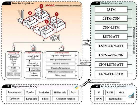
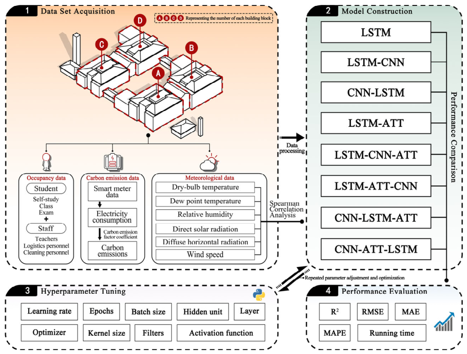
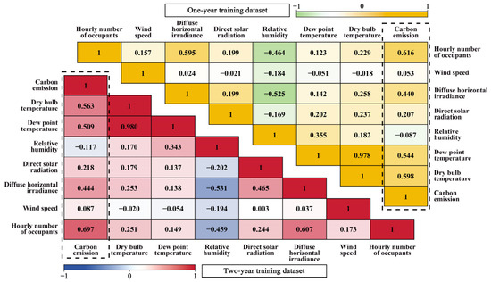
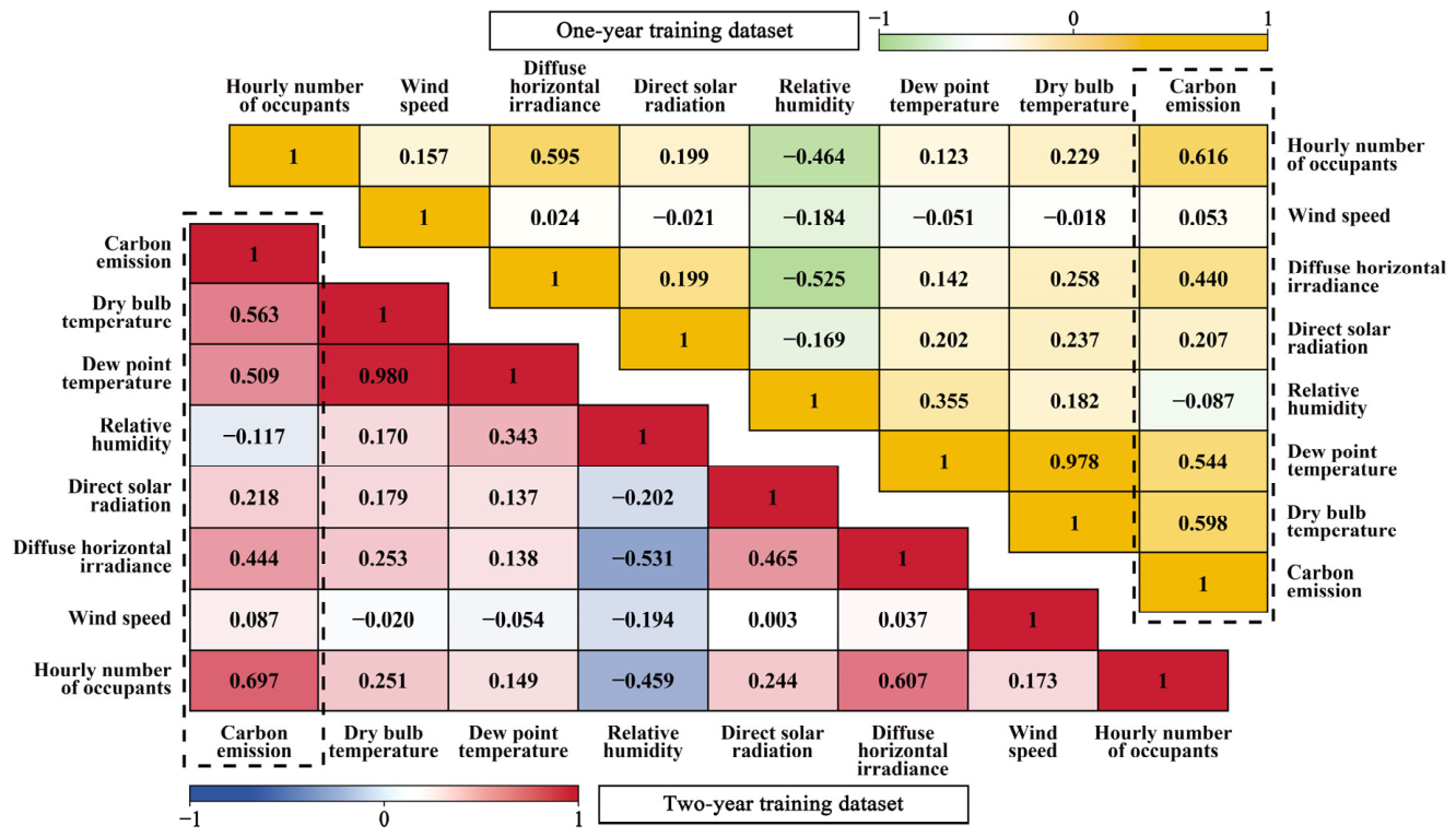
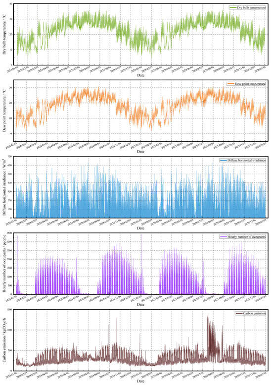
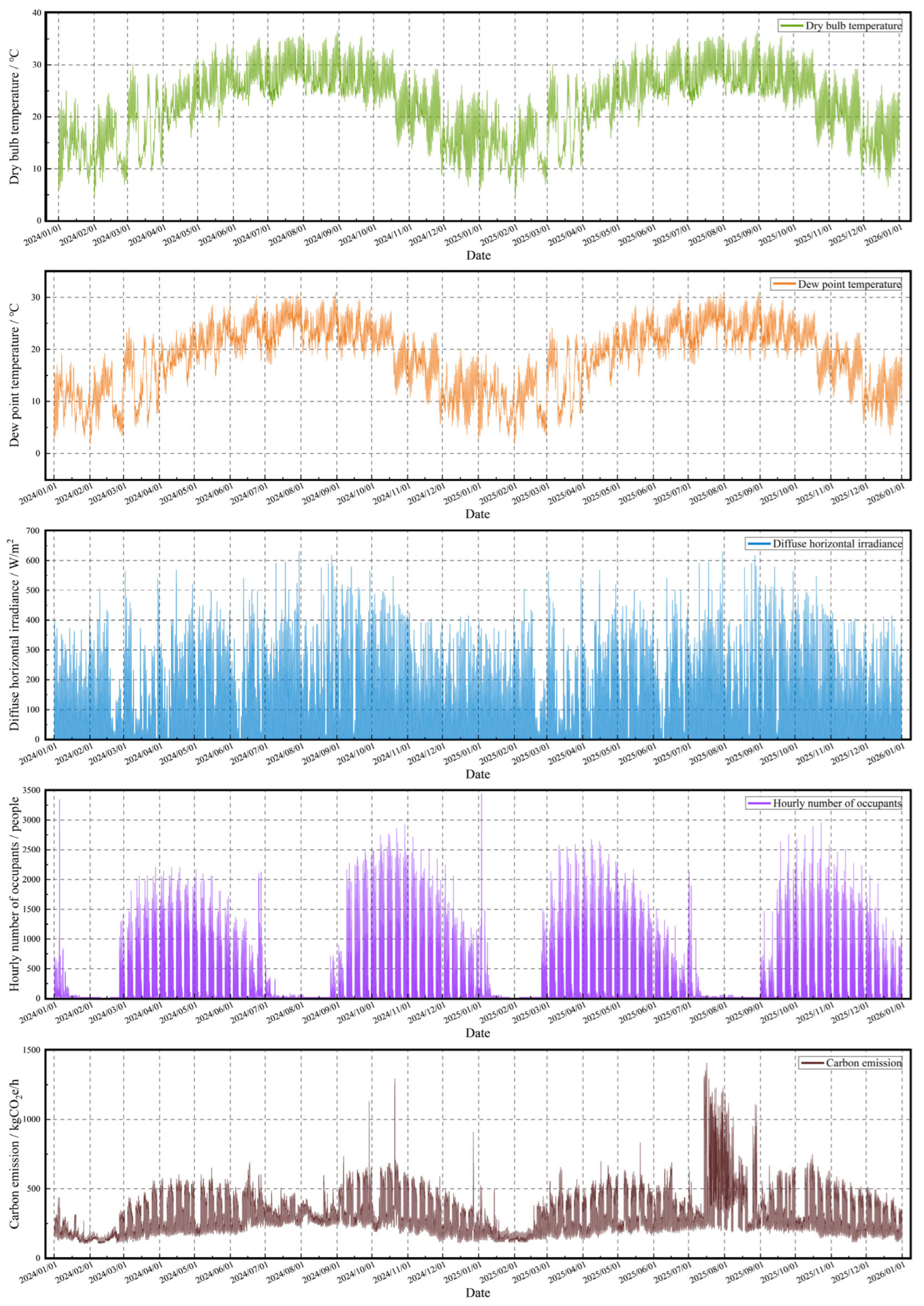
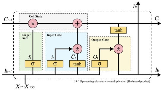
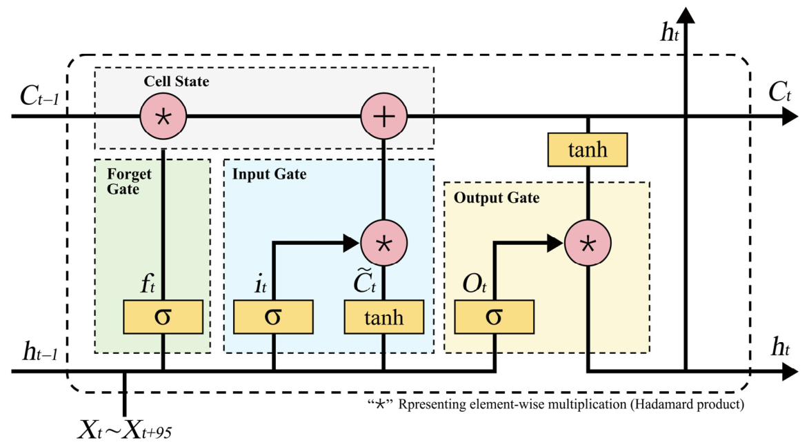
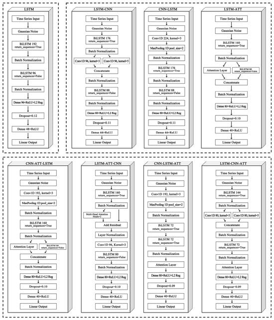
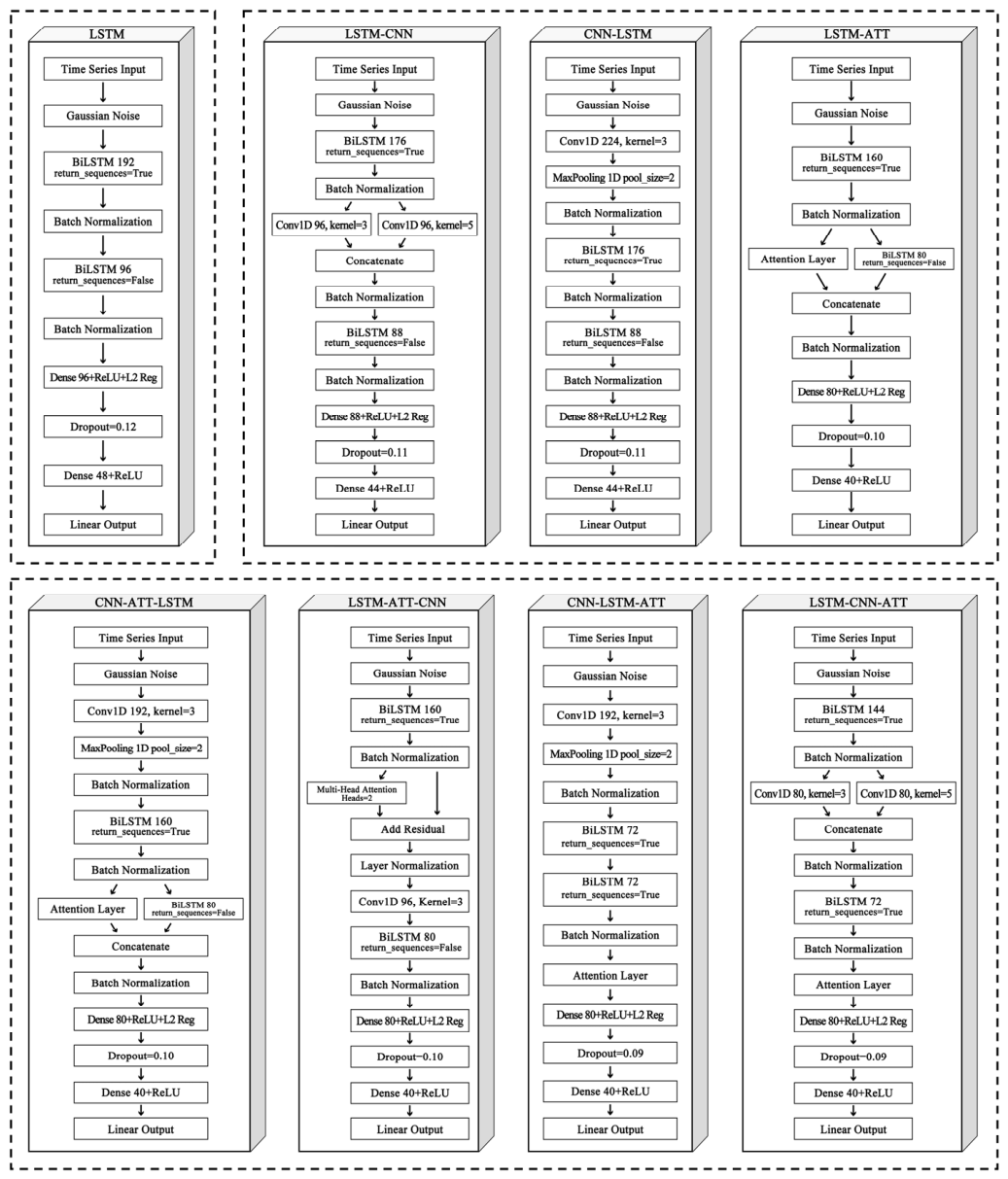
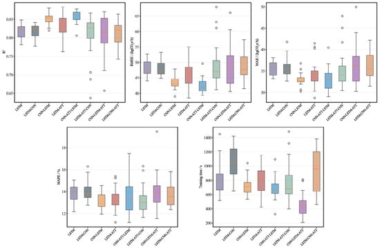
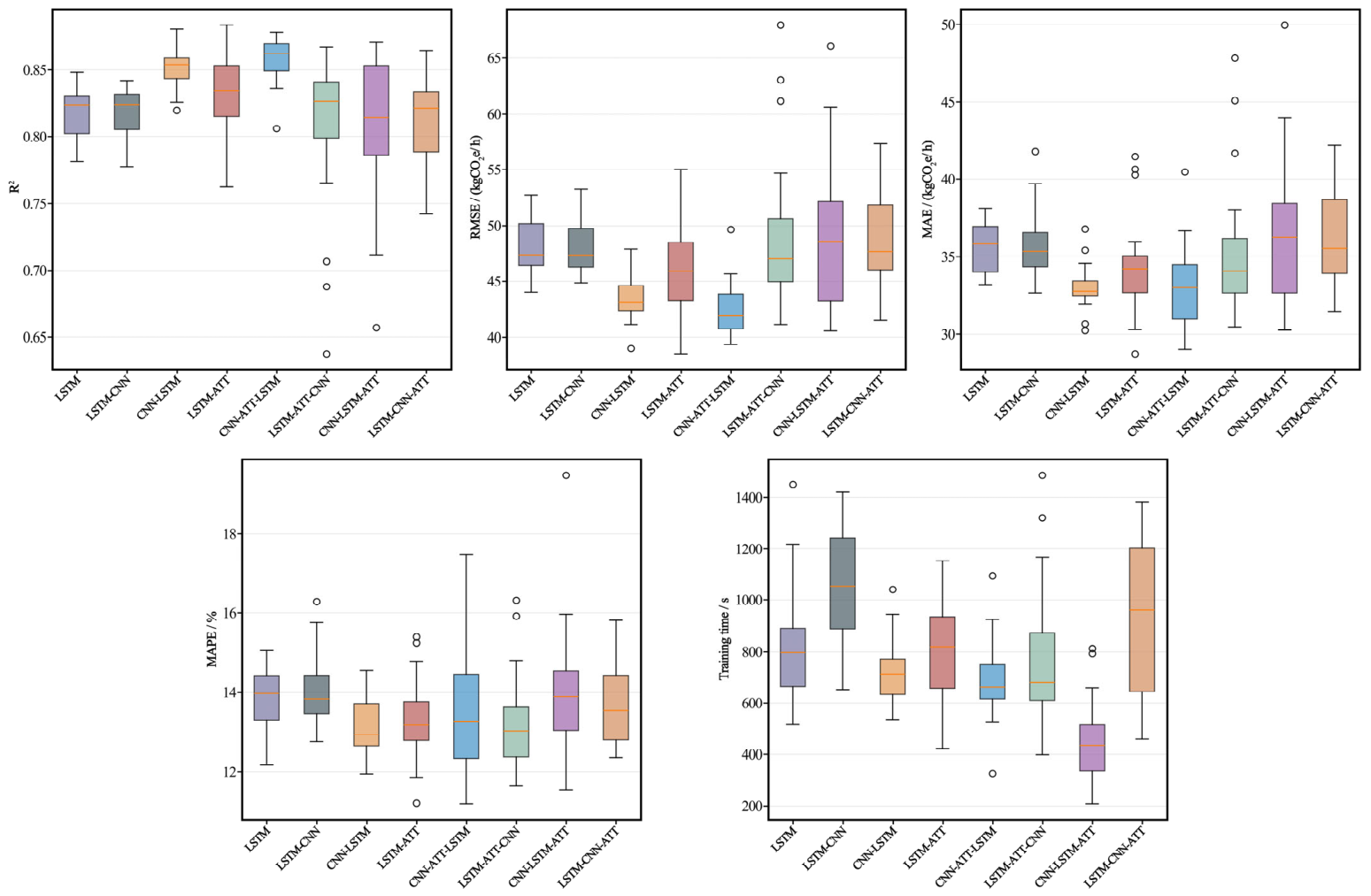
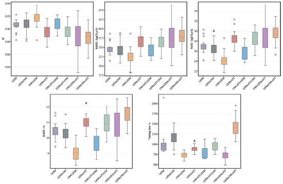
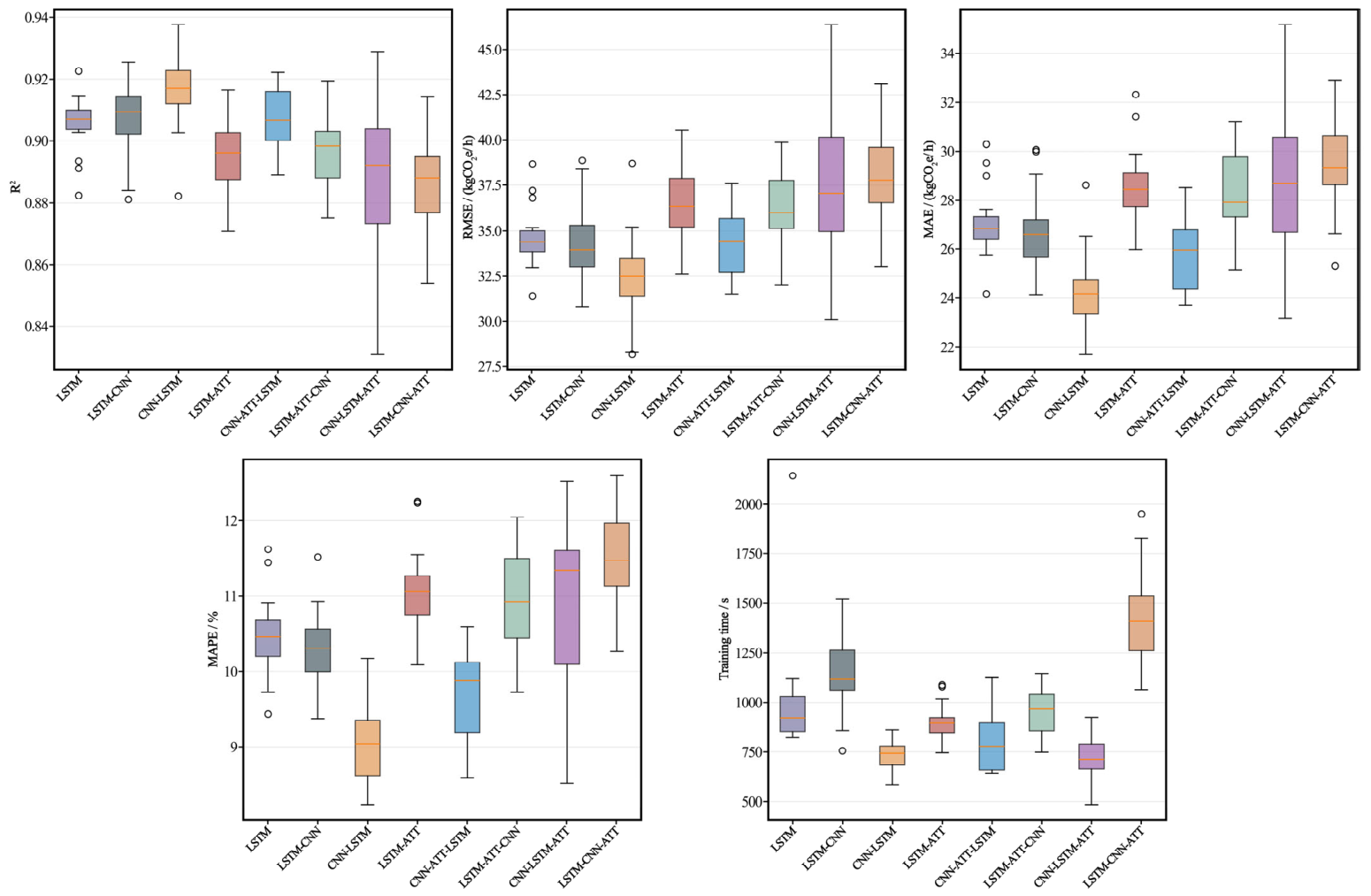
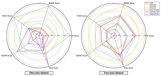
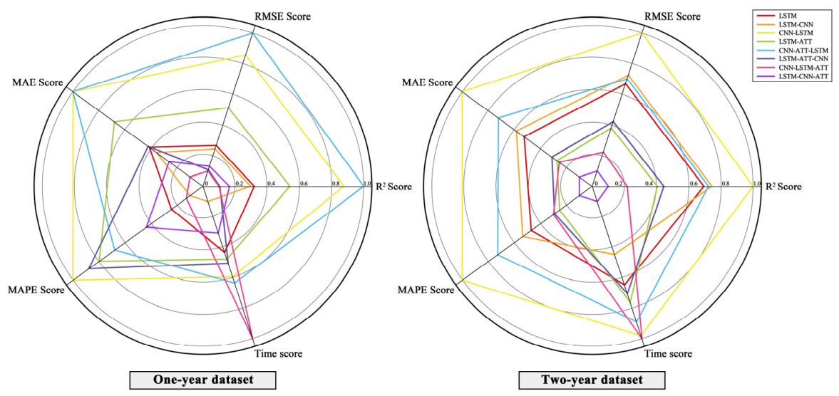
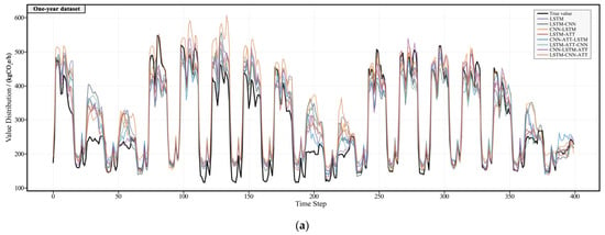
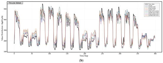
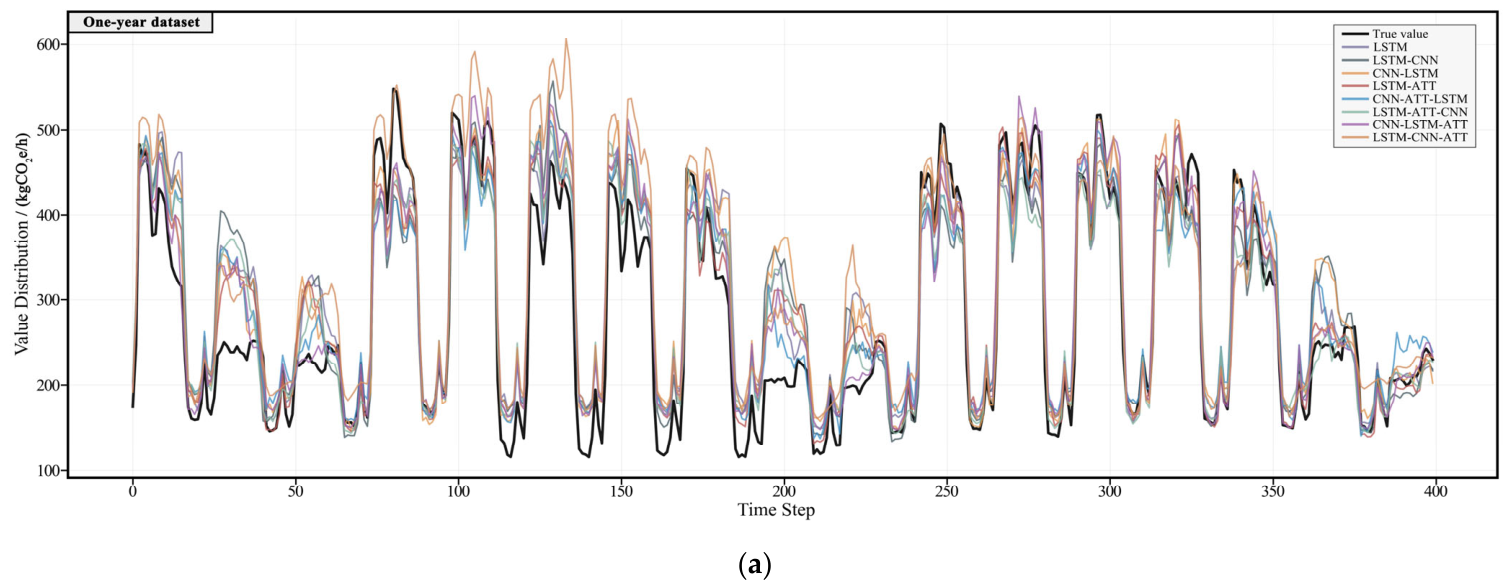
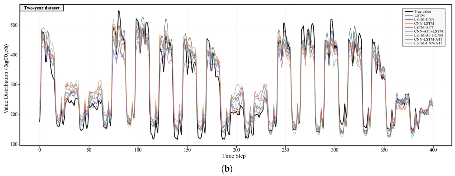
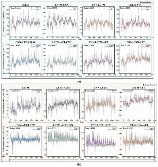
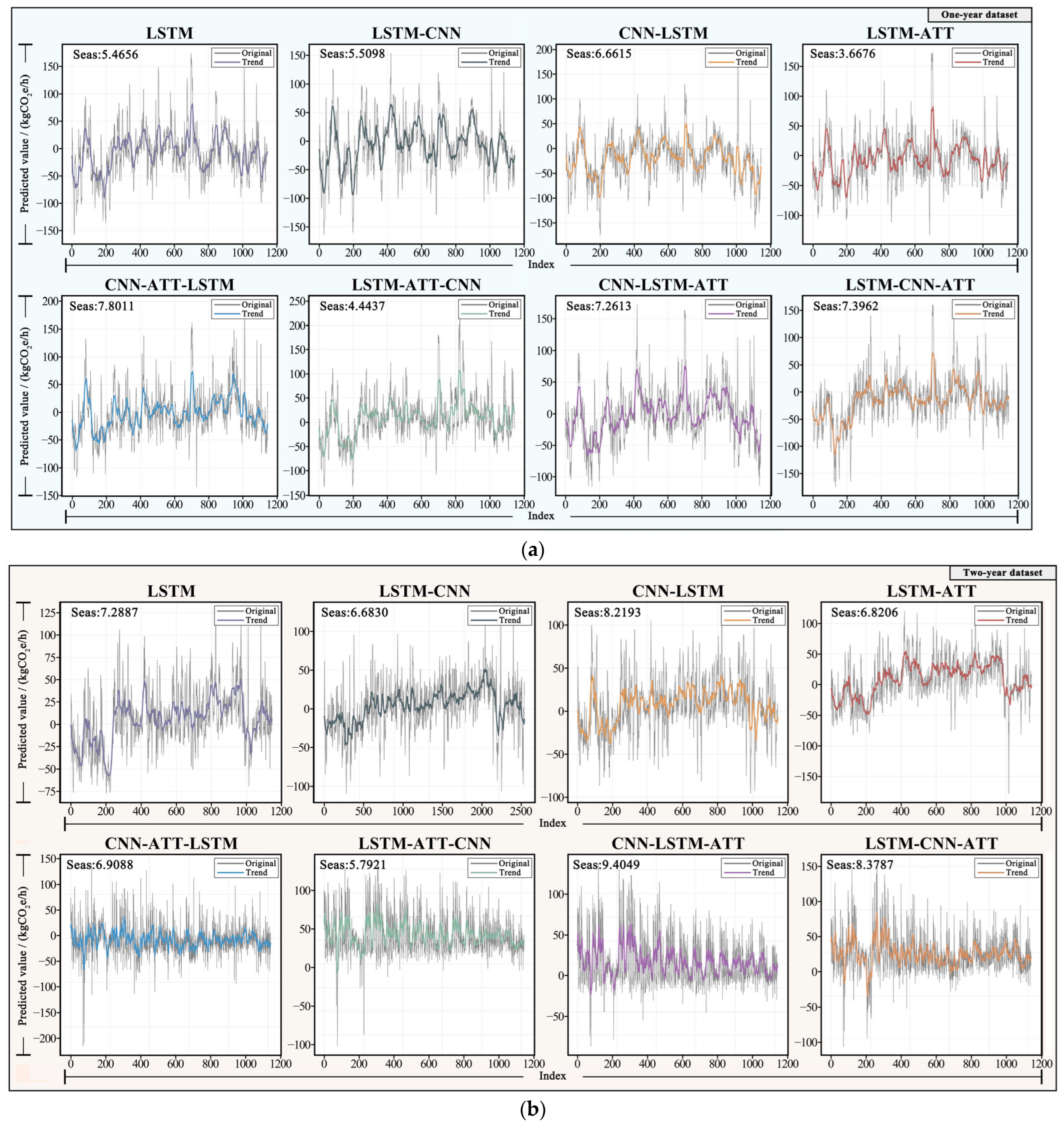
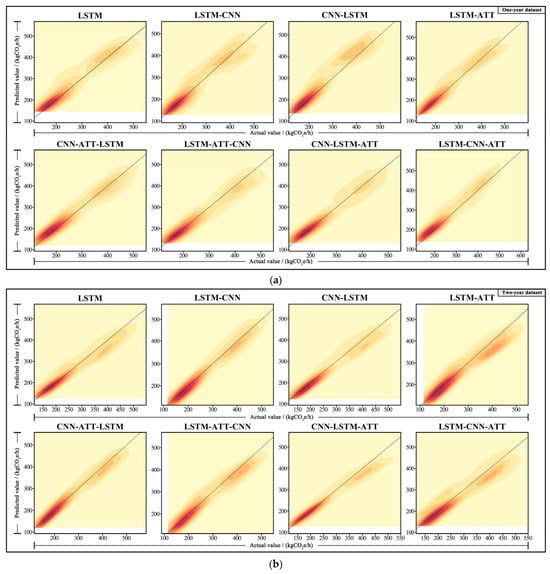
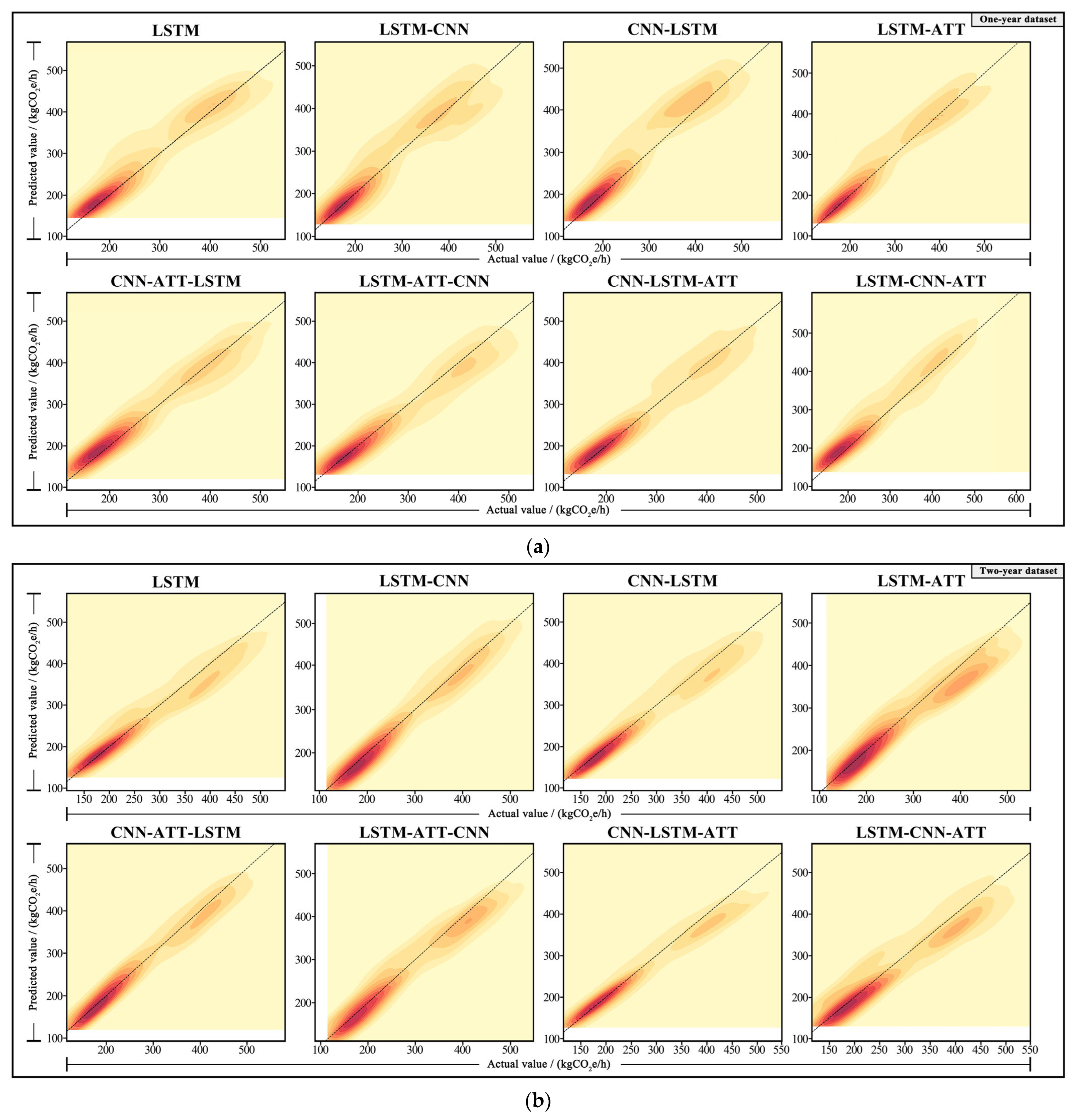

Disclaimer/Publisher’s Note: The statements, opinions and data contained in all publications are solely those of the individual author(s) and contributor(s) and not of MDPI and/or the editor(s). MDPI and/or the editor(s) disclaim responsibility for any injury to people or property resulting from any ideas, methods, instructions or products referred to in the content. |
© 2026 by the authors. Licensee MDPI, Basel, Switzerland. This article is an open access article distributed under the terms and conditions of the Creative Commons Attribution (CC BY) license.