Building-Level Multi-Scenario Seismic Damage Assessment of 1.49 Million Buildings in Ningxia: Building-Specific PGA Scaling and Spatial Association Analysis

Abstract

To characterize regional building-stock damage arising from the combined effects of spatially varying ground motions, building vulnerability, and exposure, this study develops a building-level, multi-scenario, and multi-record seismic damage assessment framework for 1,491,510 buildings across Ningxia, China. Frequent, design-basis, and rare earthquake scenarios were defined in accordance with China’s multi-level seismic design framework. Three sets of recorded ground motions, each comprising two orthogonal horizontal components, were individually scaled to the target peak ground acceleration (PGA) of each building and analyzed through nonlinear time-history analysis using the physics-based models implemented in YouSimulator. A total of 13,423,590 building–scenario–record results were obtained. Damage was characterized using building-count-averaged and floor-area-weighted damage indices (DIs), five damage grades, record-to-record sensitivity, and spatial autocorrelation at two grid resolutions. The building-count-averaged regional DIs were 0.063, 0.222, and 0.576 under the frequent, design-basis, and rare earthquake scenarios, respectively. The dominant damage state shifted from Grade 1 (essentially intact) to Grade 2 (slight damage) and then to Grade 4 (severe damage), indicating nonlinear transitions across damage thresholds. Under the rare earthquake scenario, 74.23% of the buildings reached Grades 4–5, and the three-record mean number of Grade 5 buildings was approximately 92,082. The floor-area-weighted DIs under the frequent and design-basis earthquakes were 1.68 and 1.31 times their building-count-averaged counterparts, respectively, indicating that floor-area weighting gives greater emphasis to buildings that contribute more exposed area. Approximately 844,627 rural detached houses reached Grades 4–5 and constituted the majority of buildings with severe damage. At the 0.025° grid scale, Moran’s I values were 0.429, 0.435, and 0.586 for the three scenarios, respectively (all p = 0.002), confirming significant spatial clustering. Although the regional mean DI under the rare earthquake scenario varied only from 0.563 to 0.598 among the three records, the proportion of buildings in Grades 4–5 ranged from 60.4% to 83.6%. Moreover, the Jaccard index between the top 10% of grids with high DI and those with high record sensitivity was only 0.039. These findings demonstrate that regional mean damage alone cannot adequately represent damage-grade composition, exposure, and record-to-record sensitivity within the selected record set. Damage severity, exposure scale, and record sensitivity should therefore be treated as complementary screening dimensions for regional retrofit prioritization, emergency resource allocation, and targeted verification. These screening dimensions and all statistics reported below are conditional on the present set of three-record pairs and on the specified scenario intensities.

1. Introduction

Earthquake consequences are not determined by ground-motion intensity alone, but arise from the combined effects of hazard, building vulnerability, and exposure. Classical probabilistic seismic hazard analysis established the relationship between ground-motion intensity and exceedance frequency [1]. Subsequent frameworks, including RISK-UE, HAZUS, and OpenQuake, incorporated building classification, vulnerability functions, and spatial exposure into regional seismic damage and loss assessment [2,3,4,5]. These approaches provide scalable frameworks for urban risk mapping, but their results are highly sensitive to the resolution of the building inventory, structural classification, site conditions, and the spatial scale of aggregation [6,7,8]. Vulnerability-function frameworks are computationally efficient and readily updated, but they characterize the average class behavior and cannot represent building-specific geometry, stiffness, or response; the physics-based building-level approach used here captures building-specific hazard input and response at the cost of much larger computational and parameter-data requirements.

Empirical damage matrices and analytical vulnerability curves are computationally efficient and readily applicable over large regions, but they generally use building classes rather than individual buildings as the basic unit of analysis. With advances in building-level data acquisition, parallel computing, and simplified nonlinear modeling, regional seismic damage simulation has begun to shift from statistical class mapping to building-level response analysis. Lu et al. [9] demonstrated parallel computing for refined urban models; Xiong et al. [10,11] developed nonlinear models and parameter-identification procedures for regional multistory and high-rise buildings; and Lu et al. [12] subsequently completed open-source nonlinear time-history and loss analyses for approximately 1.8 million buildings in the San Francisco Bay Area. Building-level methods preserve local variations in hazard and building attributes, but they retain building-specific attributes and input differences that class-based methods average out. Propagating uncertainty is not automatic; however, it must be explicitly embedded in the workflow [13,14]. In the present study, variability is examined through the scenario ladder and the three-record sensitivity analysis, whereas parameter uncertainty is not stochastically propagated.

YouSimulator is a building-stock seismic damage assessment platform designed for the nonlinear time-history analysis of urban building inventories. It automatically converts building inventories into simplified physics-based models and supports spatially nonuniform ground-motion input, damage calculation, and three-dimensional visualization. The platform has been applied to and validated against multiple earthquake cases [15,16,17,18]. Using this platform, Chen et al. [19] proposed a method for rapidly generating urban damage scenarios under nonuniform ground motions; Lin et al. [20] systematically examined detailed regional seismic damage assessment based on time-history dynamic analysis; Yuan et al. [16] combined high-resolution remote-sensing imagery with seismic simulation to rapidly assess the 2022 Luding M6.8 earthquake in Sichuan; and Chen et al. [18] further developed a dynamic assessment framework based on multisource data.

Ningxia lies in the tectonic transition between the northeastern margin of the Tibetan Plateau and the western margin of the Ordos Block. The Haiyuan Fault, Luoshan Fault, eastern Helanshan Fault, and fault systems within the Yinchuan Basin form a complex regional seismotectonic setting [21,22,23]. In this setting, building-level damage scenarios covering both urban and rural areas and multiple structural systems can estimate aggregate regional consequences while distinguishing highly vulnerable small subpopulations from highly exposed large populations. This study uses a region-wide building inventory for Ningxia to evaluate building-stock damage under frequent, design-basis, and rare earthquake scenarios defined by Chinese seismic design provisions. Building-specific hazard control, physical response, exposure statistics, record sensitivity, and spatial association are integrated into a single evidence chain. Results for all 1,491,510 buildings avoid the risk that sampling may mask small but highly vulnerable classes. Building-count and floor-area-weighted measures, continuous DIs, and five-grade compositions are reported together to distinguish high damage, high exposure, and high record sensitivity. Moran’s I at two spatial scales and the Jaccard index for top-decile grid sets are used to convert mapped patterns into testable statistical evidence.

2. Study Area and Building Inventory

2.1. Study Area and Seismotectonic Setting

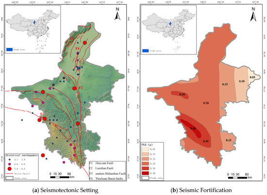
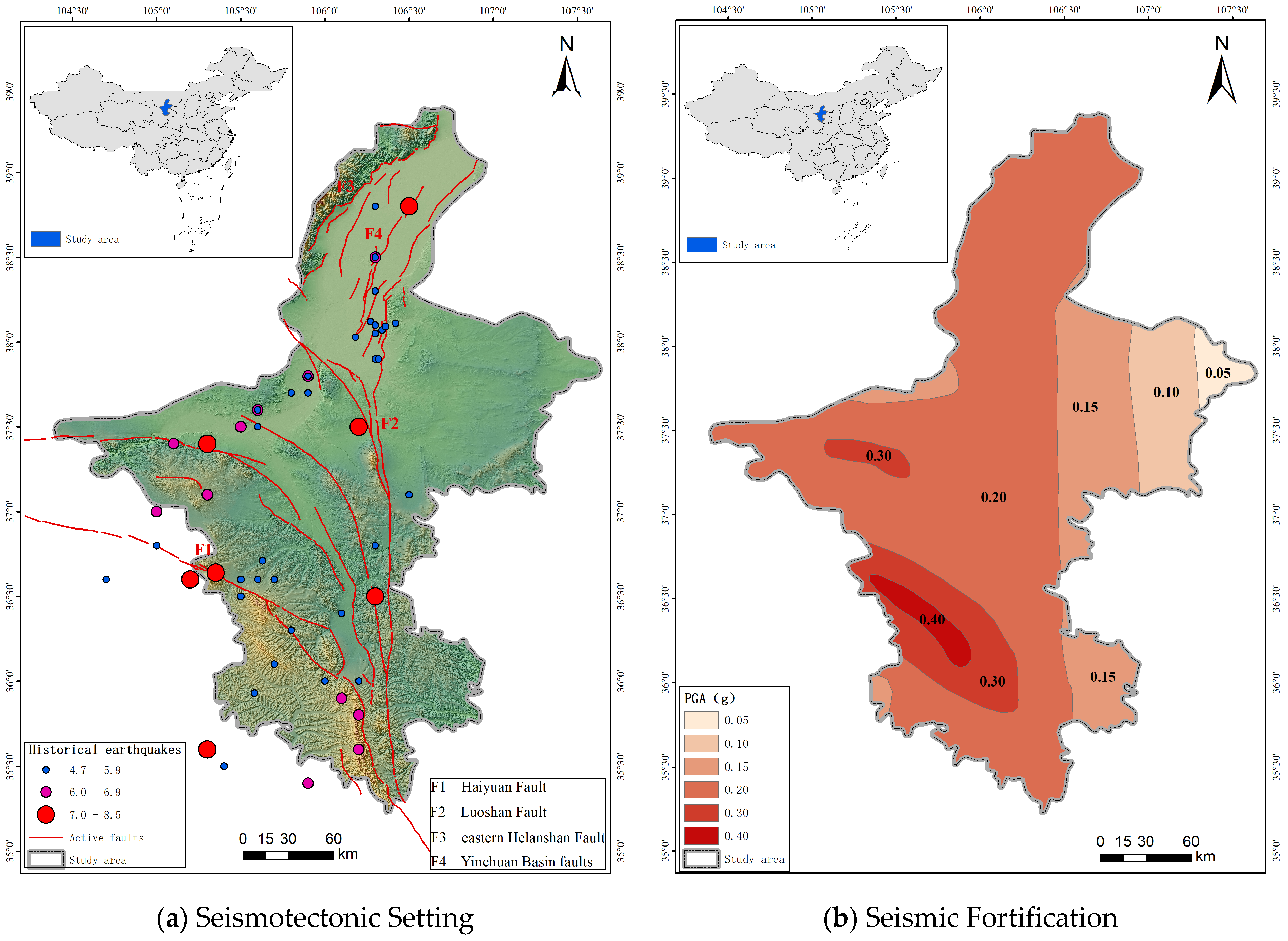
The study area covers the entire Ningxia Hui Autonomous Region, as Figure 1 presented. Southern Ningxia is affected by tectonic deformation along the northeastern margin of the Tibetan Plateau, where the Haiyuan Fault is characterized by major left-lateral strike-slip motion. In northern Ningxia, the Yinchuan Basin and the western margin of the Ordos Block contain the eastern Helanshan Fault, the Luoshan Fault, and intrabasin faults, as shown in Figure 1a. Geological and geomorphological studies show that different fault segments have distinct slip styles and activity rates, while a recent three-dimensional active-fault model further indicates contrasting tectonic assemblages and potential seismogenic structures between northern and southern Ningxia [21,22,23].

Figure 1. Study area: (a) seismotectonic setting, showing the major active fault systems of Ningxia (Haiyuan Fault, Luoshan Fault, eastern Helanshan Fault, and Yinchuan Basin faults) compiled from previous geological studies [21,22,23]; (b) seismic fortification level according to GB 18306-2015 [24], with the legend denoting the zoned design peak ground acceleration (PGA, in g) of each county-level unit (0.05 g to 0.40 g).

According to the national Seismic Ground Motion Parameters Zonation Map of China (GB 18306-2015) [24], as shown in Figure 1b, Ningxia is a region of relatively high seismic activity. It comprises five prefecture-level administrative divisions and is predominantly assigned a seismic fortification intensity of VIII. Yanchi County is assigned intensity VI, Pengyang County intensity VII, and most other counties, cities, and districts intensity VIII; Yinchuan is also designed for intensity VIII. The required seismic fortification level of a specific building additionally depends on its location, occupancy, structural system, and height. Important facilities such as schools and hospitals generally require enhanced seismic measures.

2.2. Building Inventory

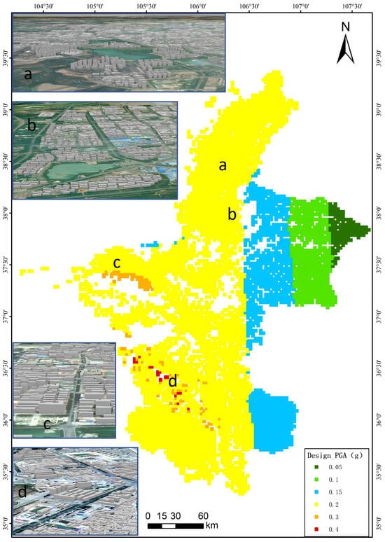
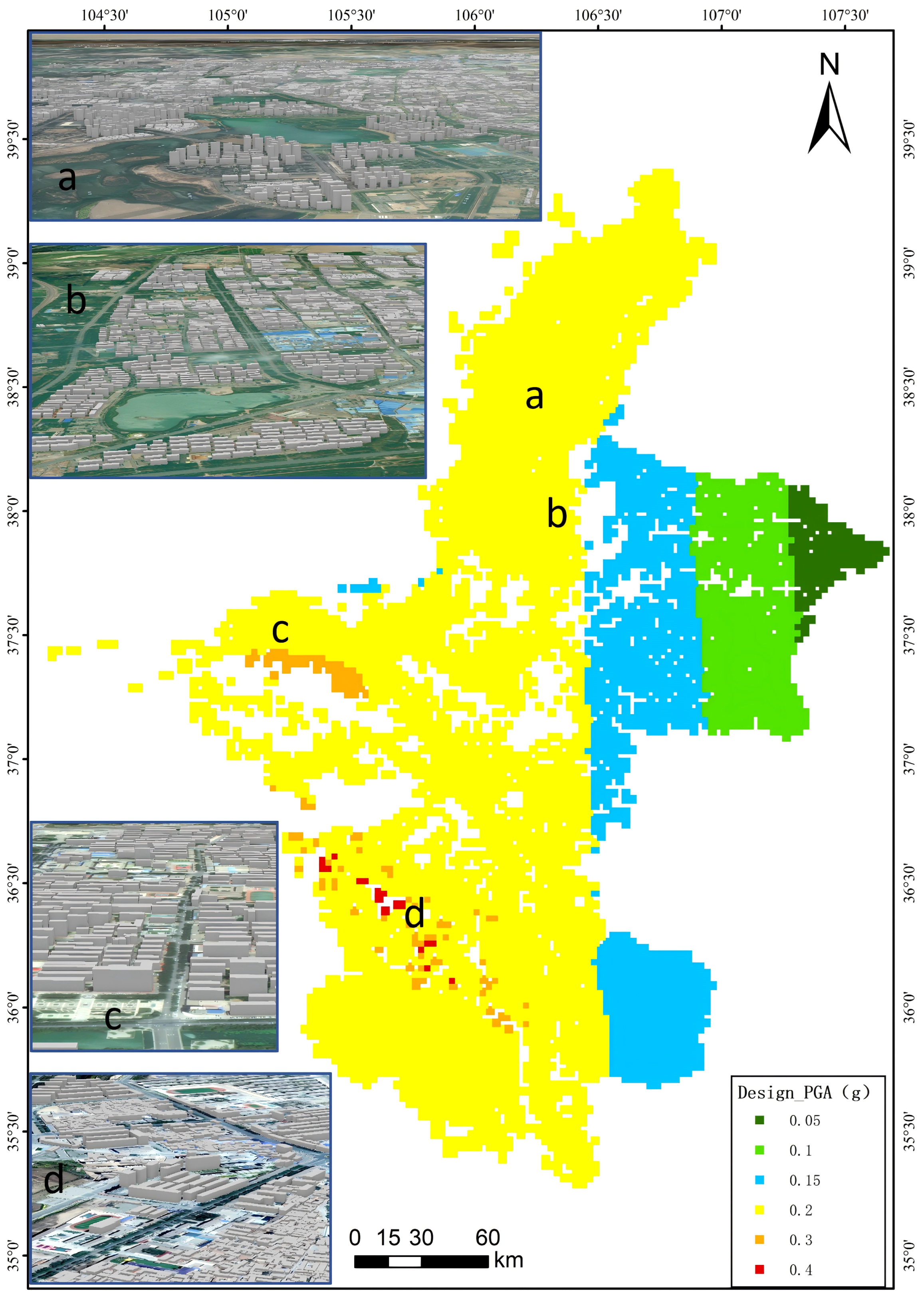
Figure 2 presents the building-specific design PGA for Ningxia on a 0.025° grid. The inventory contains 1,491,510 buildings with a total floor area of approximately 317.24 million m². Buildings are grouped by urban–rural setting and occupancy into five categories: urban non-residential, urban residential, rural detached residential, rural non-residential, and rural collective residential buildings (Table 1). Rural detached residential buildings number 1,054,924, accounting for 70.7% of all buildings but 37.6% of total floor area. Urban non-residential buildings account for only 9.9% by count but 31.3% by floor area. This asymmetry between building count and floor area requires damage results to be reported using both metrics. The inventory includes timber, steel, reinforced-concrete, strengthened-masonry, and non-engineered residential structures. Strengthened masonry comprises 1,276,891 buildings, representing 85.6% of the inventory and 58.6% of total floor area. Non-engineered residential buildings account for 6.4% by count but 20.2% by floor area. The larger floor-area share reflects a larger average per-building floor area of this category: the per-building floor areas of the inventory give 670.7 m² on average (median 239 m²; 75th percentile 708 m²) for non-engineered residential buildings, versus 145.5 m² on average (median 105 m²) for strengthened masonry; the class therefore contains a heavy tail of very large individual buildings, and the medians are the more robust class-level comparison. The area attribute combines the footprint and the story count of each building, and part of the tail may reflect aggregated multi-unit parcels in the source cadastre. In addition, 1,354,584 buildings are single story, corresponding to 90.8% of the inventory. The number of stories enters the response model directly through building height, mass, and the number of modeled degrees of freedom, and it covaries with the lateral force-resisting system: the stock is dominated by single-story masonry buildings, whereas the fewer mid-rise reinforced-concrete buildings have longer periods and different overstrength. Story group is therefore analyzed as a separate classification dimension (Section 4.2). Regional averages are therefore strongly governed by the stock of low-rise masonry buildings, whereas the relatively small numbers of steel and reinforced-concrete buildings may still contribute substantially to consequences because of their larger individual floor areas and functional importance. Building-classification systems such as GED4ALL emphasize that structural system, load-bearing material, number of stories, construction period, and occupancy should be encoded as separate dimensions rather than using a single occupancy label as a proxy for structural vulnerability [25].

Figure 2. Building-specific design PGA in CGCS2000 coordinates (0.025° grid).

Table 1. Inventory characteristics of the five building categories.

Project Category	Building Count	Share by Count	Floor Area (Million m2)	Share by Floor Area	Mean Number of Stories	Median Construction Year
Urban non-residential	146,937	9.9%	99.36	31.3%	1.70	2010
Urban residential	141,352	9.5%	45.89	14.5%	3.12	2007
Rural detached residential	1,054,924	70.7%	119.15	37.6%	1.01	1995
Rural non-residential	141,972	9.5%	50.51	15.9%	1.16	2005
Rural collective residential	6325	0.4%	2.33	0.7%	3.14	2015

3. Methodology

3.1. Earthquake Scenarios

Hazard inputs were divided into three seismic fortification scenarios—frequent, design-basis, and rare earthquakes—according to the seismic design level assigned to each building. For building i under scenario s, the target peak ground acceleration is denoted as PGA_target(i,s). GB 18306-2015 [24] specifies the zonation principles used to determine peak ground acceleration and characteristic response-spectrum periods for general construction projects in China, while GB 50011-2010 (2016 edition) [26] defines the multi-level seismic fortification framework for buildings. The frequent-earthquake scenario corresponds to an exceedance probability of approximately 63.2% in 50 years and a return period of approximately 50 years. The design-basis earthquake corresponds to an exceedance probability of approximately 10% in 50 years and a return period of approximately 475 years. The rare earthquake corresponds to an exceedance probability of approximately 2–3% in 50 years and a return period of approximately 1600–2500 years.

3.2. Ground-Motion Records and Building-Specific PGA Scaling

Three sets of recorded ground motions—El Centro 1940, Taft 1952, and RSN960 NORTHR LOS—were used, with two orthogonal horizontal components from each record input to YouSimulator. According to the PEER NGA-West2 database, El Centro 1940 is RSN 6 from the Imperial Valley-02 earthquake, recorded at El Centro Array #9 (Mw 6.95, R_JB = 6 km, Vs30 = 213.44 m/s; components I-ELC180/I-ELC270). Taft 1952 is RSN 15 from the Kern County earthquake, recorded at Taft Lincoln School (Mw 7.36, R_JB = 38 km, Vs30 = 385.43 m/s; components TAF021/TAF111). RSN960 NORTHR LOS is RSN 960 from the 1994 Northridge-01 earthquake, recorded at Canyon Country-W Lost Canyon (Mw 6.69, R_JB = 11 km, Vs30 = 325.60 m/s; components LOS000/LOS270) [27,28]. These three-record pairs were selected because they are well-documented reference motions widely used in regional time-history assessment and because they span different magnitudes (Mw 6.69–7.36), source-to-site distances (R_JB = 6–38 km), and site conditions (Vs30 = 213–385 m/s). The set therefore does not represent the full conditional distribution of potential ground motions in the region and is treated as an initial, demonstration set of inputs for scenario-based simulations.

A scale factor was then calculated from the target PGA of each building under scenario s. The same scale factor was applied to the X and Y components of each record to preserve their relative amplitudes. During preprocessing, each record pair was normalized following the baseline convention implemented in the program: the stored waveform of each record retains the amplitude ratio of its two horizontal components, and the peak of the governing (larger) component is at or near unity. PGA_ref(m) denotes the reference peak ground acceleration of record m after this normalization, i.e., the unscaled reference level to which the building-specific scale factor is applied, and the same reference value is used for both horizontal components.

For record m, the linear amplitude scale factor is defined as:

SF_i,s,m = PGA_target(i,s)/PGA_ref(m)

(1)

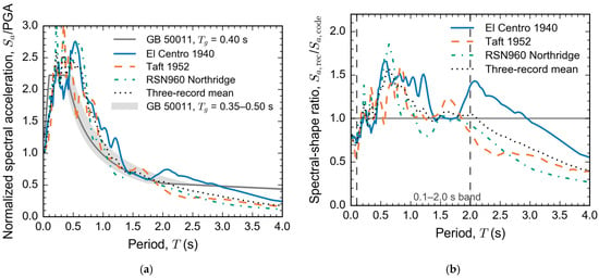
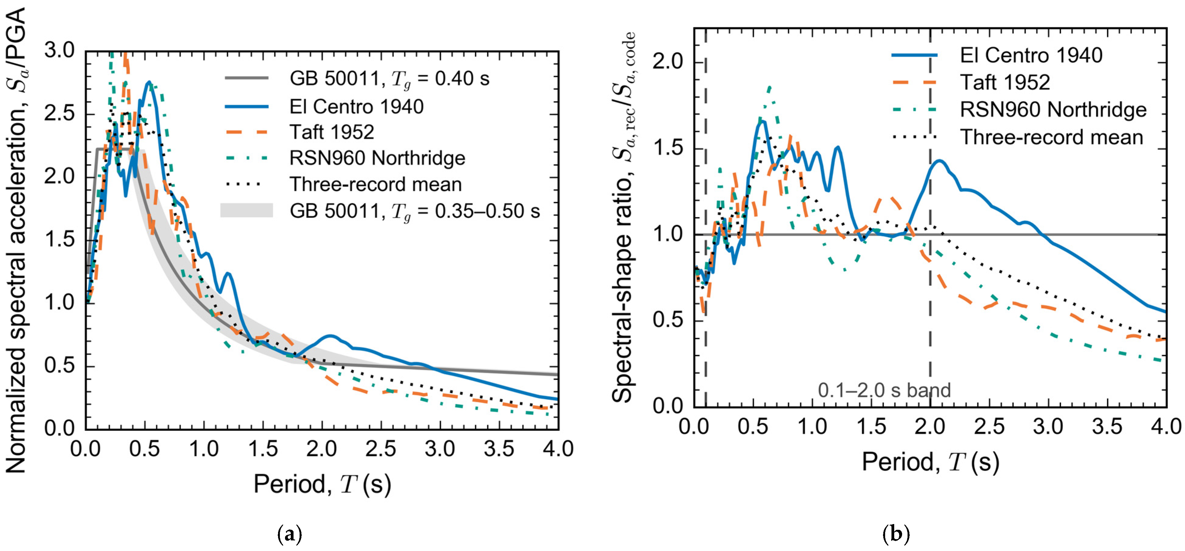
After scaling, the reference PGA of each of the three records equals PGA_target(i,s) for a given building and scenario. Differences in the response among records therefore mainly reflect spectral shape, duration, phase, and waveform characteristics other than PGA. Because the records are scaled in amplitude only, their spectral shapes are not matched to a Ningxia-specific target spectrum, and the spectral mismatch varies with the structural period. This mismatch is expected to affect most strongly the buildings whose fundamental periods fall in ranges where the scaled record spectra deviate most from the target shape, in particular four- to six-story buildings with higher-mode participation and buildings whose periods elongate as damage accumulates. The record-to-record differences reported below therefore combine spectral-shape, duration, and waveform effects and quantify sensitivity within this particular record set rather than the full ground-motion variability. Figure 3 compares the 5–damped, PGA-normalized response spectra of the three-record pairs (geometric mean of the two components of each pair) with the GB 50011-2010 (2016 edition) spectrum shape (representative Tg = 0.40 s; shaded range 0.35–0.50 s). In the illustrative 0.1–2.0 s band, the median ratio of the three-record-mean spectrum to the code shape is 1.08 (10th–90th percentile 0.99–1.40) and 86% of the period points exceed unity; the mismatch is not uniform across the band, being close to unity for periods below about 0.3 s, largest (median ratio about 1.1–1.4) between about 0.3 s and 1.0 s, and progressively falling below the code shape beyond about 2 s. Because most of the inventory is low-rise, the period range most relevant to strengthened masonry and non-engineered buildings is covered by the near-unity part of the band, whereas the 0.3–1.0 s excess is most relevant to mid-rise buildings, including the four- to six-story group.

Figure 3. Five-percent-damped normalized response spectra of the three ground-motion pairs after building-specific PGA scaling (geometric mean of the two orthogonal components of each pair), compared with the normalized GB 50011-2010 (2016 edition) spectrum shape for T_g = 0.40 s (shaded band: Tg = 0.35–0.50 s). (a) Normalized spectra and code range; (b) record-to-code ratio. The comparison is a spectral-shape screening: site class, building-specific T_g, and structural periods differ across the inventory, and code compliance cannot be decided from this figure alone.

3.3. Seismic Response Analysis of Buildings

YouSimulator employs a simplified physics-based modeling and nonlinear time-history analysis framework developed for urban building stocks. Automated modeling algorithms use building geometry and attribute data to generate simulation models and perform elastic-plastic time-history analyses for damage estimation. Each building is represented by a multiple-degree-of-freedom, multi-shear-spring model that accounts for the coupled effects of bidirectional horizontal ground motion [29]. The story-level restoring-force backbone curve is defined by the yield point, peak-capacity point, and collapse point, with hysteretic behavior incorporating stiffness degradation, strength degradation, and pinching. Seismic damage is determined from the maximum interstory drift and the corresponding damage index [20]. The backbone-curve parameters of each story spring are derived from the inventory attributes (structural type, construction period, number of stories, and story geometry) through the automated parameter-assignment rules of the platform, which follow the parameter-determination procedures of [10,11,20]. The story strength is set as a fixed fraction of the elastic shear force associated with the rare-earthquake level of the Chinese code at the building location, scaled by the type factors of Table 2, and the drift capacities follow the same type-factor scheme; the trilinear backbone is completed by post-yield and post-peak stiffness ratios, a peak-to-yield strength ratio of 1.5–1.6, a residual strength of 80% of the peak at collapse, and small random strength and deformation factors. Hysteretic behavior follows the bilinear elastoplastic and degrading options of the multi-shear-spring model [29].

Table 2. Definitions of seismic damage grades.

Damage Grade	Damage Index (DI)	Definition
1	$\mathit{DI}=0.10\times {\displaystyle \frac{d}{d_y}}$ 0 ≤ d ≤ dy	All components are intact, or only minor damage occurs in some nonstructural components. The building may remain in use without repair.
2	DI = 0.10 + 0.20 × (d − dy)/(Δ/6) dy < d ≤ dy + Δ/6	Visible cracks occur in some components. The building may remain in use without repair or after minor repair.
3	DI = 0.30 + 0.25 × (d − dy − Δ/6)/(Δ/3) dy + Δ/6 < d ≤ dy + Δ/2	Most structural components exhibit minor cracking, and a few exhibit evident cracking. Some nonstructural components are severely damaged. The building may remain in use after general repair.
4	DI = 0.55 + 0.30 × (d − dy − Δ/2)/(Δ/2) dy + Δ/2 < d ≤ du	Most structural components are severely damaged, and some nonstructural components have partially collapsed. Repair is difficult.
5	DI = 0.85 + 0.15 × (d − du)/d d > du	The building is near collapse or has collapsed and is not repairable.

Note: d is the maximum interstory drift ratio over all stories and over the entire time history; this definition is consistent with the archived per-story result records, in which each story’s damage index accumulates the maximum deformation over the entire time history. d_y and d_u are the nominal yield and nominal collapse interstory drifts of the controlling story; Δ = d_u − d_y; and all quantities are dimensionless drift ratios, consistent with the archived model files. A DI exactly equal to a grade boundary belongs to the upper grade, i.e., the destroyed grade begins at DI = 0.85.

3.4. Damage Indices and Grades

With reference to the Chinese Seismic Intensity Scale (GB/T 17742-2020) [30], simulated building damage is classified into five grades: essentially intact, slight damage, moderate damage, severe damage, and destroyed. To account for the characteristics and performance limits of each structural type, the damage state is determined from the relationship between the maximum interstory drift response and the corresponding story-level nominal yield and collapse drifts, as defined in Table 2. The DI boundaries between adjacent grades are 0.10, 0.30, 0.55, and 0.85. The nominal yield drift is the interstory deformation separating the essentially intact and damaged states; for structures without a distinct yield point, it is determined using the equal-energy principle. The nominal collapse drift is the interstory deformation separating severe damage from destruction or collapse and also represents the boundary between repairable and irreparable response. It is taken as the interstory deformation corresponding to a post-peak strength reduction to 80% of the peak strength. Regional damage is evaluated using a floor-area-weighted mean of the building DIs.

3.5. Ground-Motion Record Sensitivity, Classification, and Spatial Statistics

The record sensitivity of building i under scenario s is defined as the range of the DI across the three records, R_i,s = max_m(DI_i,s,m) − min_m(DI_i,s,m). Whether the records assign different damage grades to the same building is also recorded. Because M = 3, the DI range and damage-grade instability rate are used only to describe sensitivity within the present record set; confidence intervals and quantile estimates are not constructed. The range is preferred here over the standard deviation or coefficient of variation because, with only three records, it is directly interpretable as the worst-to-best spread within the selected set and requires no distributional assumption; it is, however, strongly dependent on the number of records and cannot estimate the dispersion of any larger population. Classification analyses group buildings by project category, structural type, story group, construction period, and design PGA from the source shapefile. For each factor, a one-way marginal η² is calculated as the ratio of between-group sum of squares to total sum of squares. Because the factors are strongly correlated, the η² values represent only the descriptive explanatory power of each classification; They cannot be added or interpreted as independent causal effects. These correlations arise because structural type is jointly determined with story height, occupancy, construction period, and location, so each single-factor η² also absorbs the variation shared with the other factors; the story-by-structure cross-tabulation and the PGA-by-structure stratification (Section 4.3) are provided to make the compositional overlaps explicit. PGA and structural type are also treated as a joint stratification to examine how well the combination of hazard and structural vulnerability describes variations in the DI.

Spatial analysis uses building-footprint centroids. DI is first averaged with equal weight across the three records and then aggregated to a 0.025° regular grid. A cell is included in correlation and hotspot-set analyses only if it contains at least 10 buildings. Global Moran’s I is calculated using rook-contiguity weights, and spatial autocorrelation is tested using 499 random permutations; the p-value is calculated as (number of equally or more extreme permutations + 1)/(499 + 1). A cell enters these analyses only if it contains at least 10 buildings; among the 5173 qualifying cells, 62 isolated cells have no rook neighbor inside the study area and are retained with zero contiguity weight, the standard behavior of rook weights near an irregular boundary; a sensitivity check that excludes these cells is reported in Section 4.3. To evaluate the scale effects associated with the modifiable areal unit problem (MAUP), adjacent 2×2 cells are aggregated to 0.05° and the analysis is repeated. Spearman rank correlation is used to quantify monotonic associations between DI and PGA, building count, floor area, and record-to-record DI range. The Jaccard index, J = |A∩B|/|A∪B|, measures the overlap between the top 10% grid sets, while the Gini coefficient, obtained by ordering cells by their Grade 4–5 count and integrating the resulting Lorenz curve, describes the concentration of Grade 4–5 building counts across all populated grid cells (6404 cells, including cells with zero Grade 4–5 buildings). The Gini coefficient is reported as a descriptive concentration measure and is complemented by the number of non-zero cells and the largest-cell share reported in Section 4.3. High DI, high exposure, and a large record range respectively indicate consequence severity, the potential scale of intervention, and the need for priority verification; no single ranking can substitute for the others [31,32]. Because the 10% top-decile threshold is a convention, the overlap analysis was repeated at the 5% and 20% thresholds under the rare earthquake at the 0.025° grid (Table 3); the limited overlap between the high-DI and high-record-range sets persists across these thresholds.

Table 3. Sensitivity of the overlap analysis to the top-set threshold (rare earthquake scenario, 0.025° grid; 5173 qualifying cells). Top-set sizes are 259, 518, and 1035 cells at the three thresholds.

Top-Set Threshold	J (High DI, High Record Range)	J (High DI, High Floor Area)
Top 5%	0.026	0.028
Top 10%	0.039	0.057
Top 20%	0.059	0.116

4. Results

4.1. Building-Stock Damage Under Different Earthquake Scenarios

The Ningxia building stock is dominated by rural detached residential buildings and strengthened masonry. Rural detached residential buildings account for 70.7% of the inventory by count but 37.6% by floor area, whereas urban non-residential buildings account for 9.9% by count but 31.3% by floor area. Structurally, strengthened masonry represents 85.6% of all buildings. Non-engineered residential buildings comprise only 6.4% by count but 20.2% by floor area. Consequently, the same regional mean DI may be driven simultaneously by a large number of small buildings and a small number of large buildings, making it necessary to distinguish between building-count and floor-area metrics.

The building-count-averaged regional DI increased from 0.063 under the frequent earthquake to 0.222 under the design-basis earthquake and 0.576 under the rare earthquake, corresponding to increases by factors of 3.52 and 2.60 between successive scenarios. Figure 4 shows the stepwise increase in the regional mean and its record-to-record range, whereas Figure 5 shows the accompanying redistribution across the five damage grades. The dominant damage grades under the frequent, design-basis, and rare earthquake scenarios were Grade 1 (essentially intact; 90.0%), Grade 2 (slight damage; 91.3%), and Grade 4 (severe damage; 68.1%), respectively. Increasing scenario intensity therefore did not simply shift the DI of every building by a constant amount; instead, the regional distribution concentrated first in Grade 2 and subsequently in Grade 4.

Figure 4. Regional mean damage index and the range across the three records for each earthquake scenario. Points denote the three-record mean of the regional mean DI, and vertical lines span the minimum-to-maximum range of the record-specific regional means.

Figure 4. Regional mean damage index and the range across the three records for each earthquake scenario. Points denote the three-record mean of the regional mean DI, and vertical lines span the minimum-to-maximum range of the record-specific regional means.

Figure 5. Five-grade damage composition under the three earthquake scenarios. Percentages are shares of the building count in each grade, and the corresponding mean building counts are listed in Table 4.

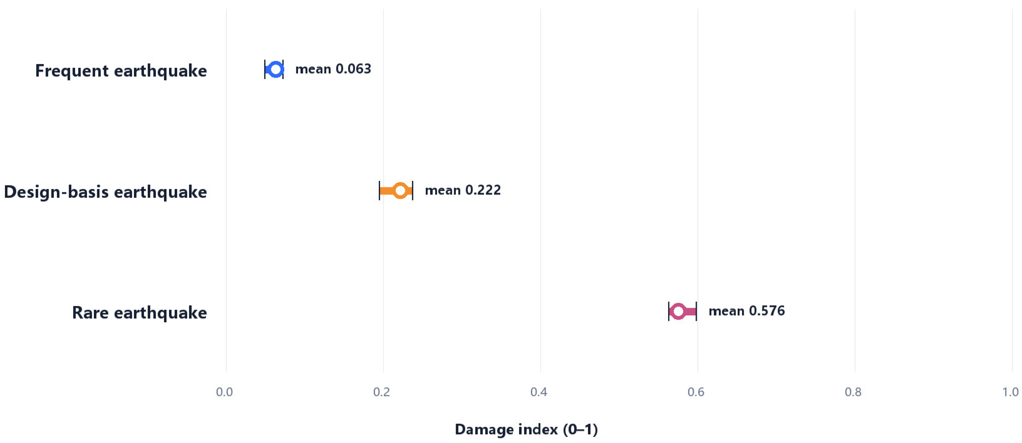
Figure 5. Five-grade damage composition under the three earthquake scenarios. Percentages are shares of the building count in each grade, and the corresponding mean building counts are listed in Table 4.

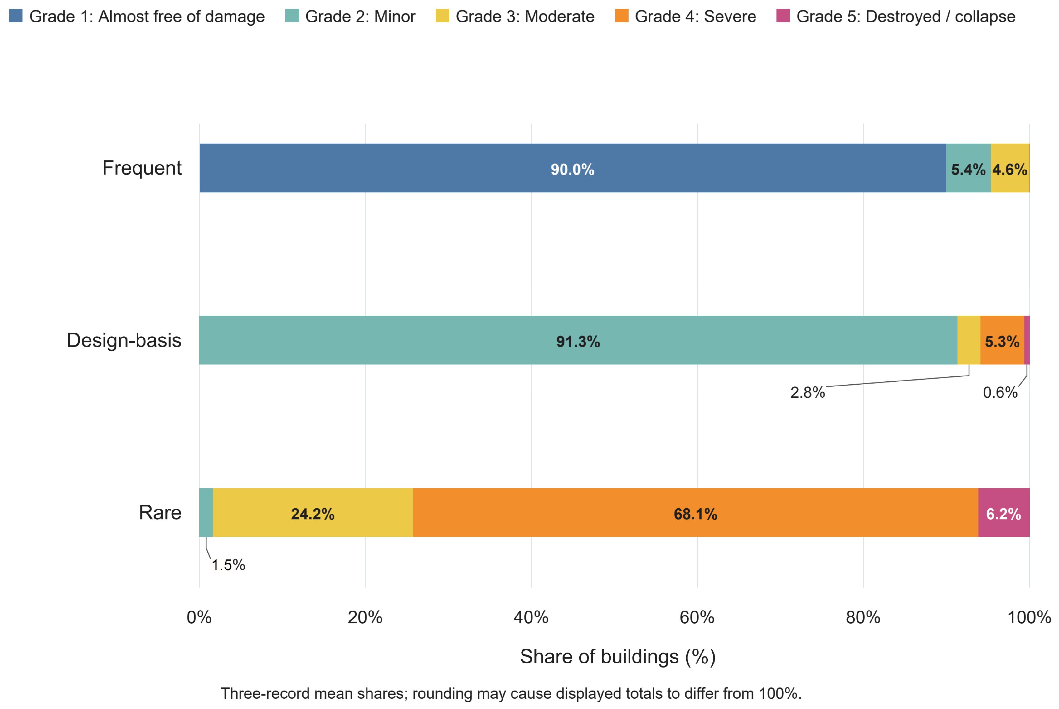
Table 4. Mean building counts by damage grade under the three earthquake scenarios (means of the per-record counts over the three records).

Scenario	Grade 1	Grade 2	Grade 3	Grade 4	Grade 5
Frequent	1,342,094	80,209	68,844	362	0
Design-basis	29	1,362,093	41,538	78,336	9514
Rare	3	23,678	360,686	1,015,061	92,082

Table 4. Mean building counts by damage grade under the three earthquake scenarios (means of the per-record counts over the three records).

Scenario	Grade 1	Grade 2	Grade 3	Grade 4	Grade 5
Frequent	1,342,094	80,209	68,844	362	0
Design-basis	29	1,362,093	41,538	78,336	9514
Rare	3	23,678	360,686	1,015,061	92,082

The floor-area-weighted DIs under the frequent and design-basis earthquakes were 0.106 and 0.290, respectively, corresponding to 1.68 and 1.31 times the building-count means. The two measures were similar under the rare earthquake. This convergence indicates that damage to large buildings is relatively prominent under the lower-intensity scenarios. As the scenario intensity increases, large numbers of low-rise masonry buildings enter the high-damage range, causing the building-count and floor-area regional means to converge. The higher area-weighted values indicate that the estimated damage field assigns greater weight to buildings contributing more floor area; the difference reflects the joint distribution of floor area with structural type, occupancy, and construction period, and should not be read as evidence that larger buildings are intrinsically more vulnerable or that the building-count mean is statistically biased.

Under the rare earthquake, the corresponding three-record mean increased to approximately 92,082 buildings, or 6.17% of the inventory. These buildings represented 61.85 million m², or 19.49% of the total floor area. The floor-area share exceeded the building-count share, indicating that the destroyed or collapsed grade contains a disproportionate number of larger buildings. Under the design-basis earthquake, the mean number of Grade 5 buildings across the three records was approximately 9514.

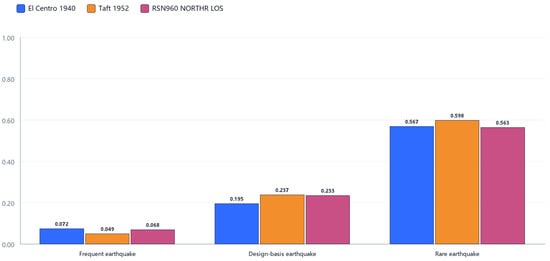
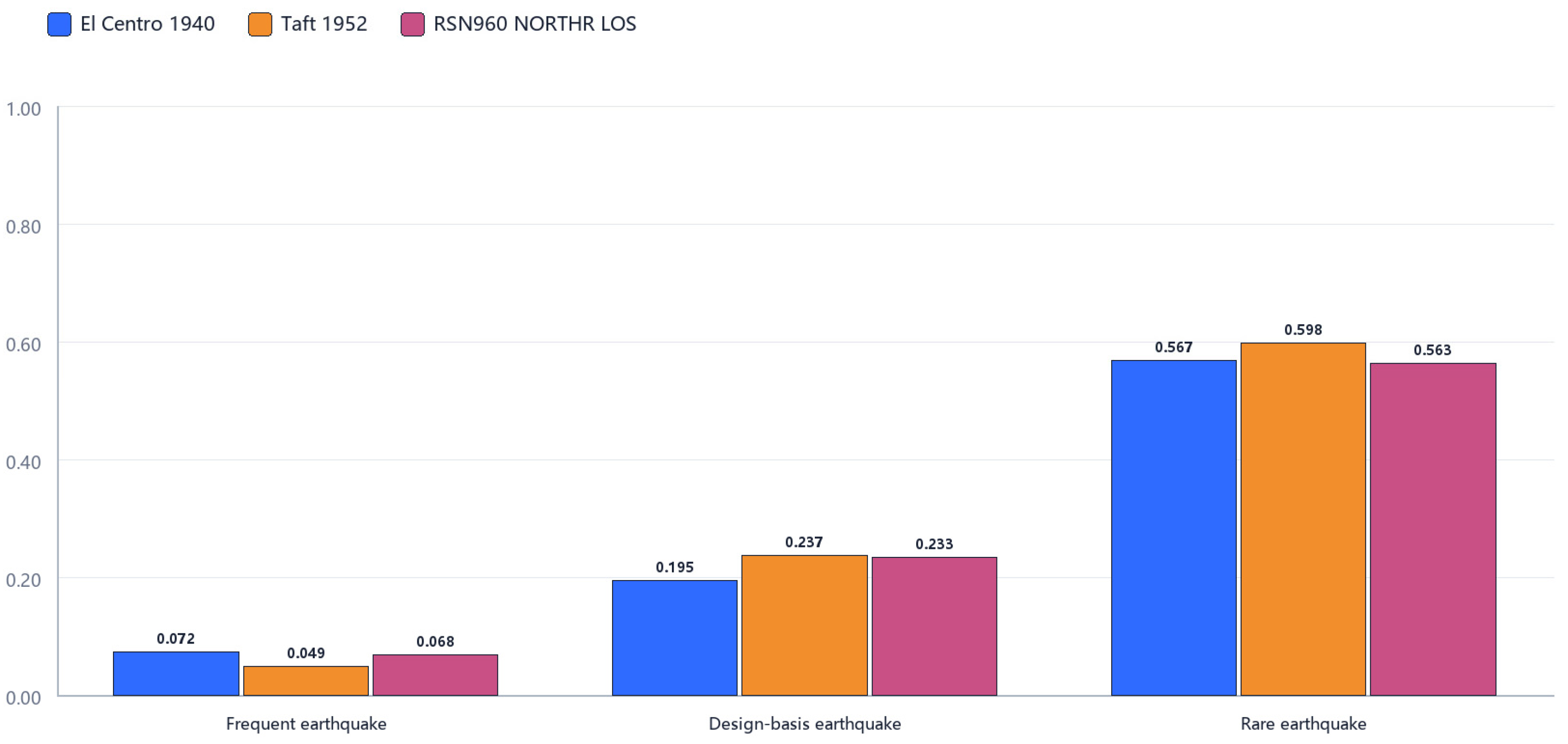
Figure 6 compares the three ground-motion records on a common basis after building-specific PGA scaling. Across the three records, the regional mean DI ranged from 0.049 to 0.072 under the frequent earthquake, from 0.195 to 0.237 under the design-basis earthquake, and from 0.563 to 0.598 under the rare earthquake. The corresponding coefficients of variation among record-specific means decreased from 0.160 to 0.086 and 0.027. The relatively high variation under the frequent earthquake partly reflects the near-zero mean, whereas convergence of the mean under the rare earthquake may result from the large number of buildings entering the high-damage range.

Figure 6. Regional mean damage index for the three ground-motion records after building-specific PGA scaling.

Nevertheless, under the rare earthquake the proportion of Grade 4–5 buildings ranged from 60.4% to 83.6% across the three records, far exceeding the relative variation in the mean DI; the Grade 5 proportion ranged from 6.1% to 6.4%. This finding shows that a mean DI can compress important distributional differences: two records can produce similar regional means while assigning large numbers of buildings to different damage grades. For retrofit decisions, damage-grade composition and tail proportions are more sensitive than a single mean value.

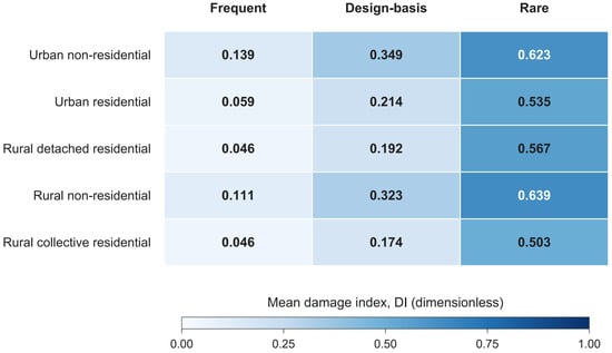
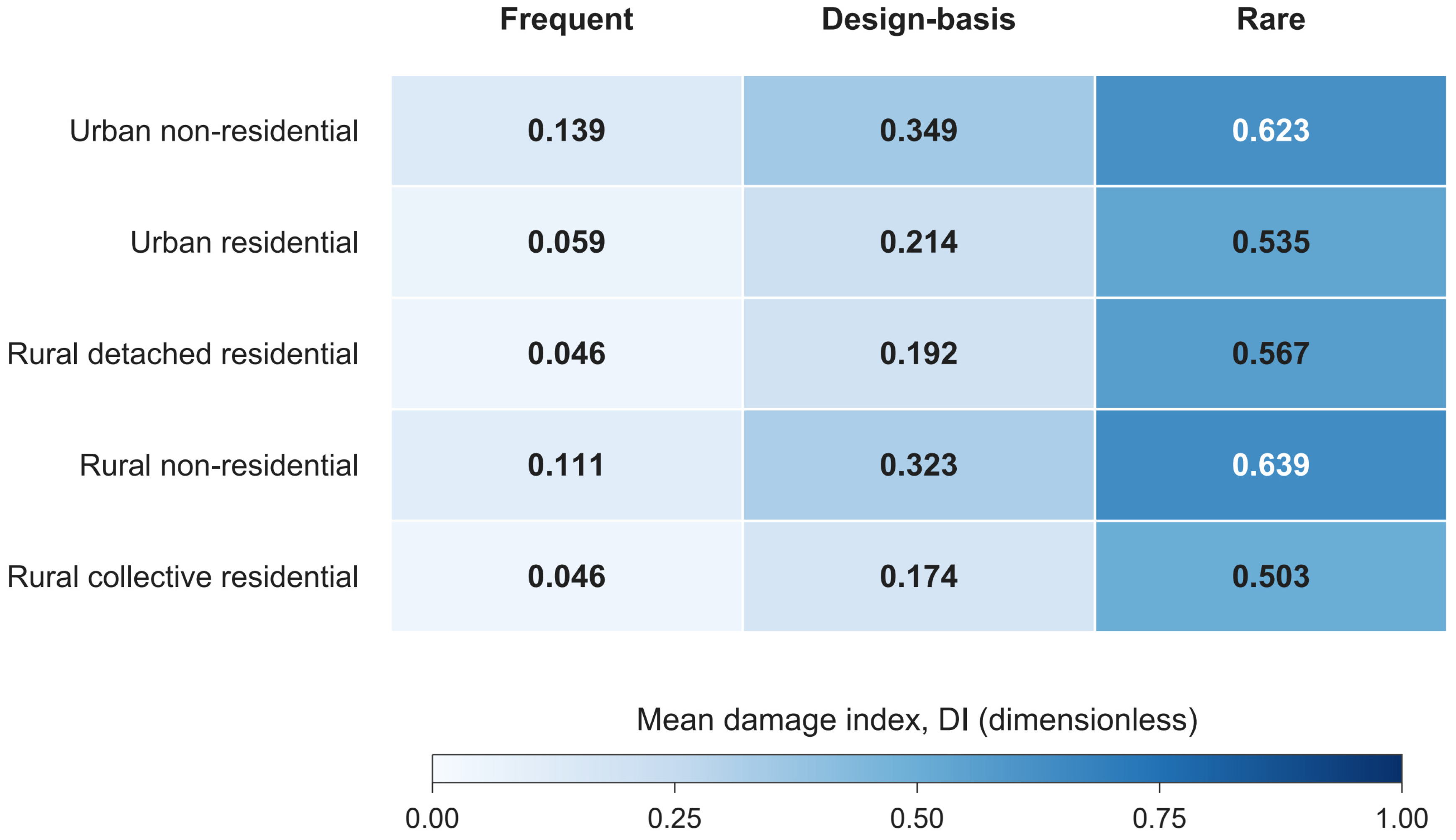
As shown in Figure 7, the mean DI increased with scenario intensity in all five project categories, although conditional damage severity and exposure scale differed substantially among categories. Under the rare earthquake, rural non-residential buildings had the highest mean DI (0.639), followed by urban non-residential, rural detached residential, urban residential, and rural collective residential buildings. Because the rural detached residential category contains more than 1.05 million buildings, its expected Grade 4–5 count under the rare earthquake reached 844,627, representing 80.1% of the category and the largest contribution to the number of highly damaged buildings in the region. The higher mean DIs of rural and urban non-residential buildings indicate greater conditional damage severity, whereas the rural detached residential category represents a much larger exposure.

Figure 7. Mean damage index by project category and earthquake scenario.

4.2. Effects of Building Attributes on Seismic Damage

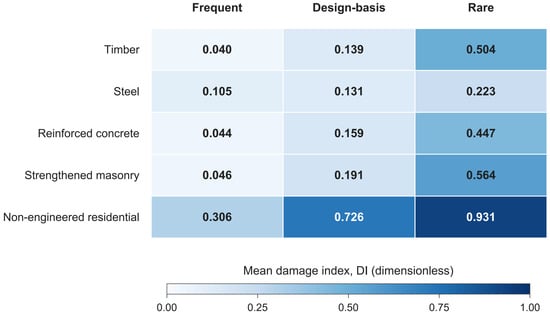
Figure 8 shows that the mean DI increased with scenario intensity for every structural type, although the rate of increase and the upper damage tail differed markedly among systems. Under the rare earthquake, non-engineered residential buildings had a mean DI of 0.931, with 95.8% assigned to Grade 5. The 95.8% proportion is obtained by counting building-level grade assignments over all buildings of this class, not by averaging the class-mean DI. The spread of the inventory-wide Grade 5 share across the three records (6.1–6.4%) indicates the magnitude of input-related uncertainty relative to this parameter-driven vulnerability separation. Strengthened masonry had a mean DI of 0.564, with 78.5% concentrated in Grade 4. Steel, reinforced-concrete, timber, and strengthened-masonry structures exhibited distinct damage patterns dominated by Grade 2, Grade 3, Grades 3–4, and Grade 4, respectively.

Figure 8. Mean damage index by structural type and earthquake scenario.

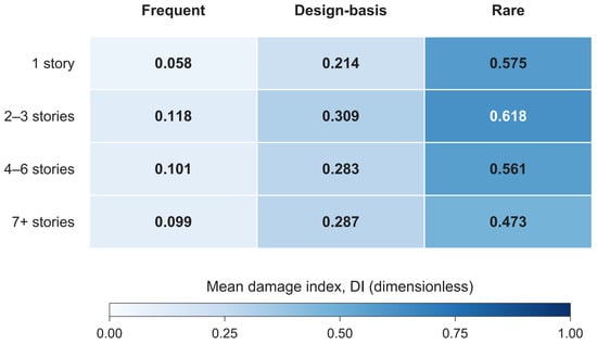
The story-group comparison in Figure 9 exhibits a distinctly nonmonotonic pattern: under the rare earthquake, two- to three-story buildings had the highest mean DI (0.618), followed by one-story, four- to six-story, and seven-story-or-taller buildings. This pattern should not be interpreted as evidence that taller buildings are safer, because the story groups differ in structural system, occupancy, floor area, construction period, spatial location, and spectral demand. In particular, one-story buildings account for 90.8% of the inventory and therefore dominate regional statistics, whereas the smaller population of mid- and high-rise buildings is more likely to be controlled by spectral acceleration than by PGA. Table 5 cross-tabulates structural type within each story group so that this compositional confound can be assessed directly. Within the two- to three-story group, strengthened masonry and non-engineered residential buildings together account for 77.8% of the stock (60,686 of 78,032 buildings), whereas reinforced-concrete buildings dominate the seven-or-more-story group (10,481 of 12,388, 84.6%), confirming that the story-group contrast largely tracks the structural type.

Figure 9. Mean damage index for different story groups under the three earthquake scenarios.

Table 5. Distribution of structural types within each story group.

Story Group	Timber	Steel	RC	Strengthened Masonry	Non-Engineered Residential	Total
1 story	29,187	21,464	25,995	1,210,844	67,094	1,354,584
2–3 stories	583	1565	15,198	40,754	19,932	78,032
4–6 stories	8	263	14,238	24,973	7024	46,506
7+ stories	2	49	10,481	320	1536	12,388
Total	29,780	23,341	65,912	1,276,891	95,586	1,491,510

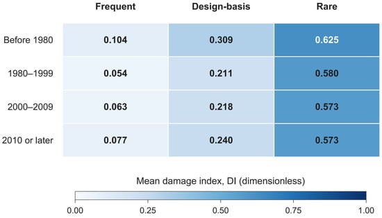
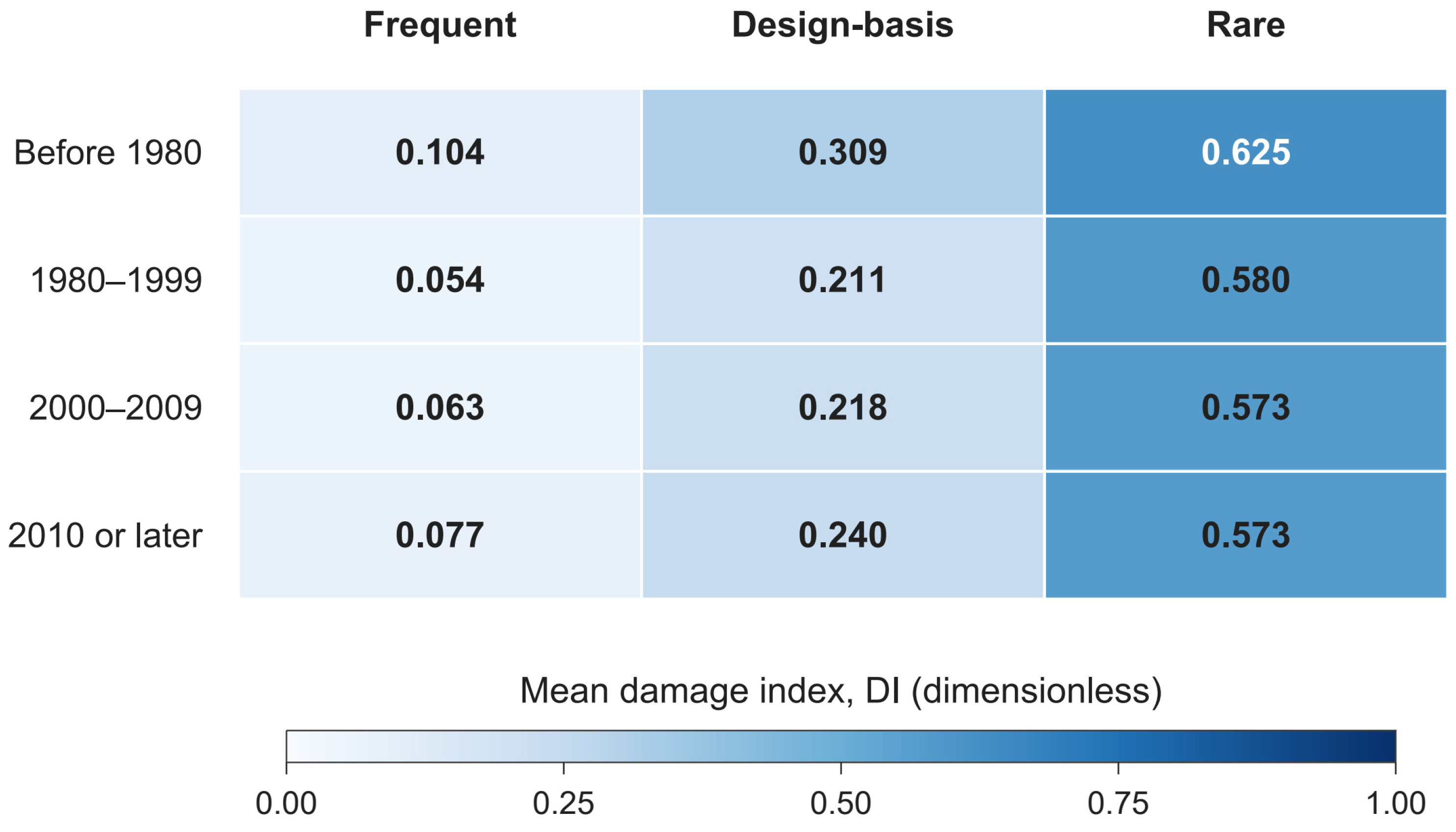
Figure 10 shows that buildings constructed before 1980 had the highest mean DI under the rare earthquake, although this group contained only 2312 buildings. This group represents only 0.15% of the inventory, is spatially clustered, and is internally heterogeneous in structural type; the comparison is therefore reported for completeness, and no inference about the pre-1980 cohort is drawn from this small subsample. Building-count mean DIs were similar for buildings constructed in 1980–1999, 2000–2009, and 2010 or later. Floor-area weighting changes the relative weight of the larger buildings in each period group, so construction-period comparisons should be interpreted jointly with the structural-composition differences among periods. Construction-period effects must be interpreted after controlling for structural type and PGA.

Figure 10. Mean damage index by construction-period group under the three earthquake scenarios.

4.3. Spatial Characteristics of Building-Stock Damage

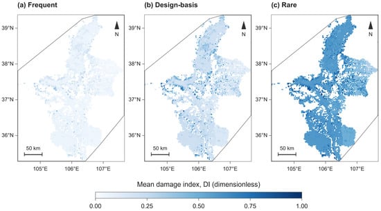
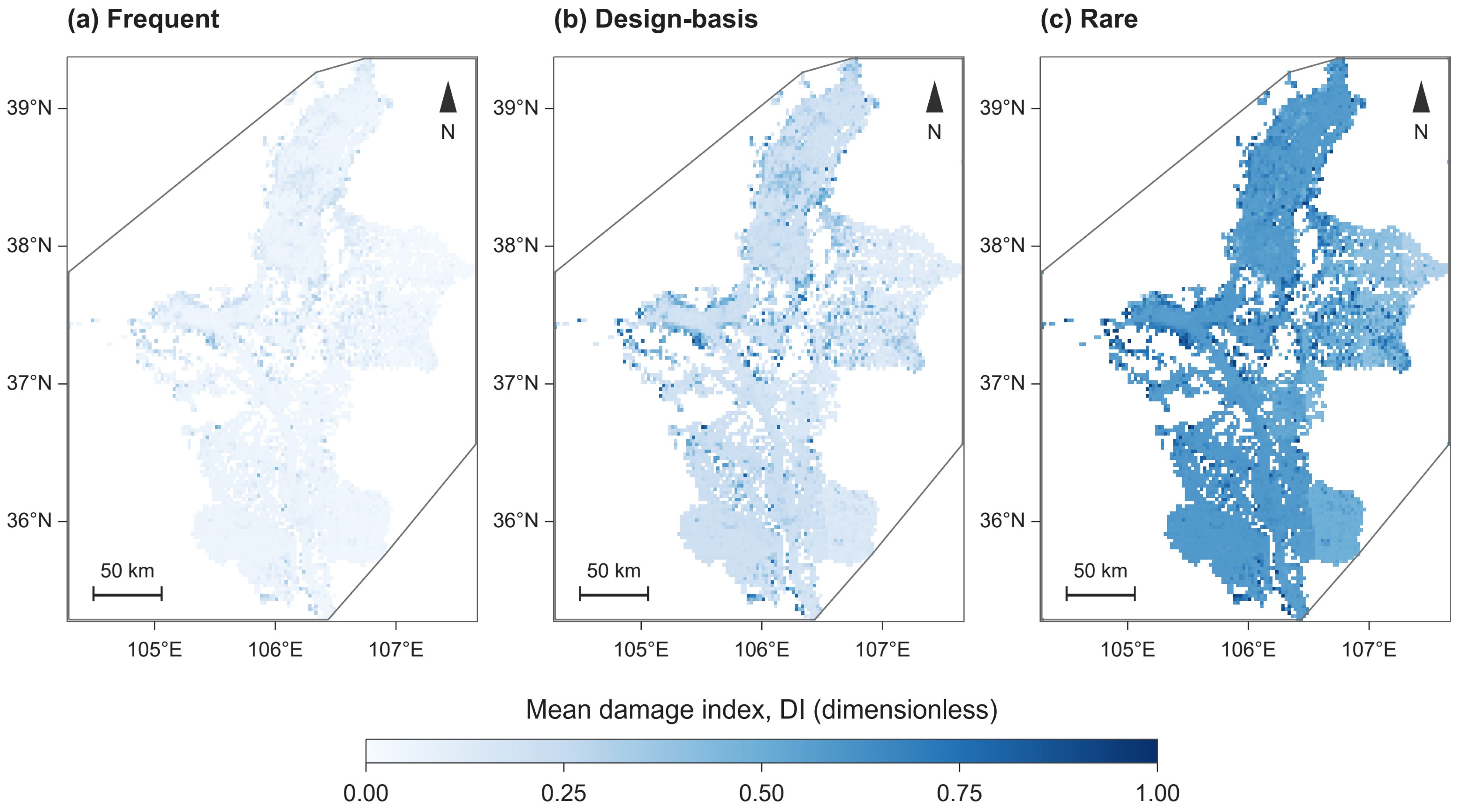
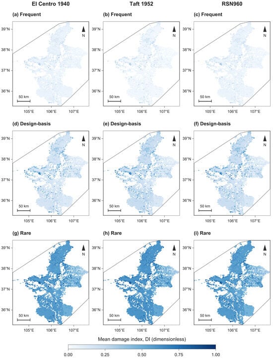
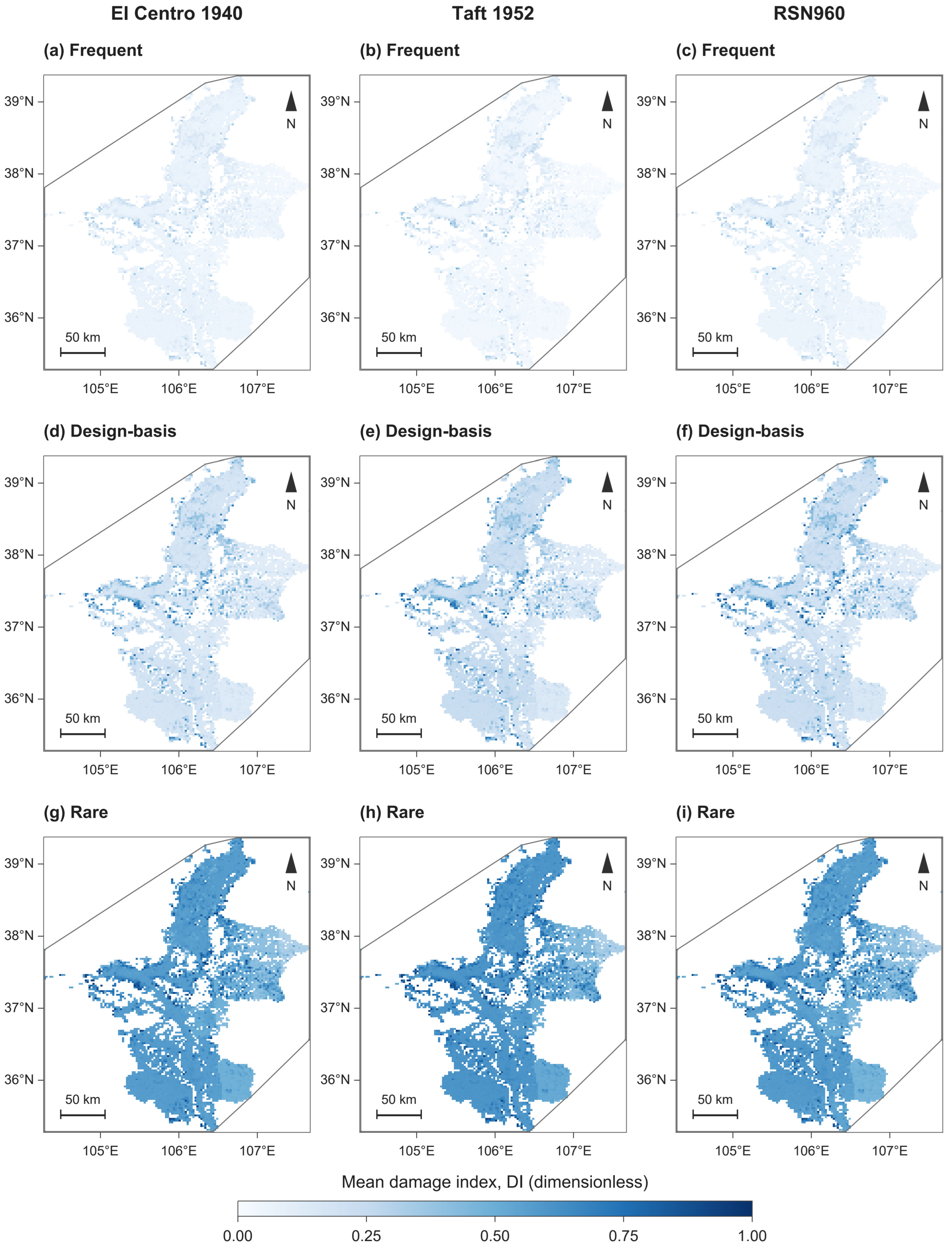
Figure 11 shows that, as scenario intensity increased, the 0.025° grid maps of mean DI evolved from scattered low-intensity patches into continuous high-value belts. When the results are disaggregated by the three ground-motion records, Figure 12 further shows that the broad spatial pattern remains similar within a given scenario, while local damage intensity and the extent of high-value areas vary among records. Detailed indicators are shown in Table 6. Global Moran’s I values were 0.429, 0.435, and 0.586 for the frequent, design-basis, and rare earthquakes, respectively; all 499-permutation tests yielded p = 0.002, rejecting the null hypothesis of spatial randomness. The rare earthquake produced the highest I value, indicating that once large numbers of buildings cross nonlinear damage thresholds, local PGA and spatially clustered stocks of similar buildings jointly form more continuous damage zones. The Spearman correlation between DI and building-specific design PGA increased from 0.366 under the frequent earthquake to 0.524 under the rare earthquake, showing that the spatial hazard gradient maps more directly onto the damage gradient under stronger scenarios. The correlation remained well below 1, however, indicating that structural composition cannot be neglected.

Figure 11. Spatial distributions of the three-record mean DI under the frequent, design-basis, and rare earthquake scenarios.

Figure 12. Nine-gridded damage fields for the three earthquake scenarios and three ground-motion records. Rows compare record effects, and columns compare scenario transitions.

Table 6. Spatial association and overlap of high-value grid sets at two spatial scales.

Scenario	Moran’s I/0.025°	Moran’s I/0.05°	ρ(DI, PGA)	ρ(DI, Record Range)	Top-Decile Jaccard Index	Gini/Number of Grade 4–5 Buildings
Frequent earthquake	0.429	0.438	0.366	0.243	0.198	0.989
Design-basis earthquake	0.435	0.471	0.442	0.730	0.352	0.835
Rare earthquake	0.586	0.718	0.524	−0.290	0.039	0.726

After the grid was enlarged to 0.05°, Moran’s I became 0.438, 0.471, and 0.718 for the frequent, design-basis, and rare earthquakes, respectively. The direction of positive spatial association remained unchanged, but I under the rare earthquake increased by 0.133, indicating that spatial aggregation smooths local outliers and strengthens large-scale continuity. Spatial clustering is therefore treated here as a robust qualitative finding, whereas an I value or hotspot boundary at a single scale is not regarded as an intrinsic geographical property.

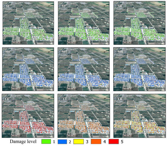
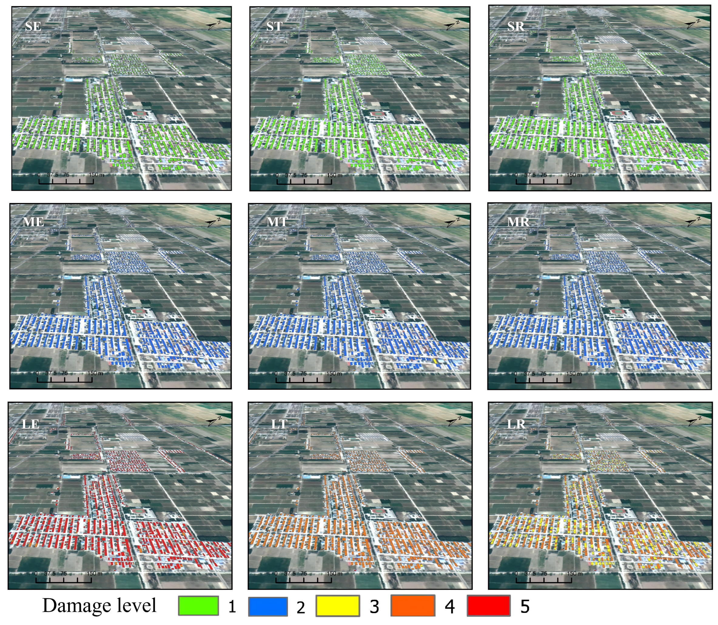
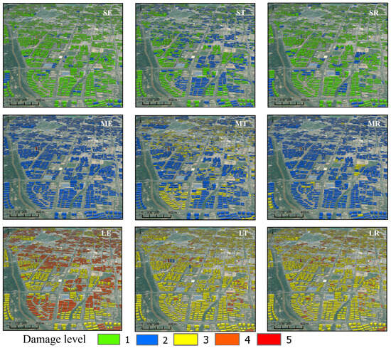
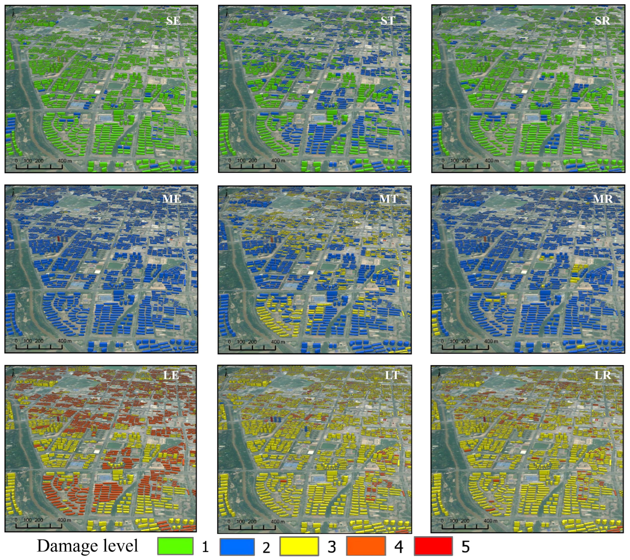
Grid aggregation is necessary for regional comparison, but it can obscure damage contrasts among individual buildings within rural settlements and urban neighborhoods. To bridge the regional and building scales, the spatial distributions of the five damage grades were visualized for a selected rural area and a selected urban area under the nine scenario–record combinations (Figure 13 and Figure 14). Both visualizations use a fixed spatial extent, viewing geometry, and damage-grade color scale, allowing changes in damage severity and spatial clustering to be compared consistently across scenarios and records.

Figure 13. Building-level damage-grade distributions in a selected rural area under nine scenario–record combinations. Rows represent frequent (S), design-basis (M), and rare (L) earthquake scenarios; columns represent the El Centro (E), Taft (T), and RSN960 NORTHR LOS (R) records. The color scale denotes Grades 1–5, from essentially intact to destroyed.

Figure 14. Building-level damage-grade distributions in a selected urban area under nine scenario–record combinations. Rows represent frequent (S), design-basis (M), and rare (L) earthquake scenarios; columns represent the El Centro (E), Taft (T), and RSN960 NORTHR LOS (R) records. The color scale denotes Grades 1–5, from essentially intact to destroyed.

Figure 13 and Figure 14 reveal a clear scenario-dependent progression at the individual-building scale. In the selected rural area, the frequent- and design-basis-earthquake results are nearly uniform and are dominated by Grades 1 and 2, respectively. Under the rare earthquake, the rural damage field becomes markedly record-sensitive: the El Centro result is dominated by Grade 5, the Taft result by Grade 4, and the RSN960 NORTHR LOS result by Grades 3–4. The selected urban area displays greater spatial heterogeneity. Grades 1–2 dominate under the frequent earthquake, Grade 2 remains widespread under the design-basis earthquake with localized Grade 3 clusters, and the rare-earthquake results show broad Grade 3 coverage together with clustered Grade 4–5 buildings. Within these selected examples, the rural settlement therefore exhibits a comparatively uniform but record-sensitive transition, whereas the urban neighborhood retains a more heterogeneous damage mosaic. These building-level visualizations complement the gridded statistics by showing that a similar aggregate DI can correspond to markedly different spatial configurations of damaged buildings and, consequently, different inspection and intervention demands. Because only one rural and one urban area are shown, the comparison is interpreted as an illustration of local response patterns rather than an estimate of the overall rural–urban damage difference.

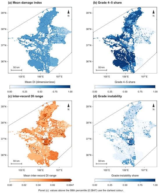
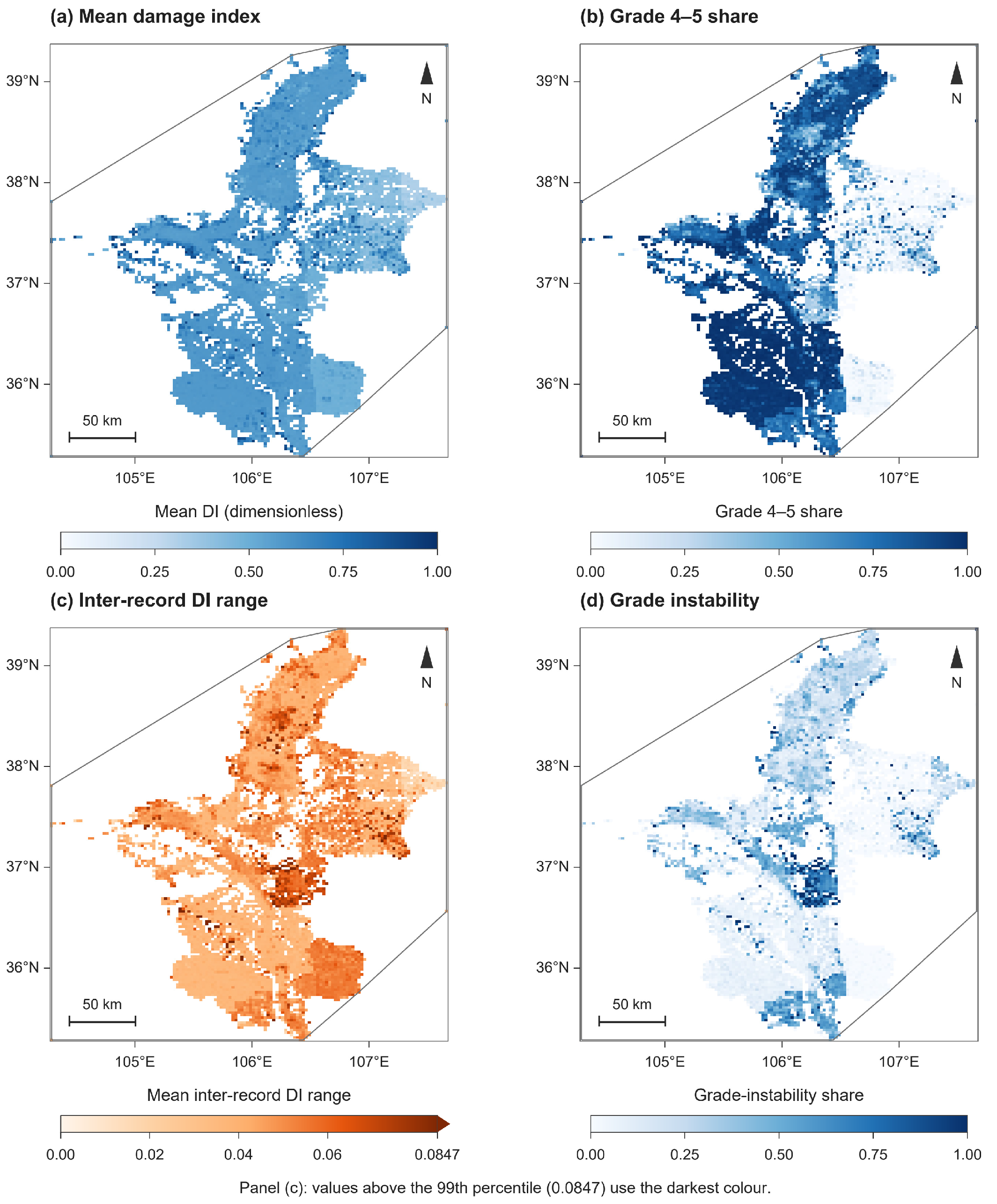
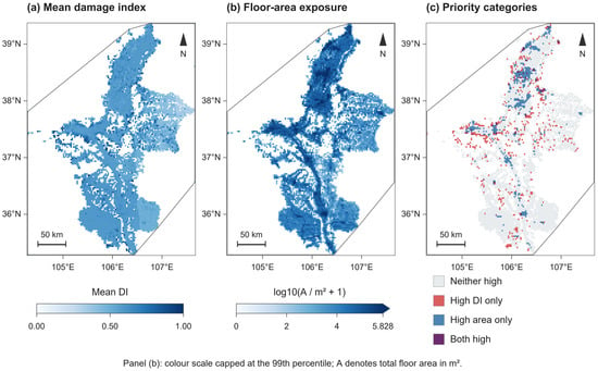
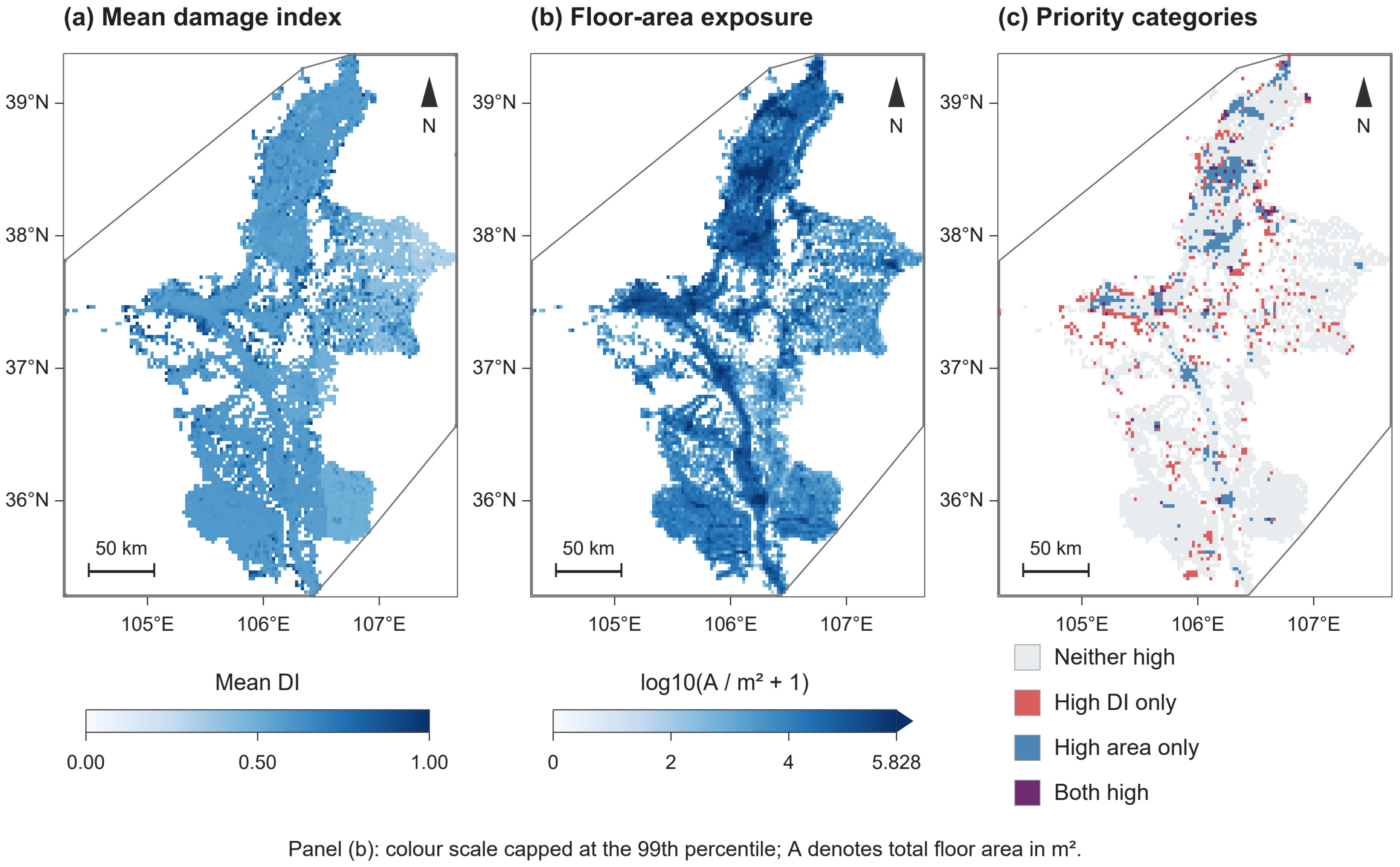
Figure 15 juxtaposes mean DI, the Grade 4–5 exceedance proportion, the three-record DI range, and the damage-grade instability rate under the rare earthquake, visually demonstrating that high-damage and high-record-sensitivity areas do not coincide. The grid-level rank correlation between DI and record-to-record DI range was −0.290, and the Jaccard index between their top-decile grid sets was only 0.039 (each set contains 518 cells; the intersection contains 39 cells and the union 997 cells). Figure 16 further overlays DI and floor-area exposure; the Jaccard index between the top-decile high-DI and high-floor-area grids was likewise only 0.057 (56 of 518 cells in common; union 980 cells). High mean damage, a large potential intervention scale, and sensitivity to record selection therefore constitute three complementary screening dimensions whose high-value sets overlap only weakly in this record set. The grid-level Gini coefficient for the three-record mean number of Grade 4–5 buildings decreased from 0.989 under the frequent earthquake to 0.726 under the rare earthquake, indicating that severe damage spread from a few localized cells to a broader area rather than remaining concentrated in a small number of conventional hotspots. The very high value under the frequent earthquake should be read with care: the three-record mean Grade 4–5 count was only about 362 buildings in total, distributed over 210 of the 6404 populated cells (96.7% of cells contained no Grade 4–5 buildings), and the largest single cell held 12.6% of all Grade 4–5 buildings; the high Gini therefore reflects a sparse distribution with many zero cells rather than a single dominant hotspot. Computed over only the 210 non-zero cells, the Gini coefficient equals 0.666; all values in this paragraph were re-verified against the archived gridded dataset during revision.

Figure 15. Mean DI, Grade 4–5 exceedance proportion, three-record DI range, and damage-grade instability rate under the rare earthquake scenario.

Figure 16. Mean DI, floor-area exposure, and bivariate priority screening under the rare earthquake scenario. Red denotes high damage, blue high exposure, and purple their overlap.

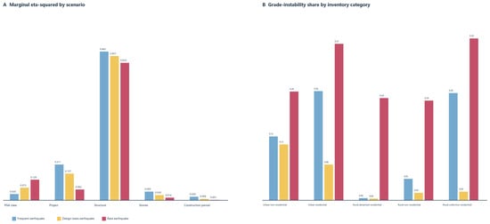
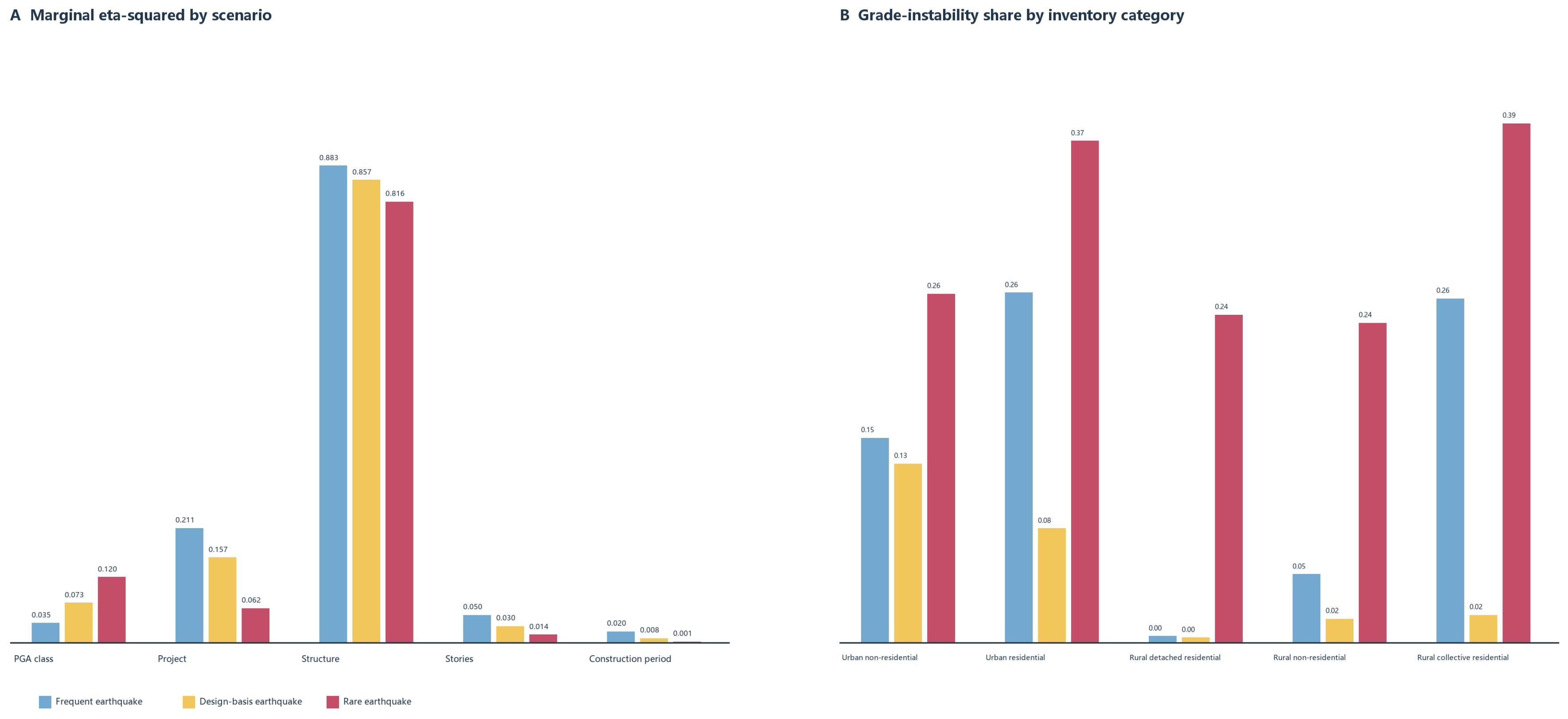
As shown in Figure 17A, the marginal η² for structural type was 0.883, 0.857, and 0.816 under the frequent, design-basis, and rare earthquakes, respectively, substantially exceeding the 0.035–0.120 range for the PGA group alone. The η² of the joint PGA-by-structural-type stratification remained between 0.950 and 0.962, indicating that the combination of hazard and structural vulnerability describes most of the variation within the inventory. Because structural type, occupancy, number of stories, and spatial PGA are not orthogonal by design, these results cannot be decomposed into a net causal effect of structural type or a statistical interaction effect.

Figure 17. Marginal η² by project category, structural type, story group, construction period, and PGA group, together with damage-grade instability rates for the five building categories.

Figure 17B further shows that building-level DI correlations among the three records were consistently high (0.967–0.990), yet the damage-grade instability rate changed from 4.9% under the frequent earthquake and 2.5% under the design-basis earthquake to 25.7% under the rare earthquake. These observations are not contradictory: even when the overall ranking of continuous DI is stable, small record-to-record differences can move buildings near the 0.10, 0.30, 0.55, and 0.85 thresholds into different grades. Under the rare earthquake, the instability rates for urban residential and rural collective residential buildings reached 37.2% and 38.5%, respectively, exceeding the 24.3% rate for rural detached residential buildings.

4.4. Comparison Across Earthquake Scenarios

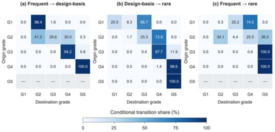
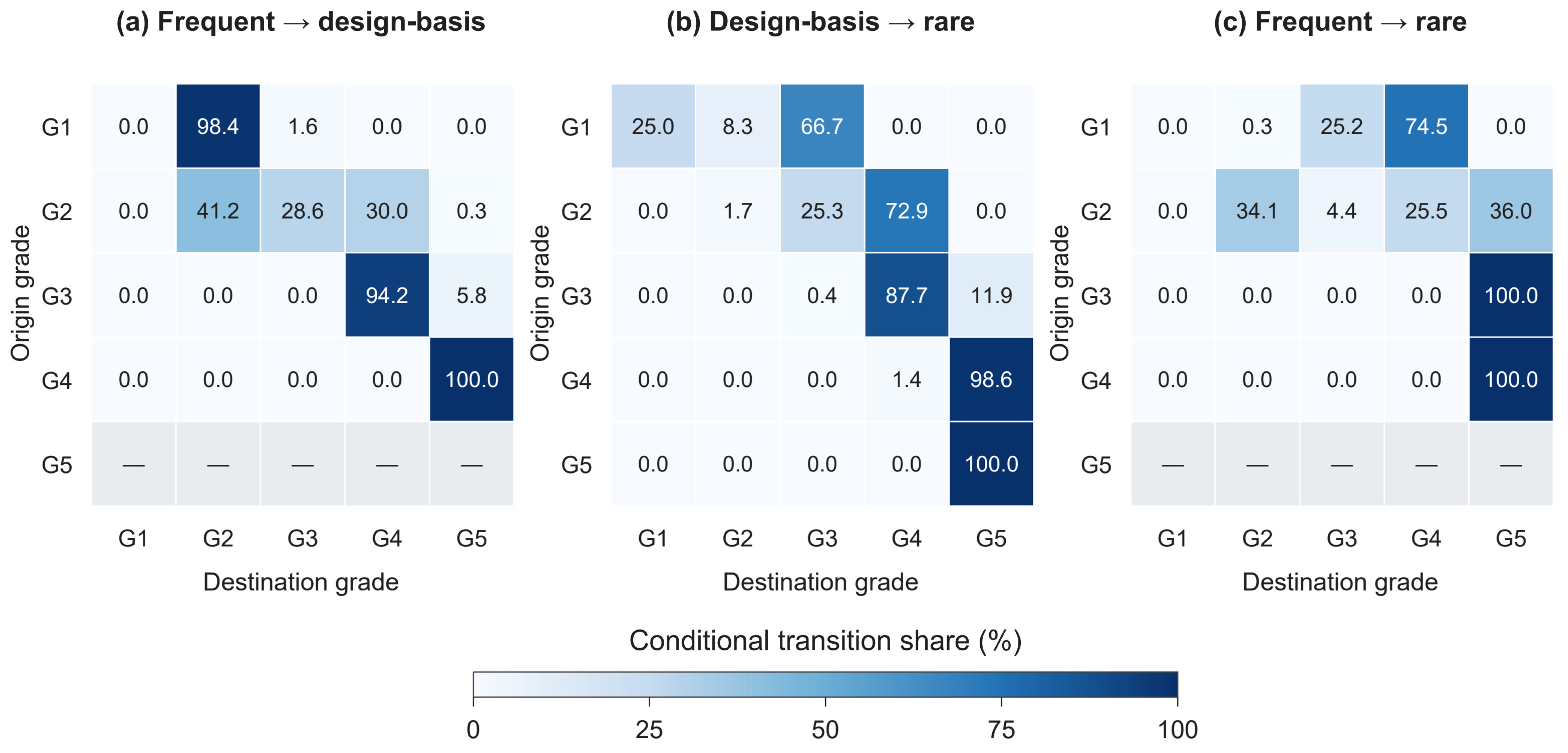
The scenario-transition matrices in Figure 18 show that, after a representative damage grade was assigned to each building from its three-record mean DI, 98.4% of buildings in Grade 1 under the frequent earthquake transitioned to Grade 2 under the design-basis earthquake. From the design-basis to the rare earthquake, 72.9% of Grade 2 buildings transitioned directly to Grade 4, 87.7% of Grade 3 buildings transitioned to Grade 4, and 98.6% of Grade 4 buildings transitioned to Grade 5. When the frequent and rare earthquakes were compared directly, 74.5% of the buildings originally in Grade 1 transitioned to Grade 4. These results demonstrate that increasing the scenario intensity does not simply translate the DI distribution; rather, it causes nonlinear transitions controlled jointly by the structural backbone curves and damage thresholds. The direct transition of 74.5% of the originally Grade 1 buildings to Grade 4 under the rare earthquake reflects buildings whose rare-earthquake demand exceeds first the yield capacity and then approaches the collapse capacity of the story; the likelihood of such threshold crossings is governed by the overstrength and ductility margins of each structural type, and Table 7 quantifies this link: the direct frequent-to-rare Grade 1-to-4 flow is 80.0% for strengthened masonry but 9.7% for timber and at most 0.3% for steel and reinforced-concrete buildings; non-engineered residential buildings are assigned to Grade 5 in essentially all cases once their mean DI crosses the rare-earthquake thresholds. The transition percentages are conditional on the scenario pair considered and do not represent probabilities of event occurrence.

Figure 18. Scenario-transition matrices for damage grades assigned from the three-record mean DI; percentages are conditional on the initial grade.

Table 7. Key conditional transition shares by structural type (grades assigned from the three-record mean DI of each scenario). Conditional shares based on very small origin populations (e.g., Grade 1 non-engineered buildings under the frequent earthquake) should be read with that limitation in mind; dashes denote empty origin sets.

Structure	n	P(1 → 2), Frequent → Design-Basis	P(2 → 4), Design-Basis → Rare	P(3 → 4), Design-Basis → Rare	P(4 → 5), Design-Basis → Rare	P(1 → 4), Frequent → Rare	Grade 4–5 Share Under Rare Earthquake
All	1,491,510	0.985	0.729	0.877	0.986	0.745	0.752
Timber	29,780	1.000	0.097	0.000	—	0.097	0.097
Steel	23,341	1.000	0.000	0.000	—	0.000	0.000
RC	65,912	1.000	0.002	0.197	—	0.003	0.003
Strengthened masonry	1,276,891	0.983	0.796	1.000	0.008	0.800	0.801
Non-engineered residential	95,586	1.000	0.721	0.520	1.000	0.000	0.999

5. Discussion

The multi-scenario assessment covers the complete urban and rural building stock of Ningxia and retains the same inventory and full factorial combination of three records at each of the three seismic fortification levels. It therefore permits direct comparison of scenario transitions, building exposure, and record sensitivity. The principal value of this study lies not in reporting a single regional mean DI, but in separating hazard, vulnerability, and exposure into traceable components of the analysis. Building-specific target PGA represents spatial variation in the scenario hazard; structural type, number of stories, and construction period enter the response model; building count and floor area describe exposure; and the range across the three records describes limited record sensitivity. This organization is consistent with the modular philosophy of OpenQuake and city-scale nonlinear time-history frameworks [4,12], while further emphasizing that different metrics address different engineering questions. High mean DI indicates damage severity, a high Grade 5 proportion indicates tail consequences, a large number of damaged buildings indicates inspection workload, a large damaged floor area indicates potential asset and sheltering pressures, and a large record range indicates instability of the result.

Building-specific PGA scaling avoids applying the same input amplitude to all buildings in the region and allows spatial variation in seismic design intensity to enter the response analysis. The relatively stable mean DI but widely varying Grade 4–5 proportion under the rare earthquake shows that, even after PGA is controlled, spectral and time-history characteristics can change the number of buildings crossing damage thresholds. However, three seed records are insufficient to represent the potential distributions of magnitude, source-to-site distance, site condition, and spectral shape in Ningxia, and linear PGA scaling does not ensure spectral compatibility over structure-relevant periods [33,34]. A more robust approach would select a statistically meaningful suite of records based on hazard deaggregation or a target conditional spectrum, report the mean, variance, and mismatch of target and record spectra, and constrain scale factors [35,36,37,38]. Such an approach would require a more comprehensive investigation of site conditions and seismic hazards across Ningxia. Until such an expanded suite is analyzed, the results of this study are conditional scenario estimates for the three selected record pairs, and the reported record range should be read as a descriptive sensitivity measure within this set rather than as a quantification of the epistemic uncertainty of regional seismic damage in Ningxia.

Non-engineered residential buildings account for only 6.4% of the inventory but are highly concentrated in Grade 5 under the rare earthquake. This low-prevalence, high-vulnerability group is suitable for model verification, field sampling, and priority retrofit assessment. Strengthened masonry accounts for 85.6% of all buildings and is concentrated mainly in Grade 4 under the rare earthquake. This group has relatively lower consequences per building but extremely large aggregate exposure and is therefore more suitable for zoned, tiered, and standardized large-scale retrofit programs. Although rural detached residential buildings do not have the highest mean DI, their expected Grade 4–5 count exceeds 840,000, showing that governance priorities cannot be ranked by mean DI alone. Urban non-residential and steel buildings represent relatively small shares by count but relatively large shares by floor area and may include industrial, commercial, or public-service functions. Because the current dataset lacks the attributes required for loss estimation—replacement cost by structural type and occupancy, repair-cost ratios by damage grade, and functional-importance and business-interruption information—economic loss cannot be inferred directly from floor area. Adding building function, replacement cost, repair-cost functions, and recovery time in future work would allow the present damage results to be converted into direct-loss and downtime estimates and would help identify facilities that are few in number but critical in function.

Moran’s I remains positive and significant from the frequent to the rare earthquake, demonstrating that the spatial structure of damage is not a random mosaic of more than one million independent building responses. At least three processes contribute to this pattern: design-PGA zoning gives neighboring buildings a shared hazard level; urban–rural development and construction periods create spatial clusters of structural types; and regular-grid aggregation smooths neighboring building responses into regional means. The higher Moran’s I and lower Gini coefficient for Grade 4–5 building counts under the rare earthquake reveal two apparently opposing but compatible processes: damage intensity forms more continuous high-value belts, while the number of severely damaged buildings spreads from a few cells to a broader area. Stronger clustering therefore does not imply that consequences are more concentrated. The increase in rare-earthquake Moran’s I from 0.586 at 0.025° to 0.718 at 0.05° demonstrates sensitivity to the modifiable areal unit problem [32]. Recalculation at two scales confirms the robust direction of positive autocorrelation but does not imply that hotspot boundaries remain invariant at other scales. In applications, grid resolution should match the decision unit: coarse grids may support regional resource allocation, whereas neighborhood screening should return to individual buildings or administrative units. Formal local LISA or hotspot testing should also address multiple comparisons, edge cells, and administrative-boundary effects [39]. A direct test of the three candidate processes compares the Moran’s I of the damage maps, computed on the same 5173-cell grid and with the same rook weights, with the Moran’s I of the design-PGA field and of the rural-project share: the design-PGA field has I = 0.874 and the rural-project share I = 0.679, against 0.429–0.586 for the damage fields (all p = 0.002; excluding the 62 isolated cells changes the damage values only to 0.442, 0.448, and 0.596). The ordering indicates that a large part of the damage clustering is inherited from the hazard zoning and the urban–rural composition, with the response analysis attenuating rather than creating the spatial structure.

Treating the most uncertain locations as the most severely affected would therefore misallocate resources. High-DI, low-range cells can be prioritized for engineering intervention; high-DI, high-range cells require intervention and verification in parallel; and low-DI, high-range cells should first receive an expanded ground-motion suite and model checks. This classification is a screening framework for conditional scenarios, not a risk ranking based on occurrence rates, casualties, or asset losses. A three-dimensional priority matrix is recommended. The first dimension is damage severity, represented by mean DI, Grade 5 proportion, or Grade 4–5 proportion; the second is exposure scale, represented at minimum by both building count and floor area; and the third is record sensitivity, represented by the three-record range or, for an expanded record set, a quantile range. Areas with high damage, high exposure, and low sensitivity can be prioritized for retrofit and emergency-resource planning. Areas with high damage and high sensitivity require additional records and model verification alongside intervention, whereas areas with low mean damage but high sensitivity are better suited for initial uncertainty investigation. Under the rare earthquake, the overlap between the top-decile high-DI and high-record-range grid sets was limited (Jaccard index 0.039; 39 of 518 cells in common), as was the overlap with the high-floor-area set (Jaccard index 0.057). As a concrete implementation, the three dimensions can be applied as a simple three-tier rule rather than a weighted score: (i) cells in the top decile of mean DI with low record sensitivity enter the engineering-intervention list directly; (ii) cells in the top decile of both mean DI and record sensitivity enter the intervention list with a mandatory model-and-record verification step; and (iii) remaining cells whose record range exceeds the 90th percentile are queued for expanded ground-motion analysis before intervention decisions. The dimensions are deliberately left unweighted because the appropriate trade-off among severity, exposure, and uncertainty depends on the decision context.

6. Conclusions

This study established a building-level, multi-scenario, multi-record workflow for physics-based seismic damage simulation and spatial statistics covering approximately 1.49 million buildings across Ningxia. The results show that apparently stable regional mean DIs can coexist with pronounced differences in damage-grade composition and spatial clustering. A three-dimensional screening framework based on damage severity, exposure scale, and record sensitivity is proposed. The main conclusions are as follows.

• A building-level seismic damage assessment workflow covering 1,491,510 buildings in Ningxia was developed for multiple scenarios and ground-motion records. Full-factorial nonlinear time-history analyses were completed for three sets of bidirectional horizontal ground motions under frequent, design-basis, and rare earthquake scenarios, producing 13,423,590 building–scenario–record results and a one-to-one linkage among building attributes, damage responses, and spatial geometries.
• The building-count-averaged regional DIs under the frequent, design-basis, and rare earthquakes were 0.063, 0.222, and 0.576, respectively. The dominant damage grade shifted from Grade 1 to Grade 2 and then to Grade 4, showing that increasing scenario intensity causes nonlinear transitions across damage thresholds. Under the rare earthquake, 74.23% of buildings were in Grades 4–5 and the three-record mean number of Grade 5 buildings was approximately 92,082. The floor-area-weighted DIs under the frequent and design-basis earthquakes were 1.68 and 1.31 times the building-count means, indicating that building-count and floor-area summaries weight the same damage field differently and should be reported together.
• Building vulnerability and exposure scale have different implications for risk governance. Non-engineered residential buildings account for only 6.4% of the inventory, but 95.8% were assigned to Grade 5 under the rare earthquake, indicating that model verification and field screening should be prioritized. Strengthened masonry accounts for 85.6% of the inventory, and rural detached residential buildings account for 70.7%; approximately 844,627 buildings in the latter category reached Grades 4–5, making them the principal contributor to the number of highly damaged buildings. Retrofit prioritization should therefore consider damage severity, damaged-building count, and damaged floor area together.
• Under the rare earthquake, the regional mean DI across the three records ranged only from 0.563 to 0.598, whereas the Grade 4–5 proportion ranged from 60.4% to 83.6%, showing that similar regional means do not imply stable damage-grade composition. Spatial autocorrelation was significant: Moran’s I on the 0.025° grid increased from 0.429 under the frequent earthquake to 0.586 under the rare earthquake, reflecting both the emergence of more spatially continuous damage zones as larger numbers of buildings cross damage thresholds and the underlying spatial structure of hazard and building types. The Jaccard index between the top-decile high-DI and high-record-range grids under the rare earthquake was only 0.039 (39 of 518 cells in common). Within the present three-record conditional scenarios, damage severity, exposure scale, and record sensitivity should therefore be treated as complementary screening dimensions, with distinct intervention and verification strategies applied to high-consequence and high-uncertainty areas.

References

- Cornell, C.A. Engineering seismic risk analysis. Bull. Seismol. Soc. Am. 1968, 58, 1583–1606. [Google Scholar] [CrossRef] [Scilit]
- Mouroux, P.; Le Brun, B. Presentation of RISK-UE Project. Bull. Earthq. Eng. 2006, 4, 323–339. [Google Scholar] [CrossRef] [Scilit]
- Lagomarsino, S.; Giovinazzi, S. Macroseismic and mechanical models for the vulnerability and damage assessment of current buildings. Bull. Earthq. Eng. 2006, 4, 415–443. [Google Scholar] [CrossRef] [Scilit]
- Silva, V.; Crowley, H.; Pagani, M.; Monelli, D.; Pinho, R. Development of the OpenQuake engine, the Global Earthquake Model’s open-source software for seismic risk assessment. Nat. Hazards 2014, 72, 1409–1427. [Google Scholar] [CrossRef] [Scilit]
- Federal Emergency Management Agency. Hazus Earthquake Model Technical Manual, Hazus 5.1; FEMA: Washington, DC, USA, 2022.
- Barbat, A.H.; Carreño, M.L.; Pujades, L.G.; Lantada, N.; Cardona, O.D.; Marulanda, M.C. Seismic vulnerability and risk evaluation methods for urban areas: A review with application to a pilot area. Struct. Infrastruct. Eng. 2010, 6, 17–38. [Google Scholar] [CrossRef] [Scilit]
- Fayjaloun, R.; Negulescu, C.; Roullé, A.; Auclair, S.; Gehl, P.; Faravelli, M. Sensitivity of earthquake damage estimation to the input data (soil characterization maps and building exposure): Case study in the Luchon Valley, France. Geosciences 2021, 11, 249. [Google Scholar] [CrossRef] [Scilit]
- Gómez Zapata, J.C.; Pittore, M.; Cotton, F.; Lilienkamp, H.; Shinde, S.; Aguirre, P.; Santa María, H. Epistemic uncertainty of probabilistic building exposure compositions in scenario-based earthquake loss models. Bull. Earthq. Eng. 2022, 20, 2401–2438. [Google Scholar] [CrossRef] [Scilit]
- Lu, X.; Han, B.; Hori, M.; Xiong, C.; Xu, Z. A coarse-grained parallel approach for seismic damage simulations of urban areas based on refined models and GPU/CPU cooperative computing. Adv. Eng. Softw. 2014, 70, 90–103. [Google Scholar] [CrossRef] [Scilit]
- Xiong, C.; Lu, X.; Guan, H.; Xu, Z. A nonlinear computational model for regional seismic simulation of tall buildings. Bull. Earthq. Eng. 2016, 14, 1047–1069. [Google Scholar] [CrossRef] [Scilit]
- Xiong, C.; Lu, X.; Lin, X.; Xu, Z.; Ye, L. Parameter determination and damage assessment for THA-based regional seismic damage prediction of multi-story buildings. J. Earthq. Eng. 2017, 21, 461–485. [Google Scholar] [CrossRef] [Scilit]
- Lu, X.; McKenna, F.; Cheng, Q.; Xu, Z.; Zeng, X.; Mahin, S.A. An open-source framework for regional earthquake loss estimation using the city-scale nonlinear time history analysis. Earthq. Spectra 2020, 36, 806–831. [Google Scholar] [CrossRef] [Scilit]
- Lu, X.; Tian, Y.; Wang, G.; Huang, D. A numerical coupling scheme for nonlinear time history analysis of buildings on a regional scale considering site–city interaction effects. Earthq. Eng. Struct. Dyn. 2018, 47, 2708–2725. [Google Scholar] [CrossRef] [Scilit]
- Nievas, C.I.; Pilz, M.; Prehn, K.; Schorlemmer, D.; Weatherill, G.; Cotton, F. Calculating earthquake damage building by building: The case of the city of Cologne, Germany. Bull. Earthq. Eng. 2022, 20, 1519–1565. [Google Scholar] [CrossRef] [Scilit] [PubMed]
- Wang, F.; Zhang, Y.; Lin, X.; Ba, Z. City-scale buildings damage estimation based on broadband physics-based ground motion simulation of 2021 Ms 6.4 Yangbi, China, earthquake. Earthq. Spectra 2024, 40, 446–468. [Google Scholar] [CrossRef] [Scilit]
- Yuan, X.; Lin, X.; Dou, A.; Wang, S.; Zhang, X.; Xiao, B.; Liu, Z. Rapid assessment of building seismic damage based on pre-earthquake high-resolution images and seismic simulation, taking the Luding M6.8 earthquake in Sichuan as an example. Chin. J. Geophys. 2023, 66, 1438–1447. [Google Scholar]
- Skalomenos, K.; Chen, D.; Lin, X.; Morfidis, K. Physics-based seismic vulnerability assessment of aging building stocks at city scale. Bull. Earthq. Eng. 2025, 23, 4391–4428. [Google Scholar] [CrossRef] [Scilit]
- Chen, Z.; Yuan, X.; Lin, X.; Dou, A.; Wang, Y. Dynamic emergency assessment of earthquake disaster using multi-source data: A case study of MS6.8 Dingri Earthquake. Chin. J. Geophys. 2026, 69, 265–277. [Google Scholar] [CrossRef]
- Chen, X.; Lin, X.; Zhang, L.; Skalomenos, K.A. Method for rapidly generating urban damage scenarios under non-uniform ground motion input based on matching algorithms and time history analyses. Soil Dyn. Earthq. Eng. 2022, 152, 107055. [Google Scholar] [CrossRef] [Scilit]
- Lin, X.; Liu, X.; Hui, J.; Shan, W. Assessment on detailed regional seismic damage risk of buildings based on time-history dynamic analyses. Bull. Earthq. Eng. 2024, 22, 2903–2923. [Google Scholar] [CrossRef] [Scilit]
- Burchfiel, B.C.; Zhang, P.; Wang, Y.; Zhang, W.; Song, F.; Deng, Q.; Molnar, P.; Royden, L. Geology of the Haiyuan Fault Zone, Ningxia-Hui Autonomous Region, China, and its relation to the evolution of the Northeastern Margin of the Tibetan Plateau. Tectonics 1991, 10, 1091–1110. [Google Scholar] [CrossRef] [Scilit]
- Middleton, T.A.; Walker, R.T.; Rood, D.H.; Rhodes, E.J.; Parsons, B.; Lei, Q.; Elliott, J.R.; Ren, Z.; Zhou, Y. The tectonics of the western Ordos Plateau, Ningxia, China: Slip rates on the Luoshan and East Helanshan Faults. Tectonics 2016, 35, 2754–2777. [Google Scholar] [CrossRef] [Scilit]
- Guo, Z.; Lu, R.; Liu, G.; Wang, Y.; Du, P.; Yang, X.; Wu, X.; Wang, K.; Sun, X.; Xu, F.; et al. Seismic risk study based on 3D active fault model of the Ningxia area, northeastern margin of Tibetan Plateau. Geoenviron. Disasters 2026, 13, 29. [Google Scholar] [CrossRef] [Scilit]
- GB 18306-2015; Seismic Ground Motion Parameters Zonation Map of China. Standards Press of China: Beijing, China, 2015. (In Chinese)
- Silva, V.; Brzev, S.; Scawthorn, C.; Yepes, C.; Dabbeek, J.; Crowley, H. A building classification system for multi-hazard risk assessment. Int. J. Disaster Risk Sci. 2022, 13, 161–177. [Google Scholar] [CrossRef] [Scilit]
- GB 50011-2010; Code for Seismic Design of Buildings, 2016th ed. China Architecture & Building Press: Beijing, China, 2016. (In Chinese)
- Ancheta, T.D.; Darragh, R.B.; Stewart, J.P.; Seyhan, E.; Silva, W.J.; Chiou, B.S.; Wooddell, K.E.; Graves, R.W.; Kottke, A.R.; Boore, D.M.; et al. NGA-West2 Database. Earthq. Spectra 2014, 30, 989–1005. [Google Scholar] [CrossRef] [Scilit]
- Mazzoni, S.; Gregor, N.; Al Atik, L.; Bozorgnia, Y.; Welch, D.P.; Deierlein, G.G. Probabilistic Seismic Hazard Analysis and Selecting and Scaling of Ground-Motion Records; PEER Report 2020/14; Pacific Earthquake Engineering Research Center: Berkeley, CA, USA, 2020. [Google Scholar] [CrossRef] [Scilit]
- Wada, A.; Hirose, K. Elasto-plastic dynamic behaviors of the building frames subjected to bi-directional earthquake motion. J. Struct. Constr. Eng. (Trans. AIJ) 1989, 399, 37–47. [Google Scholar] [CrossRef] [Scilit] [PubMed]
- GB/T 17742-2020; The Chinese Seismic Intensity Scale. State Administration for Market Regulation; Standardization Administration of China: Beijing, China, 2020. (In Chinese)
- Moran, P.A.P. Notes on continuous stochastic phenomena. Biometrika 1950, 37, 17–23. [Google Scholar] [CrossRef] [Scilit]
- Fotheringham, A.S.; Wong, D.W.S. The modifiable areal unit problem in multivariate statistical analysis. Environ. Plan. A 1991, 23, 1025–1044. [Google Scholar] [CrossRef] [Scilit]
- Bommer, J.J.; Acevedo, A.B. The use of real earthquake accelerograms as input to dynamic analysis. J. Earthq. Eng. 2004, 8, 43–91. [Google Scholar] [CrossRef] [Scilit]
- Iervolino, I.; Cornell, C.A. Record selection for nonlinear seismic analysis of structures. Earthq. Spectra 2005, 21, 685–713. [Google Scholar] [CrossRef] [Scilit]
- Baker, J.W. Conditional mean spectrum: Tool for ground-motion selection. J. Struct. Eng. 2011, 137, 322–331. [Google Scholar] [CrossRef] [Scilit]
- Bradley, B.A. A generalized conditional intensity measure approach and holistic ground-motion selection. Earthq. Eng. Struct. Dyn. 2010, 39, 1321–1342. [Google Scholar] [CrossRef] [Scilit]
- Jayaram, N.; Lin, T.; Baker, J.W. A computationally efficient ground-motion selection algorithm for matching a target response spectrum mean and variance. Earthq. Spectra 2011, 27, 797–815. [Google Scholar] [CrossRef] [Scilit]
- Lu, X.; Cheng, Q.; Tian, Y.; Huang, Y. Regional ground-motion simulation using recorded ground motions. Bull. Seismol. Soc. Am. 2021, 111, 825–838. [Google Scholar] [CrossRef] [Scilit]
- Anselin, L. Local indicators of spatial association—LISA. Geogr. Anal. 1995, 27, 93–115. [Google Scholar] [CrossRef] [Scilit]
Disclaimer/Publisher’s Note: The statements, opinions and data contained in all publications are solely those of the individual author(s) and contributor(s) and not of MDPI and/or the editor(s). MDPI and/or the editor(s) disclaim responsibility for any injury to people or property resulting from any ideas, methods, instructions or products referred to in the content. |
© 2026 by the authors. Licensee MDPI, Basel, Switzerland. This article is an open access article distributed under the terms and conditions of the Creative Commons Attribution (CC BY) license.