Correction of Compression Modulus of Deep Cohesive Soil and Settlement Calculation Based on Field Tests in the Haihe Alluvial Plain

Abstract

The compression modulus is a key parameter governing the settlement of bridge foundations. To accurately predict pile-group settlement, this study draws on a high-speed railway bridge project crossing the Haihe Alluvial Plain. Combining field monitoring with theoretical analysis, the compression modulus of clay-bearing strata deeper than 50 m is investigated and state-specific correction factors together with their relation to the liquidity index are proposed. The in-situ compression modulus back-calculated from measured settlement of deep clay is 10.47–22.97 times the laboratory modulus E₀. The correction factor β is closely related to soil consistency: mean β values of 0.585, 0.633, 0.648 and 0.798 are obtained for stiff, firm-to-stiff, plastic and soft clays, respectively. β increases linearly with the liquidity index, showing a strong positive correlation. The sensitivity analysis shows that a deviation of 0.05 in β leads to an error of approximately −17% to +24% in the calculated total settlement, and underestimating β yields unsafe predictions. When the measurement resolution is combined, the overall uncertainty band of β is approximately ±0.06, corresponding to an uncertainty band of approximately −21% to +28% in the calculated total settlement. Recommended values are 0.53–0.65 (stiff), 0.57–0.69 (firm-to-stiff), 0.59–0.71 (plastic) and 0.74–0.86 (soft). Within the 0.5 m disturbed zone below the pile tip, the modulus may be taken as 1.2 E₀ for soft clay, 1.6 E₀ for medium-dense sand and 2.0 E₀ for firm-to-stiff clay. The results provide a parameter basis for the settlement prediction of deep-long pile groups in the Haihe Alluvial Plain.

1. Introduction

The complex and variable topography, high urbanisation density and national railway network strategy have made bridges the optimal engineering solution for a large-scale, efficient and safe high-speed railway network; bridges typically account for 60–90% of such lines. Because high-speed rail requires track irregularity to be controlled within millimetres, post-construction settlement of bridge foundations is the most critical consideration in design and construction, and the accuracy of settlement prediction is therefore paramount. Most bridges use pile foundations. Previous studies have mostly approached the problem through settlement calculation methods [1,2,3]. Building on the Geddes stress solution, Lü et al. derived formulas for the additional stress coefficients induced by circular pile tip resistance and shaft friction using double integration and computed the settlement of bridge pile foundations [4]. Yang et al. proposed a nonlinear settlement method for soft ground based on e–p curves [5] and subsequently presented empirical correction coefficients for the layer-wise summation method [6].

Besides the calculation method, determination of the compressible layer thickness also affects settlement. Two approaches exist: the strain-control method and the stress-control method. Ning has noted that, where geological data are sufficiently detailed, the strain-ratio method (strain control) should be used; otherwise, the stress-ratio method (stress control) is preferable [7]. Cheng, based on the measured settlement of deep-long piles on the Beijing–Shanghai railway, concluded that the compressible-layer thickness from the stress method agrees best with measurements [8]. Su et al., through the comparison of calculations with field monitoring, further confirmed that the compressible layer determined by the stress method (10% of overburden stress) closely matches field observations [9,10].

In addition to the choice of method, the soil compressibility index—the compression modulus—is a key calculation parameter. At present, the compression modulus is commonly obtained from oedometer e–p curves as E_s = (1 + e₁)/a. Luo and Du et al. discussed the appropriate value of e₁ and proposed more reasonable expressions [11,12]; nevertheless, settlement calculated from the laboratory compression modulus still differs significantly from measured values. On this basis, Chen [13] and Dong [14], using the time–space effect principle to characterise the in-situ stress field, obtained compensation factors of 1.42–1.49 for the laboratory modulus (i.e., $E_s=(1.42-1.49)E_0$), and established relations between field and laboratory-derived parameters. Field tests showed that after pile installation the compression modulus of clay increases by 1.10–1.24 times, while that of sandy soils increases by 1.79–2.45 times [15]. Chen, based on eight projects in Shanghai, correlated the laboratory modulus with E₀ [16]. The Hubei Institute of Water Conservancy and Electric Power Survey and Design, through extensive statistical regression of standard penetration tests on clay and silt, established E₀ = 1.0658 N + 7.4306 [17]. Zhou et al., using mucky clay, found that the compression modulus first increases and then decreases with load, and grows with time [18]. Wang proposed a different prediction model for the high-pressure interval of deep strata [19]. Comparisons of test methods show that the laboratory modulus can be more than 25 times lower than the in-situ value [20,21,22].

Internationally, the effects of sampling disturbance and test stress level on soil stiffness have long been recognised. Ladd and DeGroot systematically summarised site characterisation and sample-quality evaluation for soft ground, proposing sample classification by disturbance level to guide the use of laboratory results [23]. Burland pointed out that the stiffness at small strains is more than an order of magnitude higher than that measured in conventional tests, and that sampling disturbance combined with low stress levels causes systematic underestimation [24]. Hardin and Richart, based on elastic wave velocity tests, established modulus-confining stress relations showing that stiffness increases with effective stress, mechanistically explaining why the laboratory modulus of deep soil falls increasingly below the in-situ value with depth [25]. Mayne and Kulhawy [26], studying stress history and the coefficient of earth pressure at rest, further showed that the in-situ stress state of deep strata cannot be reproduced by low-pressure laboratory oedometer tests. For pile-group settlement, Randolph and Wroth developed an elastic framework for the deformation of single and grouped piles under vertical load, [27] and Poulos systematically presented the theory and engineering application of pile settlement calculation [28]; both emphasised that the reliability of the soil modulus controls prediction accuracy and advocated back-analysis of soil parameters using field monitoring to reduce uncertainty.

In summary, domestic and international studies consistently show that the laboratory compression modulus is systematically underestimated owing to sampling disturbance and stress-level mismatch, with the magnitude of underestimation depending on depth and soil consistency; back-analysis from field monitoring is a reliable route to the in-situ stiffness of deep soil. However, existing correction formulas are mostly empirical coefficients for specific regions, and no systematic field basis exists for a consistency-specific correction factor for clay deeper than 50 m in the Haihe Alluvial Plain. Accordingly, this study draws on settlement monitoring along the Tianjin–Cangzhou section of the Beijing–Shanghai high-speed railway, back-analyses the in-situ compression modulus of deep clay from measured compression, calibrates the coefficient β in the depth-correction formula (Equation (14)), analyses its quantitative relation with the liquidity index and proposes state-specific recommended values, validating them using independent monitoring data from a third site (D3). Consequently, we provide a parameter basis for the settlement calculation of deep-long pile groups in similar strata.

2. Project Overview

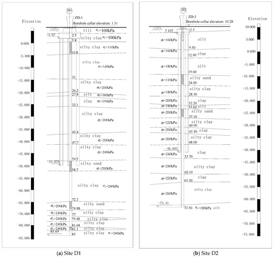
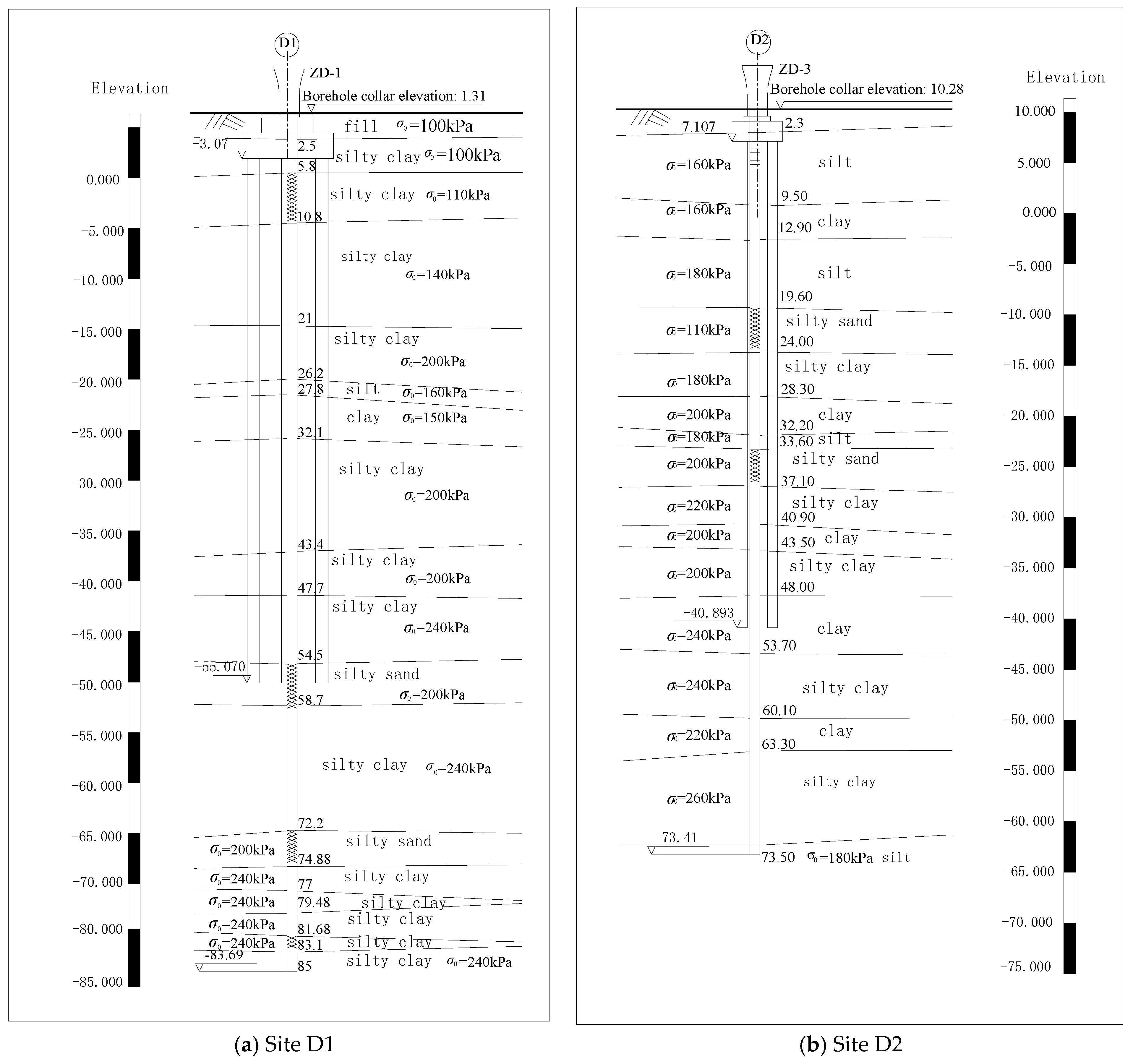
A high-speed railway crosses the Haihe Alluvial Plain region. The strata mainly consist of clay, silty clay, silt, silty sand and fine sand; the stratigraphy beneath the pile tips is shown in Figure 1. Site D1 is located in Tianjin and site D2 in Cangzhou, 115 km apart. The bearing strata beneath the pile tips include silty sand with an allowable bearing capacity of 200 kPa and clay with an allowable bearing capacity of 240 kPa. The research team monitored the settlement of 12 piers along the line; for brevity, two representative sites (D1 and D2) are described and analysed in detail. The number, length and diameter of piles, and the cap geometry and loading are given in Table 1.

Figure 1. Geological cross-section.

Table 1. Parameters of piles and loading.

Site	No. of Piles	Pile Length (m)	Pile Diameter (m)	Spacing (m)	Cap Dimensions (l × w × h, m)	Loadings (kN)
D1	12	52	1.25	3.4	12.5 × 9.1 × 2.5	21,000
D2	8	48	1	3.0 × 2.8	10.4 × 5 × 2	14,120

It should be noted that part of the settlement monitoring records at site D1 was obtained from the same field observation campaign as reported in [9]; the relevant measured data have been published in [9,10], where they were compared with code-based calculations and with finite-element analyses, respectively. By contrast, the compression-modulus back-calculation, the consistency-based calibration of β, and the validation analysis performed in this study on the basis of these monitoring data are all published for the first time, as are the monitoring data at site D2.

3. Field Tests

3.1. Principle and Design

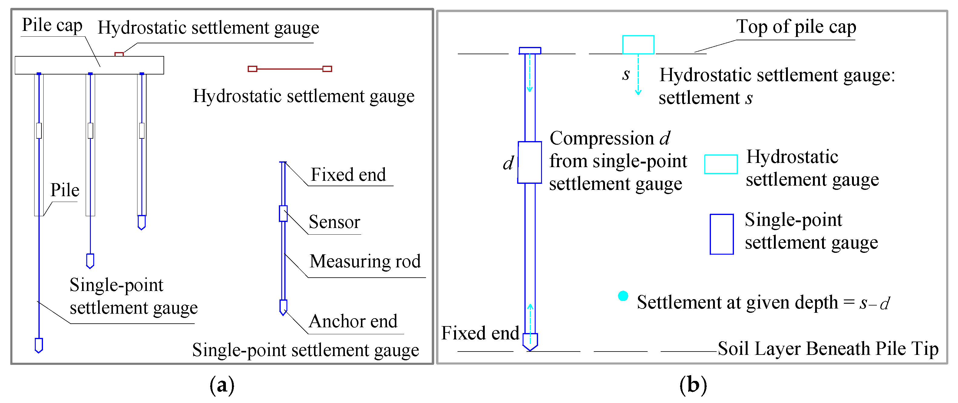
A single-point settlement gauge consists of an anchor, a measuring rod and a sensor. One end is anchored in a pre-designated soil layer and the other at the pile top; the sensor, connected to the rod, measures the total compression from the designated layer to the pile top. Based on electromagnetic induction, a magnetic piston rod fixed to the rod is inserted into a solenoid coil and moves back and forth; the coil inductance varies with the insertion depth. When displacement occurs, the inductance changes, and an inductance-to-frequency conversion circuit converts the change into a frequency signal displayed on a readout unit. A remote automatic monitoring system connected to the gauge achieves automatic data acquisition and transmission.

A hydrostatic settlement gauge consists of a liquid cylinder, a float, a precision level sensor and a protective cover. The measuring point is installed at the top of the pile cap and the reference point on undisturbed ground beyond the influence of the bridge foundation, measuring the settlement of the cap top, i.e., the total compression of the strata. The liquid in the cylinder is kept at the same level through connecting liquid and gas pipes. When the measuring point settles, its float level rises (positive difference), while the reference float level falls (negative difference). Remote automatic monitoring achieves automatic data acquisition and transmission.

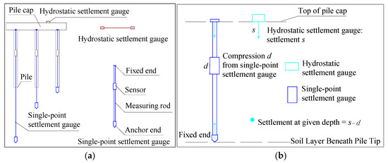
The single-point gauge measures the compression d from a given layer to the pile top, while the hydrostatic gauge measures the total cap settlement s; subtracting the single-point reading from the hydrostatic reading yields the settlement of the strata at a given depth. Single-point gauges are installed at the top and bottom of each target layer, and the difference between two adjacent readings gives the layer compression. The combined measurement principle is shown in Figure 2.

Figure 2. Combined hydrostatic–single-point settlement measurement [10]. (a) Schematic layout of single-point and hydrostatic settlement gauges; (b) schematic diagram of the settlement monitoring principle.

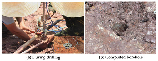
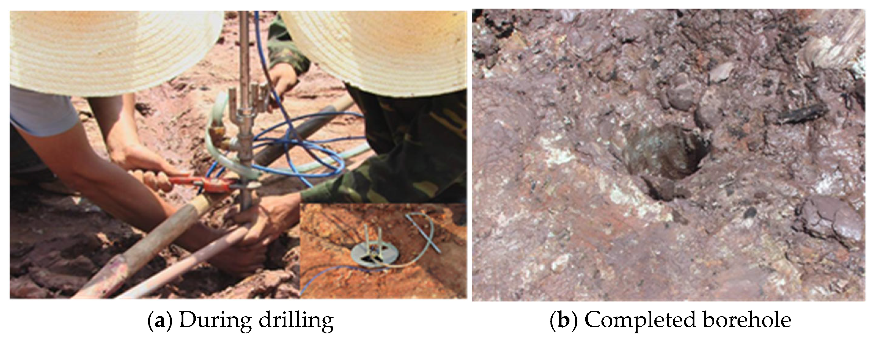
The installation quality of the single-point gauges directly affects measurement accuracy and may even damage the instrument. Pre-drilled boreholes are therefore prepared at selected positions, and the gauges are installed following the procedure shown in Figure 3.

Figure 3. Field installation of single-point settlement gauge.

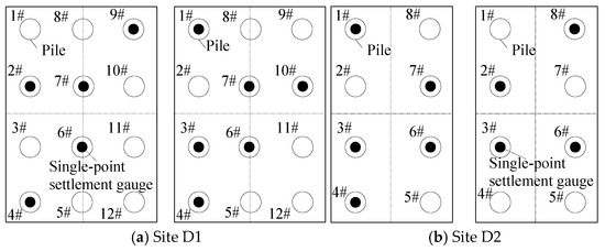
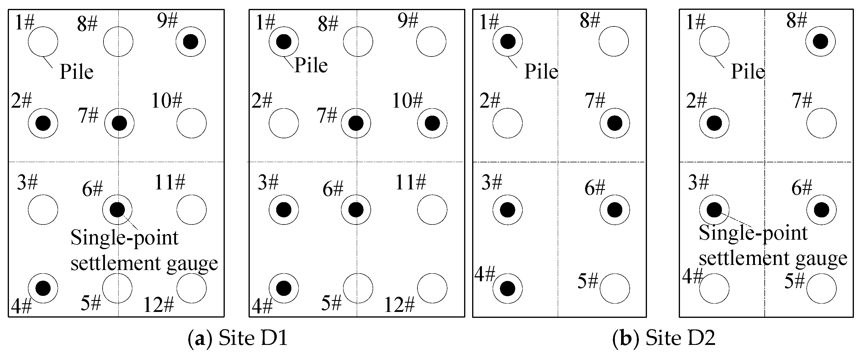
The plan layout of the single-point gauges at sites D1 and D2 is shown in Figure 4, and their installation depths are listed in Table 2, measured from the pile top.

Figure 4. Layout of the single-point settlement gauges. Note: Empty circles are piles; numbers are pile IDs.

Table 2. Embedding depths of single-point settlement gauges.

Site	Depth (m)	Test Site	Depth (m)
D1	52.5	D2	48.5
	54.3		50.5
	55.9		53.6
	56.6		54
	59.0		56.2
	63.0		56.9
	67.9		60.5
	70.5		68.0
	75.1		69.5
	77.3		-
	79.5		-

Both the hydrostatic and single-point gauges have a range of 0–100 mm, a resolution of 0.01 mm and an accuracy of 0.05% FS. The drift value of the settlement gauge is 0.01 mm. Monitoring at sites D1 and D2 commenced in early June 2009, while monitoring at site D3 started in early March 2009. During the monitoring period, construction activities including bridge pier-abutment construction, beam erection, bridge deck work and track laying were carried out sequentially. The loads originate from the self-weight of piers and beams as well as the secondary dead load. Sampling intervals were once daily during construction and weekly during the post-construction rest period; monitoring continued for a further three months after consolidation settlement ceased, giving a total monitoring duration of 16 months. Data were transmitted automatically via GPRS wireless modules.

3.2. Measured Compression Below the Pile Tip

According to the hydrostatic gauge data, the average settlement of the four pile groups at site D1 is 7.1 mm and that of the four at site D2 is 7.2 mm. The hydrostatic settlement comprises the pile shaft compression and the compression of the soil below the pile tip. Following clause 5.5.14 (1) of the Technical code for building pile foundations (JGJ 94–2008, hereafter referred to as the Code) [29], the pile shaft compression is calculated by Equation (1).

$$s_{\mathrm{p}}={\xi }_e{\displaystyle \frac{Ql}{E_c{A}_{ps}}}$$

(1)

where ξ_e is the pile shaft compression coefficient. As these are friction piles, ξ_e is obtained by linear interpolation according to the Code; l is the pile length; Q is the additional load at the pile top under the quasi-permanent load combination, taken as the sum of the superstructure load and the cap self-weight; E_c is the elastic modulus of the pile concrete; and A_ps is the cross-sectional area of the pile. Assuming equal load sharing (see Section 4.3.2), the per-pile top load and the parameters in Equation (1) are given in Table 3. The calculated pile shaft compressions are 1.41 mm and 1.86 mm for D1 and D2, respectively.

Table 3. Calculation of pile shaft compression.

Sites	Q (kN)	L (m)	l/dp	Aps (m2)	ξe	Ec (MPa)	sp (mm)
D1	1758.3	52	41.6	1.23	0.570	3.0 × 104	1.41
D2	1765	48	48	0.79	0.517	3.0 × 104	1.86

The compression of soil beneath pile tips is calculated by Equation (2):

$$s_{\mathrm{s}}^{\ast }=s_{\mathrm{liq}}-s_{\mathrm{p}}$$

(2)

where s_liq is total settlement measured by hydrostatic gauges (mm) and s_p is the pile shaft compression (mm).

Equation (2) gives 5.68 mm and 5.34 mm for D1 and D2, respectively. Based on the single-point gauge data, the layer-wise compressions below the pile tips are listed in Table 4 and Table 5. Summing the layer compressions gives 5.59 mm at D1 and 5.49 mm at D2; the two results agree well, confirming the reliability of the combined monitoring.

Table 4. Compressive deformation of soil (test site D1).

Layer No.	Soil Type	Depth Interval (m)	Layer Thickness (m)	Compression (mm)	Compression per Meter (mm/m)
1	Silty sand, medium dense	52~52.5	0.5	2.86	5.72
2	Silty sand, medium dense	52.5~54.3	1.8	0.63	0.35
3	Silty clay, stiff	54.3~55.9	1.6	0.30	0.188
4	Silty clay, stiff	55.9–56.6	0.7	0.08	0.114
5	Silty clay, firm-to-stiff	56.6~59.0	2.4	0.32	0.133
6	Silty clay, soft	59.0~63.0	4.0	0.92	0.23
7	Silty clay, firm-to-stiff	63.0–67.9	4.9	0.22	0.045
8	Silty sand, dense	67.9–70.5	2.6	0.07	0.027
9	Silty clay, plastic	70.5~75.1	4.6	0.15	0.033
10	Clay, firm-to-stiff	75.1–77.3	2.2	0.02	0.009
11	Silty clay, firm-to-stiff	77.3–79.5	2.2	0.01	0.005

Table 5. Compressive deformation of soil (test site D2).

Layer No.	Soil Type	Depth Interval (m)	Layer Thickness (m)	Compression (mm)	Compression per Meter (mm/m)
1	Clay, firm-to-stiff	48.0–48.5	0.5	4.2	8.40
2	Clay, firm-to-stiff	48.5–50.5	2.0	0.42	0.21
3	Silty clay, stiff	50.5–53.6	3.1	0.38	0.124
4	Silty clay, stiff	53.6–54.0	0.4	0.04	0.10
5	Silty clay, stiff	54.0–56.2	2.2	0.18	0.082
6	Silty clay, stiff	56.2–56.9	0.7	0.05	0.071
7	Silty clay, stiff	56.9–60.5	3.5	0.17	0.049
8	Silty clay, stiff	60.5–68	7.5	0.05	0.007
9	Silty clay, stiff	68–69.5	1.5	0.01	0.007

4. Determination of Additional Stress

The total settlement is calculated by the layer-wise summation method. The compression of each layer is computed and then summed, according to Equations (3) and (4):

$${\mathrm{s}}_{\mathrm{s}}={\displaystyle \frac{1}{E_{s,i}}}{\sigma }_{z,i}\cdot \Delta H_i$$

(3)

$$s_{\mathrm{s}}={\displaystyle \sum _{i=1}^n{s}_{\mathrm{s},i}}$$

(4)

where, E_s,i is the corrected compression modulus of the i-th layer; ΔH_i is the thickness of the i-th layer; σ_z,i is the sum of additional vertical stresses at the mid-thickness of the i-th layer below the pile tip plane, induced by each pile within the horizontal influence range.

4.1. Mindlin–Geddes Solution and Simplification

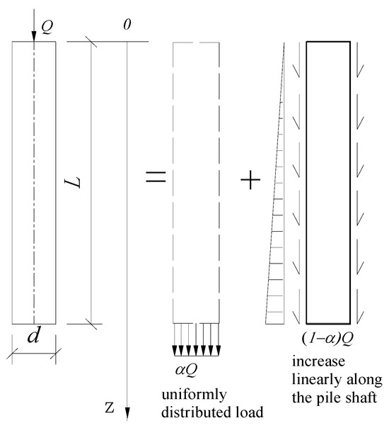
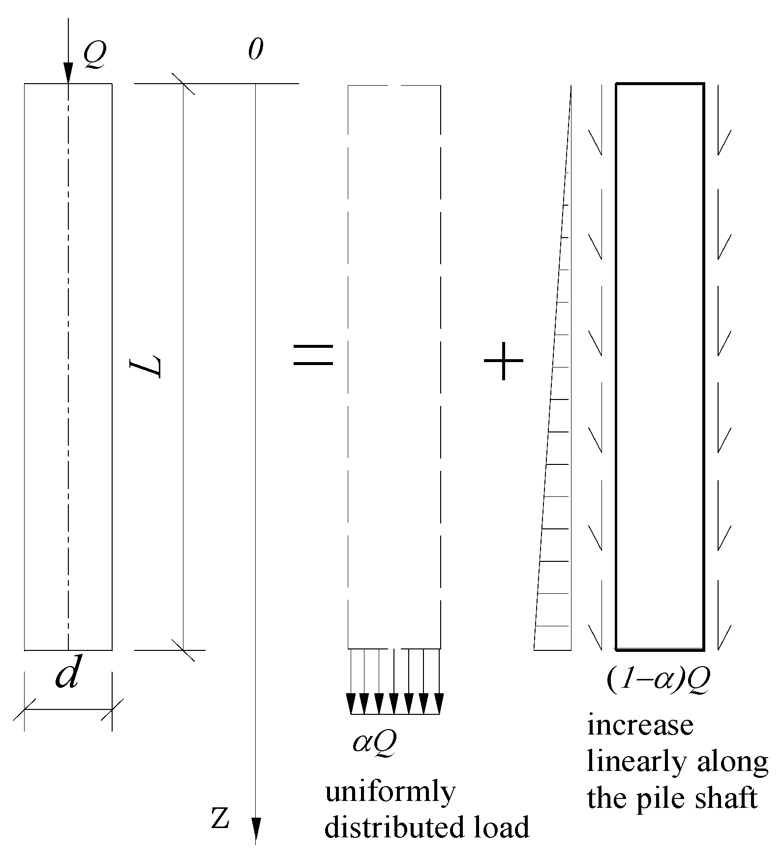
Geddes, Wang and Wang [30,31,32] showed that the additional stress beneath deep-long piles can be obtained from the Mindlin–Geddes analytical solution. This solution extends the Mindlin point-load solution in a semi-infinite elastic medium to the pile–soil system. For a single pile carrying vertical load Q, the total load is decomposed into two parts: (1) tip resistance Q_p = αQ, where α is the tip-resistance ratio and (2) shaft friction Q_s = (1 − α)Q distributed along the pile shaft.

According to Geddes [30], the shaft friction may be assumed uniform or linearly varying (triangular). For bored piles in clay, the triangular distribution (maximum at the pile tip, zero at the surface) is commonly adopted [33]; this better reflects the progressive mobilisation of shaft friction with depth. The strata here are mainly clay or silty clay, so the triangular distribution is used. Based on the Mindlin–Geddes solution, the tip and shaft frictions are simplified as shown in Figure 5.

Figure 5. Load sharing and distribution of tip resistance and shaft friction for a single pile. Note: α is the tip resistance ratio.

Integrating the Mindlin point-load solution over the pile-tip area (tip resistance) and along the pile shaft (shaft friction) gives the vertical stress increment at any point in the soil:

$${\sigma }_z=Q_p{I}_p+Q_s{I}_s$$

(5)

where σ_z is the vertical additional stress; I_p and I_s are the stress influence coefficients for tip resistance and pile shaft friction, respectively, accounting for the pile diameter; Q_p is pile tip resistance, Q_p = αQ; Q_s is pile shaft friction, Q_s = (1 − α)Q, and α is the tip-resistance ratio.

4.2. Calculation of Ip and Is

Geddes, based on Mindlin’s solution for a vertical point load inside an elastic semi-infinite body, equates the tip resistance to a concentrated load at pile-tip depth and the shaft friction to a line load along the pile; line integration of the Mindlin solution yields the influence coefficients. This original solution neglects the actual pile diameter and produces stress singularities near the pile tip. As the present piles are large-diameter, Appendix F of the Code accounts for the pile diameter by double-integration over the circular tip area. According to Appendix F, I_p and I_s are given by Equations (6) and (7).

$$\begin{array}{ll}{I}_p=& {\displaystyle \frac{l^2}{\pi \cdot r^2}}\cdot {\displaystyle \frac{1}{4(1-\nu )}}\left\{2(1-\nu )-{\displaystyle \frac{(1-2\nu )(z-l)}{\sqrt{r^2+{(z-l)}^2}}}-{\displaystyle \frac{(1-2\nu )(z-l)}{z+l}}+{\displaystyle \frac{(1-2\nu )(z-l)}{\sqrt{r^2+{(z+l)}^2}}}\right.-{\displaystyle \frac{{(z-l)}^3}{{\left[r^2+{(z-l)}^2\right]}^{3/2}}}\\ & +{\displaystyle \frac{(3-4\nu )z}{z+l}}-{\displaystyle \frac{(3-4\nu )z{(z+l)}^3}{{\left[r^2+{(z+l)}^2\right]}^{3/2}}}-{\displaystyle \frac{l(5z-l)}{{\left(z+l\right)}^2}}+{\displaystyle \frac{l(5z-l)(z+l)}{{\left[r^2+{(z+l)}^2\right]}^{3/2}}}+{\displaystyle \frac{6lz}{{\left(z+l\right)}^2}}\left.-{\displaystyle \frac{6lz{(z+l)}^3}{{\left[r^2+{\left(z+l\right)}^2\right]}^{5/2}}}\right\}\end{array}$$

(6)

$$\begin{array}{ll}{I}_s=& {\displaystyle \frac{\mathrm{l}}{\pi \cdot r}}\cdot {\displaystyle \frac{1}{4(1-\nu )}}\left\{{\displaystyle \frac{2(2-\nu )r}{\sqrt{r^2+{(z-l)}^2}}}+{\displaystyle \frac{2(1-2\nu )z^2(z+l)-2(2-\nu \left)\right(4z+l)r^2}{lr\sqrt{r^2+{(z+l)}^2}}}\right.\\ & +{\displaystyle \frac{8(2-\nu )z{r}^2-2(1-2\nu )z^3}{lr\sqrt{r^2+z^2}}}+{\displaystyle \frac{12z^7+6z{r}^4(r^2-z^2)}{lr{(r^2+z^2)}^{5/2}}}\\ & +{\displaystyle \frac{15z{r}^4+2(5+2\nu )z^2{(z+l)}^3-4\nu z{r}^4-4z^3{r}^2-r^2{(z+l)}^3}{lr{\left[r^2+{(z+l)}^2\right]}^{3/2}}}\\ & -{\displaystyle \frac{6z{r}^4(r^2-z^2)+12z^2{(z+l)}^5}{lr{\left[r^2+{\left(z+l\right)}^2\right]}^{5/2}}}+{\displaystyle \frac{6z^3{r}^2-2(5+2\nu )z^5-2(7-2\nu )z{r}^4}{lr{\left[r^2+z^2\right]}^{3/2}}}-{\displaystyle \frac{z{r}^3+{(z-l)}^{3}r}{l{\left[r^2+{\left(z-\mathrm{l}\right)}^2\right]}^{3/2}}}\\ & +\left.2(2-\nu ){\displaystyle \frac{r}{l}}\ln {\displaystyle \frac{(\sqrt{r^2+{\left(z-l\right)}^2}+z-l\left)\right(\sqrt{r^2+{\left(z+l\right)}^2}+z+l)}{{\left[\sqrt{r^2+z^2}+z\right]}^2}}\right\}\end{array}$$

(7)

where $\nu$ is Poisson’s ratio of the foundation soil, r is the pile radius, l is the pile length, and z is the vertical distance from the stress calculation point to the pile top. In practice the influence coefficients are obtained from Table F.02 of Appendix F by linear interpolation. As Poisson’s ratio has a negligible effect, $\nu =0.35$ is used throughout.

4.3. Calculation of Additional Stress

For a group of n piles, the total additional stress at any calculation point is obtained by superposition. The vertical additional stress σ_z,_i at the mid-depth of the i-th layer below the j-th pile tip is calculated by Equation (8):

$${\sigma }_{z,\mathrm{i}}={\displaystyle \frac{Q}{l^2}}{\displaystyle \sum _{j=1}^{\mathrm{n}}[\alpha I_{p,j}+(1-\alpha )I_{s,j}]}$$

(8)

where l is the pile length; Q is the vertical load on a single pile, shared by tip resistance and shaft friction; I_p,j and I_s,j are the stress influence coefficients of the j-th pile; and α is the tip-resistance ratio.

4.3.1. Calculation of Tip Resistance Ratio α

According to Article 5.5.14 of the Code, α may be approximated as the ratio of total ultimate tip resistance to the ultimate bearing capacity of a single pile. The ultimate bearing capacity is estimated by empirical relations between soil properties and bearing parameters, using Equations (9) and (10):

$$Q_{uk}=Q_{sk}+Q_{pk}=u{\displaystyle \sum q_{sik}{l}_i}+q_{pk}{A}_p$$

(9)

$$\alpha =Q_{\mathrm{pk}}/Q_{\mathrm{uk}}$$

(10)

where Q_uk is the characteristic ultimate vertical capacity; Q_sk is the characteristic total shaft friction; Q_pk is the characteristic total tip resistance; q_sik is the characteristic ultimate shaft friction of the i-th soil layer, depending on soil properties, consistency and pile type (mud-stabilised bored cast-in-place piles here); and q_pk is the characteristic ultimate tip resistance, which also depends on pile length. Both are obtained from Tables 5.3.5-1 and 5.3.5-2 of the Code; l_i is the thickness of the i-th layer around the pile; u is the pile perimeter; and A_p is the tip area.

For D1, the pile diameter is 1.25 m, the perimeter is 3.925 m and the tip area is 1.227 m²; for D2, the diameter is 1.0 m, the perimeter is 3.14 m and the tip area is 0.785 m². The pile lengths are 52 m and 48 m, respectively. The D1 pile tips lie in dense silty sand and the D2 tips in firm-to-stiff clay. From Table 5.3.5–2, the characteristic ultimate tip resistances are 1200 kPa and 1280 kPa, giving Q_pk1 = 1471.9 kN and Q_pk2 = 1004.8 kN. The characteristic ultimate shaft frictions are listed in Table 6 and Table 7.

Table 6. Characteristic ultimate shaft friction at site D1.

Soil Type	Consistency		Thickness li (m)	qsik (kPa)	Soil	Consistency		Thickness li (m)	qsik (kPa)
Silty clay	Soft	IL = 0.78	1.42	51	Silty clay	Firm	IL = 0.49	2.15	69
Silty clay	Liquid	IL = 1.30	2.2	33	Silty clay	Firm	IL = 0.26	2.35	83
Silty clay	Liquid	IL = 1.33	2.8	32	Silty clay	Plastic	IL = 0.67	2	58
Silty clay	Plastic	IL = 0.68	2.2	57	Silty clay	Firm-to-stiff	IL = 0.39	2	75
Silty clay	Plastic	IL = 0.75	3	53	Silty clay	Soft	IL = 0.82	2.5	49
Silty clay	Firm-to-stiff	IL = 0.48	2	69	Silty clay	Plastic	IL = 0.60	2.4	62
Silty clay	Firm-to-stiff	IL = 0.33	3	79	Silty clay	Plastic	IL = 0.79	1.6	51
Silty clay	Plastic	IL = 0.55	2	65	Silty clay	Firm-to-stiff	IL = 0.30	2.7	81
Silty clay	Soft	IL = 0.80	2	50	Silty clay	Firm-to-stiff	IL = 0.36	2.3	77
Silty clay	Plastic	IL = 0.67	1.25	58	Silty clay	Plastic	IL = 0.62	2	61
Silt	Dense	e = 0.466	1.55	81	Silty clay	Plastic	IL = 0.68	2.5	57
Silty clay	Firm-to-stiff	IL = 0.46	2.2	71	Silty sand	Dense	N = 50	1.88	80

Note: consistency is described from laboratory tests and corresponds to Table 5.3.5-1 of the Code [29]. e is the void ratio, I_L the liquidity index and N the standard penetration blow count. The same applies for subsequent tables.

Table 7. Characteristic ultimate shaft friction at test site D2.

Soil Type	Consistency		Thickness li (m)	qsik (kPa)	Soil	Consistency		Thickness li (m)	qsik (kPa)
Silt	Medium dense	IL = 0.78	1.42	51	Silty clay	Stiff	IL = 0.04	3.9	94
Silty clay	Stiff	e = 0.843	2.83	50	Silt	Dense	e = 0.578	1.4	75
Silty clay	Firm-to-stiff	IL = 0.05	3.5	94	Fine sand	Dense	N = 31	3.5	65
Silt	Dense	IL = 0.29	3.4	81	Silt	Dense	e = 0.591	3.8	75
Silt	Dense	e = 0.646	3.1	70	Silt	Medium Dense	e = 0.780	2.6	58
Fine sand	Medium dense	e = 0.573	3.6	75	Silty clay	Plastic	IL = 0.61	4.5	61
Fine sand	Medium dense	N = 24	2.4	53	Silt	Medium Dense	e = 0.776	3.17	72
Silty clay	Firm-to-stiff	N = 24	2	53	-	-	-	-	-

Substituting the above values into Formulas (9) and (10) gives tip-resistance ratios α = 0.1035 (D1) and α =0.0849 (D2).

4.3.2. Load Assumption for Settlement Calculation

In the pile-shaft compression and additional-stress calculations, all piles within a group are assumed to carry equal load, which is identical to the load adopted for pile-shaft compression: the corresponding values are 1758.3 kN (D1) and 1765 kN (D2).

For a rigid pile cap, owing to pile–soil–pile interaction and cap stiffness, load sharing is non-uniform: corner piles carry the largest load (120–150% of the mean), edge piles an intermediate value (90–110%), and centre piles the least (60–80%) [34,35]. The equal-load assumption is adopted here for the following reasons:

(1) Practical simplification: The main objective is to establish the compression-modulus correction factor β for clay. Single-point gauges at different piles measure the compression of each layer, summed to give the total compression below the pile tip; the equal-load assumption provides a uniform basis for back-calculating the modulus from measured settlement.

(2) Error compensation: In layer-wise summation, the additional stress from the overloaded corner piles partly offsets that from the underloaded centre piles within the compressible strata beneath the cap. Poulos showed that for pile groups at spacing s’ = 3d–6d, the settlement from the equal-load assumption differs from a rigorous non-uniform distribution by generally less than ±15% [34].

(3) Conservative result: The equal-load assumption underestimates the maximum per-pile load (and hence the shaft compression) while slightly overestimating the mean soil additional stress; for settlement prediction this yields a moderately conservative result that satisfies design requirements.

(4) Consistency with the Code: This assumption agrees with the simplified settlement method recommended in the Code [29], where the per-pile load is the total cap load divided by the number of piles.

4.3.3. Additional Stress in the Strata

Equation (8) is used to compute the additional stress in each layer. Layer boundaries follow natural stratification and the gauge measurement range, minimising systematic error; following Design Specifications for Subgrade and Foundation of Highway Bridges and Culverts (hereafter referred to as Code JTG 3363-2019) [36], the layer thickness does not exceed 0.4 times the minimum cap width. The minimum cap side is 9.1 m at D1 (layer thickness ≤ 3.64 m) and 5.0 m at D2 (≤2.0 m). Accordingly, layers 6, 7 and 9 at D1, and layers 3, 5, 7 and 8 at D2, are subdivided. The influence coefficients Ip and Is are obtained by linear interpolation from Table F.02 of Appendix F. The results are given in Table 8 and Table 9.

Table 8. Vertical additional stress at site D1 (l = 52 m, ɑ = 0.104).

Layer	Soil Type	Depth Interval (m)	Layer Thickness $\Delta \mathit{H}$ (m)	Depth zi (m)	α	Ip	Is	Additional Stress (kPa)
1	Silty sand, medium dense	52~52.5	0.5	52.25	0.104	957.157	46.766	91.68
2	Silty sand, medium dense	52.5~54.3	1.8	53.40		247.290	37.388	38.44
3	Silty clay, stiff	54.3~55.9	1.6	55.10		109.099	42.220	31.96
4	Silty clay, stiff	55.9–56.6	0.7	56.25		90.803	25.825	21.17
5	Silty clay, firm-to-stiff	56.6~59.0	2.4	57.80		73.647	21.812	17.67
6-1	Silty clay, soft	59.0~61.5	2.5	60.25		53.025	16.999	13.48
6-2	Silty clay, soft	61.5~63.0	1.5	62.25		41.178	14.183	11.04
7-1	Silty clay, firm-to-stiff	63.0~65.6	2.6	64.30		33.761	12.266	9.42
7-2	Silty clay, firm-to-stiff	65.6–67.9	2.3	66.75		25.416	10.090	7.59
8	Silty sand, dense	67.9–70.5	2.6	69.20		19.969	8.553	6.33
9-1	Silty clay, plastic	70.5~73.0	2.5	71.75		15.851	7.296	5.32
9-2	Silty clay, plastic	73.0~75.1	2.1	74.05		13.098	6.403	4.61
10	Clay, firm-to-stiff	75.1–77.3	2.2	76.20		11.223	5.740	4.10
11	Silty clay, firm-to-stiff	77.3–79.5	2.2	78.40		9.495	5.118	3.62

Note: depths are measured from the pile top. Same for subsequent tables.

Table 9. Vertical additional stress at site D2 (l = 48 m, ɑ = 0.085).

Layer	Soil Type	Depth Interval (m)	Layer Thickness $\mathit{\Delta }\mathit{H}$ (m)	Depth zi (m)	α	Ip	Is	Additional Stress (kPa)
1	Clay, firm-to-stiff	48–48.5	0.5	48.25	0.085	1228.147	43.245	110.19
2	Clay, firm-to-stiff	48.5–50.5	2.00	49.52		212.323	26.853	32.63
3-1	Silty clay, stiff	50.5–52.1	1.60	51.32		91.547	21.205	20.82
3-2	Silty clay, stiff	52.1–53.6	1.50	52.85		65.530	16.964	16.15
4	Silty clay, stiff	53.6–54	0.40	53.8		54.892	14.952	14.05
5-1	Silty clay, stiff	54–55	1.00	54.5		48.872	13.771	12.83
5-2	Silty clay, stiff	55–56.2	1.20	55.6		40.447	12.075	11.10
6	Silty clay, stiff	56.2–56.9	0.70	56.57		34.653	10.859	9.87
7-1	Silty clay, firm-to-stiff	56.9–58.5	1.60	57.72		29.185	9.658	8.67
7-2	Silty clay, stiff	58.5–60.5	2.00	59.5		23.989	8.387	7.44
8-1	Silty clay, stiff	60.5–62	1.50	61.25		19.067	7.182	6.27
8-2	Silty clay, stiff	62–64	2.00	63.0		14.946	6.146	5.28
8-3	Silty clay, stiff	64–66	2.00	65.0		12.510	5.411	4.61
8-4	Silty clay, stiff	66–68	2.00	67.0		9.962	4.658	3.91
9	Silty clay, stiff	68–69.53	1.53	68.77		8.687	4.228	3.53

5. Discussion on Compression Modulus

5.1. Back-Calculated Compression Modulus

From Equation (3), the compression modulus of any layer below the pile tip is calculated by Equation (11):

$$E^{\ast }={\sigma }_{z,\mathrm{i}}\cdot \Delta H_i/s_{s,i}$$

(11)

Substituting the measured layer compression from Table 4 and the additional stresses from Table 8 and Table 9 into Equation (11) gives the average modulus of each layer; subdivided layers are weighted by thickness. The results are listed in Table 10 and Table 11. The piles are bored cast-in-place piles; because the soil at the pile tip is disturbed, the settlement within 0.5 m below the tip is large and does not represent the intact soil. Experience shows that measured values of 3–5 times the instrument resolution may be treated as indicative, while values above 5 times are reliable. Layers 10 and 11 at D1 and layer 9 at D2 have measured values close to the resolution and may reflect measurement noise rather than compression. At D2, layers 8-1 to 8-4 (7.5 m thick) show only 0.05 mm compression, suggesting that the deeper part is virtually uncompressed; treating all of it as compressed also carries uncertainty. These layers are therefore excluded from the β analysis below.

Table 10. Average compression modulus of the strata at site D1.

Layer	Soil Type	Depth Interval (m)	E0 (MPa)	Layer Thickness $\mathit{\Delta }\mathit{H}$ (m)	Compression (m)	Back-Calculated E* (MPa)
1	Silty sand, medium dense	52~52.5	10 *	0.5	2.86	16.03 *
2	Silty sand, medium dense	52.5~54.3	10 *	1.8	0.63	109.82 *
3	Silty clay, stiff	54.3~55.9	10.9	1.6	0.30	170.43
4	Silty clay, stiff	55.9–56.6	10.9	0.7	0.08	185.20
5	Silty clay, firm-to-stiff	56.6~59.0	8.3	2.4	0.32	132.54
6-1	Silty clay, soft	59.0~61.5	4.6	2.5	0.92	48.14
6-2	Silty clay, soft	61.5~63.0	6.9	1.5		75.27
7-1	Silty clay, firm-to-stiff	63.0~65.6	9.5	2.6	0.22	195.99
7-2	Silty clay, firm-to-stiff	65.6–67.9	9.5	2.3		208.12
8	Silty sand, dense	67.9–70.5	12.4 *	2.6	0.07	182.87 *
9-1	Silty clay, plastic	70.5~73.0	7.2	2.5	0.15	157.81
9-2	Silty clay, plastic	73.0~75.1	6.5	2.1		149.3
10	Clay, firm-to-stiff	75.1–77.3	7	2.2	0.02	451.14 *
11	Silty clay, firm-to-stiff	77.3–79.5	7	2.2	0.01	797.00 *

Note: depths are measured from the pile top. The E₀ data for layers 1, 2, and 8 in the table were adopted from the regional experience parameters [37] with a disturbance discount and are subject to uncertainty. Same for subsequent tables. Values marked with * represent uncertain data.

Table 11. Average compression modulus of the strata at site D2.

Layer	Soil Type	Depth Interval (m)	E0 (MPa)	Layer Thickness $\mathit{\Delta }\mathit{H}$ (m)	Compression (m)	Back-Calculated E* (MPa)
1	Clay, firm-to-stiff	48–48.5	6.2	0.5	4.2	13.11
2	Clay, firm-to-stiff	48.5–50.5	6.2	2.03	0.42	157.73
3-1	Silty clay, stiff	50.5–52.1	7.2	1.57	0.38	146.61
3-2	Silty clay, stiff	52.1–53.6	7.2	1.5		154.26
4	Silty clay, stiff	53.6–54	7.2	0.4	0.04	140.52 *
5-1	Silty clay, stiff	54–55	7.2	1	0.18	143.88
5-2	Silty clay, stiff	55–56.2	7.1	1.2		146.64
6	Silty clay, stiff	56.2–56.9	7.1	0.7	0.05	144.05 *
7-1	Silty clay, firm-to-stiff	56.9–58.5	7.1	1.6	0.17	116.89 *
7-2	Silty clay, stiff	58.5–60.5	6.4	2		170.23 *
8-1	Silty clay, stiff	60.5–62	8.1	1.5	0.05	480.98 *
8-2	Silty clay, stiff	62–64	13.5	2		853.06 *
8-3	Silty clay, stiff	64–66	13.5	2		914.06 *
8-4	Silty clay, stiff	66–68	13.5	2		977.43 *
9	Silty clay, stiff	68–69.53	7.7	1.53	0.01	539.95 *

Note: values marked with * represent uncertain data.

5.2. Laboratory Oedometer Test Results of Compression Modulus

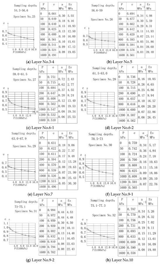
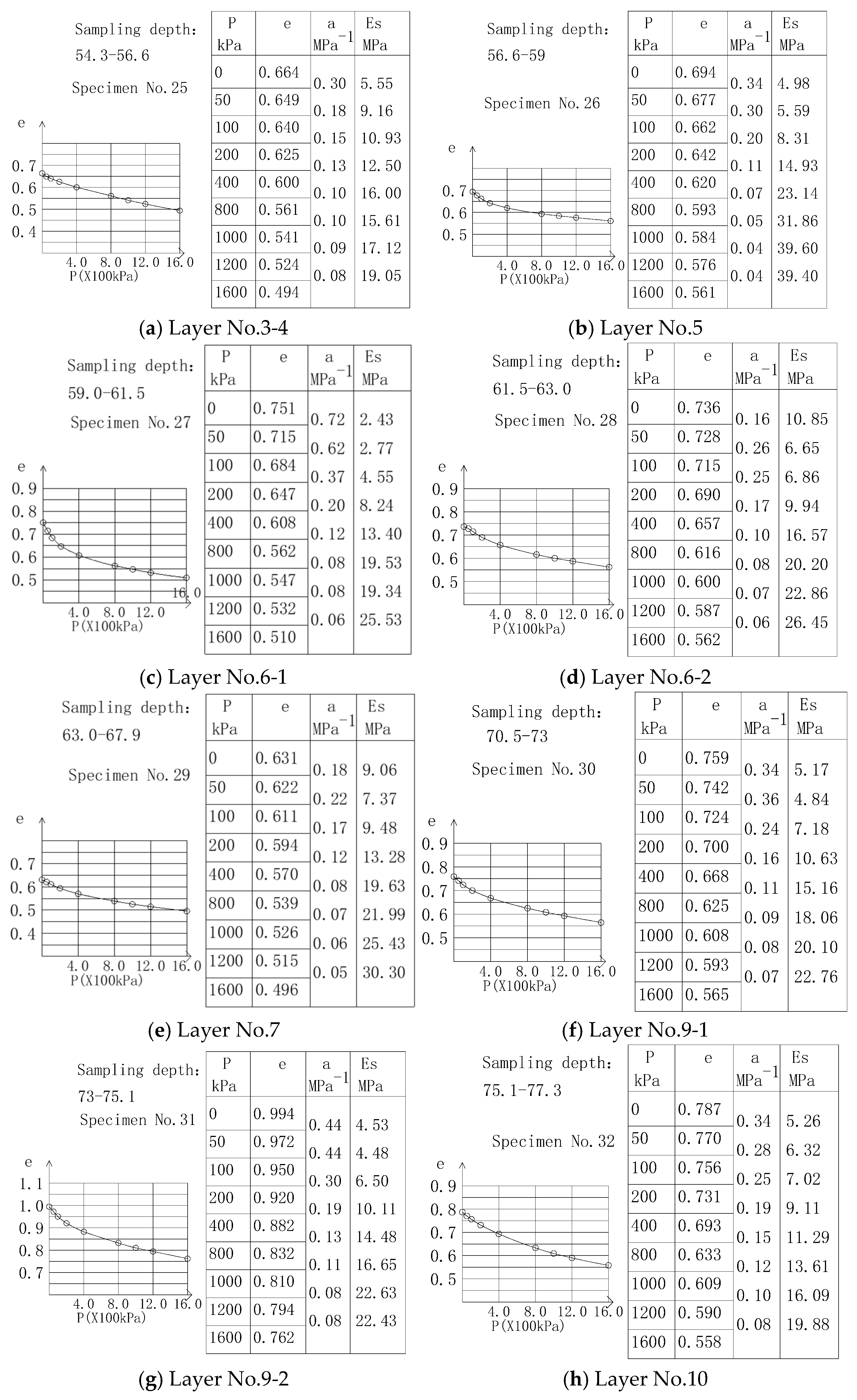
The compression modulus used in settlement calculation is normally obtained from laboratory oedometer tests. Oedometer test results for samples at various depths at D1 is shown in Figure 6. Owing to severe sampling disturbance of the silty sand and fine sand, the compression modulus of undisturbed soil could not be obtained. The E₀ values for layers 1, 2, and 8 in tables were taken as the minimum among the empirical values adopted along the railway line. The geotechnical test data for site D2 are available in the Supplementary Materials.

Figure 6. Oedometer compression modulus of layers 3–7, 9 and 10 at site D1.

At D1, the overburden stress of the soil below the pile tip exceeds 1000 kPa. The compression modulus corresponding to the overburden stress at each sampling point is given as E_w in Table 12. At sampling depths of 54.3–56.6 m, where the geostatic stress is 1100–1200 kPa, E_w/E₀ = 1.57; at depths of 56.6–75.1 m, where the geostatic stress is 1200–1600 kPa, E_w/E₀ = 2.78–5.55. At D2, the overburden stress below the pile tip exceeds 800 kPa; the corresponding E_w values are given in Table 13. At depths of 50.5–56.2 m (geostatic stress 800–1000 kPa), E_w/E₀ = 3.36–3.39; at depths of 56.9–60.5 m (1000–1200 kPa), E_w/E₀ = 3.54–3.76. The increase in compression modulus grows with overburden thickness. The ratio of the back-calculated in-situ modulus to the laboratory value is E*/E₀ = 10.47–22.97, excluding the uncertain values noted above. As Table 12 shows, except for the severely disturbed layer at the pile tip, the E*/E₀ values near the tip exceed those farther away; this is likely because shallow strata below the tip are affected by the additional load from the upper pile, which reduces the void ratio relative to that before pile installation. The actual compression modulus increases with load and varies dynamically, consistent with the understanding that the modulus after pile driving exceeds that before [15]. With increasing depth, the influence of the additional load diminishes; beyond a certain depth, the increase in overburden stress (the in-situ geostatic stress) becomes dominant, so that the E*/E₀ ratio increases. This indicates that the deeper the stratum, the more pronounced the stress release of the specimen, and the more the laboratory modulus is underestimated.

Table 12. Laboratory compression modulus considering geostatic stress at site D1.

Layer	Depth Interval (m)	Depth (m)	Geostatic Stress (kPa)	E0 (MPa)	Ew (MPa)	Ew/E0	E*/E0
3	54.3~55.9	55.12	1173.07	10.9	17.12	1.57	15.64
4	55.9–56.6	56.27	1188.14	10.9	17.12	1.57	16.99
5	56.6~59.0	57.80	1232.99	8.3	39.40	4.75	15.97
6-1	59.0~61.5	60.25	1279.79	4.6	25.53	5.55	10.47
6-2	61.5~63.0	62.25	1325.33	6.9	26.45	3.83	10.91
7-1	63.0~65.6	64.30	1366.33	9.5	26.45	2.78	20.63
7-2	65.6–67.9	66.77	1408.36	9.5	26.45	2.78	21.91
9-1	70.5~73.0	71.75	1498.51	7.2	22.76	3.16	21.92
9-2	73.0~75.1	74.07	1543.63	6.5	22.43	3.45	22.97

Note: calculation depths are measured from the pile top; the depth for overburden stress is the table value + 4.38 m.

Table 13. Laboratory compression modulus considering geostatic stress at site D2.

Layer	Depth Interval (m)	Depth (m)	Geostatic Stress (kPa)	E0 (MPa)	Ew (MPa)	Ew/E0	E*/E0
3-1	50.5–52.1	51.32	894.718	7.2	24.42	3.39	20.36
3-2	52.1–53.6	52.85	925.61	7.2	24.42	3.39	21.43
4	53.6–54	53.8	944.8	7.2	24.42	3.36	19.52
5-1	54–55	54.5	959.29	7.2	24.2	3.36	19.98
5-2	55–56.2	55.6	982.06	7.1	24	3.38	20.65
6	56.2–56.9	56.57	1002.04	7.1	24	3.76	20.29
7-1	56.9–58.5	57.72	1025.50	7.1	26.72	4.18	16.46 *
7-2	58.5–60.5	59.5	1061.91	6.4	31.94	3.54	26.60 *

Note: where a layer was not sampled, the modulus is referenced to a similar nearby stratum; calculation depths are measured from the pile top; the overburden depth is the table value + 3.173 m. Values marked with * represent uncertain data.

5.3. Discussion of the Compression-Modulus Correction

5.3.1. Correction Factor β

The compression modulus is a key index of soil compressibility and is used mainly for settlement calculation in bridge pile design, so its proper selection is essential. Owing to the cost and logistics of field tests, laboratory oedometer tests remain the common method; however, high-pressure tests are rare and most reports give E₀ over 100–200 kPa, which is markedly smaller than the actual modulus of deep soil, leading to overestimated and conservative settlement. A correction is therefore usually required. References [13,16], based on laboratory E₀, propose Equations (12) and (13):

$$E_{\mathrm{s}}=(1.42-1.49)E_0$$

(12)

$$E_{\mathrm{s}}=(0.0039{\sigma }_z+0.47)E_0$$

(13)

The corrected modulus from Equations (12) and (13) is far below the back-calculated modulus, indicating significant regional differences; these coefficients should not be applied directly. Reference [38] offers an alternative, Equation (14):

$$E_{\mathrm{s}}=E_0\left[1+{\left({\displaystyle \frac{z_i}{h_0}}\right)}^{{\beta }^{-1}}\right]$$

(14)

where z is the layer depth (m), h₀ is a reference depth taken as 10 m, and β is related to sample disturbance and effective-stress loss: the less the disturbance and stress loss, and the stiffer the soil, the smaller β. Reference [38] recommends β = 1–2.5 for stiff and firm clay; Equation (13) is based on E₀ and accounts for the depth effect on stress loss, but the value of β requires further regional calibration. Linearising Equation (14) gives Equation (15) for β:

$$\beta ={\displaystyle \frac{\ln (z_{\mathrm{i}}/h_0)}{\ln (E^{\ast }/E_0-1)}}$$

(15)

With h₀ = 10 m, the β values back-calculated from E₀ and E* for each layer are listed in Table 14 and Table 15. As layer 7 at D2 contains two sublayers of different consistency with uncertain back-calculated values, it is excluded from the discussion. At D1, β ranges from 0.625 to 0.798; at D2, from 0.552 to 0.586. The clay here is mainly stiff and firm-to-stiff, with minor amounts of plastic and soft clay; the soft clay gives the largest β, whereas the stiff clay gives the smallest.

Table 14. Correction factor β for the strata at site D1.

Layer No.	Soil Type	IL	Depth (m)	Compression (mm)	E0 (MPa)	E* (MPa)	β	1/β
3	Silty clay, stiff	0.20	54.3–55.9	0.30	10.9	170.43	0.6313	1.584
4	Silty clay, stiff	0.20	55.9–56.6	0.08	10.9	185.2	0.634	1.578
5	Silty clay, firm-to-stiff	0.48	56.6–59.0	0.32	8.3	132.54	0.648	1.542
6-1	Silty clay, soft	0.77	59.0–61.5	0.92	4.6	48.14	0.798	1.253
6-2	Silty clay, soft	0.76	61.5–63.0	0.92	6.9	75.27	0.798	1.253
7-1	Silty clay, firm-to-stiff	0.26	63.0–65.6	0.22	9.5	195.99	0.625	1.6
7-2	Silty clay, firm-to-stiff	0.26	65.6–67.9	0.22	9.5	208.12	0.625	1.6
9-1	Silty clay, plastic	0.52	70.5–73.0	0.15	7.2	157.81	0.648	1.543
9-2	Silty clay, plastic	0.52	73.0–75.1	0.15	6.5	149.30	0.648	1.543

Table 15. Correction factor β for the strata at Site D2.

Layer No.	Soil Type	IL	Depth (m)	Compression (mm)	E0 (MPa)	E* (MPa)	β	1/β
3-1	Silty clay, stiff	0.23	50.5–52.1	0.38	7.2	146.61	0.552	1.812
3-2	Silty clay, stiff	0.23	52.1–53.6	0.38	7.2	154.26	0.552	1.812
4	Silty clay, stiff	0.23	53.6–54.0	0.04	7.2	140.52	0.577	1.735
5-1	Silty clay, stiff	0.23	54.0–55.0	0.18	7.2	143.88	0.576	1.736
5-2	Silty clay, stiff	0.23	55.0–56.2	0.18	7.1	146.64	0.576	1.736
6	Silty clay, stiff	0.23	56.2–56.9	0.05	7.1	144.05	0.586	1.708
7-1	Silty clay, firm-to-stiff	0.26	56.93–58.5	0.16	7.1	116.89	0.640	1.563 *
7-2	Silty clay, stiff	0.23	58.5–60.5		6.4	170.23	0.550	1.818 *

Note: values marked with * represent uncertain data.

Table 14 and Table 15 show that β clusters regionally. The two sites, 115 km apart and both dominated by silty clay and clay, exhibit similar stress-loss and disturbance patterns in deep clay. The β⁻¹ column (the logarithmic term in Equation (15), representing the amplification from laboratory to in-situ modulus) ranges from 1.253 to 1.60 at D1 and 1.71 to 1.81 at D2 (uncertain values excluded), with the smallest values in soft soil. The E*/E₀ ratio is therefore not constant but depends on soil consistency and varies non-linearly with depth.

5.3.2. Sensitivity Analysis

The sensitivity analysis addresses three factors: the β value, non-uniform load distribution and measurement resolution.

(1) Sensitivity to β. After excluding the values flagged as uncertain, the mean β values for stiff, firm-to-stiff, plastic and soft clays are 0.585, 0.633, 0.648 and 0.798, respectively. Using the 15 accepted layer-scale β–I_L pairs gives β = 0.511 + 0.338 I_L (R² = 0.805). Taking these class-mean β values as the baseline, the response of each layer to a ±0.05 change in β is shown in Table 16.

Table 16. Sensitivity of settlement to β (baseline by soil consistency).

Site	Depth (m)	State	Measured (mm)	βbase − 0.05 (mm)	βbase (mm)	βbase + 0.05 (mm)	−0.05%	+0.05%
D1	54.3–55.9	Stiff	0.3	0.186	0.241	0.299	−22.9	+24.1
D1	55.9–56.6	Stiff	0.08	0.052	0.068	0.084	−23.2	+24.5
D1	56.6–59.0	Firm-to-stiff	0.32	0.240	0.301	0.363	−20.2	+20.9
D1	59.0–61.5	Soft	0.7	0.609	0.698	0.787	−12.8	+12.7
D1	61.5–63.0	Soft	0.22	0.192	0.220	0.249	−13.1	+13.0
D1	63.0–65.6	Firm-to-stiff	0.128	0.102	0.129	0.159	−21.4	+22.6
D1	65.6–67.9	Firm-to-stiff	0.092	0.068	0.087	0.107	−21.9	+23.1
D1	70.5–73.0	Plastic	0.086	0.066	0.084	0.104	−21.6	+23.0
D1	73.0–75.1	Plastic	0.064	0.051	0.065	0.080	−22.0	+23.4
D1	Subtotal	Stiff	0.38		0.309		−22.9	+24.2
		Firm-to-stiff	0.54		0.517		−20.8	+21.7
		Soft	0.92		0.919		−12.9	+12.7
		Plastic	0.15		0.149		−21.8	+23.2
	Total	—	1.99	1.565	1.894	2.196	−17.4	+17.9
D2	50.5–53.6	Stiff	0.38	0.352	0.452	0.556	−22.1	+23.1
D2	53.6–54.0	Stiff	0.04	0.032	0.042	0.052	−22.6	+23.7
D2	54.0–56.2	Stiff	0.18	0.145	0.188	0.234	−22.9	+24.1
D2	56.2–56.9	Stiff	0.05	0.037	0.048	0.060	−23.2	+24.6
D2	Total	—	0.650	0.567	0.730	0.902	−22.4	+23.5

Table 16 shows the following:

(i) A decrease of 0.05 in β reduces the calculated total compression by 17.4% at D1 and 22.4% at D2, whereas an increase of 0.05 raises it by 17.9% and 23.5%, respectively. As the layer sensitivity factor is positive, underestimating β always underpredicts settlement and is therefore unsafe. The sensitivity factor generally increases with depth for a given soil consistency and decreases as β increases. For example, at D1 layer 7-2, a ±0.05 change in β produces changes of approximately −21.9%/+23.1% in the calculated compression, while the relative sensitivity of the soft layers is only about −12.8%/+13.0%.

(ii) The layer sensitivity factor increases with depth for a given consistency and decreases with β. The layer sensitivity factor is given by Equation (16):

$$\eta ={\displaystyle \frac{\mathsf{\partial }\mathit{ln}{s}_{s,i}}{\mathsf{\partial }\beta }}=f\cdot {\displaystyle \frac{\mathit{ln}(z_i/10)}{{\beta }^2(1+f)}},\begin{array}{ccc}& & \end{array}f={(z_i/10)}^{{\beta }^{-1}}$$

(16)

η is the semi-elastic coefficient of the calculated compression of layer i with respect to β, representing the relative change in compression caused by a small absolute change in β. For finite perturbations, the exact ratio in Equation (16) should be used. Equation (16) shows that, for a given soil consistency, η increases with depth, whereas at a given depth it decreases as β increases. Consequently, the deeper strata below the pile tip are more sensitive to β misjudgement, while soft clay has a lower relative sensitivity because of its larger β. For example, at D1 layer 7-2, a ±0.05 change in β changes the calculated compression by approximately −21.9%/+23.1%, whereas the corresponding changes in the soft layers are only about −12.8%/+13.0%.

(iii) Among the four consistency classes, the soft and firm-to-stiff classes remain the main contributors to the uncertainty of the calculated total settlement at D1. The updated baseline total settlement is 1.894 mm, of which the stiff, firm-to-stiff, plastic and soft classes contribute 0.309, 0.517, 0.149 and 0.919 mm, respectively, corresponding to 16.3%, 27.3%, 7.9% and 48.5% of the total. When only the soft-class β is changed by ±0.05, the total settlement becomes 1.776 and 2.011 mm, corresponding to −6.2% and +6.2%. The corresponding values for the firm-to-stiff class are 1.787 and 2.066 mm, or −5.7% and +5.9%. By comparison, perturbing the stiff and plastic classes changes the total settlement by only −3.6%/+4.1% and −1.7%/+1.8%, respectively. Thus, the dominant effect of the soft class results from its largest share of the total settlement, even though its layer-scale sensitivity is relatively low. Sampling quality and liquidity-index determination should therefore be prioritised for soft layer 6 and the firm-to-stiff layers.

(2) Effects of gauge drift and instrument resolution on β. As the layer compression is obtained from the difference between two readings, the effect of gauge drift is relatively small and can be neglected. However, the standard uncertainty of layer compression induced by instrument resolution should account for the error propagation associated with the two readings.

i. Resolution-induced standard uncertainty of layer compression

The resolution of a single gauge reading is q = 0.01 mm. If the rounding error of a single reading follows a uniform distribution over the interval [−q/2, q/2], its standard uncertainty is $u_1=q/\sqrt{12}$. The measured compression of layer i is $s_i^{\ast }=d_{i,1}-d_{i,2}$. Therefore, by propagating the uncertainties of the two independent readings, the standard uncertainty of the layer compression is obtained as shown in Equation (17):

$$u_{ser}(s_i^{\ast })=\sqrt{{\mathrm{u}}_1^2+u_2^2}={\displaystyle \frac{q}{\sqrt{6}}}$$

(17)

According to Equation (17), the resolution-induced standard uncertainty of layer compression is 0.00408 mm.

ii. Propagation of resolution to the standard uncertainty of β. The standard uncertainty of β induced by instrument resolution can be derived from Equation (14), as shown in Equation (18).

$${\delta }_{\beta }={\displaystyle \frac{\beta }{\ln (E^{\ast }/E_0)}}(1+{\displaystyle \frac{1}{E^{\ast }/E_0-1}}){\displaystyle \frac{u_{res}(s^{\ast })}{s^{\ast }}}$$

(18)

This equation indicates that the standard uncertainty of β is inversely proportional to the measured layer compression. Consequently, layers with smaller measured compressions are more strongly affected by instrument resolution. The calculated standard uncertainties of β range from 0.0023 to 0.0140 at D1, with the maximum value occurring in layer 9-2, and from 0.0042 to 0.0212 at D2, with the maximum value occurring in layer 4. The resolution effect is generally small for layers with moderate compression, but it increases significantly for layers with small compression. For example, at layer 4 of site D2, although the measured compression is only 0.040 mm, the standard uncertainty of β reaches 3.68% of its back-calculated value. Therefore, the resolution effect should not be neglected for low-compression layers, such as layer 9-2 at D1 and layers 4 and 6 at D2.

(3) Combined uncertainty and recommended values. Based on the above analysis, the recommended combined uncertainty band for β is ±0.06. This value combines the ±0.05 sensitivity associated with soil-consistency classification and model selection with the maximum resolution-induced standard uncertainty of approximately 0.021. Gauge drift is neglected under the assumption that its effects cancel in the difference between the two gauge readings. Extending the band to ±0.06 gives approximately −20.8%/+21.5% at D1 and −26.7%/+28.3% at D2. Recommendations: (i) control the β scatter within ±0.05; (ii) select β by consistency from Table 17, or use β = 0.511 + 0.338 I_L when I_L is measured.

Table 17. Recommended correction factor β for deep clay.

Soil Consistency	IL Range	Recommended β	Basis
Stiff	0–0.25	0.53–0.65	n = 8, mean 0.585
Firm-to-stiff	0.25–0.50	0.57–0.69	n = 3, mean 0.633
Plastic	0.50–0.75	0.59–0.71	n = 2, mean 0.648
Soft	0.75–1.00	0.74–0.86	n = 2, mean 0.798
No data	—	0.57–0.69	Baseline 0.632, conservative

The strata below the pile tip in this project are mainly stiff, with few samples of other consistencies; the sample size should be expanded in future work.

5.4. Validation at an Independent Site

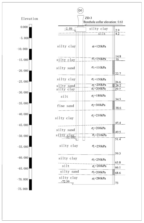
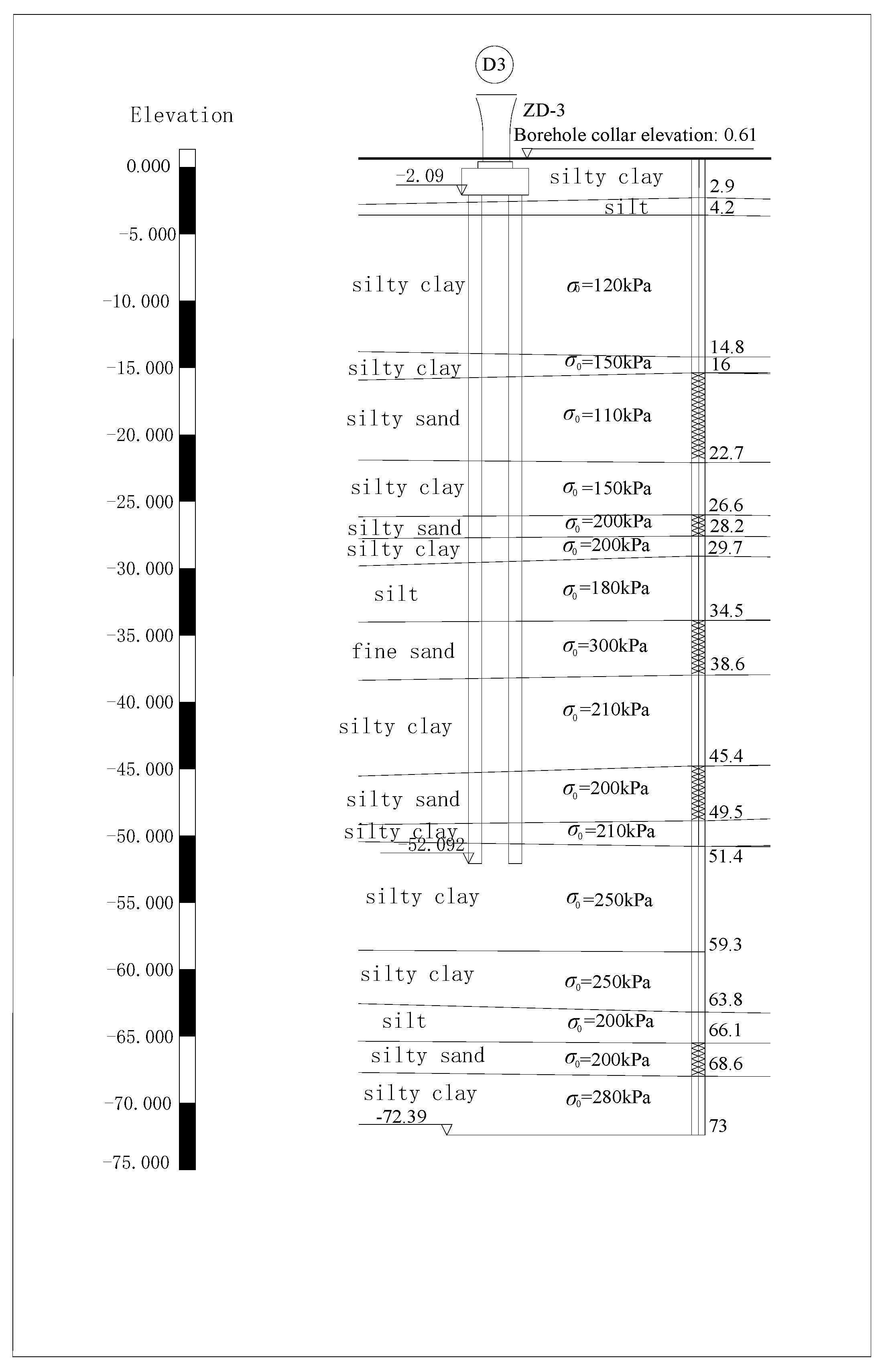
Site D3 in Tianjin is used for validation. This pier lies between D1 and D2, about 28 km from D1. The pile group uses bored piles of 1.00 m diameter and comprises 8 piles of 50 m length; the cap is 10.5 m long and 14.87 m wide, with a total load of 14,720 kN and a mean per-pile load of 1840 kN. The stratigraphy is shown in Figure 7, and the soil parameters below the tip in Table 18. The gauge positions and measured compressions are given in Table 19. The D3 monitoring data were obtained in the same monitoring campaign as D1 and D2 and have not been published previously.

Figure 7. Geological cross-section at site D3.

Table 18. Soil parameters below the pile tip at site D3.

Layer	Soil Type	Interval (m)	Thickness (m)	${\mathit{\gamma }}_{\mathbf{s}}$ (kN/m3)	Poisson’s Ratio $\mathit{\nu }$	E0 (MPa)
1	Silty clay, soft	50.0–50.5	0.5	20.2	0.32	9.2
2	Silty clay, soft	50.5–52.0	1.5	20.2	0.32	9.2
3	Silty clay, stiff	52.0–53.5	1.5	19.9	0.28	10.8
4	Silty clay, stiff	53.5–55.0	1.5	19.9	0.28	10.8
5	Silty clay, plastic	55.0–56.3	1.3	20.4	0.30	7.9
6	Silty clay, plastic	56.3–58.0	1.7	20.4	0.30	7.9
7	Silty clay, firm-to-stiff	58.0–60.0	2.0	20.3	0.29	12.6
8	Silty clay, firm-to-stiff	60.0–60.7	0.7	20.3	0.29	12.6
9	Silt, medium dense	60.7–62.4	1.7	20.4	0.29	12.0
10	Silty sand, dense	62.4–63.7	1.3	19.7	0.28	14.0
11	Silty sand, dense	63.7–65.7	2.0	19.7	0.28	14.0
12	Silty clay, firm-to-stiff	65.7–66.7	1.0	20.4	0.29	17.7
13	Silty clay, firm-to-stiff	66.7–67.6	0.9	20.4	0.29	17.7
14	Silty clay, firm-to-stiff	67.6–68.8	1.2	20.4	0.29	12.4
15	Silty clay, firm-to-stiff	68.8–70.3	1.5	20.4	0.29	12.4

Note: depths are measured from the pile top.

Table 19. Gauge depths and measured compression at site D3.

Depth Below Pile Top (m)	Cumulative Compression (mm)	Layer Thickness (m)	Compression (mm)	Per-Meter Compression (mm/m)
50.0	0	-	-	-
50.5	4.13	0.5	4.13	8.26
55.0	5.15	14.5	1.02	0.070
60.0	5.53	5.0	0.38	0.076
65.69	5.63	5.69	0.10	0.018
70.30	5.64	4.61	0.01	0.002

Using Equations (9) and (10), the tip-resistance ratio is computed. The characteristic ultimate shaft friction is listed in Table 20; summing the values in Table 20 gives a total ultimate shaft friction of 9457.63 kN. The characteristic ultimate tip resistance is 800 kPa, giving a calculated tip resistance of 628 kN. The resulting tip-resistance ratio is 0.063. Following the same layering as in Section 4.3.3, Equation (8) gives the additional stress (Table 21); I_p and I_s are obtained by linear interpolation from Appendix F, Table F.02.

Table 20. Characteristic ultimate shaft friction at site D3.

Soil	Consistency	IL/N	li (m)	qsik (kPa)	Soil	Consistency	IL/N	li (m)	qsik (kPa)
Silty clay	Plastic	IL = 0.56	0.54	64.4	Silty clay	Plastic	IL = 0.71	1.86	55.4
Silt	Medium dense	IL = 1.81	0.96	43.3	Silt	Medium dense	IL = 0.83	2.4	62.0
Silty clay	Plastic	IL = 0.72	2.80	54.8	Silt	Medium dense	IL = 1.01	2.0	57.5
Silty clay	Soft	IL = 0.95	2.0	41.0	Fine sand	Dense	N = 30	4.27	72.0
Silty clay	Plastic	IL = 0.71	5.54	55.4	Fine sand	Soft	IL = 0.91	4.4	43.4
Silty clay	Plastic	IL = 0.59	1.80	62.6	Silty clay	firm-to-stiff	IL = 0.38	3.28	75.68
Silty sand	Medium dense	N = 20	6.21	58.0	Silty clay	Dense	N = 30	1.82	72.0
Silty clay	firm-to-stiff	IL = 0.40	2.0	74.4	Silty sand	Plastic	IL = 0.59	2.8	62.6
Silty clay	Stiff	IL = 0.15	2.13	88.8	Silty clay	Soft	IL = 0.96	1.54	40.4
Silty sand	Medium dense	N = 20	1.63	58.0	-	-	-	-	-

Note: consistency is described from laboratory tests and corresponds to Table 5.3.5-1 of the Code [29]; I_L is the liquidity index and N the standard penetration blow count. Same for subsequent tables.

Table 21. Additional stress at site D3.

Layer	Soil Type	Depth (m)	H (m)	Zi (m)	α	Ip	Is	σz (kPa)
1	Silty clay, soft	50.0–50.5	0.5	50.25	0.063	1313.358	45.200	92.069
2	Silty clay, soft	50.5–52.0	1.5	51.25		295.817	32.786	36.327
3	Silty clay, stiff	52.0–53.5	1.5	52.75		118.520	24.282	22.241
4	Silty clay, stiff	53.5–55.0	1.5	54.25		79.826	19.344	17.042
5	Silty clay, plastic	55.0–56.3	1.3	55.63		61.491	16.081	13.941
6	Silty clay, plastic	56.3–58.0	1.7	57.13		45.355	12.995	11.065
7	Silty clay, firm-to-stiff	58.0–60.0	2.0	59		34.877	10.861	9.108
8	Silty clay, firm-to-stiff	60.0–60.7	0.7	60.34		29.098	9.59	7.963
9	Silt, medium dense	60.7–62.3	1.7	61.53		25.758	8.782	7.251
10	Silty sand, dense	62.3–63.7	1.4	63.03		21.515	7.757	6.347
11	Silty sand, dense	63.7–65.7	2.0	64.69		16.836	6.626	5.350
12	Silty clay, firm-to-stiff	65.7–66.7	1.0	66.19		14.492	5.983	4.798
13	Silty clay, firm-to-stiff	66.7–67.6	0.9	67.14		13.313	5.637	4.505
14	Silty clay, firm-to-stiff	67.6–68.8	1.2	68.20		12.011	5.255	4.181
15	Silty clay, firm-to-stiff	68.8–70.3	1.5	69.55		10.344	4.765	3.766

Note: depths are measured from the pile top.

The per-metre compression of the strata from 65.69 to 70.3 m below the pile top is 0.002 mm, so these layers may be taken as uncompressed; layers 12–14 also change little with depth and may be considered unaffected by the upper load, giving a calculation depth of 15.69 m below the pile tip. For the 0.5 m disturbed zone below the tip, 1.2 E₀ was adopted for the soft clay, following the recommendation in Section 5.5. The remaining layers in Table 18 are corrected by Equation (14), using the maximum and minimum β from Table 17; the results are given in Table 22. The errors between calculated and measured compression between adjacent gauges are 0.96%, −20.8% to 13.3%, −21.2% to 25.6% and −23.7% to 31.3%. The errors for layers 8–11 are relatively large, which is attributed to the excessively wide adopted range of β for layers 9–11 consisting of medium-dense silt and dense silty sand. The calculation results when β takes the base value are shown in Table 23, and the errors between calculated and measured values range from −4.8% to +3.2%, indicating that the recommended β values are suitable for D3.

Table 22. Settlement calculation with an uncertainty band of 0.06 for β at site D3.

Layer	Soil Type	E0 (MPa)	β	Es (MPa)	Depth (m)	Thickness (m)	Calc. Compression (mm)		Error
1	Silty clay, soft	9.2	—	11.15 *	50.0–50.5	0.5	4.17		0.96%
2	Silty clay, soft	9.2	0.74–0.86	70.7–92.9	50.5–52.0	1.5	0.58–0.77	0.81 –0.97	−20.8% ±13.3%
3	Silty clay, stiff	10.8	0.53–0.65	150.3–259.7	52.0–53.5	1.5	0.13–0.22
4	Silty clay, stiff	10.8	0.53–0.65	156.4–273.3	53.5–55.0	1.5	0.09–0.16
5	Silty clay, plastic	7.9	0.59–0.71	96.5–152.7	55.0–56.3	1.3	0.12–0.18	0.30 –0.48	−21.2% ±25.6%
6	Silty clay, plastic	7.9	0.59–0.71	99.9–158.3	56.3–58.0	1.7	0.12–0.19
7	Silty clay, firm-to-stiff	12.6	0.57–0.69	177.6–289.9	58.0–60.0	2.0	0.06–0.10
8	Silty clay, firm-to-stiff	12.6	0.57–0.69	183.1–303.4	60.0–60.7	0.7	0.02–0.03	0.09 –0.16	−23.6% ±31.3%
9	Silt, medium dense	12.0	0.57–0.69	179.0–302.7	60.7–62.4	1.7	0.04–0.07
10	Silty sand, dense	14.0	0.53–0.65	251.8–465.6	62.4–63.7	1.3	0.01–0.03
11	Silty sand, dense	14.0	0.53–0.65	261.5–488.3	63.7–65.7	2.0	0.02–0.04

Note: values marked * are taken as 1.2 E₀.

Table 23. Settlement calculation with base value of β at site D3.

Layer	Soil Type	E0 (MPa)	β	Es (MPa)	Depth (m)	Thickness (m)	Calc. Compression (mm)	Error
1	Silty clay, soft	9.2	_	11.15 *	50.0–50.5	0.5	4.17	0.96%
2	Silty clay, soft	9.2	0.798	80.5	50.5–52.0	1.5	0.68	−4.8%
3	Silty clay, stiff	10.8	0.585	220.1	52.0–53.5	1.5	0.15
4	Silty clay, stiff	10.8	0.585	230.8	53.5–55.0	1.5	0.11
5	Silty clay, plastic	7.9	0.648	119.5	55.0–56.3	1.3	0.15	1.2%
6	Silty clay, plastic	7.9	0.648	124.2	56.3–58.0	1.7	0.15
7	Silty clay, firm-to-stiff	12.6	0.633	220.6	58.0–60.0	2.0	0.08
8	Silty clay, firm-to-stiff	12.6	0.633	228.2	60.0–60.7	0.7	0.02	3.2%
9	Silt, medium dense	12.0	0.633	223.7	60.7–62.4	1.7	0.05
10	Silty sand, dense	14.0	0.585	339.7	62.4–63.7	1.3	0.02
11	Silty sand, dense	14.0	0.585	354.5	63.7–65.7	2.0	0.03

Note: values marked * are taken as 1.2 E₀.

5.5. Recommended Modulus for the Disturbed Zone Below the Pile Tip

In Section 5.1, Section 5.2, Section 5.3 and Section 5.4, the 0.5 m layer immediately below the pile tip was excluded from the back-calculation of β, because boring and pile installation remould this zone and its compression does not represent the intact soil. Nevertheless, the compression of this thin layer dominates the settlement below the tip, contributing 51%, 76% and 73% of the measured totals at D1, D2 and D3, respectively. Its modulus must therefore be assigned explicitly in design rather than by the depth-correction formula of Equation (14).

Applying Equation (11) to the measured compression of this layer at the three sites gives the back-calculated ratios listed in Table 24.

Table 24. Back-calculated modulus of the 0.5 m layer below the pile tip.

Site	Soil Consistency	s* (mm)	σz (kPa)	E* (MPa)	E0 (MPa)	E*/E0
D1	Silty sand, medium dense	2.86	91.68	16.02	10	1.60
D2	Clay, firm-to-stiff	4.20	110.19	13.11	6.2	2.11
D3	Silty clay, soft	4.13	92.07	11.15	9.2	1.21

Note: at D1 the silty sand samples were mostly disturbed, and E₀ = 10.0 MPa was adopted from the regional experience parameters [37] with a disturbance discount.

The back-calculated ratios, ranging from 1.21 to 2.11, are consistent in magnitude with the modulus increase after pile installation reported by Dong et al. [15], and indicate that the disturbed-zone modulus increases with soil stiffness. Two caveats apply: (i) the D1 ratio is based on a referenced E₀ discounted for sampling disturbance rather than site-specific laboratory tests, so it carries the associated uncertainty; (ii) the back-calculated modulus of this zone conflates remolding during construction with the high stress concentration near the tip, so it characterizes the layer response rather than a soil property.

Accordingly, the following design values are recommended for the 0.5 m disturbed zone, obtained by rounding the back-calculated ratios to practical figures: soft clay, 1.2 E₀ (D3:1.21); medium-dense sand, 1.6 E₀ (D1: 1.60, rounded down slightly, which is conservative); and firm-to-stiff clay, 2.0 E₀ (D2: 2.11). These values fall within or marginally above the range reported for sandy soils after pile installation by Dong et al. [15]. Where a single value is required irrespective of soil type, 1.2 E₀ may be adopted for the whole disturbed zone, as it does not exceed any of the three back-calculated values and therefore does not underestimate the compression of this zone; this is conservative, because the disturbed zone dominates the settlement below the tip. For consistency, layer 1 at D3 was computed with 11.15 MPa =1.2 × 9.2 MPa in Table 22 and Table 23, following this recommendation.

As each of the three back-calculated ratios is supported by a single field case, the above values should be regarded as preliminary recommendations pending confirmation at additional monitoring sites.

6. Engineering Application and Recommendations

6.1. Engineering Application

In summary, the correction formula in [38] recommends β= 1–2.5, but the present study shows that the deep clay along this railway is mainly stiff and firm-to-stiff with a little plastic and soft soil; because of differences in soil structure and in-situ stress, β is markedly smaller and closely related to consistency. Combining the fitting and error analyses at D1 and D2, for deep-long pile groups (below 50 m) in this region, β should be selected from Table 17, or computed by β= 0.511 + 0.338 I_L when I_L is measured. In practice: (i) control the β scatter within ±0.05, particularly for soft and firm-to-stiff layers, which contribute most to total settlement; (ii) in the 0.5 m disturbed zone below the tip, take 1.2 E₀ for soft clay, 1.6 E₀ for medium-dense sand and 2.0 E₀ for firm-to-stiff clay.

It should be noted that the study sites lie within the Haihe (North China) Alluvial Plain, where Quaternary deposits are continuous and of similar genesis; this provides a geological basis for extending the correction factor within this unit. However, the measured samples come from only three piers along the Tianjin–Cangzhou section, and the proposed β table should be regarded as preliminary for this geological unit. For other geomorphic units, different depositional origins, or non-cohesive bearing strata, β may deviate significantly and should be re-calibrated by field monitoring.

6.2. Recommendations for Future Research

Based on the analysis of D1 and D2 and the discussion of error sources, to further improve the accuracy of the compression modulus and overcome the limitation of a single linear correction, stress-path-dependent nonlinear models should be developed and combined with in-situ testing, as follows:

(1) Introduce dynamic/nonlinear compression-modulus correction. The compression modulus of deep soil varies dynamically with load, so a single coefficient β (Equation (14)) cannot capture it precisely. A stress-path-dependent dynamic model is recommended, in which the in-situ stress is restored in the laboratory and specimens are loaded in stages along the actual additional-stress path, measuring the intact secant modulus at each stage.

(2) Expand in-situ testing to reduce sampling disturbance. The root cause of the underestimated E₀ is stress release and mechanical disturbance during drilling and sampling; the variation of β (0.53–0.86) with consistency reflects differing disturbance levels. Dilatometer (DMT) or self-boring pressuremeter (SBPM) tests are recommended in deep boreholes to directly measure the in-situ modulus and establish multivariate relations with laboratory E_s, reducing uncertainty at the source.

(3) Establish a regional β database. With only two sites (D1, D2), the β–I_L regression is preliminary. Expanding the sample across depth, plasticity index and liquidity index through long-term monitoring and back-analysis would form a “North China deep-clay β lookup table,” promoting settlement calculation from case-by-case correction to regional standardisation.

7. Conclusions

Using the soil compressions obtained from field tests, this study back-calculated the compression modulus, compared it with laboratory results and existing corrections, and validated the depth-correction formula of [38] by consistency class. The main conclusions are as follows:

(1) The compression modulus exhibits clear regional characteristics. For the deep clay along this railway, the in-situ modulus back-calculated from field tests is 10.47–22.97 times the laboratory E₀ (excluding the disturbed zone below the tip) and varies with depth and consistency; the laboratory value is systematically underestimated and must be corrected before use.

(2) The correction factor β is quantitatively related to soil consistency. Mean β values of 0.585, 0.633, 0.648 and 0.798 are obtained for stiff, firm-to-stiff, plastic and soft clays, with β = 0.511 + 0.338 I_L; the softer the soil, the larger β. With the Mindlin–Geddes additional stress and consistency-based β, the layer-wise settlement agrees with measurements to within −4.8% at D1 and +12.3% at D2.

(3) The correction factor β has a marked effect on settlement and must be strictly controlled. Recommended values are 0.53–0.65 (stiff), 0.57–0.69 (firm-to-stiff), 0.59–0.71 (plastic) and 0.74–0.86 (soft); where no consistency data exist, use 0.57–0.69. In the 0.5 m disturbed zone below the tip, take 1.2 E₀ for soft clay, 1.6 E₀ for medium-dense sand and 2.0 E₀ for firm-to-stiff clay; where a single value is required, 1.2 E₀ may be used for the whole zone. Non-uniform load distribution and instrument resolution introduce an additional β uncertainty of about ±0.06.

(4) The compression modulus is a key parameter for settlement prediction. Future work should (i) develop stress-path-dependent dynamic modulus models to overcome the limitation of single-coefficient linear correction; (ii) promote in-situ tests such as DMT and self-boring pressuremeter tests to eliminate sampling disturbance at the source; and (iii) build a regional β database covering Haihe Alluvial Plain to move settlement calculation from case-by-case correction to regional standardisation.

References

- Wang, W.; Wang, A.; Wu, J.; Hang, Y. Study on settlement computation method for pile foundation by considering pile group reinforcing effect. J. Build. Struct. 2016, 06, 212–218. [Google Scholar] [CrossRef]
- Tian, W.; Ma, J. Research on Calculation Method of Bridge Pile Foundation Settlement of High-speed Railway in Cohesive Soil Area. Railw. Stand. Des. 2013, 4, 55–59. [Google Scholar] [CrossRef]
- Hu, Z.; Ma, J.; Su, C.; Zhou, J. Novel Settlement Prediction Model for Founding High-speed Railway Bridge Piles. J. Saf. Environ. 2015, 15, 93–96. [Google Scholar] [CrossRef]
- Lü, Y.; Liu, H.; Wang, X.; Ding, X.; Zheng, C. Modified Geddes Stress Solution for Calculation of Foundation Additional Stress and Pile Foundation Settlement. J. Sichuan Univ. 2013, 45, 68–74. [Google Scholar] [CrossRef]
- Yang, G.; Yao, L.; Jiang, Y.; Huang, Z. Practical Method for Calculating Nonlinear Settlement of Soft Ground Based on e–p Curve. Chin. J. Geotech. Eng. 2015, 37, 242–249. [Google Scholar] [CrossRef]
- Yang, G.; Li, J.; Jia, K.; Li, Z. Improved Settlement Calculation Method for Engineering Practice. Chin. J. Rock Mech. Eng. 2017, 36, 4229–4234. [Google Scholar] [CrossRef]
- Ning, W. Discussion on Determination of Thickness of Compressed Layer Based on Settlement Estimation of Group-piled Foundation. Explor. Eng. (Rock Soil Drill. Tunn.) 2008, 8, 44–46. [Google Scholar]
- Cheng, Q. Compression Thickness Under Long Piles of High Speed Rail-Way Bridge. Master’s Thesis, Southwest Jiaotong University, Chengdu, China, 2012. [Google Scholar]
- Su, C.; Ma, J.; Pan, H. Field Monitoring and Analysis of Settlement of Super-Long Pile Groups in Deep Soft Soil of Tianjin Extra-Large Bridge on Beijing-Shanghai High-Speed Railway. Railw. Constr. 2013, 8, 16–19. [Google Scholar] [CrossRef]
- Ma, J.; Aziz, H.Y.; Su, C.; Shi, C. Settlement Prediction and Behaviour of Pile Foundations in Deep Clayey Soil Deposits. J. Cent. South Univ. 2014, 21, 1554–1564. [Google Scholar] [CrossRef] [Scilit]
- Luo, S. Selection of Compression Modulus Es for Calculation of Final Foundation Settlement. Geotech. Investig. Surv. 1996, 6, 20–22. [Google Scholar]
- Du, Z.; Li, J. Discussion on formula of modulus of compressibility of soil. J. Changchun Inst. Technol. (Nat. Sci. Ed.) 2003, 4, 30–32. [Google Scholar]
- Chen, X.; Gan, D. Determination of Compression Modulus Es for Soft Soil Foundation. Geotech. Investig. Surv. 1999, 6, 16–18. [Google Scholar]
- Dong, B.; Gan, D. Value Determination Problem of Compression Modulus Es of Soil Layers ⑦, ⑧ and ⑨ in Shanghai Soft Soil Foundation. Hydrogeol. Eng. Geol. 2003, 4, 59–62. [Google Scholar] [CrossRef]
- Dong, B.; Li, Y.; Chen, G.; Gan, D. Comparison Test Study on the Ps of Soft Foundation before and after Pile Insert. Hydrogeol. Eng. Geol. 2003, 1, 33–39. [Google Scholar] [CrossRef]
- Chen, R. Study on Behavior of Pile-Raft Foundation in Soft Soil and Its Design Method. Ph.D. Thesis, Zhejiang University, Hangzhou, China, 2001. [Google Scholar]
- Yu, X.; Cheng, H. Estimation Method and Parameter Optimization of Soil Deformation Modulus. Water Resour. Plan. Des. 2026, 7, 159–163. [Google Scholar] [CrossRef]
- Zhou, C.; Lin, C.; Lin, L.; Yang, X. Research on Dynamic Evolution Law of Compression Modulus of Soft Clay under External Loads. Rock Soil Mech. 2010, 31, 2040–2044. [Google Scholar] [CrossRef]
- Wang, Y. Research on the Prediction of Compression Modulus for High-Pressure Zones in Deep Soil Layers. J. Railw. Eng. Soc. 2021, 38, 41–46. [Google Scholar]
- Skempton, A.W. The pore-pressure coefficients A and B. Géotechnique 1954, 4, 143–147. [Google Scholar] [CrossRef] [Scilit]
- Gorshden, M.H. Geotechnical Problems; Zhang, W., Translator; Geological Publishing House: Beijing, China, 1959; Volume 2. [Google Scholar]
- Li, T.; Qian, S. Evaluation of Soil Sample Disturbance and Determination of Its Preconsolidation Pressure. Chin. J. Geotech. Eng. 1987, 9, 21–30. [Google Scholar]
- Ladd, C.C.; DeGroot, D.J. Recommended practice for soft ground site characterization: Arthur Casagrande Lecture. In Proceedings of Soil and Rock America 2003; MIT: Cambridge, MA, USA, 2003. [Google Scholar]
- Burland, J.B. ‘Small is beautiful’—The stiffness of soils at small strains: Ninth Laurits Bjerrum Memorial Lecture. Can. Geotech. J. 1989, 26, 499–516. [Google Scholar] [CrossRef] [Scilit]
- Hardin, B.O.; Richart, F.E. Elastic wave velocities in granular soils. J. Soil Mech. Found. Div. 1963, 89, 33–65. [Google Scholar] [CrossRef] [Scilit]
- Mayne, P.W.; Kulhawy, F.H. K0–OCR relationships in soil. J. Geotech. Eng. Div. 1982, 108, 851–872. [Google Scholar] [CrossRef] [Scilit]
- Randolph, M.F.; Wroth, C.P. Analysis of deformation of vertically loaded piles. J. Geotech. Eng. Div. 1978, 104, 1465–1488. [Google Scholar] [CrossRef] [Scilit]
- Poulos, H.G. Pile behaviour—Theory and application. Géotechnique 1989, 39, 365–415. [Google Scholar] [CrossRef] [Scilit]
- JGJ 94-2008; Technical Code for Building Pile Foundations. China Architecture & Building Press: Beijing, China, 2008.
- Geddes, J.D. Stresses in foundation soils due to vertical subsurface load. Géotechnique 1966, 16, 231–255. [Google Scholar] [CrossRef] [Scilit]
- Wang, H.; Lin, B.; Zhang, H. Discussion on Mindlin Solution for Pile Foundation Settlement Calculation. Build. Struct. 2018, 48, 806–810. [Google Scholar] [CrossRef]
- Wang, H. Analytical Solution for Pile Settlement Calculation Based on Mindlin and Geddes Stress Solutions. Ind. Constr. 2023, 53, 498–503. [Google Scholar]
- Wang, J.; Wu, G.; Pan, Y.; Jiang, Y.; He, L. Calculation of basal settlement in self-balanced pile tests based on an improved Mindlin solution. J. Undergr. Space Eng. 2019, 15, 92–99. [Google Scholar]
- Poulos, H.G.; Davis, E.H. Pile Foundation Analysis and Design; John Wiley & Sons: New York, NY, USA, 1980. [Google Scholar]
- Randolph, M.F. Design methods for pile groups and piled rafts. In Proceedings of the 13th International Conference on Soil Mechanics and Foundation Engineering; Oxford & IBH: New Delhi, India, 1994; pp. 61–82. [Google Scholar]
- JTG 3363-2019; Design Specifications for Subgrade and Foundation of Highway Bridges and Culverts. China Communications Press: Beijing, China, 2019.
- Pei, Y.; Wang, G. Engineering geological characteristics of Late Quaternary sediments in the southern coastal area of Tianjin Binhai New Area. Geol. Surv. Res. 2016, 3, 215–220. [Google Scholar]
- Chen, F.; Ma, J.; Zhu, L.; Yue, D. Settlement Calculation of Pile Foundation in Deep-soft Soil Considering Depth Effect of Compression Modulus. Rock Soil Mech. 2012, 33, 167–172. [Google Scholar] [CrossRef]
Disclaimer/Publisher’s Note: The statements, opinions and data contained in all publications are solely those of the individual author(s) and contributor(s) and not of MDPI and/or the editor(s). MDPI and/or the editor(s) disclaim responsibility for any injury to people or property resulting from any ideas, methods, instructions or products referred to in the content. |
© 2026 by the authors. Licensee MDPI, Basel, Switzerland. This article is an open access article distributed under the terms and conditions of the Creative Commons Attribution (CC BY) license.