


Abstract
Double-skin façades (DSFs) can moderate heat transfer and airflow between the outdoor environment and the building interior; however, their performance in hot-arid climates is highly dependent on cavity geometry, ventilation arrangement, and the interaction between the airflow and any active cooling surfaces. The objective of this study is to establish, under a single idealised extreme hot-arid design point, how sealed, ventilated and actively cooled double-skin façade cavities differ in their predicted temperature, velocity and turbulent kinetic energy fields, and which arrangements merit controlled follow-up study. The four configurations are treated as an idealised comparative case study rather than as validated building-performance predictions. This exploratory study uses computational fluid dynamics (CFD) to compare the aerothermal behaviour of four DSF cavity configurations under prescribed external air and outer-wall temperatures of 50 °C, an inner-wall temperature of 24 °C, and an external inlet velocity of 3.06 m/s. The configurations comprise a sealed 0.4 m cavity (M1), a wind-driven ventilated 0.4 m cavity (M2), the same ventilated cavity with six 25 mm cooling pipes at 10 °C (M3), and a concept-stage lateral-flow arrangement combining a 0.10 m cavity, a 0.025 m slit and four 80 mm cooling pipes at 10 °C (M4). The simulations employ the standard k-ε turbulence model with fixed thermal boundary conditions. Along the reported sampling lines, M1 exhibited a nearly uniform air temperature of approximately 45.7 °C, whereas M2 remained close to the imposed 50 °C external-air temperature. M3 produced lower temperatures in the immediate vicinity of the cooling pipes, but most of the sampled profile remained near ambient conditions. M4 exhibited a broader spanwise temperature range of approximately 26.9–50 °C, with local pipe-adjacent air temperatures approaching 24 °C and cooler regions developing along parts of the lateral flow path. The findings provide preliminary concept-screening evidence and support further controlled parametric analysis, higher-fidelity modelling, and experimental validation.
1. Introduction
1.1. DSF Concepts and Climate-Dependent Performance
Double-skin façades (DSFs) are multi-layer envelope systems in which an outer skin, an inner skin, and an intermediate cavity work together to moderate heat, airflow, solar gain and acoustic exposure [1,2]. Depending on the design intent, the cavity may be sealed, naturally ventilated, mechanically ventilated, or hybrid-ventilated, and may additionally contain shading, thermal storage, or active heat-exchange components. Reviews of DSF systems consistently emphasise that their performance is not inherent to the typology itself; it depends on climate, orientation, cavity width, opening configuration, glazing/shading specification, control strategy and the interaction with the building services system [3,4,5,6,7,8].
Much of the early DSF literature was generated in temperate or cold European contexts, where the cavity can operate as a solar buffer and reduce winter heat loss. In cooling-dominated climates, however, the same buffering mechanism can become a liability if the cavity traps solar and ambient heat. Systematic reviews therefore caution that a DSF may save energy only when its ventilation and shading strategy is matched to the climate and operating mode; otherwise, overheating, higher cooling loads, maintenance complexity, and uncertain operational control can offset the expected benefits [4,5,6,7,8].
1.2. Hot-Climate Applications and Design Limitations
Evidence from hot-arid and hot-humid settings indicates that DSF design priorities differ from those in heating-dominated climates. Hamza [1] emphasised heat removal in hot-arid applications, while Wong et al. [9] examined an alternative configuration for hot-humid conditions where conventional ventilation can be less effective. For the United Arab Emirates, Aldawoud et al. [10] reported that simulated annual cooling outcomes varied with ventilation mode, cavity width and construction assumptions.
Recent hot-climate reviews and optimisation studies reinforce this climate sensitivity. Abtar [11] identified the Middle East as a challenging application context because high solar gains, dust, maintenance requirements and long cooling seasons alter the feasibility of DSFs. Wang et al. [12] and Naddaf et al. [13] similarly showed that DSF energy performance is controlled by the combined selection of cavity geometry, opening ratios, orientation and operational strategy. These studies support the premise that a DSF intended for Gulf summer conditions must be evaluated as a coupled thermo-fluid system [14] rather than as a generic façade typology.
1.3. CFD Modelling, Ventilation Physics and Boundary-Condition Sensitivity
Numerical modelling has been central to DSF research because the cavity contains coupled conduction, convection, radiation and sometimes buoyancy/wind-driven flow. Early and widely cited modelling studies established the value of thermal network, zonal and CFD methods for predicting cavity temperatures and airflow [15,16,17,18]. Subsequent CFD investigations highlighted that model choices such as turbulence closure, radiation treatment, wall functions, mesh resolution and boundary conditions can materially affect predictions of temperature and velocity in ventilated façade cavities [19,20,21,22,23,24].
Recent reviews of DSF CFD practice argue that validation should include both thermal and kinematic variables because matching temperature alone can hide errors in the velocity field and, therefore, in convective heat transfer [23]. Boundary-condition sensitivity is particularly relevant for hot-climate simulations: Ahmadi et al. [24] showed that airflow and heat-transfer predictions change with the way external and internal boundary conditions are represented, while Catto Lucchino et al. [25] demonstrated that whole-building simulation tools require careful validation when modelling DSFs. These findings justify the present study’s focus on temperature, velocity, and turbulent kinetic energy (TKE) rather than temperature only.
1.4. Active and Hybrid Cavity-Cooling Strategies
Where passive ventilation is insufficient, researchers have explored active or hybrid thermal-control strategies within façade cavities. Water-spray window systems can reduce glass surface temperatures through evaporative cooling, but their applicability in arid regions is constrained by water availability, water quality and maintenance requirements [26]. Shen and Li [27] investigated a DSF with cooling pipes embedded in venetian blinds and showed that direct water-based heat extraction could reduce cavity temperature and inward heat flux, indicating the potential of integrating hydronic cooling surfaces into the cavity. In building energy terms, active cavity cooling of this kind shifts part of the façade cooling duty from the primary HVAC system to a dedicated hydronic circuit, intercepting solar and conductive heat gains at the envelope before they reach the occupied space and thereby lowering the peak cooling load; its net benefit nevertheless depends on the chilled-water supply temperature, pumping energy and condensation control, which lie outside the scope of the present field-level study [10,11,28].
Other studies have used thermal mass or phase-change materials to moderate DSF heat gain. De Gracia et al. [29] assessed ventilated DSFs with phase-change material under different climates, while Li et al. [30,31] developed integrated DSF/PCM blind models to study heat-transfer mechanisms and design parameters. These studies suggest that the effectiveness of a thermal sink can depend on airflow distribution, exposed surface area and the time available for heat exchange; those quantities require direct evaluation rather than inference from temperature contours alone.
1.5. Research Questions and Scope
Although recent hot-climate studies have optimised double-skin façade energy performance through cavity geometry, opening ratios, orientation and operational strategy [8,11,12,13], they have generally not provided a controlled side-by-side comparison of sealed, ventilated and actively cooled cavity concepts under a single extreme hot-arid design point at the level of the resolved temperature, velocity and turbulence fields. The present study addresses this narrower gap through an exploratory, field-level comparison rather than a building-scale energy ranking. This study focuses on three questions relevant to an idealised extreme hot-arid design point. First, how do the predicted temperature, velocity and TKE fields differ among sealed, ventilated and actively cooled cavity concepts when the same prescribed external values are applied? Second, are lower temperatures confined to the vicinity of the cooled surfaces or visible over broader portions of the selected planes and lines? Third, do the reported TKE patterns vary consistently with the sampled temperature fields? These questions are exploratory and are addressed at the level of predicted fields rather than through a comprehensive building-level performance ranking. Among the four configurations, Model 4 is the primary proposed concept, whereas Models 1 to 3 provide the sealed, ventilated and actively cooled reference cases against which it is assessed.
Accordingly, this study presents an exploratory CFD comparison of four DSF cavity configurations, ranging from a sealed baseline to wind-driven ventilated and isothermally cooled concepts. Model 4 is included as a concept study rather than a direct one-to-one comparator because it changes several geometric and cooling variables simultaneously. The analysis uses selected line profiles and contour planes to describe predicted cavity air temperature, velocity magnitude and TKE. It does not quantify whole-cavity heat removal, façade heat flux, HVAC load or net energy performance.
2. Materials and Methods
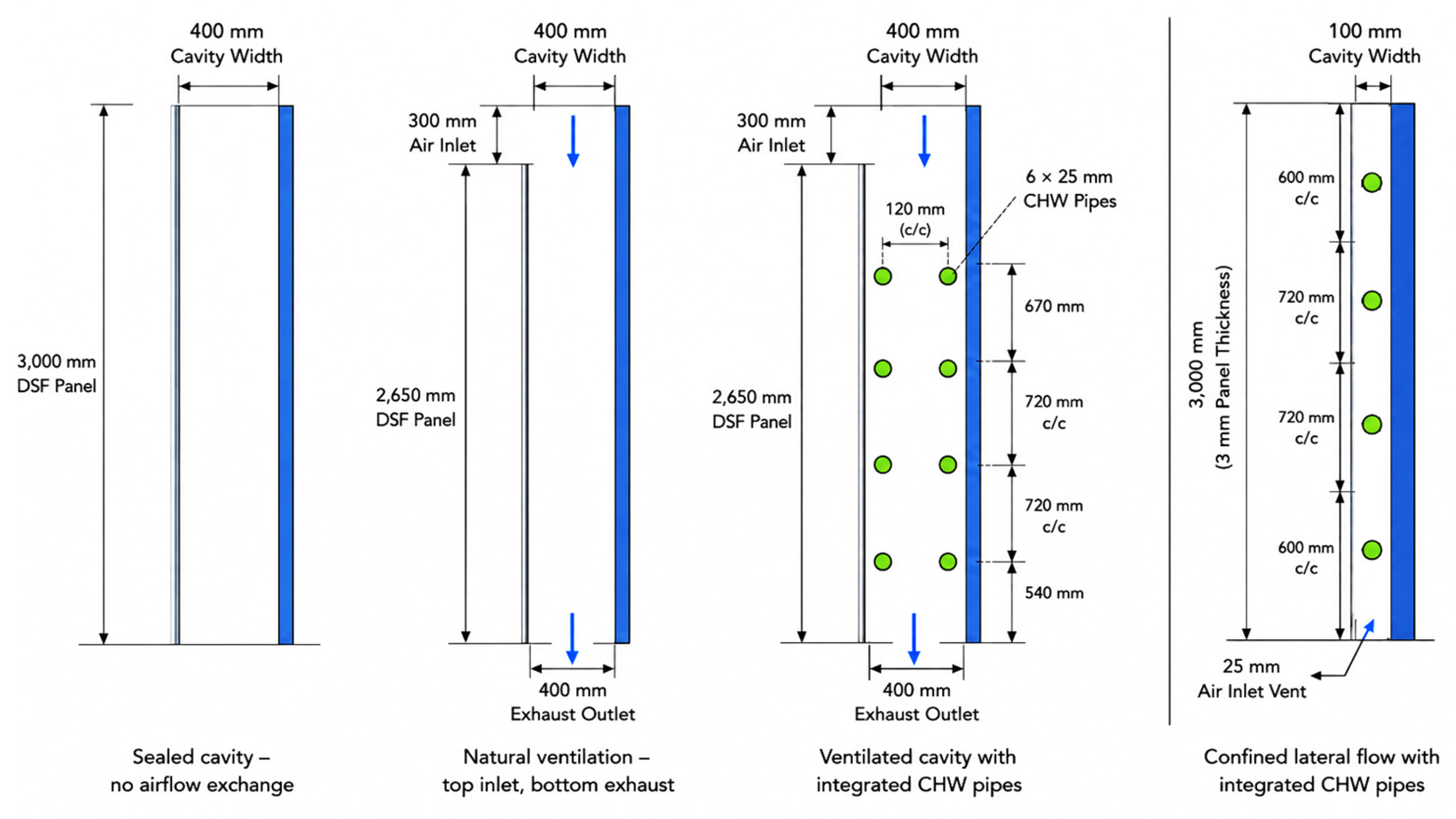
The study compares four DSF configurations (Figure 1) using a common CFD workflow and prescribed 50 °C external conditions. Model 4 is treated as a multivariable concept that combines a narrower cavity, lateral wind-driven flow, different inlet geometry, larger pipes and a different cooling-surface arrangement. The four configurations were selected to form a deliberate progression rather than four unrelated cases: M1 establishes the sealed baseline, M2 isolates the effect of ventilation, M3 adds cooling pipes to the ventilated cavity, and M4 represents the full proposed lateral-flow concept. Models 1 to 3 therefore serve as supporting reference cases that make it possible to separate the effects of ventilation, cooling, and geometry; without them, M4 would have no baseline against which its predicted fields could be interpreted. The aim is to describe the resulting temperature, velocity and TKE patterns and to identify hypotheses for later controlled studies. Residence time, cavity-volume averages, mass-flow rate, pressure drop and heat-transfer rate were not calculated, so causal attribution to geometric confinement or contact time is not attempted.
Figure 1.
Comparative CFD framework for four double-skin façade cavity configurations under common prescribed external and thermal boundary values.
2.1. Computational Framework and Software
All numerical simulations were conducted using ANSYS 2025 R1, utilising ANSYS DesignModeler for geometry creation, the ANSYS Meshing utility for grid generation, ANSYS Fluent 2025 for computational fluid dynamics (CFD) analysis, and ANSYS CFD Post for result visualisation and data extraction. The simulations were performed to investigate airflow and thermal behaviour within double-skin façade (DSF) cavity configurations under controlled and consistent environmental conditions.
ANSYS Fluent was selected as the simulation platform because it is a well-established finite-volume CFD solver that has been extensively applied and validated for double-skin façade and ventilated-cavity studies, including several of the works reviewed in Section 1 [20,21]. Adopting the same solver family used in this body of literature keeps the present results methodologically comparable with prior DSF CFD work. Fluent also provides the coupled solution of the continuity, momentum and energy equations required for this study, together with standard Reynolds-averaged turbulence closures and conjugate heat transfer between the solid façade panels and the cavity air. Its integrated geometry, meshing, solver and post-processing environment further supports a consistent and reproducible workflow across all four configurations, which is essential for a controlled comparative analysis.
The finite-volume method was used to solve the governing conservation equations of mass, momentum and energy over the computational domain. A three-dimensional, pressure-based, steady-state solver was employed, with pressure–velocity coupling handled by a segregated pressure-correction scheme. Second-order upwind schemes were applied to the momentum, energy and turbulence equations, and turbulence was represented using the standard k-ε model with standard wall functions. Convergence was judged from the scaled residuals of the continuity, momentum, energy and turbulence equations, with the specific solver settings and residual criteria detailed in Section 2.5.
2.2. Baseline Geometry and Computational Domain
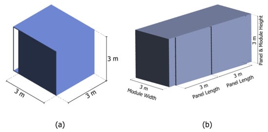
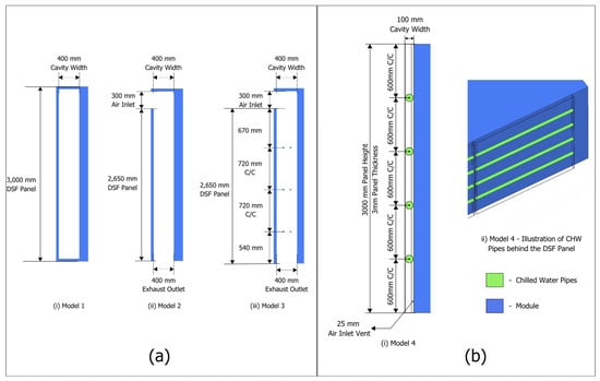
The first three double-skin façade (DSF) models were developed using a common reference façade geometry with dimensions of 3 m × 3 m × 3 m (length × width × height). A constant cavity width of 0.4 m was maintained between the primary façade and the DSF layer to ensure geometric consistency across these configurations. The baseline façade dimensions and cavity width were not chosen arbitrarily but adopted from representative values reported for double-skin façades assessed under hot-arid conditions. In particular, the 3 m module scale and the order of the cavity width follow the geometric range used by Sotelo-Salas et al. [32], who evaluated an opaque double-skin façade for cooling-load reduction in a hot-arid climate. Adopting dimensions consistent with an established hot-arid DSF study places the present models within a physically realistic geometric envelope for this climate context and ensures that the four configurations are compared at a façade scale representative of practical applications. The 0.4 m cavity retained across M1–M3 provides a fixed geometric baseline, so that the differences observed between these cases arise from the progressive addition of ventilation openings and cooling pipes rather than from a change in overall dimensions. The common computational domain is shown in Figure 2; retaining the same 3 m facade panel and 0.4 m cavity for M1–M3 ensures that differences among these cases arise from the addition of openings and CHW pipes rather than from a change in baseline scale.
Figure 2.
(a) Computational domain geometry for Models 1–3, showing the 3 m × 3 m × 3 m reference façade with 0.4 m cavity width between the primary façade and the DSF layer. (b) Isometric view of the Model 4 (M4) hybrid lateral DSF geometry, showing the dual aluminium panels.
The fourth DSF model was constructed with a separate geometric core to accommodate its larger façade system, as detailed in Section 2.3.4. The analysis focuses on the 3 m façade panel and the immediately adjacent cavity region rather than the full external enclosure of Model 4. This restriction reduces, but does not remove, the comparability limitations created by the different geometry, flow direction, cooling-surface area, and external domain.
A three-dimensional fluid enclosure was created in ANSYS DesignModeler to represent the surrounding air. The enclosure extended beyond each DSF geometry. The external air enclosure extended 2 m beyond the model surfaces in the two façade-plane directions and 0.2 m beyond the model in the vertical-clearance direction, giving an overall computational domain of approximately 7 m × 7 m × 3.4 m for Models 1–3 and approximately 11.19 m × 7 m × 3.4 m for Model 4. The outer boundaries were assigned a velocity inlet on the windward face, a pressure outlet on the leeward face, and symmetry or adiabatic no-slip wall conditions on the remaining faces, with the gauge pressure referenced to zero at the pressure-outlet boundary. The projected blockage ratio of the internal cooling-pipe surfaces relative to the cavity flow cross-section was 0.25% for the six 25 mm pipes of Model 3 and approximately 6.4% for the four 80 mm pipes of the narrow Model 4 cavity. The latter is of the same order as the 5% blockage guideline commonly adopted in related wind-driven CFD studies [33]; the slightly higher value reflects the deliberately confined lateral-flow geometry of the concept-stage Model 4, in which the lateral flow area available to the air exceeds the gap cross-section used in this conservative estimate.
2.3. DSF Model Geometries
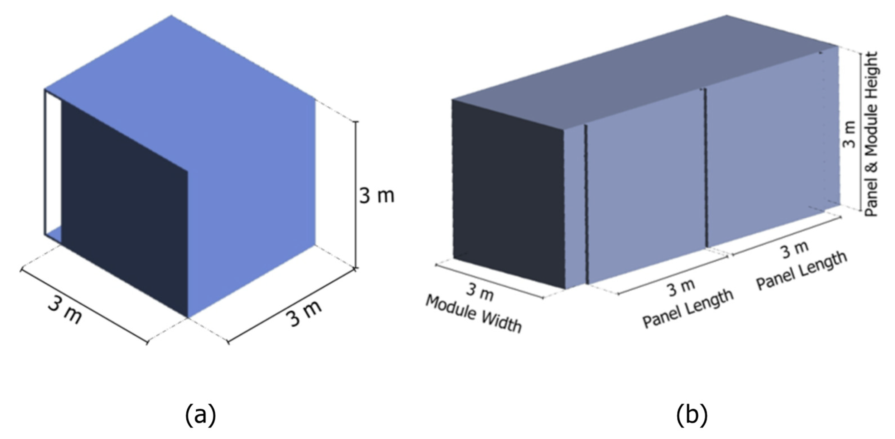
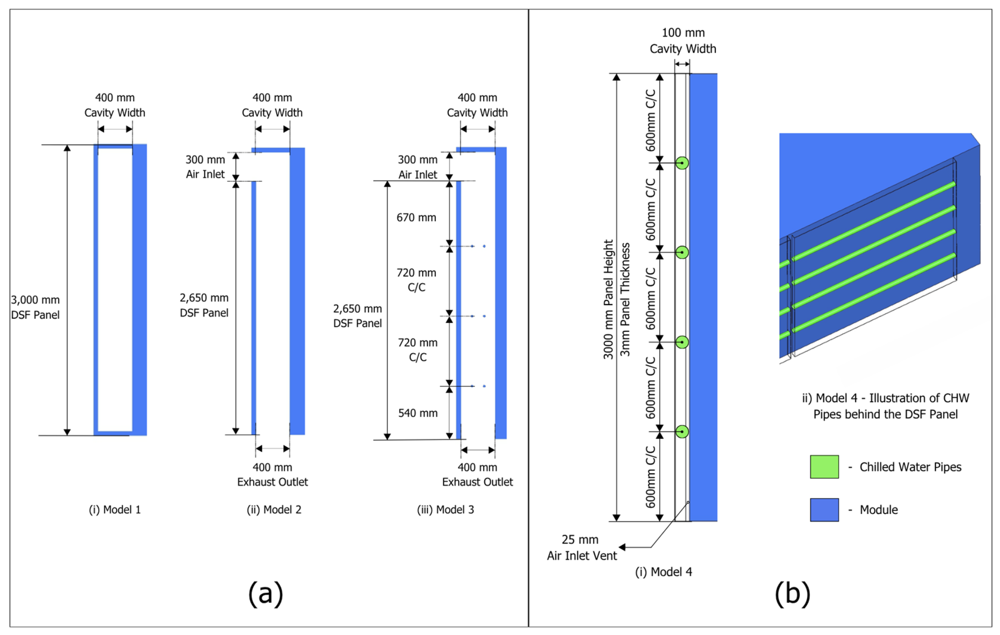
The controlled geometry sequence for the first three cases is shown in Figure 3. The figure clarifies that M1, M2 and M3 retain the same 0.4 m cavity envelope while progressively adding, first, top and bottom ventilation openings and, second, CHW pipe rows.
Figure 3.
(a) Sectional views of the first three DSF model geometries (M1–M3), illustrating the progressive introduction of ventilation openings and CHW pipes. (b) (i) Sectional view of the Model 4 (M4) geometry, showing the 0.10 m cavity depth, 0.025 m slit inlet, and pipe arrangement. (ii) Isometric view of the pipe arrangements behind the 3 mm thick DSF panel.
2.3.1. Model 1 (M1): Baseline Sealed DSF
Model 1 represents a conventional sealed double-skin façade with no ventilation openings or active cooling elements. The DSF’s outer skin has dimensions of 3 m (length) × 0.05 m (thickness) × 3 m (height). The cavity is fully enclosed, preventing airflow exchange with the external environment. This model serves as the baseline reference configuration.
2.3.2. Model 2 (M2): Ventilated DSF
Model 2 retains the same geometry as Model 1 but introduces rectangular ventilation openings to enable airflow exchange through the cavity. A top inlet and a bottom exhaust opening were incorporated into the DSF structure; the inlet had a width of 0.3 m, while the bottom exhaust opening measured approximately 0.4 m wide, with both openings extending across the 3 m panel length. This arrangement enables wind-driven airflow through the cavity without active cooling.
2.3.3. Model 3 (M3): Ventilated DSF with Chilled-Water (CHW) Pipes
Model 3 builds on Model 2 by integrating six chilled-water (CHW) pipe surfaces within the cavity. The pipes are arranged in two horizontal columns, with three pipes per column. Each pipe has a diameter of 0.025 m and a length of 3 m. The vertical spacing between adjacent pipes is 0.71 m centre-to-centre, while the horizontal spacing is 0.12 m centre-to-centre. The arrangement is shown in Figure 3. The actual airflow contact, pipe heat-transfer rate and water-side performance were not calculated; the pipes were represented only by a fixed surface-temperature boundary.
2.3.4. Model 4 (M4): Lateral-Flow Concept with Isothermal Cooling-Pipe Surfaces
The overall Model 4 concept geometry is introduced in Figure 2b, which shows the dual aluminium-panel arrangement. Unlike Model 3, Model 4 is not simply a ventilated cavity with additional cooling pipes; it is a distinct lateral-flow concept combining a narrower cavity, a different ventilation arrangement and larger isothermal cooling surfaces.
Model 4 is treated as a multivariable concept study rather than as a direct one-to-one comparator with Models 1–3 because it changes several parameters simultaneously, including cavity width, flow direction, panel arrangement, slit geometry, pipe diameter, pipe count and cooling-surface arrangement. Models 1–3 nevertheless provide useful reference cases representing sealed, wind-driven ventilated and ventilated-with-cooling configurations, respectively. These cases allow the predicted fields in Model 4 to be interpreted relative to simpler configurations, but they do not isolate the contribution of any individual Model 4 design variable. The purpose of Model 4 is therefore to examine the predicted temperature, velocity and turbulent kinetic energy fields of the combined concept, rather than to establish the independent effect of a particular geometric feature or to assess fabrication, installation or maintenance performance.
The Model 4 façade system includes two 3 m × 3 m aluminium panels, each 3 mm thick, installed parallel to one another with a panel-to-panel separation of 0.075 m. The detailed cavity section, slit inlet and cooling-pipe layout are shown in Figure 3b. The cavity between the outer aluminium skin and the building wall is 0.10 m wide, and ventilation is introduced through a 0.025 m-high lateral slit opening. This arrangement is intended to produce predominantly lateral airflow through the cavity. A detailed view of the slit-inlet geometry and pipe placement is provided in Appendix A, Figure A1.
Four isothermal cooling-pipe surfaces are installed within the cavity. Each pipe has a diameter of 80 mm and is oriented horizontally along the façade length. The pipes are distributed at equal centre-to-centre spacing along the façade height. Their water-side flow, water-temperature rise and cooling capacity were not modelled; instead, each pipe was represented by a fixed surface-temperature boundary.
The confined cavity and slit arrangement may influence airflow distribution and reduce some flow bypass, but this remains a design hypothesis because pathlines, residence time, cavity mass-flow distribution and pipe heat-transfer rates were not quantified.
2.4. Mesh Generation and Sensitivity Assessment
Mesh generation used predominantly unstructured tetrahedral elements to accommodate the ventilation openings and pipe surfaces. Prism (inflation) layers were applied near wall and pipe boundaries to improve near-wall resolution. The number, thickness, and growth of the prism layers, together with y+ values, were not reported; near-wall heat-transfer accuracy therefore cannot be confirmed from the mesh description alone.
A uniform global element size of 0.1 m was applied across all configurations. Local mesh refinement was introduced in regions of high velocity and thermal gradients, specifically near ventilation openings and pipe surfaces. Mesh quality was assessed using the skewness criterion, with a target maximum skewness value of 0.9.
The resulting mesh statistics are summarised in Table 1, which highlights the mesh-density increase associated with pipe surfaces and narrow-cavity refinement.
Table 1.
Mesh statistics for all four DSF configurations.
The larger mesh counts in Models 3 and 4 reflect the added pipe surfaces and local refinement. Face-sizing controls of approximately 2 mm were applied to the 3 mm aluminium panel surfaces and the 25 mm slit region in Model 4; approximate surface sizes of 5 mm and 10 mm were used on the M3 and M4 pipe surfaces, respectively; and the M2 vent regions were refined to approximately 10 mm. These controls provide additional local resolution but do not by themselves establish boundary-layer or solution independence. The global element size outside the refined regions was 0.1 m. Supplementary mesh views are provided in Appendix A Figure A2, Figure A3 and Figure A4.
A multi-level h-refinement check, similar in form to the approach cited in [34], was carried out. The global size was reduced from 0.15 m to 0.12 m and 0.09 m, and the area-averaged exit velocity changed from 3.54 to 3.51 and 3.49 m/s. The pairwise relative changes were 0.85% and 0.57%. These values indicate limited sensitivity of this single M2 velocity metric over the tested sequence; they are not a formal Grid Convergence Index and do not establish mesh independence for temperature, near-pipe heat transfer, Model 3 or Model 4. The grid-independence assessment was extended to five successively refined meshes, with the global element size reduced from 0.15 m to 0.06 m (Table 2). Following the h-method of [34], refinement was concentrated in the regions of steepest velocity and thermal gradient, and the area-weighted exit velocity was monitored between successive meshes; the pairwise relative change decreased monotonically from 0.85% to below 0.1% and fell below 0.5% at a global element size of 0.075 m, at which point the solution was taken to be grid-independent. Table 1 lists the production meshes used for each model’s final run, whereas Table 2 documents this dedicated refinement sequence for Model 2, generated across a range of global element sizes specifically for the independence study.
Table 2.
Mesh sensitivity check: area-averaged exit velocity and pairwise change across five meshes.
2.5. Solver Settings and Turbulence Modelling
All simulations were conducted using ANSYS Fluent 2025, employing a three-dimensional, pressure-based, steady-state solver. Gravity was enabled with a vertical acceleration of 9.81 m/s2 acting in the negative Z-direction. Air was modelled with constant properties: density 1.225 kg/m3, specific heat capacity 1006.43 J/kg·K and thermal conductivity 0.0242 W/m·K. Solid domains representing the façade panels were assigned aluminium properties of density 2719 kg/m3, specific heat capacity 871 J/kg·K, and thermal conductivity 202.4 W/m·K. The energy equation was activated. Because air density was fixed, temperature-driven buoyancy was not represented; enabling gravity alone does not introduce natural-convection density effects in this formulation. To assess whether neglecting buoyancy is acceptable, the Richardson number, Ri = gβΔTL/U2, was evaluated for the ventilated configurations, where β ≈ 1/T_film is the thermal expansion coefficient of air, ΔT = 26 K the imposed wall-to-wall temperature difference, L the cavity width and U = 3.06 m/s the reference inlet velocity. Using the cavity gap as the length scale, Ri ≈ 0.035 for the 0.4 m cavity (M2 and M3) and ≈ 0.009 for the 0.10 m cavity (M4); even with the full 3 m cavity height as the length scale, Ri ≈ 0.26. Since Ri < 1 in every case, forced (wind-driven) convection dominates over buoyancy, consistent with the natural, forced and mixed ventilation-mode classification established for double-skin façade cavities [9,17]; the constant-density assumption is a reasonable simplification for the ventilated cases, and the ideal-gas density variation was addressed theoretically through this criterion rather than through an additional variable-density simulation. This argument does not extend to the sealed baseline (M1), in which the absence of forced flow means buoyancy would be the dominant transport mechanism; the M1 field is therefore presented only as a conductive, fixed-boundary reference, and a buoyancy-resolved (Boussinesq or ideal-gas) simulation of the sealed cavity is identified as future work.
Turbulence was modelled using the standard k-ε model with standard wall functions as a baseline Reynolds-averaged closure. The narrow-channel study cited in [35] concerns a different, calibrated rib-roughened configuration and should not be treated as validation of the present DSF models. No turbulence-model sensitivity or y+ assessment was performed, so predictions in the narrow cavity and near cooled surfaces remain subject to model-form and wall-treatment uncertainty. Pressure–velocity coupling used a segregated pressure-correction scheme, with second-order upwind discretisation for momentum, energy and turbulence. Simulations were run for 2000 iterations and were reported as converged when momentum and continuity residuals were below 1 × 10⁻⁴ and the energy residual was below 1 × 10⁻⁶.
2.6. Boundary Conditions
A common set of idealised, steady-state boundary conditions was applied to all four models. These conditions represent a single extreme hot-arid design point rather than a typical or time-varying Dubai climate condition. A uniform external airflow of 3.06 m/s at 323.15 K (50 °C) was imposed at the windward velocity-inlet boundary, while the leeward boundary was defined as a pressure outlet at 0 Pa gauge pressure. The imposed external flow generated wind-driven exchange through Models 2 and 3 and wind-driven slit inflow in Model 4; Model 1 remained sealed.
The exterior DSF surface was assigned a fixed temperature of 323.15 K (50 °C) and a no-slip condition. This temperature was selected as a prescribed severe thermal boundary representing a sun-heated exterior surface under an extreme hot-arid condition, consistent with the high solar gains and elevated façade-surface temperatures reported for such climates [1,10,11]. It was not calculated from a coupled solar-radiation or exterior-surface energy balance and should therefore not be interpreted as a predicted façade-surface temperature. Applying the same exterior air and surface temperatures to all four configurations provided a common thermal forcing for the comparative analysis. However, the model does not capture variations in solar angle, time of day, surface optical properties, long-wave radiative exchange or diurnal environmental conditions. The reported fields should consequently be interpreted as responses to a fixed design point rather than as predictions of in situ façade performance. Coupled solar-radiation modelling and transient boundary conditions are recommended for future work.
The interior-side wall was assigned a fixed temperature of 297.15 K (24 °C) and a no-slip condition. This boundary represents a prescribed interior surface temperature rather than a coupled simulation of room air, occupant comfort or HVAC-system response. Air was modelled with constant density; therefore, temperature-driven buoyancy and natural ventilation were not represented. The ventilated configurations should accordingly be interpreted as wind-driven cases.
Inlet turbulence was specified using a turbulent kinetic energy of 0.0351 m2/s2 and a dissipation rate of 0.759 m2/s3. The cooling-pipe surfaces in Models 3 and 4 were assigned a constant temperature of 283.15 K (10 °C). They therefore represent idealised isothermal cooling surfaces rather than a coupled chilled-water circuit; water flow rate, pipe-wall heat transfer, water-temperature rise, cooling capacity and pumping energy were not modelled.
The remaining domain boundaries were assigned symmetry or adiabatic no-slip wall conditions, as applicable. For the open-domain configurations, the inlet-to-outlet mass-flow imbalance remained below 1%. An energy-imbalance value was not reported. Although the prescribed external velocity and wall temperatures were common to the models, the configurations differed in geometry, opening arrangement, flow direction, pipe diameter and cooled-surface area. Differences in the predicted fields therefore reflect the combined effects of these changes within the adopted modelling assumptions and should not be attributed to a single isolated variable. Table 3 summarises the prescribed boundary values.
Table 3.
Summary of boundary conditions applied to all DSF configurations.
2.7. Data Extraction and Analysis
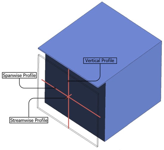
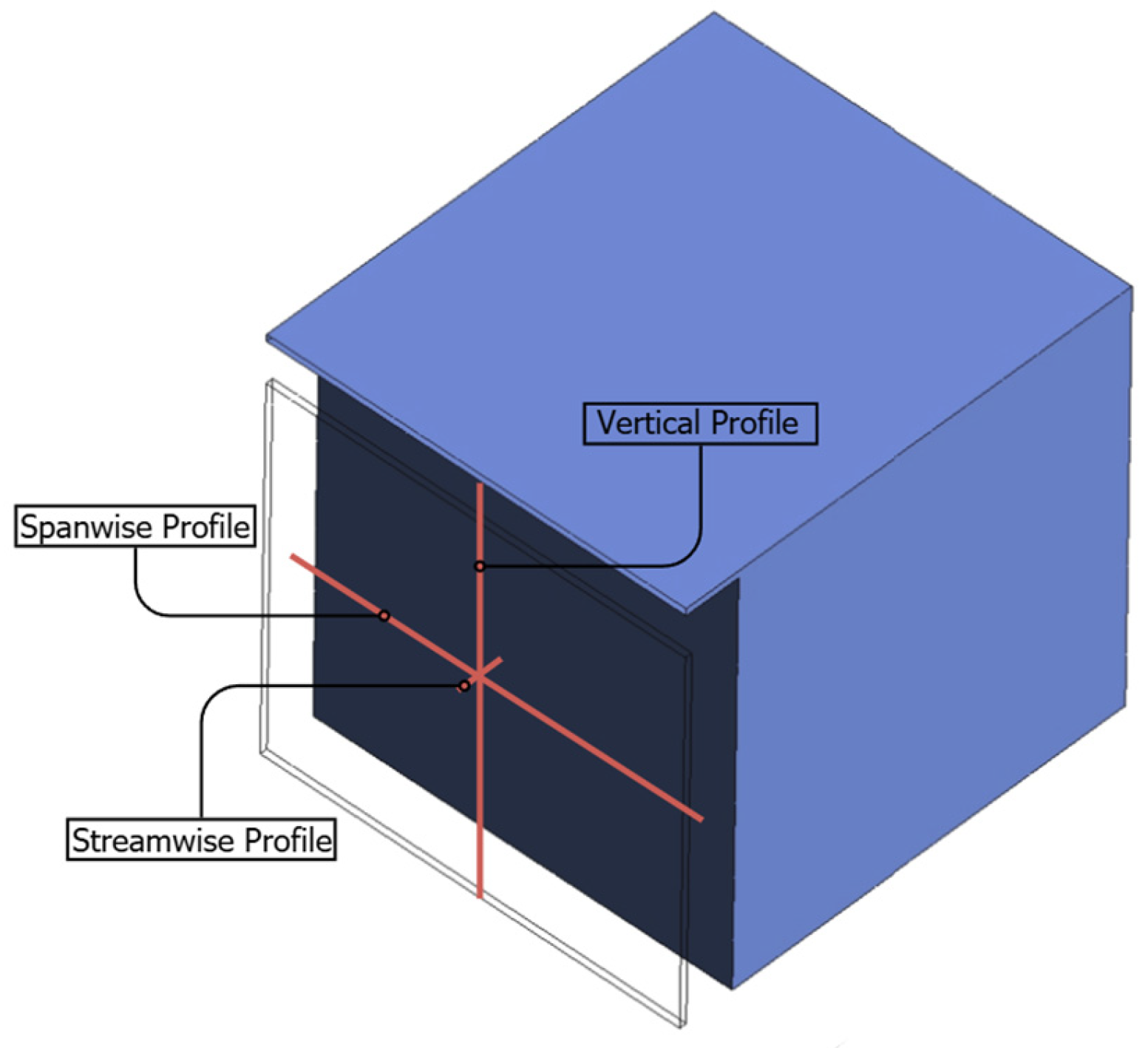
After the stated residual criteria were met, the simulations were post-processed to extract air temperature, velocity magnitude and turbulent kinetic energy (TKE) on selected lines and planes. These outputs describe local and sectional field patterns. They are not cavity-volume averages, mass-weighted outlet values, heat-transfer rates or energy balances. Analogous, rather than geometrically identical, sampling locations were used across the different configurations; the probe directions are defined in Figure 4.
Figure 4.
Schematic of line-probe orientations: streamwise across cavity depth, spanwise horizontally along the façade at the selected plane, and vertical from top to bottom.
A line was defined across the cavity depth between the outer and inner surfaces at a selected height. This across-cavity line is termed the streamwise direction (sampled from the outer skin toward the inner wall at the selected plane). Temperature, velocity and TKE along this line describe spatial variation across the gap; they are not cavity averages. A horizontal line was placed at the selected mid-height plane along the façade direction. This horizontal façade-direction line is termed the spanwise direction. In Model 4, this line approximately aligns with the intended lateral flow path. In Models 1–3, it is a horizontal façade-direction sample and should not be described as the vertical primary-flow path. A line through the cavity extended from the top to the bottom. This top-to-bottom line is termed the vertical direction. It describes vertical variation and may intersect vent- or pipe-influenced regions. Because the air density was held constant, the profile does not demonstrate buoyancy-driven stratification. A horizontal plane at the selected height was used to plot temperature, velocity and TKE. Fields plotted on this horizontal plane are termed the aerial or plan-view field. These contours show two-dimensional spatial patterns at that plane only. Line data were exported to CSV files and graphed in Microsoft Excel. Probe-point indices are normalised and do not represent the same physical spacing or direction in every model. Contour scales differ among several figures and are stated in the captions; visual colour comparisons across different scales should therefore be made cautiously. Where per-model colour scales are used, in particular for the temperature and TKE contours, these ranges were pre-determined deliberately so that the local low-temperature and localised turbulence detail near the 10 °C cooling-pipe surfaces in Models 3 and 4 remains visible; a single common scale spanning the full 10–50 °C range would compress and obscure these local features. Each figure states its scale in the caption, and quantitative comparisons between models are based on the extracted line-profile values rather than on colour magnitude.
3. Results
This section presents predicted fields for four DSF configurations under an idealised steady-state design point with 50 °C external air and outer-wall temperatures and a 3.06 m/s external inlet. Model 1 is sealed; Model 2 is wind-driven and ventilated; Model 3 adds six 25 mm isothermal cooling pipes; and Model 4 is a multivariable lateral-flow concept with a 0.10 m cavity, a 0.025 m slit, and four 80 mm isothermal cooling pipes. The case does not represent the complete Dubai climate or a building-energy calculation.
Temperature, velocity and modelled TKE are reported from selected line profiles and contour planes. These fields help describe where the model predicts warmer, cooler, faster or more turbulent regions, but they do not quantify heat removed before it reaches the building interior. The streamwise line crosses the cavity depth, the vertical line runs top-to-bottom, and the spanwise line is horizontal; only in Model 4 does the spanwise line approximately follow the intended primary lateral flow.
Each line profile contains 100 normalised sample points, but the physical line lengths and orientations differ among models. Point number therefore does not correspond to an equal physical distance across cases. The profiles are used descriptively, and no line should be interpreted as a cavity-volume average.
3.1. Temperature Field and Comparative Description
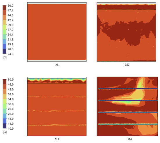
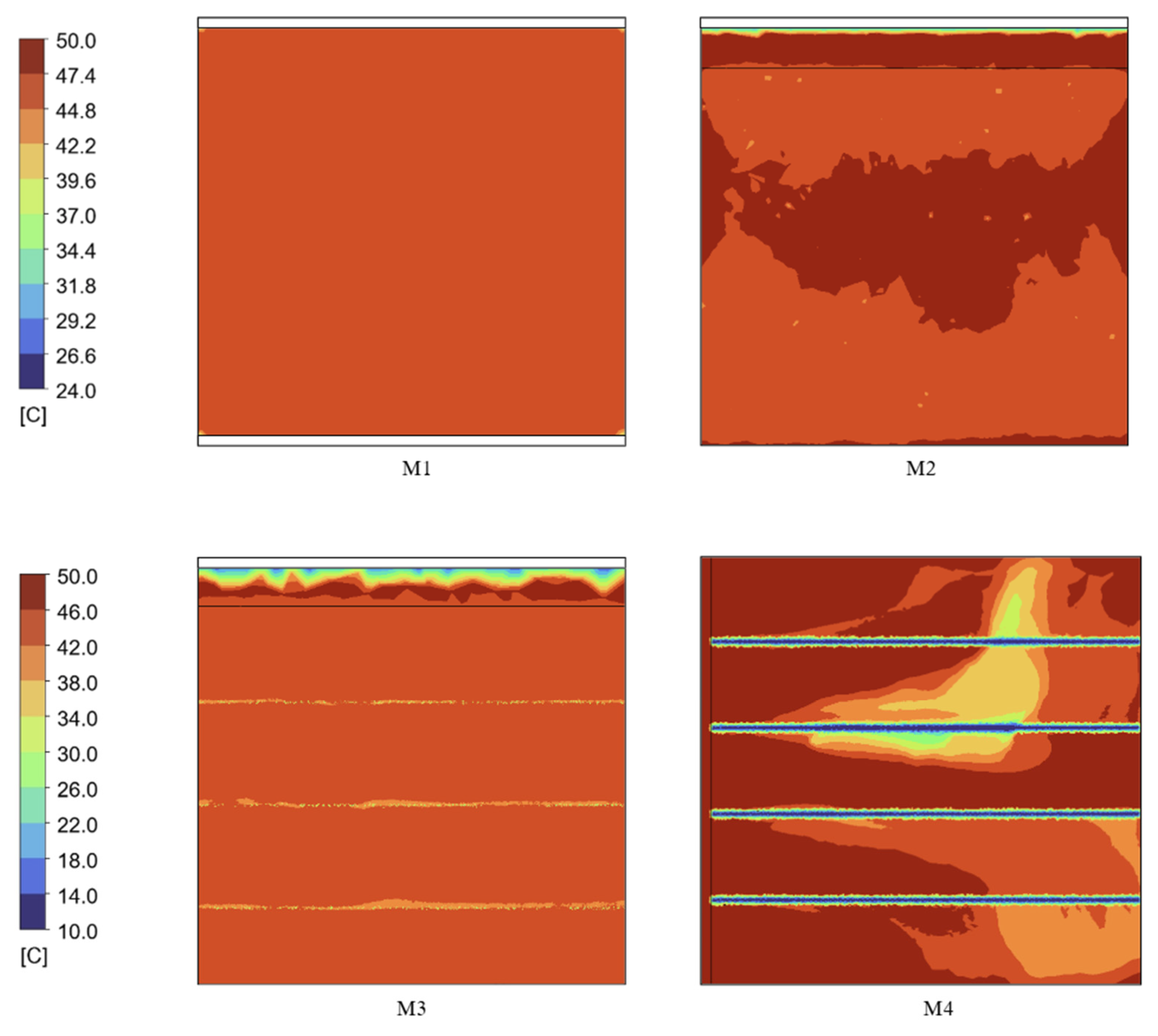
Figure 5 and Figure 6 show selected temperature contours and spanwise line profiles. Because the contour scales differ and the spanwise probe has different alignment relative to the primary flow in Models 1–3 and Model 4, the figures support a qualitative comparison of field patterns rather than an overall performance ranking.
Figure 5.
Spanwise temperature contours for Models 1–4 at the selected cross-section. Models 1 and 2 use a 24–50 °C scale, while Models 3 and 4 use a 10–50 °C scale to show local low-temperature regions near the 10 °C isothermal pipe surfaces. Colour magnitudes should not be compared directly across the two scales.
Figure 6.
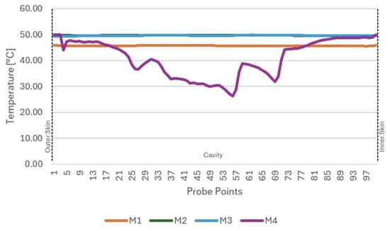
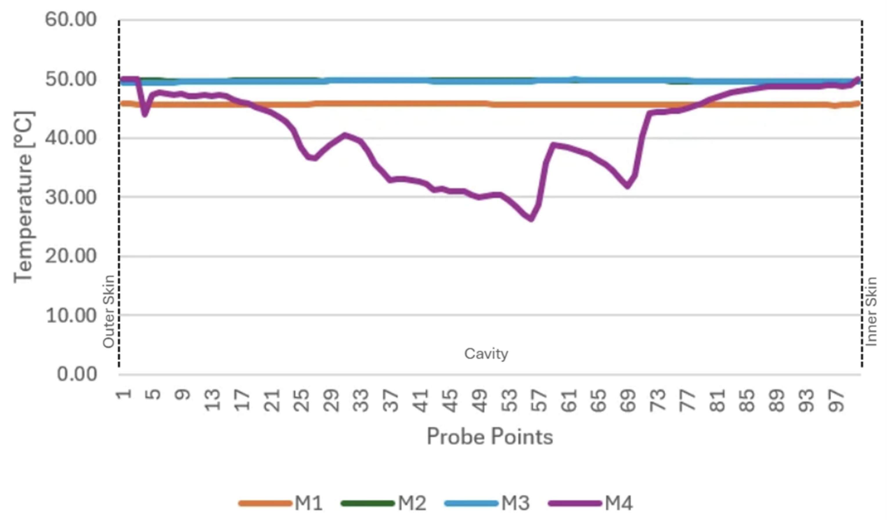
Temperature profiles on the reported spanwise lines for Models 1–4 at the selected cavity plane. The line approximately follows lateral flow in Model 4 but is not the vertical flow path in Models 1–3. Each profile contains 100 normalised sampling points.
Figure 5 and Figure 6 show clear differences in the sampled temperature fields, but they do not establish a hierarchy of whole-cavity thermal performance. The reported ranges are line-based spatial samples and include local boundary- and pipe-influenced values. Supporting temperature plots are provided in Appendix A Figure A5, Figure A6, Figure A7 and Figure A8.
Model 1 shows a nearly uniform predicted temperature on the selected profiles: 45.73–45.74 °C streamwise, 45.51–45.92 °C spanwise, and 45.70–45.99 °C vertically. This is the steady-state result of the imposed 50 °C outer boundary and 24 °C inner boundary in a sealed cavity. The approximately 4.1–4.5 °C difference below the 50 °C boundary should not be interpreted as passive cooling capacity, energy savings or an upper bound for DSF performance, because no heat flux, radiation, or building load was calculated.
Model 2 shows temperatures close to the prescribed 50 °C external condition on the selected lines. The reported spanwise range is 49.57–49.73 °C, the streamwise range is 46.46–49.76 °C, and the vertical range is 48.53–49.70 °C. These values describe local positions in a wind-driven ventilated cavity. They do not demonstrate heat-accumulation prevention, residence time or poorer overall performance than the sealed case, because neither a volume average nor a heat balance was reported.
In Model 3, the reported spanwise line remains near 50 °C at 49.38–49.86 °C, while the summary table reports a wider streamwise range of 43.80–49.09 °C and a vertical range of approximately 46–49.09 °C. The lower values occur where the selected probes and planes intersect pipe-influenced regions. These profiles indicate spatially local cooling effects but do not provide a whole-cavity average or cooling rate.
The Model 3 contours contain lower-temperature bands near the isothermal pipe surfaces and warmer regions between them. This pattern is consistent with a local influence from the cooling surfaces. It does not by itself quantify airflow bypass, residence time, or how much of the total airflow is cooled. Locally sampled air temperatures in the mid-20s Celsius are reported near the pipes, while the pipe surfaces were fixed at 10 °C.
Model 4 shows the widest temperature spread on the selected profiles: 26.90–50 °C on the spanwise line and 28.6–49.36 °C across the cavity depth, with local pipe-adjacent air values reported near 24 °C. Here, pipe-adjacent (also termed pipe-proximal) denotes an air value sampled near a cooling-pipe surface; it is not the pipe-surface temperature, which was fixed at 10 °C, or a cooling-capacity measure. These are local spatial ranges and minima, not a bulk cavity temperature or a 23 °C whole-cavity reduction. The vertical profile contains sharp local minima where it intersects pipe-influenced regions; it does not support a claim that most of the vertical extent is sustained at 12–35 °C.
The Model 4 contours show broader lower-temperature regions on some selected planes and a lateral variation from warmer to cooler zones. This is consistent with the combined influence of the narrower cavity, larger cooling surfaces, different pipe arrangement and lateral inlet. The simulations do not isolate which change is responsible, nor do they demonstrate that every air parcel contacts the cooled surfaces or that bypass is eliminated. Mass-flow distribution, pathlines, residence time and heat flux would be needed to support those mechanisms.
3.2. Velocity Field and Comparative Description
Figure 7 and Figure 8 present selected velocity contours and spanwise line profiles. The profiles describe local velocities on the reported lines; they are not mass-flow rates and, for Models 1–3, the spanwise line is not the full vertical inlet-to-outlet path.
Figure 7.
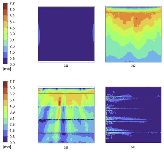
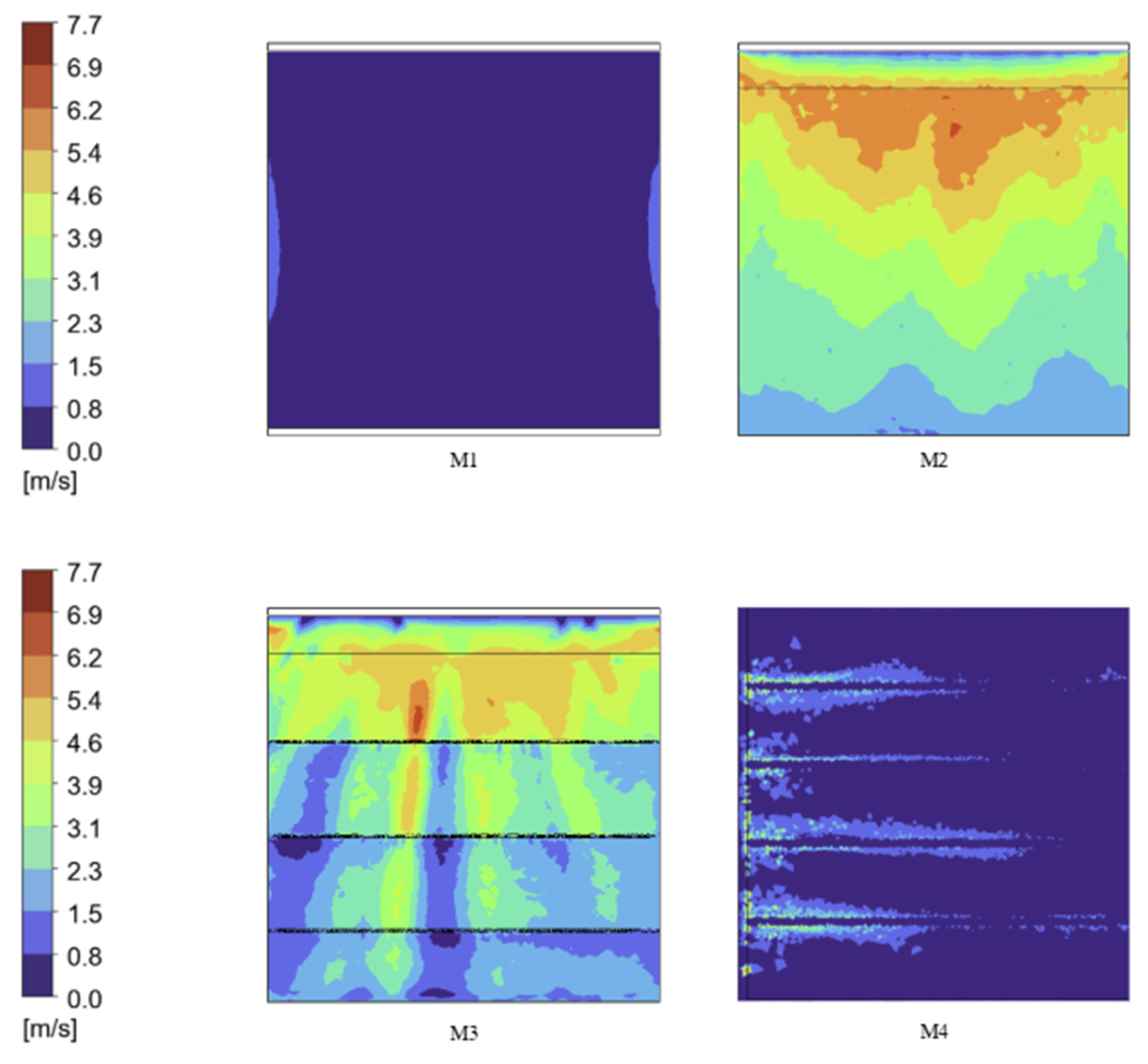
Spanwise velocity contours for Models 1–4 at mid-height cross-section. Note: All four models share a common contour scale of 0–7.7 m/s, set by the maximum velocity in the external flow domain. This unified scale permits direct visual comparison of cavity-interior velocities across configurations.
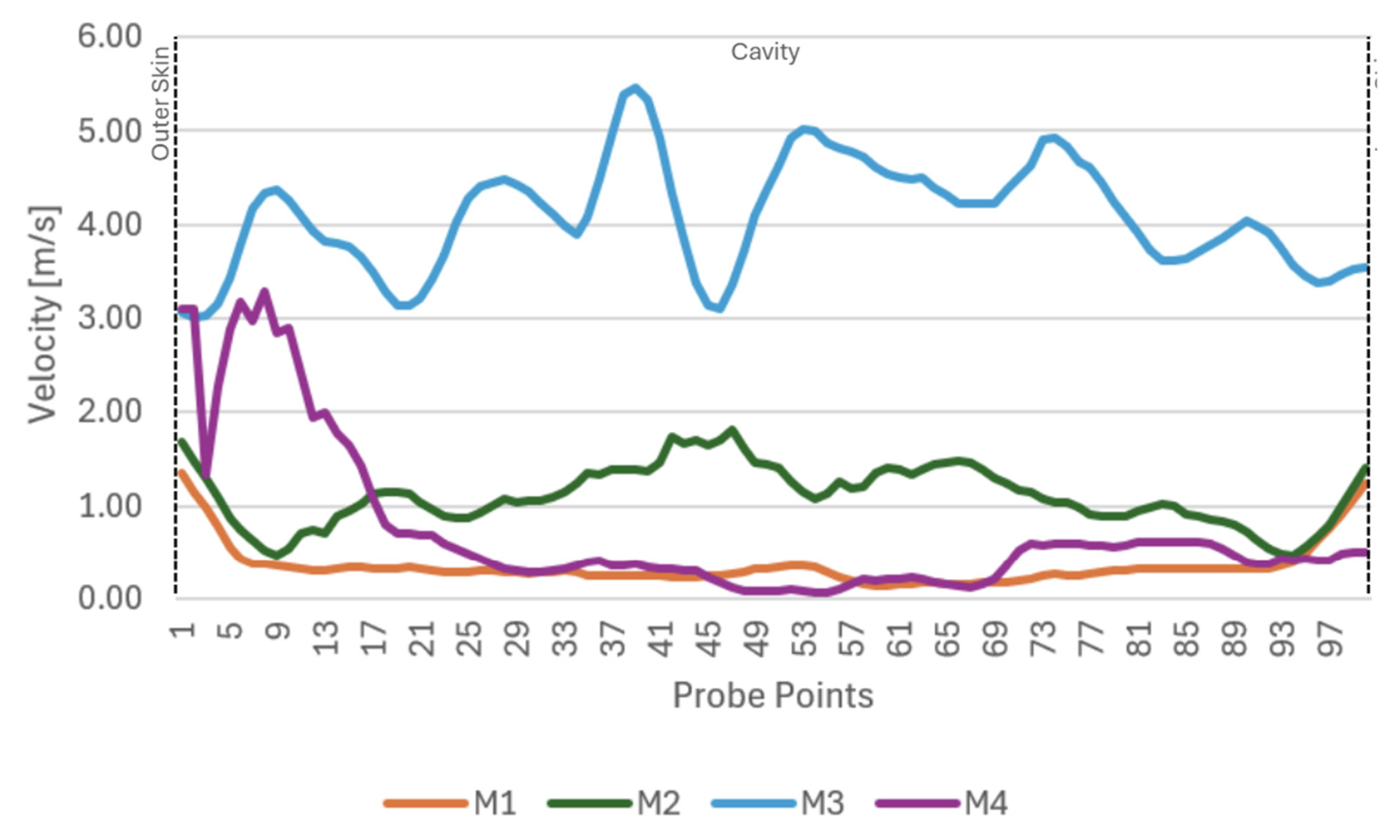
Figure 8.
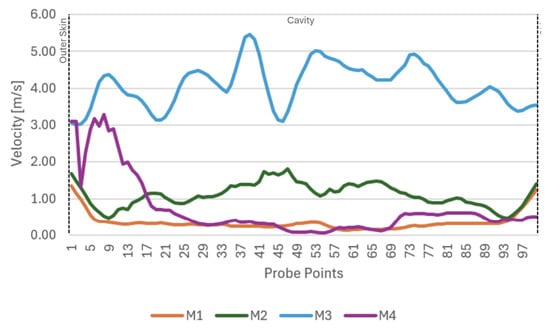
Velocity profiles on the reported spanwise lines for Models 1–4 at the selected cavity plane. The physical alignment relative to the primary flow differs among models. Each profile contains 100 normalised sampling points.
The computed velocity fields differ substantially among the configurations. Higher- or lower-sampled velocity can be compared descriptively with the temperature field, but correlation between two selected profiles does not establish the cause of the temperature pattern. Supporting velocity plots are provided in Appendix A Figure A11, Figure A12, Figure A13 and Figure A14.
Model 1 has low but non-zero computed velocities on the selected profiles: 0–0.48 m/s streamwise, 0.15–0.35 m/s spanwise and up to about 0.42 m/s on the aerial plane. Because the cavity is described as sealed and the constant-density model does not include thermal buoyancy, these residual velocities should be interpreted cautiously as numerical or local model behaviour rather than evidence of a physically validated recirculation mechanism. No conclusion about convective heat transfer can be drawn from these values alone.
Model 2 shows wind-driven motion through the ventilated cavity. The reported streamwise range is 0–5.75 m/s, the spanwise range is 0.81–1.81 m/s, and the vertical profile reaches 0.81–4.31 m/s. The vertical profile and contours, rather than the horizontal spanwise line, provide the relevant indication of top-to-bottom exchange. No cavity mass-flow rate or residence time was extracted, so the effect of turnover on heat transfer is not quantified.
Model 3 shows local acceleration and deceleration around the pipe obstructions. The reported streamwise range is 0–5.16 m/s, the spanwise range is 3.15–5.45 m/s, and the vertical range is 2.18–5.72 m/s. The higher values on the M3 spanwise line relative to M2 do not establish a greater total mass flow, because the line locations and flow distributions differ, and mass flow was not calculated.
The Model 3 contours show faster regions between or around pipe rows and lower-velocity regions in their wakes. These patterns are consistent with local obstruction effects. The present outputs do not demonstrate that high velocity causes airflow bypass or that local shear is responsible for the reported temperature minima; those interpretations would require pathlines, heat fluxes and mass-flow-resolved analysis.
In Model 4, the geometry produces a local slit-associated acceleration and lower velocities over parts of the lateral cavity. The reported spanwise range is 0–3.10 m/s, the streamwise range is 0–0.21 m/s, and the vertical profile reaches 0–1.80 m/s. The extrema depend on the selected plane and line and should not be treated as representative cavity velocities.
The Model 4 contours suggest an entry jet followed by lower-velocity regions farther into the cavity, with local acceleration near pipe gaps. This pattern may be relevant to heat exchange, but no residence time, pressure drop or mass-flow rate was reported. The velocity field therefore does not establish that the flow has sufficient dwell time or that post-entry deceleration causes the lower sampled temperatures.
Qualitative Pressure Field (M4)
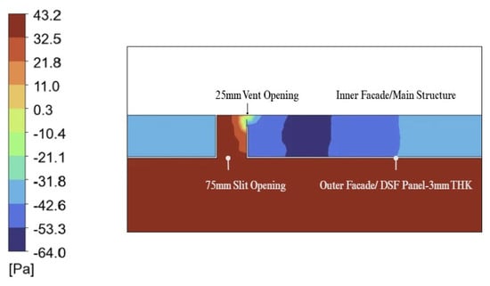
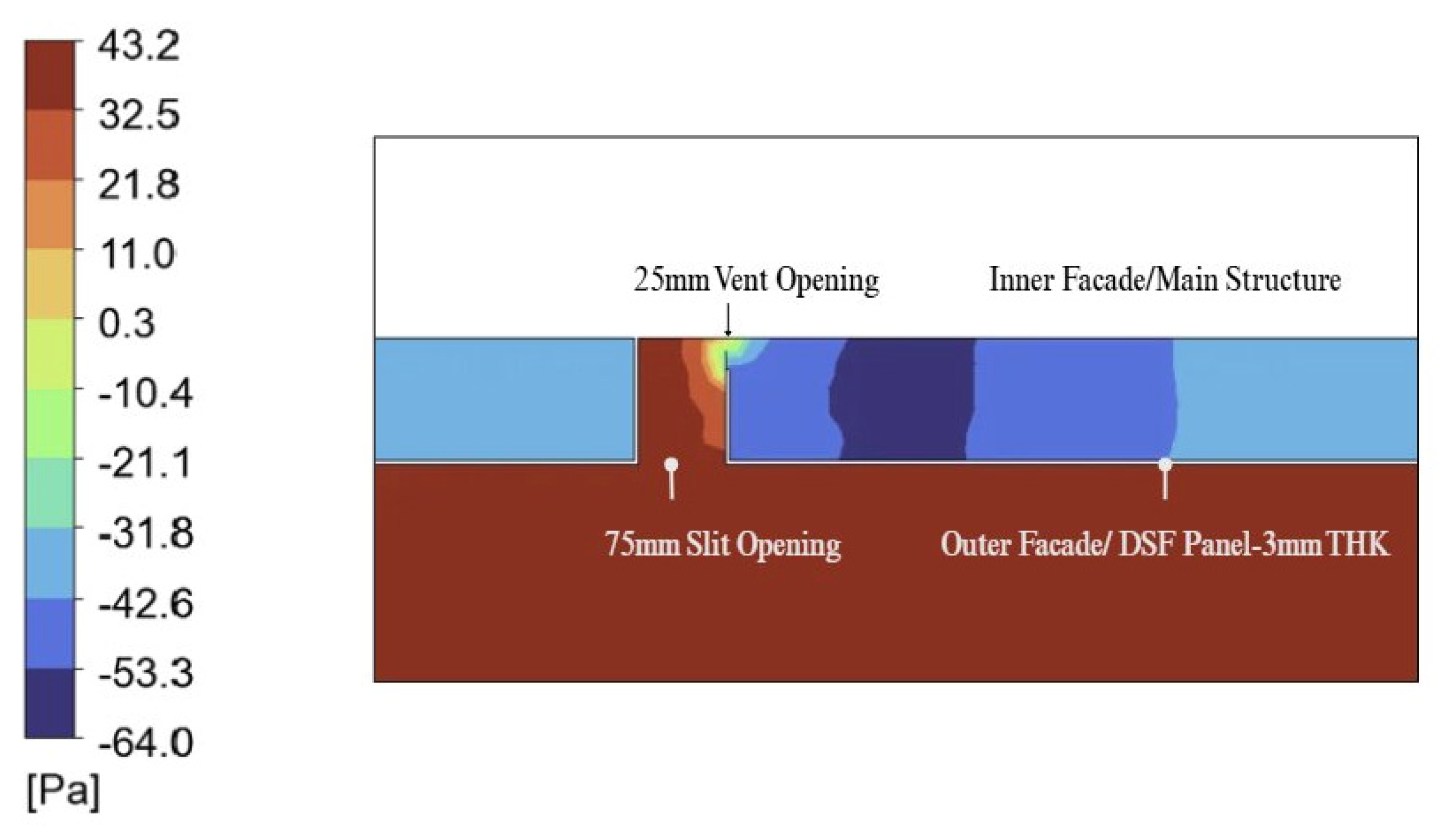
Figure 9 shows gauge-pressure variation near the Model 4 slit. The plotted scale ranges from approximately +43 to −64 Pa. Using the specified air density and 3.06 m/s inlet velocity, the nominal inlet dynamic pressure is about 5.7 Pa; the much larger plotted range therefore requires clarification of the pressure reference, boundary placement and solver setup before it can be interpreted as a physical pressure drop. The figure is used here only to indicate a qualitative pressure gradient near the opening.
Figure 9.
Gauge static-pressure contour near the Model 4 slit. The absolute plotted range is used qualitatively only; a validated pressure drop cannot be inferred without a documented pressure reference and mass-flow balance.
No mass-flow rate through the slit, pressure-drop monitor, or flow balance was extracted. The present results therefore support only the qualitative observation that the imposed external-flow boundary produces a pressure gradient and local acceleration near the slit. Future work should report mass flow, pressure drop, and sensitivity to the external-domain boundaries before characterising the flow driver quantitatively.
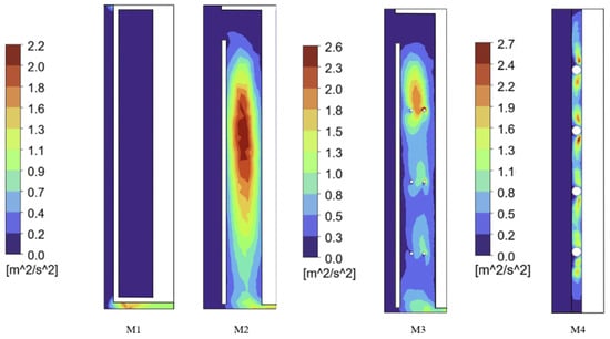
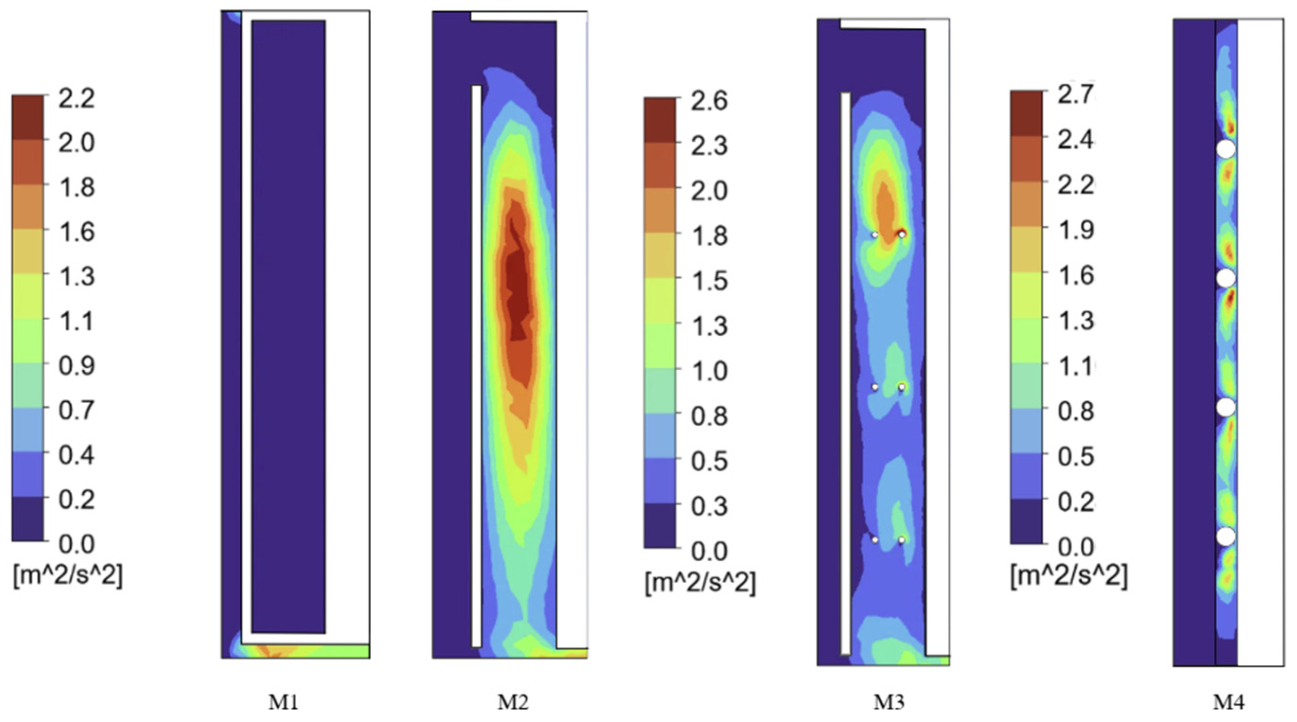
3.3. Turbulent Kinetic Energy Field and Comparative Description
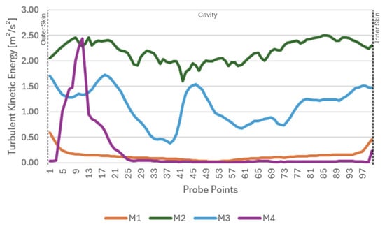
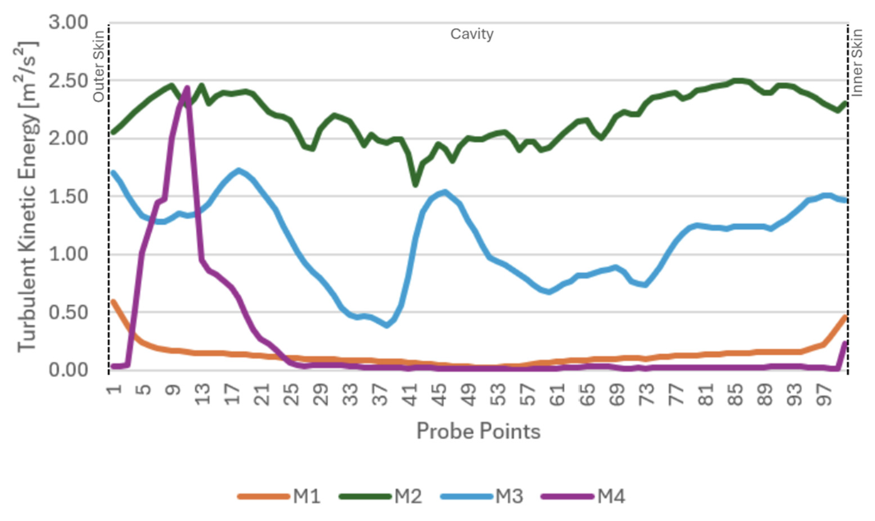
Figure 10 and Figure 11 present modelled TKE contours and spanwise line profiles. TKE is an output of the selected RANS turbulence model; it is used to describe the modelled distribution of turbulent fluctuations, not to classify the flow as laminar or to measure mixing experimentally.
Figure 10.
Spanwise TKE contours for Models 1–4 at the selected cross-section. Each model uses an independently auto-scaled range (M1/M2: 0–2.2 m2/s2; M3: 0–2.6 m2/s2; M4: 0–2.7 m2/s2). The contours may be compared for spatial pattern, but colour magnitudes should not be compared directly across models.
Figure 11.
TKE profiles on the reported spanwise lines for Models 1–4 at the selected cavity plane. The physical alignment relative to the primary flow differs among models. Each profile contains 100 normalised sampling points.
The selected profiles show that modelled TKE and sampled temperature are not positively correlated in a simple way across the four cases. Model 2 has higher reported TKE on several lines while its sampled temperatures remain near 50 °C, whereas Model 4 combines low TKE on some core lines (here, core lines denote the central portion of a line or plane away from obvious boundaries—local samples rather than volume averages) with local lower-temperature zones. Because the probe directions differ and Model 4 changes several variables at once, these observations do not establish that geometric confinement governs performance or that turbulence is unimportant. Supporting TKE plots are provided in Appendix A Figure A17, Figure A18, Figure A19 and Figure A20.
Model 1 records low modelled TKE on the selected profiles: 0.02–0.03 m2/s2 streamwise, 0.03–0.10 m2/s2 spanwise and 0–0.03 m2/s2 vertically. These values indicate low TKE in the RANS solution but do not, by themselves, establish a laminar flow regime. The non-zero values should also be interpreted in light of the sealed geometry and the absence of buoyancy modelling.
Model 2 has the highest reported TKE on several selected lines: 0.36–2.03 m2/s2 streamwise, 1.59–2.50 m2/s2 spanwise and 0.13–2.22 m2/s2 vertically. The contours show broad regions of elevated modelled TKE. At the same time, the selected temperature profiles remain close to the 50 °C boundary condition. This supports the limited observation that higher modelled TKE did not coincide with lower sampled temperature in this case; it does not show that turbulence merely redistributes heat or that it cannot contribute to heat transfer.
Model 3 shows TKE variations associated with the pipe rows. The reported ranges are 0.11–0.84 m2/s2 streamwise, 0.46–1.51 m2/s2 spanwise and 0.05–1.12 m2/s2 vertically. The contours contain local bands and peaks near some pipe-influenced regions.
The local TKE peaks in Model 3 are consistent with flow disturbance around the pipe obstructions. The available results do not quantify whether those peaks increase pipe heat transfer or explain the temperature pattern, because wall heat flux and coupled local correlations were not reported. The observation should therefore remain descriptive rather than being used as evidence for a general geometric-confinement mechanism.
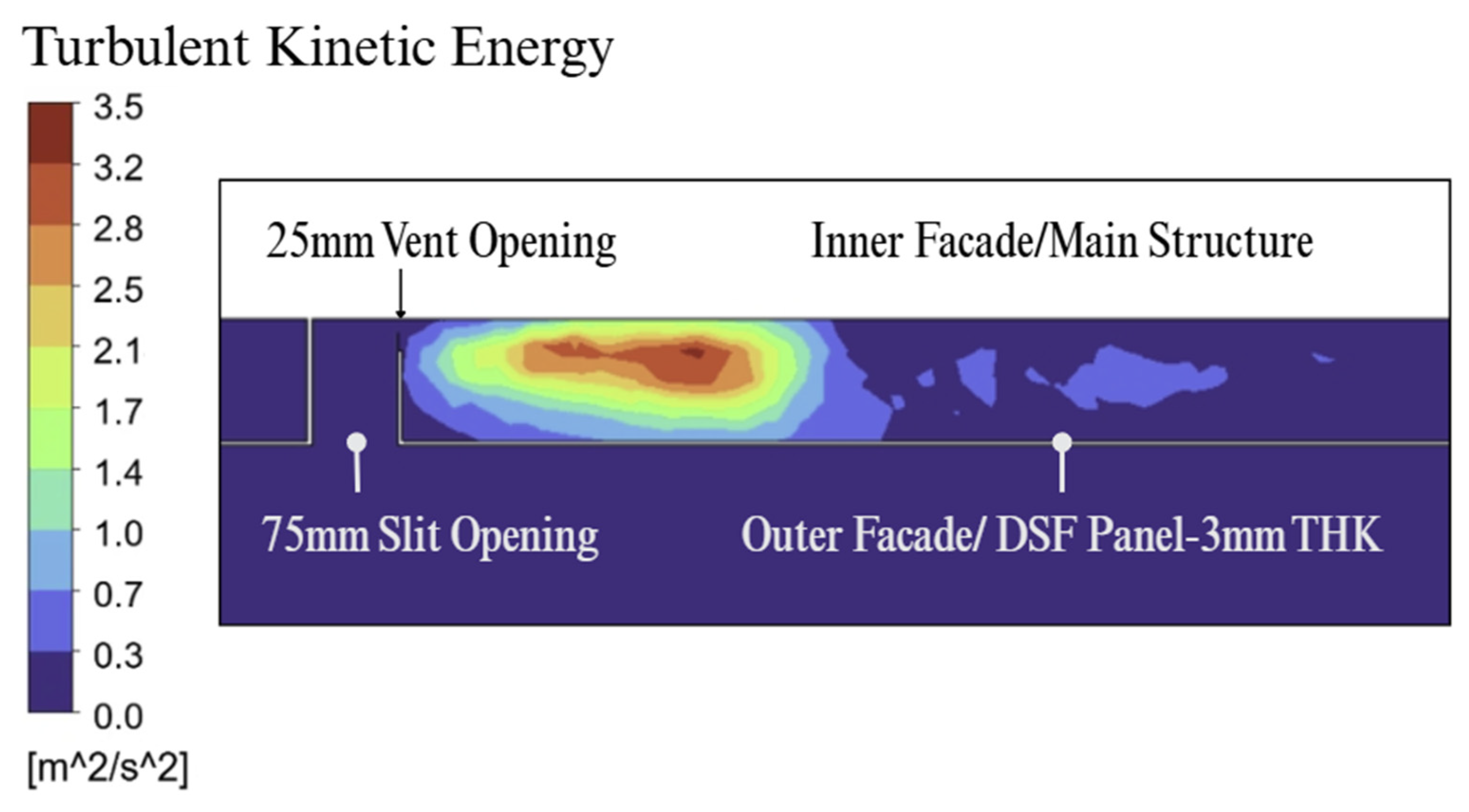
Model 4 has low modelled TKE on the selected streamwise and vertical core lines, with reported ranges of 0–0.01 m2/s2 and 0–0.17 m2/s2, while the spanwise line reaches 0.2–2.44 m2/s2 near entry- and pipe-influenced locations. The values indicate a spatially non-uniform TKE field rather than a uniformly calm or laminar cavity.
The Model 4 contours show local TKE peaks near the slit and pipe locations and lower values over other portions of the selected planes. These patterns do not demonstrate a deliberate boundary-layer-disruption mechanism, longer contact time or a causal link to the temperature minima. Establishing such links would require local wall heat fluxes, pathlines, residence-time or scalar-transport analysis and comparison with otherwise identical geometries.
3.4. Interpretation and Design Hypotheses
Models 1–3 share a 0.4 m cavity envelope but differ in openings and cooling surfaces. On the reported spanwise lines, M2 and M3 remain close to 50 °C, while M3 also shows local lower-temperature regions near pipes on other lines and contours. These observations describe the selected fields only. They do not provide a whole-cavity cooling metric and should not be used to rank the thermal performance of the configurations.
Model 4 produces broader lower-temperature regions on some selected planes and the lowest local line values in the study. It also differs from M3 in cavity width, flow direction, slit geometry, pipe diameter, pipe count, cooled-surface area, and panel arrangement. The results therefore support a hypothesis that the combined lateral-flow concept merits controlled study; they do not show that narrowing the cavity alone eliminates bypass or produces a 23 °C bulk reduction.
Across the selected profiles, TKE magnitude is not a sufficient predictor of sampled temperature. This observation motivates further examination of airflow distribution, cooled-surface exposure and integral heat transfer. However, air-surface contact time was not calculated, and the present comparison cannot establish that geometric strategies are more effective than turbulence-management strategies in general.
The fixed 10 °C pipe boundaries in Models 3 and 4 create local low-temperature regions, as expected for isothermal cooling surfaces. The M3-M4 comparison does not isolate cavity geometry because the cooling-surface dimensions and arrangement also change. It therefore cannot establish that active cooling is essential, that one configuration outperforms the other, or that cooling is distributed across the entire cavity volume.
3.5. Comparability of the Extracted Profiles
All reported line profiles contain 100 sample points. A shorter physical line therefore has smaller point spacing, not fewer points. The principal comparability issue is instead that the lines have different physical lengths and, in the case of the spanwise profiles, different alignment relative to the primary flow. Normalised probe indices should not be interpreted as common spatial coordinates across models.
The line ranges and contours are therefore used as descriptive local evidence. A stronger comparison would report the physical coordinates of each probe, cavity-volume averages, mass-weighted inlet and outlet temperatures, mass flow, wall and pipe heat fluxes, pressure drop, and conservation balances. Without those quantities, the analysis should avoid whole-cavity cooling claims and overall rankings.
3.6. Summary of Reported Metrics
Table 4 and Table 5 consolidate the reported line-profile ranges, local minima and geometric descriptors. They are descriptive summaries and do not represent volume-averaged performance, heat-removal rates or an overall cooling ranking.
Table 4.
Reported line-profile ranges and local temperature minima.
Table 5.
Geometry and qualitative field descriptors; no overall performance ranking is assigned.
Within the adopted assumptions, Model 4 shows the widest sampled temperature range and the lowest local temperatures on the reported probes. Because the concept changes multiple variables and no heat-removal or energy metric was calculated, this observation should not be described as superior cavity-level thermal management.
4. Discussion
This section discusses the temperature, velocity and turbulent kinetic energy fields reported in Section 3 in terms of their contribution and scope, their implications for further development, the limitations of the present study, and the resulting recommendations for future work. Table 6 provides a summary of the outputs and their interpretive limits.
Table 6.
Summary of reported local and line-profile outputs and their interpretive limits.
The four configurations serve distinct roles in the comparison. M1 functions as a sealed thermal reference that fixes the purely conductive cavity equilibrium under the common boundaries. M2 isolates the effect of wind-driven ventilation: on the reported lines, its temperatures remain close to the 50 °C external condition, indicating that, under the fixed-density formulation and the prescribed inlet, ventilation alone does not lower the sampled cavity temperature, although it raises the modelled turbulence field. M3 adds isothermal cooling pipes to the same ventilated cavity: it introduces local low-temperature regions in the immediate vicinity of the pipes while the wider spanwise line remains near ambient, so its thermal impact is spatially confined rather than distributed across the cavity. M4, the primary proposed concept, combines a narrower cavity, lateral flow and larger cooling surfaces and shows the broadest lower-temperature regions and the lowest local values in the study. The relevance of M2 and M3 is therefore as controlled reference points that separate the ventilation and cooling contributions, and their principal limitation is that, individually, neither produces a broadly distributed temperature reduction under the modelled conditions. Because M4 varies cavity width, flow direction, inlet geometry, pipe diameter, pipe count and cooled-surface area simultaneously, and because volume-averaged and mass-weighted integral quantities were not computed, the present results cannot attribute the observed temperature variation to any single one of these changes; isolating the dominant variable is the specific objective of the controlled parametric study recommended in Section 4.4.
4.1. Contribution and Scope
The contribution of this study is an exploratory side-by-side dataset for four idealised DSF cavity concepts under a common prescribed design point, together with temperature, velocity, and TKE visualisations. Considering these fields together can help formulate hypotheses for later controlled comparisons. The study does not claim priority as the first such comparison, direct numerical proof of a general turbulence-temperature relationship, or a validated design rule for hot-arid façades.
4.2. Implications for Further Development
The present simulations are not sufficient to support a façade design recommendation. The lower local temperatures predicted in parts of Model 4 make the concept a candidate for further study, but practical relevance depends on heat-removal rate, pressure drop, mass flow, chilled-water energy, condensation control, solar loading, structural detailing and experimental validation. No conclusion is made that a narrow lateral cavity is preferable to a conventional wide cavity.
The CFD model did not assess fabrication method, module transport, installation labour, structural brackets, usable floor area, cost or compatibility with standard façade subcontracting workflows. Claims about prefabrication simplicity or reduced installation time are therefore outside the evidence provided by this study.
The model also did not assess maintenance access, cleaning procedures, dust accumulation, corrosion, seal durability or long-term reliability. A 100 mm cavity would require a deliberately engineered access and drainage strategy, and its maintainability cannot be inferred from the simulated temperature and airflow fields.
4.3. Limitations
Several limitations are material to the interpretation of the results:
- The study is entirely numerical and has no experimental or full-scale validation. The reported fields are therefore predictions of the selected model and boundary conditions, not measured façade performance.
- The analysis relies mainly on selected line ranges and contour planes. It does not report cavity-volume averages, mass-weighted outlet temperature, mass flow, residence time, pressure drop, wall or pipe heat flux, total heat removal or a conservation-based energy balance. Consequently, claims of bulk cooling and overall performance ranking are not supported by the available outputs.
- The cooling pipes are fixed 10 °C surfaces. Water flow, pipe-wall conduction, water temperature rise, pumping power, condensation and controls are not modelled, so the results cannot be used to infer chilled-water capacity or net energy benefit.
- The geometries are idealised module segments rather than a complete façade. Domain-size sensitivity are not reported, and building corners, non-uniform openings and façade-to-building coupling are omitted.
- Model 4 changes multiple variables at once, including cavity width, flow direction, slit geometry, panel arrangement, pipe count, pipe diameter and cooled-surface area. The M3-M4 comparison therefore does not isolate geometric confinement. Only two cooling-pipe families were examined.
- The 24 °C interior boundary is a fixed wall temperature, not a room-air or HVAC model. Indoor operative temperature, cooling load and whole-building energy use were not calculated.
- The 50 °C air and wall temperatures and 3.06 m/s inlet velocity form a single steady design point. Solar and long-wave radiation, humidity, variable air properties, diurnal variation and seasonal operation are omitted. Constant density means thermal buoyancy is not represented, so Models 2 and 3 should be described as wind-driven ventilated cases rather than naturally ventilated cases.
- The mesh-sensitivity check covers one exit-velocity metric in Model 2 only, and the relationship between the mesh counts in Table 1 and Table 2 requires clarification. No y+ values, turbulence-model sensitivity or thermal-variable grid study is reported. The ANSYS Edition cell limit also constrained further refinement, particularly in the narrow Model 4 cavity.
4.4. Recommendations for Future Work
Future work should use controlled parametric or factorial studies in which cavity width, flow direction, slit dimensions, pipe diameter, pipe spacing, cooled-surface area and flow-path length are varied independently. Transient simulations should include realistic external air and surface temperatures, solar radiation, humidity and operational controls.
Mesh studies should be repeated for thermal and near-wall quantities in Models 3 and 4, with documented inflation layers and y+ values. Turbulence-model sensitivity, for example using SST k-ω and, where feasible, higher-fidelity methods, should be assessed. Reduced- or full-scale experiments should measure air and surface temperatures, velocity, pressure and heat flux for model validation.
Future comparisons should report cavity mass flow, mass-weighted inlet and outlet temperatures, volume-averaged temperature, pressure drop, wall and pipe heat fluxes, total heat removal and conservation errors. Coupled water-side and whole-building simulations are also needed to evaluate pumping and cooling energy, condensation risk, indoor conditions, and net economic performance. Dust, filtration, drainage, cleaning and maintenance access should be assessed through dedicated engineering studies rather than inferred from CFD field plots.
5. Conclusions
This study presented an exploratory steady-state CFD comparison of four DSF cavity configurations under a prescribed 50 °C external design point and 3.06 m/s external inlet velocity. The outputs are selected temperature, velocity and TKE fields rather than validated whole-cavity, heat-transfer or building-energy metrics. Model 4 changes several variables simultaneously and is therefore interpreted as a concept case rather than a controlled single-variable comparison.
Within that scope, the main observations are as follows:
First, Model 1 shows nearly uniformly sampled air temperatures of 45.5–46.0 °C with fixed outer and inner wall temperatures of 50 °C and 24 °C, respectively. This result is a consequence of the imposed steady-state boundaries and should not be interpreted as passive cooling capacity or an energy saving.
Second, Model 2 is wind-driven rather than buoyancy-driven in the constant-density formulation. Its selected temperature profiles remain close to 50 °C, while several TKE profiles are higher than in the other cases. This indicates no simple association between higher modelled TKE and lower sampled temperature in this simulation; it does not establish the thermal function or overall effectiveness of ventilation.
Third, Model 3 contains local low-temperature regions near the 10 °C pipe surfaces, with reported pipe-adjacent air values in the mid-20s Celsius, while the spanwise line remains near 50 °C. The results support a local cooling influence but do not quantify how much of the cavity air is cooled or the associated heat-removal rate.
Fourth, Model 4 shows the widest sampled temperature range, 26.9–50 °C on the reported spanwise line, and local pipe-adjacent air values near 24 °C. These values are local spatial samples. Because cavity width, flow direction, inlet geometry, pipe diameter, pipe count and cooled-surface arrangement all change, the result cannot be attributed to confinement alone or used to rank overall performance.
Fifth, the simulations motivate the hypothesis that airflow distribution and exposure to cooled surfaces deserve controlled parametric study. They do not demonstrate that geometric confinement governs DSF thermal effectiveness or that turbulent mixing is secondary. Volume- or mass-weighted temperatures, mass flow, residence time, pressure drop, wall heat flux, cooling energy and experimental validation are required before making such design conclusions. In this respect, the present work is intended as a proof-of-concept study that establishes baseline field-level behaviour for the four DSF cavity configurations under a common extreme hot-arid boundary; the reported temperature ranges and local minima indicate where the models predict cooler air but are not integral measures of cavity thermal load. Confirming whether a configuration reduces the total cavity thermal load requires volume-averaged temperature, mass-weighted outlet temperature and wall or pipe heat-transfer rates, which the authors plan to obtain through higher-fidelity modelling and experimental validation in future studies. The specific contribution is a side-by-side exploratory comparison showing that the sampled fields differ in the spatial extent of lower-temperature regions under the same prescribed boundary values. In the reported samples, M2 remains close to the external-air temperature, M3 shows mainly pipe-proximal cooling, and M4 shows broader lower-temperature regions. Because M4 changes several variables simultaneously and no integral heat-removal metric was calculated, this pattern is a hypothesis for controlled follow-up study rather than evidence of superior cavity-level performance.
Author Contributions
Conceptualization, V.K. and H.N.C.; Methodology, V.K.; Software, V.K.; Formal analysis, V.K. and H.N.C.; Investigation, V.K. and H.N.C.; Resources, H.N.C.; Data curation, V.K.; Writing—original draft, V.K. and H.N.C.; Writing—review and editing, V.K., H.N.C. and J.C.; Visualisation, V.K.; Supervision, H.N.C.; Project administration, H.N.C. All authors have read and agreed to the published version of the manuscript.
Funding
This research received no external funding.
Data Availability Statement
The original contributions presented in this study are included in the article. Further inquiries can be directed to the corresponding authors.
Conflicts of Interest
The authors declare no conflict of interest.
Abbreviations
The following abbreviations are used in this manuscript:
| DSF | Double-Skin Façade |
| CFD | Computational Fluid Dynamics |
| CHW | Chilled Water |
| TKE | Turbulent Kinetic Energy |
| M1 | Model 1—Sealed Baseline DSF |
| M2 | Model 2—Wind-Driven Ventilated DSF |
| M3 | Model 3—Wind-Driven Ventilated DSF with Isothermal Cooling Pipes |
| M4 | Model 4—Lateral-Flow Concept with Isothermal Cooling Pipes |
| C/C | Centre-to-centre spacing |
Appendix A. Supplementary CFD Visualisations
The appendix contains detailed geometry, mesh, streamwise, aerial and zoomed contour figures that support the main comparative analysis. Each appendix figure is called out in the relevant methods or results subsection, while moving these diagnostic images out of the main text reduces repetition and retains the full CFD evidence base for review.
Figure A1.
Zoomed aerial view of the Model 4 slit inlet geometry, showing the 0.025 m constricted opening between the dual aluminium panels and the CHW pipes within the 0.10 m cavity.
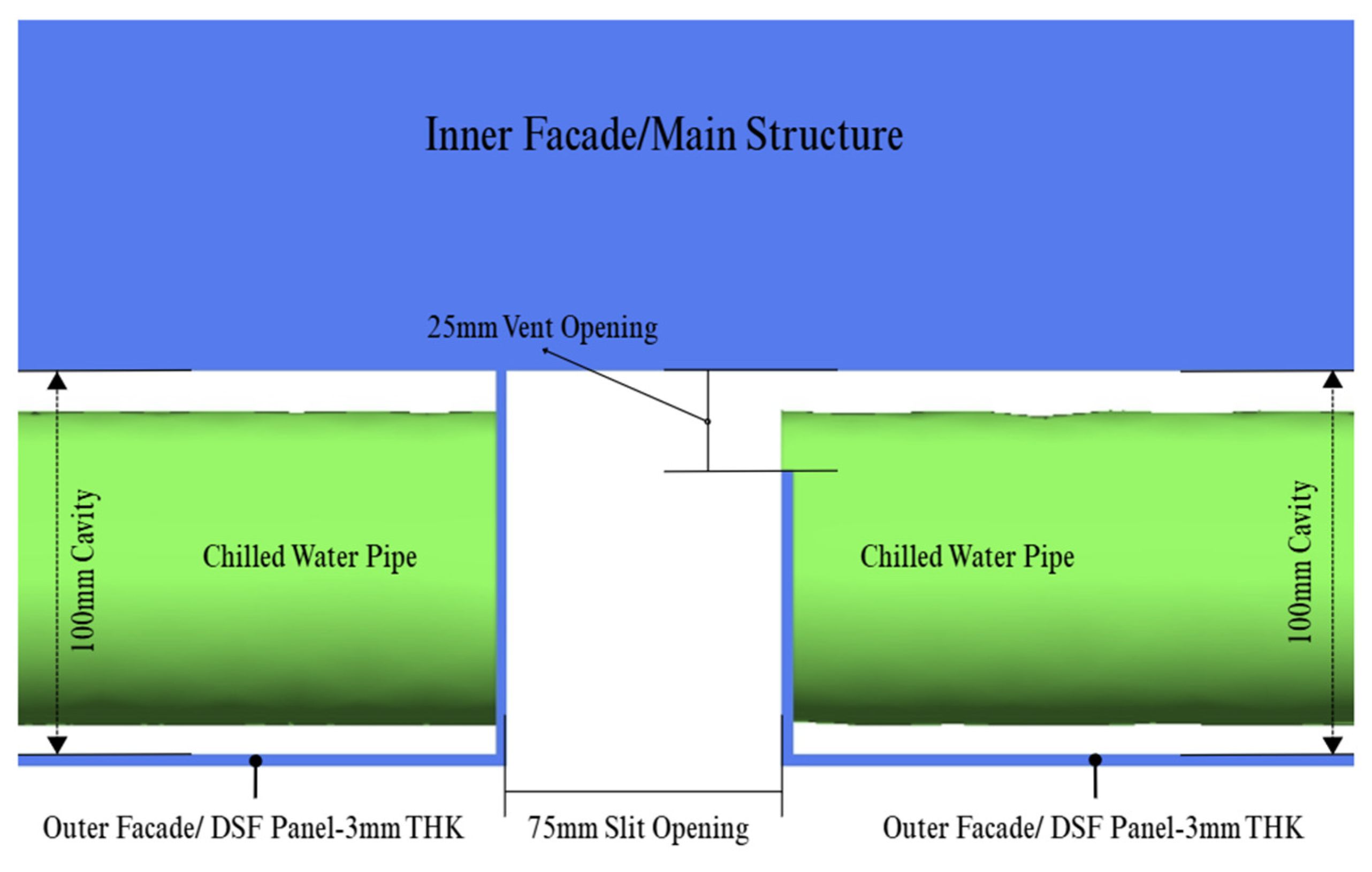
Figure A2.
Zoomed-in isometric view of computational mesh for Model 4, showing the global element distribution on the domain with local refinement near ventilation openings and pipe surfaces.
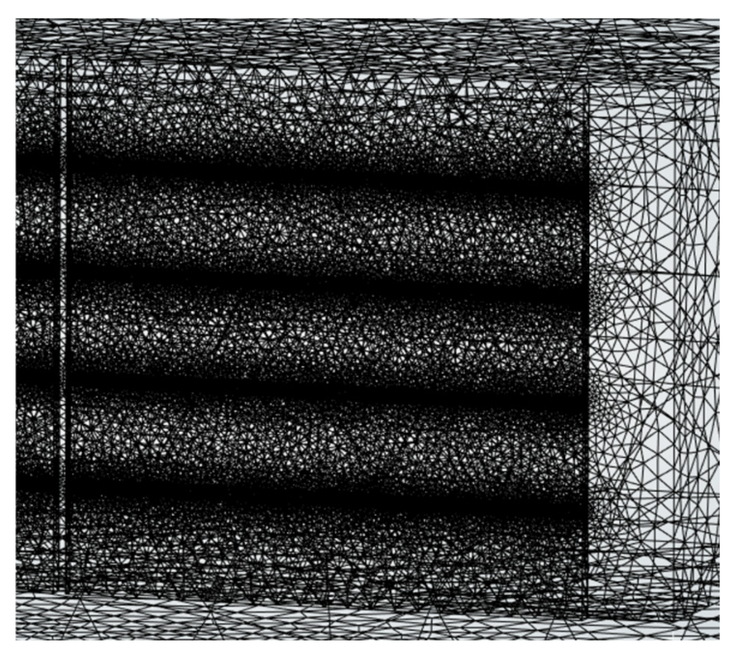
Figure A3.
Front view (left) and sectional view (right) of the Model 4 (M4) computational mesh, showing the refined elements within the narrow 0.10 m cavity and around CHW pipe surfaces.
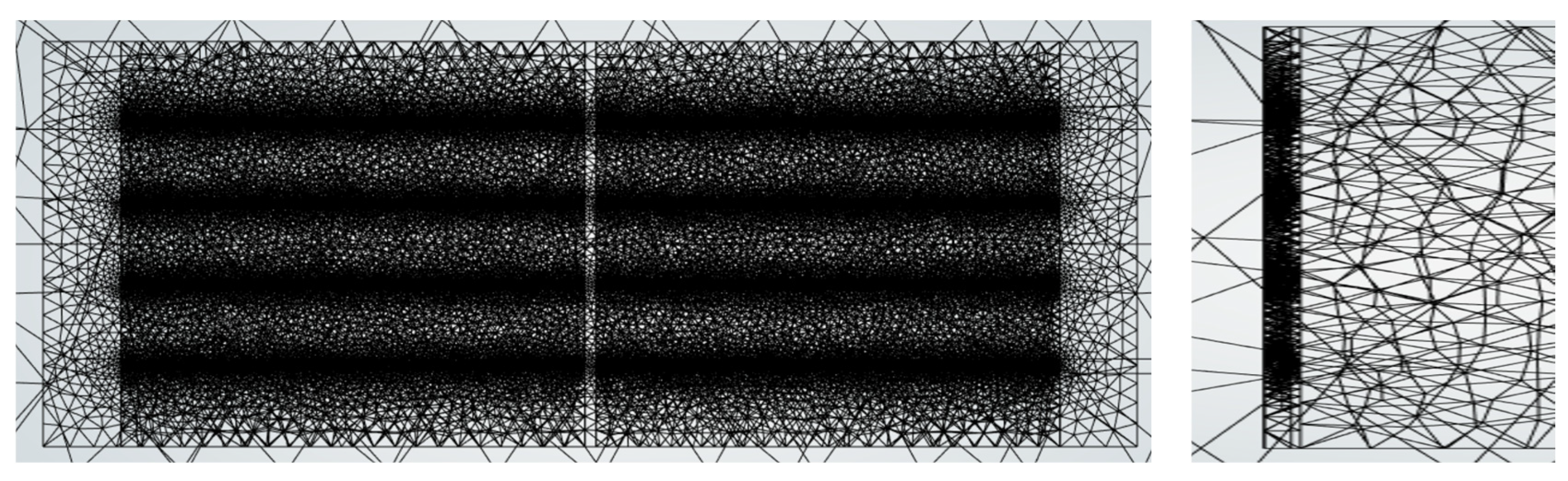
Figure A4.
Zoomed aerial view of the Model 4 slit-inlet mesh, showing the refined tetrahedral elements at the 0.025 m slit opening within the 0.075 m panel-to-panel separation and the inflation layers around the CHW pipes.
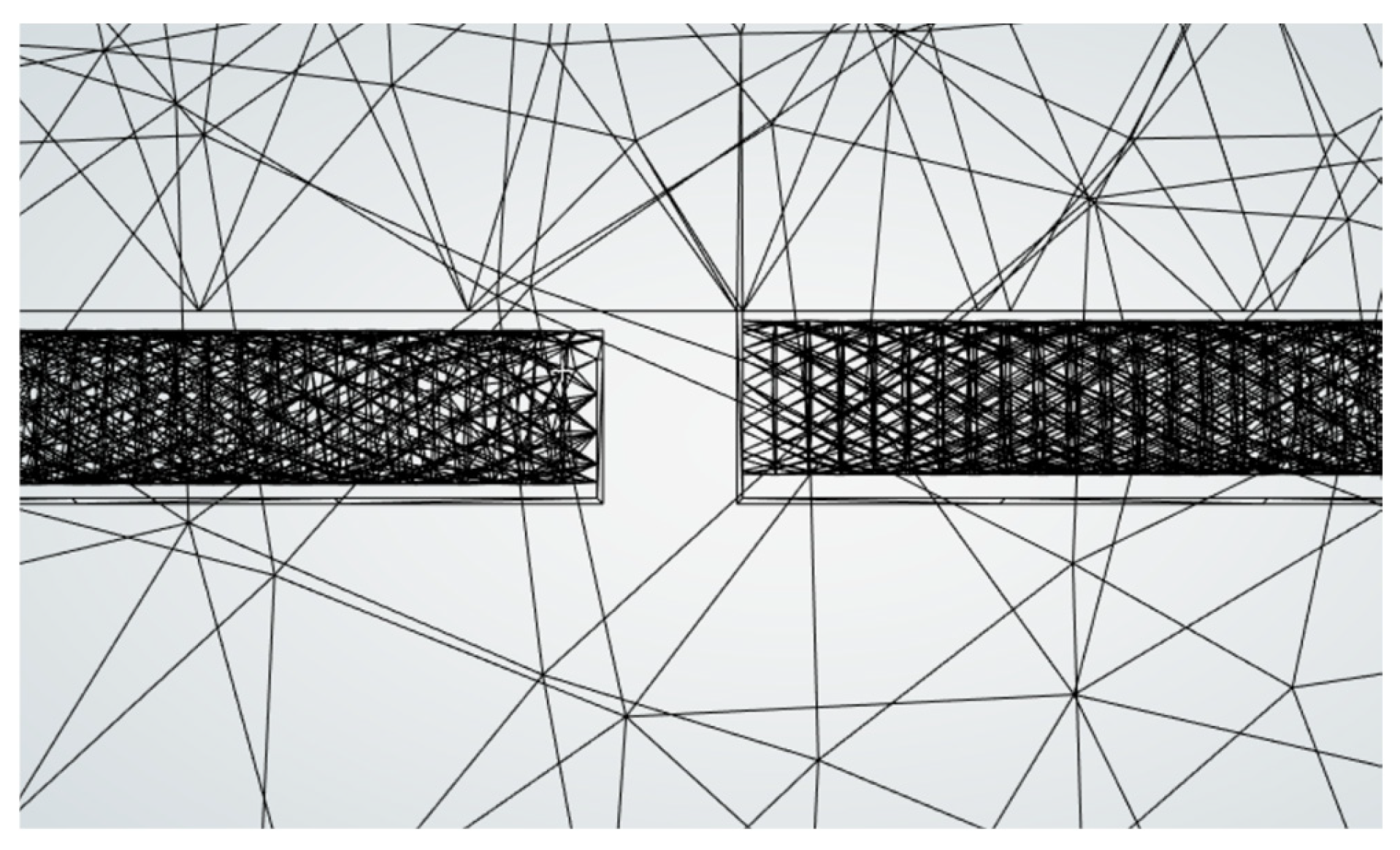
Figure A5.
Streamwise temperature contours for Models 1–4 at the selected vertical section. Models 1 and 2 use a 24–50 °C scale, while Models 3 and 4 use a 10–50 °C scale to show local regions near the 10 °C cooling surfaces. Colour magnitudes should not be compared directly across the two scales.
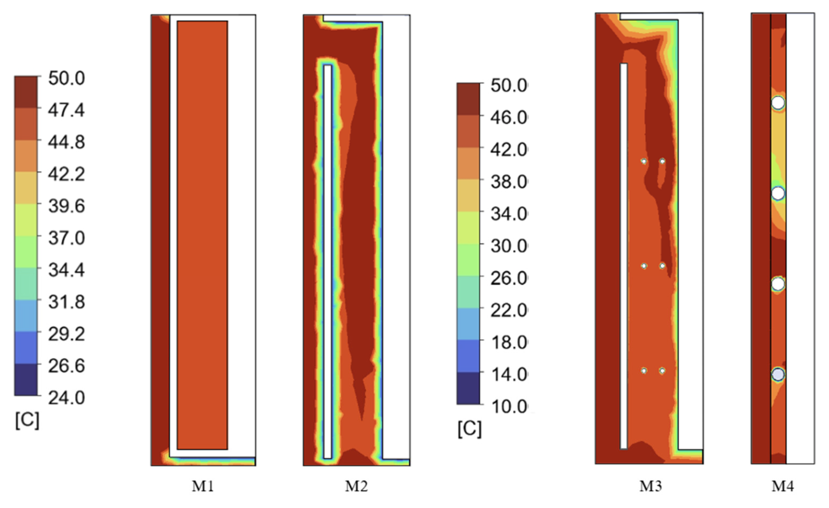
Figure A6.
Aerial temperature contours for Models 1–4 at the selected height. Models 1 and 2 use a 24–50 °C scale, while Models 3 and 4 use a 10–50 °C scale. Colour magnitudes should not be compared directly across the two scales.
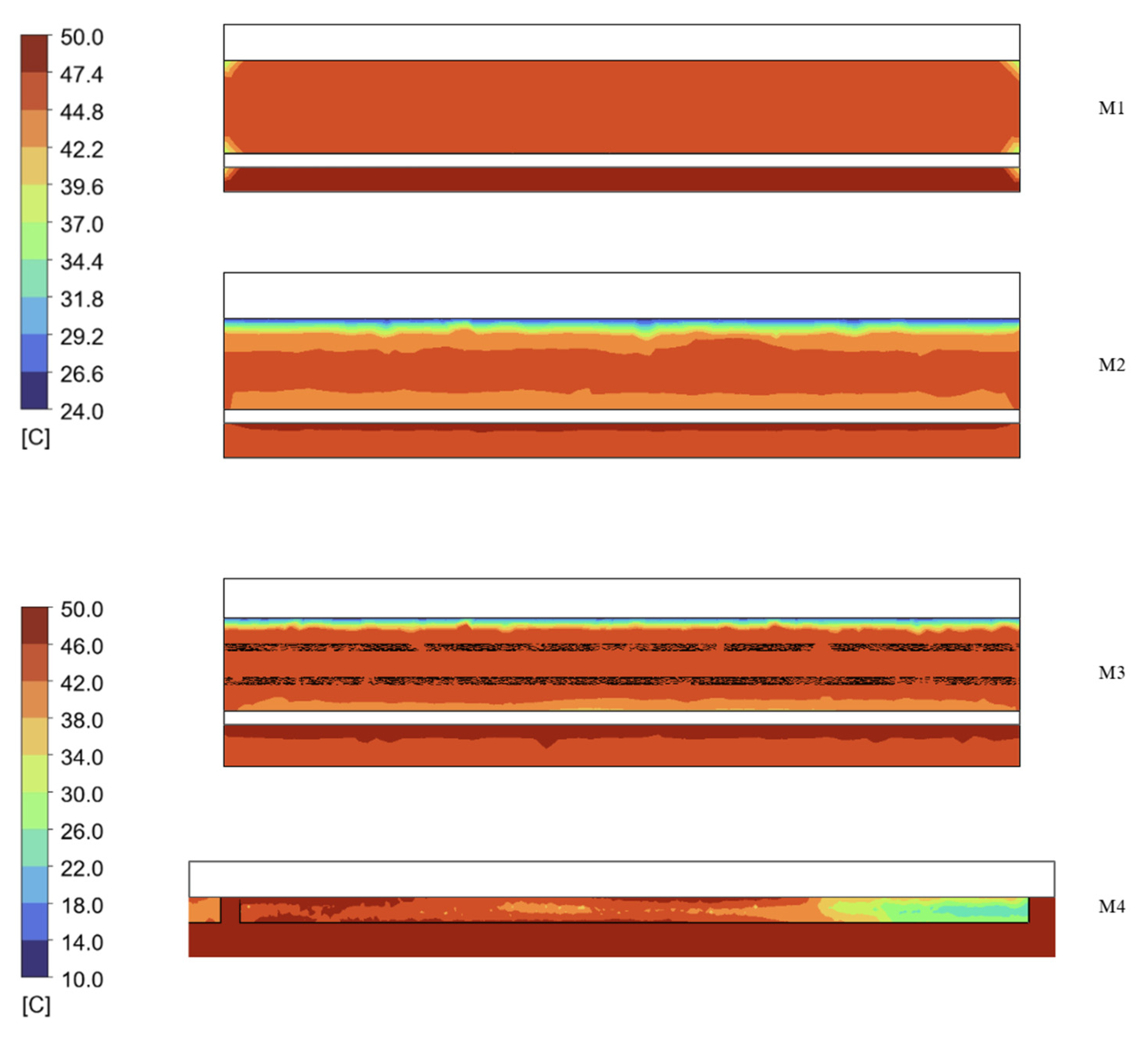
Figure A7.
Streamwise temperature profiles for Models 1–4, extracted from the inner surface of the outer skin to the inner skin face. The probe traverses 100 sampling points.
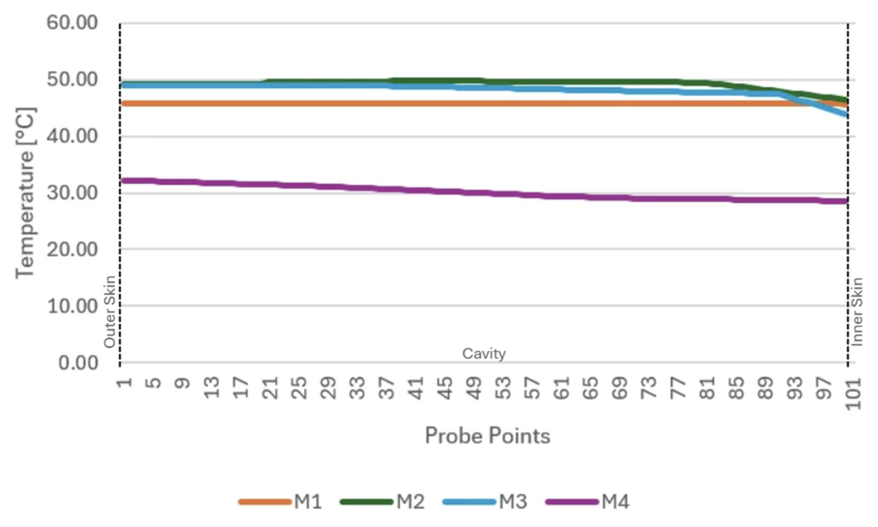
Figure A8.
Vertical temperature profiles for Models 1–4, extracted from the top to the bottom of the cavity at the selected location. Each profile contains 100 normalised sampling points.
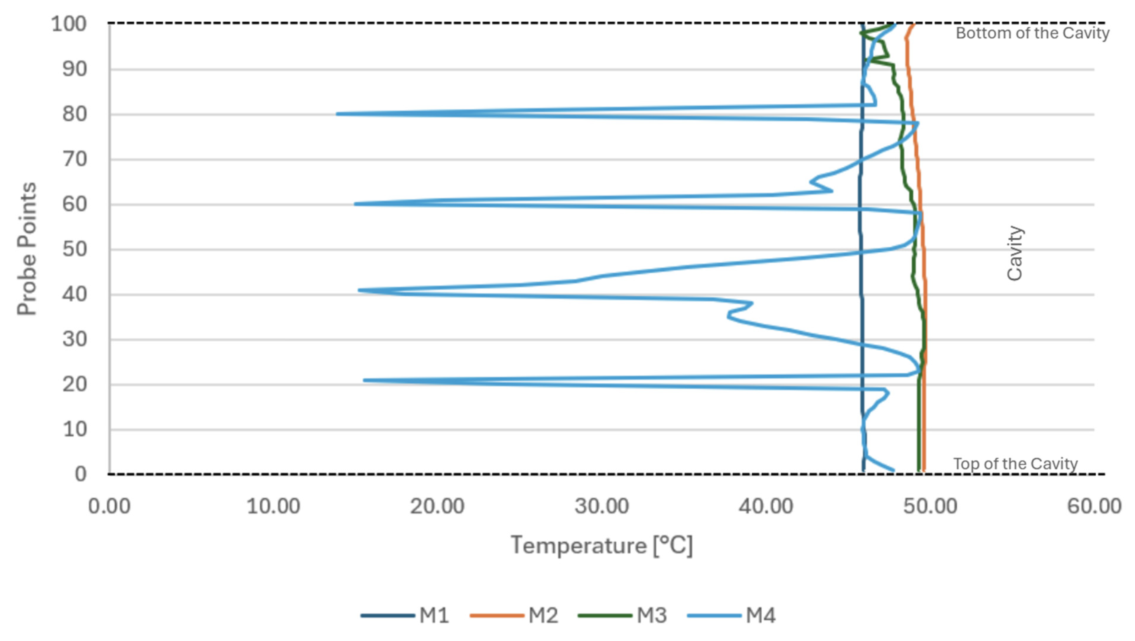
Figure A9.
Zoomed streamwise temperature contour for Model 3, showing the 0.4 m cavity depth with CHW pipe locations and the thermal gradient from the outer façade panel (50 mm) to the inner wall.
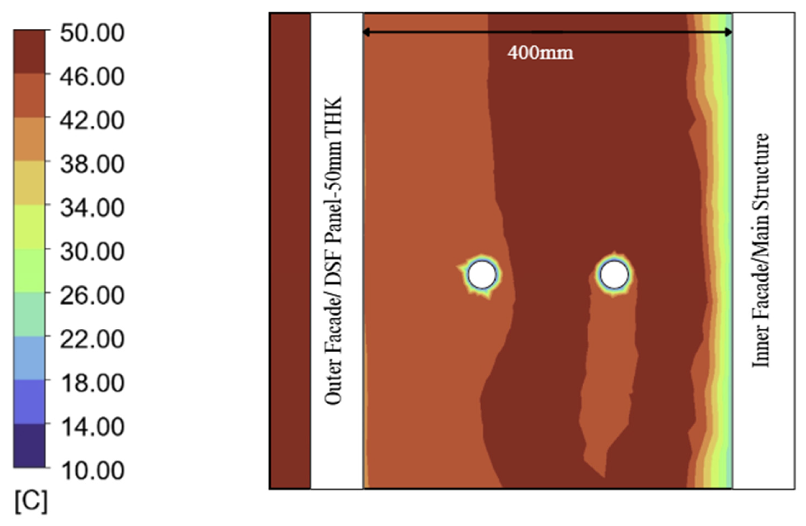
Figure A10.
Zoomed streamwise temperature contour for Model 4, showing the narrow 0.10 m cavity depth with CHW pipe locations and the confined thermal gradient from the aluminium panel (3 mm) to the inner wall.
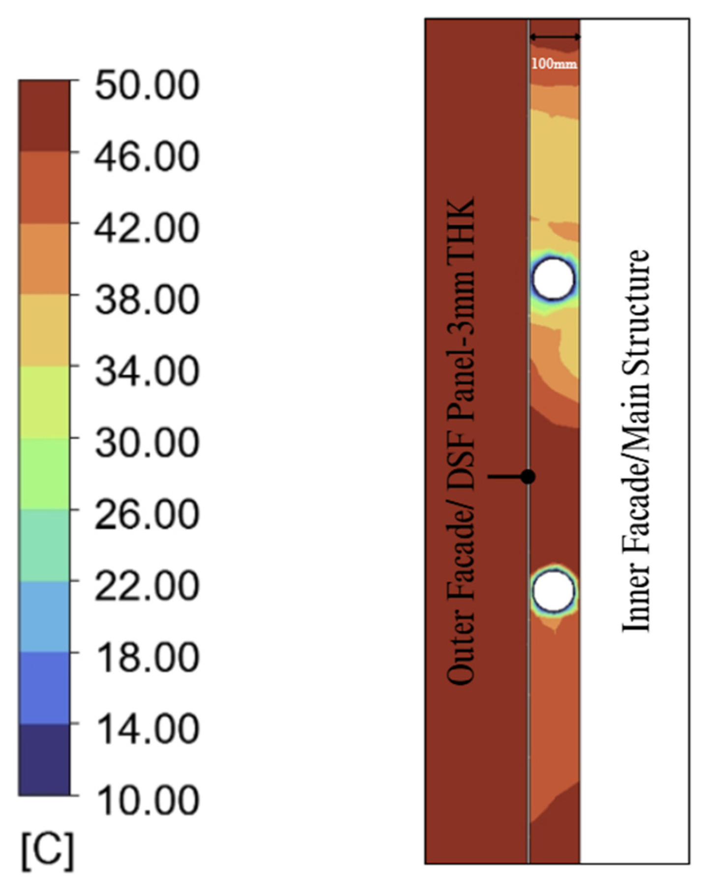
Figure A11.
Streamwise velocity contours for Models 1–4 at the selected vertical section. Independent contour scales are used (M1/M2: 0–7.7 m/s; M3: 0–6.2 m/s; M4: 0–9.3 m/s), so the panels should be compared for spatial pattern rather than colour magnitude.
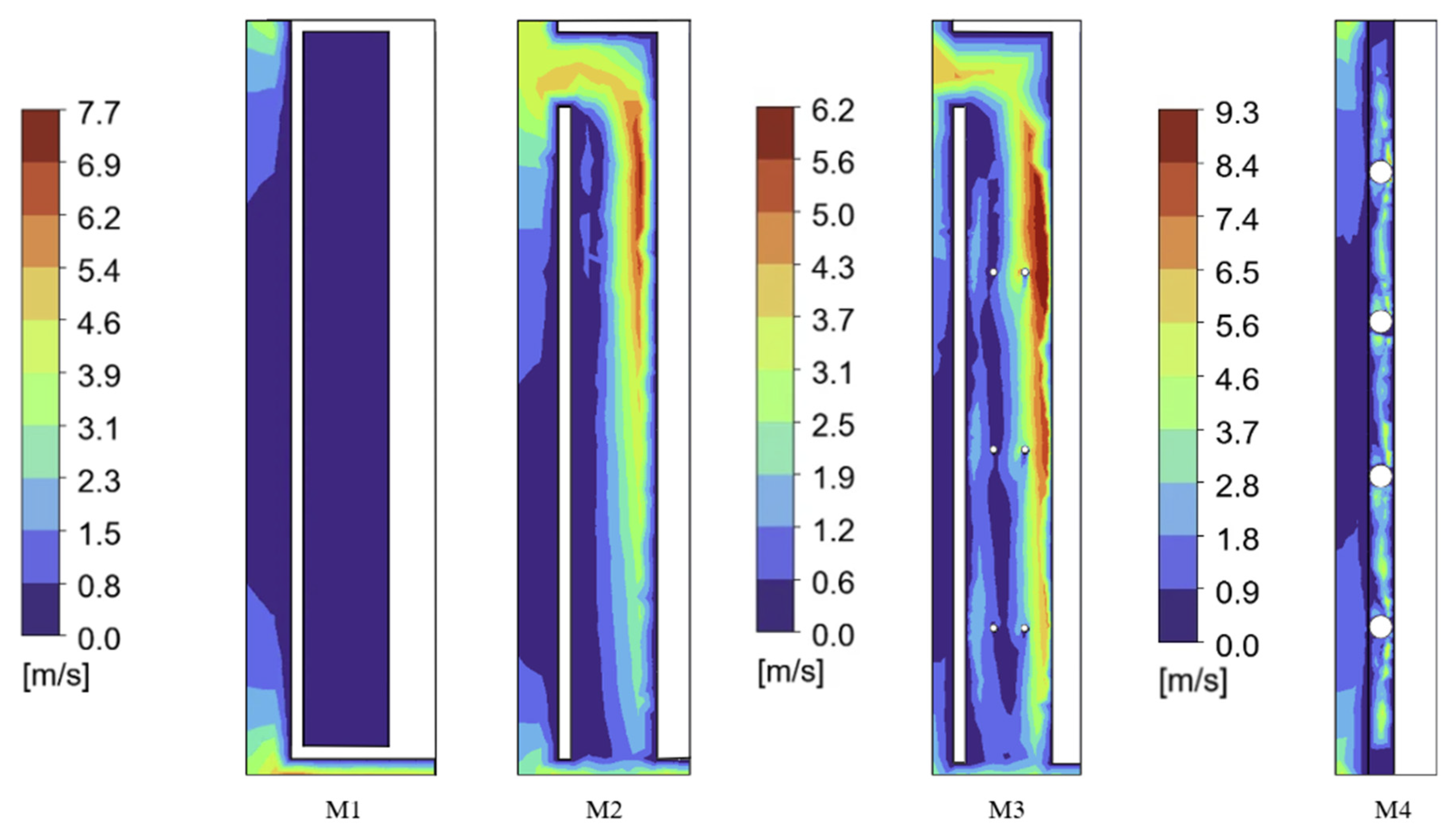
Figure A12.
Aerial velocity contours for Models 1–4 at mid-height. Note: All four models share a common contour scale of 0–6.3 m/s, permitting direct visual comparison of the velocity distribution at the mid-height horizontal plane across all configurations.
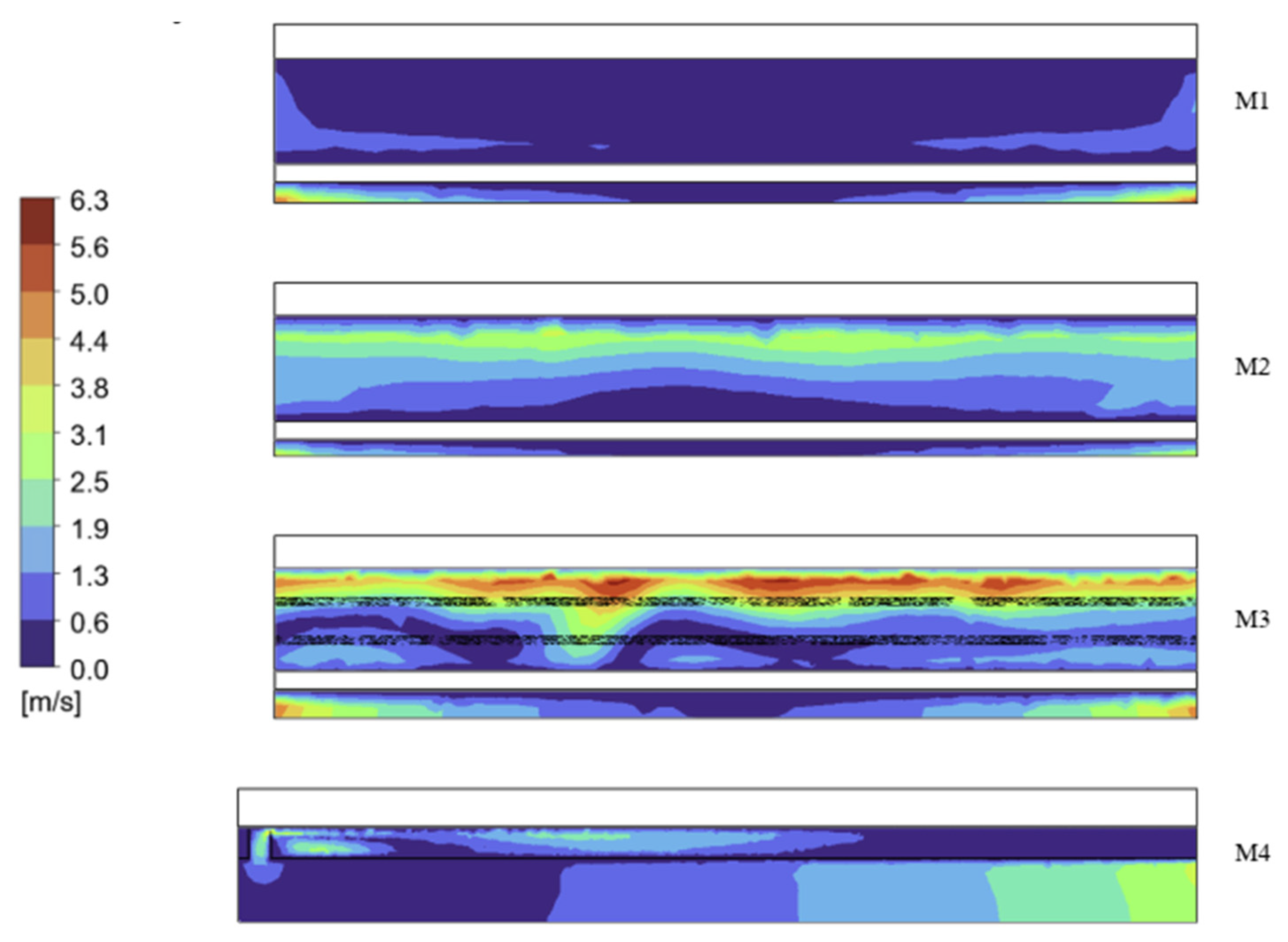
Figure A13.
Streamwise velocity profiles for Models 1–4, extracted from the inner surface of the outer skin to the inner skin face. The probe traverses 100 sampling points.
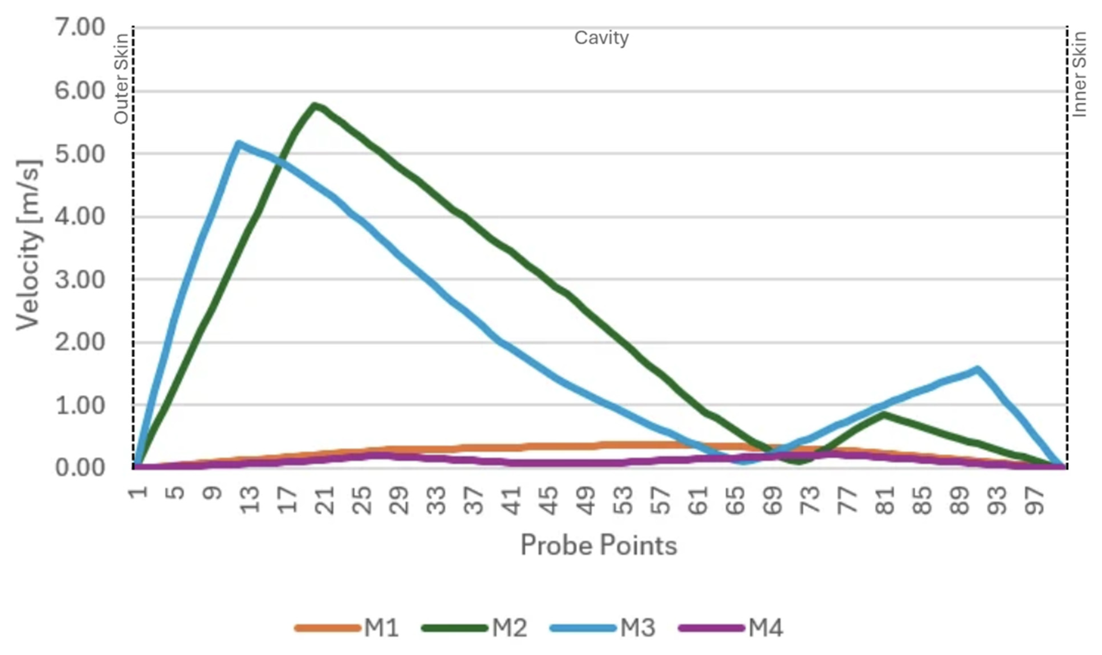
Figure A14.
Vertical velocity profiles for Models 1–4, extracted from the top to the bottom of the cavity at the selected location. Each profile contains 100 normalised sampling points.
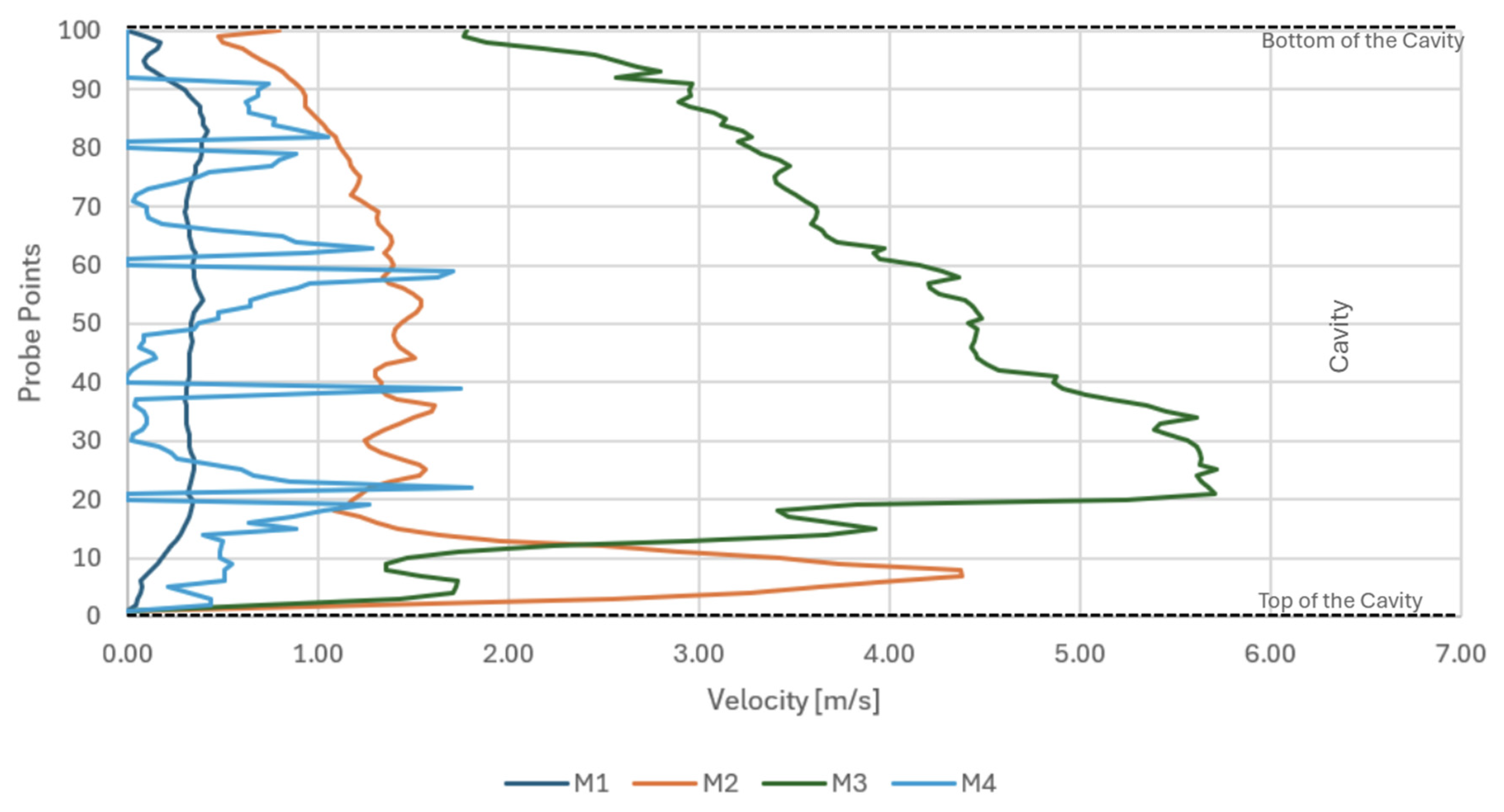
Figure A15.
Zoomed streamwise velocity contour for Model 3, showing flow acceleration through inter-pipe gaps (regions between adjacent cooling-pipe surfaces) and wake deceleration zones within the 0.4 m cavity.
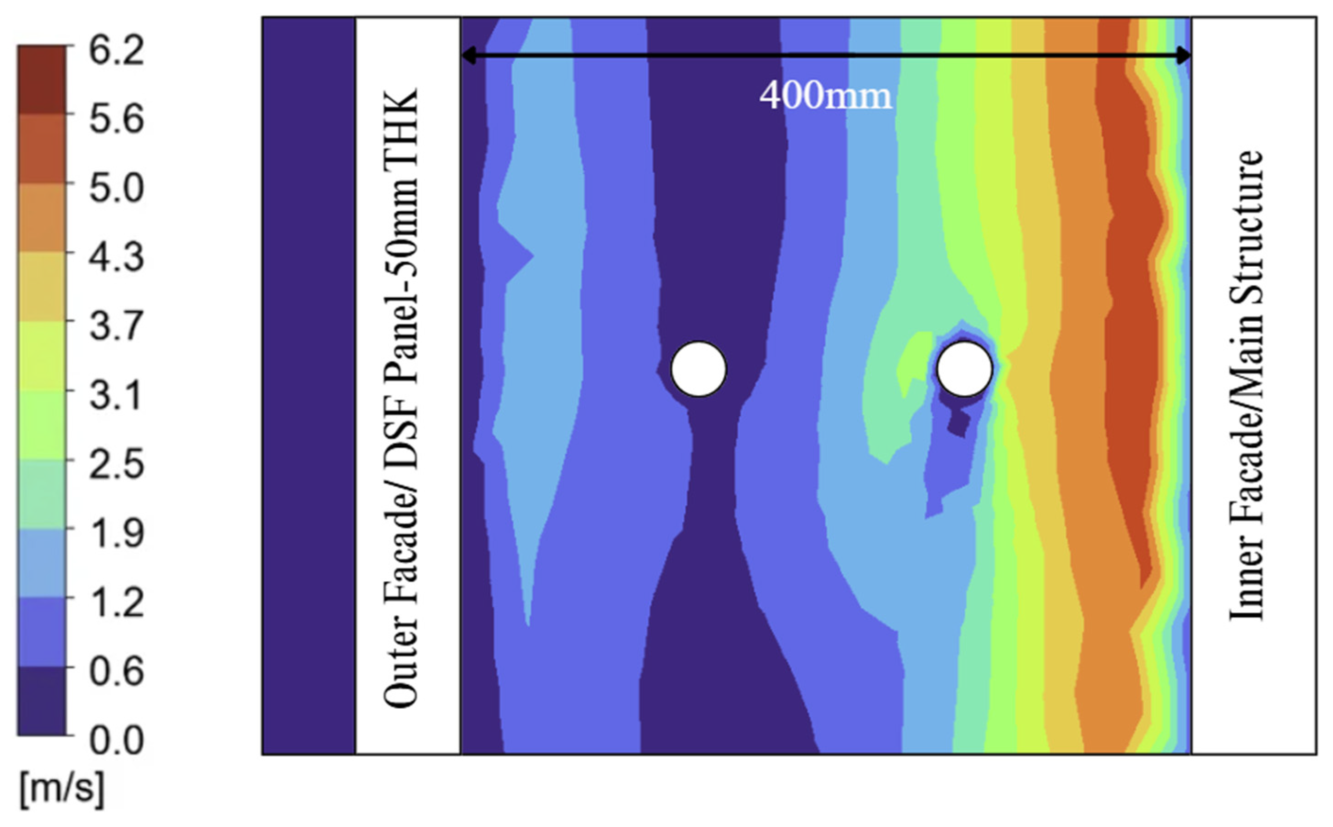
Figure A16.
Zoomed aerial velocity contour for Model 4, showing local acceleration near the slit and lower velocities over parts of the lateral cavity. Maxima differ among slices and line probes; values from independently scaled planes should not be treated as the same pointwise extremum.
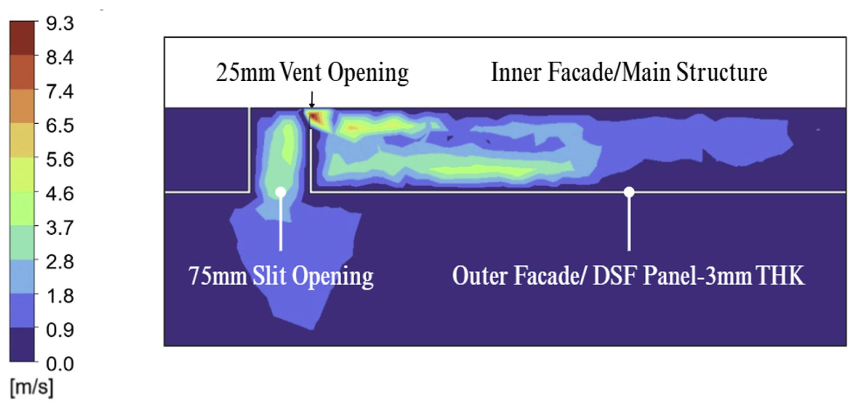
Figure A17.
Streamwise TKE contours for Models 1–4 at the selected vertical section. Each model uses an independently auto-scaled range (M1/M2: 0–2.8 m2/s2; M3: 0–2.6 m2/s2; M4: 0–2.7 m2/s2), so the panels show spatial patterns rather than being directly comparable in colour magnitude.
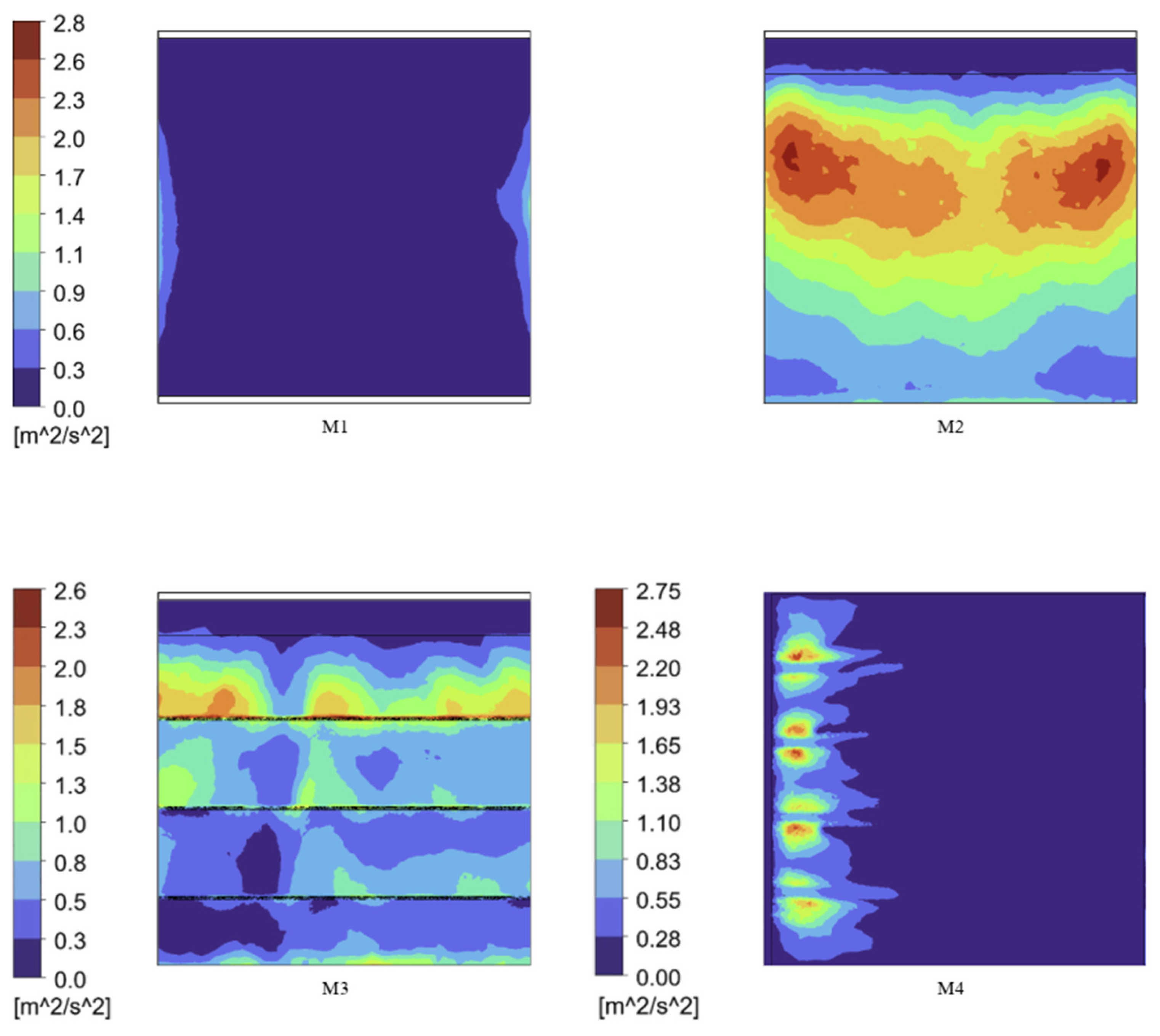
Figure A18.
Aerial TKE contours for Models 1–4 at the selected height. Models 1–3 use a 0–2.2 m2/s2 scale and Model 4 uses a 0–3.5 m2/s2 scale to show a local entry-region peak. Colour magnitudes should not be compared directly across the different scales.
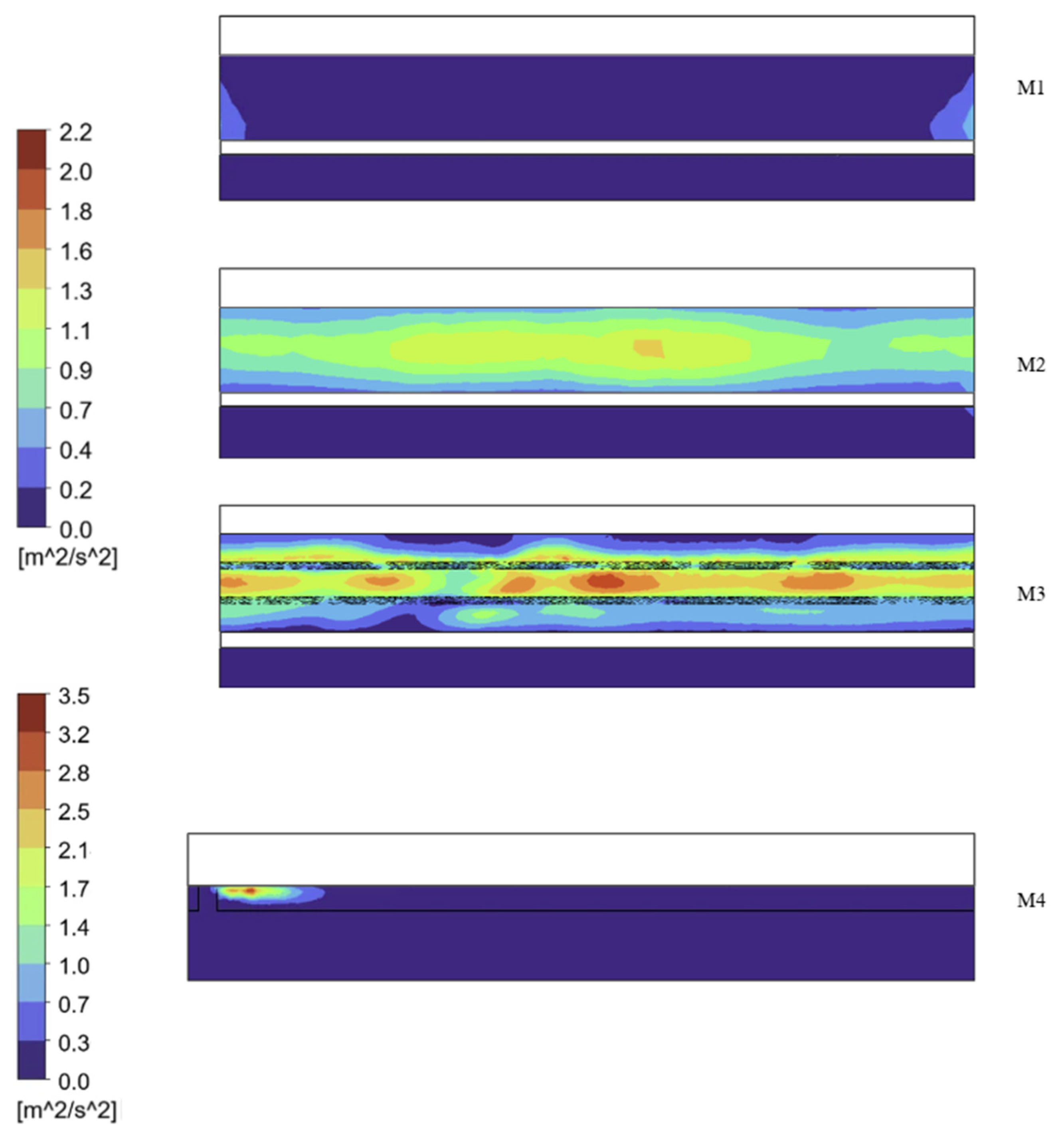
Figure A19.
Streamwise TKE profiles for Models 1–4, extracted from the inner surface of the outer skin to the inner skin face. The probe traverses 100 sampling points.
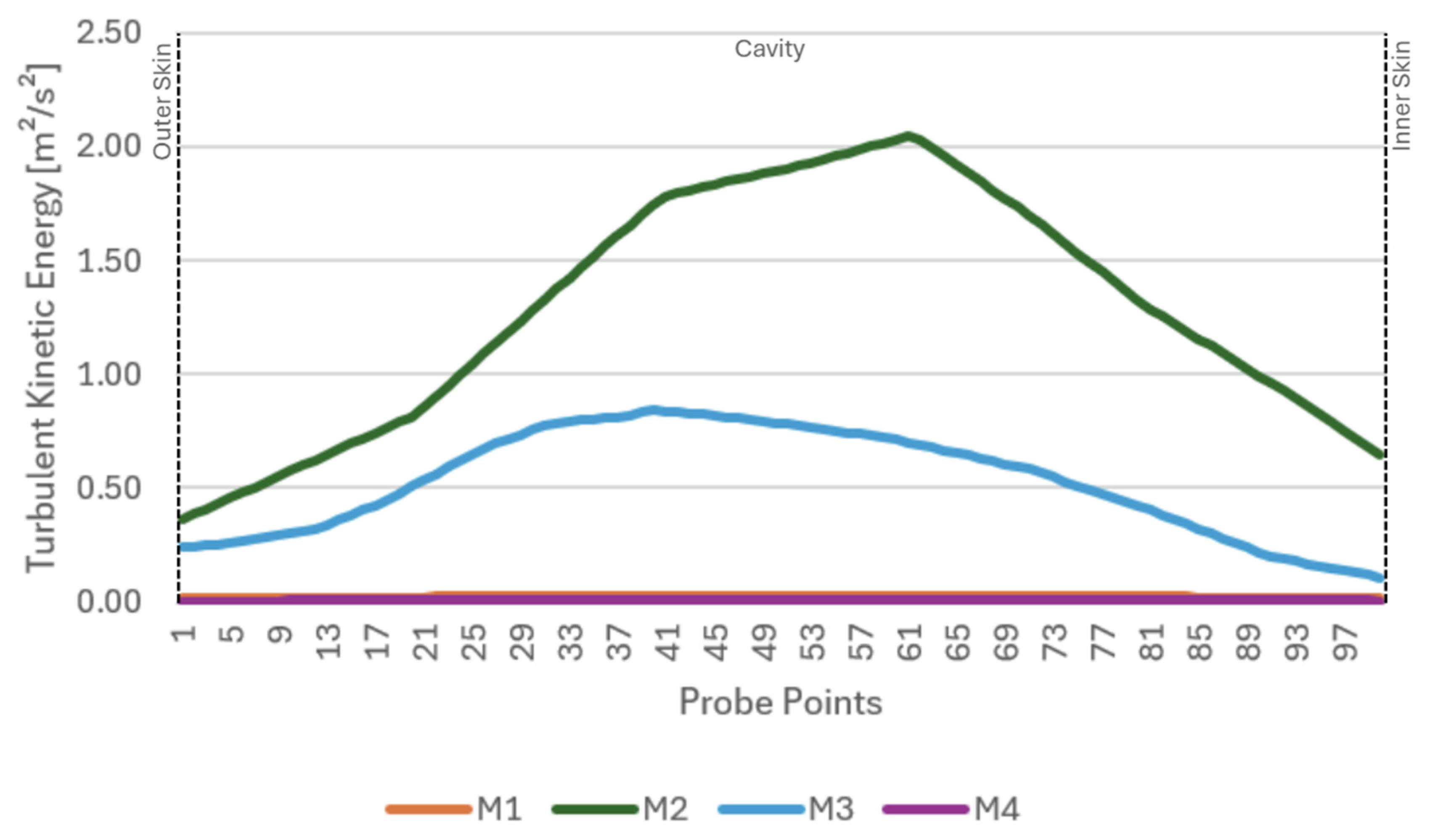
Figure A20.
Vertical TKE profiles for Models 1–4, extracted from the top to the bottom of the cavity at the selected location. Each profile contains 100 normalised sampling points.
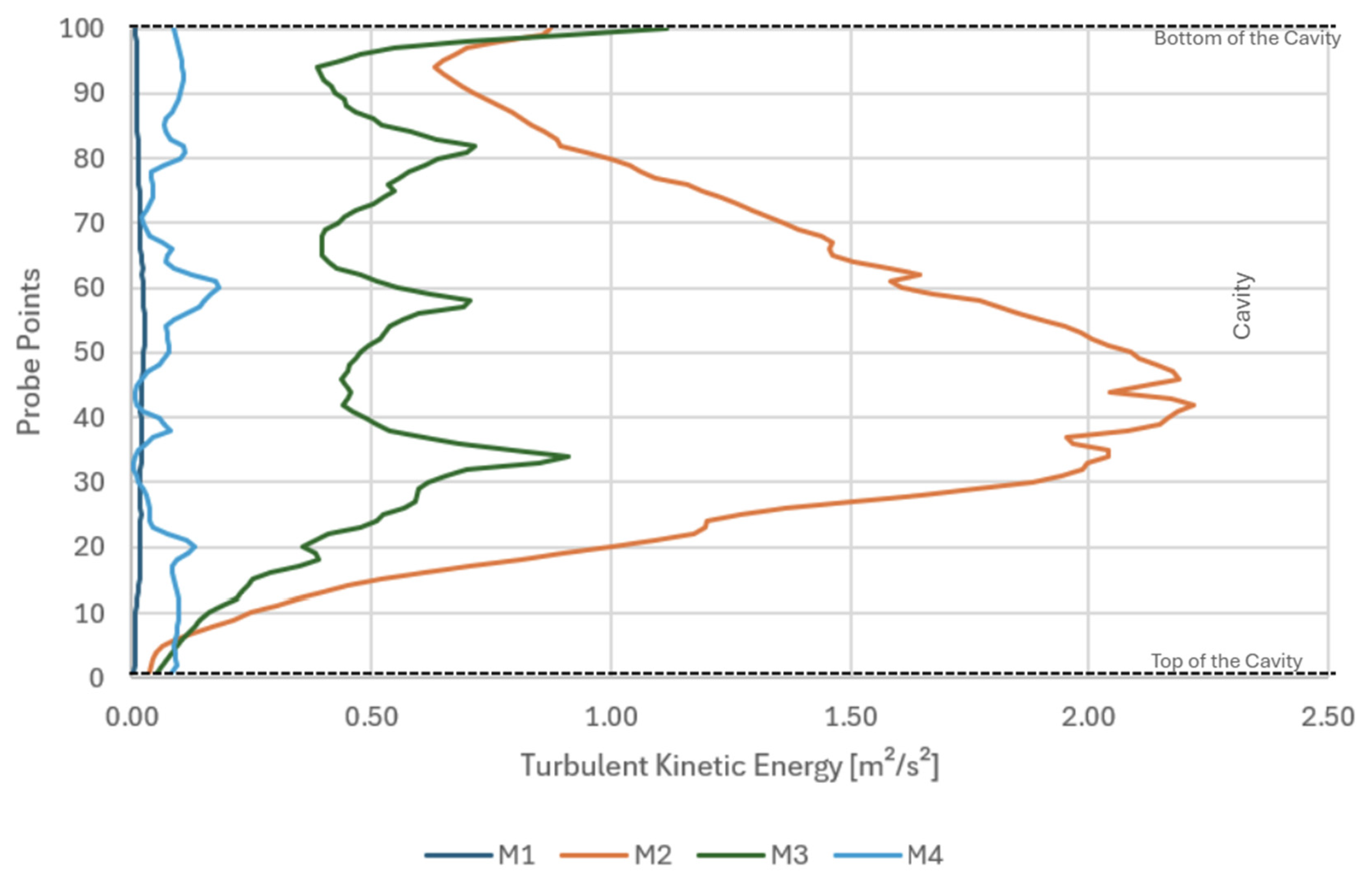
Figure A21.
Zoomed streamwise TKE contour for Model 3, showing pipe-structured turbulence bands with concentrated eddies in the pipe wake regions.
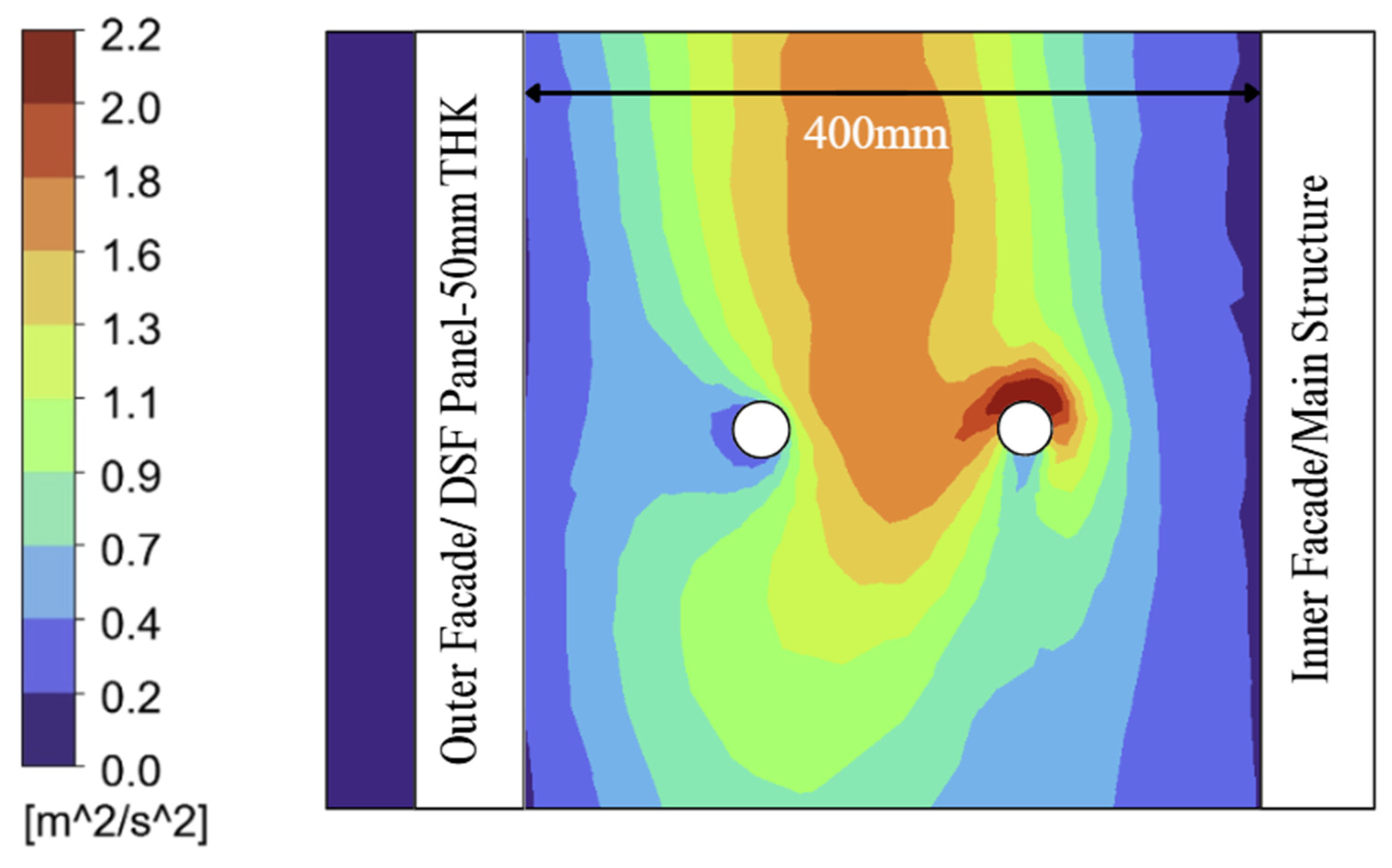
Figure A22.
Zoomed aerial TKE contour for Model 4, showing local modelled TKE peaks near the slit and lower modelled TKE over other portions of the selected plane.
References
- Hamza, N. Double versus single skin facades in hot arid areas. Energy Build. 2008, 40, 240–248. [Google Scholar] [CrossRef] [Scilit]
- United Facade. Façade Engineering Challenges in the Middle East; Technical White Paper; United Facade: Dubai, United Arab Emirates, 2023. [Google Scholar]
- Barbosa, S.; Ip, K. Perspectives of double skin façades for naturally ventilated buildings: A review. Renew. Sustain. Energy Rev. 2014, 40, 1019–1029. [Google Scholar] [CrossRef] [Scilit]
- Ghaffarianhoseini, A.; Ghaffarianhoseini, A.; Berardi, U.; Tookey, J.; Li, D.H.W.; Kariminia, S. Exploring the advantages and challenges of double-skin façades (DSFs). Renew. Sustain. Energy Rev. 2016, 60, 1052–1065. [Google Scholar] [CrossRef] [Scilit]
- Shameri, M.A.; Alghoul, M.A.; Sopian, K.; Zain, M.F.M.; Elayeb, O. Perspectives of double skin façade systems in buildings and energy saving. Renew. Sustain. Energy Rev. 2011, 15, 1468–1475. [Google Scholar] [CrossRef] [Scilit]
- Pomponi, F.; Piroozfar, P.A.E.; Southall, R.; Ashton, P.; Farr, E.R.P. Energy performance of double-skin façades in temperate climates: A systematic review and meta-analysis. Renew. Sustain. Energy Rev. 2016, 54, 1525–1536. [Google Scholar] [CrossRef] [Scilit]
- Zhou, J.; Chen, Y. A review on applying ventilated double-skin façade to buildings in hot-summer and cold-winter zone in China. Renew. Sustain. Energy Rev. 2010, 14, 1321–1328. [Google Scholar] [CrossRef] [Scilit]
- Pelletier, K.; Wood, C.; Calautit, J.; Wu, Y. The viability of double-skin façade systems in the 21st century: A systematic review and meta-analysis of the nexus of factors affecting ventilation and thermal performance, and building integration. Build. Environ. 2023, 228, 109870. [Google Scholar] [CrossRef] [Scilit]
- Wong, P.C.; Prasad, D.; Behnia, M. A new type of double-skin façade configuration for the hot and humid climate. Energy Build. 2008, 40, 1941–1945. [Google Scholar] [CrossRef] [Scilit]
- Aldawoud, A.; Salameh, T.; Ki Kim, Y. Double skin façade: Energy performance in the United Arab Emirates. Energy Sources Part B Econ. Plan. Policy 2021, 16, 387–405. [Google Scholar] [CrossRef] [Scilit]
- Abtar, A.N. A review of the development and applicability of double-skin facades in hot climates. ARO Sci. J. Koya Univ. 2021, 9, 96–106. [Google Scholar] [CrossRef] [Scilit]
- Wang, M.; Peng, J.; Li, N.; Yang, H.; Wang, C.; Li, X.; Lu, T. Optimisation of the double skin facade in hot and humid climates through altering the design parameter combinations. Build. Simul. 2021, 14, 511–521. [Google Scholar] [CrossRef] [Scilit]
- Naddaf, M.S.; Baper, S.Y. The role of double-skin facade configurations in optimizing building energy performance in Erbil city. Sci. Rep. 2023, 13, 8394. [Google Scholar] [CrossRef] [Scilit] [PubMed]
- Saleh, M.J.; Alibaba, H.Z. Design of double skin façade as a sustainable system: The effect of ventilated cavity. Int. J. Archit. Environ. Eng. 2015, 9, 1321–1326. [Google Scholar]
- Manz, H.; Frank, T. Thermal simulation of buildings with double-skin façades. Energy Build. 2005, 37, 1114–1121. [Google Scholar] [CrossRef] [Scilit]
- Gratia, E.; De Herde, A. Optimal operation of a south double-skin facade. Energy Build. 2004, 36, 41–60. [Google Scholar] [CrossRef] [Scilit]
- Pappas, A.; Zhai, Z.J. Numerical investigation on thermal performance and correlations of double skin façade with buoyancy-driven airflow. Energy Build. 2008, 40, 466–475. [Google Scholar] [CrossRef] [Scilit]
- Jiru, T.E.; Haghighat, F. Modeling ventilated double skin façade-A zonal approach. Energy Build. 2008, 40, 1567–1576. [Google Scholar] [CrossRef] [Scilit]
- Larsen, T.S.; Nikolopoulos, N.; Nikolopoulos, A.; Skotte, K.S.; Olesen, B.W. CFD modelling of a double-skin façade in practice. Build. Simul. 2015, 8, 237–248. [Google Scholar]
- Coussirat, M.; Guardo, A.; Jou, E.; Egusquiza, E.; Cuerva, E.; Alavedra, P. Performance and influence of numerical sub-models on the CFD simulation of free and forced convection in double-glazed ventilated façades. Energy Build. 2008, 40, 1781–1789. [Google Scholar] [CrossRef] [Scilit]
- Guardo, A.; Coussirat, M.; Valero, M.; Egusquiza, E.; Alavedra, P. CFD assessment of the performance of lateral ventilation in double-glazed façades in Mediterranean climates. Energy Build. 2011, 43, 2539–2547. [Google Scholar] [CrossRef] [Scilit]
- Valentín, D.; Guardo, A.; Egusquiza, E.; Valero, M.; Alavedra, P. Use of Coandă nozzles for double glazed façades forced ventilation. Energy Build. 2013, 62, 605–614. [Google Scholar] [CrossRef] [Scilit]
- Melgaard, S.P.; Nikolaisson, I.T.; Zhang, C.; Johra, H.; Larsen, O.K. Double-skin façade simulation with computational fluid dynamics: A review of simulation trends, validation methods and research gaps. Build. Simul. 2023, 16, 2307–2331. [Google Scholar] [CrossRef] [Scilit]
- Ahmadi, J.; Mahdavinejad, M.; Larsen, O.K.; Zhang, C. Evaluating the different boundary conditions to simulate airflow and heat transfer in double-skin facade. Build. Simul. 2022, 15, 799–815. [Google Scholar] [CrossRef] [Scilit]
- Catto Lucchino, E.; Gelesz, A.; Skeie, K.; Goia, F.; Favoino, F. Modelling double skin façades (DSFs) in whole-building energy simulation tools: Validation and inter-software comparison of a mechanically ventilated single-story DSF. Build. Environ. 2021, 199, 107906. [Google Scholar] [CrossRef] [Scilit]
- Yang, X.; He, J.; Zhang, Y.; Huang, G.; Wang, J.; Liao, L. Experimental investigation on cooling performance of water spray window. Buildings 2024, 14, 1687. [Google Scholar] [CrossRef] [Scilit]
- Shen, C.; Li, X. Thermal performance of double skin façade with built-in pipes utilizing evaporative cooling water in cooling season. Sol. Energy 2016, 137, 55–65. [Google Scholar] [CrossRef] [Scilit]
- Hedayat, Z.; Samkhaniani, N.; Belmans, B.; Ayatollahi, M.H.; Wouters, I.; Descamps, F. Energy performance analysis of solar-wind catchers under hot and dry climatic condition in Iran-Yazd. J. Sol. Energy Res. 2017, 2, 13–19. [Google Scholar] [CrossRef] [Scilit]
- de Gracia, A.; Navarro, L.; Castell, A.; Cabeza, L.F. Energy performance of a ventilated double skin facade with PCM under different climates. Energy Build. 2015, 91, 37–42. [Google Scholar] [CrossRef] [Scilit]
- Li, Y.; Darkwa, J.; Kokogiannakis, G. Heat transfer analysis of an integrated double skin facade and phase change material blind system. Build. Environ. 2017, 125, 111–121. [Google Scholar] [CrossRef] [Scilit]
- Li, Y.; He, W.; Tao, W.; Yang, C.; Li, Y.; Darkwa, J. Impacts of design parameters on the thermal performance of a macro-encapsulated phase-change-material blind integrated in a double-skin façade system. Energies 2025, 18, 3326. [Google Scholar] [CrossRef] [Scilit]
- Sotelo-Salas, C.; Pozo, C.E.; Esparza-López, C.J. Thermal assessment of spray evaporative cooling in opaque double skin facade for cooling load reduction in hot arid climate. J. Build. Eng. 2021, 38, 102156. [Google Scholar] [CrossRef] [Scilit]
- Calautit, J.K.; Hughes, B.R.; Shahzad, S.S. CFD and wind tunnel study of the performance of a uni-directional wind catcher with heat transfer devices. Renew. Energy 2015, 83, 85–99. [Google Scholar] [CrossRef] [Scilit]
- Muhammed, S.; Chaudhry, H.N.; Santiago, I.M.C. An analytical study of horizontal adaptations of vernacular Barjeel (windcatcher) in the desert architecture of the Gulf region. Architecture 2026, 6, 43. [Google Scholar] [CrossRef] [Scilit]
- Khan, A.H.; Islam, M.S.; Sazzad, I.U. Calibration of k-ε turbulence model for thermal-hydraulic analyses in rib-roughened narrow rectangular channels using genetic algorithm. SN Appl. Sci. 2021, 3, 678. [Google Scholar] [CrossRef] [Scilit]

Disclaimer/Publisher’s Note: The statements, opinions and data contained in all publications are solely those of the individual author(s) and contributor(s) and not of MDPI and/or the editor(s). MDPI and/or the editor(s) disclaim responsibility for any injury to people or property resulting from any ideas, methods, instructions or products referred to in the content. |
© 2026 by the authors. Licensee MDPI, Basel, Switzerland. This article is an open access article distributed under the terms and conditions of the Creative Commons Attribution (CC BY) license.