The Influence of Dynamic Soil–Structure Interaction on a Damage Detection Algorithm

Abstract

This study evaluates the impact of Dynamic Soil–Structure Interaction (DSSI) on the efficiency of an algorithm based on the existing literature on Vibration-Based Structural Health Monitoring (VBSHM). The algorithm is designed for Level 3 detection, that is, to accurately estimate the presence, location in height, and extent of structural damage simultaneously. Using computer simulations of a hypothetical two-dimensional six-story symmetrical reinforced concrete building, the study analyzes the algorithm’s performance under increasing soil flexibility. Efficiency is measured through four key metrics: the number of false positives and negatives, a weighted stress index, the iterations required for damage intensity estimation, and the accuracy of the identified versus simulated stiffness reduction. Results indicate that the algorithm remains effective even when input motions correspond to actual soft-soil ambient vibration recordings modified by kinematic DSSI effects, despite frequency contents differing from white-noise conditions. Conversely, inertial DSSI negatively impacts performance, leading the VBSHM algorithm to underestimate damage as soil deposits become softer.

1. Introduction

Currently, various techniques exist for Structural Health Monitoring (SHM); one approach, driven by the increasing market accessibility of high-precision sensors, is Vibration-Based Structural Health Monitoring (VBSHM). In VBSHM, changes in a structure’s dynamic response are captured through sensor networks. The primary objective of vibration monitoring is to identify damage across four progressive levels [1]: Level 1, detecting its presence; Level 2, identifying its location; Level 3, quantifying its extent; and Level 4, predicting the remaining service life or expected consequences of the damage.

The fundamental principle of VBSHM is that a system’s dynamic characteristics are direct functions of its physical properties. Consequently, it is assumed that any degradation in physical integrity will manifest as a detectable change in dynamic response, enabling damage identification. According to Doebling et al. [2], vibration-based damage detection can be achieved by analyzing several parameters, including shifts in natural frequencies, mode shape variations, and changes in flexibility coefficients, among others.

As sensors become more commercially accessible, a growing number of buildings in Mexico City have been instrumented, particularly those situated in soft-soil conditions. Given that the primary goal of any VBSHM system is to provide a reliable framework for structural health assessment, it is crucial to investigate the potential limitations of existing VBSHM techniques when applied to structures on highly flexible soils.

While VBSHM is a growing field, only a limited number of studies specifically address how soil flexibility affects the accuracy of damage identification [3,4], and investigations into its impact on damage-extent estimates (Level 3) are even rarer. Several studies on VBSHM [5,6,7,8,9] typically assume, either explicitly or implicitly, a fixed-base condition by neglecting the changes in frequency content induced by the soil deposit, the wave diffractions generated at the foundation, and the overall system translation and rocking caused by inertial interaction. By emphasizing the substantial research gap between VBSHM and soil–structure interaction, we underscore both the relevance and the necessity of the present study.

When determining a system’s dynamic properties experimentally, it is essential to recognize that the structure is coupled with both its foundation and the underlying soil. Consequently, the recorded response encompasses more than just the fixed-base structural behavior. As demonstrated by Stewart and Fenves [10], the captured data integrates, in varying degrees, the dynamics of the soil deposit, the translational and rotational components of the foundation, and the inherent mechanical properties of the superstructure.

In damage identification, it is critical to decouple the fixed-base structural response from the total response of the soil–foundation–structure (SFS) system. Furthermore, it is essential to determine the potential inaccuracies that arise when a VBSHM algorithm is applied without accounting for DSSI effects. Consequently, the primary objective of this research is to evaluate the impact of soft-soil DSSI on the performance of a VBSHM-based algorithm. As a first approach, this study will only focus specifically on mid-rise reinforced concrete moment-resisting frames (MRFs).

As stated by Wolf [11], Dynamic Soil–Structure Interaction (DSSI) becomes more pronounced as soil flexibility increases and the superstructure becomes stiffer. In contrast, these effects are significantly reduced when a flexible structure is situated on a stiff soil deposit. Incorporating soft-soil conditions into the dynamic model increases the overall system flexibility, thereby reducing the fundamental frequency that is lower than that of a fixed-base system. This frequency shift depends on the relative stiffness between the soil and the structure. Furthermore, the vibrational mode shapes are also modified [12]; specifically, foundation rocking and base translation alter the response, with these effects being particularly evident in the upper stories of the structure.

Luco et al. [13] pointed out that ignoring the effects of DSSI remains a common practice. However, adopting the hypothesis that structural dynamic response is unaffected by the soil and foundation can lead to significant engineering errors. In such cases, the modal frequencies and energy dissipation characteristics of the complete soil–foundation–structure (SFS) system may be misinterpreted as inherent properties of the superstructure alone.

In the same vein, Trifunac and Ebrahimian [14] emphasize that DSSI is an inherent component of a building’s dynamic response. They state that “for reliable structural health monitoring, and in general, for correct structural model calibration, it is essential to monitor the fixed-base building frequency independently from the soil–structure system frequency”.

In the Mexican context, Murià-Vila et al. [15] analyzed the seismic response of an instrumented building, demonstrating the critical importance of accounting for DSSI. Their findings revealed that for structures located in the soft-soil conditions of Mexico City, the interaction effects can result in a fourfold reduction in the fixed-base natural frequency.

DSSI significantly alters a system’s dynamic properties and structural behavior [16,17,18]. Consequently, this phenomenon is expected to impact VBSHM algorithms, which rely on these properties as primary inputs. If coupled parameters—rather than those intrinsic to the superstructure—are used for damage detection, the resulting estimations may be inaccurate or misleading, potentially leading to erroneous assessments of structural integrity.

A significant research gap exists regarding damage identification under DSSI conditions. These effects are particularly critical for stiff structures situated on soft-soil deposits. This specific combination of properties is characteristic of numerous low- to mid-rise buildings located in the lake-bed zone of Mexico City. Consequently, as the implementation of VBSHM becomes increasingly common in this region, investigating these interaction effects is essential to ensure the reliability of structural assessments.

2. Damage Detection Algorithm

Prior to exploring the effects of DSSI on damage detection, a robust fixed-base VBSHM algorithm based on existing well-established techniques was validated. The objective of the proposed algorithm is to achieve Level 3 detection [1], which entails the simultaneous and accurate estimation of the presence, location, and severity of structural damage. While no innovations are introduced to the individual VBSHM techniques, the main contribution of this research is the assessment of the performance of well-established methods under DSSI conditions. Following the initial validation on the fixed-base case, the algorithm’s efficiency was systematically analyzed under the influence of progressive soft-soil DSSI conditions.

The proposed methodology utilizes vibration recordings in two distinct stages: a baseline (undamaged) state and a subsequent damaged state. System frequencies and mode shapes are extracted using the time-domain Eigensystem Realization Algorithm (ERA) [19]. The ERA is fed with the system’s Impulse Response Function (IRF), which is derived by taking the Inverse Fourier Transform (IFT) of the Frequency Response Function (FRF), computed from the frequency-domain analysis of the acceleration recordings.

Within the ERA framework, the system’s impulse response (Markov Parameters) is organized into the Hankel data matrices, $H\left(0\right)$ and $H\left(1\right)$. A Singular Value Decomposition (SVD) is then performed on $H\left(0\right)$, followed by a model reduction retaining only a specific number of singular values. This process yields a discrete-time realization ($\widehat{A}$ denotes estimated variables) of the true system matrix, $A$, as follows:

$$H\left(0\right)=R_n{\Sigma }_n{S}_n^T$$

(1)

$$\left[\widehat{A}\right]=\left[{\Sigma }_n^{-1/2}{R}_n^T\right] H\left(1\right) \left[S_n{\Sigma }_n^{-1/2}\right]$$

(2)

where ${\Sigma }_n$ is a matrix with the n-retained singular values, $R_n$ is a matrix with the left singular vectors and $S_n$ is the matrix of the right singular vectors. After the realization, the identified system matrix was taken back into the continuous-time domain using the sampling Δt time-step as:

$$\left[{\widehat{A}}_c\right]={\displaystyle \frac{1}{\Delta t}}\ln \left[\widehat{A}\right]$$

(3)

Later, the system frequencies, damping ratios and mode shapes are obtained from the eigen solution of the ${\widehat{A}}_c$ matrix, where the identified complex-conjugate $s_n$ eigenvalues (poles) are in the form

$$s_n,s_n^{*}=-\xi {\omega }_n\pm \mathrm{i} {\omega }_d$$

(4)

In Equation (4), ξ is the modal damping ratio, ${\omega }_n$ the system modal circular frequency (rad/s), i the imaginary unit equal to $\sqrt{-1}$ and ${\omega }_d$ the damped system mode circular frequency (rad/s). As shown above, the system poles $s_n$ include modal parameters such as frequencies and damping, such that given the system poles, the frequencies and damping ratios can be calculated as

$${\omega }_n=\left|s_n\right|$$

(5)

$$\xi ={\displaystyle \frac{\mathrm{Real}\left(s_n\right)}{\left|s_n\right|}}$$

(6)

In the same way as the poles are related to frequencies and damping, it can be shown that the eigenvectors of ${\widehat{A}}_c$ are in fact the mode shapes of the system. When complex values of eigenvectors were calculated, a real-plane projection was taken as the system mode shape.

Once the modal properties (frequencies and mode shapes) of the system were identified, the damage identification at Level 1 and 2 was performed by using Damage Location Vectors (DLV) [20]. Under the DLV technique, an SVD is performed on the flexibility change matrix ${\left[f\right]}_{\Delta }$

$${\left[f\right]}_{\Delta }={\left[f\right]}_d-{\left[f\right]}_u$$

(7)

$${\left[f\right]}_{\Delta }=\left[U\right]\left[\Sigma \right]{\left[V\right]}^T$$

(8)

$${\left[f\right]}_{\Delta }=\left[\begin{array}{cc}{U}_1& U_0\end{array}\right]\left[\begin{array}{cc}{S}_1& 0\\ 0& 0\end{array}\right]{\left[\begin{array}{cc}{V}_1& V_0\end{array}\right]}^T$$

(9)

where ${\left[f\right]}_d$ is the possibly damaged flexibility matrix, ${\left[f\right]}_u$ is the undamaged flexibility matrix, $\left[U\right]$ are the left singular vectors of ${\left[f\right]}_{\Delta }$, $\left[\Sigma \right]$ a matrix with the singular values of ${\left[f\right]}_{\Delta }$ and $\left[V\right]$ the right singular vectors of ${\left[f\right]}_{\Delta }$.

As stated by Bernal [20], damage locating vectors are a subset of the $\left[V\right]$ matrix. To discriminate them from the rest, a ${svn}_j$ index is computed by applying each j-th vector in $\left[V\right]$ as forces, then computing the structural response. Using the resultant stresses and the singular values, a threshold of a maximum value of 0.20 for ${svn}_j$ index is used to select the true damage locating vectors. After DLVs are identified, each stress is normalized in the set and weighed by its inverse ${svn}_j$ value or a minimum of 1/0.015. This computation is called the ${WSI}_n$ stress index. The probably damaged elements are chosen as the ones with a weighted stress index ${WSI}_n$ close to zero.

Considering that the structure behaves as a shear system, flexibility matrices are computed for the two damage states as:

$$\left[f\right]={\displaystyle \sum _{i=1}^n}{\displaystyle \frac{1}{{\omega }_i^2}}\left\{{\varphi }_i\right\}{\left\{{\varphi }_i\right\}}^T$$

(10)

where $\left[f\right]$ is the flexibility matrix, ${\omega }_i$ is the i-th mode circular frequency, and $\left\{{\varphi }_i\right\}$ is the i-th mode shape. Only the first mode (n equals 1) was used, considering that, from an experimental perspective, probably the fundamental mode is the only one that can be taken as reliably identified.

Furthermore, due to the assumed shear-building response, the application of damage locating vector (DLV) forces was executed using a model-free approach. The story stresses induced by the components of the DLVs were calculated via static equilibrium, specifically as a cumulative sum from the top story to the base. This method significantly reduces computational complexity by bypassing the need for a detailed structural model during this stage.

A maximum value of 0.35 for ${WSI}_n$ was taken as the threshold for selecting the presence of damage in the system. If no DLV produce a ${WSI}_n$ under this threshold, the absence of damage is assumed. On the other hand, the stories where ${WSI}_n$ values are smaller than the threshold are taken as probably damaged and damage intensity (Level 3) is further investigated.

Once Levels 1 and 2 of the damage detection process are achieved, the elemental and total stiffness matrices are experimentally reconstructed. This reconstruction assumes a shear-type response, following the methodology proposed by Caicedo et al. [21]. These matrices then serve as the base for the Iterative Modal Strain Energy (IMSE) algorithm [22], which is utilized to perform the final Level 3 identification, quantifying the extent of the structural damage.

Under Caicedo et al. [21], the shear-type story stiffness components $\left\{k\right\}$ are related to the j-th mass $m_j$, frequencies ${\lambda }_j={\omega }_j^2$ and the i-th mode shapes components ${\varphi }_{ij}$ by

$$\left[{\Delta }_j\right]\left\{k\right\}=\left\{{\mathsf{\Lambda }}_j\right\}$$

(11)

where

$$\left[{\Delta }_j\right]=\left[\begin{array}{cccc}{\varphi }_{1j}& {\varphi }_{1j}-{\varphi }_{2j}& 0& \dots \\ 0& {\varphi }_{2j}-{\varphi }_{1j}& {\varphi }_{2j}-{\varphi }_{3j}& \dots \\ 0& 0& {\varphi }_{3j}-{\varphi }_{2j}& \dots \\ ⋮& ⋮& ⋮& \ddots \end{array}\right]$$

(12)

and

$$\left\{{\mathsf{\Lambda }}_j\right\}=\left[\begin{array}{c}{\varphi }_{1j}{\lambda }_j{m}_1\\ {\varphi }_{2j}{\lambda }_j{m}_1\\ {\varphi }_{3j}{\lambda }_j{m}_1\\ ⋮\end{array}\right]\left[{\Delta }_j\right]\left\{k\right\}=\left\{{\mathsf{\Lambda }}_j\right\}$$

(13)

Under a lumped-mass shear-type structural response, it can be shown that the eigenvalue problem is equivalent to

$$\left[\Delta \right]\left\{k\right\}=\left\{\mathsf{\Lambda }\right\}$$

(14)

where

$$\left[\Delta \right]=\left[\begin{array}{c}\left[{\Delta }_1\right]\\ \left[{\Delta }_2\right]\\ \left[{\Delta }_3\right]\\ ⋮\end{array}\right]; \left\{\mathsf{\Lambda }\right\}=\left\{\begin{array}{c}\left\{{\mathsf{\Lambda }}_1\right\}\\ \left\{{\mathsf{\Lambda }}_2\right\}\\ \left\{{\mathsf{\Lambda }}_3\right\}\\ ⋮\end{array}\right\}$$

(15)

In general, the matrix $\left[\Delta \right]$ in Equation (15) is rectangular, which allows for the inclusion of multiple vibration modes to enhance the identification process. The linear system is then solved for {k} using the pseudo-inverse of $\left[\Delta \right]$ and then multiplying by $\left\{\mathsf{\Lambda }\right\}$.

Once each stiffness component is obtained, elemental matrices (each structural element’s contribution to the full matrix) and complete stiffness matrices can be assembled by equilibrium.

In the proposed algorithm, mass components were assumed to be known and constant across all damage states. The matrix reconstruction was performed exclusively for the undamaged state, as a sensitivity analysis revealed that a direct subtraction of stiffness components between damaged and undamaged states yielded unreliable damage estimations. Furthermore, results indicated that achieving the exact numerical values of the simulated stiffness components was unfeasible through a single-mode application of the Caicedo et al. [21] approach. Nevertheless, the reconstructed values consistently maintained the stiffness ratios observed in the simulated model.

Based on these findings and given the limitations of using absolute stiffness differences from the Caicedo et al. [21] reconstruction, an additional layer was integrated to achieve Level 3 damage identification. Specifically, the Iterative Modal Strain Energy (IMSE) technique proposed by Wang [22] was implemented. This secondary process refines the initial estimates, utilizing the relative changes in modal energy to overcome the numerical discrepancies in absolute stiffness and provide a more accurate quantification of damage severity.

Within the IMSE framework, the stiffness matrix of the damaged state ${\left[K\right]}^{*}$ is expressed as a linear combination of the undamaged stiffness matrix $\left[K\right]$ and a sum of $N_d$ damaged components

$${\left[K\right]}^{*}=\left[K\right]+{\displaystyle \sum _{n=1}^{N_d}}{\alpha }_n{\left[K\right]}_{\mathcal{l}n}$$

(16)

In Equation (16) ${\alpha }_n$ is the damage index of the n-th damaged element and ${\left[K\right]}_{\mathcal{l}n}$ is the n-th elemental stiffness matrix component. Notice that for the IMSE procedure, it will be necessary to do the calculations with prior knowledge of the damaged element, which is already covered in the algorithm with Bernal [20] DLVs.

Once the total and elemental undamaged stiffness matrices, the pre- and post-damage modal parameters, and the damage locations are identified, a system of linear equations can be formulated. This system serves as the mathematical basis for quantifying the severity of the damage by correlating the changes in modal strain energy with the loss of elemental stiffness, expressed as follows:

$${\displaystyle \sum _{n=1}^{N_d}}{\alpha }_n C_{n,i}={\displaystyle \frac{{\lambda }_i^{*}-{\lambda }_i}{{\lambda }_i}}{C}_i$$

(17)

$$\left[C\right]\left\{\alpha \right\}=\left\{b\right\}$$

(18)

In Equation (17), $C_{n,i}$ is the elemental strain energy and $C_i$ is the modal strain energy computed by

$$C_{n,i}={\left(\left\{{\varphi }_i\right\}\right)}^T{\left[K\right]}_{\mathcal{l}n}\left\{{\varphi }_i^{*}\right\}$$

(19)

$$C_i={\left(\left\{{\varphi }_i\right\}\right)}^T\left[K\right]\left\{{\varphi }_i^{*}\right\}$$

(20)

Solving this system of linear equations requires prior identification of the damaged elements. A least-squares iterative procedure is then performed, initialized by assuming an undamaged state where all damage indices are set to zero. The algorithm iteratively solves for these indices—updating the model’s properties—until the computed frequencies match the experimentally identified damaged frequencies. The process is considered complete once the calculation reaches a predefined convergence criterion.

$$\left\{\widehat{\alpha }\right\}={\left({\left[C\right]}^T\left[C\right]\right)}^{-1}{\left[C\right]}^T\left\{b\right\}$$

(21)

Throughout the iterative procedure, the damage indices are observed to stabilize as the algorithm approaches an optimal solution. The process terminates when the difference between consecutive iterations falls below a predefined convergence threshold, or alternatively, when a maximum number of iterations is reached. The damage indices obtained in the final step are then taken as the definitive estimate of each selected element’s contribution to the overall structural damage.

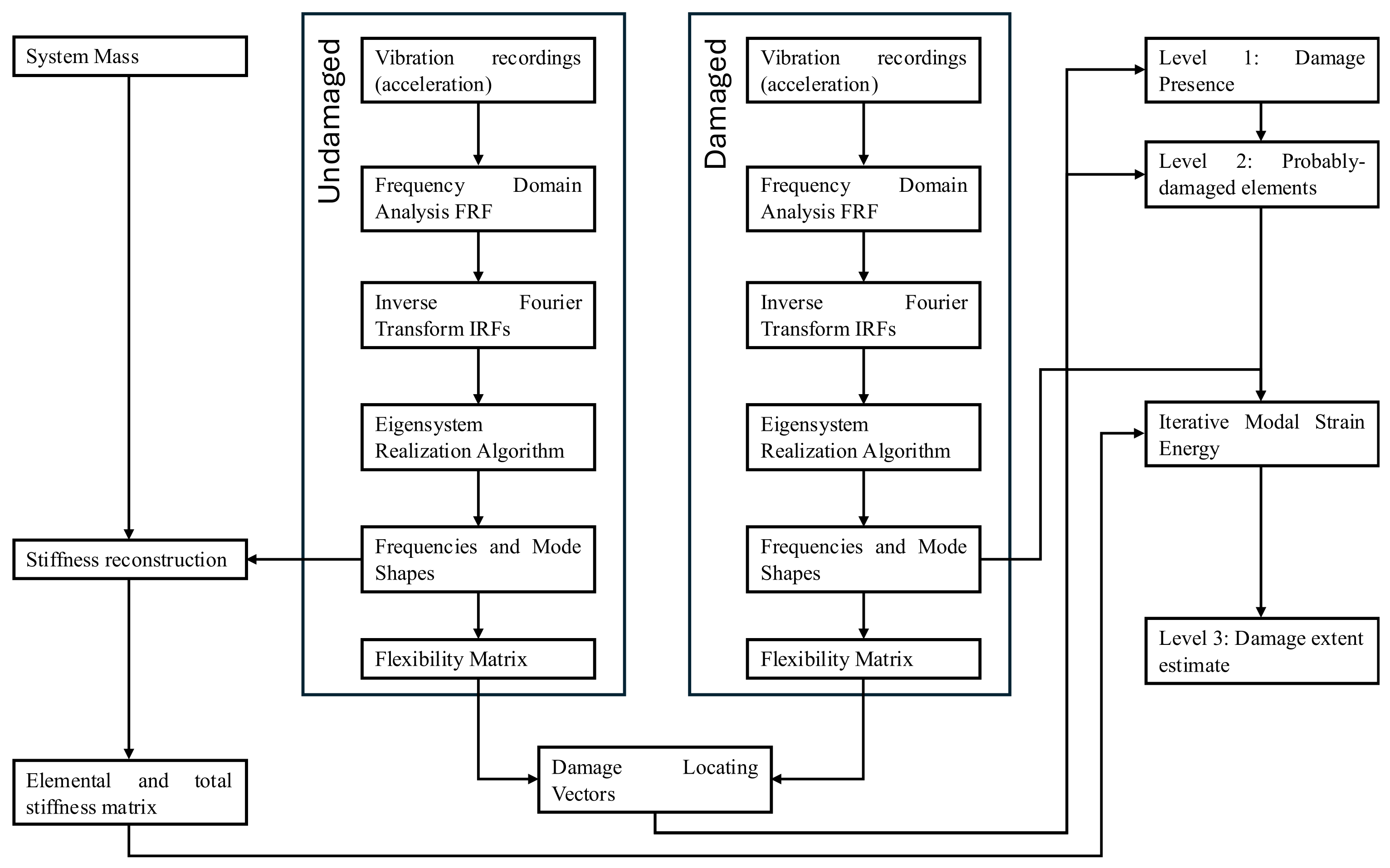
In Figure 1, the proposed Level 3 damage identification algorithm is summarized. Steps are as follows:

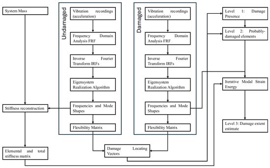
Figure 1. Damage identification algorithm flow chart.

• System identification frequencies and mode shapes of the undamaged and damaged structure are obtained by vibration recordings, frequency and time domain signal processing, and the use of the ERA.
• With the undamaged and damaged modal parameters, flexibility matrices are assembled, and the DLV technique is used for Level 1 and 2 damage identification.
• With the system masses and undamaged modal parameters, the total and elemental stiffness matrices are estimated.
• With the known undamaged stiffnesses, damaged modal parameters and the location of damage, an iterative strain energy procedure is used for calculating the damaged indices.

3. Dynamic Soil–Structure Interaction

The phenomena arising from the flexibility of the supporting soil are collectively known as soil–structure interaction (SSI). These effects are fundamentally categorized into static and dynamic conditions. Given the operational principles of VBSHM, this research focuses specifically on Dynamic Soil–Structure Interaction (DSSI), as it directly influences the modal parameters used for damage identification.

The most significant observable effects of DSSI include the modification of the system’s modal parameters, specifically its natural frequencies (or periods), mode shapes, and modal damping ratios [23,24]. Furthermore, modifications in the ground motion characteristics had been documented in the vicinity of the foundation, reflecting the filtered seismic demand reaching the superstructure.

Two primary analytical frameworks are available for DSSI: the direct method and the superposition (substructure) method. These can be further classified into analytical approaches, utilizing discrete springs and dashpots, and numerical methods. The direct method involves the simultaneous analysis of the soil–foundation–structure system under dynamic loading. This comprehensive approach is typically implemented via the Finite Element Method (FEM), allowing for the representation of complex foundation geometries and non-linear behavior.

On the other hand, superposition methods involve decomposing the complex DSSI problem into independent, sequential subsystems. Following the framework established by Kausel [25], the total dynamic response is treated as the linear combination of kinematic and inertial interactions.

Using the superposition method, DSSI is solved by:

▪

Kinematic Interaction: This represents the response of a massless foundation and superstructure to dynamic excitation. It focuses on determining the Effective Foundation Input Motion (EFIM) by accounting for wave diffraction caused by the foundation’s geometry and embedment depth. This is essentially a geometrical problem where the rigidity of the foundation “averages” the spatially varying ground motions. Kinematic interaction typically results in a reduction in high-frequency translational displacement while simultaneously inducing rocking and torsional components that were not present in the free-field motion.

▪

Inertial Interaction: This is defined by the response of the flexible-base system to the effective motion generated during the kinematic stage. In this phase, the analysis accounts for the inertial forces arising from the masses of both the foundation and the superstructure. The primary consequences of inertial interaction include a significant lengthening of the fundamental period (due to the added flexibility of the soil), an increase in the system’s damping ratio (resulting from radiation and hysteretic energy dissipation in the soil), and a potential modification of the inelastic structural response.

In this research, the superposition method was adopted due to its practical efficiency and clarity in isolating individual phenomena. Under this framework, DSSI effects were progressively integrated into the experimental computer simulations, allowing for a systematic evaluation of damage detection precision and efficiency at each stage. The flexibility effects considered include the site-effect, wave diffraction (kinematic interaction), and the modification of the system’s dynamic properties (inertial interaction).

To account for kinematic effects, an approximate solution following Kausel [25] was implemented, where the transfer functions for foundation translation $Q_h$ and rocking $Q_r$ for a shallow foundation are defined as follows:

$$Q_h\left(\omega \right)=\{\begin{array}{ll}\cos \left({\displaystyle \frac{\pi \omega }{2{\omega }_e}}\right)& \mathrm{if} \omega \le 0.70{\omega }_e\\ 0.453& \mathrm{if} \omega >0.70{\omega }_e\end{array}$$

(22)

$$Q_r\left(\omega \right)=\{\begin{array}{ll}0.257\left(1-\cos \left({\displaystyle \frac{\pi \omega }{2{\omega }_e}}\right)\right)& \mathrm{if} \omega \le {\omega }_e\\ 0.257& \mathrm{if} \omega >{\omega }_e\end{array}$$

(23)

where in Equations (22) and (23) ω_e is the depth fundamental frequency given by

$${\omega }_e={\displaystyle \frac{\pi V_s}{2D}}$$

(24)

In Equation (24), V_s is the soil deposit shear wave velocity (m/s) and D is the foundation depth (m).

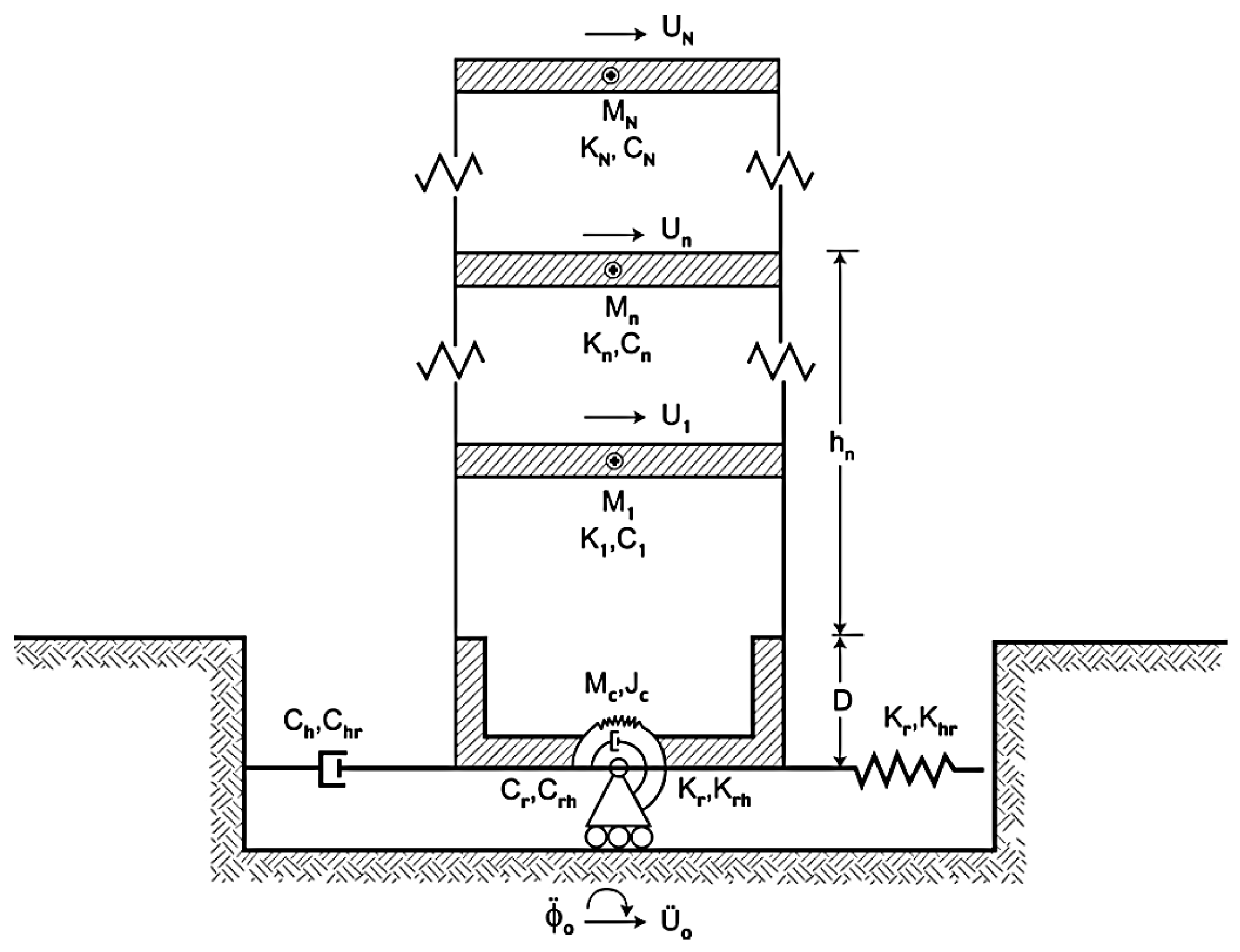
For inertial effects, a set of coupled multiple degrees of freedom formulation by Avilés [23] and Fernández and Avilés [24] was used (Figure 2)

$$\left[M_s\right]\left\{{\ddot{u}}_s\right\}+\left[C_s\right]\left\{{\dot{u}}_s\right\}+\left[K_s\right]\left\{u_s\right\}=-{\ddot{u}}_o\left\{M_o\right\}-{\ddot{\mathsf{\Phi }}}_o\left\{J_o\right\}$$

(25)

where in Equation (25) $\left\{u_s\right\}={\left\{\left\{u_e\right\} u_c {\mathsf{\Phi }}_c\right\}}^T$ is the system displacement vector, which contains the structure’s relative to base displacements $\left\{u_e\right\}$, the foundation translation $u_c$ and rocking ${\mathsf{\Phi }}_c$. On the other hand, $\left\{M_o\right\}$ and $\left\{J_o\right\}$ are load vectors for the effective translation ${\ddot{u}}_o$ and rocking ${\ddot{\mathsf{\Phi }}}_o$ (kinematic) respectively. Matrices $\left[M_s\right]$, $\left[C_s\right]$ and $\left[K_s\right]$ are the system mass, damping and stiffness matrices, given by

$$\left[M_s\right]=\left[\begin{array}{ccc}\left[M_e\right]& \left[M_e\right]\left\{I\right\}& \left[M_e\right]\left\{H\right\}\\ {\left\{I\right\}}^T\left[M_e\right]& {\left\{I\right\}}^T\left[M_e\right]\left\{I\right\}+M_c& {\left\{I\right\}}^T\left[M_e\right]\left\{H\right\}+M_{c}E\\ {\left\{H\right\}}^T\left[M_e\right]& {\left\{H\right\}}^T\left[M_e\right]\left\{I\right\}+M_{c}E& {\left\{H\right\}}^T\left[M_e\right]\left\{H\right\}+J_c\end{array}\right]$$

(26)

$$\left[C_s\right]=\left[\begin{array}{ccc}\left[C_e\right]& \left\{0\right\}& \left\{0\right\}\\ {\left\{0\right\}}^T& C_h& C_{hr}\\ {\left\{0\right\}}^T& C_{hr}& C_r\end{array}\right]$$

(27)

$$\left[K_s\right]=\left[\begin{array}{ccc}\left[K_e\right]& \left\{0\right\}& \left\{0\right\}\\ {\left\{0\right\}}^T& K_h& K_{hr}\\ {\left\{0\right\}}^T& K_{hr}& K_r\end{array}\right]$$

(28)

where $\left[M_e\right]$, $\left[C_e\right]$ and $\left[K_e\right]$ are the structure mass, damping and stiffness matrices. $M_c$, $J_c$ and $E$ are the foundations mass and rotational inertia, and the semi-depth respectively. The terms $C_m$ and $K_m$ where $m=h, hr$ or $r$ are the translation, coupled and rocking impedance functions. In this research, the impedance function form was used [26], where

$$K_m=K_m^o\left(k_m-2{\xi }_s{\eta }_m{c}_m\right)$$

(29)

$$\omega C_m=K_m^o\left({\eta }_m{c}_m+2{\xi }_s{k}_m\right)$$

(30)

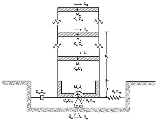
Figure 2. Multiple degree of freedom system with DSSI (after Fernández-Sola and Avilés [24]).

In which coefficients $K_m^o$, $k_m$, ${\eta }_m$ and $c_m$ are given from solutions by Gazetas [27], and Sieffert and Cevaer [28]. And the soil damping ratio ${\xi }_s$ was taken as 3%.

4. Simulation Scheme

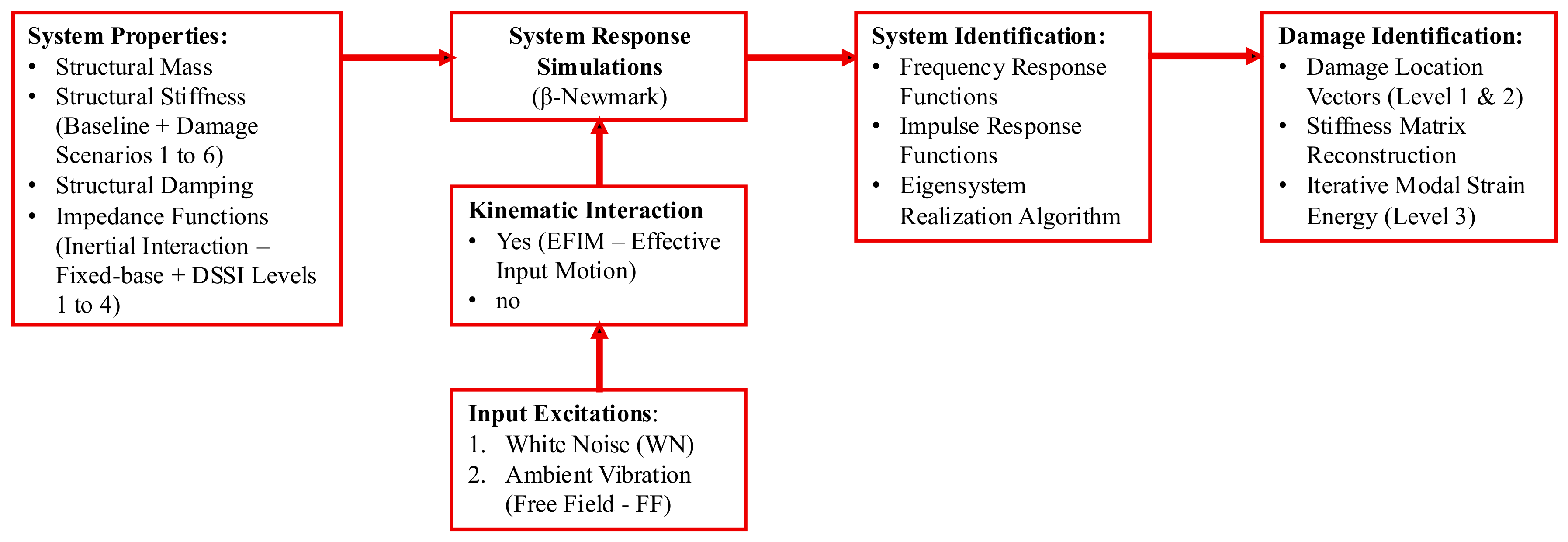
To evaluate the impact of DSSI on the performance of VBSHM algorithms, a comprehensive suite of computer simulations was conducted. These simulations were designed to progressively incorporate the superposition effects of the site’s excitation frequency content (site-effect), the filtering influence of foundation wave propagation (kinematic interaction), and the dynamic coupling of the flexible-base system (inertial interaction). This incremental approach allows for a precise quantification of how each DSSI component affects the reliability of damage detection and characterization (Figure 3).

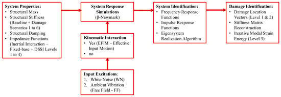
Figure 3. Simulation scheme flow chart.

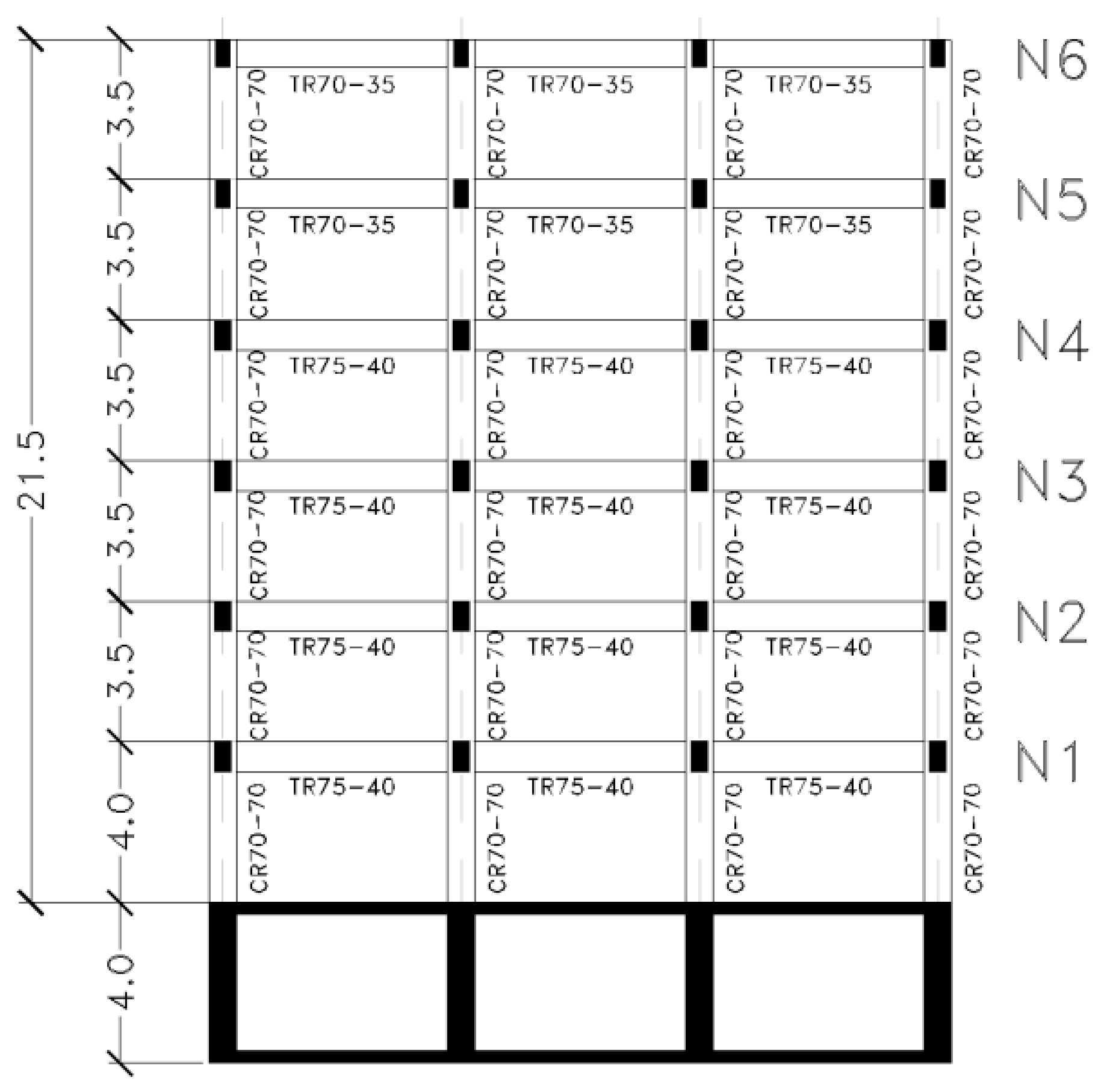
The DSSI evaluation was conducted using a simplified two-dimensional 6-DOF (degree-of-freedom) lumped-mass model, representing a hypothetical symmetrical reinforced concrete building. The structural configuration, as detailed in Figure 4, features 6 m spans, 70 cm square columns (CR70-70) and rectangular beams of two types: TR75-40 (40 cm × 75 cm) and TR70-35 (35 cm × 70 cm).

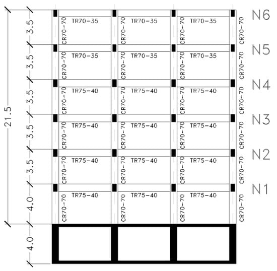
Figure 4. Reinforced concrete 6DOF system used for VBSHM under DSSI effects.

The structure was modeled as a lumped-mass moment-resisting frame (MRF). The Young’s Modulus (E) for the reinforced concrete was set at 25,685 MPa, with a corresponding volumetric weight of 2400 kg/m³. The mass distribution accounted for a 13 cm thick slab as the floor system, incorporating both dead loads (2.6 kN/m² for typical floors and 2.0 kN/m² for the roof) and live loads expected during transient events, taken according to their use category from the Mexico City Building Code [29] (1.8 kN/m² for typical floors and 0.7 kN/m² for the roof) as mass sources. No infills were considered in modeling; dead and live loads were developed assuming an office-type infrastructure. Based on these mechanical properties and loading conditions, the computed mass (m_i) and stiffness (k_i) components for each story are summarized in Table 1.

Table 1. 6 DOF system masses and stiffness components.

Story	Mass (kg)	Stiffness (kN/m)
1	39,810	12,019.47
2	39,450	17,941.59
3	39,450	17,941.59
4	39,450	17,941.59
5	37,750	17,941.59
6	29,620	17,941.59

To evaluate the influence of the input excitation’s frequency content under soft-soil conditions—which deviate significantly from the idealized characteristics of Gaussian white noise—actual ambient vibration data from the “Roma Norte” lakebed zone in Mexico City were utilized. According to the Mexico City Building Code [29], the recording site is characterized by a dominant site period of 2.1 s. Three 300 s orthogonal recordings, sampled at 256 Hz, were collected. The horizontal components (channels 2 and 3) were selected as representative of the site conditions and applied as the excitation source for both the baseline and damaged state simulations.

Standard digital signal processing (DSP) protocols were applied to the input signals, including baseline correction. Subsequently, a 12th-order bandpass Butterworth filter was implemented, with corner frequencies set between 0.20 Hz and 30 Hz. The output dynamic responses were subjected to the same processing criteria to maintain consistency across the input–output relationship required for system identification.

Kinematic effects were evaluated by modeling a rigid box foundation with a length of 18 m and an embedment depth of 4 m. The soft-soil deposit was assumed to have a total depth of 39.38 m. This stratigraphic configuration is physically consistent with the documented 2.1 s site period, as it corresponds to a shear wave velocity (V_s) of 75 m/s. This low velocity is characteristic of the highly compressible clay deposits found in the Mexico City lakebed zone, providing a realistic scenario for investigating wave diffraction and signal filtering at the foundation level.

To evaluate a broad spectrum of interaction levels, four distinct soil stiffness scenarios were modeled by incrementally adjusting the shear wave velocity (V_s). Table 2 summarizes the stratigraphic properties for each case, including the soil deposit depth (H_s) and the fundamental site period (T_s). The relative intensity of the interaction is quantified by a dimensionless DSSI parameter (H_eT_s/H_sT_e), which relates the structural and soil stiffness through the ratio. This parameter serves as an indicator of the expected influence of soil flexibility on the dynamic response, where higher values denote a more pronounced coupling between the system and the foundation.

Table 2. Shear wave velocity, soil deposit depth, site period and H_eT_s/H_sT_e ratio for 4 DSSI intensity levels.

DSSI Level	1	2	3	4
Vs (m/s)	250	150	100	75
Hs (m)	39.4	39.4	39.4	39.4
Ts (s)	0.63	1.05	1.58	2.1
HeTs/HsTe	0.60	1.00	1.50	2.00

Different damage scenarios were explored with damage located in the first and second stories in combination of 10%, 20% and 40% reduction in the lateral stiffness taken as structural damage (Table 3). Damage locations in the simulation scheme were not rigorously defined; they were selected based on the common assumption that interstory drift demands in shear buildings tend to be larger within the first third of the building height. Also, a test run with zero damage was taken to explore false positives with the VBSHM algorithm.

Table 3. Simulations of damage scenarios for DSSI effects exploration.

Scenario	1	2	3	4	5	6
Lateral Stiffness reduction (%)	10	20	40	10	20	40
Damage Location (story)	1	1	1	2	2	2

Dynamic simulations were executed using a step-by-step integration in the time domain, employing Newmark’s linear acceleration β-method [30]. To account for the frequency-dependent nature of the impedance functions, an iterative computational approach was implemented. The procedure initially assumed the fixed-base natural frequencies to determine the soil–foundation dynamic stiffness and damping. Subsequently, the foundation–structure mass and stiffness matrices were assembled, and the eigenvalue problem was solved repeatedly to update the system’s frequencies until numerical convergence was achieved.

Beyond the combinations of damage scenarios and soil flexibility, the simulations were conducted by progressively incorporating additional physical variables. This incremental approach was designed to evaluate the VBSHM algorithm’s performance at distinct levels of complexity:

• Site-Effect Only: Analysis using raw vibration recordings obtained under soft-soil conditions as the input, bypassing foundation filtering.
• Site + Kinematic Effects: Integration of the Effective Foundation Input Motion (EFIM), where the site recordings are modified by the transfer functions that represent the soil–foundation geometry.
• Site + Kinematic + Inertial Effects: The complete DSSI model, considering both the effective excitation and the dynamic response of the superstructure coupled with a flexible base.

The VBSHM algorithm performance was evaluated in terms of the number of positive or negative falsely damaged elements identified, the weighted stress index WSI, the number of iterations needed for the IMSE damage intensity estimation, and the actual value of identified versus simulated stiffness reduction. Results were plotted for each damage and DSSI scenario.

For Frequency Response Functions (FRF) calculations, the Welch method was used for spectral estimation, with 2048 Fast Fourier Transform (FFT) points, and 50% overlap using Hanning windows. For ERA identification purposes, a total of 210 data rows and 70 data columns were used for the Hankel matrices assembly. On the DLVs, stiffness reconstruction and IMSE only information on the first (fundamental) mode was used.

5. Results

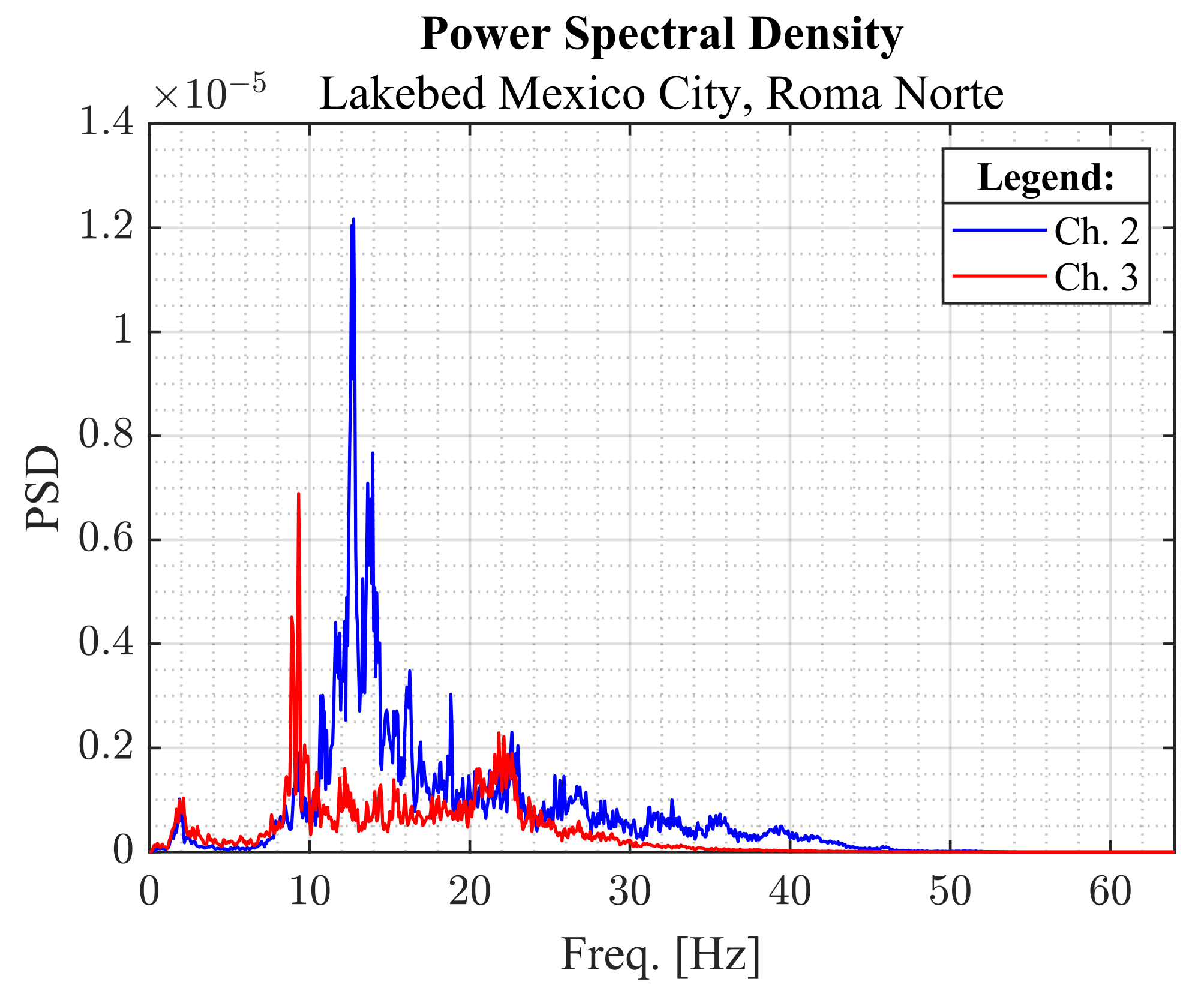
The frequency content of the free-field ambient vibration recordings for soft-soil conditions was analyzed, with results presented in Figure 5. The power spectral density (PSD) indicates that the energy is not uniformly distributed across the frequency spectrum, clearly deviating from the idealized white-noise assumption. While a broad range of frequencies is present, significant differences are observed between the horizontal components; however, they exhibit strong similarities in the low-frequency range (below 10 Hz). These characteristics confirm that two distinct, yet site-consistent, time histories arise from the recorded motions, thereby providing a robust baseline for evaluating the algorithm under realistic seismic conditions.

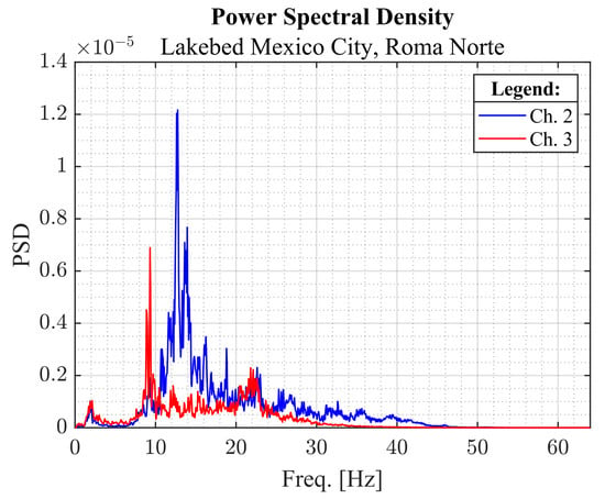
Figure 5. Power spectral densities for channels 2 and 3 of site recordings on the lakebed, Mexico City, Roma Norte.

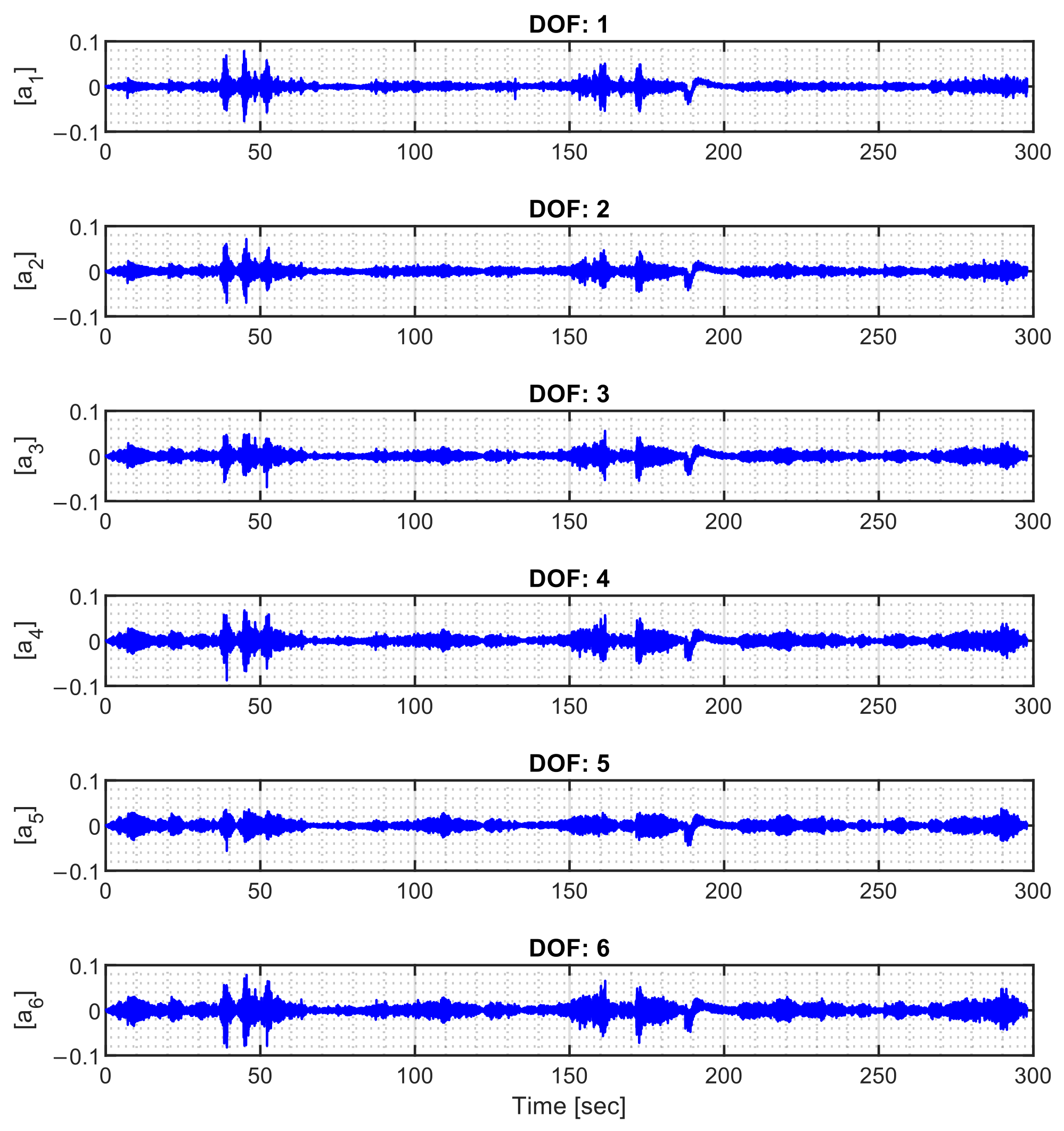
The fixed-base output responses (absolute acceleration, units cm/s²) of the undamaged system subjected to the channel 2 (Ch. 2) recording are presented in Figure 6. This represents the structural response under an input excitation whose frequency content corresponds to soft-soil conditions. Subsequently, the simulation was repeated for damage scenario 5 (as detailed in Table 3) using the channel 3 (Ch. 3) input. System identification techniques were applied to these fixed-base scenarios and compared against a white-noise benchmark. The results, summarized in Table 4 and Table 5, show the identified frequencies and damping ratios for the first three vibration modes. A high degree of consistency was observed, with numerical differences below 3% between the different excitation types.

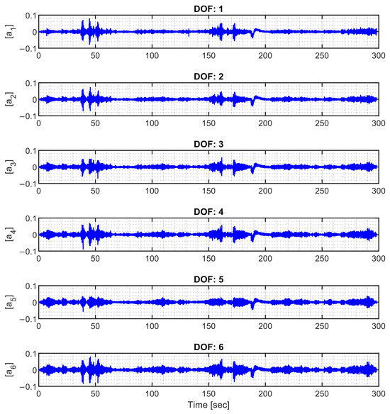
Figure 6. Fixed base, undamaged scenario time history responses for the 6DOF reinforced concrete building.

Table 4. Identified frequencies for baseline and damaged scenario 5, for white-noise (WN) test run versus free-field (FF) simulations.

Mode	Baseline		Damaged
	WN (Hz)	FF (Hz)	WN (Hz)	FF (Hz)
1	2.49	2.49	2.42	2.42
2	7.38	7.37	7.36	7.36
3	11.93	11.93	11.78	11.78

Table 5. Identified damping ratios for baseline and damaged scenario 5, for white-noise (WN) test run versus free-field (FF) simulations.

Mode	Baseline		Damaged
	WN (%)	FF (%)	WN (%)	FF (%)
1	1.39	1.36	1.33	1.30
2	2.69	2.69	2.72	2.73
3	4.18	4.14	4.21	4.20

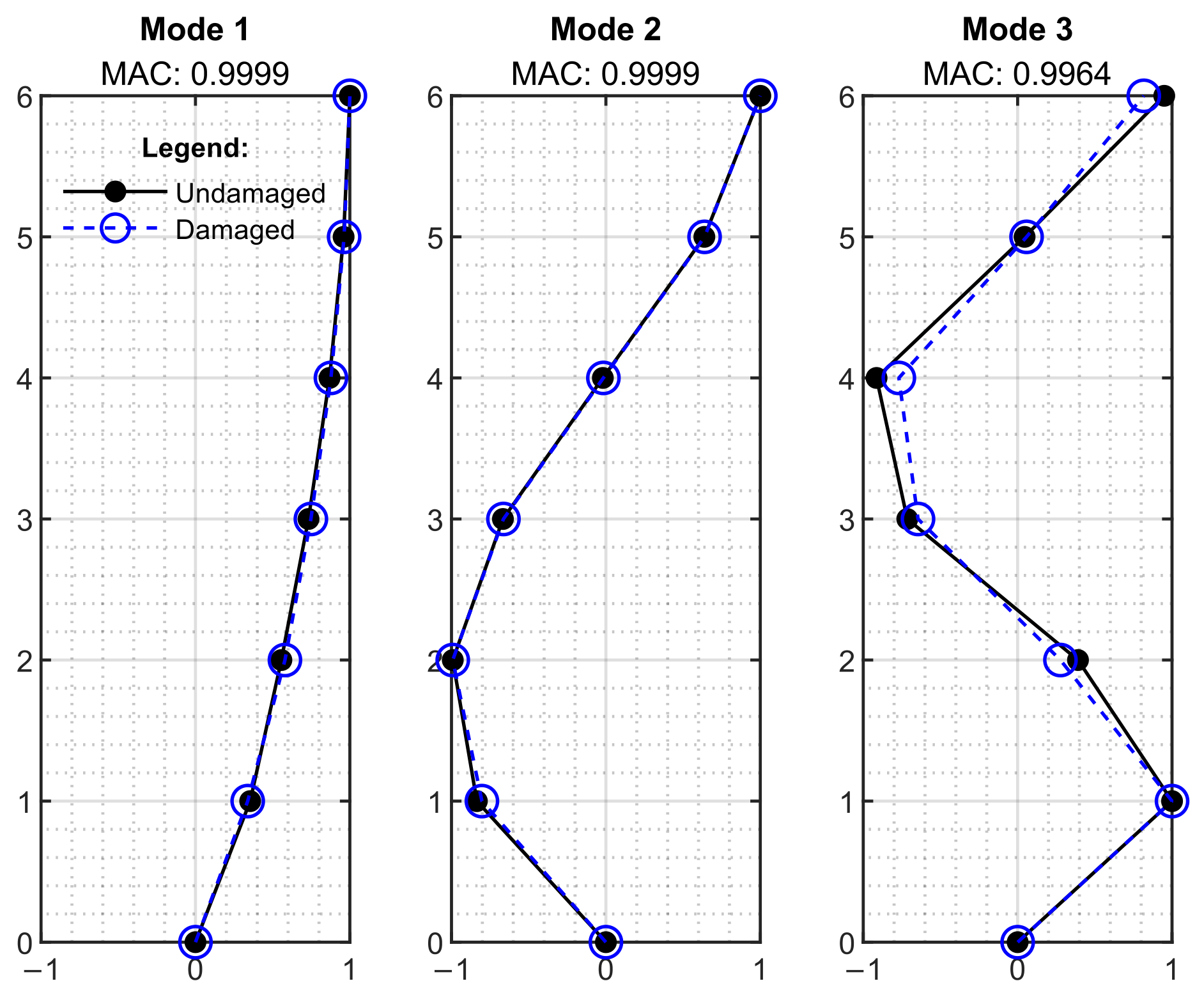
A comparison of the first three identified mode shapes for the baseline (undamaged) and damage scenario 5 is illustrated in Figure 7. The results indicate that the modal profiles remain remarkably similar despite the structural degradation. Quantitatively, the Modal Assurance Criterion (MAC) values were consistently above 0.99 for all compared modes. This high correlation underscores the low sensitivity of the MAC index for direct damage detection, as it fails to capture the localized stiffness changes that do not significantly alter the global eigenvector orientation.

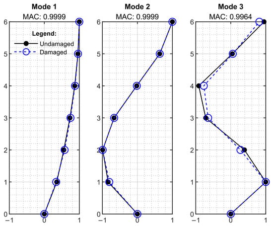
Figure 7. First 3 identified mode shapes in the baseline and damage scenario 5 under site effects.

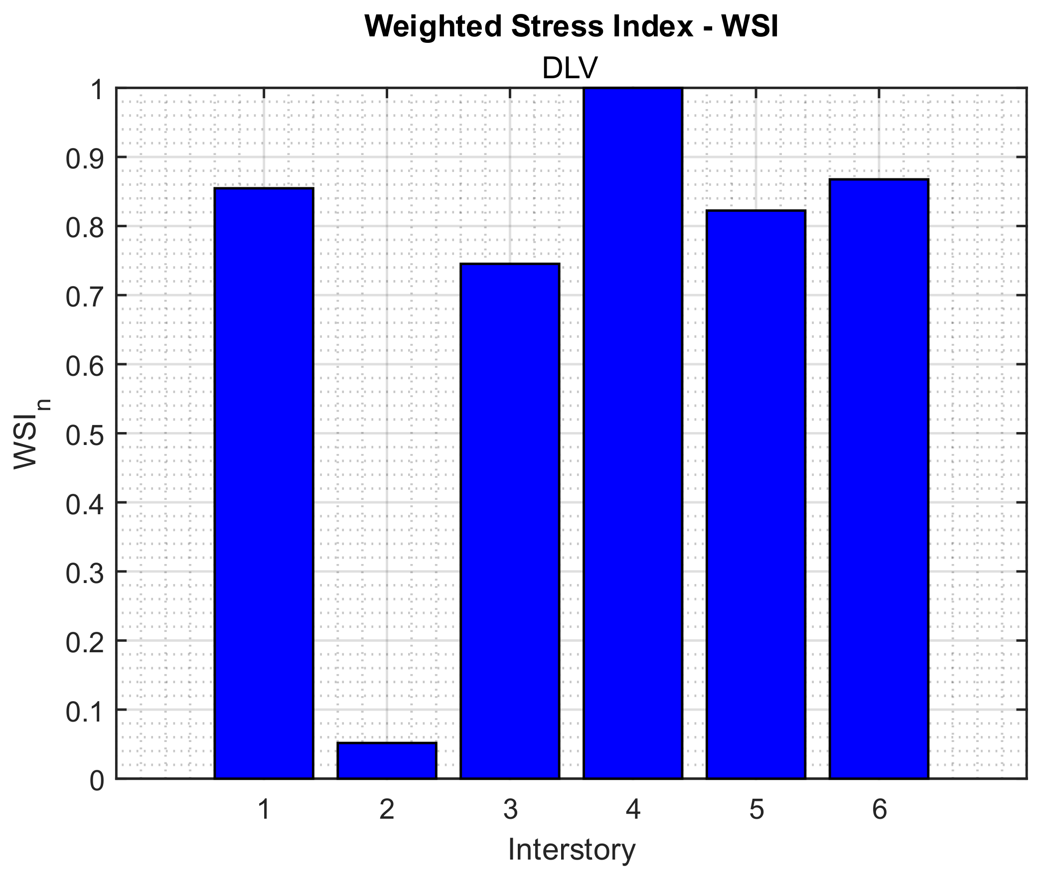
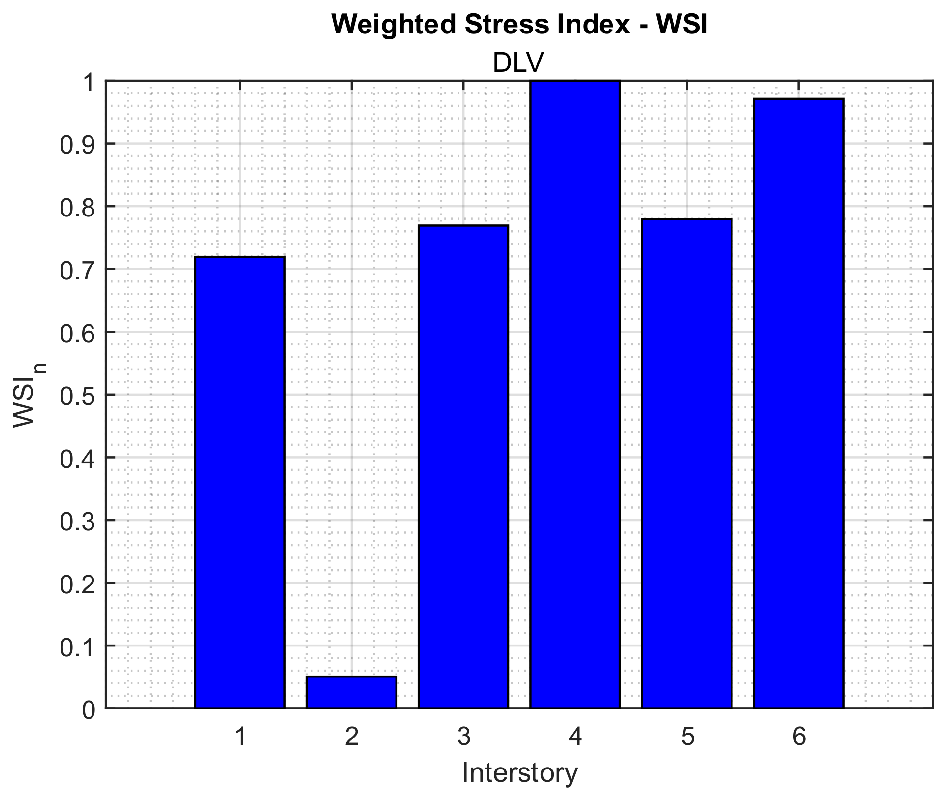
The weighted stress index for the damage scenario 5 is shown in Figure 8. A clear reduction in the second interstory DLV weighted stress index can be identified. Under this result, it can be said that a Level 1 damage identification has been achieved (there is the presence of DLVs). Also, Level 2 damage identification has been achieved, that is, damage has been predicted to be at the 2nd interstory, whose stress index is below the established threshold.

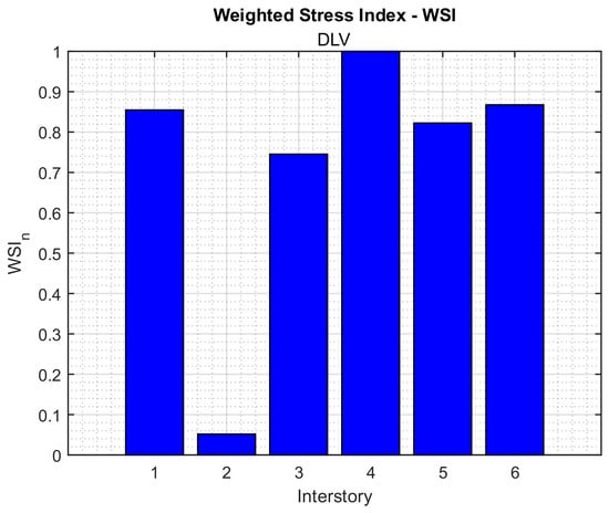
Figure 8. DLV weighted stress index under site effects.

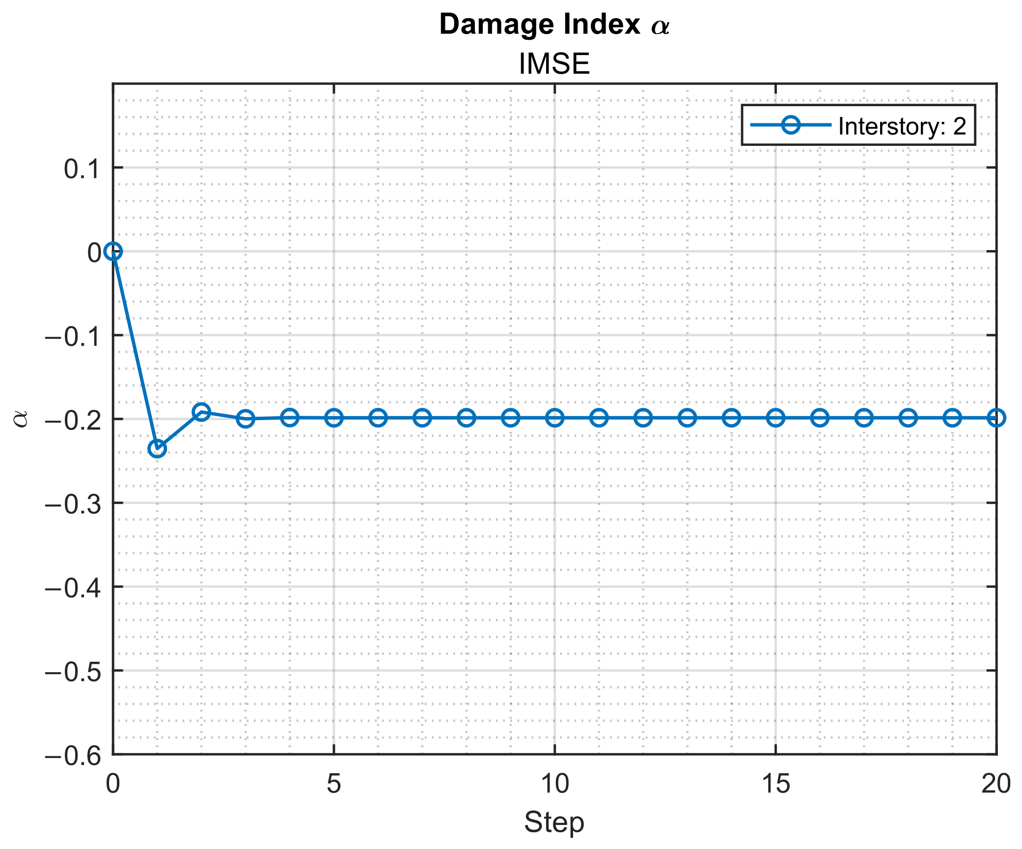
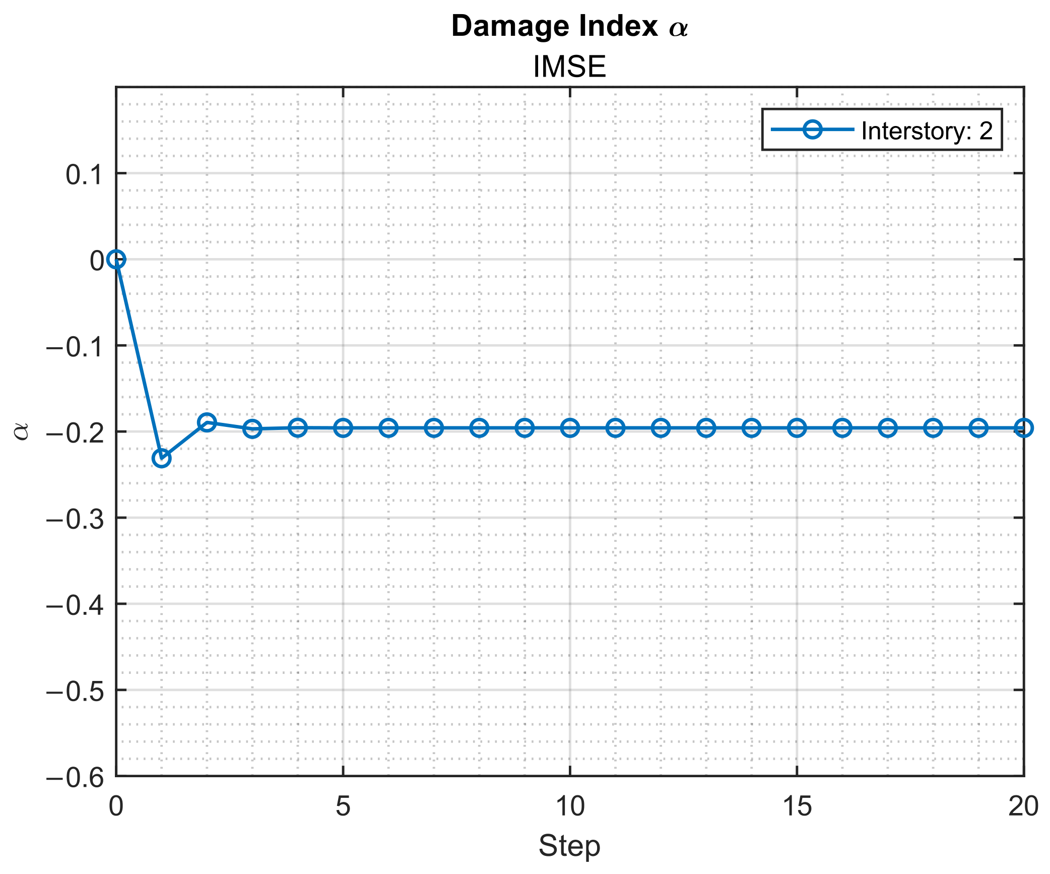
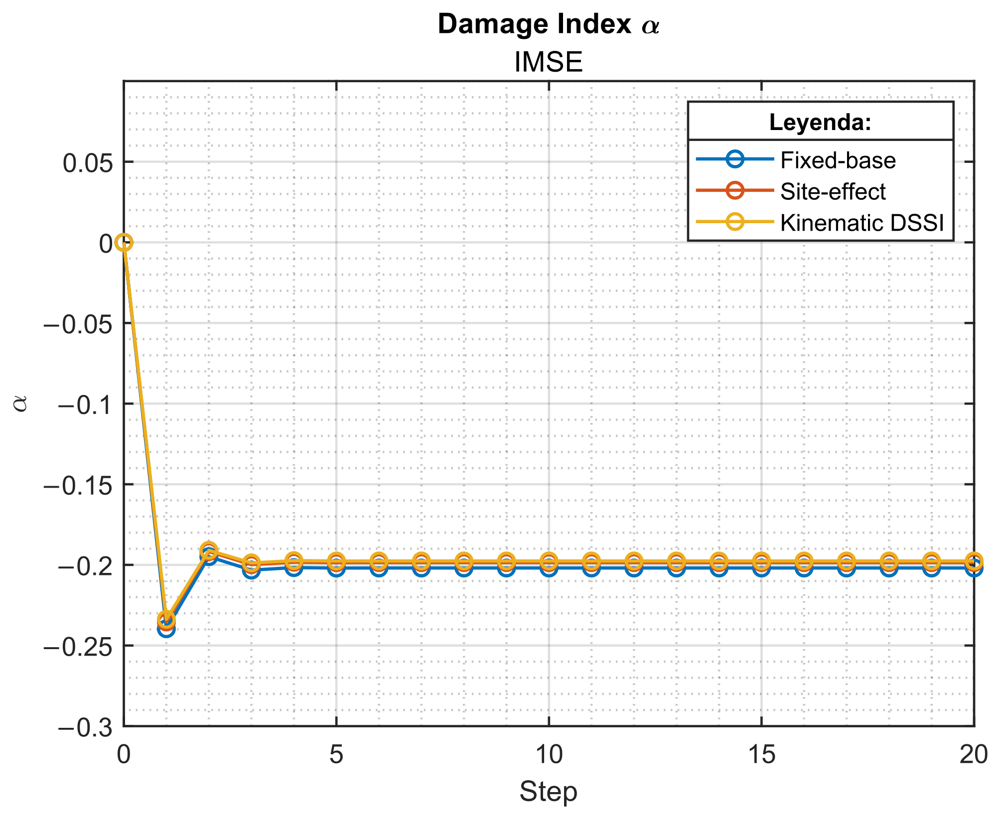
Under the assumption of localized damage in the 2nd interstory, the IMSE damage index estimation was performed, as illustrated in Figure 9. The convergence plots demonstrate high computational efficiency; in fewer than three iteration steps, the damage index stabilizes at −20%. This indicates that the VBSHM algorithm accurately captured the extent of the damage, correctly identifying a 20% reduction in lateral stiffness. Consequently, Level 3 damage identification (quantification) was successfully achieved, marking the successful completion of the algorithmic routine for the fixed-base scenario.

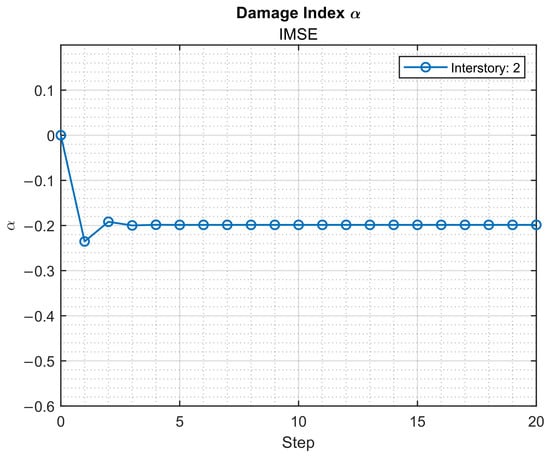
Figure 9. Damage index estimate IMSE iteration steps under site effects.

The subsequent simulation phase incorporated both site and kinematic effects, while maintaining a fixed-base condition. This scenario accounts for the frequency-dependent modification of the seismic input due to wave interference and diffraction caused by the foundation’s presence—a phenomenon referred to as the Effective Foundation Input Motion (EFIM). The resulting dynamic properties were compared against the white-noise (WN) benchmark, with identified natural frequencies and damping ratios summarized in Table 6 and Table 7, respectively.

Table 6. Baseline and damage scenario 5 identified mode frequencies comparison to effective input.

Mode	Baseline		Damaged
	WN (%)	EFIM (%)	WN (%)	EFIM (%)
1	2.49	2.49	2.42	2.42
2	7.38	7.37	7.36	7.36
3	11.93	11.93	11.78	11.78

Table 7. Baseline and damage scenario 5 identified damping ratios comparison to effective input.

Mode	Baseline		Damaged
	WN (%)	EFIM (%)	WN (%)	EFIM (%)
1	1.39	1.30	1.33	1.33
2	2.69	2.69	2.72	2.72
3	4.81	4.15	4.21	4.21

Following the identification of the modal properties under the EFIM, the VBSHM algorithm was deployed to assess damage localization and quantification. The WSI was computed to evaluate the spatial distribution of the identified changes (Figure 10), and the results of IMSE are shown in Figure 11. Despite the kinematic filtering of the input signal, the algorithm maintained high stability, demonstrating that the structural health assessment remains reliable even when the excitation energy is geometrically attenuated by the foundation.

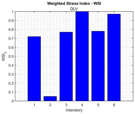
Figure 10. DLV weighted stress index under effective input.

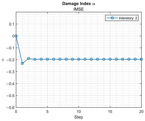
Figure 11. Damage index estimate IMSE iteration steps under effective input.

As observed in Figure 10, and consistent with the results in Figure 8, a large reduction in the WSI is clear at the second structural level. This localized drop confirms that an accurate Level 1 and 2 damage identification (detection and localization) is achieved even under the frequency-modified EFIM conditions. Furthermore, the convergence results in Figure 10 demonstrate that the IMSE damage index correctly identifies the −20% lateral stiffness reduction. This high level of precision validates the algorithm’s robustness against the geometric filtering effects inherent in kinematic interaction.

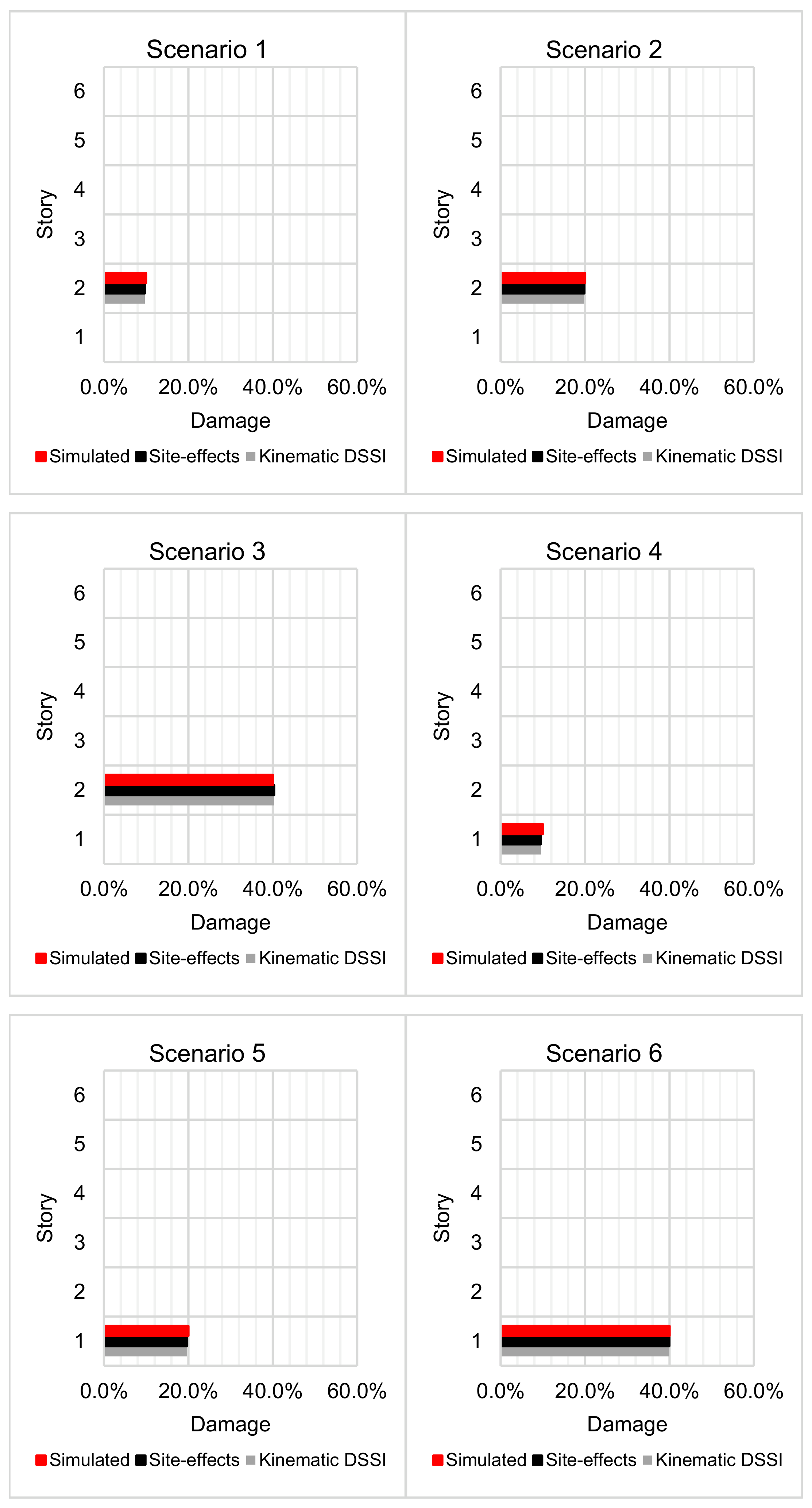
In Figure 12, a comprehensive summary of the results for the full spectrum of damage configurations detailed in Table 3 is shown, encompassing scenarios under white-noise excitation, free-field site effects, and kinematic interaction. The data demonstrate that the VBSHM algorithm achieved 100% reliability across all six damage scenarios, with zero false positives or false negatives reported. Furthermore, the damage indices were precisely estimated in both location and magnitude.

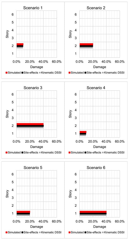
Figure 12. Damage identification summary of six scenarios under site effects and site + kinematic DSSI.

Following the exploration of site and kinematic effects, the final simulation phase incorporated site, kinematic, and inertial effects simultaneously. This comprehensive model accounts for the complex interplay between the soft-soil frequency content, the geometric filtering of the foundation, and the dynamic response of the superstructure on a flexible base. Unlike previous stages, this scenario introduces energy radiation and base motions (translation and rocking), which alter the system’s modal properties. This setup represents the most realistic and challenging condition for the VBSHM algorithm, as the inertial interaction can potentially mask structural damage by shifting the system’s natural frequencies and damping ratios.

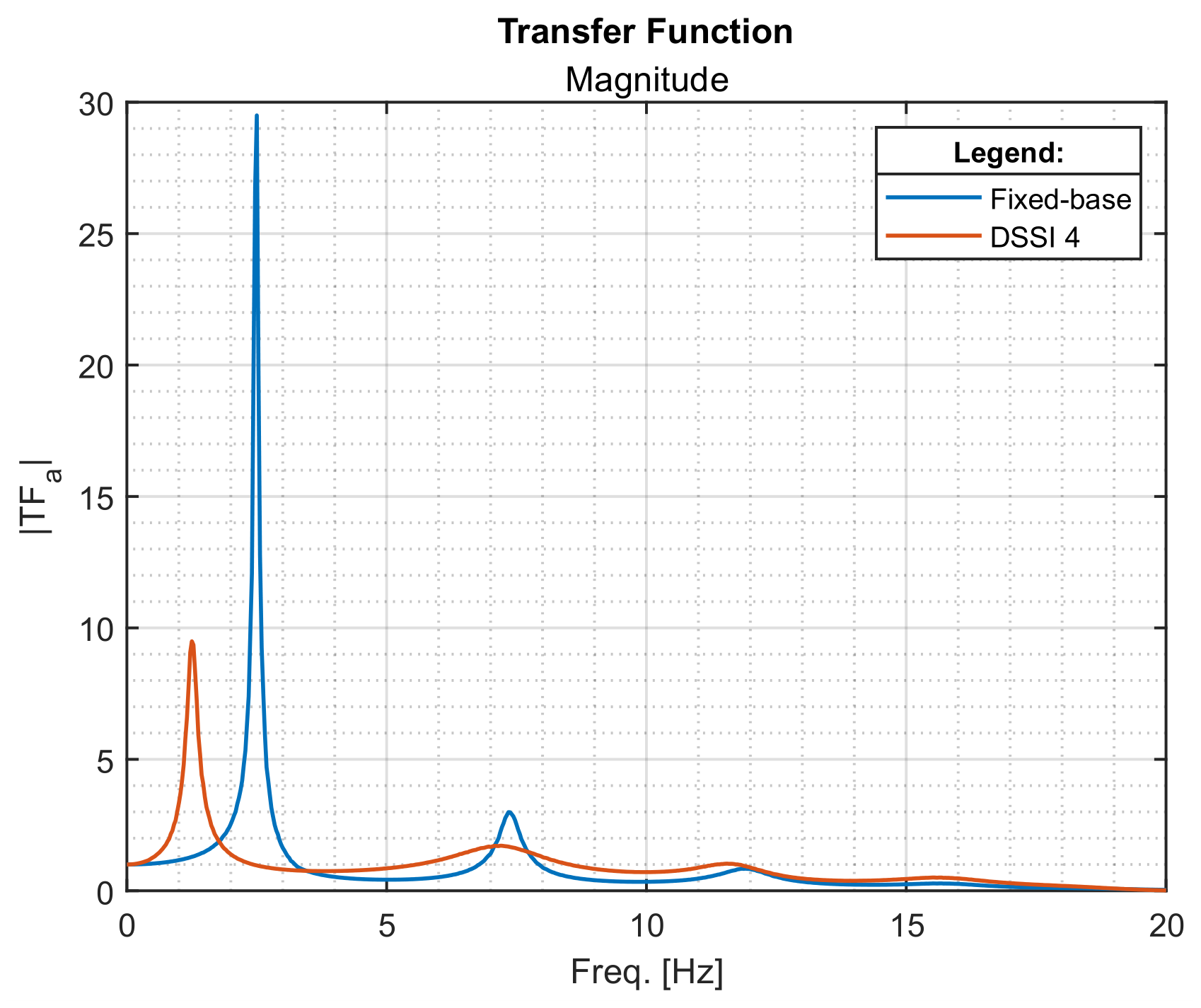
Acceleration transfer functions (TF_a) were computed to compare the fixed-base response against the most flexible soil condition (V_s = 75 m/s, DSSI Level 4), as shown in Figure 13. The spectral analysis reveals a significant leftward shift in the fundamental peak, confirming the lengthening of the system’s natural period due to base flexibility. Furthermore, the peak in the DSSI scenario exhibits a lower magnitude and a broader bandwidth, which is a direct consequence of the augmented damping (incorporating both material and radiation damping). Notably, the second and third modal peaks are heavily attenuated, indicating that the fundamental mode becomes increasingly dominant under SSI conditions compared to the fixed-base benchmark.

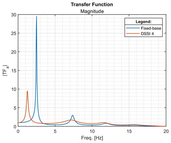
Figure 13. Fixed base and flexible base with DSSI 4 (V_s = 75 m/s) scenario transfer functions.

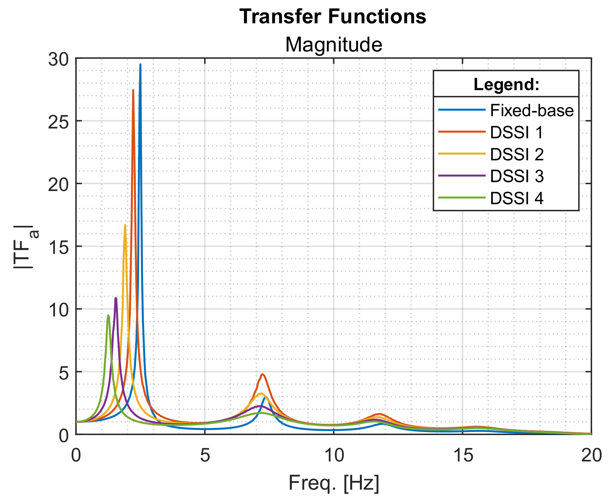
Figure 14 illustrates the comprehensive evolution of the acceleration transfer functions across the full range of shear wave velocities (V_s) detailed in Table 3. The plot captures the global dynamic response of the system as it transitions from a stiff to an increasingly flexible soil. It is evident that as V_s decreases, there is a discrete and systematic progression characterized by a significant lengthening of the fundamental period and a substantial increase in the system’s equivalent damping.

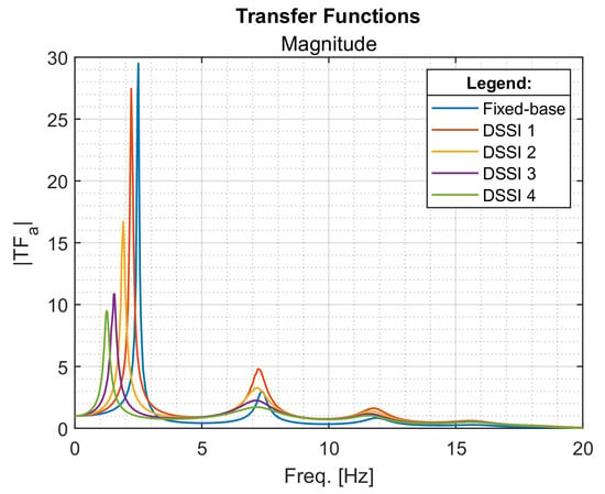
Figure 14. Fixed base and four DSSI flexible base intensity scenario transfer functions.

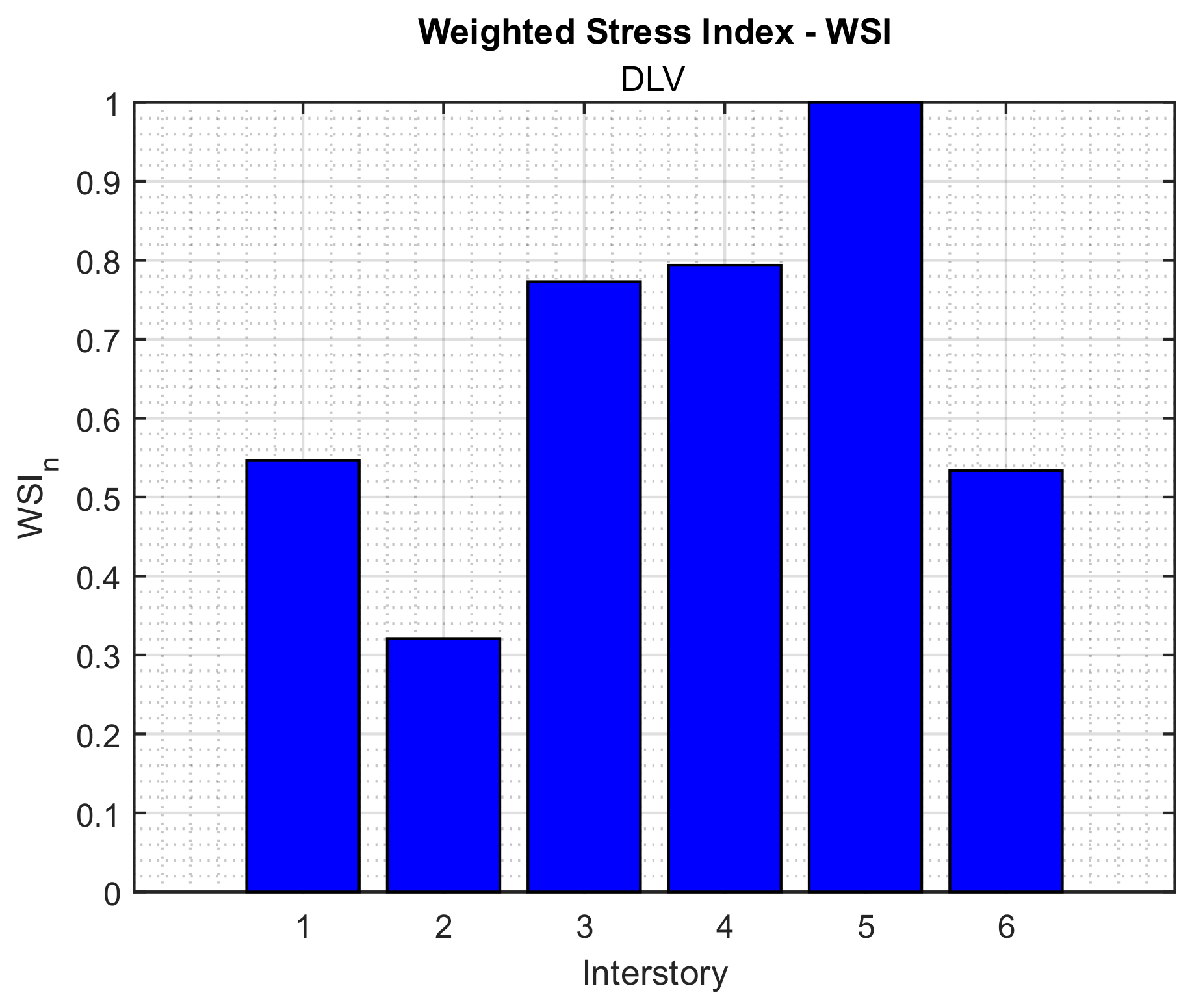
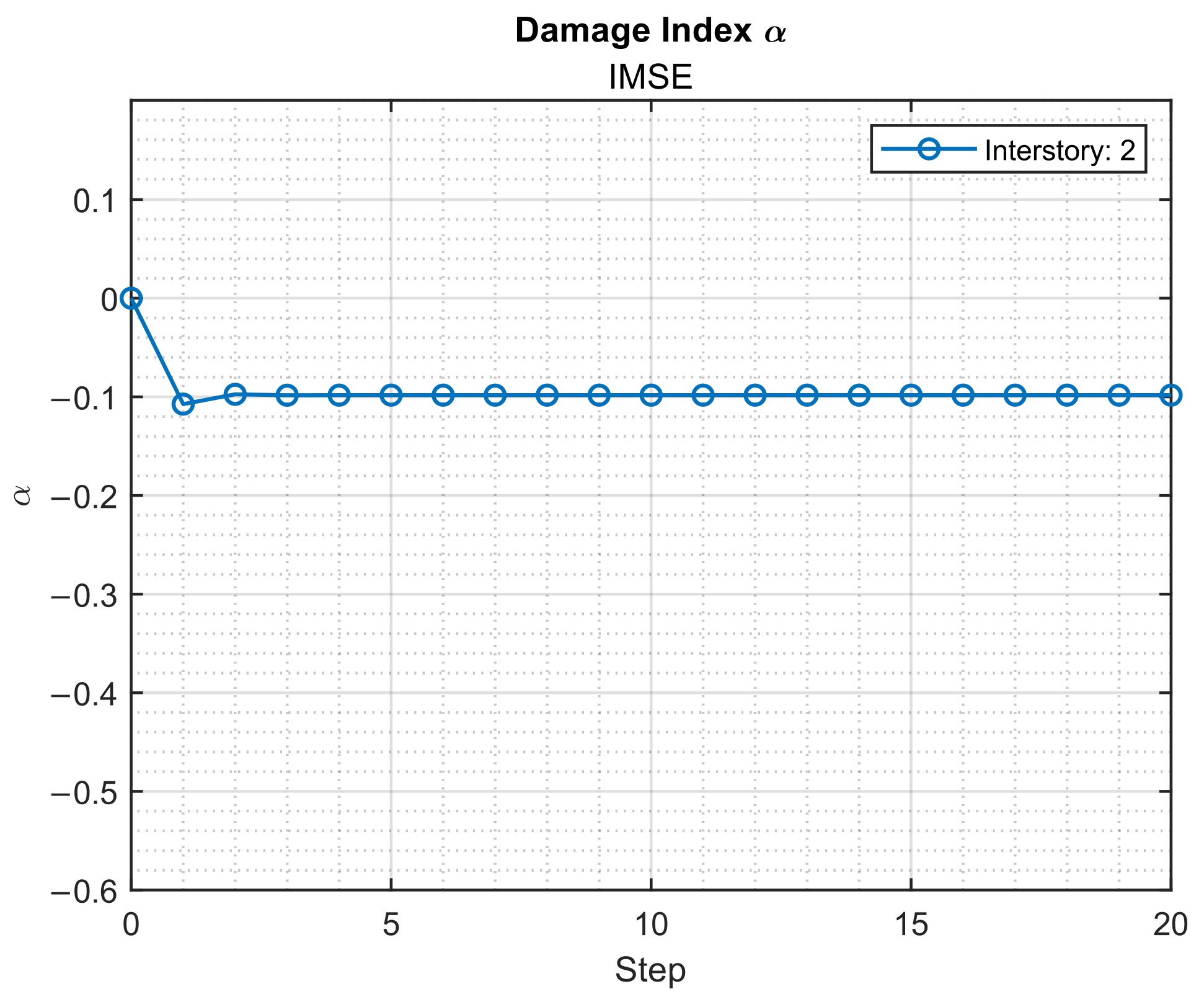
The performance of the algorithm under the most demanding conditions—damage scenario 5 coupled with the full range of soil flexibilities—is presented in Figure 15 (weighted stress index) and Figure 16 (IMSE damage index iterations).

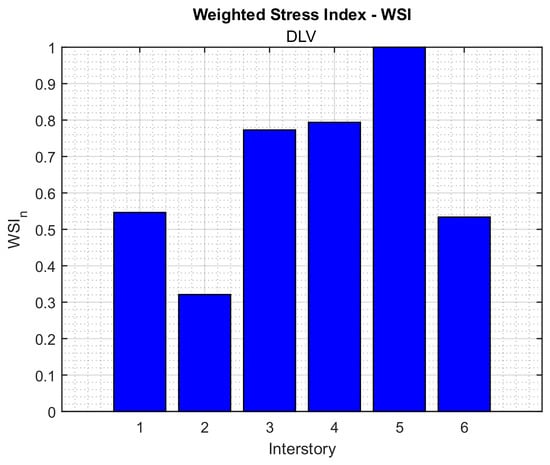
Figure 15. DLV weighted stress index under DSSI 4, damage scenario 5.

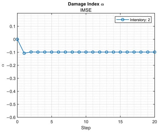
Figure 16. Damage index estimate IMSE iteration steps under DSSI 4, damage scenario 5.

In contrast to the results in Figure 11, the data in Figure 15 reveal a significant challenge in discriminating the damage signature. Both interstories 1 and 2 exhibit WSI near 40%, with the damaged interstory barely exceeding the 0.35 detection threshold, making it more difficult to select the probably damaged element.

Conversely, results from Figure 16 reveal that the damage quantification process was significantly compromised by the inertial effects. The algorithm estimated a 10% reduction in lateral stiffness, failing to capture the full extent of the 20% actual simulated degradation. This 50% underestimation indicates that DSSI effectively “masks” structural damage, as the system’s global flexibility becomes dominated by the soil–foundation interaction rather than the local stiffness loss.

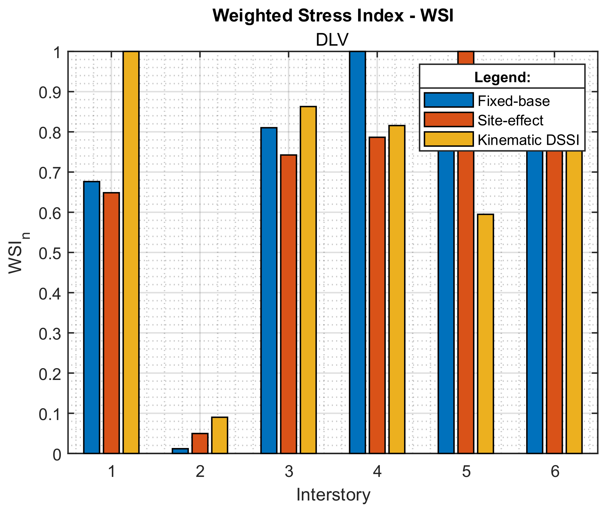
Figure 17 presents a comparative analysis of the WSI across three distinct simulation environments: fixed-base white noise, site-effect effective inputs, and the full DSSI integration (including kinematic interaction). The results demonstrate that both site effects and kinematic interaction exert a negligible influence on the WSI, preserving the algorithm’s localization accuracy. In these scenarios, the primary damage indicator consistently remains at the 2nd interstory.

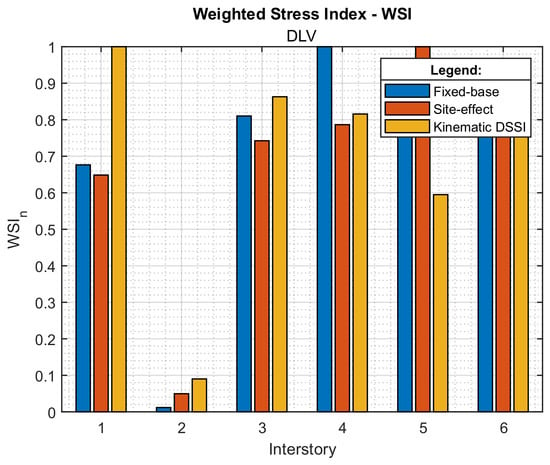
Figure 17. Fixed base, site-effect and site + kinematic DSSI, weighted stress index comparison.

The IMSE iteration results for fixed-base white noise, free-field site effects, and kinematic interaction are consolidated in Figure 18. Consistent with previous identification stages, the frequency content of the input signals—even those derived from soft-soil recordings—has a negligible impact on the algorithm’s performance, which consistently identifies a damage magnitude close to the simulated −20%.

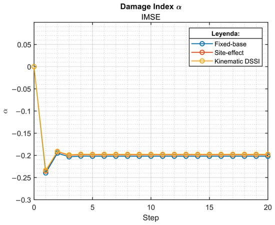
Figure 18. Fixed base, site-effect and site + kinematic DSSI, IMSE damage index comparison.

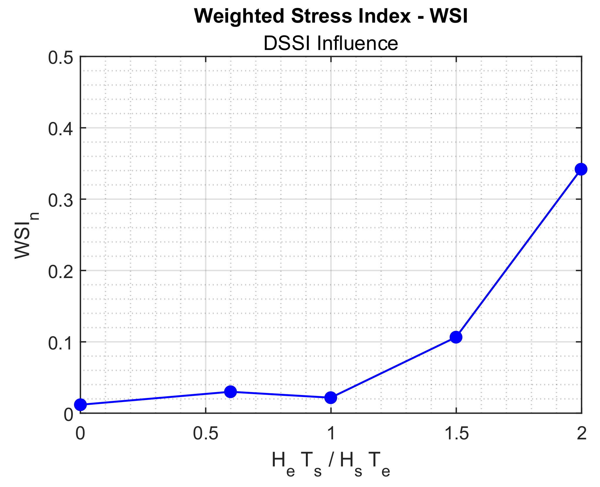
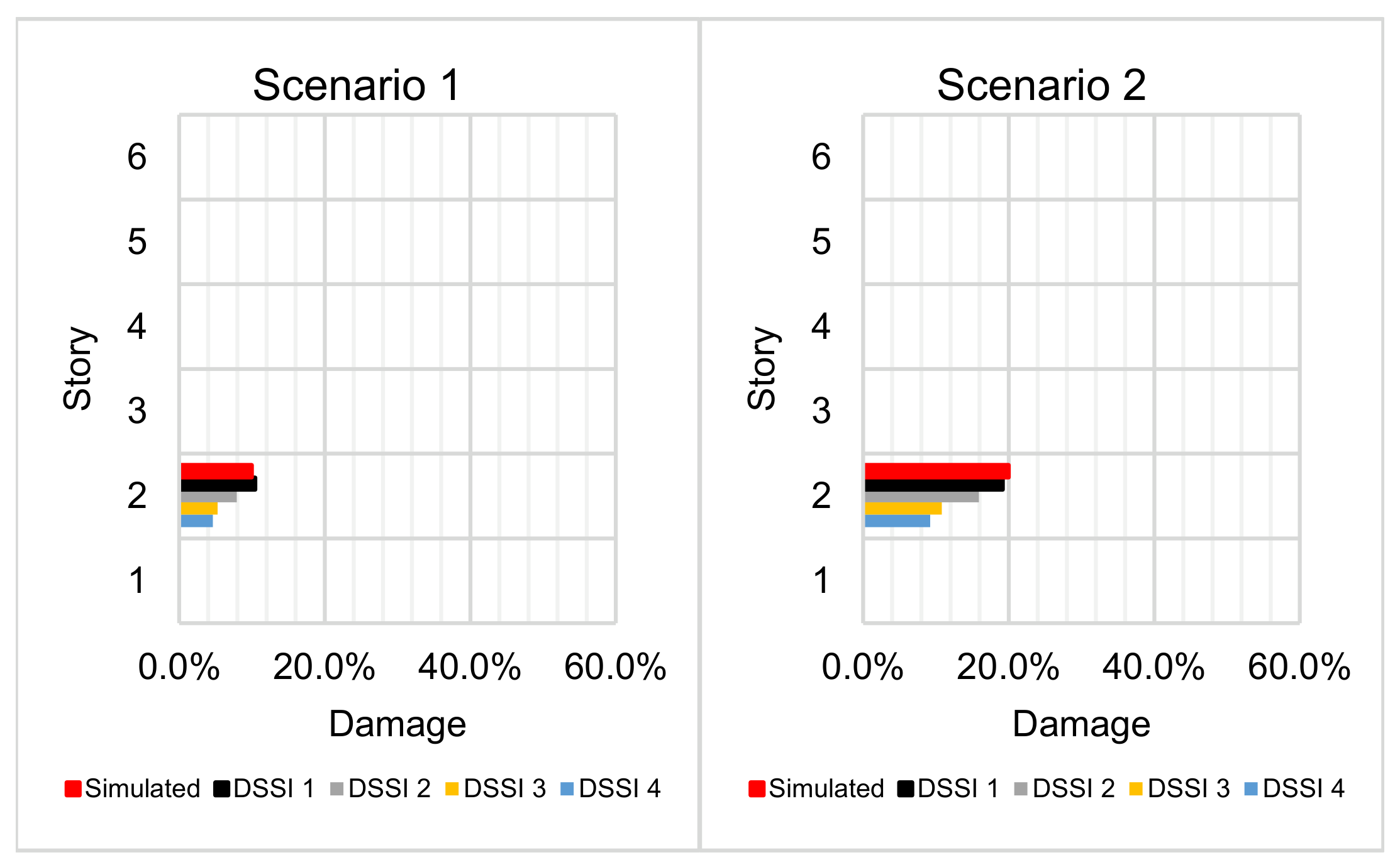
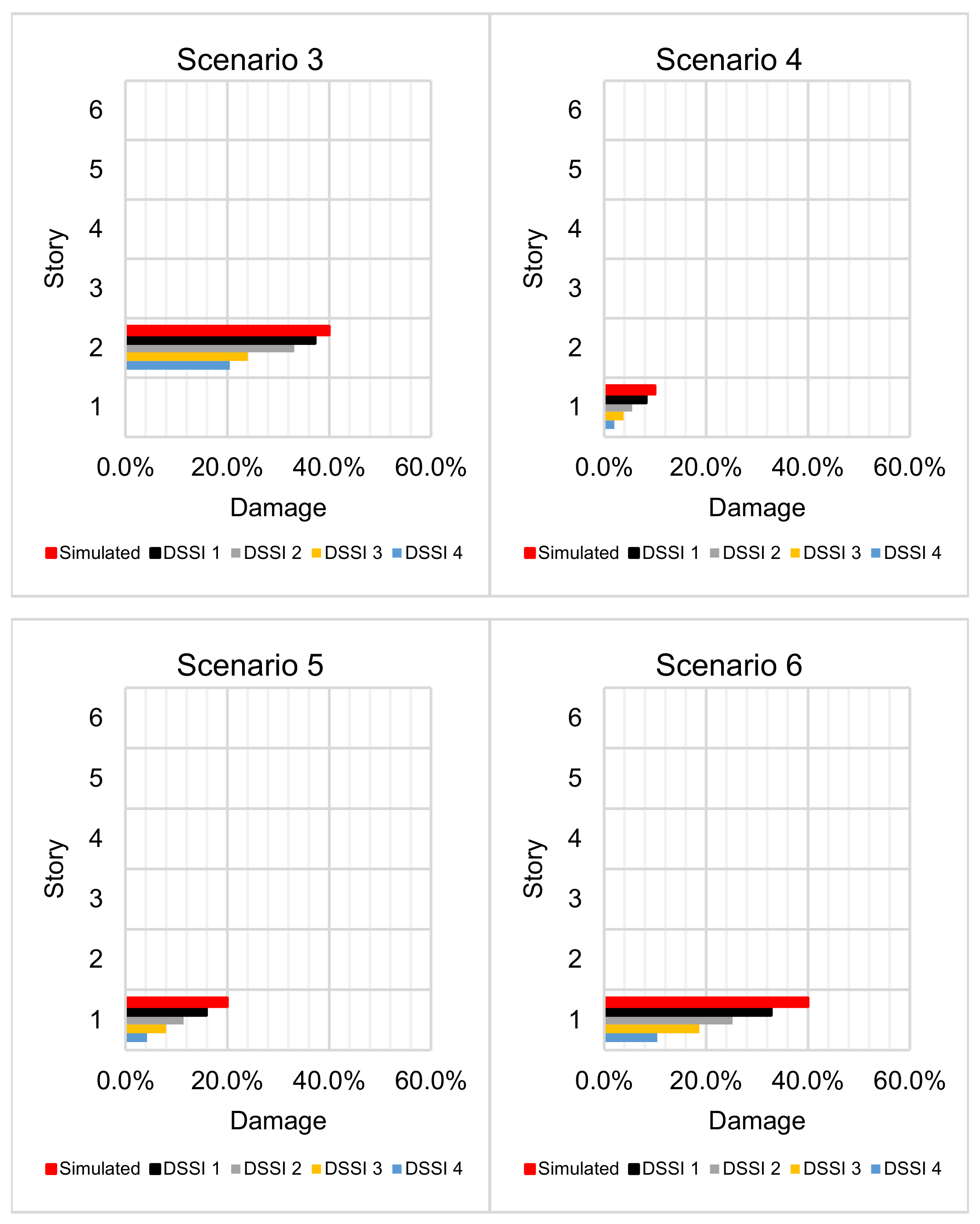
The evolution of the damaged-element weighted stress index as a function of the dimensionless structure-to-soil stiffness ratio is shown in Figure 19. A comparison between the soil flexibilities listed in Table 2 and the simulated damage is presented in Figure 20. As the soil becomes softer, the algorithm exhibits a progressive loss of accuracy. Nevertheless, in all scenarios, the presence and location of damage (Levels 1 and 2) are successfully identified.

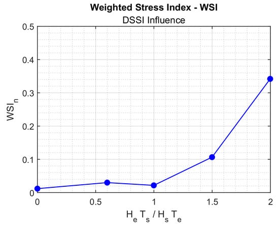
Figure 19. Bernal DLV weighted stress index vs. DSSI intensity parameter H_eT_s/H_sT_e.

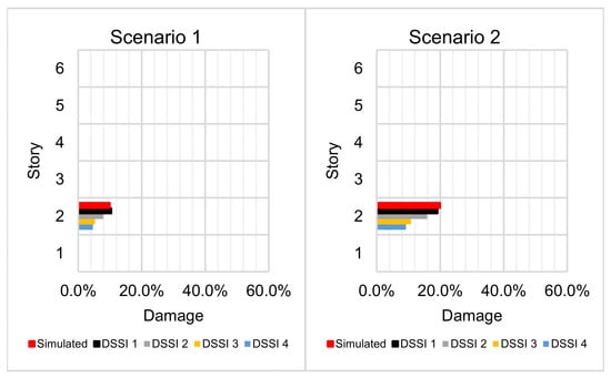
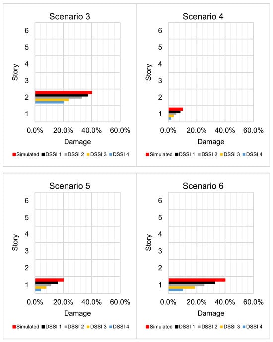
Figure 20. Damage identification summary of six scenarios under four soil flexibility levels.

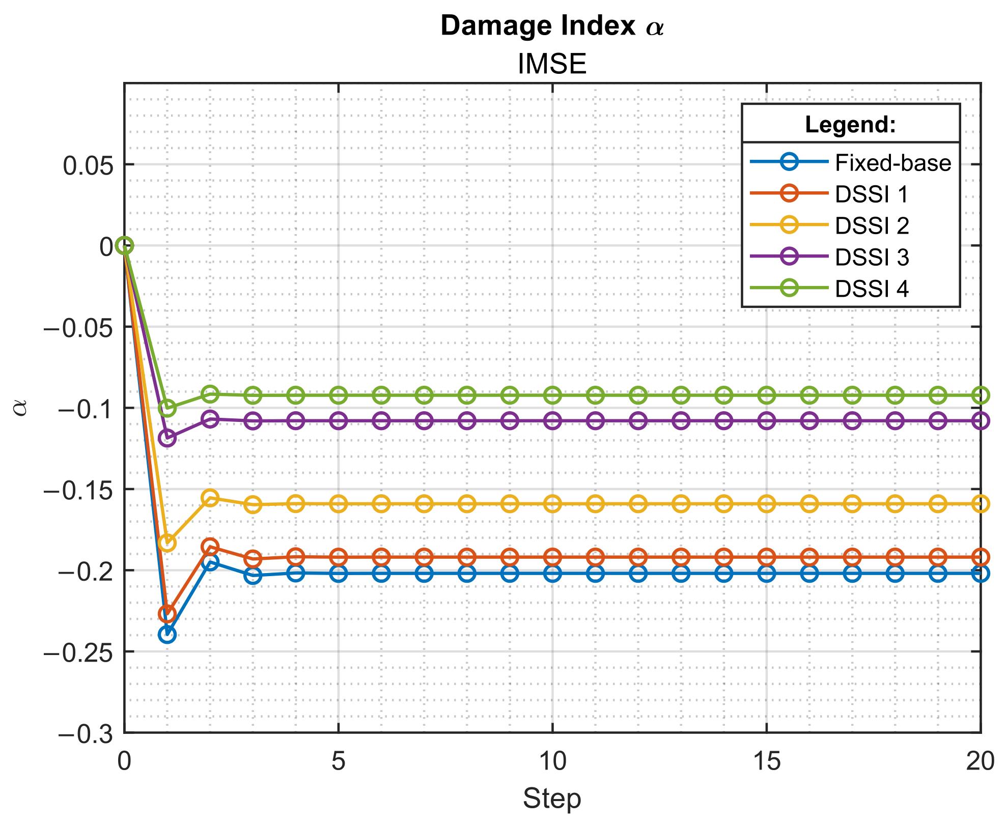
On the other hand, a comparison of the IMSE iteration results for the explored soil flexibilities is presented in Figure 21. In contrast to the fixed-base case, each softer scenario produced a damage index estimate smaller than that obtained from the simulation. It is important to note that DSSI had no effect on the convergence of the algorithm; in all cases, a stable value was reached after at most three iterations.

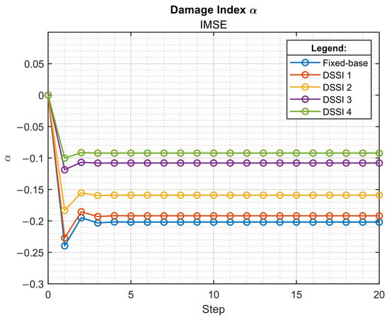
Figure 21. IMSE damage index for scenario no. 2 under four DSSI flexible base intensities.

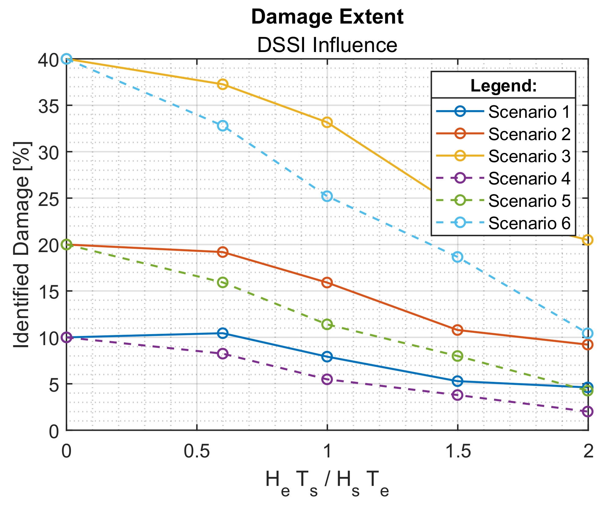
Finally, Figure 22 summarizes all the damage and DSSI scenarios explored; it presents the identified damage estimate as a function of DSSI intensity. Continuous lines represent scenarios in which damage was present on the second story, while dashed lines correspond to scenarios with damage on the first story. It can be observed that the dashed lines exhibit a steeper reduction in damage intensity; therefore, the effect of DSSI on damage identification is more pronounced for damage occurring in the lower story.

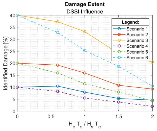
Figure 22. Damage identification methodology results versus DSSI intensity parameter H_eT_s/H_sT_e.

6. Conclusions

A VBSHM algorithm was proposed based on the well-established existing literature techniques with the goal of achieving Level 3 damage identification. The influence of DSSI on the damage detection algorithm was investigated through numerical simulations. Damage identification performance was evaluated for several damage scenarios and soil conditions. The VBSHM algorithm shows promising performance, accurately identifying damage presence, location, and extent, with no false positives or negatives in the explored scenarios—even when only the fundamental mode information is used. These results further motivate the need to understand its limitations under soft-soil conditions, which may be present and underestimated in practice.

Simulation results showed that damage identification algorithms may indeed be used under ambient vibrations whose frequency content differs from that of white-noise conditions, at least under the ideal imposed by the oversimplified model used for this first approach study. The performance of the used damage identification method under the influence of actual free-field ambient vibration recordings from the soft-soil Roma Norte site in Mexico City, together with kinematic DSSI, was comparable to that achieved under white-noise simulations. Further research directions may be explored by incorporating more rigorous and refined structural and soil modeling, accounting for measurement noise, considering uncertainties in soil and structural properties, and analyzing real experimental SHM recordings under the complexities of DSSI. An identified practical limitation on the input signal is that the excitation frequency content must be such that it effectively excites the fundamental mode of the system; otherwise, the structural response may be insufficient for reliable damage identification.

On the other hand, inertial DSSI was found to have a negative impact on damage identification performance under VBSHM. The proposed algorithm was still able to identify the presence and location of damage (Levels 1 and 2), but it performed less accurately in estimating the damage extent (Level 3). The results showed that the VBSHM algorithm increasingly underestimated the damage extent as the soil conditions became softer. The key practical implication of this result for real SHM systems is that damage extent can be underestimated if current VBSHM techniques are applied while ignoring the presence of DSSI. The magnitude of the error in the estimated damage intensity was found to depend on both the expected damage (in the absence of DSSI) and its location within the structure. In this regard, damage identification conclusions may be improved by quantifying the actual soil flexibility in the field, thereby providing insight into the likely uncertainty associated with current damage-extent estimates.

It is hypothesized that under softer soil conditions, the dynamic response of the building is dominated by so-called rigid-body motion, as a direct consequence of DSSI. From a structural dynamics perspective, soil flexibility causes the superstructure degrees of freedom to become dependent on the soil–foundation motion. The structural system, which consists of a series of elements with comparable stiffness, tends to behave as a single rigid body that is forced to translate and rock according to the motion of a second mechanism: the soil–foundation system. Because of this rigid-body motion, DSSI reduces the relative interstory displacements, and it is proposed that the VBSHM algorithm tends to underestimate the damage extent under these conditions.

It is assumed that additional signal processing—possibly combined with extra measurement points in the structure and/or its foundation—will be required to further improve the performance of VBSHM algorithms. In other words, using true structural response signals instead of the overall system response may be necessary to achieve robust damage identification. In this regard, future work could investigate applying an improved system identification step before damage identification, that is, to compensate for the soil flexibility and input the true structural modal properties to the VBSHM algorithm. Our insight is that this can be achieved with additional measurements in the foundation system and performing a spectral analysis like the one proposed by Stewart and Fenves [10] prior to the VBSHM procedure, to determine whether it improves performance.

If no additional measurements can be obtained—whether due to limited instrumentation budgets or other constraints—a practical idea of the present results would be to perform damage identification using the full system response signals and then correct the estimated damage extent by generating a plot like Figure 22. This correction could be made by referencing the identified damage from simulations using the design FEM model at different test damage scenarios calculated for different levels of the DSSI intensity parameter (H_eT_s/H_sT_e) corresponding to the site soil conditions, thus capturing some uncertainties on the real site conditions. In this sense, further research paths for further generalizing the results may include parametric simulations for key parameters that are expected to affect the relationship between soil flexibility and damage estimates, which include different building heights, the presence of asymmetries, numbers of degrees of freedom, and damage scenarios, to develop a set of robust damage-correction nomograms applicable to various building types and soft-soil conditions.

References

- Rytter, A. Vibrational Based Inspection of Civil Engineering Structures. Ph.D. Thesis, Department of Building Technology and Structural Engineering, Aalborg University, Aalborg, Denmark, 1993. [Google Scholar]
- Doebling, S.; Farrar, C.; Prime, M.; Shevitz, D. Damage Identification and Health Monitoring of Structural and Mechanical Systems from Changes in Their Vibration Characteristics: A Literature Review; Report LA-13070-MS; Los Alamos National Laboratory: Los Alamos, NM, USA, 1993.
- Terzi, V.G.; Manolis, G.D. Model reduction for structural health monitoring accounting for soil-structure-interaction. Maint. Manag. Life-Cycle Des. Perform. 2021, 17, 779–791. [Google Scholar] [CrossRef]
- Todorovska, M.I.; Niu, B.; Lin, G.; Cao, C.; Wang, D.; Cui, J.; Wang, F.; Trifunac, M.D.; Liang, J. A new full-scale testbed for structural health monitoring and soil–structure interaction studies: Kunming 48-story office building in Yunnan province, China. Struct. Control Health Monit. 2020, 27, e2545. [Google Scholar] [CrossRef]
- Sun, H.; Büyüköztürk, O. The MIT Green Building benchmark problem for structural health monitoring of tall buildings. Struct. Control Health Monit. 2018, 25, e2115. [Google Scholar] [CrossRef]
- Zar, A.; Hussain, Z.; Akbar, M.; Rabczuk, T.; Lin, Z.; Li, S.; Ahmed, B. Towards vibration-based damage detection of civil engineering structures: Overview, challenges, and future prospects. Int. J. Mech. Mater. Des. 2024, 20, 591–662. [Google Scholar] [CrossRef]
- Singh, T.; Sehgal, S. Damage identification using vibration monitoring techniques. Mater. Today Proc. 2022, 69, 133–141. [Google Scholar] [CrossRef]
- Zhang, C.; Mousavi, A.A.; Masri, S.F.; Gholipour, G.; Yan, K.; Li, X. Vibration feature extraction using signal processing techniques for structural health monitoring: A review. Mech. Syst. Signal Process. 2022, 177, 109175. [Google Scholar] [CrossRef]
- Farrar, C.R.; Worden, K. An introduction to structural health monitoring. Philos. Trans. R. Soc. A Math. Phys. Eng. Sci. 2007, 365, 303–315. [Google Scholar] [CrossRef]
- Stewart, J.; Fenves, G. System Identification for Evaluating Soil-Structure Interaction Effects in Buildings from Strong Motion Recordings. Earthq. Eng. Structrual Dyn. 1998, 27, 869–885. [Google Scholar] [CrossRef]
- Wolf, P.J. Dynamic Soil-Structure Interaction, 1st ed.; Prentice-Hall: Englewood Cliffs, NJ, USA, 1985. [Google Scholar]
- Fernández-Sola, L.R.; Castillo-Córdoba, S.E. Modificación de los parámetros modales debidos a los efectos de interacción dinámica suelo estructura. Ing. Investig. Y Tecnol. 2024, 25, 1–12. [Google Scholar] [CrossRef]
- Luco, J.; Trifunac, M.; Wong, H. Isolation of soil-structure interaction effects by full-scale forced vibration tests. Earthq. Eng. Struct. Dyn. 1988, 16, 1–21. [Google Scholar] [CrossRef]
- Trifunac, M.; Ebrahimian, M. Detection thresholds in structural health monitoring. Soil. Dyn. Earthq. Eng. 2014, 66, 319–338. [Google Scholar] [CrossRef]
- Murià Vila, D.; González Alcorta, R.; Espinosa Aranda, J. Efectos de Interacción Suelo-Estructura en la Respuesta Sísmica de un Edificio Instrumentado. In Report Instituto de Ingeniería, Geo-UNAM, V,2 N3, Universidad Nacional Autónoma de México, Instituto de Ingeniería; Dirección General de Bibliotecas de la UNAM: Ciudad de México, México, 1994; Available online: https://hdl.handle.net/20.500.14330/PER01000010354 (accessed on 18 May 2026).
- Dogan, T.P.; Erkan, I.H. Evaluation of the Nonlinear Seismic Responses of High-Rise Reinforced Concrete Buildings with Different Foundations and Structural Plans—Considering Soil-Structure Interactions. Buildings 2024, 14, 1686. [Google Scholar] [CrossRef]
- Farhad, A.A.A.; Aydın, E. Viscous Damper Optimization in Low-Rise Adjacent Buildings Exposed to Earthquakes by Considering the Soil-Structure Interaction. Buildings 2025, 15, 260. [Google Scholar] [CrossRef]
- Kir.il, M.S.; Ethemoglu, H. Effect of Soil–Structure Interaction on the Damage Probability of Multistory RC Frame Buildings with Shallow Foundations. Buildings 2025, 15, 624. [Google Scholar] [CrossRef]
- Juang, J.; Pappa, R. An eigensystem realization algorithm for modal parameter identification and model reduction. J. Guid. Control Dyn. 1985, 8, 620–627. [Google Scholar] [CrossRef]
- Bernal, D. Load vectors for damage localization. J. Eng. Mech. 2002, 128, 7–14. [Google Scholar] [CrossRef]
- Caicedo, J.; Dyke, S.; Jhonson, E. Natural Excitation Technique and Eigensystem Realization Algorithm for Phase I of the IASC-ASCE Benchmark Problem: Simulated Data. J. Eng. Mech. 2004, 130, 49–60. [Google Scholar] [CrossRef]
- Wang, S. Iterative modal strain energy method for damage severity estimation using frequency measurements. Struct. Control Health Monit. 2011, 20, 230–240. [Google Scholar] [CrossRef]
- Avilés, J. Análisis Sísmico de Sistemas Suelo-Estructura: Interacción en el modo Fundamental y los Modos Superiores. In Informe IIE/42/2843/I 02/F JAL; Instituto de Investigaciones Eléctricas: Cuernavaca, Mexico, 1991. [Google Scholar]
- Fernández Sola, L.R.; Avilés López, J. Efectos de interacción suelo-estructura en edificios con planta baja blanda. Ing. Sísmica 2008, 79, 71–90. [Google Scholar] [CrossRef]
- Kausel, E.; Whitman, R.; Morray, J.; Elsabee, F. The spring method for embedded foundations. Nucl. Energy Des. 1978, 48, 377–392. [Google Scholar] [CrossRef]
- Gazetas, G. Analysis of machine foundation vibrations: State of the art. Soil. Dyn. Earthq. Eng. 1983, 2, 2–42. [Google Scholar] [CrossRef]
- Gazetas, G. Foundation Vibrations, Foundation Engineering Handbook; Van Nostrand Reinhold: Nueva York, NY, USA, 1991. [Google Scholar]
- Sieffert, J.G.; Cevaer, F. Handbook of Impedance Functions; Ouest Editions: Rennes, France, 1995. [Google Scholar]
- Consejería Jurídica y de Servicios Legales de la Ciudad de México. Reglamento de Construcciones y Normas Técnicas Complementarias del Reglamento de Construcciones para el Distrito Federal; Gaceta Oficial del Gobierno de la Ciudad de México: Ciudad de México, México, 2024.
- Chopra, A.K. Dynamics of Structures: Theory and Applications to Earthquake Engineering, 5th ed.; Pearson: Hoboken, NJ, USA, 2017. [Google Scholar]
Disclaimer/Publisher’s Note: The statements, opinions and data contained in all publications are solely those of the individual author(s) and contributor(s) and not of MDPI and/or the editor(s). MDPI and/or the editor(s) disclaim responsibility for any injury to people or property resulting from any ideas, methods, instructions or products referred to in the content. |
© 2026 by the authors. Licensee MDPI, Basel, Switzerland. This article is an open access article distributed under the terms and conditions of the Creative Commons Attribution (CC BY) license.