


Abstract
Low-strain reflection testing is widely used for the rapid screening of pile integrity, but its interpretation still relies heavily on manual judgment. This study proposes a dual representation learning framework for classifying the integrity of building foundation piles from low-strain testing records. A dataset containing 1139 piles from engineering projects was established and divided into four integrity classes. Each record was represented in two complementary forms: structured features extracted from engineering parameters and waveform characteristics, and a redrawn waveform image generated from coordinate point data. Support vector machine (SVM), random forest (RF), and convolutional neural network (CNN) models were used as single modality baselines, and their performance was compared with that of a multimodal neural network (MNN) trained on paired structured and image inputs. The multimodal model achieved the highest overall accuracy on the main evaluation subset, reaching 84.65%, whereas the random forest achieved the best Macro-Recall and Macro-F1. This result suggests that multimodal fusion mainly improved overall robustness rather than consistently enhancing performance across all classes. Clearly intact piles and severely defective piles were easier to identify, whereas Class II remained the most difficult category because of its borderline signal characteristics. In the supplementary external validation set, the same ranking of model performance was observed, and the multimodal model achieved an accuracy of 85%. These results indicate that the proposed framework has strong potential for computer-assisted screening of building foundation piles.
1. Introduction
Pile foundations are widely used and are among the primary elements responsible for transferring building loads [1]. The quality and integrity of piles strongly influence the safety, durability, and long-term performance of the superstructure [2,3,4]. With continuing urbanization and the expansion of major civil engineering projects, the demand for reliable pile quality assessment has increased, both to safeguard structural safety and to support sustainable construction. At the same time, the growing use of very high-capacity foundations in supertall and long span structures has made integrity evaluation more challenging. Therefore, the assessment of pile integrity before a structure is put into service remains essential for improving safety, extending service life, and reducing the risk of foundation-related failure [5].
To meet this demand for accurate evaluation before commissioning, a range of pile integrity testing methods has been developed for engineering practice, including static load tests [6], high-strain dynamic tests [7], cross-hole sonic logging [8,9], and core drilling [10]. Under appropriate conditions, these methods can provide accurate results or direct physical evidence. However, they often involve higher cost, longer testing periods, or closer coordination with construction activities, which limits their applicability in rapid, large-scale surveys. By contrast, low-strain reflection testing (LST) is easy to implement, requires portable equipment, and involves relatively low testing cost, making it widely used for rapid on-site screening of pile defects [11,12]. Nevertheless, conventional interpretation of LST results still relies heavily on manual judgment. When datasets are large or signals are noisy and complex, this process becomes slow and labor intensive [13]. It may also introduce differences among analysts, thereby reducing consistency and reliability. These limitations highlight the need for more automated and data-driven approaches to the interpretation of low-strain reflection signals.
To overcome the limitations of manual interpretation, more intelligent and automated analysis is required. Machine learning (ML) is well suited to large, complex, and noisy datasets [14], and it has been widely applied in engineering fields such as image analysis [9], facility management [15], and the prediction of concrete properties [16,17,18]. In pile integrity testing, routine field inspections generate large volumes of data, yet much of this information remains underused because interpretation still depends heavily on experience and can be subjective [5]. Motivated by this gap, recent studies have explored ML-based interpretation of LST signals. Some approaches train classifiers using engineered features extracted from the waveform or its spectrum for rapid screening, whereas others learn directly from raw signal sequences using deep models to reduce reliance on manual feature design [19,20,21]. For example, Cui et al. [20] developed a computer-assisted workflow that combines signal processing with machine learning to screen large numbers of reflectograms and flag suspected piles for expert review. In parallel, other studies have used reflectogram images, or related transformed plots, as inputs to convolutional neural network models to improve recognition under noisy conditions and across multiple defect patterns [22,23,24]. For example, Wu et al. [24] trained a convolutional neural network on plot images to identify multiple defect patterns in noisy low-strain records. These studies indicate strong potential for automated screening. However, the same test record is often stored in different formats across projects, and many models are designed for only one format, which limits portability and may reduce robustness when that single input is degraded. Low-strain reflection data are typically recorded either as waveform images or as coordinate points, corresponding to image and structured data modalities, respectively. This dual representation makes model selection less straightforward and may increase prediction errors, especially when one modality is noisy or incomplete.
To address this challenge, this study focuses on the integrity classification of building foundation piles using LST. Rather than treating plotted waveforms and structured descriptors as interchangeable inputs, a dual representation fusion strategy is proposed to jointly learn from the same reflectogram in two complementary forms: engineered structured features and waveform images. This design better reflects practical data management in foundation inspection, where the same test record is often archived both as coordinate points and as report ready plots. On this basis, support vector machine (SVM), random forest (RF), and convolutional neural network (CNN) models are used as single representation baselines, and their performance is compared with that of a multimodal neural network (MNN) trained on paired inputs. Finally, supplementary external validation using model pile records and additional intact field piles is conducted to examine the robustness of the proposed framework across different scenarios.
2. Methodology
This section presents the models used to classify pile integrity from LST data. Two conventional models, SVM and RF, were implemented in Python (version 3.9.13; Python Software Foundation, Wilmington, DE, USA) using scikit-learn and were trained on structured features. The CNN baseline and the MNN were implemented using TensorFlow with the integrated Keras API (version 2.15.0; Google LLC, Mountain View, CA, USA). The CNN baseline was trained on waveform images, whereas the MNN was developed to fuse structured and image inputs within a unified framework.
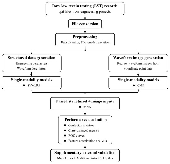
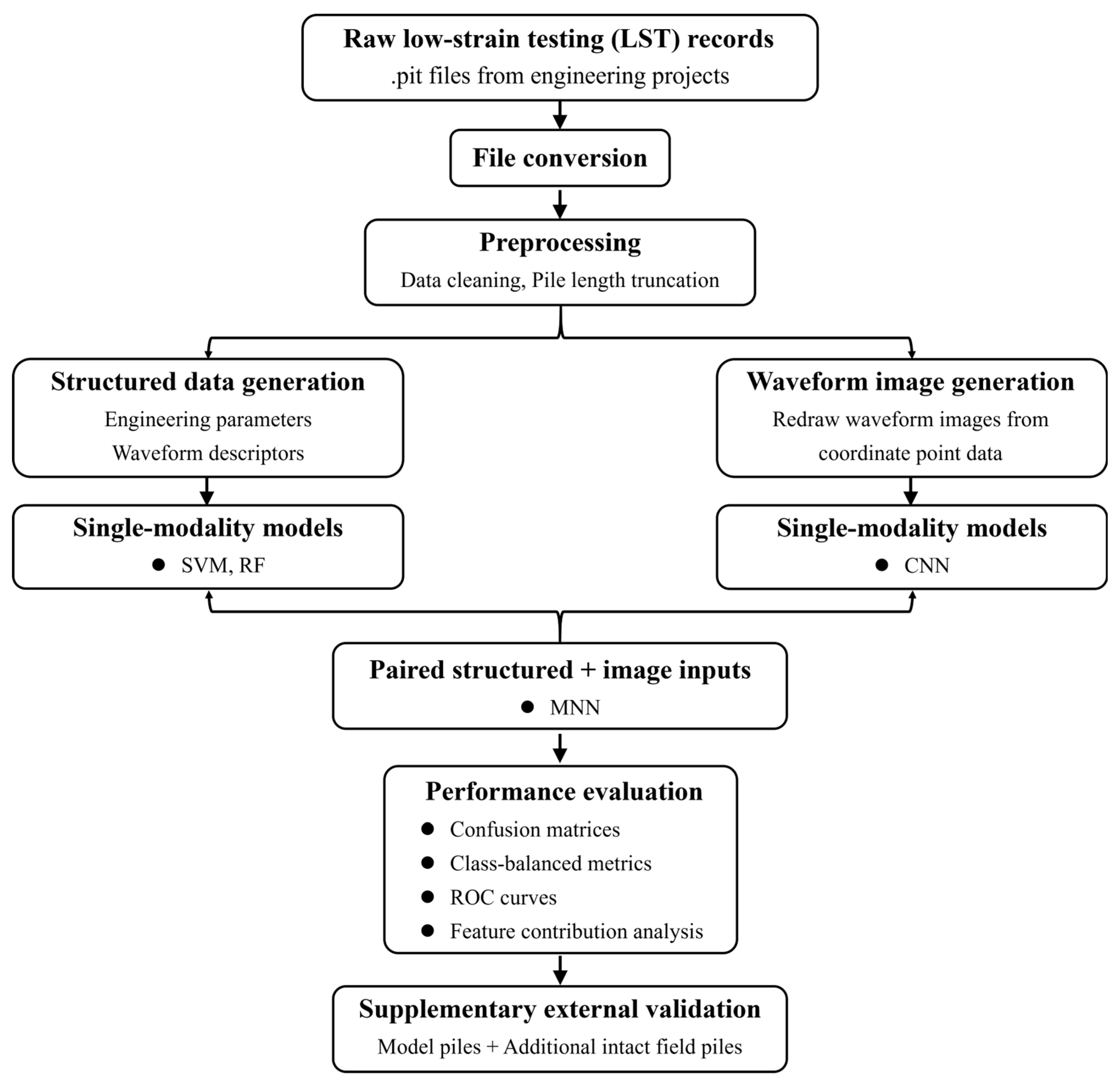
The overall workflow of this study is summarized in Figure 1. The raw LST records were acquired using a PIT pile integrity tester (model C2-070; Pile Dynamics, Inc., Cleveland, OH, USA) and were first exported from the proprietary .pit format using PIT-W software (version 2009; Pile Dynamics, Inc., Cleveland, OH, USA). After pile length truncation and data cleaning, two paired representations were generated for each pile record: structured descriptors extracted from engineering parameters and waveform characteristics, and waveform images redrawn from coordinate point data. The structured data were used to train SVM and RF models, whereas the waveform images were used to train the CNN model. The paired structured and image inputs were further integrated in the MNN for multimodal classification. Finally, the models were evaluated using confusion matrices, class-balanced metrics, ROC curves, feature contribution analysis, and supplementary external validation.
Figure 1.
Flowchart of the proposed methodology for multimodal pile integrity classification using LST record.
2.1. Support Vector Machine (SVM)
SVM is a supervised classification algorithm that separates classes by identifying a decision boundary that maximizes the margin between them. To handle nonlinear classification problems, a kernel function can be used to map the input features into a higher dimensional space in which the classes are more easily separable. In this study, SVM was implemented as a structured data baseline. The final model adopted a radial basis function (RBF) kernel with and , as determined by grid search with five-fold cross validation.
2.2. Random Forest (RF)
RF is an ensemble learning method that constructs multiple decision trees from bootstrap resampled training subsets and combines their outputs through majority voting for classification. By introducing randomness in both sample selection and feature selection, RF can effectively reduce variance and improve robustness compared with a single decision tree. In this study, RF was used as a structured data baseline to classify pile integrity based on engineered descriptors extracted from low-strain reflection records. The final model consisted of 200 trees, with a maximum depth of 10, a minimum of 10 samples required for splitting, a minimum of 2 samples per leaf node, and the number of maximum features set to the square root of the total feature number.
2.3. Convolutional Neural Network (CNN)
CNN is a deep learning architecture widely used in image recognition and pattern classification tasks [23]. It consists of multiple layers, including convolutional layers, pooling layers, and fully connected layers. Convolutional layers apply local filters to extract spatial features from the input data, whereas pooling layers reduce dimensionality and improve robustness to noise and variation. Fully connected layers integrate the extracted features to perform classification or regression. CNN is particularly effective for image based data because it can automatically learn hierarchical feature representations without requiring manual feature engineering. The architecture of the CNN model used in this study is summarized as follows.
- (i)
- Convolutional layers: Three convolutional modules were used, with 32, 64, and 128 filters, respectively. Each convolution used a kernel and the ReLU activation function.
- (ii)
- Pooling layers: A max pooling layer followed each convolutional module to progressively reduce the spatial dimensions while preserving salient features.
- (iii)
- Fully connected layers: The flattened feature maps were fed into a fully connected layer with 512 units, followed by a Softmax output layer that generated probability distributions over the four target classes.
The model was trained using the categorical cross entropy loss function, which quantifies the discrepancy between the predicted probabilities and the ground truth labels. The Adam optimizer was adopted with its default hyperparameters, namely a learning rate of , , and [25]. A total of 150 epochs was used, with a batch size of 3 to balance training efficiency and GPU memory constraints. Data augmentation was performed dynamically through a generator to prevent memory overflow and improve model generalization. The accuracy and loss curves of both the training set and the validation set were continuously monitored to evaluate model performance. All experiments were implemented using the TensorFlow framework [26].
2.4. Multimodal Neural Network (MNN)
This study proposes an MNN that fuses two paired representations derived from the same low-strain test record: a waveform image and a structured feature vector. Although both inputs originate from the same reflectogram, they preserve complementary information at different levels of abstraction. The image branch retains the global morphology and local visual patterns of the waveform, whereas the structured branch encodes engineering information related to pile geometry and reflection characteristics. Therefore, a dual branch late fusion architecture was adopted to exploit this representational complementarity within a unified framework.
- (i)
- Image feature extraction branch: The image feature extraction branch consists of an input layer, a convolutional module, and a fully connected layer. The input layer receives red, green, and blue (RGB) images with a resolution of . The convolutional module includes a first convolutional layer with 32 filters of size and ReLU activation, producing feature maps of , followed by a max pooling layer with a stride of 2 that reduces the output to . A second convolutional layer with 64 filters of size is then applied, generating feature maps of . The fully connected layer compresses the flattened features into a 128 dimensional vector, and a dropout rate of 0.5 is used to mitigate overfitting.
- (ii)
- Structured data branch: The structured data branch consists of an input layer and a feature enhancement module. The input layer receives a five-dimensional vector of standardized engineering parameters. The feature enhancement module contains a first fully connected layer with 64 neurons and ReLU activation, followed by batch normalization, and a second fully connected layer with 128 neurons and ReLU activation, followed by a dropout rate of 0.5.
- (iii)
- Feature fusion and classification module: The feature fusion and classification module consists of a concatenation layer and a joint decision layer. The concatenation layer merges the 128-dimensional feature vector from the image branch with the 128-dimensional feature vector from the structured data branch, forming a unified 256-dimensional representation. The joint decision layer includes a fully connected layer with 128 neurons and ReLU activation, followed by a dropout rate of 0.5, and an output layer with four neurons using a Softmax classifier to predict the four pile condition categories.
3. Dataset Description
This section describes the dataset used for model development and evaluation. It is organized into four subsections. First, the source of the low-strain testing records and the integrity class labels are introduced. Second, the raw data format and preprocessing workflow are described, including file format conversion and pile length truncation. Third, the three data modalities used as model inputs are presented. Finally, the data split protocol and reproducibility settings are summarized to support transparent model evaluation.
3.1. Data Source and Class Labels
The dataset was collected from field low-strain reflection tests conducted for pile integrity evaluation in real engineering projects. The raw test records were stored in the proprietary .pit format of the testing instrument, and the integrity labels were assigned by qualified testing engineers and documented in formal inspection reports, thereby providing reliable ground truth labels for model training and evaluation.
A total of 1139 piles were included and categorized into four classes: 567 piles in Class I, 138 piles in Class II, 170 piles in Class III, and 264 piles in Class IV. Classes I and II were considered serviceable. Class III piles required reinforcement and retesting, or further verification through design calculations before they could be regarded as usable. Class IV piles were considered unserviceable and had to be demolished and replaced with newly cast piles. For model development, the dataset was further processed into three modalities as input sets for different machine learning models.
3.2. Raw Data Format and Preprocessing Workflow
3.2.1. File Format Conversion
In engineering practice, the instrument output was stored in a proprietary .pit format. Because .pit files could not be directly used in most machine learning workflows, they were opened using Pit-W software and exported to Word format. In the exported Word files, each waveform was stored as a set of coordinate points containing 256 recorded data points. Python scripts were then used to batch extract the waveform data and basic pile information and convert them into machine readable tables for subsequent processing.
3.2.2. Pile Length Truncation
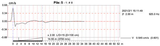
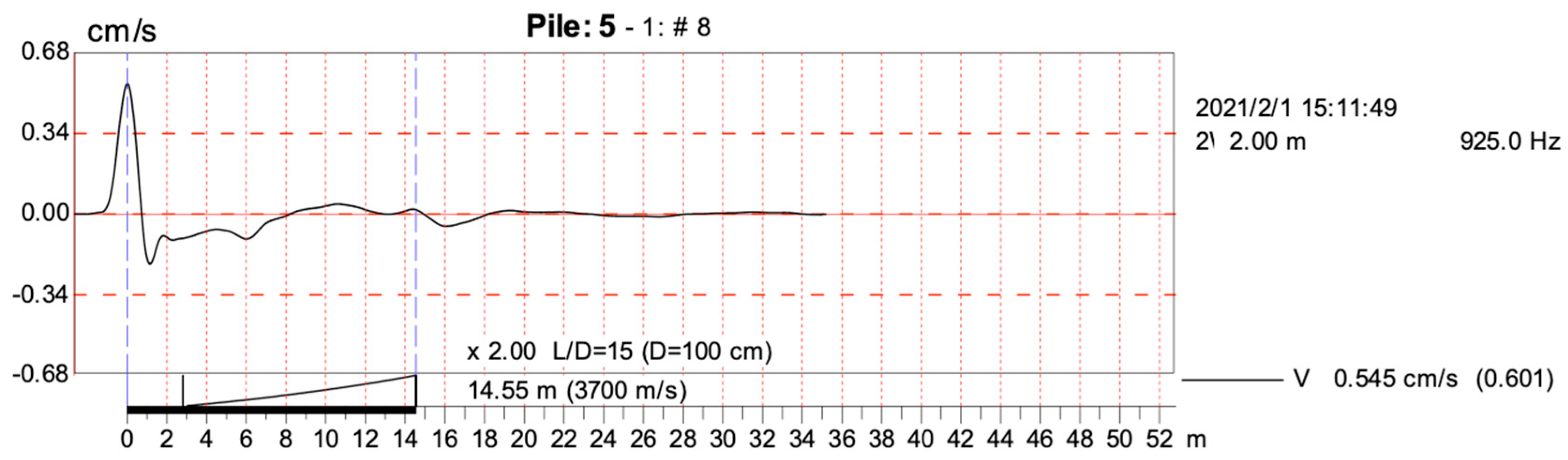
To minimize errors caused by inconsistent data selection, a pile length truncation method was adopted. In Figure 2, the black solid curve represents the measured velocity response exported from PIT-W software, the red dashed lines are reference gridlines generated by the software, and the “#” symbol denotes the waveform record number. As indicated by the blue dashed lines, only the curve segment corresponding to the effective pile length range was extracted for analysis, thereby avoiding the risk of computing features outside the valid pile length range. In implementation, the truncation window was determined based on the impact response and the expected travel duration within the pile length range, and the corresponding segment was then extracted.
Figure 2.
Representative raw LST waveform and pile length truncation range.
3.3. Data Modalities for Model Inputs
3.3.1. Modality I: Structured Data
The first modality was structured data, which was constructed by extracting representative features from low-strain waveforms stored as coordinate points and combining them with basic pile information. Based on engineering practice, the core inputs included pile diameter, pile length, assumed wave velocity, waveform amplitude difference, and peak-related descriptors, while the integrity class was used as the target label. Peak locations were identified using the find_peaks function. The waveform amplitude difference was defined as the difference between the amplitude of the first major peak and the average amplitude of its adjacent valleys. In addition, an extra feature was introduced to quantify peak distribution within the pile length range. Specifically, the numbers of peaks exceeding amplitude thresholds of 0.03, 0.04, 0.05, 0.06, and 0.07 cm/s were recorded as a sequence (a, b, c, d, e). For example, Class I piles typically showed sequences such as (1, 0, 0, 0, 0) or (0, 0, 0, 0, 0), whereas Class IV piles often showed sequences such as (5, 4, 3, 2, 1). This sequence feature provided a quantitative description of peak distribution and improved class separability.
In low-strain reflectograms, reflections appear as waveform peaks, and feature extraction is commonly performed within the effective time window bounded by the pile head reflection and the pile toe reflection. Because defect-induced impedance changes introduce additional reflected components, the distribution and prominence of local waveform peaks within this window can provide useful information on signal irregularity. In this study, the numbers of waveform peaks identified under several amplitude thresholds were used to characterize such changes. This treatment reduced reliance on a single threshold and provided a more stable description of waveform complexity [20].
3.3.2. Modality II: Image Data
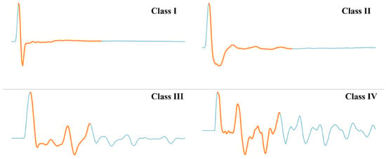
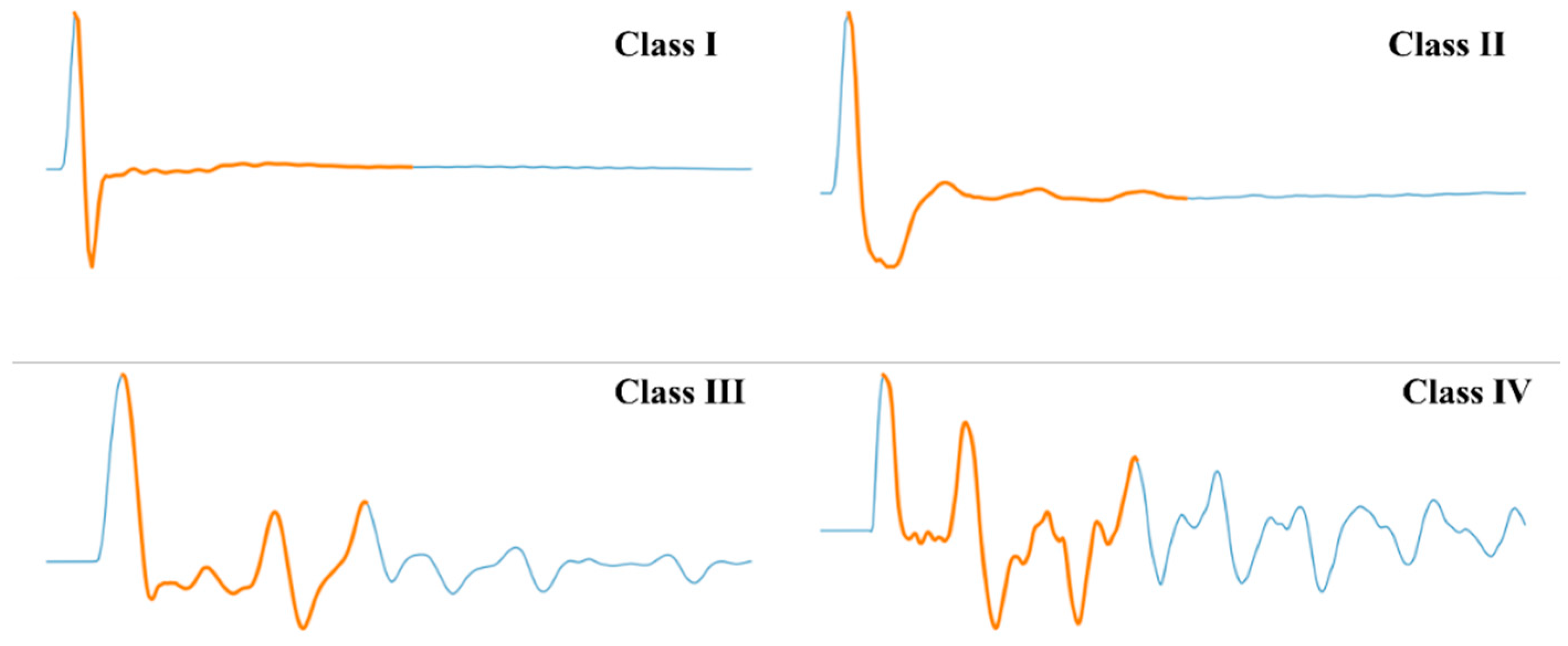
The second modality was image data, in which low-strain curves were represented as waveform images. The inputs for the neural network model were generated by redrawing each low-strain reflection curve from its coordinate points. To enable the model to capture the location of the effective pile length range while preserving the overall waveform shape, an overlay plotting scheme was adopted to highlight the effective interval within the same plot. Representative examples of the four integrity classes are shown in Figure 3. In these images, the orange curve segments indicate the effective pile length range retained for subsequent feature extraction and image based model input, whereas the blue curve segments represent waveform portions outside the selected range. All images were resized to a uniform resolution of 308 × 852 pixels and converted into RGB tensors for model input. To reduce overfitting under limited training data, data augmentation was applied during CNN training, including pixel rescaling and simple geometric transformations, and 20% of the training set was used as the validation split.
Figure 3.
Representative waveform images of the four pile integrity classes used as inputs to the neural network model.
3.3.3. Modality III: Multimodal Data
The third modality was multimodal data, which were obtained by combining the structured and image modalities. Each pile sample therefore contained paired inputs, including a structured feature vector and its corresponding waveform image. Cross-modal pairing was ensured by using the stake number, namely the pile ID, to map image files to the structured records.
3.4. Data Split and Reproducibility Settings
The data split protocol and the final model settings used in this study are summarized in Table 1. For the structured data models, the dataset was divided into training and testing subsets at a ratio of 8:2 using a fixed random seed (random_state = 42), and five-fold cross-validation was used for hyperparameter tuning. The structured features were standardized for SVM, whereas RF was trained on the original feature scale. For the CNN model, all waveform images were resized to a unified input size, and 20% of the training images were used for validation through on the fly data augmentation. For the multimodal model, each structured sample and its corresponding waveform image were paired by pile ID and kept aligned during data splitting and training.
Table 1.
Hyperparameter search space and final model settings of the four models.
4. Performance Evaluation Metrics
Model performance was evaluated using a set of complementary metrics. Because the dataset was moderately imbalanced across the four integrity classes, overall accuracy alone was not considered sufficient. In addition to accuracy, Macro-Precision, Macro-Recall, Macro-F1, and balanced accuracy were used to provide a more balanced assessment of model performance [27]. Accuracy was defined as
where denotes the number of correctly classified samples in class , and is the total number of samples. For class , precision and recall were calculated as
where and denote the false positive and false negative samples in class , respectively. The corresponding F1 score was calculated as
The macro averaged metrics were then obtained by averaging the corresponding values across all classes:
Balanced accuracy was defined as the arithmetic mean of the recall values across all classes:
In the present multiclass setting, balanced accuracy was numerically identical to Macro-Recall. In addition, confusion matrix heatmaps were used to visualize the distribution of classification errors across classes. One versus rest receiver operating characteristic (ROC) curves and the corresponding area under the curve (AUC) values were used to assess the separability of each class. Finally, learning curves were used to examine training behavior and generalization performance. For SVM and RF, the learning curves show how training accuracy and validation accuracy changed as the number of training samples increased. For CNN and the proposed multimodal network, the loss and accuracy curves of the training and validation sets were tracked over epochs to assess convergence behavior and potential overfitting. To complement overall accuracy under class imbalance, class-balanced summary metrics were also used in the model comparison, and the corresponding results are presented together with the confusion matrix analysis in Section 5.2.
5. Results and Discussion
This section presents the classification performance of the four models from complementary perspectives. The analysis first examines the training behavior and learning curves to evaluate convergence and potential overfitting. It then compares the prediction results using confusion matrices, class-balanced evaluation metrics, and ROC curves. Finally, feature contribution and supplementary external validation are discussed to interpret the model behavior and assess its preliminary robustness.
5.1. Training Behavior and Learning Curves
The training behavior was analyzed separately for the structured data models and the deep learning models because their input forms and optimization processes differ. For SVM and RF, learning curves were used to examine the effect of training set size on model generalization. For CNN and MNN, training and validation accuracy and loss curves were monitored over epochs to evaluate convergence behavior and possible overfitting.
5.1.1. Learning Curves of Structured Data Models
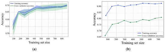
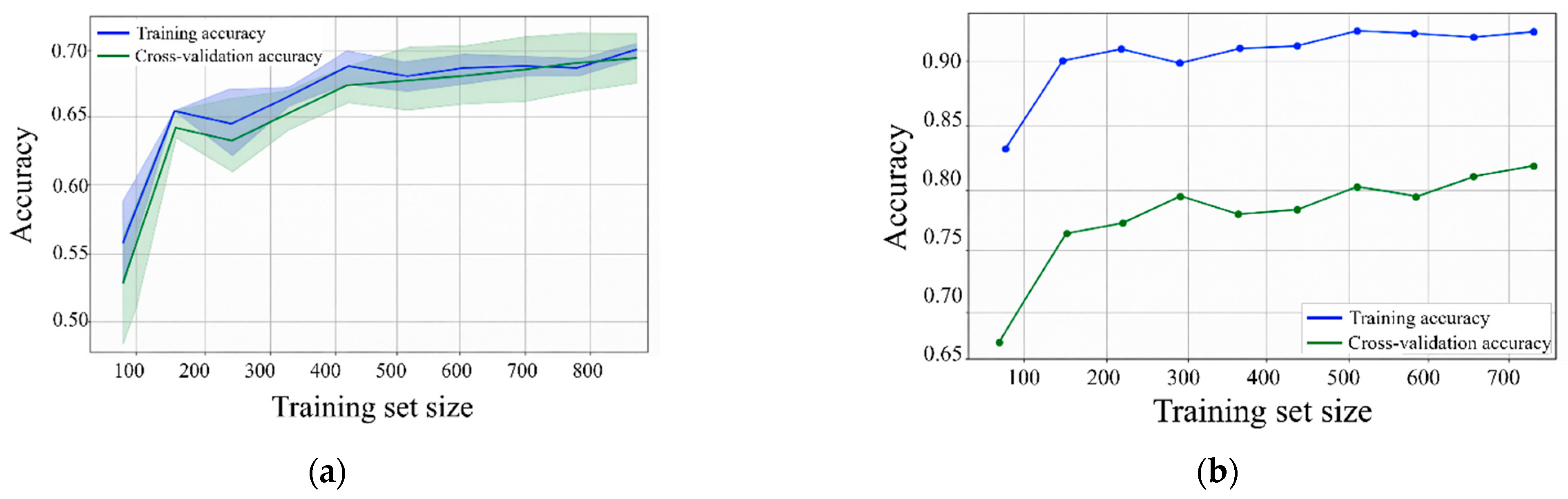
Figure 4a,b illustrates the learning behavior of the two feature-based models as a function of training set size. In Figure 4a, the SVM exhibits a typical convergence pattern: both the training score and the cross-validation score improve steadily, and the gap between them narrows significantly as the number of training samples increases. This decreasing divergence indicates that the model generalizes well and does not suffer from severe overfitting. However, both curves gradually approach a plateau at larger sample sizes. This saturation helps explain the residual classification errors discussed in later sections and suggests that feature-based decision boundaries are insufficient to fully resolve the ambiguity of borderline defect classes, particularly Class II. In contrast, the RF learning curves in Figure 4b maintain a noticeable gap between training performance and validation performance across all sample sizes. This divergence reflects the stronger flexibility of the ensemble model in fitting the training data, but it also indicates a larger variance component. More importantly, the validation accuracy reaches a plateau without converging toward the training level, suggesting an inherent limitation in feature separability. This result indicates that simply increasing the number of training samples cannot eliminate the underlying overlap among borderline cases. This finding is consistent with the confusion matrix results and further confirms that the generalization gap largely reflects the intrinsic difficulty of distinguishing intermediate integrity classes.
Figure 4.
Learning curves of the structured data models for pile integrity classification: (a) SVM; (b) RF.
5.1.2. Training Dynamics of Deep Models
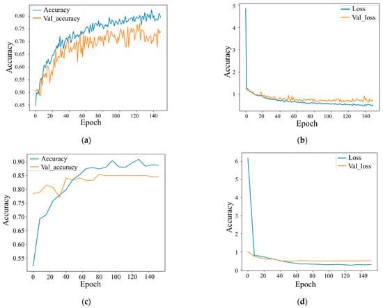
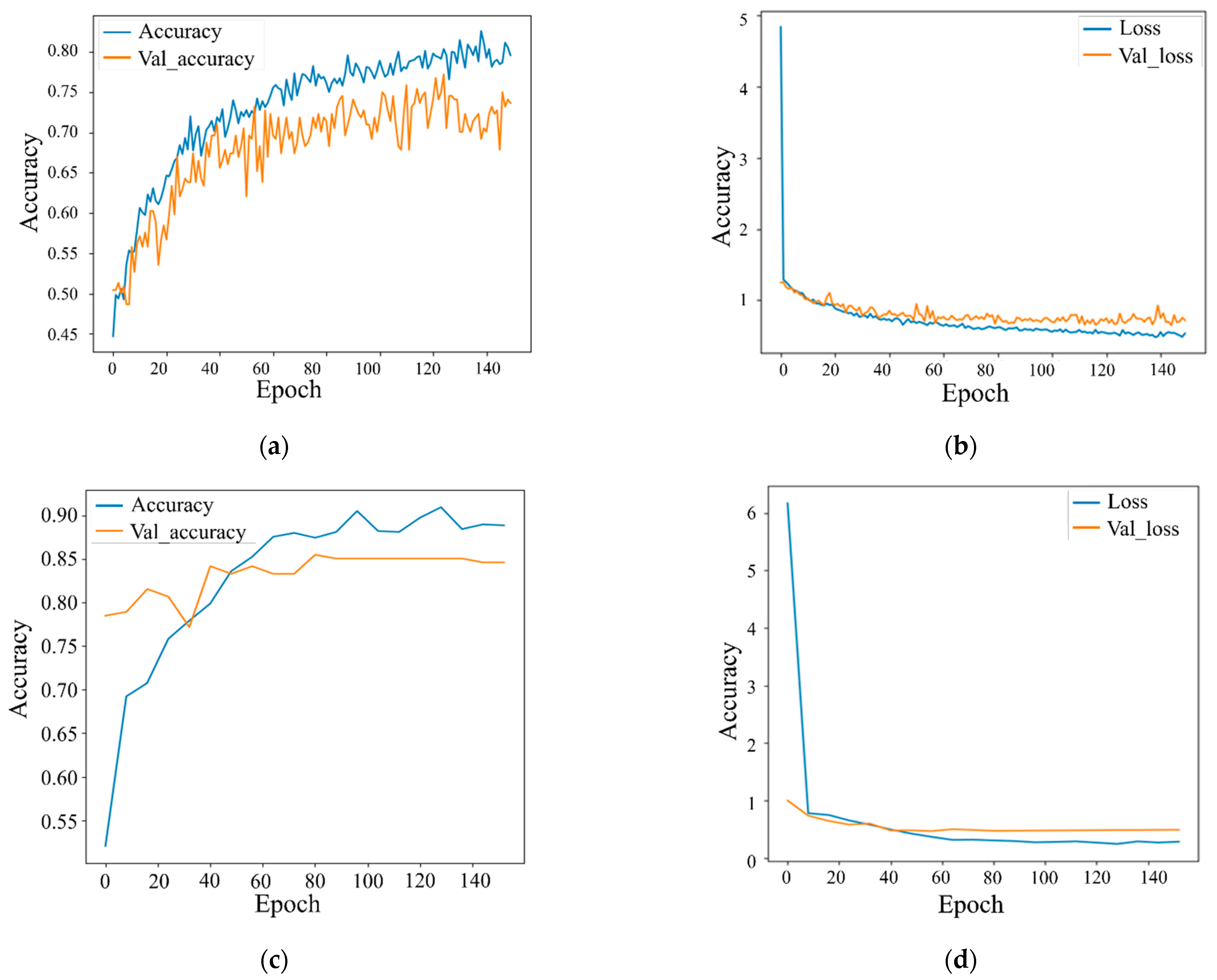
Figure 5 summarizes the optimization behavior and generalization trends of the deep models. For the CNN model, the final training accuracy and validation accuracy were approximately 0.80 and 0.74, respectively, while the final training loss and validation loss were approximately 0.50 and 0.70, respectively. The training accuracy increased rapidly during the early epochs and then continued to improve with modest gains, whereas the validation accuracy increased more slowly and showed noticeable fluctuations. Meanwhile, the training loss decreased continuously and stabilized at a lower level, while the validation loss remained higher and fluctuated around approximately 0.70 at the final stage. This divergence between the training and validation curves indicates a persistent generalization gap. It suggests that relying only on waveform images makes the CNN more sensitive to local noise, plotting variations, and limited image diversity in the reflectogram dataset. For the MNN model, the final training accuracy and validation accuracy were approximately 0.89 and 0.85, respectively, and the final training loss and validation loss were approximately 0.33 and 0.52, respectively. The accuracy curves increased rapidly during the early training stage and then gradually stabilized, with the validation accuracy plateauing at a relatively high level. The loss curves also decreased sharply at the beginning and then approached a stable state. Although a moderate gap between the training and validation loss remained, the validation accuracy curve was smoother and more stable than that of the CNN. This convergence behavior indicates that the integration of structured descriptors and waveform images helped improve learning stability and reduced the instability associated with using image inputs alone. These observations are consistent with the superior overall performance of the MNN in the subsequent classification evaluation.
Figure 5.
Training and validation curves of the deep models for pile integrity classification: (a) CNN accuracy; (b) CNN loss; (c) MNN accuracy; (d) MNN loss.
5.2. Confusion Matrix Analysis
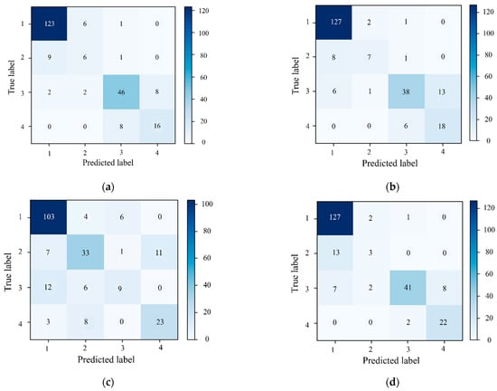
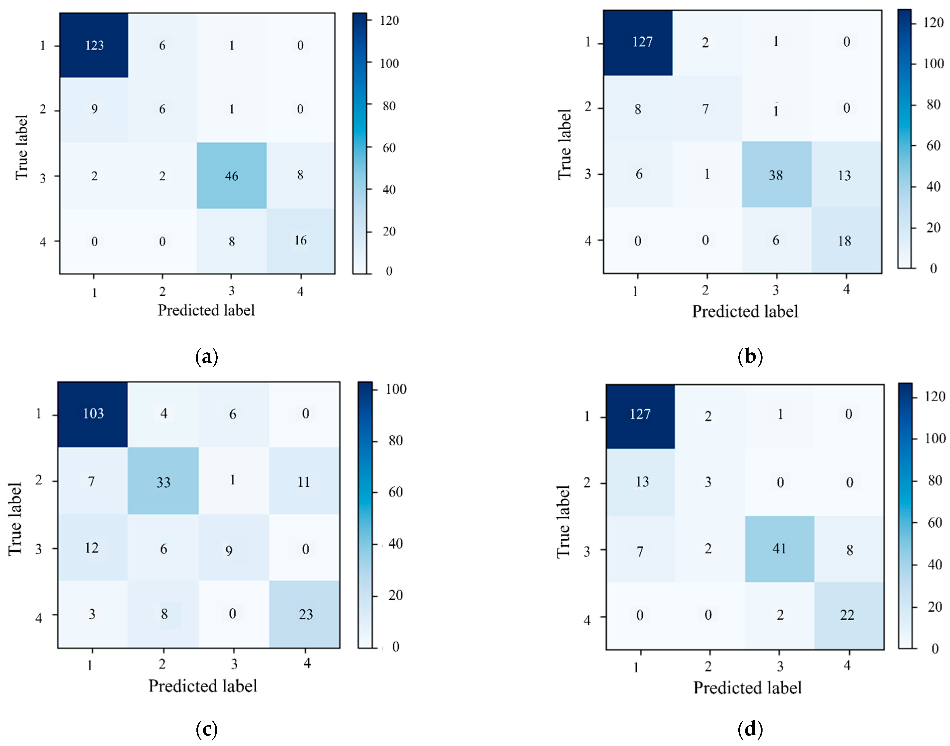
Figure 6 compares the prediction behavior of the four models across the integrity classes. For the structured data baselines, both SVM (Figure 6a) and RF (Figure 6b) achieve high recall for Class I, reaching 94.62% and 97.69%, respectively, which indicates reliable recognition of clearly serviceable piles. However, Class II remains challenging for both models, with substantially lower recall values of 37.50% for SVM and 43.75% for RF. In both confusion matrices, the dominant error is the misclassification of Class II as Class I, involving nine cases for SVM and eight cases for RF. This result suggests that mildly defective piles are often categorized as sound piles when the decision boundaries rely only on the current set of structured descriptors. In addition to Class II, persistent confusion is also observed between Class III and Class IV, which is important in practice because these classes may require different engineering treatments. The SVM model shows nearly symmetrical errors, with eight cases of Class III misclassified as Class IV and eight cases of Class IV misclassified as Class III. For RF, the dominant error source shifts to Class III samples being misclassified as Class IV, involving 13 cases. These results indicate that the boundary between repairable piles and structurally deficient piles is still not sufficiently resolved by the current structured feature set, likely because the associated attenuation and reflection patterns remain similar under complex field conditions [28].
Figure 6.
Confusion matrices showing sample counts for four class pile integrity classification on the evaluation subset: (a) SVM; (b) RF; (c) CNN; (d) MNN.
The CNN based only on image inputs (Figure 6c) further highlights the limitations of relying solely on visual waveform representations, with the overall accuracy decreasing to 74.34%. Its main weakness appears in Class III, for which the recall is only 33.33% (nine out of 27 cases). Many of these samples are instead assigned to Class I (12 cases) or Class II (six cases). In addition, the misclassification of Class II as Class IV, involving 11 cases, suggests that the visual mapping from waveform morphology to ordered integrity grades remains unstable. This result implies that the CNN is more sensitive to plotting style, local noise, and limited image diversity, and that stronger regularization and more robust data augmentation may be needed to improve generalization [29,30]. By contrast, the MNN (Figure 6d) shows better overall robustness by combining paired structured and visual representations. In particular, Class I retains high recall, and the recognition of Class IV is strengthened. The high precision achieved for Class III, reaching 93.18%, also suggests that the model is effective in suppressing spurious defect-related assignments. Nevertheless, the recall of Class II remains low at 18.75%, indicating that borderline defects are still strongly coupled with Class I even after multimodal fusion. Therefore, the advantage of the MNN should be understood as an improvement in overall robustness and in the discrimination of extreme classes, rather than as a complete resolution of the ambiguity associated with Class II.
To complement the above confusion matrix analysis under class imbalance, the models are further compared using the class-balanced summary metrics listed in Table 2. As shown in Table 2, the MNN achieves the highest overall accuracy, whereas RF yields the best Macro-Recall and Macro-F1. This comparison indicates that multimodal fusion improves overall classification performance, but its advantage is not uniform across all classes, especially for the borderline Class II category.
Table 2.
Summary of class-balanced evaluation metrics on the evaluation subset.
5.3. ROC and AUC Analysis
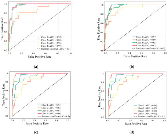
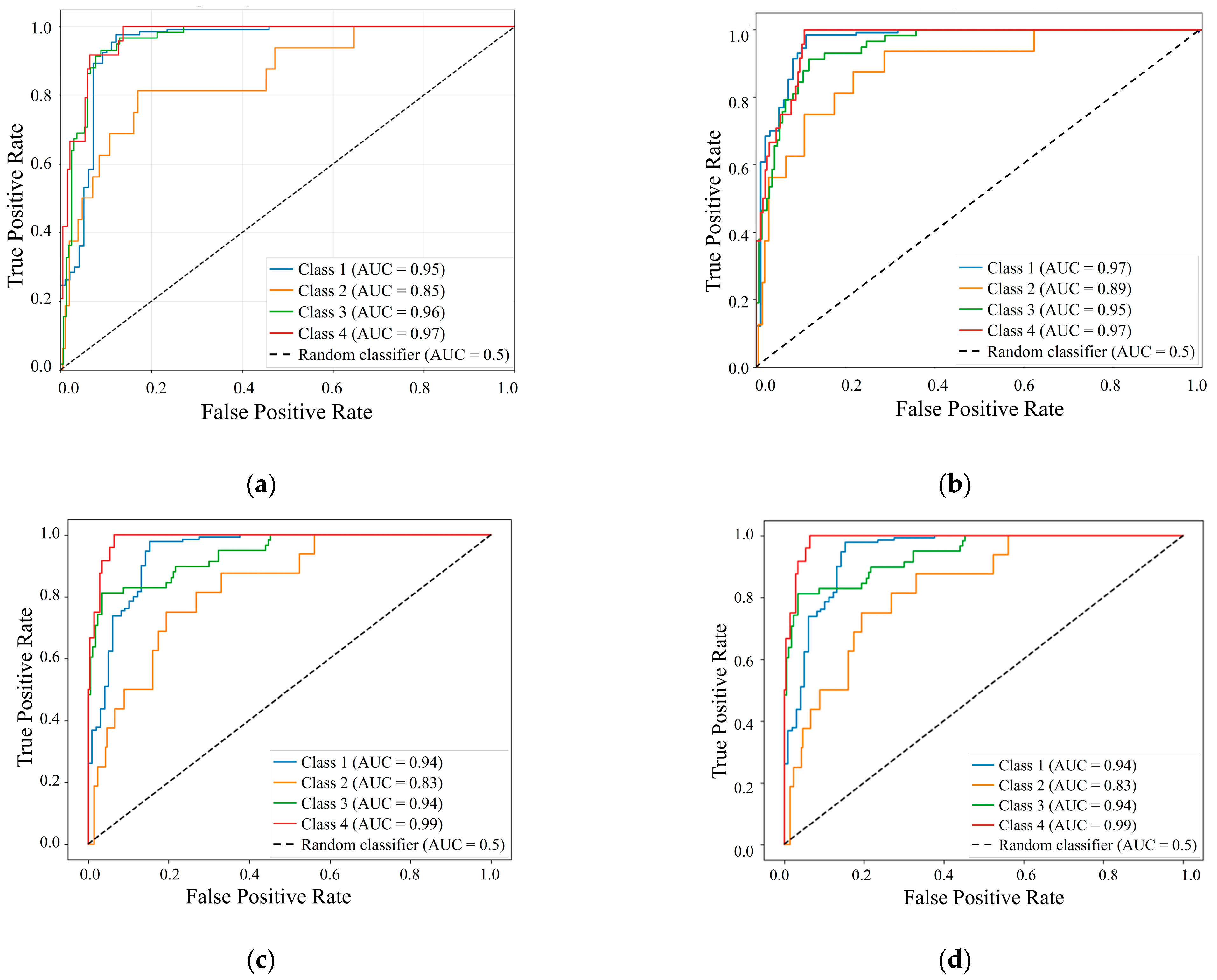
Beyond overall accuracy, one versus rest ROC curves provided further insight into the separability of individual classes (Figure 7). As reflected by the AUC values, the models achieved better performance in classifying clearly defined states, namely intact piles and severely defective piles, while showing relatively lower discriminative ability for intermediate categories. Figure 7a illustrates the ROC performance of the SVM model. The model achieved high AUC values of 0.95, 0.96, and 0.97 for Classes I, III, and IV, respectively, demonstrating strong discriminative ability for clearly intact piles and piles with significant defects. However, a noticeable decline in performance was observed for Class II, with an AUC of 0.85. This reduction suggests that the subtle reflected signal characteristics associated with slight defects are more easily masked by signal attenuation and noise, making them difficult to distinguish from adjacent integrity categories. Figure 7b presents the ROC curves for the RF model, which yielded AUC values of 0.97, 0.89, 0.95, and 0.97 for Classes I to IV, respectively. Similar to the SVM results, RF maintained high separability for intact piles and severely defective piles, whereas Class II remained the most challenging category, with an AUC of 0.89. Notably, RF showed a slight improvement in the separability of Class II compared with SVM. This improvement likely arises from the ensemble nature of RF, which is more capable of capturing nonlinear interactions among engineered features [31]. However, the persistent performance gap between Class II and the other categories underscores the intrinsic difficulty of delineating the boundary of slight defects using feature-based approaches.
Figure 7.
One versus rest ROC curves of the four models for pile integrity classification: (a) SVM; (b) RF; (c) CNN; (d) MNN.
Following the assessment of models based on structured numerical data, namely SVM and RF, Figure 7c illustrates the ROC performance of the CNN model. Although the CNN achieved exceptional separability for the most distinct category, namely Class IV, with a near perfect AUC of 0.99, and also showed strong performance for Classes I and III, both with an AUC of 0.94, it did not resolve the bottleneck associated with Class II, for which the AUC was 0.83. This decline in performance is consistent with the confusion matrix results, in which borderline defects were frequently misclassified into adjacent grades. These results suggest that when the model relies only on visualized reflectograms, the visual signatures of slight defects are less stable and are highly sensitive to plotting variations and local noise. Finally, Figure 7d presents the ROC performance of the MNN, which integrates both structured numerical data and waveform images. The MNN achieved AUC values of 0.94, 0.83, 0.94, and 0.99 for Classes I to IV, respectively. These results indicate that multimodal fusion effectively preserved the high separability of clearly defined states, particularly by achieving near perfect identification of severely defective piles, with Class IV reaching an AUC of 0.99. However, Class II remained the limiting case, with an AUC of 0.83, which is consistent with the trends observed in the single modality models. This persistent bottleneck indicates that combining feature-based and image-based representations does not automatically resolve the ambiguity of slight defects. Instead, the signal and visual overlap associated with Class II appears to be intrinsic to the physical response rather than a limitation of any single data modality. This interpretation is further supported by the feature contribution analysis, as discussed in the following section.
5.4. Feature Contribution
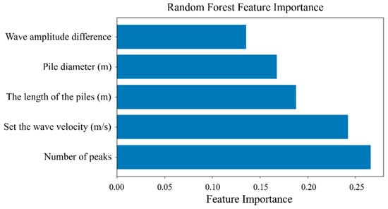
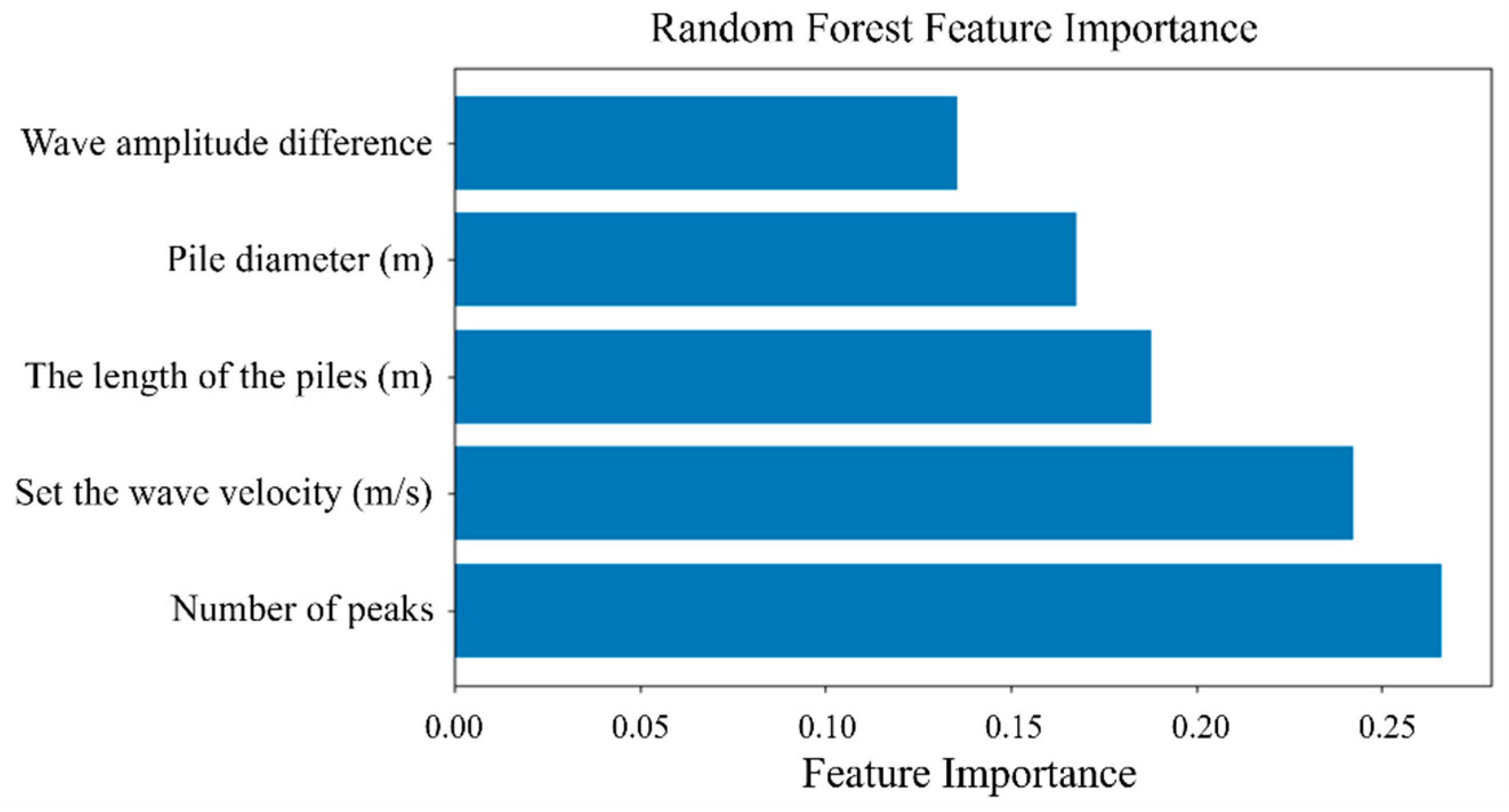
To improve model interpretability, feature importance was examined using the RF model, as shown in Figure 8. The analysis shows that the number of peaks was the most important feature for classification. This finding is physically consistent with the principles of low-strain testing, in which pile defects generate multiple reflections that increase the complexity and peak density of the reflectogram. The strong dependence of the RF model on this feature indicates that it effectively captures defect-related signal patterns. This result also supports the effectiveness of the peak count sequence in the structured modality, confirming its ability to condense complex waveform irregularities into a compact and informative indicator. However, the dominance of peak count may also introduce a potential bias in the recognition of subtle defects. Peak count is effective for identifying distinct reflection irregularities, especially for clearly defective piles. For Class II piles, however, slight or borderline defects may generate weak, broad, or partially attenuated reflections that remain below the selected amplitude thresholds. In such cases, the peak count descriptor may underestimate minor anomalies and shift these samples toward Class I or adjacent grades. Therefore, the high importance of peak count should be interpreted together with its limited sensitivity to weak reflections associated with borderline defects. The assumed wave velocity and pile length were the next most important features, as they serve as key control parameters for time to depth conversion. Their high importance reflects the need for accurate temporal scaling in order to correctly locate reflections and define defect boundaries. Pile diameter also made a meaningful contribution, which is consistent with its role in determining pile impedance and signal attenuation characteristics [32]. By contrast, waveform amplitude difference showed the lowest contribution among the selected inputs. During feature construction, alternative candidate variables, including peak amplitude, peak location, amplitude difference, pile length, pile diameter, and assumed wave velocity, were considered or included to improve robustness. Nevertheless, amplitude-related descriptors are susceptible to impact energy variation, sensor coupling conditions, pile–soil interaction, and signal attenuation under field testing conditions. Under such conditions, single point amplitude information is less stable than waveform morphology-based descriptors, which explains the relatively low contribution of waveform amplitude difference in the feature importance analysis.
Figure 8.
Feature importance of the RF model for pile integrity classification based on structured data.
Importantly, the feature importance profile also clarifies why additional feature engineering based on the present waveform records could not fully resolve the persistent difficulty in classifying Class II piles. During feature construction, several waveform descriptors were examined as candidate variables, including peak amplitude, peak location, amplitude difference, and peak count descriptors under multiple amplitude thresholds. However, amplitude-related descriptors are susceptible to impact energy variation, sensor coupling conditions, pile–soil interaction, and signal attenuation under field testing conditions. This explains why waveform amplitude difference showed the lowest contribution among the selected inputs. In comparison, the peak count sequence within the effective pile length range provides a relatively stable description of waveform irregularity, which is consistent with its dominant contribution in the RF feature importance analysis. Nevertheless, this feature strategy still has limitations for borderline defects. Class II represents a transitional state characterized by mild or borderline anomalies, in which reflection signatures are inherently weak, broad, or partially attenuated. Such reflections may remain below the selected amplitude thresholds and therefore may not develop into clearly distinguishable peak count patterns. As a result, slight defects can occupy an ambiguous region in the feature space and overlap with adjacent grades. This may partly explain the consistently lower AUC values for Class II in the ROC analysis shown in Figure 7 and the frequent misclassification into neighboring categories observed in the confusion matrices.
5.5. External Validation Using Model Pile Measurements
5.5.1. External Validation Dataset and Test Configuration
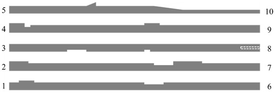
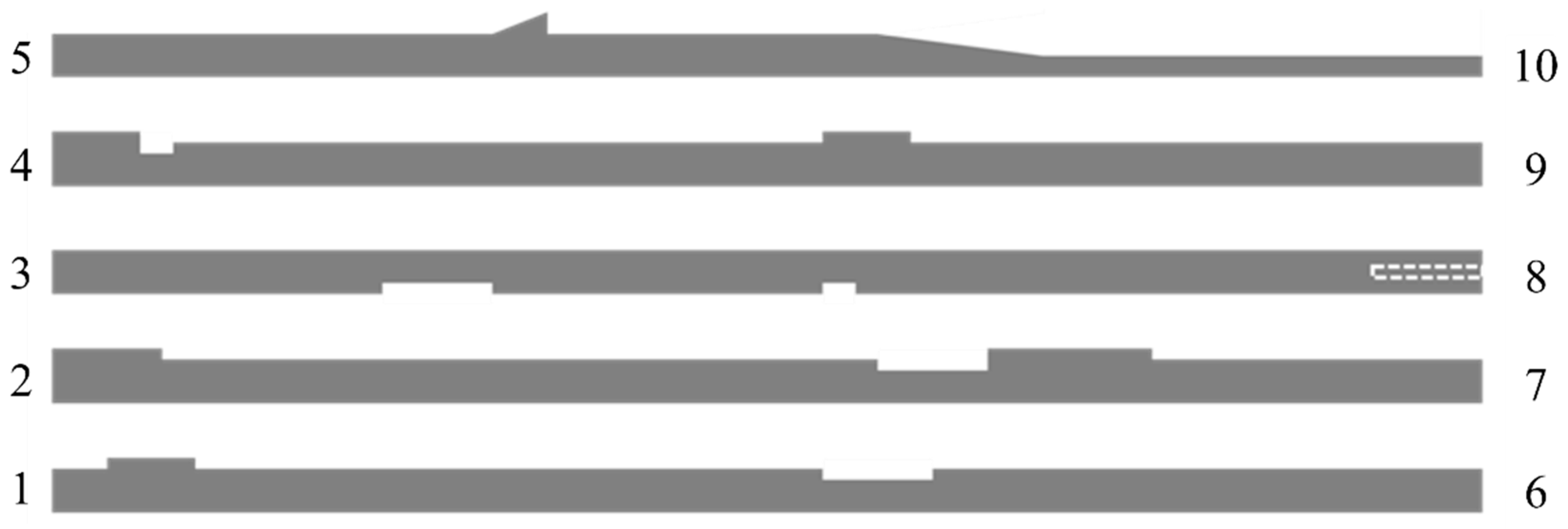
To further examine the generalization ability of the proposed models beyond the engineering dataset, a supplementary external validation test was conducted using cast model piles with designed defects. Low-strain reflection tests were performed using a PIT pile integrity tester (model C2-070; Pile Dynamics, Inc., Cleveland, OH, USA), with hammers and rods selected according to pile geometry and concrete grade. The acquired signals were processed in PIT-W20009 using standard field procedures, including filtering and exponential amplification, and were then exported for model inference. As shown in Figure 9, five precast rectangular reinforced concrete model piles made of C35 concrete were fabricated with a nominal length of 13 m and representative cross-sections of 400 mm × 400 mm, 400 mm × 500 mm, and 400 mm × 200 mm. In Figure 9, the numbers on the left and right sides denote the reflectogram record IDs obtained by testing each physical pile from opposite ends, and the dashed rectangle indicates an embedded timber block defect. To simulate common integrity anomalies, intentional geometric defects, including necking and bulging, were introduced at different locations along the pile axis. Because the defects were arranged asymmetrically, the reflectograms measured from opposite ends showed different reflection timing and attenuation characteristics. Each physical pile was therefore tested from both ends, yielding a total of 10 reflectogram records. Table 3 summarizes the external validation specimens and records and links each physical pile to its two end measurements and the corresponding defect layout.
Figure 9.
Geometry and designed defect layout of the five reinforced concrete model piles used for external validation.
Table 3.
Summary of external validation specimens, measurement records, and defect layouts.
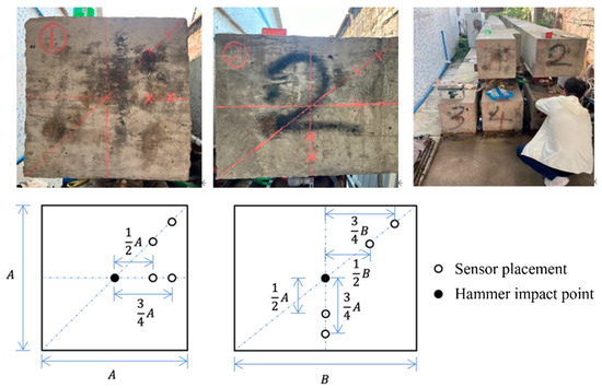
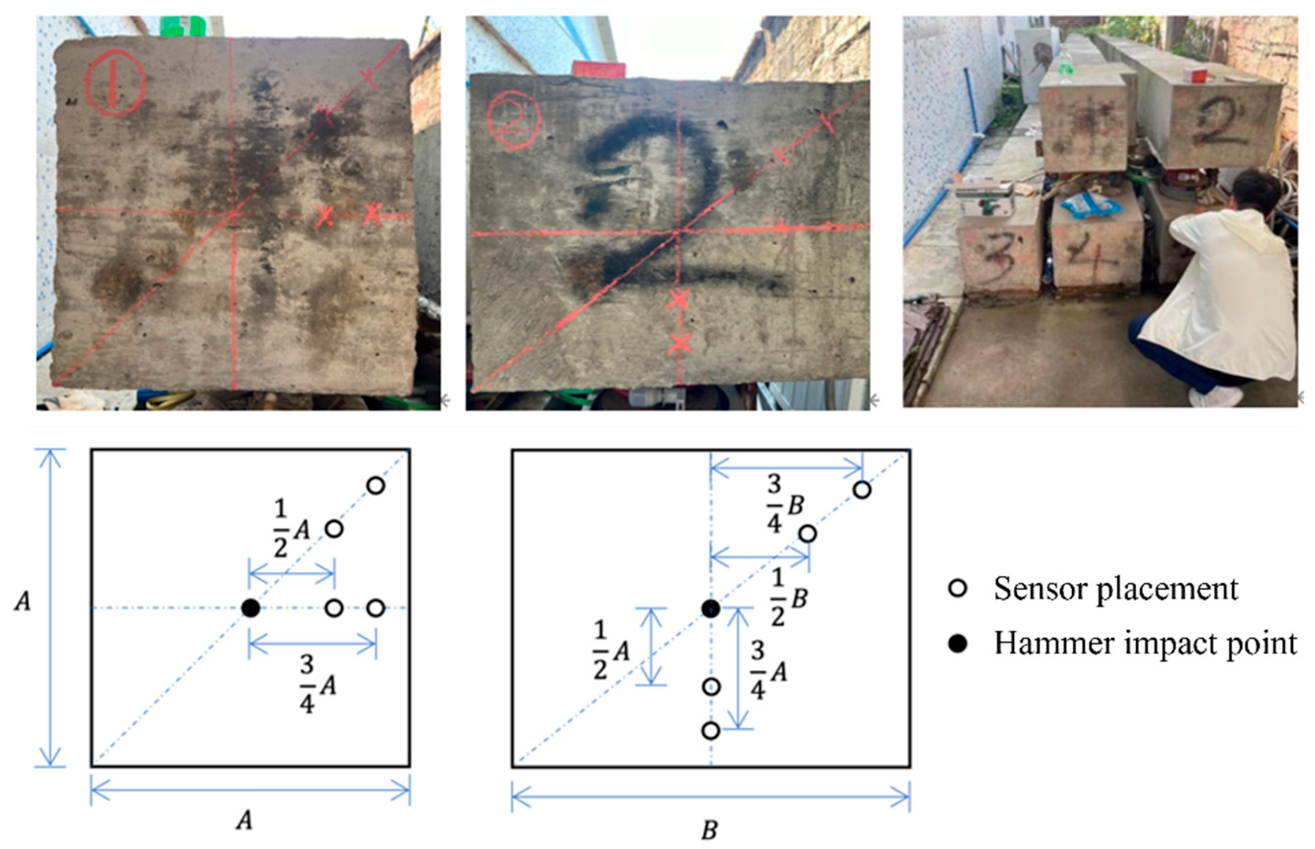
Following standard low-strain testing practice, the hammer impact was applied near the center of the pile head. As shown in Figure 10, the letters A and B denote the side dimensions of the rectangular pile head, and the fractional labels, such as 1/2A and 3/4B, indicate the relative distances used to define sensor positions. The open circles represent sensor placements, whereas the filled circle represents the hammer impact point. Sensors were mounted at multiple positions around the pile head to reduce interference from radial vibration components and to improve measurement stability for rectangular sections. Each measurement was repeated at least three times, and the representative reflectogram showing consistent excitation and clear reflection features was selected for subsequent analysis. The ground truth integrity grades for the model pile records were assigned by qualified testing engineers based on the measured reflectograms, in a manner consistent with routine inspection practice. Because the fabricated model piles were intentionally designed to represent defective conditions and therefore did not include intact Class I specimens, an additional set of 10 Class I piles from engineering practice was incorporated to complete the supplementary external validation dataset covering all four classes. These intact cases were selected based on formal inspection reports issued by qualified engineers and stable reflectograms, and they were used only for this supplementary validation. It should therefore be noted that the final external validation set combined records from two different sources, namely model pile measurements for defective cases and field measurements for intact cases. The resulting external validation set comprised 20 reflectogram records, and its class composition is summarized in Table 4.
Figure 10.
Sensor mounting positions and measurement layout at the pile head.
Table 4.
Composition of the supplementary external validation set with mixed data sources.
5.5.2. External Validation Performance
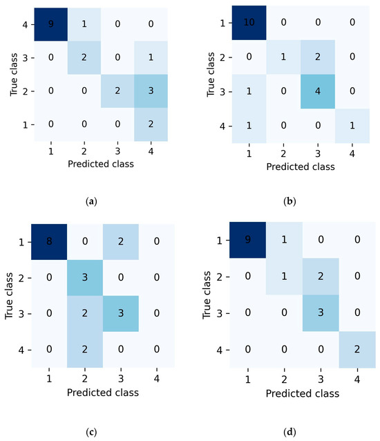
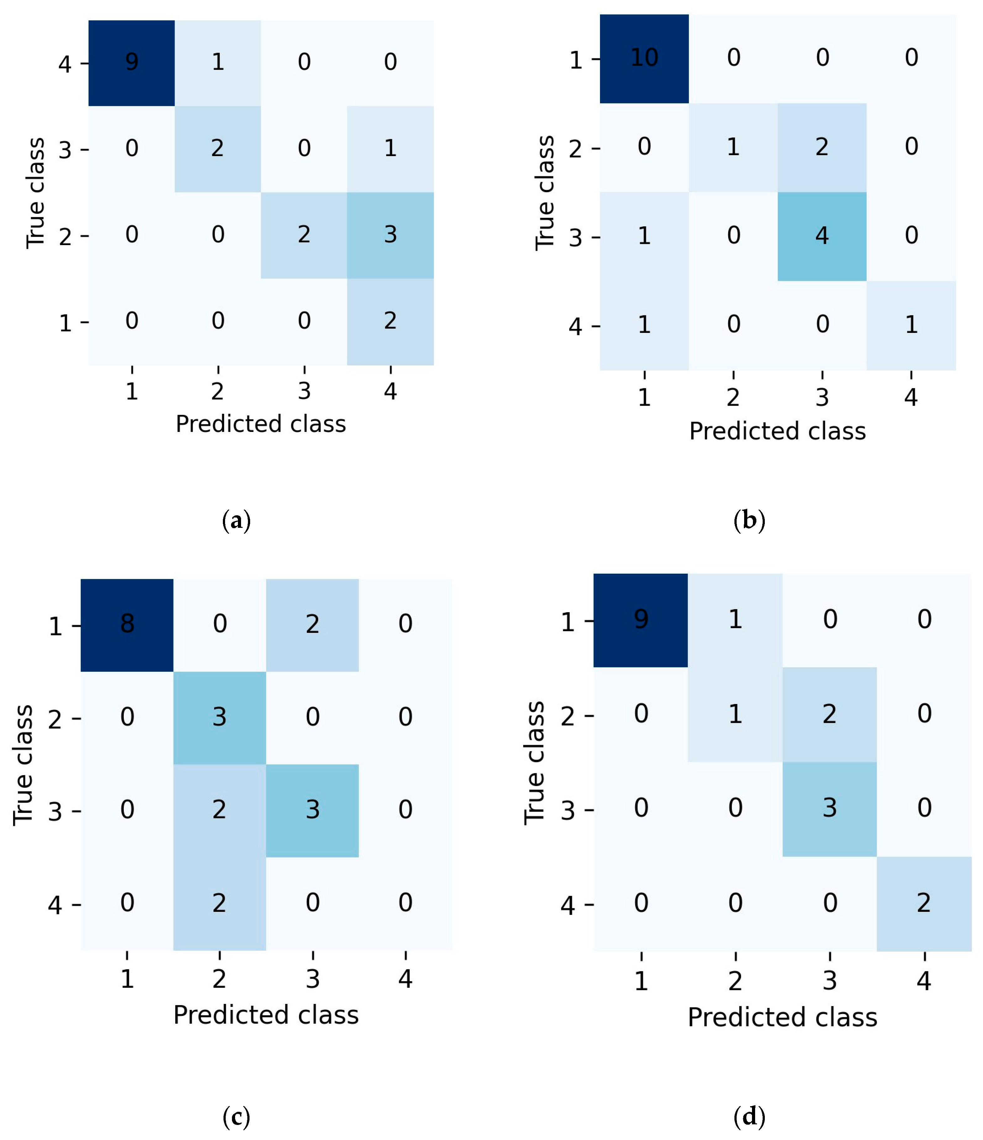
The supplementary external validation results are summarized in Figure 11 and Table 5. Overall, the four models correctly classified 15/20 samples for SVM, 16/20 for RF, 14/20 for CNN, and 17/20 for MNN, corresponding to accuracies of 75%, 80%, 70%, and 85%, respectively. Although the sample size was limited and the validation set contained records from mixed sources, the ranking of model performance remained consistent with that observed on the main evaluation subset, with the MNN showing the best overall performance. This consistency suggests that the advantage of multimodal fusion was not confined to a single training and testing split.
Figure 11.
Confusion matrices of the four models on the external validation set
: (a) SVM; (b) RF; (c) CNN; (d) MNN.
Table 5.
Overall accuracy of the four models on the supplementary external validation set.
The confusion matrices in Figure 11 further show that most of the residual errors occurred between adjacent integrity grades rather than between the intact and severely defective classes. This pattern is consistent with the results obtained on the main evaluation subset and indicates that the principal difficulty still lay in distinguishing borderline conditions with weak or overlapping reflection signatures. Compared with the single modality baselines, the MNN exhibited fewer cross-grade confusions overall, suggesting that the combination of structured and visual information improved robustness when one representation alone was insufficiently informative. However, because intact and defective samples were drawn from different sources, the present results should be interpreted as preliminary evidence of robustness across different scenarios rather than definitive proof of field generalization under balanced source conditions. The generalizability of the proposed models may also be affected by project source, pile type, soil condition, testing device, excitation condition, sensor coupling, and labeling practice. Therefore, broader validation using independent and cross-site datasets is required before the model can be considered transferable across diverse engineering conditions. Such validation is feasible in practice because routine pile integrity testing generates large numbers of low-strain records. However, it requires consistent data archiving, unified integrity labeling criteria, and standardized preprocessing procedures.
5.6. Practical Implications for Field Pile Integrity Evaluation
From an engineering application perspective, the proposed framework can be regarded as a computer-assisted decision support approach for field pile integrity evaluation. In routine low-strain testing, a large number of reflectograms are commonly generated during pile inspection, and these records are often stored as coordinate data, waveform plots, or both. Based on the preprocessing workflow established in this study, such records can be converted into paired structured descriptors and waveform images, allowing the trained model to provide preliminary integrity classification for batch screening.
The practical value of the proposed method lies mainly in improving the efficiency and consistency of preliminary interpretation. Conventional low-strain testing still depends largely on manual judgment, and interpretation may be influenced by analyst experience, signal noise, and the complexity of reflected waveforms. By applying a unified learned decision rule to both structured and image representations, the proposed multimodal framework can reduce repetitive manual workload and provide a more consistent screening reference for large-scale inspection datasets. In addition, the model output can assist engineers in identifying piles that require closer review, retesting, or verification using complementary methods. It should be emphasized, however, that the proposed framework is not intended to replace professional engineering judgment. Final integrity assessment and treatment decisions should still be made by qualified engineers based on the original testing signals, project information, site conditions, and applicable technical standards.
6. Conclusions
This study developed a dual representation multimodal learning framework for pile integrity classification into four classes using low-strain reflection testing records. By combining engineered structured descriptors with waveform images, the proposed multimodal neural network (MNN) was compared with SVM, RF, and CNN baselines. Based on the present results, the following conclusions can be drawn:
- (1)
- Among the evaluated models, the MNN achieved the best overall performance on the engineering evaluation subset, indicating that the fusion of structured descriptors and waveform images can improve overall classification robustness compared with single representation baselines.
- (2)
- The information derived from the numbers of waveform peaks identified under several amplitude thresholds proved to be informative for classification. The RF feature importance analysis showed that this information contributed strongly to the classification process, suggesting that the distribution and complexity of reflected waveform peaks within the effective pile length range provide a useful compact representation of waveform irregularity.
- (3)
- Despite the overall advantage of the MNN, all models showed limited discrimination for the borderline Class II category. This finding indicates that slight defects are intrinsically difficult to separate from adjacent grades using the current signal representations and feature set. Future work should therefore focus on introducing more defect-sensitive descriptors and physically informed signal representations.
- (4)
- Supplementary external validation using model pile records and additional intact field piles showed a consistent ranking of model performance, with the MNN remaining as the best performing model overall. However, because this validation set was limited in size and contained samples from different sources, the observed generalization should be interpreted with caution. A larger external dataset with balanced data sources is still needed before broader engineering generalization can be claimed.
These limitations define the next step of this research. Future work will focus on collecting independent and cross-site low-strain testing datasets from different projects, pile types, ground conditions, and testing devices to further evaluate the transferability and practical generalization of the proposed framework. In addition, consistent data archiving, unified integrity labeling criteria, and standardized preprocessing procedures will be required to support reliable cross-site validation.
Author Contributions
Q.-L.L.: Methodology, Investigation, Formal analysis, Validation, Writing—original draft; C.C.: Conceptualization, Writing—review and editing; M.-C.L.: Formal analysis, Methodology, Writing—review and editing; G.-L.F.: Writing—review and editing, Formal analysis; G.-X.T.: Formal analysis. All authors have read and agreed to the published version of the manuscript.
Funding
This work was financially supported by the Shenzhen Municipal Science and Technology Program Project (grant number JCYJ20230808105109018).
Data Availability Statement
Data will be made available on request.
Conflicts of Interest
The authors declare that they have no known competing financial interests or personal relationships that could have appeared to influence the work reported in this paper.
Abbreviations
| AUC | Area under the curve |
| CNN | Convolutional neural network |
| LST | Low-strain reflection testing |
| ML | Machine learning |
| MNN | Multimodal neural network |
| RBF | Radial basis function |
| RF | Random forest |
| RGB | Red, green, and blue |
| ROC | Receiver operating characteristic |
| SVM | Support vector machine |
References
- Feng, Q.; Kong, Q.Z.; Song, G.B. Damage detection of concrete piles subject to typical damage types based on stress wave measurement using embedded smart aggregates transducers. Measurement 2016, 88, 345–352. [Google Scholar] [CrossRef] [Scilit]
- O’Neill, M.W.; Sarhan, H.A. Structural Resistance Factors for Drilled Shafts Considering Construction Flaws. In Current Practices and Future Trends in Deep Foundations; American Society of Civil Engineers: Reston, VA, USA, 2004; pp. 166–185. [Google Scholar]
- Iovino, M.; Di Laora, R.; de Sanctis, L. Serviceability analysis of piled foundations supporting tall structures. Acta Geotech. 2021, 16, 3963–3973. [Google Scholar] [CrossRef] [Scilit]
- Oluwatuyi, O.E.; Ng, K.; Wulff, S.S. Improved resistance prediction and reliability for bridge pile foundation in shales through optimal site investigation plans. Reliab. Eng. Syst. Saf. 2023, 239, 109476. [Google Scholar] [CrossRef] [Scilit]
- Zhang, M.; Li, M.; Zhang, J.; Liu, L.; Li, H. Onset detection of ultrasonic signals for the testing of concrete foundation piles by coupled continuous wavelet transform and machine learning algorithms. Adv. Eng. Inform. 2020, 43, 101034. [Google Scholar] [CrossRef] [Scilit]
- Cuajao, V.C.S.; Dela Cruz, O.G.; Tabaroei, A. Comparison of static and dynamic load testing: A review. Int. J. GEOMATE 2024, 27, 119–127. [Google Scholar] [CrossRef] [Scilit]
- Sakr, M. Comparison between high strain dynamic and static load tests of helical piles in cohesive soils. Soil. Dyn. Earthq. Eng. 2013, 54, 20–30. [Google Scholar] [CrossRef] [Scilit]
- Zhang, J.; Fan, T.; Ma, H.; Li, Z. Monitoring setting and hardening of concrete by active acoustic method: Effects of water-to-cement ratio and pozzolanic materials. Constr. Build. Mater. 2015, 88, 118–125. [Google Scholar] [CrossRef] [Scilit]
- Jierula, A.; Oh, T.M.; Wang, S.; Lee, J.H.; Kim, H.; Lee, J.W. Detection of damage locations and damage steps in pile foundations using acoustic emissions with deep learning technology. Front. Struct. Civ. Eng. 2021, 15, 318–332. [Google Scholar] [CrossRef] [Scilit]
- Wan, Z.; Guo, Z.; Dai, G.; Zhou, F. Effectiveness of large-diameter combined tip-and-side post-grouted piles in deep fine sand layers: A field test study. J. Rock Mech. Geotech. Eng. 2025, in press. [Google Scholar] [CrossRef] [Scilit]
- Likins, G.E.; Rausche, F.; Miner, R.; Hussein, M.H. Verification of Deep Foundations by NDT Methods. In Design and Performance of Deep Foundations: Piles and Piers in Soil and Soft Rock; Nelson, P.P., Smith, T.D., Clukey, E.C., Eds.; Ge-otech. Spec. Publ. No. 38; ASCE: Reston, VA, USA, 1993; pp. 76–90. [Google Scholar]
- Tu, Y.; Wang, K.; Liu, X.; Rizvi, S.M.F.; Qiu, X. Wave reflection characteristics at the pile tip-soil interface under low strain dynamic condition. Comput. Geotech. 2021, 130, 103916. [Google Scholar] [CrossRef] [Scilit]
- Qiu, P.; Yang, L.; Xie, Y.; Liu, X.; Chen, Z. Pile Integrity Testing Using Non-Destructive Testing Techniques and Artificial Intelligence: A Review. Appl. Sci. 2025, 15, 8580. [Google Scholar] [CrossRef] [Scilit]
- Liu, K.H.; Zheng, J.K.; Pacheco-Torgal, F.; Zhao, X.Y. Innovative modeling framework of chloride resistance of recycled aggregate concrete using ensemble machine learning methods. Constr. Build. Mater. 2022, 337, 127613. [Google Scholar] [CrossRef] [Scilit]
- McArthur, J.J.; Shahbazi, N.; Fok, R.; Raghubar, C.; Bortoluzzi, B.; An, A. Machine learning and BIM visualization for maintenance issue classification and enhanced data collection. Adv. Eng. Inform. 2018, 38, 101–112. [Google Scholar] [CrossRef] [Scilit]
- Ahmad, A.; Chaiyasarn, K.; Farooq, F.; Ahmad, W.; Suparp, S.; Aslam, F. Compressive strength prediction via gene expression programming (GEP) and artificial neural network (ANN) for concrete containing RCA. Buildings 2021, 11, 324. [Google Scholar] [CrossRef] [Scilit]
- Gao, Y.; Li, Z.; Li, Y.; Zhu, Z.; Zhu, J. Development of chemistry-informed interpretable model for predicting compressive strength of recycled aggregate concrete containing supplementary cementitious materials. J. Clean. Prod. 2023, 425, 138733. [Google Scholar] [CrossRef] [Scilit]
- Feng, J.; Zhang, H.; Gao, K.; Liao, Y.; Gao, W.; Wu, G. Efficient creep prediction of recycled aggregate concrete via machine learning algorithms. Constr. Build. Mater. 2022, 360, 129497. [Google Scholar] [CrossRef] [Scilit]
- Protopapadakis, E.; Schauer, M.; Pierri, E.; Doulamis, A.D.; Stavroulakis, G.E.; Böhrnsen, J.U.; Langer, S. A genetically optimized neural classifier applied to numerical pile integrity tests considering concrete piles. Comput. Struct. 2016, 162, 68–79. [Google Scholar] [CrossRef] [Scilit]
- Cui, D.M.; Yan, W.; Wang, X.Q.; Lu, L.M. Towards Intelligent Interpretation of Low Strain Pile Integrity Testing Results Using Machine Learning Techniques. Sensors 2017, 17, 2443. [Google Scholar] [CrossRef] [Scilit]
- Wang, H.; Zhang, S.; Li, J.; Yuan, Y.; Zhang, F. Classification of Low-Strain Foundation Pile Testing Signal Using Recurrent Neural Network. Buildings 2023, 13, 1228. [Google Scholar] [CrossRef] [Scilit]
- Wu, C.S.; Zhang, J.Q.; Qi, L.L.; Zhuo, D.B. Defect Identification of Concrete Piles Based on Numerical Simulation and Convolutional Neural Network. Buildings 2022, 12, 664. [Google Scholar] [CrossRef] [Scilit]
- Liu, W.; Tian, S.; Hu, L. Classification of pile foundation integrity based on convolutional neural network. Arab. J. Geosci. 2022, 15, 793–800. [Google Scholar] [CrossRef] [Scilit]
- Wu, C.S.; Ge, M.; Qi, L.L.; Zhuo, D.B.; Zhang, J.Q.; Hao, T.Q.; Peng, Y.X. Multi-Defect Identification of Concrete Piles Based on Low Strain Integrity Test and Two-Channel Convolutional Neural Network. Appl. Sci. 2023, 13, 3530. [Google Scholar] [CrossRef] [Scilit]
- Kingma, D.P.; Ba, J. Adam: A Method for Stochastic Optimization. In Proceedings of the International Conference on Learning Representations (ICLR), San Diego, CA, USA, 7–9 May 2015; pp. 1–13. [Google Scholar]
- Abadi, M.; Barham, P.; Chen, J.; Chen, Z.; Davis, A.; Dean, J.; Devin, M.; Ghemawat, S.; Irving, G.; Isard, M.; et al. TensorFlow: A System for Large-Scale Machine Learning. In Proceedings of the 12th USENIX Symposium on Operating Systems Design and Implementation (OSDI 16); USENIX Association: Savannah, GA, USA, 2016; pp. 265–283. [Google Scholar]
- Huang, Z.; Guo, Y.; Huang, S.; Zhao, M. A Lightweight LLM-Based Semantic–Spatial Inference Framework for Fine-Grained Urban POI Analysis. Smart Cities 2026, 9, 13. [Google Scholar] [CrossRef] [Scilit]
- Nazir, R.B.; Hussein, O.E. Assessment of low strain wave attenuation for piles cast in very dense granular soil. In Proceedings of the 2nd International Conference on Geotechnique, Construction Materials and Environment (GEOMATE 2012), Kuala Lumpur, Malaysia, 14–16 November 2012; pp. 303–307. [Google Scholar]
- Geirhos, R.; Rubisch, P.; Michaelis, C.; Bethge, M.; Wichmann, F.A.; Brendel, W. ImageNet-trained CNNs are biased towards texture; increasing shape bias improves accuracy and robustness. arXiv 2019. [Google Scholar] [CrossRef] [Scilit]
- Shorten, C.; Khoshgoftaar, T.M. A survey on Image Data Augmentation for Deep Learning. J. Big Data 2019, 6, 60. [Google Scholar] [CrossRef] [Scilit]
- Chou, J.S.; Pham, A.D. Enhanced artificial intelligence for ensemble approach to predicting high performance concrete compressive strength. Constr. Build. Mater. 2013, 49, 554–563. [Google Scholar] [CrossRef] [Scilit]
- ASTM D5882-16; Standard Test Method for Low Strain Impact Integrity Testing of Deep Foundations. ASTM International: West Conshohocken, PA, USA, 2016.

Disclaimer/Publisher’s Note: The statements, opinions and data contained in all publications are solely those of the individual author(s) and contributor(s) and not of MDPI and/or the editor(s). MDPI and/or the editor(s) disclaim responsibility for any injury to people or property resulting from any ideas, methods, instructions or products referred to in the content. |
© 2026 by the authors. Licensee MDPI, Basel, Switzerland. This article is an open access article distributed under the terms and conditions of the Creative Commons Attribution (CC BY) license.