Prediction of the Ultimate Load-Carrying Capacity of Aluminium Alloy Columns Based on Multi-Objective Particle Swarm Optimisation and Gaussian Process Regression

Abstract

As a structural material characterised by low density, high strength, excellent corrosion resistance and recyclability, aluminium alloy tubes are finding increasingly widespread application in the construction sector. However, there is currently a lack of research on the prediction of the bearing capacity of aluminium alloy square tube columns. To investigate the failure behaviour of aluminium alloy square tube columns under axial and eccentric compression, this paper first designed 10 thin-walled aluminium alloy square tube column specimens with varying lengths, cross-sectional dimensions and wall thicknesses. Axial and eccentric compression tests were conducted, and the loading process and failure modes were analysed. Building on this, a hybrid load-bearing capacity prediction model combining Multi-Objective Particle Swarm Optimisation (MOPSO) with the Gaussian process regression (GPR) algorithm was proposed. This model is capable of automatically learning and capturing 236 sets of experimental data. Subsequently, using the established prediction model, the contributions of high-sensitivity parameters and cross-sectional influence parameters to the load-bearing capacity were determined. Based on the prediction results, a correction factor for the diameter-to-thickness ratio was introduced into the eccentric compression bearing capacity formula of the Chinese code to establish an improved calculation formula. Compared with the implicit formula provided by machine learning models, the explicit formula proposed in this paper is more suitable for practical engineering design. The results show that the prediction results agree well with the experimental results and can accurately predict the ultimate bearing capacity of aluminium alloy square columns. Compared with the bearing capacity calculation methods in existing codes, the proposed formula reduces the root mean square error (RMSE), mean absolute error (MAE) and coefficient of determination (R²) of the dataset by 70.91%, 70.85% and 64.27%, respectively, whilst increasing the coefficient of determination (R²) from 0.8107 to 0.9830 (a relative improvement of 21.25%).

1. Introduction

As the global construction industry moves towards lighter, higher-performance and more sustainable solutions, aluminium alloys—which are low in density (approximately one-third that of steel), high in strength, highly corrosion resistant and recyclable—have found widespread application in fields such as large-span spatial structures, bridge engineering, high-rise building curtain walls and marine engineering [1,2,3]. In particular, the use of aluminium alloy structural components is growing rapidly in China, Europe and North America and has become an important complement to traditional steel and concrete structures [4,5]. However, the unique physical and mechanical properties of aluminium alloys—including a lower modulus of elasticity, a stress–strain relationship lacking a distinct yield plateau, a significant strain-hardening effect, and sensitivity to initial geometric defects and residual stresses—make predicting their load-bearing capacity more complex than for steel structures [6,7]. Comparable challenges in predicting the stability and load-bearing behaviour of thin-walled metallic members have been documented for other advanced alloys. For example, experimental and numerical investigations on QN1803 high-strength stainless steel I-girders revealed that lateral–torsional buckling resistances are poorly estimated by AS 4100, EN 1993–1–1, and AISC 360–22 owing to the omission of strain-hardening effects [8]. Similarly, Wang et al. [9] reported that existing standards significantly underestimate the patch loading resistance of perforated S32001 high-strength stainless steel girders, as they fail to account for the distinct material nonlinearity and stress redistribution induced by web openings.

Aluminium alloy square tube columns are currently widely used in structural engineering. In order to accurately investigate the load-bearing capacity of aluminium alloy square tube columns, researchers have employed experimental or numerical simulation methods. A systematic experimental study was conducted by Li et al. [10] on the local buckling of 6061-T6 aluminium alloy round tubes (CHSs). A study was conducted by Rong et al. [11] on the eccentric compression behaviour of round tubes made from 7A04-T6 high-strength aluminium alloy (yield strength 540 MPa), involving stability tests on 16 test specimens and parametric analysis of 315 finite element models. Through eccentric compression tests and finite element analyses of 30 thin-walled columns made of 6082-T6 aluminium alloy, Zhao et al. [12] developed a detailed numerical model incorporating geometric and material nonlinearities. Research interest in square columns extends beyond monolithic aluminium alloy members to hybrid and composite configurations. He et al. [13] conducted axial compression tests on square double-skin hybrid concrete bar columns incorporating small-diameter concrete-infilled GFRP tubes, demonstrating that the proposed system achieves up to 79.6% higher ultimate capacity and 328.3% greater ductility than conventional double-skin columns. Furthermore, Zhang et al. [14] evaluated the seismic performance of single-plane trussed concrete-filled square steel tubular composite column frames, showing that such systems exhibit substantially improved lateral resistance, stiffness, and cumulative energy dissipation compared with conventional H-shaped steel and plain CFSST frames.

Although research into load-bearing capacity models for aluminium alloy square-tube columns has attracted considerable attention, there is little literature available on the eccentric compression of such columns. According to research by Georgantzia, E. et al. [1], current design codes fail to provide accurate strength predictions, which runs counter to the principle of cost-effective design. This is primarily because the calculation formulas are based mainly on limited experimental and numerical simulation results. Furthermore, current design codes sometimes directly apply the principles of steel structure codes, which often result in overly conservative or locally unsafe designs that do not fully account for the differences between the two materials.

In recent years, machine learning methods have demonstrated significant advantages in predicting the load-bearing capacity of structural members [15,16,17,18]. For example, Zhong et al. [19] developed an artificial neural network (ANN) model to predict the ultimate load-bearing capacity of aluminium alloy plate joints under compression–bending conditions. Machine learning methods, including LightGBM, have been applied to predict the flexural load-bearing capacity of aluminium alloy-reinforced concrete beams, with a coefficient of determination (R²) exceeding 0.93 [20].

Gaussian process regression (GPR), as a powerful Bayesian non-parametric method, has demonstrated considerable potential in the field of surrogate modelling in civil engineering [21]. Unlike traditional neural networks, GPRs are capable of providing well-calibrated estimates of prediction uncertainty and demonstrate superior performance when handling small- to medium-sized datasets with complex nonlinear relationships. In GPRs, hyperparameters are typically selected by maximising the marginal log-likelihood. However, the marginal log-likelihood function typically features a highly non-convex, multi-modal optimisation landscape, making it prone to converging to local optima and missing the globally optimal hyperparameters; it is also extremely sensitive to the structure of the kernel function, and incorrect model settings can produce misleadingly high likelihood values, leading to overfitting or underfitting. Heuristic algorithms have been widely applied in the engineering field and have demonstrated excellent results [22,23,24,25]. In particular, Multi-Objective Particle Swarm Optimisation (MOPSO) has demonstrated good performance in solving complex engineering optimisation problems involving conflicting objectives.

To address the scarcity of eccentric compression test data for aluminium alloy square (SHS) columns in the existing literature and to provide an independent experimental benchmark for validating the proposed model, this study designed and tested 10 thin-walled aluminium alloy SHS columns under axial and eccentric compression. These 10 specimens serve primarily as an external validation set to assess the generalisation capability of the MOPSO-GPR model trained exclusively on 236 literature datasets. Meanwhile, they supplement the limited SHS eccentric compression data in the open literature and provide experimental evidence for validating the proposed correction factor against the Chinese code.

Consequently, this paper designed and conducted tests on aluminium alloy square tube columns subjected to axial and eccentric compression, analysing the effects of the specimen’s cross-sectional side length, height, wall thickness, and load eccentricity on the load-bearing capacity of the columns. On this basis, the GPR algorithm was selected to establish a limit strength model for aluminium alloy square tube columns, and the MOPSO algorithm was employed to optimise the parameters of the GPR algorithm. Consequently, explicit formulas meeting the design requirements for aluminium alloy square tube columns in actual production engineering are provided. In this paper, we propose a load-bearing capacity prediction model for aluminium alloy square tube columns. By considering different compression conditions and employing a hybrid MOPSO-GPR algorithm, we elucidate the underlying patterns in the experimental data and derive explicit formulas. The remaining content of this paper is as follows.

Section 2 outlines the principles of the MOPSO algorithm, the GPR algorithm, the MOPSO-GPR algorithm, the BP algorithm, the KNN algorithm and the Random Forest algorithm. Section 3 describes the dataset used to develop the models. Section 4 presents the results and validation of both the traditional models and the proposed predictive models. Section 5 presents the correction formula based on the MOPSO-GPR algorithm and compares its computational accuracy with that of the traditional standard formula. The conclusions are presented in Section 6.

2. MOPSO-GPR

2.1. Multi-Objective Particle Swarm Optimisation (MOPSO)

The particle swarm optimisation algorithm is a bio-inspired optimisation algorithm inspired by the foraging behaviour of birds [26,27] used to solve optimisation problems. The Multi-Objective Particle Swarm Optimisation (MOPSO) algorithm builds upon the particle swarm algorithm and, within the framework of swarm intelligence, maintains a set of mutually trade-offed optimal solutions through non-dominance sorting. It balances convergence and diversity to approximate the true Pareto front. The main steps of the MOPSO algorithm are as follows:

(1)

Initialise the population and the external file. Generate N particles at random, each containing a position ${\mathrm{x}}_{\mathrm{i}}$ and a velocity ${\mathrm{v}}_{\mathrm{i}}$. Store the non-dominant solutions from the initial population in the external file to serve as an approximation of the Pareto front currently found.

(2)

Individual best (pBest) update. For each particle, its current position is compared with its historical best position pBest_i; if the current solution dominates pBest_i, pBest_i is replaced; if there is no dominance, a selection is made either randomly or based on crowding distance.

(3)

Global best (gBest) selection. Select the gBest guide particle from the external archive as the priority choice, thereby selecting a solution with a large crowding distance (sparse region), preventing particles from clustering in local regions, and maintaining the diversity of the Pareto front.

(4)

Speed and position updates. Using the classic PSO formula:

$$\begin{gathered} {\mathrm{v}}_{\mathrm{i}}(\mathrm{t}+1)=\mathsf{\omega }\cdot {\mathrm{v}}_{\mathrm{i}}\left(\mathrm{t}\right)+{\mathrm{c}}_1{\mathrm{r}}_1(\mathrm{p}\mathrm{B}\mathrm{e}\mathrm{s}{\mathrm{t}}_{\mathrm{i}}-{\mathrm{x}}_{\mathrm{i}})+{\mathrm{c}}_2{\mathrm{r}}_2(\mathrm{g}\mathrm{B}\mathrm{e}\mathrm{s}\mathrm{t}-{\mathrm{x}}_{\mathrm{i}}){\mathrm{x}}_{\mathrm{i}}(\mathrm{t}+1) \\ ={\mathrm{x}}_{\mathrm{i}}\left(\mathrm{t}\right)+{\mathrm{v}}_{\mathrm{i}}(\mathrm{t}+1) \end{gathered}$$

(1)

where $\mathsf{\omega }$ is the inertial weight, ${\mathrm{c}}_1$ and ${\mathrm{c}}_2$ are learning factors, and r₁ and r₂ are random numbers.

(5)

Determine whether the MOPSO algorithm has terminated. The algorithm stops when the maximum number of iterations is reached or the convergence criterion is satisfied; the solution set in the external file then represents the final approximate Pareto front.

2.2. Gaussian Process Regression Algorithm (GPR)

The fundamental idea behind Gaussian process regression is to learn the mapping relationship between the independent and dependent variables in a dataset and to use this mapping to predict the corresponding values of a new independent variable x* and a new dependent variable y*. To achieve this, the following covariance matrix is constructed:

$$\mathrm{K}=\left[\begin{array}{ccc}\begin{array}{cc}\mathrm{K}\left({\mathrm{x}}_1,{\mathrm{x}}_1\right)& \mathrm{K}\left({\mathrm{x}}_1,{\mathrm{x}}_2\right)\end{array}& \dots & \mathrm{K}\left({\mathrm{x}}_1,{\mathrm{x}}_{\mathrm{n}}\right)\\ \begin{array}{cc}\mathrm{K}\left({\mathrm{x}}_2,{\mathrm{x}}_1\right)& \mathrm{K}\left({\mathrm{x}}_2,{\mathrm{x}}_2\right)\end{array}& \text{…}& \mathrm{K}\left({\mathrm{x}}_2,{\mathrm{x}}_{\mathrm{n}}\right)\\ \begin{array}{cc}\begin{array}{c}\text{⋮}\\ \mathrm{K}\left({\mathrm{x}}_{\mathrm{n}},{\mathrm{x}}_1\right)\end{array}& \begin{array}{c}\text{⋮}\\ \mathrm{K}\left({\mathrm{x}}_{\mathrm{n}},{\mathrm{x}}_2\right)\end{array}\end{array}& \begin{array}{c}\text{⋱}\\ \text{…}\end{array}& \begin{array}{c}\text{⋮}\\ \mathrm{K}\left({\mathrm{x}}_{\mathrm{n}},{\mathrm{x}}_{\mathrm{n}}\right)\end{array}\end{array}\right]$$

(2)

$$\mathrm{K}\left({\mathrm{x}}_{*}, \mathrm{x}\right)=\left[\mathrm{K}\left({\mathrm{x}}_{*},{ \mathrm{x}}_1\right),\text{…}\mathrm{K}\left({\mathrm{x}}_{*},{ \mathrm{x}}_{\mathrm{n}}\right)\right]$$

(3)

$$\mathrm{K}\left(\mathrm{x},{ \mathrm{x}}_{*}\right)=\left[\mathrm{K}\left({\mathrm{x}}_1, \mathrm{x}\right),\text{…}\mathrm{K}\left({\mathrm{x}}_{\mathrm{n}}, \mathrm{x}\right)\right]$$

(4)

$${\mathrm{K}}_{**}=\mathrm{K}\left({\mathrm{x}}_{*}, {\mathrm{x}}_{*}\right)$$

(5)

In a Gaussian process regression model, each sample y can be expressed as:

$$\mathrm{y} = \mathrm{f}\left(\mathrm{x}\right) + \mathsf{\epsilon }$$

(6)

where $\mathsf{\epsilon }\text{~}\mathrm{n}0\text{’} {\mathsf{\sigma }}_{\mathsf{\epsilon }}2$. The hyperparameters in the kernel function control the specific shape of the latent function, such as whether the function changes rapidly or remains relatively stable [28].

Covariance kernel functions incorporate assumptions about the function of interest and represent the correlation between observations. Consequently, GPR modelling is essentially an inferential process aimed at determining the appropriate kernel function. The most common basic kernel functions are the squared exponential (SE), Matern class (MC) and rational quadratic (RQ) functions.

• Squared Exponential (SE)

Currently, the most commonly used kernel function is the squared exponential kernel. The formula for the squared exponential kernel is as follows [29,30]:

$$\mathrm{K}\left(\mathrm{x},{\mathrm{x}}^{\prime }\right)={\mathsf{\sigma }}_{\mathrm{f}}^2\mathrm{e}\mathrm{x}\mathrm{p}\left[-{\displaystyle \frac{1}{2}}{\displaystyle \sum _{\mathrm{i}=1}^{\mathrm{D}}}{\displaystyle \frac{{\left({\mathrm{x}}_{\mathrm{i}}-{{\mathrm{x}}_{\mathrm{i}}}^{\prime }\right)}^2}{{\mathrm{l}}_{\mathrm{i}}^2}}\right]$$

(7)

2.

Matern (MC)

Matern [31] allows the differentiability of the control function to be adjusted via a smoothing parameter, thereby better accommodating processes with finite smoothness in the real world. The formula for the Matern kernel function is:

$${\mathrm{k}}_{\mathrm{v}}\left({\mathrm{x}}_{\mathrm{i}},{\mathrm{x}}_{\mathrm{j}}\right)={\displaystyle \frac{1}{\mathsf{\Gamma }\left(\mathrm{v}\right)2^{\mathrm{v}-1}}}{\left({\displaystyle \frac{\sqrt{2\mathrm{v}}\mathrm{d}\left({\mathrm{x}}_{\mathrm{i}},{\mathrm{x}}_{\mathrm{j}}\right)}{\mathcal{l}}}\right)}^{\mathrm{v}}{\mathrm{K}}_{\mathrm{v}}\left({\displaystyle \frac{\sqrt{2\mathrm{v}}\mathrm{d}\left({\mathrm{x}}_{\mathrm{i}},{\mathrm{x}}_{\mathrm{j}}\right)}{\mathcal{l}}}\right)$$

(8)

Here,$\mathrm{d}\left({\mathrm{x}}_{\mathrm{i}}, {\mathrm{x}}_{\mathrm{j}}\right)$ denote Euclidean distances, $\mathrm{l}$ is the length scale, v controls the smoothness, and ${\mathrm{K}}_{\mathrm{v}}$ is the modified Bessel function. It is used in Gaussian process regression (GPR) to define the covariance function, thereby regulating the smoothness and flexibility of the prediction function.

3.

Rational Quadratic (RQ)

In Gaussian process regression (GPR) [31], in addition to the commonly used squared-exponential kernel function, the rational quadratic kernel function is also a common form of kernel function. This kernel function can be regarded as a weighted sum of squared-exponential kernel functions with different length scales; consequently, it offers greater flexibility when handling data with multi-scale characteristics. Its mathematical expression is shown below:

$$\mathrm{K}\left(\mathrm{x},{\mathrm{x}}^{\prime }\right)={\mathsf{\sigma }}_{\mathrm{f}}^2{\left(1+{\displaystyle \frac{{\left(\mathrm{x}-{\mathrm{x}}^{\prime }\right)}^2}{2\mathsf{\alpha }{\mathsf{\sigma }}_{\mathrm{l}}^2}}\right)}^{-\mathsf{\alpha }}$$

(9)

In this context, ${\mathsf{\sigma }}_{\mathrm{f}}^2$ is the amplitude parameter of the kernel function, which determines the overall range of variation in the function’s output; ${\mathsf{\sigma }}_{\mathrm{l}}$ is the length-scale parameter, used to measure the similarity between inputs; and $\mathsf{\alpha }$ is the scaling factor, used to control the degree of mixing across different length scales. As $\mathsf{\alpha }\to \mathsf{\infty }$, the kernel function converges to a power-law kernel.

2.3. MOPSO-GPR Model Development

This study employs the Multi-Objective Particle Swarm Optimisation (MOPSO) algorithm to automatically optimise the hyperparameters of the GPR model. To ensure full reproducibility, the detailed implementation settings, convergence characteristics, and final model configuration are explicitly documented as follows.

• Step 1: Encoding and search space of hyperparameters. Each particle encodes a complete GPR hyperparameter set, including the kernel type, length scale $l$ noise variance ${\sigma }_n^2$, and kernel-specific parameters. Based on preliminary sensitivity tests and literature recommendations, the length scale $l$ and noise variance ${\sigma }_n^2$ are searched on a logarithmic scale ($10^{-3}$ to $10^3$ and $10^{-5}$ to $l$, respectively), while the RQ scaling factor $\alpha$ is searched on a linear scale ($0.1$ to $10$). The kernel type $\kappa$ is treated as a categorical variable among SE, Matern, and rational quadratic.
• Step 2: External archive and diversity maintenance. A dynamic external archive with a maximum capacity of 1000 solutions is employed to store non-dominated solutions discovered during the search. An adaptive grid strategy ($10\times 10$ grids per objective) is applied to maintain diversity. When the archive exceeds its capacity, the solution located in the most crowded grid is discarded. The global best (gBest) guide is selected from the least crowded grid to prevent premature convergence.
• Step 3: Fitness evaluation and Pareto front construction. Three conflicting objectives are simultaneously optimised: (1) prediction error $f_1=1-R_{CV}^2$ (minimised, where $R_{CV}^2$ is the 10-fold cross-validation coefficient of determination); (2) generalisation penalty $f_2={RMSE}_{val}-{RMSE}_{train}$ (minimised, to prevent overfitting); and (3) model complexity $f_3={rank}_{eff}\left(\mathrm{K}\right)/n$ (minimised, where $\mathrm{K}$ is the covariance matrix and $\mathrm{n}$ is the sample size). Non-dominated sorting is performed at each iteration to construct the Pareto front.
• Step 4: Convergence characteristics. The algorithm terminates when the maximum number of generations (50) is reached.
• Step 5: Selection of the final solution from the Pareto front. A weighted scoring method is adopted to select the final compromise solution. The composite score S is computed as:

  $$\mathrm{S}=0.60{\tilde{\mathrm{f}}}_1+0.25{\tilde{\mathrm{f}}}_2+0.15{\tilde{\mathrm{f}}}_3$$

  (10)

  where ${\tilde{f}}_i$ denotes the normalised value (min-max scaling) of the $i$-th objective. The rationale for this weighting scheme is rooted in the engineering priorities of bearing capacity prediction: (i) predictive accuracy is paramount for structural safety assessment, hence the highest weight (60%); (ii) generalisation capability ensures robust performance on unseen specimens, which is critical given the heterogeneity of the collected dataset (25%); and (iii) model complexity is penalised to mitigate overfitting, yet GPR inherently regularises through its kernel structure, warranting a lower weight (15%).
• Step 6: Final kernel configuration and model fitting. Based on the above content, this paper chooses SE as the final kernel function. The final GPR model is constructed with the following hyperparameters determined through the MOPSO optimisation and 5-fold cross-validation. The final model is trained on the full training set and evaluated on the independent test.

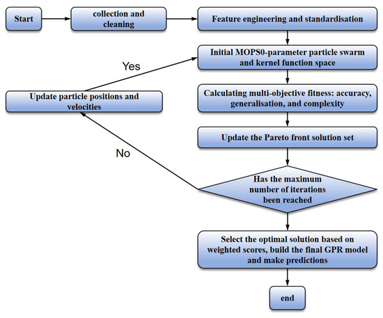
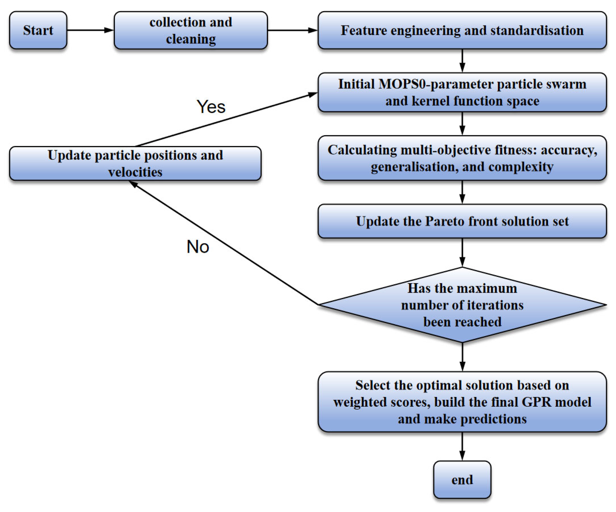
The flowchart of the MOPSO-GPR algorithm is shown in Figure 1.

Figure 1. Model construction flowchart.

3. Data Collection and Preprocessing

This chapter provides a detailed account of the sources of the experimental data, the process of constructing the dataset, and the data preprocessing methods. Through systematic data collection and a scientific preprocessing strategy, this paper provides reliable data support for model training.

3.1. Source of Test Data

3.1.1. Sample Description

The aluminium alloy square tube column specimens were fabricated from seamless material, all of which were of the 6063-T5 grade. The load-bearing capacity of the aluminium alloy square tube columns is primarily related to the cross-sectional side length B, the specimen height L, the wall thickness t of the aluminium alloy tube, and the load eccentricity e. This study investigated the compressive behaviour of 10 medium-to-long aluminium alloy square tube columns; the specimen parameters are shown in Table 1. To investigate the relevant buckling behaviour of the specimens, with the exception of specimen FZ3E0, the width-to-thickness ratios of the other specimens exceeded the limits specified in the Chinese ‘Code for Design of Aluminium Alloy Structures’ [32]. The formulae for the slenderness ratio and width-to-thickness ratio in the code are as follows:

$$\lambda = {\displaystyle \frac{L}{i_x}}$$

(11)

$${\lambda }_t={\displaystyle \frac{b}{t}}$$

(12)

Table 1. Parameters of aluminium alloy square tube column specimens.

Specimen	B/mm	L/mm	t/mm	e/mm	λt	λ
FZ1E0	100	700	3	0	31.3	17.7
FZ2E0	100	700	4	0	23.0	17.8
FZ3E0	100	700	5	0	18.0	18.0
FZ4E0	100	800	3	0	31.3	20.2
FZ5E0	100	900	3	0	31.3	20.7
FZ1E15	100	700	3	15	31.3	17.7
FZ1E30	100	700	3	30	31.3	17.7
FZ7E0	150	1050	3	0	48.0	17.5
FZ7E15	150	1050	3	15	48.0	17.5
FZ7E30	150	1050	3	30	48.0	17.5

In the equation, λ is the slenderness ratio of the member, ${\mathrm{i}}_{\mathrm{x}}$ is the radius of gyration, ${\mathsf{\lambda }}_{\mathrm{t}}$ is the width-to-thickness ratio, and b is the clear width of the plate.

3.1.2. Testing of Aluminium Alloy Properties

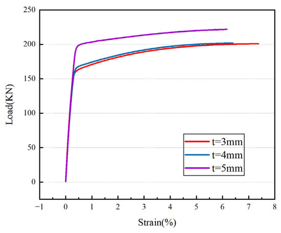
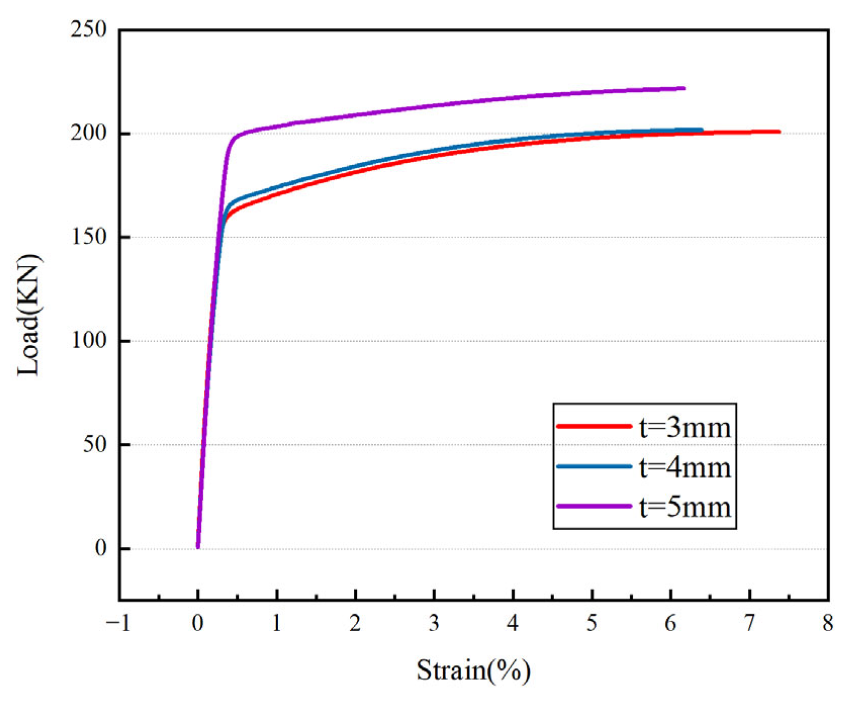
The aluminium alloy square tube columns are made from 6063-T5 aluminium alloy. In accordance with the sampling requirements of GB/T228.1-2021’ [33] Tensile testing of metallic materials: Part 1: Methods at room temperature’, testing shall be conducted at room temperatures between 10 °C and 35 °C, with tensile specimens taken from uncut aluminium alloy columns; three standard specimens were selected from each of the 3 mm, 4 mm and 5 mm thick aluminium alloy square tube columns, and the mean values were calculated using linear interpolation of the measured data. The mean results are shown in Figure 2 and Table 2, where E is the modulus of elasticity, ${\mathsf{\sigma }}_{0.05}$ and ${\mathsf{\sigma }}_{0.2}$ are the material stresses at residual strains of 0.05% and 0.2%, respectively; ${\mathsf{\sigma }}_{\mathrm{u}}$ is the ultimate stress of the material, and n is the strain hardening index.

Figure 2. Stress–strain curve.

Table 2. Test results for aluminium alloy square tube specimens.

t/mm	E/MPa	σ0.05/MPa	σ0.2/MPa	σu/MPa	n
3	72,500	155	162	201	17
4	66,800	160	167	202	17
5	66,267	192	199	222	21

3.1.3. Loading, Strain Gauge and Displacement Transducer Arrangement

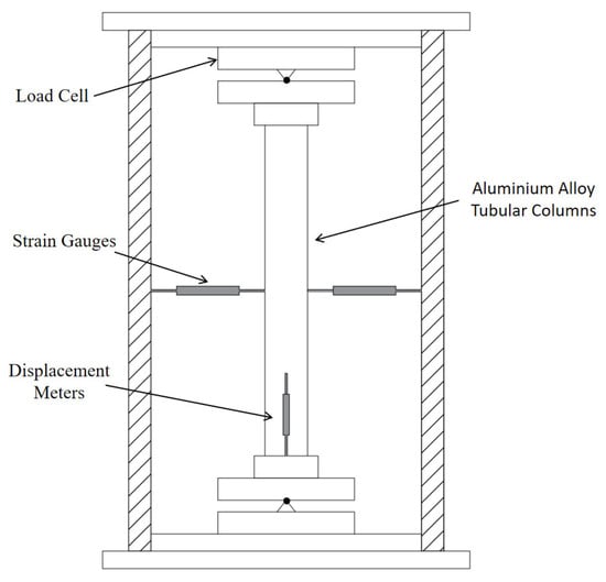
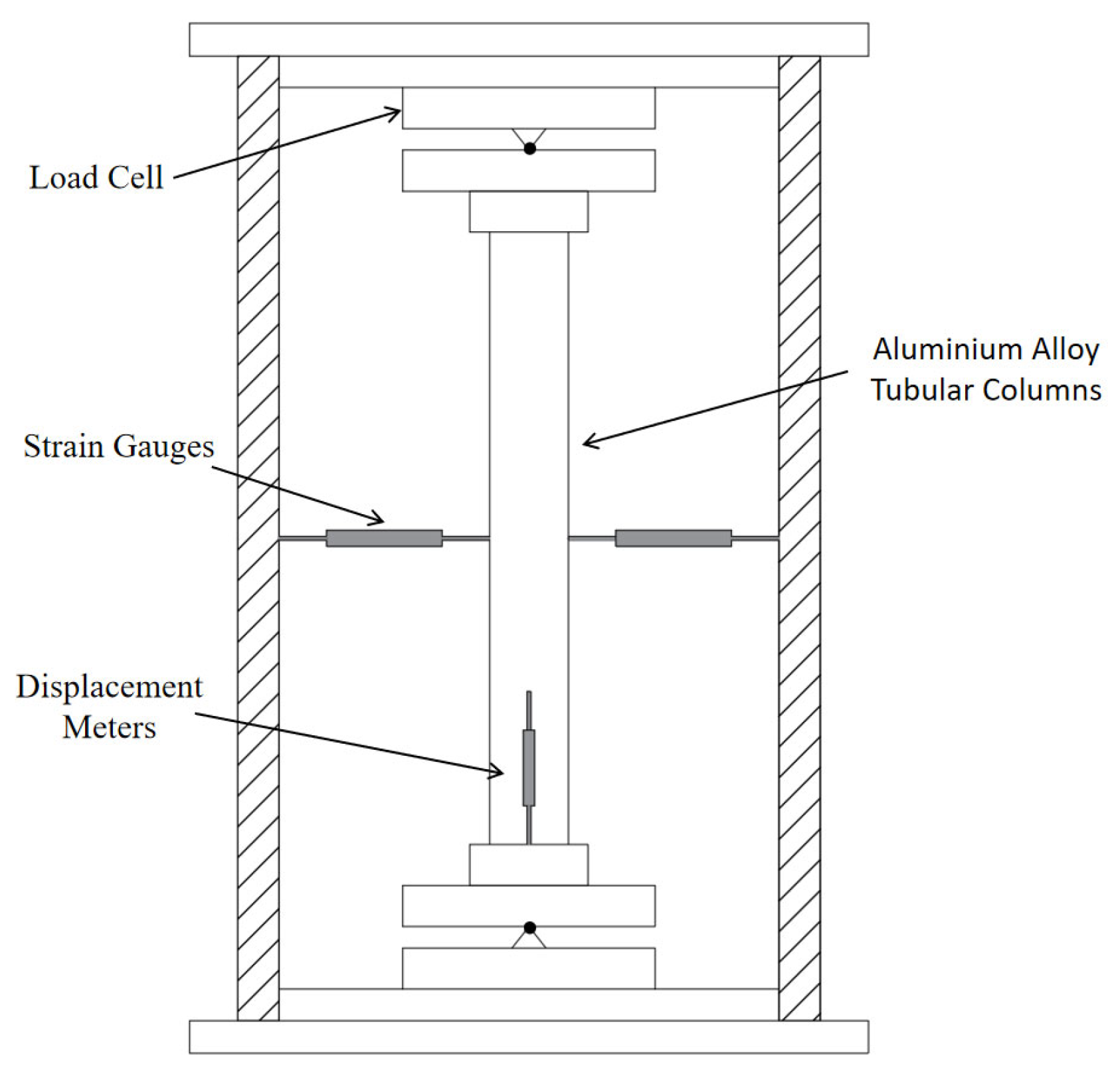
Strain gauges were installed on three cross-sections located at 1/4, 1/2, and 3/4 of the column height, with four gauges per section (12 in total). Specifically, the strain gauges at the 1/4 and 3/4 height sections were arranged along the cross-sectional axis within the bending plane. The displacement measurement system comprised the following components: two wire displacement transducers mounted on the bottom end plate to measure axial vertical displacement and two displacement transducers installed at the mid-height of the column along the cross-sectional axis in the bending plane to measure lateral horizontal displacement. As shown in Figure 3, the test setup restrained all three translational degrees of freedom at the column ends as well as the rotational degrees of freedom about the y and z axes at both ends. The test was conducted under displacement-controlled mode with a loading rate of 0.1 mm/min. The termination criterion was determined in accordance with the Specification for Seismic Test of Buildings (JGJ/T 101-2015) [34]: the specimen was deemed to have failed and the test was terminated when the load dropped below 85% of the peak load N or when significant damage occurred, rendering the specimen unsuitable for continued loading. The load level of 0.85 Nu was adopted as the failure point corresponding to the ultimate bearing capacity, providing a consistent basis for defining strength degradation and ductility performance.

Figure 3. Test instrumentation schemes.

3.1.4. Test Results

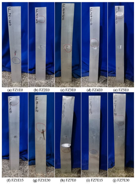
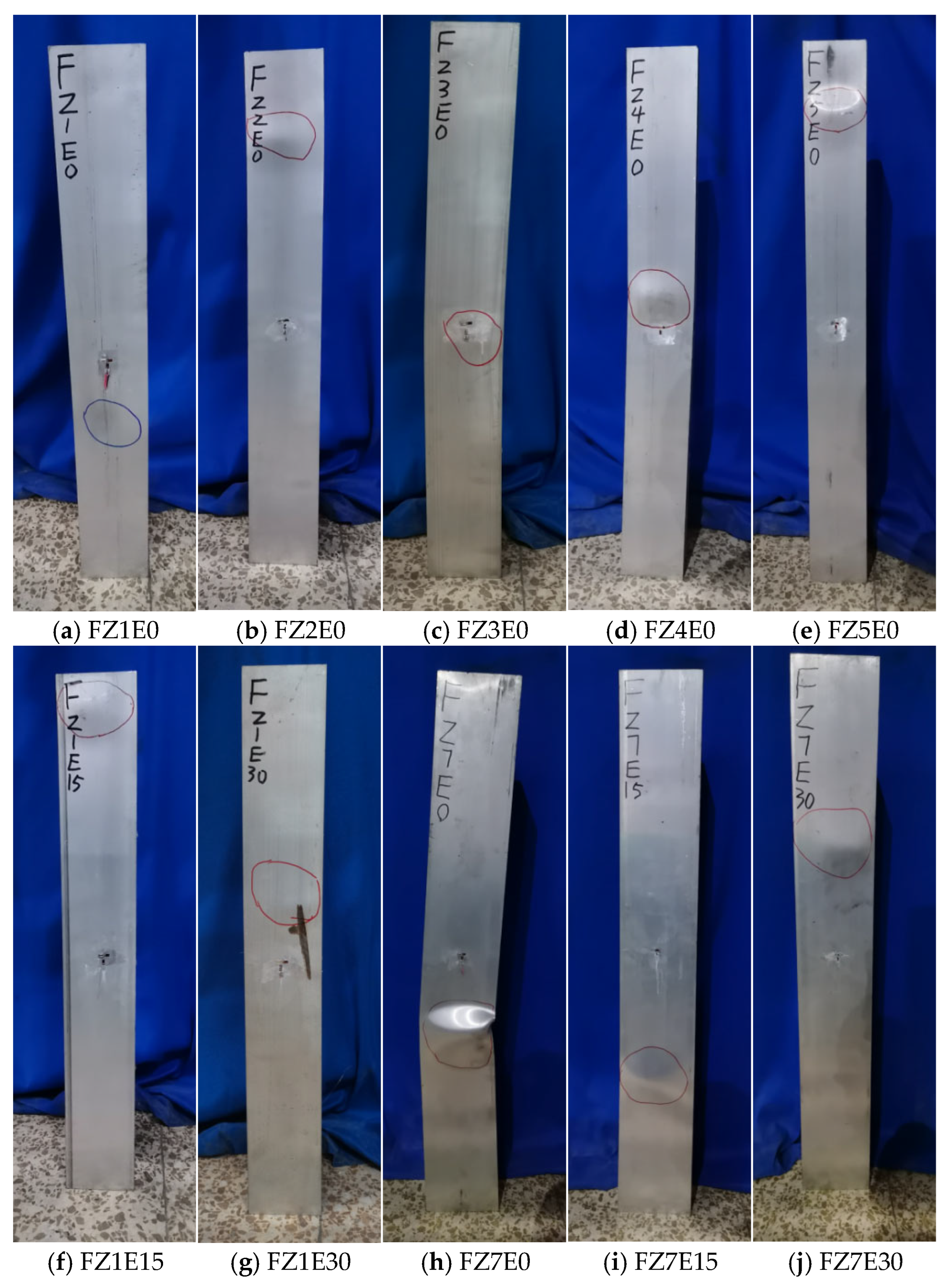
As shown in Figure 4, during loading, the specimens exhibited progressively divergent buckling behaviour as axial or eccentric compressive forces increased: with the exception of FZ7E0 and FZ1E15, all specimens exhibited global buckling, characterised by significant lateral deflection of the column body, forming single-wave or double-wave bending deformations. The deflection curves followed a sinusoidal pattern, with the column top shifting towards the compressed side; FZ7E0, however, exhibited a distinctive local crushing mode, with a pronounced local ‘barrel-shaped’ indentation and flattening of the cross-section occurring in the middle of the column height and the wall panels buckling inwards; this is characteristic of local buckling in thin-walled tubes or plastic crushing in short columns. FZ1E15 exhibited local buckling characteristics, with local bulging deformation of the tube wall, whilst the overall deflection remained small. Under eccentric loading, all specimens exhibited a unidirectional bending tendency towards the compressed side, whereas specimens under axial compression displayed symmetrical global buckling waveforms. For all specimens, the load-carrying capacity declined rapidly after reaching the peak load, and the deformation of the column body increased sharply.

Figure 4. Failure modes of aluminium alloy column specimens.

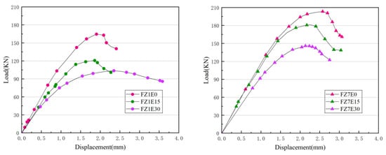
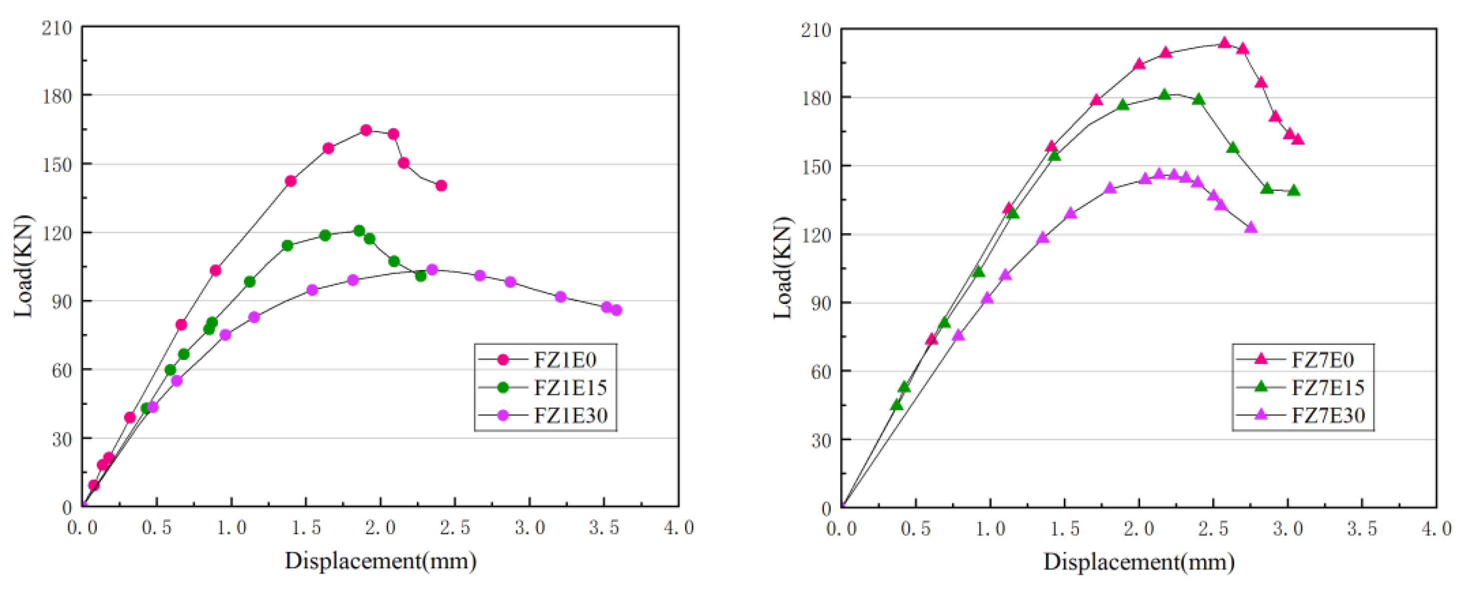
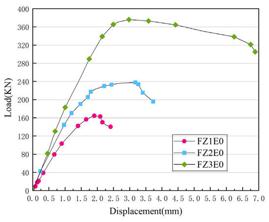
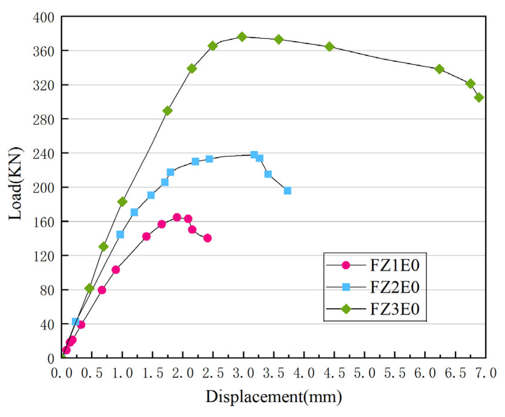
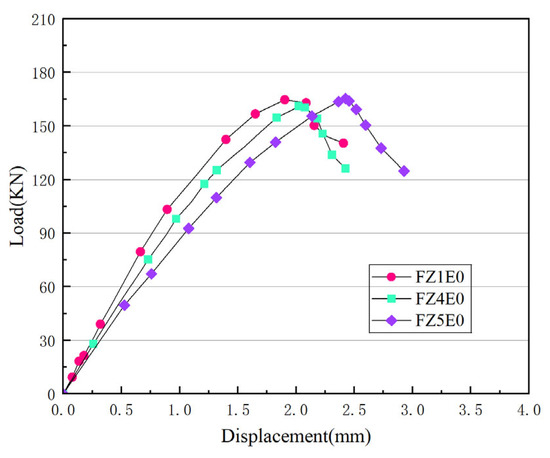
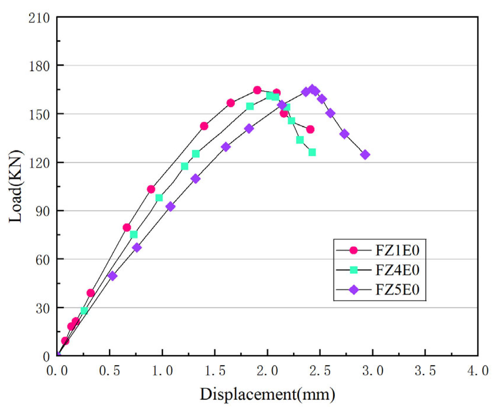
To analyse the influence of the specimen’s eccentricity, the wall thickness of the aluminium alloy square tube and the specimen height on the specimen’s load-bearing behaviour, the point at which the load drops to 0.85${\mathrm{N}}_{\mathrm{u}}$ is defined as the specimen’s failure point. The load–displacement (N-$\text{∆}$) curve for the aluminium alloy square tube column specimens is shown in Figure 5, Figure 6 and Figure 7.

Figure 5. Load-vertical displacement curves of specimens under different eccentricities.

Figure 6. Load vertical displacement curve of specimens under different wall thicknesses.

Figure 7. Load vertical displacement curve of specimens under different heights.

As shown in Figure 5, the specimens were divided into two groups based on their width-to-thickness ratio: the first group had a width-to-thickness ratio of 31.3, and the second group had a width-to-thickness ratio of 48.0. For the first group of specimens, as the eccentricity was increased sequentially from 0 to 30 mm, the ultimate load-bearing capacity of the specimens decreased by 26.7% and 37.0%, respectively; the displacement at the failure point of the specimen with an eccentricity of 15 mm showed no significant change, whereas the displacement at the failure point of the specimen with an eccentricity of 30 mm increased by 23.7%. For the second set of specimens, as the eccentricity was increased sequentially from 0 to 30 mm, the ultimate load-bearing capacity of the specimens decreased by 10.9% and 28.2%, respectively; the displacement at the point of failure showed no significant change in either case. From the above analysis, it can be seen that the load-bearing capacity of the specimens decreases significantly with an increase in eccentricity; however, as the width-to-thickness ratio of the specimens increases, the extent of the influence of changes in eccentricity on the load-bearing capacity of the specimens diminishes.

As shown in Figure 6, the third group presents the test results for specimens of aluminium alloy square tubes with varying wall thicknesses. As the wall thickness of the aluminium alloy square tubes increased from 3 mm to 5 mm, the ultimate load-bearing capacity increased by 44.5% and 128.4%, respectively; the displacement at the point of failure increased by 41.6% and 182.8%, respectively. Based on the above analysis, it can be seen that specimens with greater thickness and a smaller width-to-thickness ratio exhibit a significant increase in ultimate load-bearing capacity, demonstrating superior compressive strength; furthermore, the curves in the decline phase are flatter, indicating better ductility.

Figure 7 shows the test results for the fourth group, namely the load–vertical displacement curves for specimens of different heights. As shown in Figure 7, there is no significant variation in the ultimate load-bearing capacity or displacement at the point of failure for the specimens in the fourth group, indicating that changes in the height of the aluminium alloy columns have little effect on the axial compression stiffness and ductility of the specimens. This is because the cross-section of the specimens is S100 (side length 100 mm) with a wall thickness of 3 mm, and its width-to-thickness ratio (b/t = 100/3 ≈ 33.3) lies within the critical range. The buckling load (Euler buckling) of aluminium alloy square tube columns is inversely proportional to the square of the length. As the maximum specimen length (900 mm) has not yet reached the critical value, and the section’s moment of inertia is relatively large, the critical load for global buckling is significantly higher than that for local buckling. Consequently, under axial compression, local plate buckling is likely to occur, with the critical stress depending solely on the material properties and the width-to-thickness ratio and bearing little relation to the specimen length.

The above analysis indicates that an increase in eccentricity leads to a significant reduction in the ultimate load-bearing capacity of the test specimen. Furthermore, specimens with a smaller width-to-thickness ratio exhibit greater sensitivity under eccentric loading, with a more pronounced decrease in their ultimate load-bearing capacity. This phenomenon can be attributed to the relatively lower sectional stiffness of specimens with a smaller width-to-thickness ratio, which makes them more susceptible to additional bending moments and local buckling under eccentric loading, thereby accelerating the failure process. An increase in the wall thickness of aluminium alloy square tubes significantly enhances the specimen’s ultimate load-bearing capacity and ductility, resulting in a flatter curve and a smaller decline following the peak load. However, the effect of specimen height on load-bearing capacity and ductility is not pronounced. This is because the specimen’s aspect ratio falls within a critical range, and local buckling is likely to occur under axial compression; the critical stress depends primarily on material properties and the aspect ratio and is less influenced by specimen length.

In summary, different compression conditions have a significant impact on the load-bearing capacity of aluminium alloy columns. Compared with axial compression, eccentric compression leads to a substantial decrease in the specimen’s ultimate load-bearing capacity. For the first group of specimens (width-to-thickness ratio 31.3), the load-bearing capacity decreased by 26.7% and 37.0%, respectively, as the eccentricity increased from 0 to 30 mm; for the second group of specimens (width-to-thickness ratio 48.0), the load-bearing capacity decreased by 10.9% and 28.2%, respectively. This indicates that an increase in eccentricity significantly reduces the ultimate load-bearing capacity of the specimens and that specimens with a smaller width-to-thickness ratio are more sensitive to eccentric loading, exhibiting a greater reduction in load-bearing capacity. The mechanism lies in the fact that, under eccentric loading, the cross-section not only bears axial compression but also experiences additional bending moments, which induce premature local buckling and global bending deformation in the specimen, thereby accelerating the failure process.

Since these 10 specimens focus on two cross-sectional sizes (100 mm and 150 mm) with a single aluminium alloy grade (6063-T5), the slenderness ratio λ is confined to the intermediate range (17.5–20.7). These parameters are representative of aluminium alloy columns commonly used in curtain wall supports and light spatial structures; however, they do not encompass high-strength alloys (e.g., 7A04-T6, 6082-T6), thin-walled sections with large width-to-thickness ratios, or slender columns with high slenderness ratios. Consequently, the primary role of these tests is to provide a targeted, independent validation benchmark rather than to establish universal empirical laws. The generalisation of the proposed model to broader design scenarios is supported by the extensive database described in Section 3.2.

3.2. Database Development

In order to construct a high-quality machine learning dataset, in addition to the test data mentioned above, this study collected load-bearing capacity test data for aluminium alloy square tubes from multiple sources and carried out data standardisation and normalisation as well as sensitivity analysis.

3.2.1. Data Sources and Collection

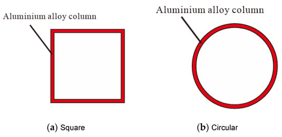
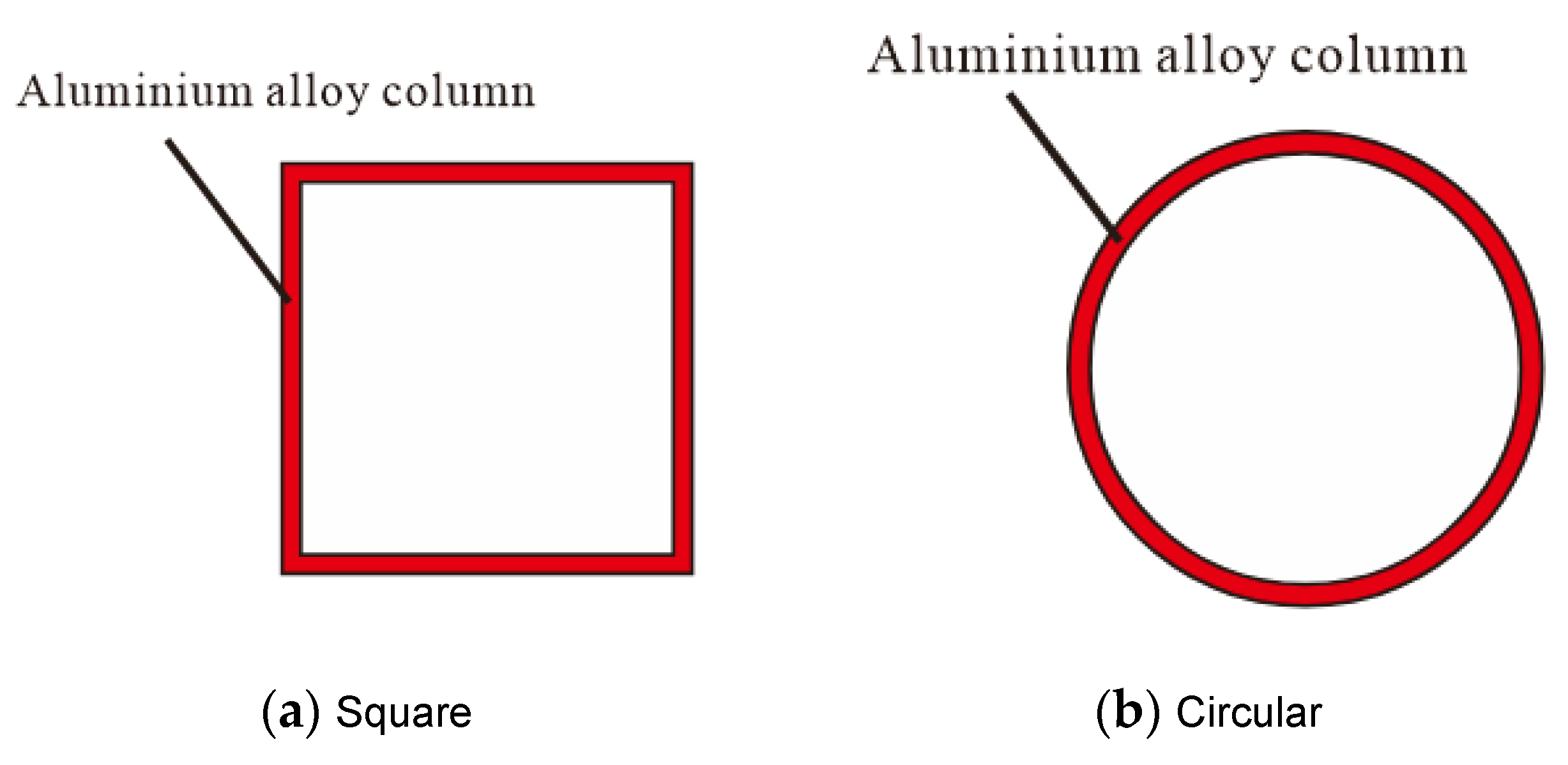
To construct a comprehensive machine-learning dataset, 236 sets of experimental data were compiled exclusively from the published literature [10,11,35,36,37,38,39,40,41,42,43,44,45,46], comprising 165 axial compression load-bearing test specimens and 81 oblique compression load-bearing test specimens, which together form the aluminium alloy columns load-bearing capacity dataset. The dataset primarily includes circular and square cross-sections, as shown in Figure 8. The tests conducted in the relevant literature all involved applying axial and oblique compression to aluminium alloy columns using a hydraulic press to obtain their load-bearing capacity data. As shown in Table 3 and Table 4, compared with the self-conducted tests, the compiled database exhibits substantially broader parametric coverage: the cross-sectional dimension D ranges from 18 mm to 203 mm, wall thickness t from 1.1 mm to 8.0 mm, member length L from 83 mm to 3490 mm, and slenderness ratio λ from 3.0 to 181.1. The dataset includes multiple aluminium alloy grades (e.g., 6061-T6, 6082-T6, 7A04-T6) and various heat treatments, thereby mitigating the material limitation of the experimental programme. The inclusion of both square hollow sections (SHSs) and circular hollow sections (CHSs) further enhances the geometric diversity. It is this extensive heterogeneity in the training data that enables the MOPSO-GPR model to learn generalised mapping relationships and ensures the proposed explicit formula is applicable beyond the narrow experimental domain.

Figure 8. Common cross-sectional shapes of aluminium alloy tubing.

Table 3. Test parameters for aluminium alloy columns.

Parameters	Unit	Minimum Value	Maximum Value	Mean	Standard Deviation
D	mm	18.0	203.0	63.7	41.5
t	mm	1.1	8.0	3.0	1.45
L	mm	83.0	3490.0	1208.1	810.2
A	mm2	197.7	2944.0	795.8	831.3
E	GPa	64.7	76.5	69.9	3.1
λ	-	3.0	181.1	64.0	52.2
e	mm	0.0	70.0	8.8	13.7
fy	MPa	64.8	510.0	242.3	87.0

Table 4. Test parameters for biased aluminium alloy columns.

Parameters	Unit	Minimum Value	Maximum Value	Mean	Standard Deviation
D	mm	50	203.0	86.9	21.2
t	mm	1.57	8	4.0	1.3
L	mm	500.0	3400.0	1679.6	789.6
A	mm2	238.9	2312.2	1075.8	392.0
E	GPa	64.7	76.5	69.3	3.8
λ	-	7.6	102.2	48.8	24.4
e	mm	4.8	51.9	20.0	10.5
fy	MPa	162	510.0	310.5	98.1

After collating the experimental data from the above literature, the following factors influencing the axial and eccentric compressive load-bearing capacities of aluminium alloy columns were identified: 1. Outer diameter D (mm), 2. Wall thickness t (mm), 3. Length L (mm), 4. Cross-sectional area A (mm²), 5. Modulus of elasticity E (GPa), 6. Slenderness ratio λ, 7. Eccentricity e (mm). Table 3 and Table 4 list the minimum, maximum, mean and standard deviation of the load-bearing capacity test data for aluminium alloy columns under different loading conditions.

Given the scarcity of eccentric compression test data for aluminium alloy SHS columns in the open literature, CHS data were incorporated to enrich the dataset and enhance model robustness. All input features ($\lambda ,D/t,A,E,e$) are fundamental physical or normalised parameters applicable to thin-walled column members regardless of cross-sectional shape. The proposed explicit formula (Equation (27)) has $D$ in the correction factor taken as the side length for square sections or the outer diameter for circular sections.

3.2.2. Data Standardisation

To minimise the impact of different units and outliers on model optimisation, this study employed two distinct normalisation strategies for the input features and the output target, respectively.

(1)

Normalisation of input features: RobustScaler handles numerical features

RobustScaler is a feature scaling method based on robust statistics [47], by standardising the data using the median and the interquartile range (IQR), rather than the mean and standard deviation used in traditional standardisation methods. The transformation formula for this method is:

$${\mathrm{x}}^{*}={\displaystyle \frac{\mathrm{x}-\mathrm{m}\mathrm{e}\mathrm{d}\mathrm{i}\mathrm{a}\mathrm{n}\left(\mathrm{x}\right)}{\mathrm{I}\mathrm{Q}\mathrm{R}\left(\mathrm{x}\right)}}$$

(13)

The IQR (Interquartile Range) refers to the interquartile range of the sample.

The reasons for selecting this method are as follows:

• Certain geometric parameters in the dataset are skewed or contain a small number of outliers.
• Compared to StandardScaler, RobustScaler is less sensitive to outliers and ensures the robustness of the scaling process.
• It helps improve the approximation capability of the Gaussian process regression model in highly skewed sample intervals.

(2)

Normalisation of the output variable (the target for bearing capacity prediction): StandardScaler normalisation

StandardScaler is a feature scaling method based on statistical parameters [48], which transforms data into a standard normal distribution by subtracting the mean and dividing by the standard deviation. The transformation formula for this method is:

$${\mathrm{y}}^{*}={\displaystyle \frac{\mathrm{y}-\mathsf{\mu }}{\mathsf{\sigma }}}$$

(14)

Compared to input features, output values are more suitable for StandardScaler for the following reasons:

• In Gaussian process regression (GPR), the likelihood assumes that the output follows a Gaussian distribution; mean-variance standardisation is more consistent with the mathematical structure of the GP.
• It helps to accelerate the convergence of the optimisation process for kernel hyperparameters (length-scale, noise level).
• It ensures that the loss function (RMSE) remains on the same order of magnitude across different folds of cross-validation, thereby enhancing the stability of MOPSO multi-objective optimisation.

During the denormalisation stage, the same mean and standard deviation are used to restore the data to their original units, thereby ensuring the interpretability of the results.

3.3. Sensitivity Analysis

To determine the effect of influencing factors on the load-bearing capacity, a sensitivity analysis of these parameters is required. By analysing the sensitivity of these parameters, we can simplify the model by reducing the number of parameters, thereby increasing the speed of the calculations. Currently, the cosine magnitude method [49,50] is commonly used to analyse the radial sensitivity of influencing factors. Consequently, this paper also employs the relationship strength formula from the cosine magnitude method to calculate the sensitivity values of each influencing factor. The relationship strength formula is as follows:

$$\mathrm{r}={\displaystyle \frac{{\displaystyle {\sum }_{\mathrm{k}=1}^{\mathrm{n}}}{\mathrm{x}}_{\mathrm{i}\mathrm{k}}{\mathrm{y}}_{1\mathrm{k}}}{\sqrt{{\displaystyle {\sum }_{\mathrm{k}=1}^{\mathrm{n}}}{\mathrm{x}}_{\mathrm{i}\mathrm{k}}^2{\displaystyle {\sum }_{\mathrm{k}=1}^{\mathrm{n}}}{\mathrm{y}}_{1\mathrm{k}}}}}={\displaystyle \frac{{\mathsf{\sigma }}_{\mathrm{x}\mathrm{y}}}{{\mathsf{\sigma }}_{\mathrm{x}}{\mathsf{\sigma }}_{\mathrm{y}}}}$$

(15)

In Equation (15), $\left({\mathrm{x}}_{\mathrm{ik}} = \left[\begin{array}{cccc}{\mathrm{x}}_{\mathrm{i}1}& {\mathrm{x}}_{\mathrm{i}2}& \text{⋯}& {\mathrm{x}}_{\mathrm{in}}\end{array}\right]\right), \left({\mathrm{y}}_{1\mathrm{k}}= \left[\begin{array}{cccc}{\mathrm{y}}_{11}& {\mathrm{y}}_{12}& \text{⋯}& {\mathrm{y}}_{1\mathrm{n}}\end{array}\right]\right)$. The letter i denotes the number of vectors, and n denotes the length of the vectors.

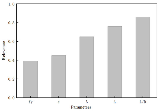
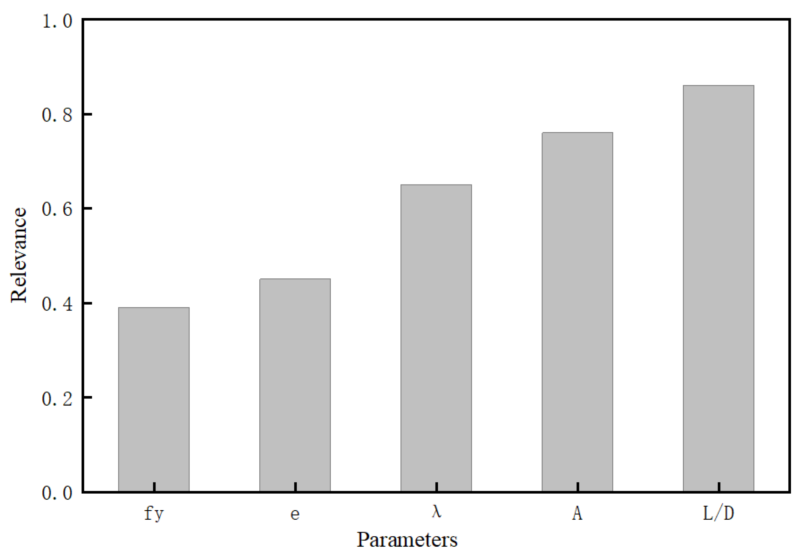
The experimental data above summarise eight factors influencing the bearing capacity. To simplify the model, the ratio method is employed to reduce the number of influencing factors to five, as follows: 1. Slenderness ratio $\mathsf{\lambda }$; 2. Yield strength fy (MPa); 3. Cross-sectional area A (mm²); 4. Diameter-to-thickness ratio L/D; 5. Eccentricity e (mm).

The correlation coefficients (r) between each influencing factor and the load-bearing capacity are shown in Figure 9. The figure indicates that L/D has the greatest influence on the output parameter, followed by A. $\mathsf{\lambda }$ ranks third, followed by e and fy.

Figure 9. Sensitivity analysis of influencing factors.

The cosine amplitude method essentially quantifies the normalised linear correlation between input features and the target variable.

3.4. Database Partitioning Strategy

To ensure consistency in the distribution of target values (load-bearing capacity) across subsets, an optimised data-partitioning strategy was adopted. First, all 236 samples from the literature database were sorted in ascending order of their target values. Subsequently, systematic sampling was performed in increments of four, where one sample from every four was assigned to the test set (25%), and the remaining 75% constituted the training set. To enhance model robustness and optimise hyperparameters, a 5-fold cross-validation (5-fold CV) was implemented within the training set. Finally, both subsets were randomly shuffled to eliminate sequence correlation. Notably, the experimental results of the axial and eccentric compression tests conducted in this study were strictly reserved as a completely independent validation set to verify the model’s final accuracy and generalisation performance.

4. Model Comparison

To verify the superior performance of the proposed model, this paper conducts a systematic comparison with prediction models based on current mainstream algorithms. This section first introduces traditional machine learning algorithms, then outlines the evaluation methods, and finally demonstrates the superiority of the proposed method in terms of prediction accuracy through the model’s prediction results.

To ensure a fair and reproducible comparison, all benchmark models (BP, KNN, RF and conventional GPR) were trained and evaluated under identical experimental settings: the same training/test split (177/59), the same preprocessing pipeline, and the same external validation set (10 specimens). Their hyperparameters were systematically determined as follows: the BP architecture and training parameters (hidden-layer size, learning rate and regularisation coefficient) were optimised via grid search with 5-fold cross-validation; the KNN neighbour number was determined by cross-validation (Section 4.2); the RF tree number and maximum depth were optimised via grid search with 5-fold cross-validation; and the conventional GPR kernel hyperparameters were optimised by maximising the log-marginal likelihood (LML) using the L-BFGS-B algorithm.

4.1. BP

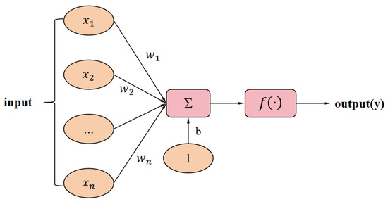
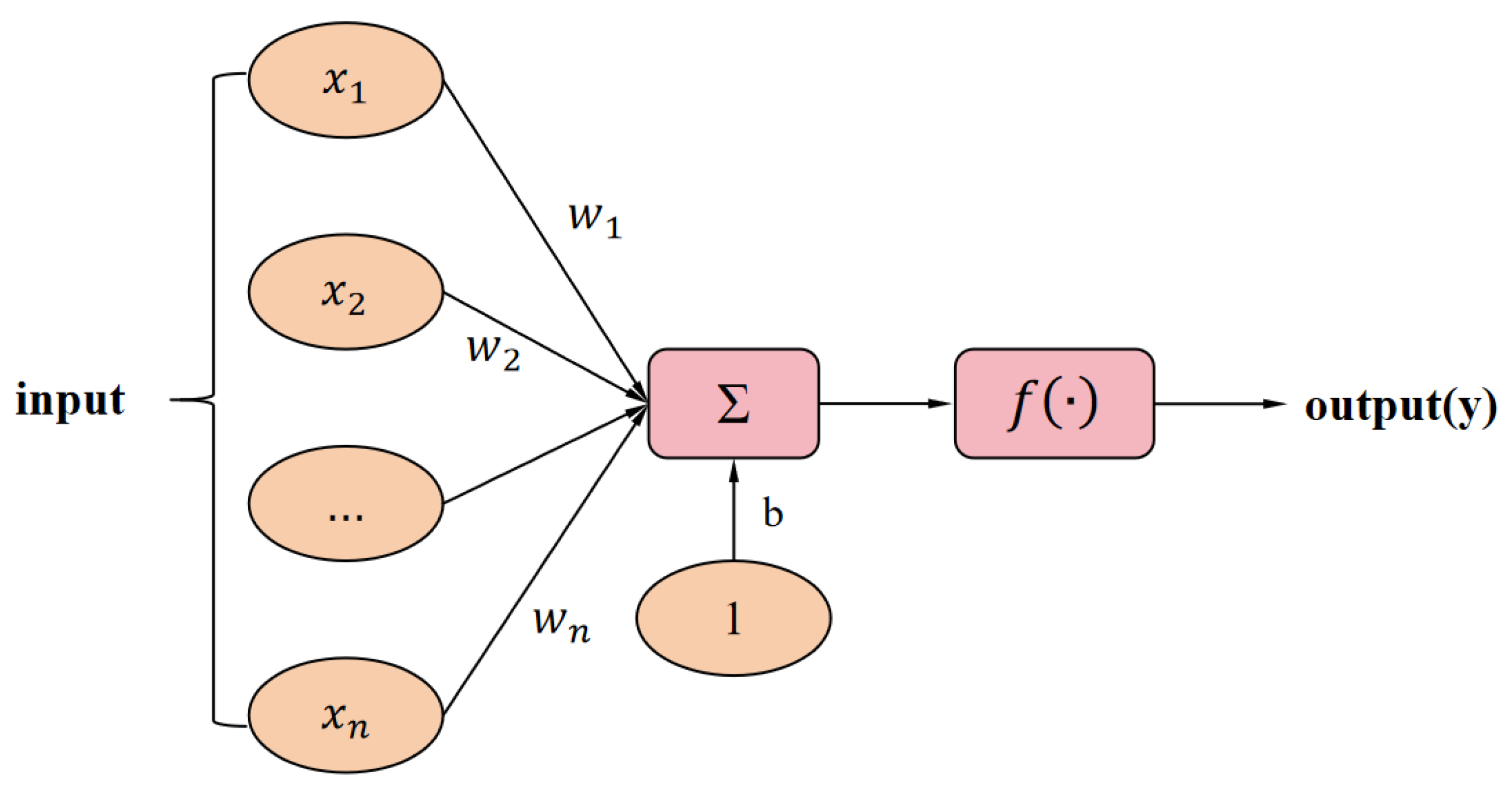
A neural network is an information-processing network system. Within this system, neurones are interconnected to facilitate complex information transmission, enabling the resolution of complex problems that traditional algorithms cannot solve [51]. The mechanism by which each neurone functions is shown in Figure 10.

Figure 10. Mathematical model of neurones.

A neural network comprises three layers: the input layer, the hidden layers and the output layer. Information processed by one neurone is fed as input to the next neurone, and this process continues until the information passes through the final neurone. Activation functions introduce nonlinear elements into the neural network, enabling it to solve complex problems that linear models cannot address and significantly enhancing the model’s learning capabilities.

4.2. KNN

KNN [48] is a supervised machine learning algorithm used for classification and regression tasks. In this method, the predicted value for a sample is calculated as the average of the output values from the k nearest neighbours in the training set. When using KNN for prediction, all training data points must be taken into account. The expression for KNN regression is defined by Equation (16), where ${\mathrm{y}}_{\mathrm{i}}$ denotes the output value of the i-th neighbour.

$$\mathrm{f}(\mathrm{x})={\displaystyle \frac{{\displaystyle {\sum }_{\mathrm{i}=1}^{\mathrm{n}}}{\mathrm{y}}_{\mathrm{i}}}{\mathrm{n}}}$$

(16)

The value of k has a significant impact on the predictions of the KNN model. Selecting a smaller k value corresponds to a smaller neighbourhood, which may lead to a higher risk of overfitting and an increase in the overall model complexity. Conversely, selecting a larger k value results in a larger neighbourhood, thereby reducing estimation errors during model training. However, for test samples that are far from the training instances, this also introduces larger prediction errors. To strike a balance between these factors, cross-validation was used to determine that k should be set to 5.

4.3. Random Forest

Random Forest [52] is a form of bagging ensemble learning. Bagging allows for the parallel training of base learners, with the aim of improving the performance of the ensemble model by reducing the variance of the base learners. Decision trees are commonly used as base learners in Random Forests. In a Random Forest, each decision tree is trained independently and is allowed to grow to its maximum size without pruning. Each decision tree makes an individual prediction, and the final collective decision is determined by a voting process based on the predictions of each tree. When making predictions using a Random Forest, n trees are constructed. Given input features ${\mathrm{x}}_1, {\mathrm{x}}_2,{\mathrm{x}}_3, \text{…}$, the Random Forest prediction model can be expressed as:

$$\mathrm{f}={\displaystyle \frac{1}{\mathrm{n}}}{\displaystyle \sum _{\mathrm{i}=1}^{\mathrm{n}}}{\mathrm{f}}_{\mathrm{i}}({\mathrm{x}}_1,{\mathrm{x}}_2,{\mathrm{x}}_3,\dots )$$

(17)

Here, f denotes the predicted output value, and ${\mathrm{f}}_{\mathrm{i}}$ denotes the prediction function of the i-th tree. The main steps of RF are as follows [53,54]:

(1)

Using the bagging method, samples are randomly drawn from the original training set to construct $\mathrm{k}$ subsets of samples.

(2)

Using the random subspace method, $\mathrm{F}$ features are randomly selected from all $\mathrm{X}$ feature attributes for node splitting to construct a single regression decision tree.

(3)

Steps (1) and (2) are repeated to construct multiple regression decision trees, maximising the growth of each tree to form a forest.

(4)

Based on the principle of ensemble learning, the mean of each regression decision tree is taken as the predicted result, expressed by the formula:

$${\overline{\mathrm{h}}}_{\mathrm{R}\mathrm{F}}(\mathrm{x})={\displaystyle \frac{1}{\mathrm{T}}}{\displaystyle \sum _{\mathrm{t}=1}^{\mathrm{T}}}\{\mathrm{h}(\mathrm{x},{\mathsf{\theta }}_{\mathrm{t}})\}$$

(18)

4.4. Performance Evaluation

To assess the accuracy of the models, we used the following three metrics [55,56] to evaluate the performance of each model: (1) the coefficient of determination (R²), (2) the root mean square error (RMSE), and (3) the mean absolute error (MAE). The mathematical formulas are as follows:

$${\mathrm{R}}^2=1-{\displaystyle \frac{{\displaystyle {\sum }_{\mathrm{j}=1}^{\mathrm{m}}}({\check{\mathrm{y}}}_{\mathrm{j}}-{\mathrm{y}}_{\mathrm{j}}{)}^2}{{\displaystyle {\sum }_{\mathrm{j}=1}^{\mathrm{m}}}({\check{\mathrm{y}}}_{\mathrm{j}}-\overline{\mathrm{y}}{)}^2}}$$

(19)

$$\mathrm{R}\mathrm{M}\mathrm{S}\mathrm{E}=\sqrt{{\displaystyle \frac{{\displaystyle {\sum }_{\mathrm{j}=1}^{\mathrm{m}}}({\check{\mathrm{y}}}_{\mathrm{j}}-{\mathrm{y}}_{\mathrm{j}}{)}^2}{\mathrm{m}}}}$$

(20)

$$\mathrm{M}\mathrm{A}\mathrm{E}={\displaystyle \frac{{\displaystyle {\sum }_{\mathrm{j}=1}^{\mathrm{m}}}|{\check{\mathrm{y}}}_{\mathrm{j}}-{\mathrm{y}}_{\mathrm{j}}|}{\mathrm{m}}}$$

(21)

In theory, the lower the RMSE and MAE, the more accurate the evaluation. The R² value ranges from 0 to 1. When the model approaches 1, its predictive ability is good; when it approaches 0, its predictive performance is poor. These performance metrics serve as good indicators of overall predictive accuracy.

4.5. Comparison of Results

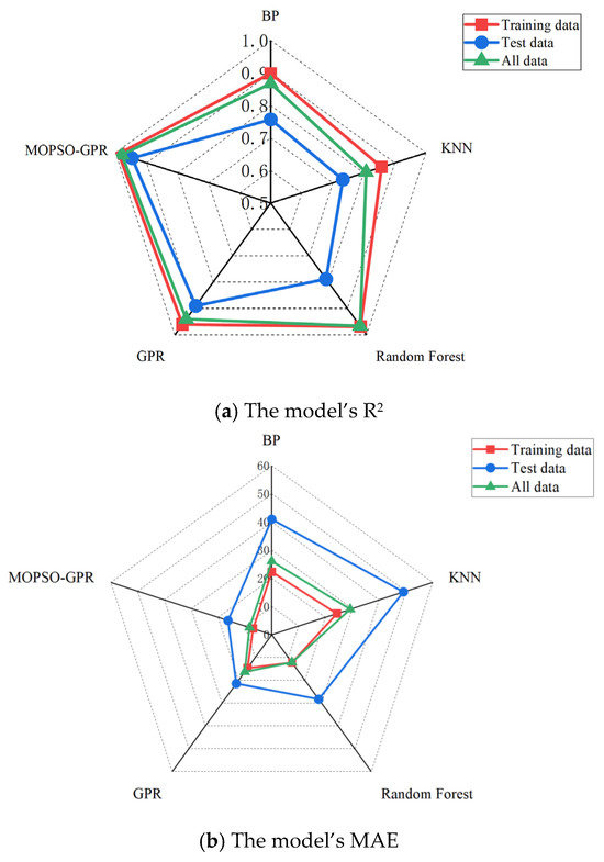
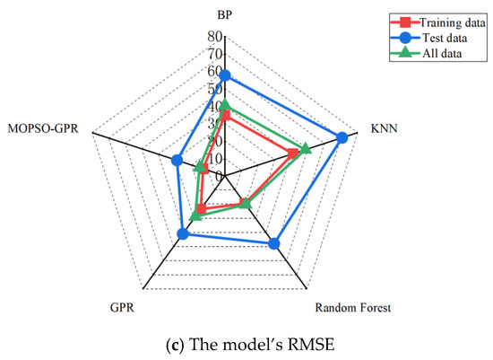
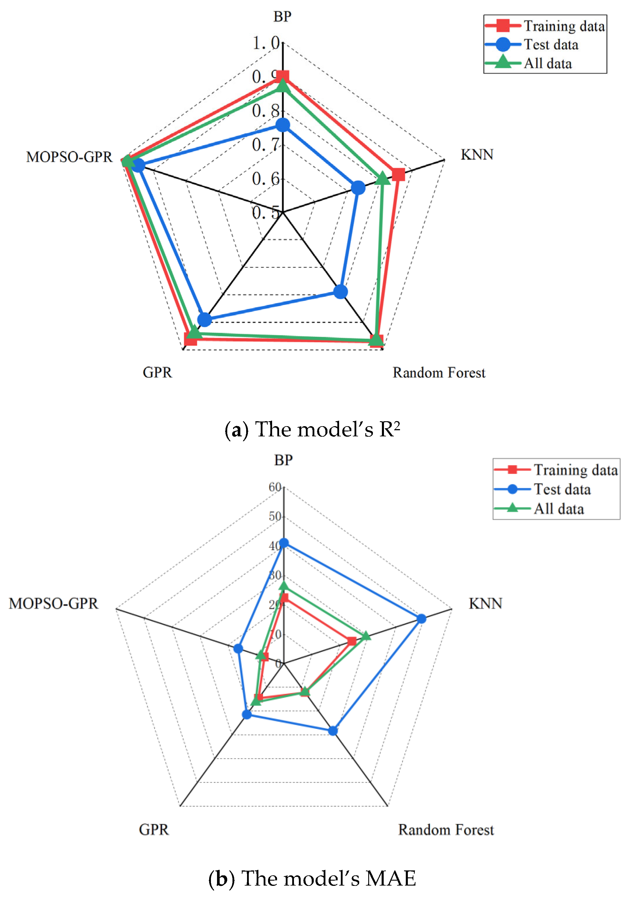
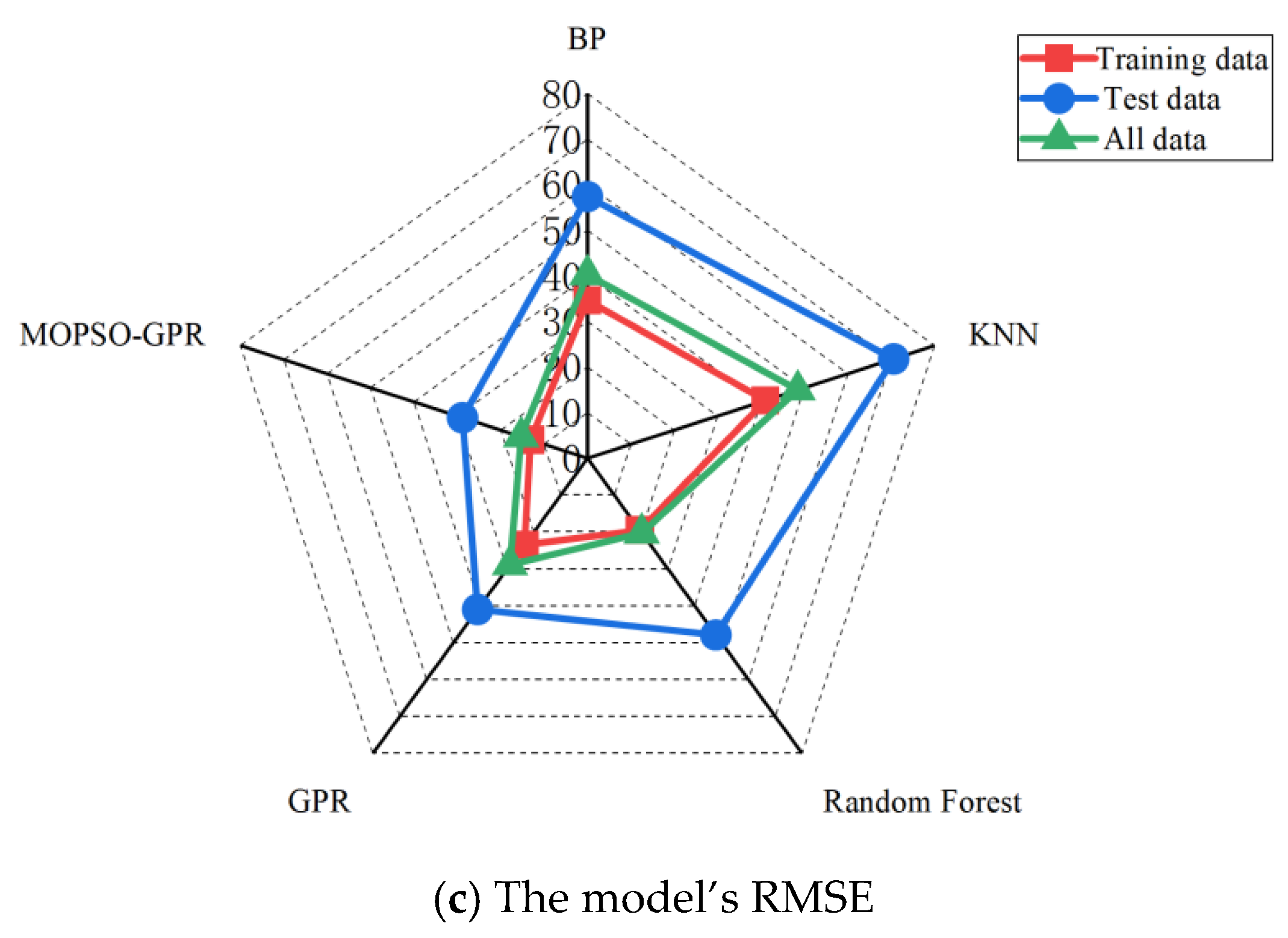
Several evaluation metrics were used to assess the performance of the above machine learning models, including MAE, RMSE and R². Compared with the KNN model, the performance of the improved GPR model increased significantly by 59.18%, as can be seen from the RMSE values in Figure 11 and Table 5. The traditional GPR model followed closely behind, demonstrating the second-best predictive performance, with an improvement of 41.91% over the KNN model. Compared to the KNN model, the Random Forest model also demonstrated a substantial performance improvement of 32.11%. Finally, the performance of the BP model improved by 18.57% compared to the KNN model. Among the five machine learning models evaluated—including the improved GPR, traditional GPR, KNN, Random Forest and BP—the improved GPR model outperformed the others in terms of predictive accuracy, as indicated by the R² values. The R² values for the improved GPR, traditional GPR, KNN, Random Forest and BP models were 0.95, 0.89, 0.73, 0.79 and 0.76, respectively. These five machine learning models exhibited different MAE values on the general-purpose database. The MAE values for the improved GPR, traditional GPR, KNN, Random Forest and BP models are 16.30, 21.42, 49.07, 28.28 and 40.97, respectively. The machine learning models were evaluated using three evaluation metrics, all of which consistently indicate that the improved GPR model outperforms the other four models under consideration.

Figure 11. Comparison of model errors.

Table 5. Different model error evaluation results.

Model	Training Data			Test Data			Validation Data			All Data
	R2	MAE	RMSE	R2	MAE	RMSE	R2	MAE	RMSE	R2	MAE	RMSE
MOPSO-GPR	0.99	6.96	13.10	0.95	16.30	28.80	0.85	12.18	27.30	0.98	8.30	15.30
GPR	0.96	14.61	23.45	0.89	21.42	40.98	0.91	77.28	77.28	0.94	16.30	28.85
KNN	0.86	24.24	41.06	0.73	49.07	70.55	0.62	47.68	58.04	0.81	29.25	48.48
Random Forest	0.97	12.20	19.52	0.79	28.28	47.90	0.53	42.74	73.78	0.97	12.13	20.26
BP	0.90	22.30	34.63	0.76	40.97	57.41	0.73	72.71	91.53	0.87	26.09	40.28

To assess the overfitting of the MOPSO-GPR model, R² was used as an evaluation metric. If the R² values on the training and test sets are similar, the model does not exhibit overfitting. In this study, the R² values on the training and test sets were 0.9898 and 0.9466, respectively, indicating that neither overfitting nor underfitting occurred.

In summary, this chapter systematically compared the proposed improved GPR model with the BP neural network, KNN, Random Forest and the traditional GPR model using three metrics: R², RMSE and MAE. The results indicate that the improved GPR model demonstrates significantly higher predictive accuracy than the comparison models (with R² reaching 0.95 and MAE reduced to 16.30), representing a 59.18% improvement in performance compared to KNN. Furthermore, with R² values of 0.9898 and 0.9466 for the training and test sets, respectively, there is no evidence of overfitting or underfitting, thereby validating the model’s superiority in terms of predictive accuracy and generalisation capability.

5. Modification of the Bearing Capacity Formula Based on MOPSO-GPR

Based on the prediction results from the MOPSO-GPR model, this chapter revises the load-bearing capacity calculation formula for aluminium alloy columns in the current code, with a particular focus on addressing prediction errors under eccentrically compressed conditions, in order to improve the formula’s predictive accuracy and engineering applicability.

5.1. Current Standard Formula

Researchers in various countries have proposed different formulas for calculating the load-bearing capacity of aluminium alloy columns. Among these, the formulas set out in the Chinese standards, the American ACI standards and the European standards are the most widely used.

5.1.1. Chinese Standards

According to the Chinese standard [5], the formula for calculating the axial compressive strength of aluminium alloy members is as follows:

$$\mathrm{N}={\mathrm{f}}_{0.2}{\mathsf{\eta }}_{\mathrm{e}}{\mathsf{\eta }}_{\mathrm{h}\mathrm{a}\mathrm{z}}\mathrm{\phi }\mathrm{A}$$

(22)

Taking into account the additional bending moments and second-order effects caused by eccentric loading, the overall stability of aluminium alloy compression–bending members is verified using the interaction equation:

$${\displaystyle \frac{\mathrm{N}}{\mathsf{\varphi }\mathrm{A}\mathrm{f}}}+{\displaystyle \frac{{\mathsf{\beta }}_{\mathrm{m}}\mathrm{M}}{\mathrm{W}\mathrm{f}(1-\mathrm{N}/{\mathrm{N}}_{\mathrm{E}})}}\le 1.0$$

(23)

5.1.2. European Standards

In accordance with the relevant provisions of EN 1999 [4], the design buckling resistance N_b,Rd for compressed members shall be taken as:

$${\mathrm{N}}_{\mathrm{b},\mathrm{R}\mathrm{d}}=\mathsf{\kappa }\mathsf{\chi }{\mathrm{A}}_{\mathrm{e}\mathrm{f}\mathrm{f}}{\mathrm{f}}_0/{\mathsf{\gamma }}_{\mathrm{M}1}$$

(24)

In this equation, $\mathsf{\chi }$ is the reduction factor corresponding to the buckling mode, which can be calculated using Equation (25); $\mathsf{\kappa }$ is the factor accounting for the effects of weld weakening; and ${\mathrm{A}}_{\mathrm{eff}}$ is the effective area for Class 4 sections after taking local buckling into account; for Class 1, 2 and 3 sections, ${\mathrm{A}}_{\mathrm{eff}} = \mathrm{A}$. For axial compression of a member, the value of $\mathsf{\chi }$ corresponding to an appropriate value of $\overline{\mathsf{\lambda }}$ shall be determined from the relevant buckling curves using the following formula:

$$\mathsf{\chi }={\displaystyle \frac{1}{\mathsf{\varphi }+\sqrt{{\mathsf{\varphi }}^2-{\overline{\mathsf{\lambda }}}^2}}},\mathsf{\chi }\le 1.0$$

(25)

where $\mathsf{\varphi } = 0.5\left(1 + \mathsf{\alpha }(\overline{\mathsf{\lambda }}-{\overline{\mathsf{\lambda }}}_0) + {\overline{\mathsf{\lambda }}}^2\right),\overline{\mathsf{\lambda }} =\sqrt{{\displaystyle \frac{{\mathrm{A}}_{\mathrm{eff}}{\mathrm{f}}_{0.2}}{{\mathrm{N}}_{\mathrm{cr}}}}}$; $\mathsf{\alpha }$ is the defect factor, ${\overline{\mathsf{\lambda }}}_0$ is the limit value for the horizontal flange, and ${\mathrm{N}}_{\mathrm{cr}}$ is the elastic critical force for the corresponding buckling mode based on the gross cross-section characteristics.

5.1.3. US Standards

In American standards, the design formula for compression–bending members is as follows:

$$\left|{\displaystyle \frac{{\mathrm{P}}_{\mathrm{r}}}{{\mathrm{P}}_{\mathrm{c}}}}+{\displaystyle \frac{{\mathrm{M}}_{\mathrm{r}\mathrm{x}}}{{\mathrm{M}}_{\mathrm{c}\mathrm{x}}}}+{\displaystyle \frac{{\mathrm{M}}_{\mathrm{r}\mathrm{y}}}{{\mathrm{M}}_{\mathrm{c}\mathrm{y}}}}\right|\le 1.0$$

(26)

In the equation, ${\mathrm{P}}_{\mathrm{r}}$ represents the design value of the stable axial compressive capacity, ${\mathrm{P}}_{\mathrm{c}}$ represents the ultimate value of the stable axial compressive capacity, ${\mathrm{M}}_{\mathrm{rx}}$ and ${\mathrm{M}}_{\mathrm{ry}}$ represent the design values of the bending capacity, and Mcx and Mcy represent the ultimate values of the bending capacity.

5.2. Validation of the GPR-Based Correction Formula

5.2.1. Parameter Determination

According to Section 5.2, the load-bearing capacity design formula in the Chinese standard is relatively more conservative when predicting the load-bearing capacity of most eccentrically loaded specimens. Relevant studies have shown that the accuracy of load-bearing capacity prediction models derived using the Gaussian process regression (GPR) algorithm is significantly improved. Therefore, in order to accurately calculate the load-bearing capacity of eccentrically loaded aluminium alloy columns, we have identified the influence parameter C_L/D as the most sensitive parameter in the sensitivity analysis. Building upon the formula in the Chinese standard, we have determined the influence coefficients using the MOPSO-GPR algorithm and propose the following modified formula:

$${\displaystyle \frac{\mathrm{N}}{\mathsf{\varphi }\mathrm{A}\mathrm{f}}}+{\displaystyle \frac{{\mathsf{\beta }}_{\mathrm{m}}\mathrm{M}}{\mathrm{W}\mathrm{f}(1-{\mathrm{C}}_{\mathrm{L}/\mathrm{D}}\times \mathrm{N}/{\mathrm{N}}_{\mathrm{E}})}}\le 1.0$$

(27)

The proposed correction factor $C_{L/D}$ is formulated in terms of $L/D$, enabling unified application to both square and circular columns with $D$ interpretation appropriate for each section type.

To determine the influence coefficient C_L/D for the correction formula, fitting was performed using the MOPSO-GPR algorithm. To ensure that the hyperparameter combinations produced a statistically significant improvement in the model’s generalisation performance, this study employed an optimisation strategy combining 5-fold cross-validation [57,58] with multi-objective optimisation, selecting the function of the influence parameter with the highest average accuracy. The results are shown below:

$${\mathrm{C}}_{\mathrm{L}/\mathrm{D}}=0.1158\times (\mathrm{L}/\mathrm{D})-2.50006$$

(28)

Because the coefficient was derived from a mixed-section database, it inherently averages the interactive buckling effects of both plate-type (SHS) and shell-type (CHS) local buckling, rendering the modified formula applicable to both circular and square aluminium alloy columns. The proposed correction factor C_L/D is not merely an empirical fitting coefficient; it is physically anchored in the second-order stability theory of beam-columns.

The factor C_L/D quantifies the deviation of the actual second-order amplification from the idealised elastic value. When C_L/D < 1.0, it indicates that the true second-order effect is less severe than the code prediction for certain slenderness ranges, implying that the original interaction equation is overly conservative; conversely, when C_L/D > 1.0, it captures enhanced second-order sensitivity due to local buckling-induced stiffness degradation. The linear form C_L/D = 0.1158(L/D) − 2.50006 emerges from the MOPSO-GPR optimisation over the mixed-section database; its linearity is theoretically justified within the investigated parametric window. In this regime, the interaction between local plate buckling (for SHSs) or shell-type ovalisation (for CHSs) and global flexural buckling produces a nearly linear variation in the effective stiffness reduction, which is reflected in the linear trend of C_L/D.

5.2.2. Analysis of Prediction Results

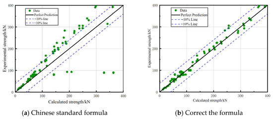
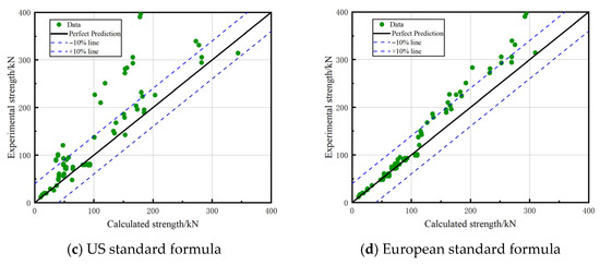
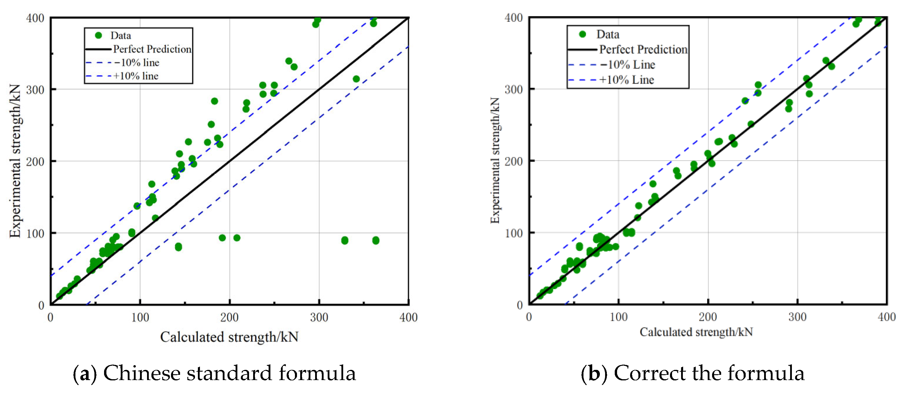
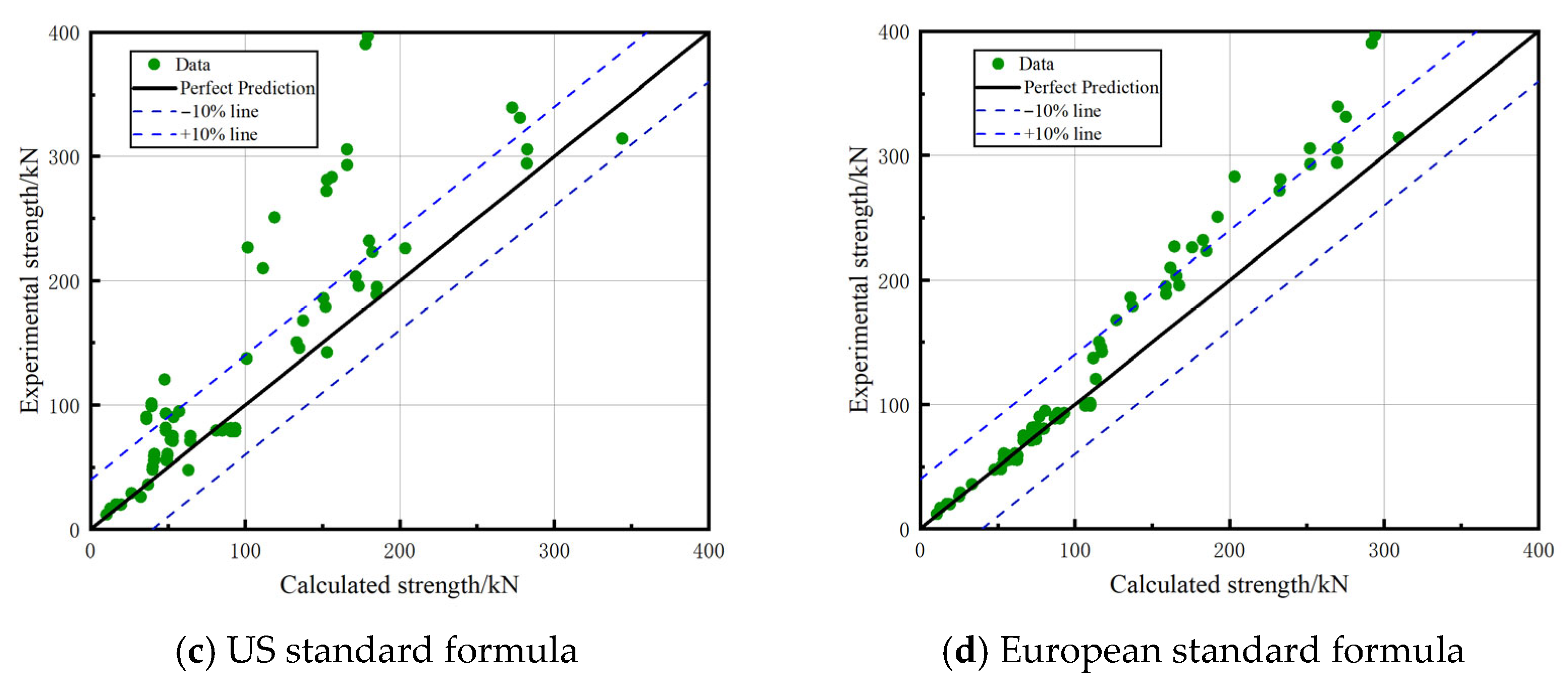
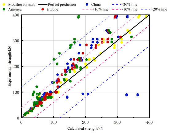
To provide a visual comparison of the accuracy of the bearing capacity prediction model proposed in this paper and that of traditional empirical models, Figure 12 presents regression plots of the calculated and experimental values for various countries. Figure 13 shows that the data values calculated using the bearing capacity prediction model proposed in this paper correspond most closely to the experimental values. In other words, all data points representing the ratio of calculated values to actual values are located around the line y = x, with the error kept within ±10%.

Figure 12. The calculated and experimental values for various countries.

Figure 13. Regression plot between calculated values and actual values of formulas and modified formulas in various countries.

The model evaluation coefficients are shown in Table 4. The statistical results in Table 6 indicate that, compared with the traditional standard, the modified formula reduces the root mean square error (RMSE) by 70.91% (from 48.30 kN to 14.05 kN) and the mean absolute error (MAE) by 70.85% (from 35.44 kN to 10.33 kN), whilst the coefficient of determination (R²) increased by 21.25%. This improvement in accuracy is not only reflected in the mean values; more importantly, the reduction in the standard deviation of the error indicates that the model possesses a stable predictive capability for aluminium alloy column specimens. It also significantly outperforms the prediction results of codes from various countries. Therefore, compared with traditional empirical models, the load-bearing capacity prediction model is more suitable for calculating the load-bearing capacity of aluminium alloy columns.

Table 6. Model error evaluation results.

Model	Dataset
	R2	RMSE (kN)	MAE (kN)
China standard formula	0.8107	48.30	35.44
Correct the formula	0.9830	14.05	10.33
European standard formula	0.9161	31.62	20.19
US standard formula	0.6986	59.95	39.92

In summary, as can be seen from the results in Figure 13, the data points calculated by the load-bearing capacity prediction model proposed in this paper are concentrated within a ±10% error margin, whereas the calculation errors of various empirical formulas from around the world are significantly larger, as evidenced by the scattered data points, which are generally distributed around a ±30% error margin. Consequently, the load-bearing capacity prediction model based on the Gaussian process regression algorithm proposed in this paper demonstrates superior accuracy to traditional empirical formulas.

6. Conclusions

In this study, a hybrid MOPSO-GPR model is proposed to predict the ultimate strength of aluminium alloy columns. This study investigates the interactive buckling failure of aluminium alloy columns under axial and eccentric compression. A predictive model was developed using a database of 236 specimens compiled from the existing literature, and its accuracy was validated against experimental results from 10 square hollow section (SHS) column specimens designed and tested in the present study. A database comprising experimental results and 236 data samples collected from the existing literature was used to construct the model, and explicit formulas for calculating the load-bearing capacity of aluminium alloy columns are presented. The load-bearing capacity prediction model proposed in this paper accounts for the influence of different stress states on load-bearing capacity and modifies the eccentric compression load-bearing capacity formulae in existing codes. For aluminium alloy columns under different loading conditions, the proposed model is compared with traditional empirical models using the coefficient of determination, mean absolute error and root mean square error as evaluation criteria.

Based on the results of the comparative analysis, the following conclusions can be drawn:

• Compared with the traditional GPR model, the MOPSO-GPR model exhibits superior predictive performance. The R², MAE and RMSE indices of the proposed MOPSO-GPR model are 0.95, 16.30, and 28.80, respectively, indicating that replacing marginal likelihood maximisation with the MOPSO algorithm can effectively enhance the performance of the GPR model.
• Compared with traditional empirical models, the proposed bearing capacity prediction model fully accounts for the influence of different loading conditions on the bearing capacity of aluminium alloy columns and provides explicit formulae.
• The error between the data generated by the proposed bearing capacity prediction model and the experimental values is within 10%, which is smaller than the error between traditional empirical models and experimental data. Therefore, the proposed bearing capacity prediction model is more suitable for calculating the bearing capacity of aluminium alloy columns under eccentric loading conditions.

References

- Georgantzia, E.; Gkantou, M.; Kamaris, G.S. Aluminium alloys as structural material: A review of research. Eng. Struct. 2021, 227, 111372. [Google Scholar] [CrossRef] [Scilit]
- Mavhungu, S.T.; Akinlabi, E.T.; Onitiri, M.A.; Varachia, F.M. Aluminum Matrix Composites for Industrial Use: Advances and Trends. Procedia Manuf. 2017, 7, 178–182. [Google Scholar] [CrossRef] [Scilit]
- You, X.; Xing, Z.; Jiang, S.; Zhu, Y.; Lin, Y.; Qiu, H.; Nie, R.; Yang, J.; Hui, D.; Chen, W.; et al. A review of research on aluminum alloy materials in structural engineering. Dev. Built Environ. 2024, 17, 100319. [Google Scholar] [CrossRef] [Scilit]
- EN 1999-1-1; Eurocode 9—Design of Aluminium Structures—Part 1-1: General Rules. European Committee for Standardization: Brussels, Belgium, 2023; p. 373.
- GB 50429-2007; Ministry of Housing and Urban-Rural Development of China (MOHURD). Code for Design of Aluminium Structures; China Architecture & Building Press: Beijing, China, 2007; p. 72.
- Mazzolani, F. Structural Applications of Aluminium in Civil Engineering. Struct. Eng. Int. 2006, 16, 280–285. [Google Scholar] [CrossRef] [Scilit]
- Su, M.-N.; Young, B.; Gardner, L. Testing and Design of Aluminum Alloy Cross Sections in Compression. J. Struct. Eng. 2014, 140, 04014047. [Google Scholar] [CrossRef] [Scilit]
- Wang, Y.; Chen, B.; Dai, P.; Wang, Y.; Song, Y.; Jiang, K.; Hai, L. Experimental and numerical study on lateral-torsional buckling of welded QN1803 high-strength stainless steel I-girders. Thin-Walled Struct. 2025, 212, 113190. [Google Scholar] [CrossRef] [Scilit]
- Wang, Y.; Chen, B.; Dai, P.; Chen, Y.; Zhang, Z.; Lu, P.; Huang, C. Design recommendations for perforated S32001 high-strength stainless steel girders under concentrated loading. Structures 2025, 78, 109295. [Google Scholar] [CrossRef] [Scilit]
- Li, L.; Dahboul, S.; Verma, P.; Dey, P.; Fafard, M.; Boissonnade, N. An Experimental Study on the Local Instability of Aluminum Circular Hollow Sections. In Proceedings of the Canadian Society for Civil Engineering Annual Conference; Springer Nature: Cham, Switzerland, 2023; pp. 295–305. [Google Scholar]
- Rong, B.; Zhang, Y.; Zhang, S.; Li, Z. Experiment and numerical investigation on the buckling behavior of 7A04-T6 aluminum alloy columns under eccentric load. J. Build. Eng. 2022, 45, 103625. [Google Scholar] [CrossRef] [Scilit]
- Zhao, Y.; Zhai, X.; Wang, J. Buckling behaviors and ultimate strengths of 6082-T6 aluminum alloy columns under eccentric compression—Part I: Experiments and finite element modeling. Thin-Walled Struct. 2019, 143, 106207. [Google Scholar] [CrossRef] [Scilit]
- He, J.; Liu, Y.; Hong, Q.; Li, R.; Gao, R.; Fu, B.; Ding, L.; Dai, X. Axial Compressive Behavior of Square Double-Skin Hybrid Concrete Bar Columns with Small-Diameter Concrete-Infilled GFRP Tubes. Buildings 2025, 15, 3888. [Google Scholar] [CrossRef] [Scilit]
- Zhang, Z.; Yuan, P.; Chen, L. Experimental and Numerical Study of the Seismic Behavior of Single-Plane Trussed CFSST Composite Column Frames. Buildings 2026, 16, 114. [Google Scholar] [CrossRef] [Scilit]
- Chou, J.-S.; Tsai, C.-F. Concrete compressive strength analysis using a combined classification and regression technique. Autom. Constr. 2012, 24, 52–60. [Google Scholar] [CrossRef] [Scilit]
- Devaney, R.; Padraic, O.D.; Leen, S. Global and local fatigue analysis of X100 and X60 steel catenary riser girth welds. J. Struct. Integr. Maint. 2017, 2, 181–189. [Google Scholar] [CrossRef] [Scilit]
- Yaseen, Z.M.; Deo, R.C.; Hilal, A.; Abd, A.M.; Bueno, L.C.; Salcedo-Sanz, S.; Nehdi, M.L. Predicting compressive strength of lightweight foamed concrete using extreme learning machine model. Adv. Eng. Softw. 2018, 115, 112–125. [Google Scholar] [CrossRef] [Scilit]
- Zhang, B.; Phillips, D.V.; Wu, K. Effects of loading frequency and stress reversal on fatigue life of plain concrete. Mag. Concr. Res. 1996, 48, 361–375. [Google Scholar] [CrossRef] [Scilit]
- Zhong, C.-J.; Feng, R.-Q.; Zhang, Z.-J. Prediction of Ultimate Bearing Capacity and Structural Optimization of Aluminum Alloy Plate Joints Based on Artificial Neural Network. Int. J. Steel Struct. 2021, 21, 1759–1774. [Google Scholar] [CrossRef] [Scilit]
- Mo, C.; Huang, J.; Huang, J.; Li, T.; Yang, Y. Prediction of Flexural Bearing Capacity of Aluminum-Alloy-Reinforced RC Beams Based on Machine Learning. Symmetry 2025, 17, 944. [Google Scholar] [CrossRef] [Scilit]
- Dalmasso, M.; Civera, M.; De Biagi, V.; Chiaia, B. Gaussian Process Regression (GPR)-based missing data imputation and its uses for bridge structural health monitoring. Adv. Bridge Eng. 2025, 6, 23. [Google Scholar] [CrossRef] [Scilit]
- Asteris, P.G.; Kolovos, K.G. Self-compacting concrete strength prediction using surrogate models. Neural Comput. Appl. 2019, 31, 409–424. [Google Scholar] [CrossRef] [Scilit]
- Emad, W.; Mohammed, A.S.; Bras, A.; Asteris, P.G.; Kurda, R.; Muhammed, Z.; Hassan, A.M.T.; Qaidi, S.M.A.; Sihag, P. Metamodel techniques to estimate the compressive strength of UHPFRC using various mix proportions and a high range of curing temperatures. Constr. Build. Mater. 2022, 349, 128737. [Google Scholar] [CrossRef] [Scilit]
- Emad, W.; Salih Mohammed, A.; Kurda, R.; Ghafor, K.; Cavaleri, L.; Qaidi, S.M.A.; Hassan, A.M.T.; Asteris, P.G. Prediction of concrete materials compressive strength using surrogate models. Structures 2022, 46, 1243–1267. [Google Scholar] [CrossRef] [Scilit]
- Nguyen, N.-H.; Vo, T.P.; Lee, S.; Asteris, P.G. Heuristic algorithm-based semi-empirical formulas for estimating the compressive strength of the normal and high performance concrete. Constr. Build. Mater. 2021, 304, 124467. [Google Scholar] [CrossRef] [Scilit]
- Sun, B.; Yao, H.-T. The short-term wind speed forecast analysis based on the PSO-LSSVM predict model. Power Syst. Prot. Control 2012, 40, 85–89. [Google Scholar]
- Moayedi, H.; Mehrabi, M.; Mosallanezhad, M.; Rashid, A.S.A.; Pradhan, B. Modification of landslide susceptibility mapping using optimized PSO-ANN technique. Eng. Comput. 2019, 35, 967–984. [Google Scholar] [CrossRef] [Scilit]
- Alimoradi, A.; Beck James, L. Machine-Learning Methods for Earthquake Ground Motion Analysis and Simulation. J. Eng. Mech. 2015, 141, 04014147. [Google Scholar] [CrossRef] [Scilit]
- Hamrouche, R.; Klysz, G.; Balayssac, J.-P.; Rhazi, J.; Ballivy, G. Numerical Simulations and Laboratory Tests to Explore the Potential of Ground-Penetrating Radar (GPR) in Detecting Unfilled Joints in Brick Masonry Structures. Int. J. Archit. Herit. 2012, 6, 648–664. [Google Scholar] [CrossRef] [Scilit]
- Pereira Dias, P.; Bhagya Jayasinghe, L.; Waldmann, D. Machine learning in mix design of Miscanthus lightweight concrete. Constr. Build. Mater. 2021, 302, 124191. [Google Scholar] [CrossRef] [Scilit]
- Seeger, M. Gaussian Processes for Machine Learning. Int. J. Neural Syst. 2008, 14, 69–106. [Google Scholar] [CrossRef] [Scilit] [PubMed]
- Zhang, H.; Wu, Y.; Yang, S. Probabilistic analysis of tunnel convergence in spatially variable soil based on Gaussian process regression. Eng. Appl. Artif. Intell. 2024, 131, 107840. [Google Scholar] [CrossRef] [Scilit]
- GB/T 228.1-2021; State Administration for Market Regulation (SAMR); Standardization Administration of China (SAC). Metallic Materials—Tensile Testing—Part 1: Method of Test at Room Temperature. China Standards Press: Beijing, China, 2021.
- JGJ/T 101-2015; Ministry of Housing and Urban-Rural Development of the People’s Republic of China. Specification for Seismic Test of Buildings. China Architecture & Building Press: Beijing, China, 2015.
- Guo, X. Theoretical and Experimental Study on Aluminum Alloy Structural Components. Ph.D. Thesis, Tongji University, Shanghai, China, 2006. [Google Scholar]
- Guo, X.; Shen, Z.; Li, Y.; Qiu, Z.; Yao, N. Theoretical and Experimental Study on Aluminum Alloy Eccentric Compression Members. J. Struct. Eng. 2007, 6, 136–146. [Google Scholar] [CrossRef]
- Li, M.; Chen, Y.J.; Qian, R.J.; Yao, N.L. Experimental Study on the Stability Coefficient of Circular Tubular Aluminium Alloy Axial Compression Members. Spat. Struct. 2000, 1, 59–64+53. [Google Scholar] [CrossRef]
- Li, X. A Study on the Static Load-Bearing Capacity of Axially Compressed Aluminum Alloy Round Tubular Members. Master’s Thesis, Xi’an University of Architecture and Technology, Xi’an, China, 2004. [Google Scholar]
- Zhang, D. Study on the Local Stability of Hollow Aluminum Alloy Short Columns Under Axial Compression. Master’s Thesis, Shenyang Jianzhu University, Shenyang, China, 2023. [Google Scholar]
- Zheng, Z.Y. Study on the Mechanical Properties and Reliability Analysis of 6082-T6 Aluminum Alloy Members Subjected to Bending and Shear; Harbin Institute of Technology: Harbin, China, 2020. [Google Scholar]
- Zhou, F.; Young, B. Aluminum tubular sections subjected to web crippling—Part I: Tests and finite element analysis. Thin-Walled Struct. 2008, 46, 339–351. [Google Scholar] [CrossRef] [Scilit]
- Zhu, J.-H.; Young, B. Experimental investigation of aluminum alloy circular hollow section columns. Eng. Struct. 2006, 28, 207–215. [Google Scholar] [CrossRef] [Scilit]
- Zhu, J.-H.; Young, B. Tests and Design of Aluminum Alloy Compression Members. J. Struct. Eng. 2006, 132, 1096–1107. [Google Scholar] [CrossRef] [Scilit]
- Zhu, J.-H.; Young, B. Aluminum alloy circular hollow section beam-columns. Thin-Walled Struct. 2006, 44, 131–140. [Google Scholar] [CrossRef] [Scilit]
- Zhang, M.; Wu, D.; Xiang, H.; Li, X. Experiment research on stability factor for circular section aluminum alloy members under axially compressive load. J. Chang. Univ. (Archit. Environ. Sci. Ed.) 2004, 21, 34–38. [Google Scholar]
- Guillow, S.R.; Lu, G.; Grzebieta, R.H. Quasi-static axial compression of thin-walled circular aluminium tubes. Int. J. Mech. Sci. 2001, 43, 2103–2123. [Google Scholar] [CrossRef] [Scilit]
- Jayalakshmi, T.; Santhakumaran, A. Statistical normalization and back propagation for classification. Int. J. Comput. Theory Eng. 2011, 3, 1793–8201. [Google Scholar]
- Pedregosa, F.; Varoquaux, G.; Gramfort, A.; Michel, V.; Thirion, B.; Grisel, O.; Blondel, M.; Müller, A.; Nothman, J.; Louppe, G.; et al. Scikit-learn: Machine Learning in Python. J. Mach. Learn. Res. 2018, 12, 2825–2830. [Google Scholar]
- Bradecki, T.; Swoboda, J.; Nowak, K.; Dziechciarz, K. Models for Experimental High Density Housing. IOP Conf. Ser. Mater. Sci. Eng. 2017, 245, 052025. [Google Scholar] [CrossRef] [Scilit]
- Peng, Z.Z.; Feng, K.; Xiao, M.Q.; He, C.; Jiang, C.; Chen, H.W. Reasonable overlying thickness of subaqueous tunnels based on pressure arch theory. Rock Soil Mech. 2018, 39, 2609–2616. [Google Scholar] [CrossRef]
- Liu, G.; Jiang, K.; Cheng, X. Recent Advances in Evolutionary Neural Networks. Control Decis. 1998, 13, 617–624. [Google Scholar]
- Breiman, L. Random Forests. Mach. Learn. 2001, 45, 5–32. [Google Scholar] [CrossRef] [Scilit]
- Daneshvar, D.; Behnood, A. Estimation of the dynamic modulus of asphalt concretes using random forests algorithm. Int. J. Pavement Eng. 2022, 23, 250–260. [Google Scholar] [CrossRef] [Scilit]
- Probst, P.; Wright, M.N.; Boulesteix, A.L. Hyperparameters and tuning strategies for random forest. Data Min. Knowl. Discov. 2018, 9, e1301. [Google Scholar] [CrossRef] [Scilit]
- Gao, H.; Cheng, H.; Cui, X. Calculation of Load-Carrying Capacity of Square Concrete Filled Tube Columns Based on Neural Network. Appl. Mech. Mater. 2013, 351–352, 713–716. [Google Scholar] [CrossRef] [Scilit]
- Nikbin, M.; Rahimi, S.; Allahyari, H. A new empirical formula for prediction of fracture energy of concrete based on the artificial neural network. Eng. Fract. Mech. 2017, 186, 466–482. [Google Scholar] [CrossRef] [Scilit]
- Ahmadi, M.; Naderpour, H.; Kheyroddin, A. Utilization of artificial neural networks to prediction of the capacity of CCFT short columns subject to short term axial load. Arch. Civ. Mech. Eng. 2014, 14, 510–517. [Google Scholar] [CrossRef] [Scilit]
- Zhao, P.; Liu, X. Risk warning model based on radial basis function neural network. In Proceedings of the 2008 7th World Congress on Intelligent Control and Automation, Chongqing, China, 25–27 June 2008; pp. 5817–5820. [Google Scholar]
Disclaimer/Publisher’s Note: The statements, opinions and data contained in all publications are solely those of the individual author(s) and contributor(s) and not of MDPI and/or the editor(s). MDPI and/or the editor(s) disclaim responsibility for any injury to people or property resulting from any ideas, methods, instructions or products referred to in the content. |
© 2026 by the authors. Licensee MDPI, Basel, Switzerland. This article is an open access article distributed under the terms and conditions of the Creative Commons Attribution (CC BY) license.