Built Environment Factors and Interventions Supporting Children’s Active School Travel: Insights from Machine Learning

Abstract

Active school travel (AST) is an important source of daily physical activity for children, yet its environmental correlates remain mixed and may be more complex than conventional linear models suggest. This study examines the associations of school-travel distance, built environment, socio-demographic attributes, and natural environment with children’s AST in Wuhan, China. Using 2020 travel survey data for children aged 6–15 and an XGBoost–SHAP framework, the study evaluates relative importance, nonlinear association patterns, and pairwise interactions among key variables. The results show that school-travel distance is the dominant correlate of AST, accounting for 44.07% of total model importance. Built-environment variables collectively contribute 36.24%, substantially exceeding socio-demographic attributes, while terrain also shows a non-negligible role. Several built-environment variables, including transit station density, road density, intersection density, land-use entropy, and POI density, display clear nonlinear patterns and directional shifts. Distance and age further condition the associations of other variables with AST, indicating substantial heterogeneity across distance bands and developmental stages. Overall, the findings suggest that AST should not be understood through average main effects alone, and that more age-sensitive, distance-sensitive, and context-specific planning strategies are needed to support child-friendly school travel.

1. Introduction

Children’s health has become a growing global concern. Regular physical activity is essential for healthy growth, musculoskeletal development, and cognitive and psychosocial well-being, yet many young people still do not meet recommended activity levels [1]. In this context, children’s school travel has attracted increasing attention because it is one of the few routine activities that can embed physical activity into daily life. Active school travel (AST), usually defined as walking or cycling to and from school, is therefore widely recognized as an important component of children’s daily physical activity and healthy urban mobility [2]. Compared with motorized school travel, AST is associated with higher overall physical activity, better fitness-related outcomes, and greater opportunities for independent mobility and social interaction in everyday life [3,4,5]. More broadly, children’s access to daily destinations through active or independent travel is also relevant to their well-being and everyday development [6].

Despite these benefits, AST has declined in many countries over recent decades, while parental chauffeuring and other motorized school trips have become increasingly common [7]. Existing studies suggest that this shift is not only related to changing family preferences, but also to wider structural processes such as rapid urban expansion, increasing home–school separation, rising private vehicle ownership, and growing traffic and safety concerns [8]. In China, for example, the prevalence of active travel to and from school dropped markedly between 1997 and 2011, and this decline was associated with both longer school distance and greater private vehicle ownership [9]. More broadly, previous work has argued that economic growth and urbanization may contribute to the decline of AST in developing countries by expanding motorized mobility and increasing spatial separation between home and school [8]. These trends suggest that, under rapid urban transformation and motorization, AST is increasingly compressed by the expansion of motorized travel.

Against this background, researchers have devoted increasing attention to the logic underlying AST. Among the many correlates identified in the literature, distance is the factor on which the strongest consensus has been reached. Across both reviews and empirical studies, home–school distance has repeatedly been identified as the strongest and most stable correlate of AST, with the likelihood of walking or cycling declining as distance increases [10,11]. This pattern has been reported in cross-sectional studies, longitudinal studies, and review articles alike [12,13].

Beyond distance, a large body of research has focused on macro-scale built-environment variables such as density, street connectivity, land-use mix, walkability, and traffic exposure [14]. However, existing findings vary across study contexts, measurement approaches, and urban environments. Some studies report that higher walkability, better connectivity, and greater land-use mix are associated with higher levels of AST [15,16,17]. For example, regularly walking to school was more common in school neighborhoods with high street connectivity and low traffic volume, and active commuting has also been linked to higher land-use mix and the presence of street trees [18]. At the same time, these relationships are not uniformly positive. The same Australian study showed that high connectivity combined with heavy traffic reduced the likelihood of walking to school [17]. Other studies found that some neighborhood or route variables were weak, unstable, or differed between the trip to school and the trip home [16,19]. A Dutch study further suggested that social neighborhood characteristics may matter as much as, or even more than, physical infrastructure alone [19]. Taken together, these findings indicate that macro-scale built-environment variables do not exert fixed positive or negative effects on AST. Their associations vary with traffic conditions, trip direction, and local context.

More recent studies have extended this literature from conventional neighborhood indicators to finer-grained route and street-level features [20,21]. Early route-based research already argued that children’s school travel should be understood through neighborhood, route, and school environments together, rather than through residential context alone. More recently, the development of street-view imagery and computer vision has provided new ways to quantify pedestrian-level environmental exposure [22]. This line of work shows that micro-scale streetscape characteristics also matter. For example, greener school surroundings have been associated with a higher likelihood of AST in Hong Kong [23], while street-view-based studies have identified salient roles for greenery, traffic lights, and other visual street attributes in predicting the propensity to walk to school [24]. These studies broaden the environmental dimension of AST research. They also suggest that what children actually perceive during walking cannot be fully represented by conventional density- or land-use-based indicators.

At the same time, the methodological development of the field help explain why empirical conclusions often vary across contexts and measurement approaches. Much of the earlier AST evidence was generated through logistic regression, multilevel regression, or structural equation modeling, and these approaches have been valuable for identifying whether a variable is positively or negatively associated with AST, or whether direct and indirect paths exist [11,25]. However, such models often summarize associations as average effects and are less suited to capturing threshold effects, nonlinear responses, and changing relationships across value ranges. In recent years, researchers have increasingly adopted nonlinear and machine-learning-based approaches to address this limitation. Using generalized additive mixed models, Wang et al. showed that several streetscape attributes were nonlinearly associated with children’s walks to school, and that these associations were further modified by socioeconomic characteristics [20]. Using street-view imagery and machine learning, Wu et al. (2023) found salient nonlinear and threshold effects of micro-level streetscape features on children’s propensity to walk to school, and showed that neglecting genuine nonlinearity may lead to misleading conclusions [24]. More recently, Tang et al. (2025) applied a gradient boosting regression tree model to children’s AST levels in a mountainous city and identified nonlinear relationships, threshold effects, and interactions involving built-environment and topographical variables [26]. Taken together, these studies suggest that environmental variables may not have a single stable direction of association. Therefore, knowing which variables are more important, or whether a single variable shows a nonlinear association, is still not enough to fully describe this complex association structure.

This leads to two gaps. First, studies that simultaneously integrate macro-scale built-environment indicators, micro-scale streetscape characteristics, and natural constraints, remain limited in AST research. Second, although research on nonlinear AST has advanced in recent years, existing studies have focused primarily on univariate response models, with little attention being paid to the interactions among variables. This is especially important for distance, which is almost universally identified as the most important correlate of AST but whose conditioning effect on the strength and direction of other environmental associations remains insufficiently understood. These gaps indicate the need for a more integrated framework that can explicitly identify nonlinearities and interactions and better capture the hierarchical, condition-dependent, and potentially interactive nature of children’s school-travel behavior. Accordingly, this study contributes to the existing literature in three aspects. First, it integrates macro-scale built-environment indicators, micro-scale streetscape attributes, and terrain within a unified analytical framework. Second, it uses SHAP interaction analysis to examine how school-travel distance and age condition the associations between environmental factors and AST, thereby moving beyond single-variable nonlinear interpretation. Third, it provides context-specific evidence from Wuhan, a large and multi-centered Chinese city.

In summary, this study investigates the associations of school-travel distance, built environment, socio-demographic attributes, and natural environment with children’s AST in Wuhan. Using 2020 travel survey data and an XGBoost–SHAP framework, the study addresses two questions. First, when a richer set of environmental variables is considered, what are the relative importance and nonlinear association patterns of these factors with AST? Second, how do key variables interact with one another, especially how does school-travel distance condition the associations between other environmental conditions and AST?

The remainder of this paper is organized as follows. Section 2 describes the materials and methods. Section 3 reports the results. Section 4 discusses the main findings and their implications. Section 5 concludes the paper.

2. Materials and Methods

2.1. Study Area and Sample Characteristics

The study focuses on the urban development area of Wuhan, China (Figure 1). Wuhan, the capital of Hubei Province, is one of the largest megacities in central China. It has a highly complex and representative transport system, characterized by cross-river bridges, a dense rail-transit network, and large daily travel volumes. These features make Wuhan an appropriate case for examining how urban spatial conditions are associated with children’s school-travel behavior.

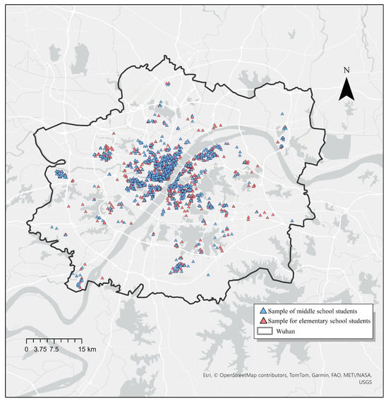
Figure 1. Study area. (Source: Created by the authors).

The individual-level sample was drawn from the 2020 Wuhan Resident Travel Survey, an official citywide survey organized by the local government and implemented by the Wuhan Institute of Transportation Development Strategy. This survey is conducted once every ten years to capture residents’ daily travel characteristics, including trip origins and destinations, trip purposes, and travel modes, together with socio-demographic information. Between October and December 2020, approximately 0.1% of the resident population was selected through random sampling, and face-to-face household interviews were conducted. The sample distribution was designed to match the actual population distribution across the city.

Based on the 2020 Wuhan Resident Travel Survey, we first selected children aged 6–15 years, corresponding to the primary- and junior-secondary-school stages of compulsory education in China. We then retained respondents whose residences were located within the Wuhan urban development area and whose reported trip purpose was school-travel. After applying these screening criteria and excluding records with missing key information, 2309 observations were retained for the final analysis (Table 1). Active school travel (AST) was coded as 1 when the reported school trip was made by walking or cycling and as 0 for all other modes. In the final sample, 1319 children (57.1%) were classified as AST and 990 (42.9%) as non-AST.

Table 1. Overall sample characteristics (N = 2309).

Variable	Description	Mean	SD	Min	Max	Variance
AST	Active school travel (1 = walking/cycling, 0 = otherwise)	0.57	0.50	0.00	1.00	0.25
School-travel distance	Euclidean distance from home to school (km)	2.40	3.81	0.10	37.10	14.52
Age	Child age (years)	10.68	2.63	6.00	15.00	6.93
Male	Gender (1 = male)	0.58	0.49	0.00	1.00	0.24
Hukou	Household registration (1 = local Hukou)	0.94	0.23	0.00	1.00	0.05
Family size	Household size (persons)	3.28	0.68	1.00	6.00	0.47
Household income	Household annual income ranges (in CNY) (1 = below 50,000; 2 = 50,000–100,000; 3 = 100,000–250,000; 4 = 250,000–400,000; 5 = 400,000–550,000; 6 = 550,000–700,000; 7 = above 700,000	2.96	0.87	1.00	7.00	0.76
House size	Housing area (m2) (1 = below 40; 2 = 40–70; 3 = 70–90; 4 = 90–110; 5 = 110–120; 6 = 120–150; 7 = above 150)	3.70	1.01	1.00	7.00	1.03

Source: Created by the authors.

2.2. Environmental Variables

All built-environment variables were measured within a 15 min, walking-scale community. Using the batch route-planning function of the Baidu Maps API, we delineated an irregular 15 min walking isochrone for each respondent on the basis of actual pedestrian routes rather than simple circular buffers. This approach follows recent work on activity-space-sensitive exposure measurement and better captures the daily built environment surrounding residents [27]. School-travel distance and built-environment exposure were used to represent different spatial constructs [28]. The former was measured as Euclidean home–school distance to capture basic spatial separation, whereas the latter was derived from 15 min network-based walking isochrones to represent accessible residential built-environment exposure.

The Wuhan GIS Open Database served as the main source for land-use information, and 2020 land-use data were used to derive the relevant land-use indicators. Population and employment data were obtained from the 2020 Population and Economic Census. Land-use entropy was calculated using an entropy index based on nine land-use categories: residential, commercial service, public administration and public service, green space and plaza, industrial, transportation, construction, warehousing, and public facilities. POI density was used as a proxy for local amenity accessibility. Following Liu et al. (2020), fine-grained POI data can capture residents’ exposure to nearby daily services more directly [29]. To reduce severe multicollinearity among amenity indicators, five daily life POI categories—dining, retail, education, recreation, and medical services—were aggregated into a single 15 min POI density measure. Intersection density and transit station density were derived from OpenStreetMap and measured as the number of intersections or transit stops per square kilometer within the isochrone. Distance to the city center was measured as the Euclidean distance from each residence to Hankou CBD, while distance to the nearest cluster center was calculated as the straight-line distance to the closest of five recognized urban cluster centers identified from 2018 LBS data [30].

At the micro scale, Baidu Street View panoramas captured in 2019 were downloaded and cropped into four directional images for each sampled location (Figure 2). Semantic segmentation was then implemented using the MMSegmentation framework with an OCRNet architecture to quantify the pixel shares of visual elements related to walking comfort and traffic safety (Figure 3). The initial candidate set covered ten visual elements, including sidewalk, sky, building, roadway, fence, traffic signs, vegetation, pedestrians, motor vehicles, and non-motor vehicles, following recent streetscape studies [22,23,31]. Candidate variables were screened to reduce redundancy and multicollinearity before model fitting. Variable retention was not based solely on statistical diagnostics, but also considered theoretical relevance to children’s active school travel and data stability [32]. For streetscape indicators, particular attention was given to visual elements that are related to walking comfort, visual enclosure, traffic exposure, and pedestrian safety. After this process, seven streetscape indicators were retained in the final model: roadway, sidewalk, building, wall, fence, vegetation, and sky.

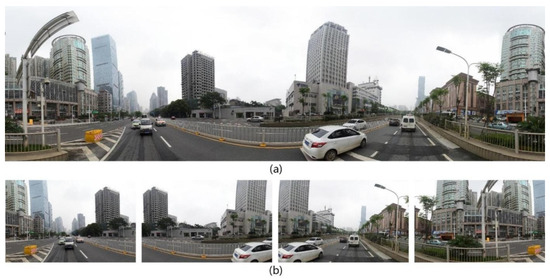
Figure 2. Street view imagery: (a) panoramic view; (b) natural view. (Source: Created by the authors).

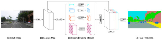
Figure 3. Illustration of the BSV-based eye-level streetscape elements estimation method. (Source: Created by the authors).

To capture topographic constraints in the school-travel environment, a terrain variable was included to describe surface relief within each respondent’s 15 min walking isochrone. This variable was derived from DEM elevation data for Wuhan and was calculated in GIS as the mean slope within the analysis unit. It reflects the potential physical burden and route resistance faced during walking or cycling. All predictors were standardized before model fitting. The final retained variables and their summary statistics are shown in Table 2.

Table 2. Definitions and summary statistics of environment variables retained in the AST model.

Variables	Description	AST Mean	AST SD	Non-AST Mean	Non-AST SD
Built environment
Distance to city center	Euclidean distance from residence to Hankou CBD (km)	5.71	3.51	7.22	3.61
Distance to cluster center	Euclidean distance from residence to the nearest identified urban cluster center (km)	3.32	1.31	3.41	1.63
Population density	Resident population density within the 15 min walking isochrone (persons/km2)	32,951.23	17,070.24	25,118.37	14,459.44
Job density	Employment density within the 15 min walking isochrone (jobs/km2)	21,899.18	9799.93	18,518.89	9160.54
Land-use entropy	Land-use mix within the 15 min walking isochrone (entropy index)	0.69	0.10	0.70	0.10
Intersection density	Street-intersection density within the 15 min walking isochrone (count/km2)	21.20	10.14	16.73	8.24
Transit station density	Transit-stop density within the 15 min walking isochrone (count/km2)	31.67	11.50	26.97	11.01
Subway station density	Metro-station density within the 15 min walking isochrone (count/km2)	0.60	0.41	0.52	0.41
Land-use intensity	Land development intensity within the 15 min walking isochrone	3.73	1.21	3.27	1.11
15 min POI density	Density of daily life POIs within the 15 min walking isochrone (count/km2)	364.42	178.63	297.43	165.36
Road density	Road-length density within the 15 min walking isochrone (m/km2)	7174.17	3145.03	6957.83	3430.95
Distance to nearest PT stop	Distance from residence to the nearest public transport station (m)	178.16	120.54	192.70	120.89
Streetscape
Roadway share	Share of roadway pixels in street-view images	0.12	0.01	0.12	0.01
Sidewalk share	Share of sidewalk pixels in street-view images	0.03	0.01	0.02	0.01
Building share	Share of building pixels in street-view images	0.31	0.07	0.28	0.07
Wall share	Share of wall pixels in street-view images	0.02	0.01	0.02	0.01
Fence share	Share of fence pixels in street-view images	0.03	0.01	0.03	0.01
Vegetation share	Share of vegetation pixels in street-view images	0.25	0.05	0.25	0.06
Sky share	Share of sky pixels in street-view images	0.18	0.05	0.20	0.06
Natural environment
Terrain	Mean slope within the 15 min walking isochrone	0.03	0.01	0.03	0.01

Note: AST = active school travel. Means and standard deviations are reported separately for the AST and non-AST groups. The PT stop distance variable is measured in meters; all other distance variables are measured in kilometers unless otherwise noted. (Source: Created by the authors).

2.3. Modeling Strategy

An XGBoost classifier was used to estimate the probability of children’s active school travel (AST). XGBoost is a tree-based ensemble algorithm that is well suited to structured tabular data and can capture nonlinear relationships and interaction effects without imposing strong parametric assumptions [33]. This makes it appropriate for AST research, where responses to distance, density, and neighborhood conditions are often heterogeneous and non-monotonic.

For a binary classification task, the model predicts the probability that individual $i$ chooses AST as:

$${\widehat{p}}_i=\sigma (f(x_i))={\displaystyle \frac{1}{1+e^{-f(x_i)}}}$$

(1)

where $x_i$ is the feature vector of individual $i$, $f(x_i)$ is the ensemble score generated by boosted trees, and ${\widehat{p}}_i$ is the predicted probability of AST.

To interpret the fitted model, SHAP values were calculated to assess both global feature importance and local feature contributions. SHAP dependence plots were used to examine nonlinear response patterns, and SHAP interaction values were used to identify pairwise interaction structures among key predictors [34]. In additive form, the SHAP explanation for each observation can be written as:

$$g(x_i)={\varphi }_0+{\displaystyle \sum _{j=1}^M} {\varphi }_{ij}$$

(2)

where ${\varphi }_0$ is the baseline prediction, $M$ is the total number of features, and ${\varphi }_{ij}$ is the contribution of feature $j$ for an individual $i$. This framework allows the model to move beyond prediction and show how spatial, environmental, and socio-demographic factors are associated with AST across value ranges and variable combinations.

To optimize model performance while reducing the risk of overfitting, the full sample was first divided into a training set (70%) and a test set (30%) using stratified random sampling, with the class distribution of AST outcomes preserved in both subsets. A fixed random seed (random state = 42) was used to ensure reproducibility. Hyperparameter tuning was conducted on the training sample through an iterative search procedure combined with five-fold cross-validation. In each iteration, the training data were further partitioned into five folds, with four folds used for model fitting and the remaining fold used for validation. The average validation performance across the five folds was used to compare alternative parameter combinations and determine the final specification (Table 3).

Table 3. XGBoost hyperparameters.

Parameter	Value
colsample bytree	0.7
subsample	0.8
learning rate	0.03
n estimators	300
max depth	3
min child weight	8
gamma	3
reg alpha	0.5
reg lambda	10

(Source: Created by the authors).

The final XGBoost model adopted a relatively low learning rate (learning rate = 0.03) and 300 boosting rounds (n estimators = 300) to achieve stable learning. Tree growth was controlled by max depth = 3 and min child weight = 8, while subsample = 0.8 and colsample bytree = 0.7 were introduced to enhance model robustness. Regularization parameters (gamma = 3, reg alpha = 0.5, and reg lambda = 10) were further used to penalize overly complex trees and improve generalization. After tuning, the final model was re-estimated on the full training sample and evaluated on the held-out test sample. To further evaluate the added value of the XGBoost model, we also compared its predictive performance with two baseline models, logistic regression and a generalized additive model (GAM), using the same predictor set and the same stratified train–test split. As shown in Table 4, the XGBoost model achieved an AUC of 0.8999 on the training set and 0.8632 on the test set, with a relatively small AUC gap of 0.0367. It also achieved higher test AUC, accuracy, and F1-score than both baseline models. These results indicate that the model provided a strong predictive performance with limited overfitting and offered a suitable basis for the subsequent SHAP-based interpretation of nonlinear and interaction patterns.

Table 4. Comparison of predictive performance across models.

Model	Train AUC	Test AUC	AUC Gap	Accuracy	F1-Score
Logistic regression	0.8033	0.7995	0.0038	0.7302	0.7755
GAM	0.8709	0.8241	0.0468	0.7633	0.7935
XGBoost	0.8999	0.8632	0.0367	0.7835	0.8130

(Source: Created by the authors).

3. Results

3.1. Relative Importance and Overall Patterns

The results section follows the analytical sequence described in Section 2.3, moving from SHAP-based feature contributions to nonlinear dependence patterns and pairwise interaction structures, after the model-performance comparison reported in Table 4.

Using the XGBoost–SHAP interpretability framework, school-travel distance emerges as the most influential factor shaping children’s AST decisions, accounting for 44.07% of the total contribution (Figure 4). This finding is consistent with a robust body of literature indicating that distance to school represents the primary constraint on active commuting, regardless of geographic context or modeling approach [18,35,36].

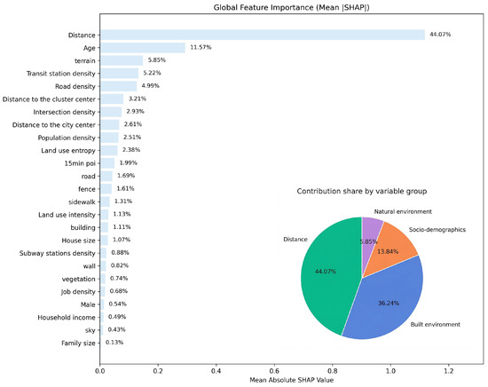
Figure 4. Global feature importance. (Source: Created by the authors).

Compared with distance, built-environment attributes collectively explain 36.24% of the model importance, representing the second major driver of AST behavior. Within this category, macro-scale urban form indicators based on the traditional 5D framework contribute 28.53%, accounting for 78.7% of the built-environment contribution, while micro-scale streetscape attributes derived from street-view imagery account for 7.71% (21.3%). This pattern suggests that, within feasible travel distances, both urban spatial structure and street-level environmental quality jointly shape the accessibility and safety conditions for walking and cycling to school. From a health-related mobility perspective, the strong contribution of school-travel distance and the observed role of built-environment and streetscape variables suggest that children’s daily opportunities for walking or cycling to school are closely tied to both spatial proximity and the quality of the surrounding travel environment.

Socio-demographic attributes contribute relatively modest explanatory power, accounting for 13.84% of the total importance. Notably, age alone accounts for 11.57%, representing 90.9% of the socio-demographic contribution, far exceeding gender, household income, and family size. Given that the sample spans primary to junior-secondary school students, age has clear behavioral implications: As children grow older, their independent mobility increases and parents are more likely to allow them to travel to school independently, thereby increasing the likelihood of active commuting. This relationship has been widely documented in previous studies [37].

An additional noteworthy finding is the prominence of terrain (5.85%), which ranks third in overall importance. Although Wuhan is generally considered a relatively flat city, the results indicate that topographic conditions still exert a measurable influence on children’s active travel behavior. Previous research has demonstrated that steeper slopes increase physical effort for walking or cycling, thereby reducing the likelihood of active school travel [11]. The present findings therefore suggest that terrain may play a more salient role than is often assumed in AST studies.

Examining individual variables further reveals that, following distance and age, the next eight most important variables are predominantly macro-scale 5D built-environment indicators, including transit station density, road density, central accessibility, intersection density, population density, and land-use diversity. These findings indicate that beyond the distance constraint, the presence of a safe, connected, and destination-accessible pedestrian network remains a key structural determinant of active school travel. In contrast, socio-demographic attributes other than age play a comparatively limited role in the overall model importance.

Overall, the results suggest a hierarchical association structure underlying AST: Distance functions as the primary constraint; within feasible travel ranges, built-environment and natural geographic conditions shape the accessibility and safety of active mobility; and individual or household characteristics further moderate these decisions. The following section therefore examines the nonlinear relationships and potential threshold effects between key environmental variables and the probability of active school travel.

3.2. Nonlinearities from Dependence Plots

SHAP dependence plots show how one feature contributes to the model output across its value range. The x-axis is the feature value, and the y-axis is the SHAP value for that feature. Positive SHAP values push the prediction toward a higher likelihood of active school travel, while negative values push it downward. We use scatter points to show heterogeneity, a LOWESS curve to summarize the trend, and bootstrap intervals to highlight stable versus uncertain segments. SHAP is grounded in Shapley-value attribution and was proposed to interpret nonlinear contributions in complex models [34].

Distance is ranked first and contributes 44.07%. The histogram in Figure 5a shows that most school trips are short, but the SHAP value drops sharply as distance increases. The curve crosses zero at approximately 1.3 km of Euclidean home–school distance. This value should be interpreted as a model-indicated transition range in home–school spatial separation, rather than as a precise threshold of actual walking-route distance. The negative effect keeps growing and then stabilizes after roughly 10 km. Distance appears to function as a primary feasibility constraint for AST. Prior evidence consistently identifies distance as the strongest barrier to AST [36,38]. Age ranks second (11.57%). Figure 5b shows negative contributions for ages 6–10. The curve turns positive around ages 10–11 and rises steeply, then increases more slowly. This turning point likely reflects growing independent mobility and higher parental permission. This is consistent with the findings of previous studies. In Canada, older children living within walking distance were more likely to use AST, and parents’ perceived barriers were a strong predictor [37].

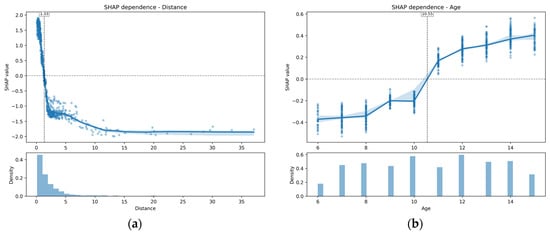
Figure 5. SHAP value plots: nonlinear effects of school-travel distance and age on AST: (a) school-travel distance; (b) age. (Source: Created by the authors).

Among the conventional built-environment variables, transit station density ranks fourth in importance, accounting for 5.22% of the total contribution, and displays a pronounced nonlinear pattern (Figure 6a). Its effect remains negative and relatively stable from about 5 to 32, rises sharply around 33–37, crosses zero, and becomes positive after roughly 40, where it then enters a plateau. At lower and medium levels, higher transit station density is associated with a lower probability of active school travel, whereas at sufficiently high levels the association turns positive. A cautious interpretation is that low-to-medium transit density may be linked to traffic-intensive corridor environments or to contexts in which public transport provides an alternative to walking and cycling, while very high transit density may better reflect compact and service-rich urban settings with stronger overall accessibility. Prior studies have likewise noted that public transport environments can be related to school travel behavior in complex ways rather than through a single monotonic effect [39].

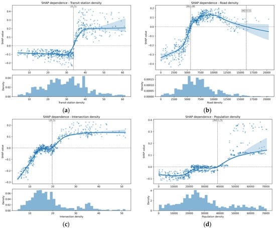
Figure 6. SHAP value plots: nonlinear effects of conventional built-environment variables on AST: (a) transit station density; (b) road density; (c) intersection density; (d) population density. (Source: Created by the authors).

Road density ranks fifth (4.99%) and follows an inverted-U pattern (Figure 6b). Below ~5000 m/km², contributions are clearly negative. The curve crosses zero around ~5000–6000 m/km² and rises quickly. It peaks around ~8000–10,000 m/km². The effect then weakens and approaches zero again near ~15,000 m/km². This pattern may indicate that the accessibility benefits of denser road networks are partly offset by greater traffic exposure or crossing complexity in some ranges. Sparse networks imply detours and limited walking/cycling options. Moderate networks improve directness and route choice. Very dense road systems often co-occur with higher traffic exposure, which can erode benefits for children. Route-based evidence supports this view. Neighborhood, route, and school environments jointly shape school travel, and distance moderates these associations [11].

Intersection density ranks seventh (2.93%). It increases and then plateaus (Figure 6c). The contribution is near zero at about 15–20. It turns clearly positive above 20 and levels off at around 30. This suggests higher marginal gains in low-connectivity areas and diminishing returns in already connected areas. The direction aligns with prior synthesis. An individual-participant meta-analysis found a positive association between intersection density and AST, while distance remained the strongest predictor [25].

Population density ranks ninth (2.51%) and shows a segmented pattern (Figure 6d). Contributions are negative below ~10 k, close to zero around ~20–30 k, and positive above ~40 k. Low density often implies sparse destinations and weak street activity, which makes AST less feasible. Higher density can support services and walking activity and thus supports AST. Prior evidence is mixed on the sign of density. In New Zealand, dwelling density was negatively associated with AST in an IPD meta-analysis [25]. This indicates that its effect operates within a range rather than a single linear relationship.

The centrality variables further reveal spatial differentiation in the active school travel environment. Distance to the cluster center accounts for 3.21% (Rank: 6) of total importance, slightly higher than distance to the city center at 2.61% (Rank: 8). Figure 7a shows a clear inverted-U relationship for distance to the cluster center. The effect is generally negative within about 0–2 km, turns positive in the 2–4 km range, reaches a peak at around 3–3.5 km, and then declines sharply after 4.2 km, becoming negative again. In contrast, Figure 7b shows a more continuous decay pattern for distance to the city center. The effect remains positive within about 0–4.5 km, but weakens steadily with increasing distance, crosses zero at around 5 km, and becomes stably negative after roughly 10 km. These two patterns suggest that the centrality effects of the main center and cluster centers are not the same. For the main center, proximity is generally associated with a higher propensity for active school travel, although this advantage gradually weakens with distance. For cluster centers, the nearest zone does not show a positive effect; instead, the most favorable pattern appears in the middle-distance range. Together, these results indicate that urban centrality does not influence children’s active school travel in a simple linear way, but shows clear differences across spatial scales.

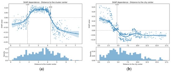
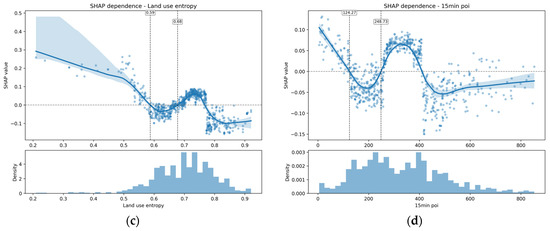
Figure 7. SHAP value plots: nonlinear effects of centrality and land-use-related variables on AST: (a) distance to the cluster center; (b) distance to the city center; (c) land-use entropy; (d) 15 min POI density. (Source: Created by the authors).

Land-use entropy ranks tenth (2.38%) and shows multi-stage fluctuations (Figure 7c). Values around 0.2–0.5 are positive but declining. The curve crosses zero near ~0.58 and reaches a negative trough around ~0.60–0.64. It rises again with a local peak around ~0.70–0.76, then turns negative after ~0.78 and stays negative around ~0.82–0.90. Moderate mix can reduce travel distances and improve accessibility. Very high mix can also imply heavier flows and more curbside complexity, which may increase perceived risk. Reviews show that relationships of density, diversity, and design with AST vary across contexts [15].

Fifteen min POI density ranks eleventh (1.99%) and shows multiple peaks and troughs (Figure 7d). The effect declines from ~100 to ~200 and reaches a trough near ~200. It becomes positive with a peak around ~300–380. It turns negative again around ~400–500, then gradually returns toward zero. This indicates an effective range for support service density. Very low POI density often reflects low convenience and weak walking activity in peripheral areas. Moderate density can improve route legibility and provide supportive nodes. Excessive density may bring more curbside activity and traffic conflicts. In Hong Kong, transit facilities and leisure venues were significant correlates of children’s AST, and the interpretation depends on pedestrian networks and crossings [40].

At the micro scale, natural and streetscape variables add mechanisms that macro indicators may miss. Terrain is particularly salient. It ranks third and contributes 5.85% (Figure 8a). The effect is positive at very low values but weakens with increasing terrain. It crosses zero near ~0.027 and becomes negative. It then plateaus after ~0.03. Even modest slope can reduce acceptable walking and cycling ranges through physical effort, cycling stability, and perceived risk. Route-based evidence shows steep slopes increase parental safety concerns, while higher intersection density and tree canopy can mitigate them [41]. In a mountainous Chinese city, slope strongly deters AST for suburban students with longer trips [42].

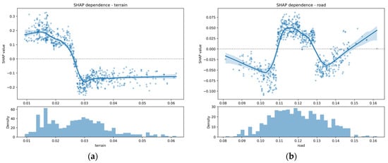
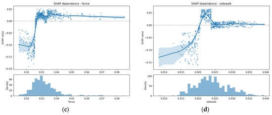
Figure 8. SHAP value plots: nonlinear effects of terrain and micro-scale streetscape variables on AST: (a) terrain; (b) roadway share; (c) fence share; (d) sidewalk share. (Source: Created by the authors).

Road (1.69%), fence (1.61%), and sidewalk (1.31%) are less important than terrain, but they still show threshold or multi-stage patterns (Figure 8b–d). The W-shaped road curve suggests changing meanings across ranges. Fence turns from negative to positive around ~0.027 and then plateaus. Sidewalk turns positive near ~0.02, peaks around ~0.023, and then flattens after ~0.025, suggesting that benefits come from meeting a minimum standard of continuity and safety. Streetscape evidence also shows that higher pavement ratios can be linked to lower odds of AST in some contexts [21], and reviews stress that perceived traffic safety can be improved through lateral separation measures [43].

3.3. Interaction Effects on AST

To further identify whether the association of one variable with AST depends on the level of another variable, SHAP interaction values were computed for all pairwise combinations of predictors. For each variable pair, the mean absolute interaction value across the test sample was calculated and used to rank interaction strength. To improve the transparency of the interaction analysis, the top ten pairwise SHAP interactions are reported in Table 5. Among these ranked pairs, six interactions were selected for 3D visualization and discussion because they showed both relatively high interaction strength and clearer interpretable surface patterns. These selected pairs were then visualized as smoothed 3D interaction surfaces, where the two horizontal axes represent the values of the paired variables and the vertical axis represents the corresponding SHAP interaction contribution. This procedure helps move beyond single-variable dependence patterns and shows how the association of one predictor with AST varies across the value range of another predictor. The behavioral interpretations in this section should be understood as plausible explanations of the model patterns, since parental escort, safety perception, and household decision-making variables were not directly measured.

Table 5. Top ten SHAP interaction pairs.

Rank	Interaction Pair	Mean Absolute SHAP Interaction Value
1	Age × Distance	0.0420
2	Transit station density × Distance	0.0335
3	Population density × Distance	0.0310
4	Distance to the city center × Distance	0.0295
5	Distance × Terrain	0.0281
6	Age × Terrain	0.0157
7	Road density × Age	0.0155
8	Intersection density × Distance	0.0143
9	15 min POI density × Distance	0.0135
10	Road density × Transit station density	0.0128

(Source: Created by the authors).

Top1 (Age × Distance) shows a particularly clear joint age–distance pattern (Figure 9). Within short-distance ranges, older age is generally associated with a more favorable AST combination. This is consistent with the single-variable result, where the age effect turns from negative to positive at around 10–11 years. A different pattern appears once school-travel distance exceeds about 1.3 km. In this range, the interaction surface suggests that, in some segments, children aged 6–8 show a higher AST propensity than those aged 10–14. This does not contradict the positive main effect of age. Rather, it suggests that the age effect is reorganized once distance becomes more restrictive.

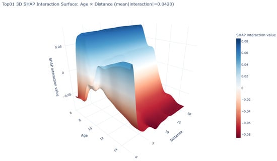
Figure 9. Interactive effects of age and school-travel distance on AST. (Source: Created by the authors).

One possible interpretation is that AST may reflect both children’s mobility capacity and household travel decisions, rather than only individual preference for walking or cycling. The first step involves determining whether accompaniment is necessary, followed by selecting the mode of school travel [44]. Previous studies show that older children are more likely to commute without an adult escort, whereas parental escort declines with age [45]. For older students, moderate travel distances are associated with both a larger activity space and a broader choice set. This makes them more likely to shift from walking or cycling to public transport or other more efficient non-active modes. Existing research also suggests that distance is not only the primary constraint on AST, but is also an important factor in the balance between active travel and public transport; as distance increases, public transport generally becomes more attractive [39]. By contrast, younger children also show declining AST propensity in this distance band, but the decline is less pronounced than that of older students. This produces a relatively higher local tendency in the interaction surface. The key point is not that younger children generally prefer active travel over longer distances. Rather, older students appear to shift out of walking or cycling more quickly once the main distance threshold is crossed.

Overall, the Age × Distance interaction does not simply amplify the positive main effect of age. Instead, it shows that age operates differently across distance bands. Under short-distance conditions, increasing age mainly reflects greater independent mobility. Once the key distance threshold is exceeded, however, increasing age also implies a greater likelihood of mode substitution. This distance-contingent age effect cannot be fully captured by single-variable analysis alone.

Top2 (Transit station density × Distance) shows that higher transit station density is associated with lower AST propensity at short distances, but this negative association weakens and turns positive at longer distances (Figure 10). The interaction surface changes clearly around the model-indicated transition range of about 1.3 km. At short distances, low stop density shows only a weak positive interaction, but the interaction rapidly turns negative as stop density increases, showing a stronger negative interaction around 40. This suggests that, within trips that are already feasible for walking or cycling, high transit supply does not reinforce AST. Instead, it is associated with a lower propensity for walking or cycling.

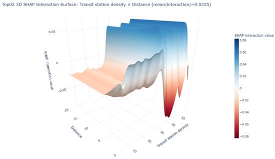
Figure 10. Interactive effects of transit station density and school-travel distance on AST. (Source: Created by the authors).

The surface pattern indicates that distance changes the behavioral meaning of stop density. When a school is close, sparse stop provision does not create a strong substitute, so walking and cycling remain the most direct options. Once stop density becomes high, however, substitute modes become easier to access. At the same time, high-stop-density areas often involve heavier traffic activity and stronger curbside friction. The pedestrian environment is therefore not necessarily more favorable, and AST is associated with a lower predicted propensity.

At longer distances, the interaction pattern becomes broadly consistent with the single-variable dependence plot, with values below 40 remaining suppressive and values above 40 gradually turning supportive. This shift suggests that, beyond this distance-related transition range, stop density is no longer only a competing travel option. It also reflects broader accessibility, functional concentration, and network connectivity. Loh et al. [39] report a similar pattern, showing that distance moderates how built-environment variables relate to both active travel and public transport use.

Top3 (Population density × Distance) shows that high population density has limited additional association with AST for very short trips but becomes more positively associated with AST as school-travel distance increases (Figure 11). Specifically, the interaction surface shows a modest negative interaction in the high-density and short-distance range. As distance increases, however, the interaction quickly turns positive, and the buffering role of high density against distance becomes much stronger. By contrast, the surface remains relatively flat in low-density areas, suggesting that in more dispersed environments density does little to alter the dominant role of distance.

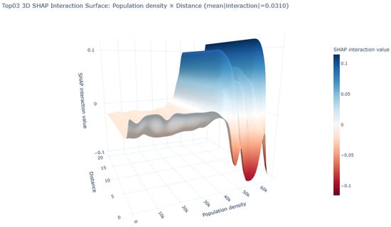
Figure 11. Interactive effects of population density and school-travel distance on AST. (Source: Created by the authors).

Compared with the single-variable result, the key new point is that the positive role of population density does not operate equally across all distance bands. For very short school trips, distance already provides a strong accessibility advantage, and the compactness benefit of dense environments may already be absorbed by the main effects. Additional pedestrian and traffic intensity may then reduce the interaction gain. Once distance enters a range in which households must weigh alternatives, however, the advantages of high density become more visible. Dense environments usually imply shorter school service radii, more continuous route networks, and stronger destination concentration, all of which help offset the distance penalty.

Therefore, the Population density × Distance interaction does not mean that higher density always increases AST. Instead, it suggests that the association between density and AST is contingent on school-travel distance.

Top4 (Distance to the city center × Distance) shows a clear interaction between distance to the city center and school-travel distance (Figure 12). Within the short-distance range, being closer to the city center is associated with a stronger negative interaction, whereas being farther from the center shows a weak positive interaction. In other words, when a school is already close a central location does not further increase AST propensity and may even weaken it. Once school distance exceeds about 1.3 km, the surface begins to resemble the single-variable dependence pattern: being closer to the city center becomes generally favorable to AST, although this advantage gradually weakens and turns slightly negative after about 4–5 km.

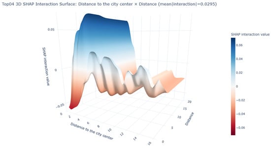
Figure 12. Interactive effects of distance to the city center and school-travel distance on AST. (Source: Created by the authors).

This result suggests that the effect of distance to the city center is not the same across school-distance ranges. For very short trips, the accessibility advantage of central areas may be offset by a more complex traffic environment. As a result, being closer to the center does not necessarily support walking or cycling. When school distance becomes longer, however, the compact urban structure, higher service density, and better network connectivity of central areas begin to matter more. These features can partly offset the negative effect of longer travel distance. Therefore, this interaction does not suggest that proximity to the city center always promotes or suppresses AST. Rather, a part of its effect is conditioned by the school-distance range.

Top6 (Age × terrain) is the first leading interaction term that does not include distance, suggesting that children’s age and terrain jointly affect active school travel beyond the dominant role of distance (Figure 13). The interaction surface shows a clear reversal pattern. Under lower terrain conditions, younger children tend to have more positive interaction values with terrain. As terrain increases, this pattern gradually reverses: Older children show stronger positive interaction values, while younger children are more likely to show negative values. In other words, gentle terrain appears to be more compatible with active school travel among younger children, whereas age-related differences become more evident as terrain becomes more challenging.

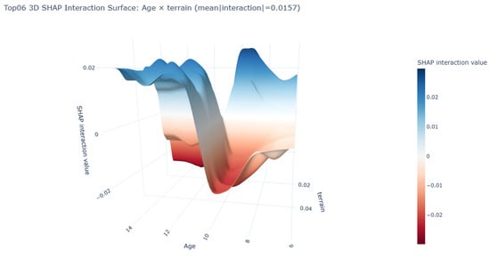
Figure 13. Interactive effects of age and terrain on AST. (Source: Created by the authors).

This may be because, under low-slope conditions, topographic barriers are weak, so age-related advantages in physical capacity and independent mobility are less apparent. When slope increases, however, the physical burden and route complexity of the school trip also increase, making the advantages of older children more visible. This interpretation is broadly consistent with previous studies. Timperio et al. [13] found that, among younger children, a steep incline along the route to school was negatively associated with walking or cycling to school.

Top7 (road density × Age) also shows clear age-related heterogeneity (Figure 14). Children under 10 exhibit positive interaction effects only in low-road-density areas, and the interaction value quickly falls back to around zero as road density increases. In contrast, after about age 11, the surface increasingly resembles the main effect shown in the road density dependence plot: Low road density is associated with negative interaction values, the effect turns positive at around 5600, and the positive interaction then gradually weakens as road density continues to rise. This pattern suggests that the effect of road density is not uniform across age groups; both its direction and strength vary with age.

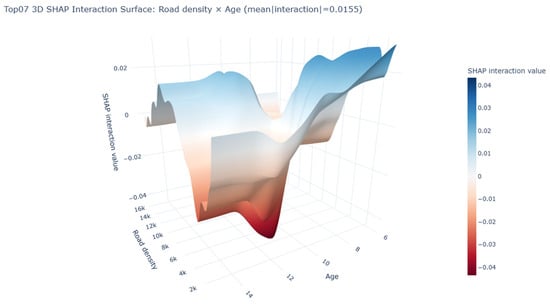
Figure 14. Interactive effects of road density and age on AST. (Source: Created by the authors).

A plausible explanation is that younger children do not respond to road density simply through the usual “denser networks promote active school travel” mechanism. Their behavior is more likely to be constrained by limited independent mobility and stronger parental safety concerns. Marzi et al. [46] reviewed evidence showing that younger children generally have lower levels of independent mobility. Under this logic, low-road-density areas may still support active school travel among younger children because the traffic setting is often simpler and crossing demands are lower, making accompanied walking more acceptable to parents. As road density increases, however, better connectivity is accompanied by more intersections, more complex crossing tasks, and higher perceived traffic exposure, which may offset the benefits of improved accessibility for younger children [17]. For older children, especially those in secondary school, higher independent mobility and better route judgment allow them to benefit more directly from the accessibility gains of denser street networks, leading to a nonlinear pattern that is closer to the main effect.

4. Discussion

Based on the above findings, this study suggests that children’s active school travel is not linearly driven by any single factor. Instead, it is associated with multiple domains, including school-travel distance, the built environment, socio-demographic characteristics, and the natural environment. Existing reviews likewise show that AST is embedded in individual, family, environmental, and external conditions, while many previous studies still treat environmental variables as homogeneous and linear effects [10,11,15,47]. Using XGBoost–SHAP, this study further shows that the association structure of AST is hierarchical, nonlinear, and condition-dependent. Distance remains the dominant contributor, while the overall contribution of the built environment is about three times that of socio-demographic attributes; terrain also shows a non-negligible role. Accordingly, children’s school travel should not be reduced to a simple proposition that shorter distance always promotes AST or that more compact environments are always more supportive. A more accurate reading is that AST emerges under a basic feasibility constraint and is jointly associated with multiple spatial conditions. The value of this study therefore lies not only in identifying what matters more, but also in revealing conditional association patterns that are easily obscured by average-effect frameworks.

In this distance-driven context, the built environment variables exhibit a clearly nonlinear relationship with AST. Transit station density, road density, intersection density, population density, land-use mix, and facility density all vary in both direction and strength across value ranges. This is consistent with recent reviews showing that environmental correlates of AST are often mixed and highly context-dependent [10,15]. In practical terms, greater connectivity, walkability, or accessibility may shorten detours and enrich route choice, but higher density, stronger clustering of activities, and richer transport supply may also increase traffic exposure, crossing conflicts, or substitution toward non-active modes. Existing empirical work reports similar mixed evidence: some studies find positive associations of intersection density, walkability, or school siting conditions with AST, while others show that the effects of density, traffic exposure, or neighborhood characteristics are not stable and may even differ between the trip to school and the trip from school [16,18,19,48]. In this sense, the staged and sometimes reversing patterns observed here for transit station density, road density, land-use entropy, and 15 min POI density are not isolated findings. Rather, these findings support the notion that the attributes of the built environment may play different roles depending on their intensity.

It is also important that the present analysis includes not only macro-scale indicators of urban structure, such as distance to the city center and distance to the cluster center, but also finer-scale environmental features, including streetscape and terrain. One notable finding is that distance to the cluster center contributes slightly more than distance to the city center, and shows a clear inverted-U relationship with AST. By contrast, distance to the city center is closer to a monotonic declining pattern. A more cautious interpretation is that, in a multi-centered city such as Wuhan, different levels of centrality may imply different school-travel environments for children. Greater proximity to the main center may imply stronger overall accessibility, but also greater traffic complexity, whereas an intermediate distance from local clusters may combine relatively good local service accessibility with more manageable traffic pressure. At the same time, the relatively high importance of terrain suggests that AST studies omitting topography may underestimate the role of route burden and physical effort. This point has received preliminary support in studies of hilly and mountainous cities, including recent evidence from China [42,49].

The interaction results further show that children should not be treated as a homogeneous group. The same environmental condition does not carry the same meaning across age groups or distance contexts. Distance is not only the most important variable in the model, but also interacts with several other variables, with the overall pattern shifting around approximately 1.3 km. This suggests that treating distance as an ordinary control variable may underestimate its role in amplifying or attenuating the associations of other variables [11,50]. Age shows a similar pattern. Around age 11, the interactions of age with terrain and road density change clearly in direction and strength. This indicates that some built-environment variables may appear weak or unstable in the full sample not because they are unimportant, but because their associations only emerge within specific age groups or distance bands. The interaction patterns reported here therefore represent more than a statistical result. They make visible the internal heterogeneity of children’s school-travel decisions. Studies relying only on pooled regression coefficients or single main effects are likely to average away this heterogeneity and miss the most targeted planning implications [51]. These findings also have health-related planning implications. Since AST is a routine source of children’s daily physical activity, built-environment conditions associated with higher AST propensity may help create more health-supportive school-travel environments [52]. In addition to improving physical walking and cycling conditions, road-safety education and safety-related interventions are also important for supporting children’s participation in active travel [53].

As a large, multi-centered Chinese city, Wuhan provides a useful case for examining children’s AST in rapidly urbanizing metropolitan contexts. However, associations involving transit density, population density, and centrality may vary across urban forms and transport systems. Therefore, the findings should be interpreted as context-specific evidence that may be most transferable to large cities with similar multi-centered spatial structures and heterogeneous built environments.

Overall, this study offers a more conditional perspective for AST research. Rather than remaining at the level of asking whether the built environment is associated with AST in general, future work should move toward asking under what conditions, for which groups of children, and through what combinations of factors the built environment is associated with AST. This shift implies a deeper explanation and also a change in methods and planning logic. For practice, promoting AST should not rely on a universal spatial optimization logic. More differentiated strategies are needed by age, distance, and context. For younger children, shortening actual school-travel distance, reducing route complexity, and improving crossing safety may matter more than simply increasing land-use mix. For older children, the key question may be which environmental conditions can maintain the feasibility of active travel under somewhat longer distances or more complex street networks. However, such patterns should be interpreted as conditional associations identified by the model, rather than as the direct causal effects of the built environment on children’s travel behavior. Even so, the present findings still show that the association structure of children’s AST is more complex than traditional frameworks suggest, and making this complexity visible is itself a methodological contribution.

5. Conclusions

This study applied the XGBoost–SHAP framework to examine the associations of school-travel distance, the built environment, socio-demographic attributes, and the natural environment with children’s AST. The results show that AST is characterized by clear hierarchy, nonlinearity, and conditional dependence. Distance remains the most important correlate. The overall explanatory contribution of the built environment is much higher than that of socio-demographic attributes, while terrain and other natural factors also play a non-negligible role. In addition, built-environment variables show clear range differences and directional shifts. Distance and age also condition the strength of the associations between other environmental factors and AST, suggesting that children should not be treated as a homogeneous group. Overall, this study suggests that AST research should move beyond full-sample main-effect identification and pay more attention to age- and distance-stratified mechanisms. These findings also imply that child-friendly school-travel planning should shift from general environmental optimization toward more targeted strategies across age, distance, and context. Although this study focuses on AST behavior rather than direct health outcomes, the findings highlight the importance of built-environment conditions for supporting health-related daily mobility among children.

Several limitations should be noted. The dataset does not include school-level characteristics, parental escort behavior, parental safety perceptions, or other household decision-making variables. In addition, this study is based on observational cross-sectional data; therefore, the results should be interpreted as associations rather than causal effects. The nonlinear patterns and interaction structures identified by SHAP are model-based interpretations, and the observed transition ranges should not be treated as statistically tested thresholds or direct behavioral mechanisms. Future studies could compare different types of cities to further examine the transferability of these findings.

References

- Bull, F.C.; Al-Ansari, S.S.; Biddle, S.; Borodulin, K.; Buman, M.P.; Cardon, G.; Carty, C.; Chaput, J.-P.; Chastin, S.; Chou, R.; et al. World Health Organization 2020 Guidelines on Physical Activity and Sedentary Behaviour. Br. J. Sports Med. 2020, 54, 1451–1462. [Google Scholar] [CrossRef] [PubMed]
- Chaput, J.-P.; Willumsen, J.; Bull, F.; Chou, R.; Ekelund, U.; Firth, J.; Jago, R.; Ortega, F.B.; Katzmarzyk, P.T. 2020 WHO Guidelines on Physical Activity and Sedentary Behaviour for Children and Adolescents Aged 5–17 Years: Summary of the Evidence. Int. J. Behav. Nutr. Phys. Act. 2020, 17, 141. [Google Scholar] [CrossRef] [PubMed]
- Faulkner, G.E.J.; Buliung, R.N.; Flora, P.K.; Fusco, C. Active School Transport, Physical Activity Levels and Body Weight of Children and Youth: A Systematic Review. Prev. Med. 2009, 48, 3–8. [Google Scholar] [CrossRef]
- Lubans, D.R.; Boreham, C.A.; Kelly, P.; Foster, C.E. The Relationship between Active Travel to School and Health-Related Fitness in Children and Adolescents: A Systematic Review. Int. J. Behav. Nutr. Phys. Act. 2011, 8, 5. [Google Scholar] [CrossRef]
- Schoeppe, S.; Duncan, M.J.; Badland, H.; Oliver, M.; Curtis, C. Associations of Children’s Independent Mobility and Active Travel with Physical Activity, Sedentary Behaviour and Weight Status: A Systematic Review. J. Sci. Med. Sport 2013, 16, 312–319. [Google Scholar] [CrossRef]
- Desjardins, E.; Tavakoli, Z.; Páez, A.; Waygood, E.O.D. Children’s Access to Non-School Destinations by Active or Independent Travel: A Scoping Review. Int. J. Environ. Res. Public Health 2022, 19, 12345. [Google Scholar] [CrossRef]
- McDonald, N.C. Active Transportation to School: Trends Among U.S. Schoolchildren, 1969–2001. Am. J. Prev. Med. 2007, 32, 509–516. [Google Scholar] [CrossRef]
- Yang, Y.; Xue, H.; Liu, S.; Wang, Y. Is the Decline of Active Travel to School Unavoidable By-Products of Economic Growth and Urbanization in Developing Countries? Sustain. Cities Soc. 2019, 47, 101446. [Google Scholar] [CrossRef]
- Yang, Y.; Hong, X.; Gurney, J.G.; Wang, Y. Active Travel to and from School Among School-Age Children During 1997–2011 and Associated Factors in China. J. Phys. Act. Health 2017, 14, 684–691. [Google Scholar] [CrossRef] [PubMed]
- Lam, H.Y.; Jayasinghe, S.; Ahuja, K.D.K.; Hills, A.P. Active School Commuting in School Children: A Narrative Review of Current Evidence and Future Research Implications. Int. J. Environ. Res. Public Health 2023, 20, 6929. [Google Scholar] [CrossRef]
- Panter, J.R.; Jones, A.P.; Sluijs, E.M.F.V.; Griffin, S.J. Neighborhood, Route, and School Environments and Children’s Active Commuting. Am. J. Prev. Med. 2010, 38, 268–278. [Google Scholar] [CrossRef]
- Panter, J.R.; Jones, A.P.; van Sluijs, E.M. Environmental Determinants of Active Travel in Youth: A Review and Framework for Future Research. Int. J. Behav. Nutr. Phys. Act. 2008, 5, 34. [Google Scholar] [CrossRef]
- Timperio, A.; Ball, K.; Salmon, J.; Roberts, R.; Giles-Corti, B.; Simmons, D.; Baur, L.A.; Crawford, D. Personal, Family, Social, and Environmental Correlates of Active Commuting to School. Am. J. Prev. Med. 2006, 30, 45–51. [Google Scholar] [CrossRef]
- Galán, A.; Ruiz-Apilánez, B.; Macdonald, E. Built Environment and Active Transportation to School in the West: Latest Evidence and Research Methods. Discov. Cities 2024, 1, 3. [Google Scholar] [CrossRef]
- D’Haese, S.; Vanwolleghem, G.; Hinckson, E.; De Bourdeaudhuij, I.; Deforche, B.; Van Dyck, D.; Cardon, G. Cross-Continental Comparison of the Association between the Physical Environment and Active Transportation in Children: A Systematic Review. Int. J. Behav. Nutr. Phys. Act. 2015, 12, 145. [Google Scholar] [CrossRef]
- Bosch, L.S.M.M.; Wells, J.C.K.; Lum, S.; Reid, A.M. Associations of the objective built environment along the route to school with children’s modes of commuting: A multilevel modelling analysis (the SLIC study). PLoS ONE 2020, 15, e0231478. [Google Scholar] [CrossRef] [PubMed]
- Giles-Corti, B.; Wood, G.; Pikora, T.; Learnihan, V.; Bulsara, M.; Van Niel, K.; Timperio, A.; McCormack, G.; Villanueva, K. School Site and the Potential to Walk to School: The Impact of Street Connectivity and Traffic Exposure in School Neighborhoods. Health Place 2011, 17, 545–550. [Google Scholar] [CrossRef] [PubMed]
- Larsen, K.; Gilliland, J.; Hess, P.; Tucker, P.; Irwin, J.; He, M. The Influence of the Physical Environment and Sociodemographic Characteristics on Children’s Mode of Travel to and from School. Am. J. Public Health 2009, 99, 520–526. [Google Scholar] [CrossRef]
- Aarts, M.-J.; Mathijssen, J.J.P.; van Oers, J.A.M.; Schuit, A.J. Associations between Environmental Characteristics and Active Commuting to School Among Children: A Cross-Sectional Study. Int. J. Behav. Med. 2013, 20, 538–555. [Google Scholar] [CrossRef]
- Wang, X.; Liu, Y.; Zhu, C.; Yao, Y.; Helbich, M. Associations between the Streetscape Built Environment and Walking to School Among Primary Schoolchildren in Beijing, China. J. Transp. Geogr. 2022, 99, 103303. [Google Scholar] [CrossRef]
- Wang, X.; Liu, Y.; Yao, Y.; Zhou, S.; Zhu, Q.; Liu, M.; Helbich, M. Adolescents’ Environmental Perceptions Mediate Associations between Streetscape Environments and Active School Travel. Transp. Res. Part D Transp. Environ. 2023, 114, 103549. [Google Scholar] [CrossRef]
- Kang, Y.; Zhang, F.; Gao, S.; Lin, H.; Liu, Y. A Review of Urban Physical Environment Sensing Using Street View Imagery in Public Health Studies. Ann. GIS 2020, 26, 261–275. [Google Scholar] [CrossRef]
- Yang, Y.; Lu, Y.; Yang, L.; Gou, Z.; Zhang, X. Urban Greenery, Active School Transport, and Body Weight Among Hong Kong Children. Travel Behav. Soc. 2020, 20, 104–113. [Google Scholar] [CrossRef]
- Wu, F.; Li, W.; Qiu, W. Examining Non-Linear Relationship between Streetscape Features and Propensity of Walking to School in Hong Kong Using Machine Learning Techniques. J. Transp. Geogr. 2023, 113, 103698. [Google Scholar] [CrossRef]
- Ikeda, E.; Stewart, T.; Garrett, N.; Egli, V.; Mandic, S.; Hosking, J.; Witten, K.; Hawley, G.; Tautolo, E.S.; Rodda, J.; et al. Built Environment Associates of Active School Travel in New Zealand Children and Youth: A Systematic Meta-Analysis Using Individual Participant Data. J. Transp. Health 2018, 9, 117–131. [Google Scholar] [CrossRef]
- Tang, R.; Shi, Z.; He, M.; Min, S.; Liu, Y. Determinants of Active School Travel Levels Among Children: A Case Study in a Mountainous City. J. Transp. Health 2025, 44, 102099. [Google Scholar] [CrossRef]
- Yang, S.; Zhou, L.; Liu, C.; Sun, S.; Guo, L.; Sun, X. Examining Multiscale Built Environment Interventions to Mitigate Travel-Related Carbon Emissions. J. Transp. Geogr. 2024, 119, 103942. [Google Scholar] [CrossRef]
- Chica-Olmo, J.; Rodríguez-López, C.; Chillón, P. Effect of Distance from Home to School and Spatial Dependence between Homes on Mode of Commuting to School. J. Transp. Geogr. 2018, 72, 1–12. [Google Scholar] [CrossRef]
- Liu, Y.; Zhang, Y.; Jin, S.T.; Liu, Y. Spatial Pattern of Leisure Activities Among Residents in Beijing, China: Exploring the Impacts of Urban Environment. Sustain. Cities Soc. 2020, 52, 101806. [Google Scholar] [CrossRef]
- Guo, L.; Zheng, C.; Huang, J.; Yuan, M.; Ma, Y.; He, H. Commuting Circle-Based Spatial Structure Optimization of Megacities: A Case Study of Wuhan Central City. City Plan. Rev. 2019, 43, 43–54. [Google Scholar]
- He, H.; Zhou, L.; Yang, S.; Guo, L. Why Choose Active Travel over Driving? Investigating the Impact of the Streetscape and Land Use on Active Travel in Short Journeys. J. Transp. Geogr. 2024, 118, 103939. [Google Scholar] [CrossRef]
- O’brien, R.M. A Caution Regarding Rules of Thumb for Variance Inflation Factors. Qual. Quant. 2007, 41, 673–690. [Google Scholar] [CrossRef]
- Chen, T.; Guestrin, C. XGBoost: A Scalable Tree Boosting System. In Proceedings of the 22nd ACM SIGKDD International Conference on Knowledge Discovery and Data Mining; Association for Computing Machinery: New York, NY, USA, 2016; pp. 785–794. [Google Scholar]
- Lundberg, S.M.; Lee, S.-I. A Unified Approach to Interpreting Model Predictions. In Proceedings of the Advances in Neural Information Processing Systems 30 (NIPS 2017); Guyon, I., Luxburg, U.V., Bengio, S., Wallach, H., Fergus, R., Vishwanathan, S., Garnett, R., Eds.; Neural Information Processing Systems (NIPS): La Jolla, CA, USA, 2017; Volume 30. [Google Scholar]
- Mitra, R.; Buliung, R.N. Built Environment Correlates of Active School Transportation: Neighborhood and the Modifiable Areal Unit Problem. J. Transp. Geogr. 2012, 20, 51–61. [Google Scholar] [CrossRef]
- Rothman, L.; Macpherson, A.K.; Ross, T.; Buliung, R.N. The Decline in Active School Transportation (AST): A Systematic Review of the Factors Related to AST and Changes in School Transport over Time in North America. Prev. Med. 2018, 111, 314–322. [Google Scholar] [CrossRef] [PubMed]
- Wilson, K.; Clark, A.F.; Gilliland, J.A. Understanding Child and Parent Perceptions of Barriers Influencing Children’s Active School Travel. BMC Public Health 2018, 18, 1053. [Google Scholar] [CrossRef]
- Macdonald, L.; McCrorie, P.; Nicholls, N.; Olsen, J.R. Active Commute to School: Does Distance from School or Walkability of the Home Neighbourhood Matter? A National Cross-Sectional Study of Children Aged 10–11 Years, Scotland, UK. BMJ Open 2019, 9, e033628. [Google Scholar] [CrossRef]
- Loh, V.; Sahlqvist, S.; Veitch, J.; Walsh, A.; Cerin, E.; Salmon, J.; Mavoa, S.; Timperio, A. Active Travel, Public Transport and the Built Environment in Youth: Interactions with Perceived Safety, Distance to School, Age and Gender. J. Transp. Health 2024, 38, 101895. [Google Scholar] [CrossRef]
- Leung, K.Y.K.; Loo, B.P.Y. Determinants of Children’s Active Travel to School: A Case Study in Hong Kong. Travel Behav. Soc. 2020, 21, 79–89. [Google Scholar] [CrossRef]
- Kim, Y.-J.; Lee, C. Built and Natural Environmental Correlates of Parental Safety Concerns for Children’s Active Travel to School. Int. J. Environ. Res. Public Health 2020, 17, 517. [Google Scholar] [CrossRef]
- Liu, Y.; Min, S.; Shi, Z.; He, M. Exploring Students’ Choice of Active Travel to School in Different Spatial Environments: A Case Study in a Mountain City. J. Transp. Geogr. 2024, 115, 103795. [Google Scholar] [CrossRef]
- Wangzom, D.; White, M.; Paay, J. Perceived Safety Influencing Active Travel to School—A Built Environment Perspective. Int. J. Environ. Res. Public Health 2023, 20, 1026. [Google Scholar] [CrossRef]
- Faulkner, G.E.; Richichi, V.; Buliung, R.N.; Fusco, C.; Moola, F. What’s “Quickest and Easiest?”: Parental Decision Making about School Trip Mode. Int. J. Behav. Nutr. Phys. Act. 2010, 7, 62. [Google Scholar] [CrossRef]
- Carver, A.; Panter, J.R.; Jones, A.P.; van Sluijs, E.M.F. Independent Mobility on the Journey to School: A Joint Cross-Sectional and Prospective Exploration of Social and Physical Environmental Influences. J. Transp. Health 2014, 1, 25–32. [Google Scholar] [CrossRef]
- Marzi, I.; Reimers, A.K. Children’s Independent Mobility: Current Knowledge, Future Directions, and Public Health Implications. Int. J. Environ. Res. Public Health 2018, 15, 2441. [Google Scholar] [CrossRef]
- Ginja, S.; Arnott, B.; Namdeo, A.; McColl, E. Understanding Active School Travel through the Behavioural Ecological Model. Health Psychol. Rev. 2018, 12, 58–74. [Google Scholar] [CrossRef]
- Hino, K.; Ikeda, E.; Sadahiro, S.; Inoue, S. Associations of Neighborhood Built, Safety, and Social Environment with Walking to and from School Among Elementary School-Aged Children in Chiba, Japan. Int. J. Behav. Nutr. Phys. Act. 2021, 18, 152. [Google Scholar] [CrossRef] [PubMed]
- Müller, S.; Mejia-Dorantes, L.; Kersten, E. Analysis of Active School Transportation in Hilly Urban Environments: A Case Study of Dresden. J. Transp. Geogr. 2020, 88, 102872. [Google Scholar] [CrossRef]
- Ross, A.; Godwyll, J.; Adams, M. The Moderating Effect of Distance on Features of the Built Environment and Active School Transport. Int. J. Environ. Res. Public Health 2020, 17, 7856. [Google Scholar] [CrossRef]
- Molina-García, J.; García-Massó, X.; Sallis, J.F.; Queralt, A. Built Environment and Active Commuting to School: The Moderating Effects of Psychosocial Factors and Neighborhood Safety in Girls and Boys. J. Transp. Health 2025, 45, 102187. [Google Scholar] [CrossRef]
- Fitch-Polse, D.; Agarwal, S. The Benefits of Active Transportation Interventions: A Review of the Evidence. J. Transp. Land Use 2025, 18, 77–122. [Google Scholar] [CrossRef]
- Buttazzoni, A.; Pham, J.; Nelson Ferguson, K.; Fabri, E.; Clark, A.; Tobin, D.; Frisbee, N.; Gilliland, J. Supporting Children’s Participation in Active Travel: Developing an Online Road Safety Intervention through a Collaborative Integrated Knowledge Translation Approach. Int. J. Qual. Stud. Health Well-Being 2024, 19, 2320183. [Google Scholar] [CrossRef] [PubMed]
Disclaimer/Publisher’s Note: The statements, opinions and data contained in all publications are solely those of the individual author(s) and contributor(s) and not of MDPI and/or the editor(s). MDPI and/or the editor(s) disclaim responsibility for any injury to people or property resulting from any ideas, methods, instructions or products referred to in the content. |
© 2026 by the authors. Licensee MDPI, Basel, Switzerland. This article is an open access article distributed under the terms and conditions of the Creative Commons Attribution (CC BY) license.