


Abstract
Passive solar shading is an effective strategy for reducing building energy demand, but its performance varies with climate, façade orientation, and thermal inertia. This study develops a sequentially coupled framework that links geometric shading calculation, anisotropic window heat gain prediction, and indoor thermal balance analysis across low- and high-latitude scenarios. For the low-latitude case, the model identifies a stable engineering overhang depth of about 1.85 m under the reference design space and weather inputs, while preserving winter solar admission. When compared with an unshaded baseline case with the same envelope, glazing, weather file, and internal gain assumptions, the optimized dynamic shading configuration reduces annual cooling load by more than 42% in the Guangzhou case study. For the high-latitude case, coupling shading with thermal mass parameters improves annual energy performance, and the best tested configuration achieves an energy-saving efficiency of 37.83% with an annual heating load of 96.14 MWh in the Stockholm scenario. The uncertainty and sensitivity analysis reports deterministic quantitative ranges and representative cases: the low-latitude recommended depth remains within the 1.85–1.864 m engineering neighborhood, while the Stockholm sensitivity sweeps show heating-load reductions of approximately 32.2–34.1% and indoor temperature variation reductions of up to 60.5–78.3% across the tested thermal mass parameter ranges. The discussion also clarifies the influence pathways of literature-sourced PCM and thermal property parameters, especially latent heat, thermal conductivity, and effective heat capacity. The quantitative validation boundary analysis distinguishes internal verification, controlled baseline benchmarking, and the external EnergyPlus/IDA ICE or measurement comparison still required for calibrated prediction. The results support the framework as a model-development tool for comparing passive design strategies under clearly defined assumptions, validation boundaries, practical engineering limits, and deterministic sensitivity ranges.
1. Introduction
Buildings account for a substantial share of global final energy use and greenhouse gas emissions, which makes envelope design a central issue in low-carbon building development. Reviews of building energy information quantify the scale, end uses, and driving factors of this demand [1], while long-term building energy analyses show that envelope-related choices continue to influence performance over the building life cycle [2]. Passive solar architecture, therefore, offers a low-energy pathway through climate-responsive control of solar gains [3]. Studies on radiation-control strategies in arid climates further demonstrate that the effect of passive shading depends strongly on local climate and operating assumptions [4], and systematic reviews of passive design in hot climates connect solar control with both thermal comfort and energy savings [5]. These studies are complementary rather than contradictory: the former establishes the energy significance of buildings, whereas the latter explains why passive shading must be assessed under explicit climatic and envelope conditions.
Conventional shading design often starts from representative solar positions, such as solstice noon angles. Solar-shading design references provide the geometric basis for overhangs, fins, and integrated shading systems [6], and tropical solar radiation studies show that altitude, tilt, and surface orientation can substantially change the radiation received by a façade [7]. However, a design based only on a few solar positions cannot fully represent annual variations in solar altitude, azimuth, sky condition, and heating/cooling demand. Research on heat waves and cold spells highlights the need to consider non-stationary thermal stress [8], while adaptive envelope studies argue that façade performance should respond to changing boundary conditions rather than fixed geometry alone [9]. Thus, geometric rules are useful starting points, but they need to be coupled with annual and climate-sensitive performance evaluation.
The problem becomes more complex in public buildings with large glazed areas and high window-to-wall ratios. Window-to-wall-ratio optimization studies show that façade opening proportion can strongly affect building energy efficiency [10], and investigations of wall thermophysical properties indicate that envelope materials influence heat transfer and storage behavior [11]. Photovoltaic façade research extends this discussion by linking façade technology with solar energy utilization in hot climates [12], whereas daylight-control studies show that energy saving must be balanced with visual comfort [13]. Tree-shading simulation studies further indicate that external solar obstruction can alter building performance in ways that are not captured by window geometry alone [14]. These works collectively show that shading, glazing, daylighting, and envelope thermal properties are interdependent design factors rather than isolated variables.
Several methodological references also clarify how such a coupled framework should be constructed. Phase-change material studies show that thermal storage can complement solar shading by delaying and smoothing heat release [15], while passive design evaluations that include visual comfort demonstrate that heat gain reduction should not be pursued at the expense of daylight feasibility [16]. Shade-control uncertainty studies further warn that solar control strategies are sensitive to behavioral, operational, and weather-related assumptions [17]. At the data and model-building level, robust preprocessing requires explicit outlier handling [18], geometric optics-based solar management supports the calculation of façade-level shadow patterns [19], and profile-angle theory provides the section-based geometric indicator needed for horizontal shading design [20]. Multi-objective optimization studies provide the basis for balancing cooling reduction, heating admission, daylighting, and comfort constraints [21], while anisotropic sky model comparisons explain why diffuse and reflected radiation should not be reduced to a simple direct beam calculation [22].
Recent façade-optimization and building physics studies further motivate the sequential structure adopted in this paper. Reviews of façade optimization emphasize that the selected tools, parameters, and objectives strongly influence the resulting design recommendation [23]. Overheating studies in naturally ventilated buildings show why summer thermal risk must be evaluated alongside annual energy use [24], and solar utilization window studies demonstrate the potential of façade systems to couple solar control with energy recovery [25]. Heat conduction studies provide the physical basis for transient thermal mass modeling [26], while peak-shaving and valley-filling concepts offer an analogous explanation for delayed heat storage and release [27]. Reviews of internal thermal mass and phase-change integration show that storage capacity and release timing are decisive for indoor thermal dynamics [28], and time-lag studies support the interpretation of delayed thermal response [29]. Finally, building-operation and weather uncertainty analyses demonstrate that deterministic design results require explicit robustness boundaries [30]. In this sense, references [14,15,16,17,18,19,20,21,22,23,24,25,26,27,28,29,30] are not uncited intermediate items; they provide the modeling assumptions, preprocessing logic, optical radiative transfer basis, thermal mass representation, and uncertainty boundary that connect the general background literature to the proposed framework.
More recent work on dynamic shading devices evaluates energy, daylighting, and control performance in an integrated manner [31], and large-scale simulation studies on shading–ventilation integration further show that façade strategies should be assessed as coupled operational systems [32]. Systematic reviews of dynamic skins summarize the broader energy-saving potential of adaptive façades [33], while studies on future and extreme weather data emphasize that façade design should be tested under changing climatic conditions rather than under a single static weather assumption [34]. These recent studies are broadly complementary to the earlier modeling literature: they strengthen the need for integrated façade evaluation, but they also reveal a remaining gap in traceably linking solar geometry, window heat gain, thermal inertia, and cross-latitude robustness within one reduced-order workflow.
Accordingly, this paper develops a sequentially coupled passive shading evaluation framework. The framework first determines time-varying geometric shading performance, then converts that result into window solar heat gain, and finally evaluates its consequences for indoor thermal balance and auxiliary heating/cooling demand. By integrating geometric optics, anisotropic radiation transfer, thermal mass dynamics, and robustness analysis, the study provides a traceable method for comparing passive design strategies across low-latitude cooling-dominated and high-latitude heating-dominated climates.
The advantage of this framework is its transparent transfer of intermediate physical quantities across model layers. Compared with solar angle-based shading sizing, it evaluates annual time-varying radiation and load effects rather than relying on a few representative dates. Compared with a fully integrated whole-building simulation workflow used only as a final black-box calculation, it exposes the intermediate variables Fgeo(t,k), Qsol(t,k), and PHVAC(t), so that the contribution of geometry, window heat gain, and thermal mass can be interpreted separately before project-level simulation is undertaken. The framework is therefore positioned as an early-stage, reduced-order design-support method, not as a replacement for detailed calibrated simulation tools.
As shown in Table 1,this comparison clarifies that the novelty is not in the individual solar position or heat balance equations, but in the traceable sequence by which geometry, solar heat gain, daylight feasibility, thermal inertia, and auxiliary HVAC demand are linked. The proposed method, therefore, aims to improve interpretability and early-stage screening efficiency, while detailed calibrated tools remain necessary for final compliance-level prediction.
Table 1.
Comparative positioning of the proposed framework relative to existing design and simulation approaches.
As shown schematically in Figure 1A,B, the study is organized as a sequential coupling workflow in which geometric shading, window heat gain, and thermal mass response are solved in order rather than as disconnected modules. In this framework, the passive solar dynamic optimization model (PSDOM) denotes the geometric optics module that converts latitude, time, façade orientation, window geometry, and shading dimensions into the dynamic geometric shading operator Fgeo(t,k). The window real-time heat gain prediction model (WRHGP) denotes the anisotropic radiation and daylighting module that converts Fgeo(t,k) into façade-level solar heat gain Qsol(t,k). The coupled thermal mass dynamic balance model (CTMDB) denotes the indoor thermal balance module that uses the aggregated solar heat gain signal to evaluate thermal storage and auxiliary HVAC demand.
Figure 1.
(A) Comprehensive workflow showing the relationship among PSDOM, WRHGP, CTMDB, and cross-latitude robustness analysis. (B) Simplified sequential coupling chain used to pass Fgeo(t,k) from PSDOM to WRHGP and Qsol(t) from WRHGP to CTMDB. (C) Flowchart of the deterministic search mechanism used to generate, evaluate, filter, and rank feasible design candidates.
2. Methodology
All model-building components are organized within a unified methodology section. The workflow proceeds from model inputs and preprocessing to the geometric shading model, the window heat gain and daylighting model, and finally the coupled thermal mass model for severe cold climates and cross-latitude adaptation.
2.1. Overall Framework and Model-Coupling Logic
The methodology treats PSDOM, WRHGP, and CTMDB as a sequentially coupled framework rather than as three independent models. PSDOM first converts site latitude, time, façade orientation, window geometry, and shading dimensions into a dynamic geometric shading operator Fgeo(t,k), where t denotes time and k denotes façade orientation. This operator is the only geometric output passed forward, which prevents the solar geometry equations from being repeated in later thermal sections.
WRHGP then uses Fgeo(t,k) to attenuate the direct beam component and to correct the sky-view factor for diffuse radiation. The resulting window solar heat gain Qsol(t,k) is therefore not a separate radiation model but the heat transfer-ready form of the same shaded solar signal. For severe cold or high-latitude scenarios, CTMDB receives the aggregated Qsol(t) = ΣkQsol(t,k) as the short-wave heat source at the thermal mass surface and solves the indoor dynamic energy balance to obtain the auxiliary HVAC load PHVAC(t).
The objective functions are organized into a two-stage hierarchy. The radiation-based objective Jr(D) is used only as a preliminary geometric screening criterion for shading depth D, because it is computationally efficient and directly reflects seasonal solar admission. The final decision criterion is the system-level objective Jsys(D,M), where M denotes thermal mass parameters; this objective minimizes annual auxiliary heating/cooling energy while satisfying daylighting, glare, and thermal-comfort constraints. These two objectives are therefore successive levels of the same optimization chain rather than competing objectives.
The deterministic search mechanism is shown in Figure 1C and described as an explicit step-by-step procedure. The mechanism begins with the preparation of weather, geometric, material, and operational inputs; defines the feasible design ranges; enumerates candidate shading and thermal mass combinations; evaluates each candidate through the PSDOM, WRHGP, and CTMDB modules; filters infeasible cases according to daylighting, glare, and thermal-comfort constraints; and finally ranks the remaining candidates according to the system-level objective.
2.2. Model Inputs, Preprocessing, and Assumptions
2.2.1. Data Sources
The passive solar shading optimization model established in this study relies on high-precision meteorological data, geographic coordinate information, and building geometric parameters. The primary inputs are obtained from authoritative meteorological databases and from the building specifications described in the case study, with the specific sources summarized in Table 2.
Table 2.
Data sources for meteorological, material, envelope, and building-geometry inputs.
Specifically, the ASHRAE-based inputs in this study are taken from the ASHRAE Handbook—Fundamentals for representative thermophysical properties and from ASHRAE Standard 90.1 for envelope and glazing benchmark values used in the comparative building energy calculations.
2.2.2. Data Preprocessing and Uncertainty Checks
Meteorological inputs may contain missing values or physically inconsistent observations caused by sensor noise or recording errors. Therefore, the raw data are preprocessed before being coupled with the geometric and thermal models.
1. Missing Value Handling: For missing hourly temperature or radiation data, linear interpolation is employed for imputation. Equation (1) is presented as a display equation to maintain the same equation format used throughout this subsection:
where xmiss is the missing value to be estimated; xprev and x_next are the nearest valid observations before and after the gap, respectively; and t_miss, t_prev, and tnext denote the corresponding time indices. For short gaps, this formulation preserves continuity without introducing additional model structure.
2. Outlier detection and cleaning: The 3σ principle is utilized to identify observation points that deviate from physical common sense, such as nighttime radiation greater than 0 or temperatures exceeding historical extremes [18]. In Equation (2), x_i is the checked observation, μ is the sample mean, σ is the sample standard deviation, and values outside the prescribed σ-based threshold are treated as outliers:
Detected outliers are treated as missing values and re-interpolated.
3. Data normalization: Due to the significant dimensional differences between solar radiation (W/m2) and geometric dimensions (m), min–max normalization is applied to map each indicator to the [0,1] interval before performing constrained parametric optimization. In Equation (3), x is the original variable, x_min and x_max are the minimum and maximum values of that variable in the evaluated dataset, and x_norm is the normalized value:
After the above processing, the dataset is transformed into structured typical meteorological year (TMY) input files, which are then used by the subsequent geometric, radiation, and thermal balance models. This ordering makes the role of preprocessing explicit: it prepares stable inputs for the methodology rather than functioning as a standalone model.
To further check the stability of preprocessing choices, missing-value imputation is perturbed by comparing linear interpolation with nearest-neighbor filling and cubic interpolation for short gaps. The optimization is considered stable when the change in the optimal shading depth, ΔD, and the annual objective variation, ΔJ, remain within engineering tolerance. (For details, see Table 3.)
Table 3.
Preprocessing sensitivity checks for interpolation, outlier handling, and normalization choices.
Normalization is treated as an optimizer-scaling operation rather than as a physical transformation. Therefore, the final radiation and energy quantities are always back-calculated in their original units. To verify that the optimum is not an artifact of min–max scaling, the optimization is repeated with z-score normalization and with dimensional weighting based on annual radiation and façade area.
The baseline methodology is established under four assumptions that are introduced here as part of the model formulation rather than as a separate, standalone section.
First, the sun is treated as a far-field point light source, and the minor deviation in solar altitude caused by atmospheric refraction is neglected [14]. This simplification supports the geometric derivation of shading shadows, and at the building scale, the resulting error is expected to have only a limited effect on the shading coefficient.
Second, the thermophysical parameters of the envelope materials are assumed to remain constant during the simulation period and not to vary with ambient temperature. This assumption is adopted to keep the dynamic heat balance model tractable while remaining consistent with commonly used room-temperature material properties [15].
Third, internal gains from occupants, lighting, and equipment are represented by preset schedules and fixed intensities. This allows the performance of passive shading strategies to be compared under a controlled load background rather than being dominated by uncertain short-term occupancy disturbances [16].
Fourth, the baseline case neglects surrounding obstructions and assumes isotropic ground reflectivity in order to isolate the direct contribution of the designed shading elements to solar heat gain [17].
This fourth assumption is relatively strong and should be interpreted carefully. In real urban settings, nearby buildings, trees, or terrain may significantly reduce incident solar radiation and alter reflected components, which means that the present framework may overestimate available solar access in dense contexts. Accordingly, the current results should be understood as a controlled baseline scenario. Site-specific application requires the same framework to be combined with surrounding obstruction geometry, view-factor correction, or measured shading masks before project-level prediction is claimed.
2.3. Geometric-Optics-Based Dynamic Shading Model (PSDOM)
2.3.1. Solar Trajectory and Façade-Shading Geometry
This subsection establishes the geometric optics-based dynamic shading model used to determine shading dimensions for building energy efficiency [19]. Its core consists of four linked steps: solar position calculation, façade geometric mapping, evaluation of shading effectiveness, and constrained multi-criteria selection. The annual solar trajectory is dynamically coupled with thermal objectives to identify the shading dimensions that best balance summer heat rejection and winter solar admission.
From a conceptual perspective, PSDOM answers a simple design question: given the local sun path and façade geometry, how much of the window should remain exposed or shaded at each hour so that summer heat rejection and winter solar admission are balanced. The subsequent equations, therefore, do not function as isolated mathematical expressions; together they translate solar position into shadow projection, shadow projection into exposed window fraction, and exposed window fraction into design performance.
The solar position equations used below are standard astronomical relationships; their purpose is not claimed as the novelty of this study. The contribution lies in embedding these equations into a dynamic façade-level shading operator Fgeo(t,k), coupling that operator with anisotropic window heat gain prediction, and further passing the resulting heat source into a thermal mass balance model for cross-latitude evaluation. The methodological distinction is therefore the sequential optical–radiative–thermal (The coupled process of optical–radiative–thermal transfer describes the synergistic energy conversion mechanism between materials and systems involving light absorption, radiative heat transfer, and thermal energy transfer) transfer chain and its explicit intermediate variables, rather than the standalone solar geometry formulas.
For the passive shading design of Guangzhou University Academic Hall North Building, we precisely quantify the sun–building surface relative geometric relationship. The area is low-latitude high-insolation with drastic solar altitude angle changes; the building’s south façade has a 60m east–west span and a height angle at 45 degrees.
Solar Declination and Hour Angle
For refined shading component design, a local latitude-based solar position dynamic mathematical model is constructed to obtain accurate solar altitude and azimuth angles at any time, the foundation of all photothermal calculations. Based on the Earth’s sun-revolution and rotation regularity, the solar declination angle is treated as a date function, and the hour angle as a time function.
Calculate the solar declination angle, which determines the latitude of the subsolar point on the Earth’s surface and is the fundamental cause of seasonal changes.
where is the solar declination angle, and n is the day of the year (1 January is 1).
Calculate the solar hour angle. This step is used to describe the angular distance of the sun on the celestial sphere relative to the observer’s meridian, reflecting the influence of the Earth’s rotation on the solar position.
where is the solar hour angle, and t is the local true solar time.
Combined with the geographical latitude of Guangzhou University, through spherical geometric transformation, the analytical expressions for the solar altitude angle and solar azimuth angle are derived. These two parameters directly determine the direction and length of shadow projection.
where is the solar altitude angle, is the solar azimuth angle, and ϕ is the local geographical latitude.
Façade Incidence Angle and Profile Angle
After obtaining the solar spatial position, it needs to be mapped onto the various façades of the building. For the North Building of the Academic Hall, the light-receiving characteristics of the south façade are significantly different from those of the east and west façades; therefore, the incidence angle between the solar rays and the normal of each façade must be calculated. This step converts the celestial coordinate system into the building coordinate system and is directly related to the calculation of effective radiation intensity.
For a vertical wall of any orientation (inclination of 90°), the solar incidence angle model is
where is the solar incidence angle and is the wall azimuth angle (0° for the south façade, −90° for the east façade, and 90° for the west façade).
Using the incidence angle model, we can then define the “profile angle” [20], which is a key geometric parameter determining the depth of horizontal shading louvers. The profile angle describes the projection angle of solar rays on a section perpendicular to the window plane.
where is the profile angle. When is greater than the cutoff angle of the shading device, direct sunlight will be completely blocked.
Horizontal and Vertical Shading Equations
Aiming at the characteristics of high-angle incident light from the south and low-angle incident light from the east and west in low-latitude regions, the model establishes geometric dimension equations for horizontal shading louvers (suitable for the south façade) and vertical shading fins (suitable for the east and west façades), respectively. The core of the model lies in establishing the functional relationship between shading depth, installation height, and shadow coverage area.
For the horizontal shading louvers on the south façade, we need to calculate the shadow height projected on the window to evaluate whether it can completely cover the window height at noon in summer.
where is the shadow coverage height and is the projection depth of the horizontal shading louver.
To quantify the shading effect, a horizontal shading coefficient is defined. This coefficient represents the ratio of the window area directly exposed to sunlight to the total area and is the core variable of the subsequent optimization objective function. Let the window height be and the distance from the upper edge of the window to the shading louver be g; then the effective shading ratio is
where is the shading factor for horizontal shading (1 represents full shading, 0 represents full exposure).
For the vertical shading fins on the east and west façades, the shadow is primarily generated using the difference between the solar azimuth angle and the wall azimuth angle. The design focus of vertical shading is to determine the ratio of fin depth to spacing to block the strong, low-angle direct light in the morning and evening.
where is the vertical shadow width, is the vertical fin depth, is the fin spacing, and is the vertical shading factor.
Explicit Coupling of Shading Factor with Heat Gain Model
The horizontal and vertical shading factors are combined into a façade-specific transmission operator Fgeo(t,k). For the south façade, Fgeo is mainly governed by the horizontal overhang factor Fh; for the east and west façades, it is governed by the vertical fin factor Fv; for mixed façade systems, the effective operator is obtained as the area-weighted product or minimum-transmission combination of the relevant shading elements.
This operator is passed directly to the WRHGP. In the direct beam term, 1 − Fgeo(t,k) represents the exposed fraction of the window receiving direct solar radiation when F is defined as the shading fraction. In the diffuse term, the same geometry modifies the sky-view factor SVF(D,k). Therefore, the shading factor is not merely a descriptive index; it is the coupling variable that transfers the PSDOM output into the heat gain equation.
The core of this model involves multi-dimensional factors such as geographical environment, building geometry, and shading component dimensions. These factors produce complex interactions through geometric mapping, and their trade-off process directly affects the shading efficiency of the building. As shown in Figure 2, integrating these key factors and analyzing their conduction logic is an important prerequisite for achieving the dynamic photothermal balance between summer and winter, which holds high optimization value.
Figure 2.
Influence factors and logical correlation diagram of the dynamic optimization model for passive shading.
Annual Energy Balance Objective Function
To avoid ambiguity between the radiation objective and the later HVAC energy objective, this study defines a hierarchical optimization process. The first-stage objective Jr(D) screens feasible shading geometries according to seasonal transmitted radiation. The second-stage objective Jsys(D,M) evaluates the selected geometry together with thermal mass parameters M in the full building heat balance model. The final recommended design is determined by Jsys, while Jr is retained as a physically transparent pre-selection criterion.
A weighted multi-criteria objective function based on an integral form is established to minimize the total transmitted radiation during summer (cooling season) and maximize the total transmitted radiation during winter (heating season) [21].
Define the instantaneous direct solar radiation entering the room through the shading components:
where is the transmitted radiation, is the normal direct radiation intensity, is the dynamic shading factor related to shading dimension D and time , and is the window area.
Physical meaning of Equation (11): This equation expresses the instantaneous direct solar radiation that passes through the façade after geometric interception by the shading system. Its components represent three physical factors acting together: the available beam radiation, the time-varying exposed fraction determined by shading geometry, and the effective window receiving area. In conceptual terms, Equation (11) is the bridge between solar geometry and energy impact, because it converts a geometric shading state into a radiation quantity that can later be used in the heat gain and thermal balance calculations.
Construct the objective function J(D) with the shading depth D as the decision variable. This function introduces a weighting coefficient to reflect the different emphasis on cooling and heating in the region where Guangzhou University is located (low-latitude regions usually have a larger cooling weight).
The constraints are:
and are winter/summer time intervals; are heating/cooling energy consumption conversion weighting coefficient; D is the maximum cantilever depth allowed by building structure/aesthetics.
The model solves for the optimal geometric dimension to maximize winter heat gain with almost full shading at summer solstice noon.
2.3.2. Constrained Hierarchical Parametric Optimization Implementation
Optimization process: The numerical implementation is a constrained hierarchical parametric search and ranking procedure. The procedure is organized into two connected decision levels. The first level evaluates the radiation-based objective Jr(D) to identify shading geometries that provide a reasonable seasonal balance between summer solar rejection and winter solar admission. The second level evaluates the surviving candidates with the system-level objective Jsys(D,M), which incorporates auxiliary HVAC demand, daylighting, glare, and thermal-comfort constraints. The final recommendation is therefore obtained by ranking feasible candidates within the prescribed design space rather than by selecting a single geometry from a purely geometric criterion.
The search results are reported as best-ranked candidates within the tested parameter grid. Neighboring candidates with similar objective values are interpreted as a stable engineering design neighborhood, because small differences in weather preprocessing, glazing assumptions, or thermal mass parameters should not be interpreted as millimeter-level design certainty.
Decision variables and search limits: For the low-latitude façade optimization, the primary geometric variable is the horizontal overhang depth Dh, which is searched within the feasible cantilever interval defined by façade constructability and window geometry; in the implementation used here, the practical screening interval is 0.00–2.50 m with discrete engineering increments. When east- and west-facing checks are activated, vertical fin depth and spacing are likewise restricted to practical façade ranges so that the solution remains buildable. For the severe cold coupled analysis, the parametric ranges reported in the following text are used directly, including shading overhang length, latent heat, and thermal conductivity. These ranges define the admissible design space rather than being post hoc sensitivity values outside the optimizer.
Algorithm, tool, and stopping rule. The search mechanism follows the flowchart in Figure 1C. Step 1 prepares the meteorological, geometric, envelope, glazing, internal gain, and thermal mass inputs. Step 2 defines the feasible ranges of the shading depth, fin geometry, latent heat, and thermal conductivity from the design constraints and parameter tables. Step 3 enumerates each feasible candidate combination within the discretized search grid. Step 4 applies PSDOM to calculate the dynamic geometric shading operator Fgeo(t,k). Step 5 applies WRHGP to convert Fgeo(t,k) into the window solar heat gain signal Qsol(t,k) and to check daylighting and glare feasibility. Step 6 applies CTMDB to compute the auxiliary HVAC load PHVAC(t) and the system-level objective Jsys(D,M). Step 7 removes candidates that violate daylight, glare, constructability, or thermal comfort constraints. Step 8 ranks the remaining candidates and selects the stable engineering design neighborhood. The calculation stops after all feasible combinations in the prescribed grid have been evaluated, and the best-ranked neighborhood remains unchanged within the discretized resolution.
This step-by-step search mechanism provides a reproducible engineering procedure that links radiation screening, system-level load evaluation, constraint filtering, and final design ranking within the coupled framework.
The resulting design is therefore derived from an explicitly defined search space, objective hierarchy, constraint set, and ranking rule. This structure makes the mechanism traceable and repeatable for the two case study climates considered in this work.
Table 4 shows that the calculated optimum under the reference inputs is a horizontal shading louver depth of 1.864 m. At this dimension, the summer solstice dynamic shading factor is 0.987, and the instantaneous transmitted radiation is 32.46 W/m2, while the winter solstice instantaneous transmitted radiation reaches 458.73 W/m2. The annual energy balance index J(D) converges to 78.53 kWh/m2, indicating that the selected geometry provides a strong seasonal photothermal trade-off within the stated modeling assumptions.
Table 4.
Geometric-shading calculation parameters and passive solar shading design results.
Through the data analysis in Table 5, it can be seen that the optimization model successfully achieves seasonal photothermal trade-offs. The optimal horizontal shading depth is determined to be 1.85 m, which makes the shading factor at noon on the summer solstice reach 0.98, significantly reducing the transmitted radiation during the cooling season (only 15.2 kWh/m2); at the same time, the shading rate of only 0.12 at noon on the winter solstice ensures an efficient heat gain of 89.6 kWh/m2 during the heating season, ultimately optimizing the objective function J(D) to 74.3 kWh/m2.
Table 5.
Seasonal light–heat trade-off results for the selected passive shading design.
Uncertainty interpretation of the reported optimum: The values in Table 4 and Table 5 are deterministic optimization outputs under the reference weather, glazing, and preprocessing settings, and, therefore, they should not be interpreted as statistical confidence limits. To avoid false precision, the reported value of 1.864 m is treated as a baseline numerical optimum, while the rounded value of 1.85 m is used as the engineering design recommendation. Its robustness is evaluated through preprocessing sensitivity checks and the expanded design-parameter sensitivity analysis in Section 3.2, so the result is interpreted as a stable neighborhood design(refers to a robust and consistent structural and parameter configuration strategy that maintains system reliability, convergence, and prediction accuracy under varied operating conditions and external disturbances) rather than as an exact millimeter-level solution.
2.4. Window Real-Time Heat Gain Prediction and Daylighting Constraints (WRHGP)
2.4.1. Anisotropic Transmitted-Radiation Model
To convert the geometric shading factors calculated in the previous sections into actual building cooling and heating load inputs, it is necessary to construct a comprehensive heat gain model including direct, diffuse, and ground-reflected radiation. Considering that Guangzhou University is located in a low-latitude region, diffuse radiation accounts for a non-negligible proportion of the total radiation, and geometric shading alone cannot completely block heat entry; therefore, an anisotropic sky model is used for a more accurate deconstruction of window heat gain [22].
The instantaneous solar radiation heat gain entering the room through the window consists of three parts: direct gain through the gaps in the shading components, sky diffuse gain partially blocked by the shading louvers, and ground reflection gain.
The following expression is the master solar heat gain kernel used throughout the paper. The latter high-latitude thermal mass equation does not introduce a second independent Qsol model; instead, it reuses this kernel after substituting the local latitude, façade orientation, glass transmittance, and thermal mass absorption boundary. To make this explicit, Qsol in the thermal mass subsection is denoted as Qsol,TM(t), where Qsol,TM(t) = ηabsΣkQsol(t,k).
where is the window area, is the solar heat gain coefficient that varies with the incidence angle, characterizing the heat resistance performance of the glass itself.is the dynamic geometric shading factor obtained previously. (Sky View Factor) is the sky configuration factor, used to describe the blocking effect of shading components on diffuse radiation, whose value depends on the ratio of the shading louver’s geometric structure to the sky’s visible range. is the transmittance of the glass to diffuse radiation.
Benchmark definition for the reported cooling-load reduction. In this study, the statement that annual cooling load is reduced by more than 42% refers to a comparison against an unshaded baseline case with the same climate file, façade geometry, glazing properties, internal gain schedule, and envelope assumptions. The only intended difference between the two cases is the introduction of the optimized external shading configuration, so that the reported percentage can be interpreted as a controlled relative improvement rather than as an absolute claim across unrelated buildings. This controlled baseline also serves as a benchmark-ready comparison case in Section 3.1, where the quantities needed for independent EnergyPlus/IDA ICE or experimental replication are specified.
Figure 3a shows summer afternoon solar heat gain peaks, and east/west façades have significant heat gain accumulation in the morning/evening, requiring geometric shading optimization for efficient cooling energy savings. Figure 3b displays the two universities’ energy consumption composition and window-to-wall ratio distribution; combined with Equation (1), different façade window-to-wall ratio differences significantly alter the physical weight of instantaneous heat gain. Cooling load dominates total energy consumption, and reducing radiation gain by optimizing geometric shading factors for high window-to-wall ratio façades is the key data support for precise physical model design [23].
Figure 3.
Comprehensive analysis of building solar radiation heat gain distribution and energy consumption design parameters. (a) Heat map of hourly solar radiation heat gain distribution for windows throughout the year. (b) Distribution of key parameters for building energy consumption and shading design at Guangzhou and Stockholm Universities.
2.4.2. Shading Effectiveness Metrics
To quantitatively evaluate the scheme’s “summer solstice heat rejection” effectiveness, the relative heat gain attenuation rate is introduced as the shading effectiveness evaluation indicator, which compares the instantaneous heat gain difference before and after external shading installation, directly reflecting the shading components’ ability to reduce cooling peak loads.
Define the shading system’s effectiveness () at time :
where is the heat gain after installing shading, and is the heat gain under the baseline condition without shading.
Furthermore, a seasonal cumulative load reduction indicator is constructed, which is obtained by integrating over the cooling season time domain :
Metric sufficiency. The metric eta_shade is not introduced as a claimed novelty by itself; rather, it is used because it is dimensionless, physically transparent, and directly comparable across hours, façades, and design alternatives. Most importantly, eta_shade is not used alone in the framework. It is complemented by the seasonal cumulative load-reduction integral, peak-hour attenuation behavior, and the downstream effect on auxiliary HVAC demand in CTMDB. Accordingly, the role of eta_shade is to provide an instantaneous local indicator, while the annual energy and comfort objectives remain the final decision criteria.
The shading mechanisms evaluated in this study are limited to the external geometric shading elements defined in PSDOM, the corresponding anisotropic window heat gain attenuation in WRHGP, and the thermal mass coupling evaluated in CTMDB. Vegetative shading is not included as a separate mechanism in the model calculations or figure comparisons, so all reported shading effects refer to the external building-integrated shading configuration and its coupled thermal consequences.
Figure 4a shows the dynamic correlation between annual cooling/heating loads and solar heat gain. Combined with Equation (3)’s integration domain definition, summer cooling load (blue) is far higher than winter heating demand, with peak fluctuations highly synchronized with solar heat gain (red).
Figure 4.
Coupling relationship analysis between annual building load characteristics and environmental factors (solar heat gain and outdoor temperature). (a) Trend chart of annual heating and cooling demand and solar heat gain changes. (b) Relationship chart of monthly changes in summer cooling load and outdoor temperature for the North Building of Guangzhou University Academic Hall.
Solar radiation dominates high building annual energy consumption, and thermal conditions feature significant “unidirectional cooling load” characteristics, verifying the necessity of maximizing and providing a physical basis for shading system seasonal control strategies. Figure 4b displays the coupled variation in outdoor temperature and cooling load for the Academic Hall North Building; cooling load has a strong positive correlation with ambient temperature, with a prominent summer peak. Quantitative evaluation via Equation (3) shows the shading system significantly reduces cumulative cooling energy consumption by cutting instantaneous radiation heat gain, proving the shading design’s key role in tropical climate heat gain control.
2.4.3. Daylighting Quality Constraints and Photothermal Balance Criteria
While pursuing the minimization of solar heat gain, the quality of indoor natural daylighting must be guaranteed to avoid increased energy consumption for artificial lighting due to excessive shading. Therefore, the model introduces indoor natural illuminance prediction and glare control as boundary constraint conditions.
Using Luminous efficacy K, the radiant flux entering the room is converted into luminous flux to calculate the work surface illuminance at the indoor reference point:
where is the utilization factor, related to the room depth and the reflectivity of internal walls.
To establish a balance between shading and daylighting, dynamic constraint conditions are set:
where is the minimum illuminance standard for the academic hall function (usually taken as 300–500 lux), and DGI (Daylight Glare Index) is the discomfort glare index, ensuring that the shading components can effectively block spot glare caused by low-angle direct light. This constraint ensures that the geometric dimensions output by the model are photothermally optimized at the physical environment level.
Scope and accuracy of the daylighting constraint. The luminous efficacy and DGI formulation is used as a reduced-order screening constraint during optimization rather than as a substitute for full climate-based daylight simulation. Its purpose is to eliminate geometries that are evidently over-shaded or glare-prone while keeping the optimization computationally tractable. Its accuracy is bounded by the luminous efficacy conversion, the utilization factor, and the simplified glare index. Therefore, daylighting is not used as an independently validated prediction output in this study; it functions as a feasibility filter for rejecting shading geometries that would violate the minimum illuminance range of 300–500 lux or exceed the glare constraint. Project-level daylight compliance requires detailed daylight simulation or measured indoor illuminance before implementation.
Daylighting accuracy check and required benchmark. For daylighting accuracy evaluation, the daylighting component is evaluated as a pass/fail screening module rather than as a precise illuminance predictor. The required validation target is therefore whether the simplified equation correctly rejects over-shaded or glare-prone designs when compared with a reference daylight simulation or measured illuminance at representative times. Table 6 defines the minimum benchmark that should accompany project-level use.
Table 6.
Daylighting screening accuracy check framework for simplified illuminance and glare constraints.
Because the present dataset does not include measured indoor illuminance or Radiance/Daysim results, the study does not claim validated lux-level accuracy. Instead, the daylighting equation is retained as a conservative feasibility filter. The reference pass/fail checks in Table 6 define the recommended daylighting accuracy evaluation for project-level use.
2.5. Coupled Thermal Mass Dynamic Balance Model and Cross-Latitude Adaptation
2.5.1. Thermal Storage and Annual Heating/Cooling Balance in Severe Cold Regions
For Stockholm University’s high-latitude frigid climate, the core passive design contradiction is: the long winter heating period requires maximum solar heat gain and minimal envelope heat loss, while the short summer suffers from glare and instantaneous overheating due to low-angle solar radiation [24]. This model introduces high-heat capacity thermal mass as an energy buffer, combines dynamic adjustment of external shading systems, and establishes differential equations coupling heat conduction and indoor thermal balance. As shown in Figure 5, Key physical factors affecting the thermal environment are analyzed: window short-wave solar radiation incident flux, thermophysical parameters (density, specific heat capacity, thermal conductivity) of thermal mass materials (thickened concrete slabs, phase change material walls), envelope heat consumption driven by indoor–outdoor temperature difference, and auxiliary heating/cooling power [25].
Figure 5.
Schematic diagram of the building dynamic thermal balance evolution mechanism, coupling with thermal mass materials. Figure 5 illustrates the physical coupling pathway by which the shaded solar signal is converted into thermal storage, surface heat exchange, and indoor air node response within CTMDB.
Integration with the previous model chain: CTMDB is activated only after PSDOM has generated the time-varying shading operator and WRHGP has converted that operator into the façade-level solar heat gain signal Qsol(t,k). In other words, Section 2.5 does not define an independent second study with unrelated inputs; it evaluates the same shading design within a building-scale thermal inertia context that becomes decisive in severe cold climates. The PDE formulation is introduced only because the delayed storage and release of solar heat cannot be represented adequately by the purely geometric or window-radiation submodels.
Effective Solar Heat Gain Through the Shading System
In CTMDB, the solar heat gain term is not recalculated from scratch. The model receives Qsol(t,k) from WRHGP and converts it into the absorbed short-wave heat source at the thermal mass surface. The absorbed heat source is written as Qsol,TM(t) = ηabsΣkQsol(t,k), where ηabs is the absorption coefficient of the thermal mass surface. This term enters the boundary heat flux condition and the indoor air node balance, thereby linking external shading geometry to indoor thermal inertia and auxiliary HVAC demand.
In high-latitude regions, solar altitude angle is low, and south-facing window sunlight penetrates deep indoors. The solar radiation energy projected on indoor thermal mass surfaces after filtration by passive shading facilities is therefore calculated as the useful short-wave heat source. This step converts meteorological solar radiation intensity into the direct heat input for indoor thermal mass while accounting for the geometric interception effect of shading panels.
where and are the direct and diffuse solar radiation intensities at time , respectively; is the window area; is the glass transmittance; is the shading coefficient (the shading ratio determined by the geometric model, 0 for full shading, and 1 for full transmission); and is the incident angle of solar rays.
Figure 6 shows the distribution of daily solar heat gain adjusted by the shading system, reflecting the statistical characteristics of radiation calculated by Equation (1). The data distribution characteristics quantify the reduction efficiency of shading facilities on instantaneous indoor heat gain, providing accurate input support for the thermal mass storage model, and serving as a key data foundation for achieving dynamic optimization of building cooling and heating loads.
Figure 6.
Histogram of daily solar heat gain distribution.
Parameter source and interpretation: The latent heat and thermal conductivity values used in Table 7 and Table 8 are treated as parametric design levels spanning representative high-thermal mass and phase-change material behavior reported in standard handbooks and the literature cited in References [15,25,28], rather than as a claim that one unique commercial product was calibrated in detail. The purpose of these values is to test model sensitivity over a physically plausible range, and the results are interpreted as a comparative parametric analysis.
Table 7.
(a) Sensitivity interpretation of key thermal property and PCM parameters. (b) Annual energy performance of shading and thermal mass coupling strategies in the Stockholm severe cold climate case.
Table 8.
Annual energy consumption and thermal-comfort results under different thermal mass material parameters.
Influence of literature-sourced thermal parameters: Latent heat, thermal conductivity, and effective heat capacity are the most influential thermal mass parameters in CTMDB. Latent heat primarily controls the amount of heat that can be stored during the phase-change interval; thermal conductivity controls the rate at which stored heat is released back to the indoor node; and effective heat capacity governs sensible storage outside the phase-change interval. Therefore, these parameters influence not only the annual heating and cooling loads, but also the amplitude of indoor temperature fluctuation and the time lag between solar input and heat release.
This addition clarifies that the material parameters are not merely passive inputs. They determine the strength, timing, and damping effect of the thermal storage pathway. Consequently, the Stockholm results are interpreted as a sensitivity-based comparison of plausible thermal mass configurations, rather than as a definitive ranking of specific PCM products.
Thermal mass materials absorb excess solar radiation by day and release heat via convection/radiation at night through high thermal inertia, smoothing indoor temperature fluctuations. Based on Fourier’s heat conduction law [26], a 1D unsteady heat conduction PDE inside thermal mass is established; for phase change materials, the equivalent specific heat capacity method is introduced to handle latent heat. This microscopically describes the internal heat transfer and storage, reflecting the “peak shaving and valley filling” thermal delay effect [27].
where = material density; = thermal mass internal temperature field; = thermal conductivity; = internal heat source term (e.g., absorbed solar radiation); L = phase change latent heat; = phase change temperature range half-width; , = solid/liquid specific heat capacities, respectively.
Boundary Coupling Between Thermal Mass Surfaces and Indoor Air
Stored heat is exchanged with indoor air through the thermal mass surface to regulate room temperature [28]. Construct convective and radiative heat transfer boundary condition equations between the thermal mass inner surface and the indoor environment. This defines the thermal mass heat release/absorption rate (dependent on surface temperature, indoor air flow, and surrounding surface radiant temperature), achieving energy coupling between thermal mass and living space.
where = thermal mass surface temperature; = indoor air temperature; = convective heat transfer coefficient; = indoor other internal surface temperatures; and = thermal mass heated area.
Boundary conditions used in the PDE solution: The thermal mass layer is modeled as a one-dimensional slab. At the exterior or irradiated surface, the boundary condition is a prescribed heat flux condition composed of the absorbed short-wave gain Qsol,TM(t), long-wave exchange, and convective exchange with the adjacent air node. At the interior surface, a mixed Robin boundary condition is applied, in which the conductive heat flux inside the slab is balanced by convective and radiative exchange with the room. The initial condition is taken as the periodic steady-state temperature profile obtained after spin-up over repeated representative weather cycles. These boundary and initial conditions close Equations (23)–(26) mathematically before time marching.
Indoor Dynamic Thermal Balance Equation
Comprehensively considering all heat flows, the indoor air temperature change in Stockholm University buildings is the sum of all heat gains and losses. Establish an indoor air node thermal balance DE, including thermal mass heat release, envelope heat consumption, ventilation heat loss, and auxiliary system energy supply. This integrates local component (shading and thermal mass) performance into the overall building system, dynamically simulating the extent to which passive strategies replace active heating in several cold climates.
Numerical solution method: The one-dimensional unsteady conduction equation is discretized by a finite-difference scheme in space and solved implicitly in time using an hourly time step consistent with the meteorological input file. The phase-change term is handled through the equivalent specific heat method, so that the latent heat effect is represented within the transient heat capacity matrix over the selected phase-transition interval. The indoor air node balance is solved sequentially with the surface temperature update at each time step until the residual of the energy balance falls below the convergence tolerance. Because the present study is aimed at model development and comparative design evaluation, the manuscript reports this scheme as a stable engineering solver rather than as a newly proposed numerical algorithm.
Where = indoor air total heat capacity; = envelope each part heat transfer coefficient; = outdoor ambient temperature; = natural ventilation/gap infiltration mass flow rate; = supplementary mechanical heating/cooling load (positive for heating, negative for cooling).
Annual Cooling and Heating Load Objective Function
Define a functional aimed at minimizing the annual cumulative auxiliary cooling and heating load as the mathematical criterion for evaluating the synergistic effect of passive shading and thermal mass materials. This formula seeks the optimal matching point between shading parameters and thermal mass parameters, so that under the constraint of ensuring the indoor temperature is within the comfort zone, the dependence of the Stockholm University building on fossil energy is minimized.
where I (·) is the indicator function; is the energy consumption weight coefficient of cooling relative to heating; and and are the set upper and lower limits of thermal comfort temperature.
Based on the calculation of the above optimization objective function, Figure 7 shows the annual energy consumption composition under different passive strategies. The results show that compared to single shading, the winter heating load in the Stockholm region and the summer cooling load in the Guangzhou region are both significantly reduced after introducing thermal mass materials. This verifies that the coupling strategy can effectively utilize the thermal lag effect [29], achieving dynamic balance and significant optimization of annual cooling and heating loads under different latitudinal climates.
Figure 7.
Seasonal energy consumption comparison of passive shading and thermal mass material coupling strategies in Guangzhou and Stockholm University regions.
According to the simulation results in Table 7b, as the shading overhang length increases from 0.30 m to 1.10 m, the annual heating load decreases from 168.42 MWh to 114.23 MWh, while the standard deviation of indoor temperature is reduced from 4.23 °C to 0.92 °C. The coupling of geometric interception by the shading system with the unsteady thermal storage effect of thermal mass materials therefore reduces total annual energy consumption, and Scheme Sim-05 becomes the optimal design choice for severe cold climates, with the lowest objective-function value of 122.58.
Through the data analysis in Table 8, it can be seen that as the latent heat of phase change increases from 24.5 kJ/kg to 182.4 kJ/kg and the thermal conductivity decreases, the annual heating load of the building significantly drops from 145.82 MWh to 96.14 MWh, while the indoor temperature difference shrinks from 6.21 °C to 2.45 °C. These results show that high-thermal inertia materials can effectively smooth environmental fluctuations, among which Scheme 5 in Table 8, with the highest energy-saving efficiency of 37.83%, becomes the best configuration for building performance optimization in severe cold regions.
Validation boundary for material parameters: Because the study focuses on model coupling and comparative optimization, the PCM-related results should be understood as trend-level predictions within the selected parameter envelope rather than as fully calibrated product-specific forecasts. The current material validation boundary is limited to parameter plausibility and sensitivity behavior. Product-specific prediction requires independent latent heat, thermal conductivity, and building response measurements before the numerical values are transferred to a particular PCM product or building system.
2.5.2. Cross-Latitude Climate Sensitivity and Robustness Evaluation
Latitude and Climate-Warming Correction Model
To enable the passive shading model to be generalized from Guangzhou University (low-latitude) to Stockholm University (high-latitude) and adapt to the future trend of global warming, geographical latitude and long-term temperature evolution must be input into the model as variable parameters. Construct solar vector correction equations based on geographical coordinates and non-stationary climate boundary conditions. This model changes the daily trajectory of the solar incident angle by adjusting the latitude parameter and introduces a time-series perturbation term for climate warming to simulate the environmental temperature baseline under future extreme weather scenarios.
Source and interpretation of the climate-warming term. The temperature trend term is interpreted as a scenario-based perturbation derived from the delta-change idea commonly used in building performance studies, in which future mean temperature shifts are superimposed on a reference typical meteorological year. The purpose of Equation (30) is therefore not to reproduce a site-specific transient climate projection in full detail, but to test whether the coupled shading-thermal mass strategy remains effective under plausible warming increments consistent with CMIP6/IPCC-style future climate scenarios. This makes the climate sensitivity module a controlled stress-test layer rather than a stand-alone regional climate model.
where is the solar altitude angle, is the geographical latitude (a key variable for model migration),() is the declination angle, and is the hour angle. is the outdoor temperature of a typical meteorological year, is the average temperature rise predicted by the climate model, and 7 is the seasonal fluctuation amplification coefficient used to simulate the phenomenon of intensified temperature differences under extreme climates.
Assumptions behind Figure 8a: The latitude-reduction curves are generated from a set of discrete latitude cases covering low-, middle-, and high-latitude conditions under the same baseline envelope, glazing, internal gain schedule, preprocessing workflow, and shading-control logic. Figure 8b is interpreted as a comparative case series result rather than as a universal closed-form law. The main purpose of the figure is to show the direction and relative magnitude of climate adaptation effects under controlled assumptions, while acknowledging that local urban obstructions, occupancy schedules, and climate files would shift the exact numerical values.
Figure 8.
Reduction effect of passive shading systems at different latitudes and its impact on the distribution of building cooling and heating loads. (a) Reduction effect comparison. (b) Load distribution comparison.
As shown in Figure 8a, by adjusting the latitude variable in the model, it can be found that the reduction rate of the passive shading system on the cooling load decreases significantly as the latitude increases, while the impact on the heating load is relatively gentle. This law quantifies the intervention effect of geographical location on solar radiation interception efficiency, verifying the precise capture capability of the physical model in cross-latitude climate sensitivity analysis, laying a data foundation for system robustness evaluation. Meanwhile, as shown in Figure 8b, affected by latitude and solar radiation characteristics, the heating load in low-latitude Guangzhou accounts for 52.0%, while the cooling load in high-latitude Stockholm rises to 48.0%. This comparison intuitively verifies the model’s ability to capture geographical climate sensitivity, providing a key load baseline for the regional adaptation of passive shading strategies.
Multi-Orientation WWR Trade-Off and Non-Uniform Radiation Distribution
Establish a non-uniform solar heat gain aggregation model based on building façade orientation weights. Considering the non-linear impact of window-to-wall ratio (WWR) differences in different orientations (east, south, west, and north) on the total cooling and heating load, the model divides the building into multiple thermal zones and calculates the effective radiation flux of each façade at different times to evaluate the necessity of asymmetric shading strategies.
where represents the k-th façade orientation of the building (N = 4 or more), and are the window and wall areas of that orientation, respectively, is the solar heat gain coefficient of the glass in that orientation, is the total radiation intensity received by that façade (including direct, diffuse, and ground reflection), and is the comprehensive outdoor temperature considering the influence of solar radiation.
As shown in Figure 9, shading efficiency and orientation adjustment contribute the most to energy saving, and the weight of thermal mass influence reaches 21.3%, indicating that it cannot be ignored in cross-latitude adaptation, verifying the model’s ability to characterize the sensitivity of key design variables.
Figure 9.
Sensitivity weight analysis of the impact of various design parameters on overall building energy efficiency.
Thermal Robustness Index Under Extreme Climates
A single minimum energy consumption goal is insufficient to measure the reliability of a building under uncertain climate conditions. The Thermal Robustness Index (TRI) is therefore defined to quantify the performance degradation of passive design under parameter perturbations through sensitivity analysis. This index evaluates the ability to maintain the indoor thermal environment within the comfort zone when external temperature or internal gains fluctuate, as well as the sensitivity of energy consumption to climate change.
where is the energy consumption sensitivity coefficient, is the amount of energy consumption change, and is the climate perturbation parameter (such as latitude change or temperature rise magnitude). TRI is the robustness index (value 0–1, the closer to 1, the more robust), I (·) is the out-of-limit indicator function, is the evaluation period, and is the maximum allowable temperature deviation limit.
3. Verification, Validation, and Sensitivity Analysis
3.1. Quantitative Verification and Validation Boundary
The shading model is evaluated through quantitative verification and controlled benchmarking within the data available in this study. The first layer checks analytical limits: when overhang depth approaches zero, Fgeo tends to full exposure; when the shadow projection exceeds the window height or width, Fgeo tends to full shading. The second layer checks the numerical consistency of representative seasonal outputs, including the optimized depth of 1.864 m in Table 4 and the engineering value of 1.85 m in Table 5, together with the corresponding summer and winter shading factors. The third layer compares system-level performance against the explicitly defined unshaded baseline, in which envelope, glazing, weather file, internal gains, and model settings are kept unchanged.
Because the available dataset does not contain independently measured façade irradiance, measured indoor load data, or a separately executed whole-building simulation dataset, the study does not claim full external validation. Reliability is therefore judged from transparent quantitative checks: the summer solstice shading factor is 0.987 in Table 4 and 0.98 in Table 5; the winter solstice shading factor is 0.124 in Table 4 and 0.12 in Table 5; the controlled Guangzhou comparison reports more than 42% annual cooling-load reduction relative to the unshaded baseline; and the Stockholm parametric results show annual heating-load reduction from 145.82 MWh to 96.14 MWh with an energy-saving efficiency of 37.83% in Table 8. These values define the validation boundary of the present model-development study and prevent the results from being interpreted as experimentally calibrated predictions.
In addition to the geometric and radiative checks summarized above, two further boundaries are defined. First, the daylighting equations are verified only as reduced-order screening relations against representative trend checks and limiting cases, not as a replacement for full daylight simulation. Second, the PCM and thermal mass properties are evaluated at the level of parameter plausibility and sensitivity range, not at the level of a single experimentally calibrated product (Table 9). These boundaries are essential for interpreting the scope and reliability of the present model-development study.
Table 9.
Quantitative verification and validation boundary framework for the geometric shading and heat gain models.
External Validation and Benchmarking Protocol
This study treats model reliability at three explicitly separated levels: internal verification, simplified quantitative benchmarking, and full external validation. Internal verification checks whether the equations behave correctly at analytical limits and whether the reported seasonal values are mutually consistent. Simplified benchmarking compares the proposed framework against controlled reference cases that can be reconstructed from the same geometry, weather, glazing, envelope, and schedule assumptions. Full external validation, in contrast, would require an independently developed EnergyPlus or IDA ICE model, or measured façade and HVAC data from a calibrated test building. This distinction strengthens credibility through benchmark transparency and quantitative error definitions while avoiding any overstatement of the results as experimentally calibrated predictions.
To make the benchmark requirement operational, Table 10 reports the quantitative reference values available in the study and identifies the corresponding external comparison that should be performed in a future validation exercise. The first benchmark level is the seasonal geometric radiative check, where the same overhang depth produces consistent summer and winter shading factors across Table 4 and Table 5. The second level is the controlled unshaded baseline, which isolates the effect of shading by holding all other assumptions fixed. The third level is the external simulation or measurement benchmark, for which the table specifies the outputs and error indices that should be reported. Therefore, the manuscript provides a reproducible benchmark map and quantitative validation boundary while clearly acknowledging that independent EnergyPlus/IDA ICE or measured-data validation remains necessary before compliance-level prediction is claimed.
Table 10.
External validation and benchmarking protocol for future comparison with simulation or measured data.
Interpretation of the benchmark comparison: External validation is a key credibility requirement for transferring a reduced-order model to project-level prediction. Because the present dataset does not include a calibrated EnergyPlus/IDA ICE model or measured building data, the study does not claim completed external validation. Instead, the analysis uses a quantitative benchmark layer to make the validation boundary explicit: (i) seasonal geometric outputs are checked against analytical shadow behavior; (ii) annual cooling-load reduction is reported only against a controlled unshaded baseline; and (iii) the exact quantities required for future EnergyPlus, IDA ICE, Radiance/Daysim, or experimental comparison are identified together with error metrics. This approach strengthens the model-development claim without presenting unverified calibration as fact.
For future external validation, the benchmark model should reproduce the same weather file, latitude, façade orientations, window-to-wall ratios, glazing properties, envelope U-values, internal gain schedules, and shading geometry. Only after the same inputs are mirrored in EnergyPlus, IDA ICE, or a measured test room should annual energy, peak-load, solar gains, and daylighting errors be interpreted as validation evidence. The present results should therefore be read as internally verified and benchmark-ready comparative predictions rather than as calibrated whole-building simulation results.
3.2. Sensitivity of Interpolation, Normalization, and Quantitative Robustness of Key Design Parameters
The uncertainty and sensitivity analysis is reported in two layers to provide explicit quantitative robustness evidence. Table 11 first defines the input perturbation matrix used to structure the uncertainty assessment, including climatic, glazing, internal gain, ventilation, thermal mass, and preprocessing assumptions. Table 12 then summarizes deterministic sensitivity-response ranges and representative cases that can be calculated from the present parametric results. The main outputs are the selected overhang-depth neighborhood, annual cooling-load reduction, annual heating-load reduction, indoor temperature fluctuation, and whether the ranking of feasible design candidates changes.
Table 11.
Minimum uncertainty evaluation matrix for key model inputs and robustness indicators.
Table 12.
Quantitative deterministic sensitivity ranges and representative robustness evidence.
The present dataset does not support a full probabilistic uncertainty analysis with statistically defensible P5–P95 intervals; therefore, the study does not claim Monte Carlo confidence bounds. Instead, the analysis reports quantitative deterministic robustness indicators within the explored parameter space and clearly separates them from the future probabilistic uncertainty protocol. This distinction prevents the robustness claim from remaining purely qualitative while avoiding an unsupported statistical interpretation.
In addition to design-variable sensitivity for overhang depth, latitude, and WWR, the analysis includes preprocessing sensitivity. This component tests whether the final conclusions depend on the interpolation of missing meteorological data or on the normalization method used by the optimizer. The sensitivity analysis is therefore interpreted at two levels: numerical robustness of the input pipeline and physical robustness of the shading-thermal mass design. For preprocessing-related checks, the stability criterion is that the same design level or an immediately adjacent engineering depth is selected, and that the annual objective value does not reverse the ranking of the feasible candidates.
Sensitivity scope: The sensitivity analysis distinguishes four groups: (i) geometric variables, including overhang depth, fin spacing, and window-to-wall ratio; (ii) climatic variables, including latitude, outdoor temperature perturbation, and solar radiation variation; (iii) thermal mass variables, including latent heat, thermal conductivity, and effective heat capacity; and (iv) numerical/preprocessing variables, including interpolation method, normalization strategy, and outlier threshold. This grouping clarifies whether the design recommendation is mainly controlled by geometric shading, climate boundary conditions, thermal storage, or numerical preprocessing choices.
Quantitative robustness indicators are summarized in Table 12. The numerical optimum of 1.864 m in Table 4 differs from the engineering recommendation of 1.85 m in Table 5 by only 0.014 m, or about 0.75%, which supports interpreting the result as a stable design neighborhood rather than a millimeter-level optimum. The summer shading factor changes from 0.987 to 0.98 between Table 4 and Table 5, a difference of about 0.7%, while the winter shading factor changes from 0.124 to 0.12, a difference of about 3.2%. For the Stockholm cases, Table 7 shows that the heating load decreases from 168.42 MWh to 114.23 MWh, corresponding to approximately 32.2% across the tested shading-thermal mass schemes; the cooling load decreases from 14.85 MWh to 6.87 MWh, corresponding to approximately 53.7%; and the standard deviation of indoor temperature decreases from 4.23 °C to 0.92 °C, corresponding to approximately 78.3%. In Table 8, the heating load decreases from 145.82 MWh to 96.14 MWh, corresponding to approximately 34.1%, while the indoor temperature difference decreases from 6.21 °C to 2.45 °C, corresponding to approximately 60.5%. These numerical indicators provide a deterministic robustness basis within the explored parameter ranges, without implying statistical uncertainty bounds.
Dedicated interpretation of thermal property sensitivity: The thermal mass parameters show a stronger effect on the high-latitude results than on the low-latitude geometric optimum, because they govern the delayed storage and release of useful solar heat during long heating periods. The most sensitive material-related response is indoor temperature stability: in the Table 7 sweep, the standard deviation of indoor temperature decreases by about 78.3%, while in the Table 8 thermal property sweep, the indoor temperature difference decreases by about 60.5%. Heating demand is also materially affected, with reductions of about 32.2% in the coupled shading–thermal mass sweep and about 34.1% in the latent heat/conductivity sweep. These changes indicate that latent heat and conductivity influence both energy use and comfort-related damping, whereas the geometric shading parameter mainly determines the amount of solar input admitted to the thermal mass layer.
The results also reveal a physical trade-off. Higher latent heat improves the storage capacity available for winter solar gains, while lower thermal conductivity delays heat release and helps smooth indoor temperature fluctuation. However, excessively low conductivity could reduce the rate at which stored heat becomes available to the occupied zone in a real product. For this reason, the analysis avoids claiming a universally optimal PCM material; it reports the best-ranked configuration only within the tested parameter envelope and recommends future product-level calibration using measured enthalpy-temperature curves and conductivity data.
Interpretation of sensitivity results: The objective of the sensitivity analysis is not merely to identify one optimum, but to determine whether the optimum remains within a stable design neighborhood when assumptions are perturbed. This is especially important for passive shading, where neighboring solutions may have very similar annual energy performance but different implications for glare risk, winter solar admission, or constructability. Accordingly, the analysis emphasizes explicit variation ranges, percentage changes, and parameter-ranking stability more strongly than a single-point optimum.
The analysis results, as shown in Figure 10, indicate that the sensitivity to shading depth varies significantly across different latitudes. The low-latitude Guangzhou region exhibits a typical U-shaped optimization curve, indicating that there exists a unique optimal shading depth to achieve a global optimum for cooling and heating loads. Conversely, in the high-latitude Stockholm region, excessive shading significantly diminishes winter solar heat gain, resulting in a non-linear upward trend in total energy consumption as shading depth increases. This reveals that in heating-dominated climates, shading strategies require a rigorous trade-off with daylighting heat gain.
Figure 10.
Sensitivity analysis of the impact of shading depth and latitude variations on the building’s annual net energy consumption.
4. Conclusions
The analysis clarifies the role of literature-sourced thermal and PCM parameters. Latent heat, thermal conductivity, effective heat capacity, and surface heat exchange assumptions influence heating load, cooling load, and indoor temperature damping. These parameters are treated as deterministic sensitivity variables within a plausible literature-based envelope, not as fully calibrated product-specific constants.
This study develops a sequentially coupled passive shading framework that links three performance layers often handled separately: time-varying geometric shading, anisotropic window solar heat gain, and indoor thermal balance response with thermal mass storage. The main methodological contribution is the explicit transfer chain from the geometric shading operator Fgeo(t,k) to façade-level solar heat gain Qsol(t,k) and then to auxiliary HVAC demand. That coupling makes it possible to evaluate one shading strategy consistently across both low-latitude cooling-dominated and high-latitude heating-dominated scenarios.
For architects and design professionals, the practical implication is that passive shading geometry should not be selected from a single representative solar angle alone. Instead, the decision should be checked against annual solar admission, cooling and heating trade-offs, daylighting constraints, and, where relevant, thermal mass interaction. The present framework is intended as an early-stage design support tool for comparing feasible façade strategies before project-level whole-building simulation or measurement-based validation is used for implementation.
Several limitations remain, and they are linked directly to the evidence still required for project-level use. First, the study provides a simplified quantitative benchmark and a full external-validation protocol, but it does not claim calibrated validation against EnergyPlus, IDA ICE, or measured building data. Such validation should reproduce the same geometry, weather, glazing, envelope, schedule, and internal gain assumptions and should report relative deviation, MBE, CVRMSE, peak-load error, and load-shape agreement. Second, the daylighting equations are reduced-order screening relations and should be checked against Radiance/Daysim or measured work-plane illuminance when daylight compliance is claimed. Third, the phase-change parameters represent plausible parametric ranges rather than a fully calibrated commercial product dataset. Fourth, the climate sensitivity module is a controlled scenario perturbation rather than a site-specific regional climate forecast. Finally, surrounding obstructions and urban context are simplified and should be introduced through shading masks or urban-canyon geometry in site-specific applications. These limitations define the scope of the present framework and identify the validation steps required before project-level deployment.
Author Contributions
Conceptualization, S.C.; Methodology, S.C.; Software, S.C.; Validation, S.C.; Formal analysis, S.C.; Investigation, Z.C.; Resources, Z.C.; Data curation, Z.C.; Writing—original draft, S.C.; Writing—review and editing, Z.C.; Visualization, Y.C.; Supervision, Y.C.; Project administration, Y.C.; Funding acquisition, Y.C. All authors have read and agreed to the published version of the manuscript.
Funding
This work was supported by the Special Research Project on Xi Jinping Thought on Ecological Civilization of the Jiangsu Provincial Social Science Application Excellence Project [STA-14].
Informed Consent Statement
Informed consent was obtained from all subjects involved in the study.
Data Availability Statement
The original contributions presented in this study are included in the article. Further inquiries can be directed to the corresponding author.
Conflicts of Interest
The authors declare no conflicts of interest.
Nomenclature
| Symbol | Description |
| α | Solar altitude angle |
| γs | Solar azimuth angle |
| θ | Incidence angle |
| Dh | Horizontal shading depth |
| hs | Shadow height |
| Fh | Horizontal shading factor |
| ϕ | Geographic latitude |
| δ | Solar declination angle |
| γw | Wall azimuth angle |
| ϵ | Prole angle |
| Dv | Vertical shading depth |
| ws | Shadow width |
| Fv | Vertical shading factor |
| ω | Solar hour angle |
References
- González-Torres, M.; Pérez-Lombard, L.; Coronel, J.F.; Maestre, I.R.; Yan, D. A review on buildings energy information: Trends, end-uses, fuels and drivers. Energy Rep. 2022, 8, 626–637. [Google Scholar] [CrossRef] [Scilit]
- Urge-Vorsatz, D.; Petrichenko, K.; Staniec, M.; Eom, J. Energy use in buildings in a long-term perspective. Curr. Opin. Environ. Sustain. 2013, 5, 141–151. [Google Scholar] [CrossRef] [Scilit]
- Ralegaonkar, R.V.; Gupta, R. Review of intelligent building construction: A passive solar architecture approach. Renew. Sustain. Energy Rev. 2010, 14, 2238–2242. [Google Scholar] [CrossRef] [Scilit]
- Ahady, S.; Dev, N.; Mandal, A. Solar radiation control passive strategy for reduction of heating and cooling energy use in arid climate: Case of Afghanistan. Indoor Built Environ. 2022, 31, 955–971. [Google Scholar] [CrossRef] [Scilit]
- Hu, M.; Zhang, K.; Nguyen, Q.; Tasdizen, T. The effects of passive design on indoor thermal comfort and energy savings for residential buildings in hot climates: A systematic review. Urban Clim. 2023, 49, 101466. [Google Scholar] [CrossRef] [Scilit]
- Mandalaki, M.; Tsoutsos, T. Solar Shading Systems: Design, Performance, and Integrated Photovoltaics; Springer: Berlin/Heidelberg, Germany, 2020. [Google Scholar]
- Aldobhani, A.A.M.S. Effect of altitude and tilt angle on solar radiation in tropical regions. J. Sci. Technol. 2014, 19, 96–109. [Google Scholar]
- Wang, S. Research on the Impact of Heat Waves and Cold Spells on Cardiovascular Diseases. In Proceedings of the 2025 4th International Conference on Public Service, Economic Management and Sustainable Development (PESD 2025); Springer Nature: Berlin/Heidelberg, Germany, 2025; p. 251. [Google Scholar]
- Modin, H. Adaptive Building Envelopes. Master’s Thesis, Chalmers University of Technology, Göteborg, Sweden, 2014. [Google Scholar]
- Tawfeeq, H.; Qaradaghi, A.M.A. Optimising window-to-wall ratio for enhanced energy efficiency and building intelligence in hot summer mediterranean climates. Sustainability 2024, 16, 7342. [Google Scholar] [CrossRef] [Scilit]
- Huo, H.; Jing, C.; Li, K.; Huo, H. Synergic relationships between thermophysical properties of wall materials in energy-saving building design. Int. J. Heat Mass Transf. 2015, 90, 246–253. [Google Scholar] [CrossRef] [Scilit]
- Wu, X.; Wang, Y.; Deng, S.; Su, P. Climate-responsive design of photovoltaic façades in hot climates: Materials, technologies, and implementation strategies. Buildings 2025, 15, 1648. [Google Scholar] [CrossRef] [Scilit]
- Shen, E.; Hu, J.; Patel, M. Energy and visual comfort analysis of lighting and daylight control strategies. Build. Environ. 2014, 78, 155–170. [Google Scholar] [CrossRef] [Scilit]
- Hes, D.; Dawkins, A.; Jensen, C.; Aye, L. A modelling method to assess the effect of tree shading for building performance simulation. In Proceedings of the Building Simulation, Sydney, Austrilia, 14–16 November 2011. [Google Scholar]
- Ye, H.; Long, L.; Zhang, H.; Zou, R. The performance evaluation of shape-stabilized phase change materials in building applications using energy saving index. Appl. Energy 2014, 113, 1118–1126. [Google Scholar] [CrossRef] [Scilit]
- Sharma, L.; Kishan Lal, K.; Rakshit, D. Evaluation of impact of passive design measures with energy saving potential through estimation of shading control for visual comfort. J. Build. Phys. 2018, 42, 220–238. [Google Scholar] [CrossRef] [Scilit]
- Yao, J. Uncertainty of building energy performance at spatio-temporal scales: A comparison of aggregated and disaggregated behavior models of solar shade control. Energy 2020, 195, 117079. [Google Scholar] [CrossRef] [Scilit]
- Lehmann, R. 3 σ-rule for outlier detection from the viewpoint of geodetic adjustment. J. Surv. Eng. 2013, 139, 157–165. [Google Scholar] [CrossRef] [Scilit]
- Thampi, A.S.; Sangeetha, M.S.; Mahesh, D.; Shaheer, M.; Asok, A. Geometric Optics-Based Solar Light Management Strategies. In Photon to Power: Harvesting the Sun; Springer Nature: Singapore, 2025; pp. 529–573. [Google Scholar]
- Burstone, C.J. The integumental profile. Am. J. Orthod. 1958, 44, 1–25. [Google Scholar] [CrossRef] [Scilit]
- Gunantara, N. A review of multi-objective optimization: Methods and its applications. Cogent Eng. 2018, 5, 1502242. [Google Scholar] [CrossRef] [Scilit]
- Shukla, K.N.; Rangnekar, S.; Sudhakar, K. Comparative study of isotropic and anisotropic sky models to estimate solar radiation incident on tilted surface: A case study for Bhopal, India. Energy Rep. 2015, 1, 96–103. [Google Scholar] [CrossRef] [Scilit]
- Saleh, A.; Hegazy, M. An Evaluation of Tools, Parameters, and Objectives in Building Facade Optimization Research. J. Eng. Res. 2023, 7, 65–76. [Google Scholar] [CrossRef] [Scilit]
- Singh, H.B. Overheating in Naturally Ventilated Secondary Schools in England in Summer. Master’s Thesis, University of London, London, UK, 2008. [Google Scholar]
- Liu, W.; Song, J.; Zheng, J.; Pan, C.; Li, C.; Chow, T.-T.; Lin, L. Experimental and numerical investigation of a photovoltaic water flow window: Enhancing solar energy utilization and building energy efficiency in hot summer and warm winter climates. Renew. Energy 2025, 256, 124394. [Google Scholar] [CrossRef] [Scilit]
- Zhmakin, A.I. Heat conduction beyond the Fourier law. Tech. Phys. 2021, 66, 1–22. [Google Scholar] [CrossRef] [Scilit]
- Wang, Z.; Wang, S. Grid power peak shaving and valley filling using vehicle-to-grid systems. IEEE Trans. Power Deliv. 2013, 28, 1822–1829. [Google Scholar] [CrossRef] [Scilit]
- Johra, H.; Heiselberg, P. Influence of internal thermal mass on the indoor thermal dynamics and integration of phase change materials in furniture for building energy storage: A review. Renew. Sustain. Energy Rev. 2017, 69, 19–32. [Google Scholar] [CrossRef] [Scilit]
- Zhou, H.L.; Zhou, G.D.; Qiao, Z.Q.; Chen, B.; Hu, J.-L. Time-lag effect of thermal displacement and its compensation method for long-span bridges. J. Civ. Struct. Health Monit. 2024, 14, 1017–1033. [Google Scholar] [CrossRef] [Scilit]
- Wang, L.; Mathew, P.; Pang, X. Uncertainties in energy consumption introduced by building operations and weather for a medium-size office building. Energy Build. 2012, 53, 152–158. [Google Scholar] [CrossRef] [Scilit]
- Konstantoglou, M.; Tsangrassoulis, A. Dynamic operation of daylighting and shading systems: A literature review. Renew. Sustain. Energy Rev. 2016, 60, 268–283. [Google Scholar] [CrossRef] [Scilit]
- Mazzetto, S. Dynamic Integration of Shading and Ventilation: Quantitative assessment based on large-scale building simulations. Buildings 2025, 15, 1123. [Google Scholar] [CrossRef] [Scilit]
- Wang, J.; Li, S.; Ye, P. Dynamic Skin: A Systematic Review of Energy-Saving Facade Strategies and Building Performance. Buildings 2025, 15, 2572. [Google Scholar] [CrossRef] [Scilit]
- Yan, D.; Wu, Y.; Malik, J.; Hong, T. Ten questions on future and extreme weather data for building applications. Build. Environ. 2025, 269, 112461. [Google Scholar] [CrossRef] [Scilit]
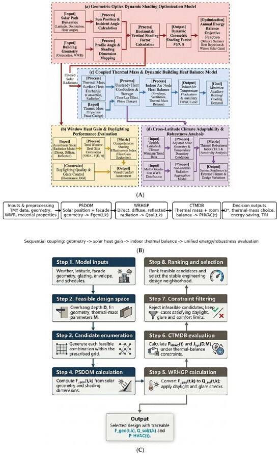
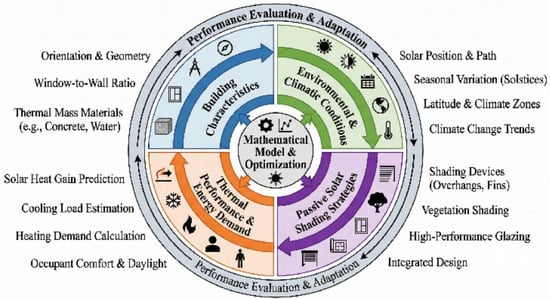
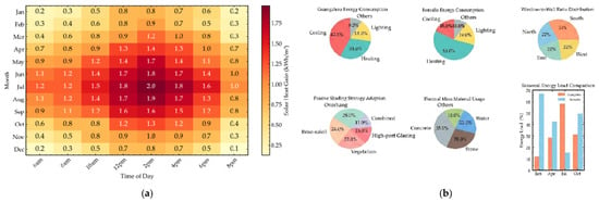
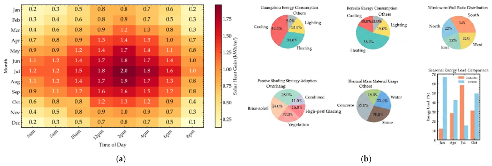
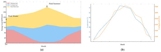
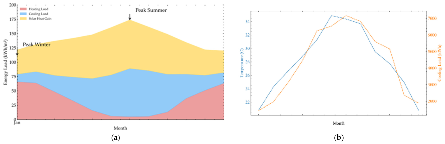
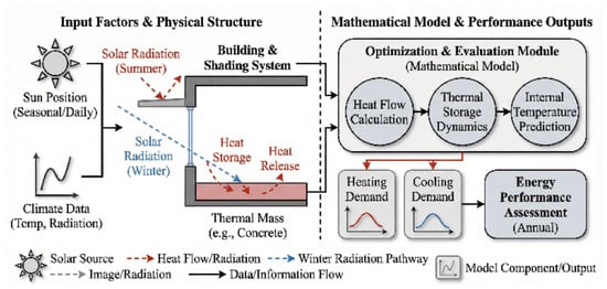
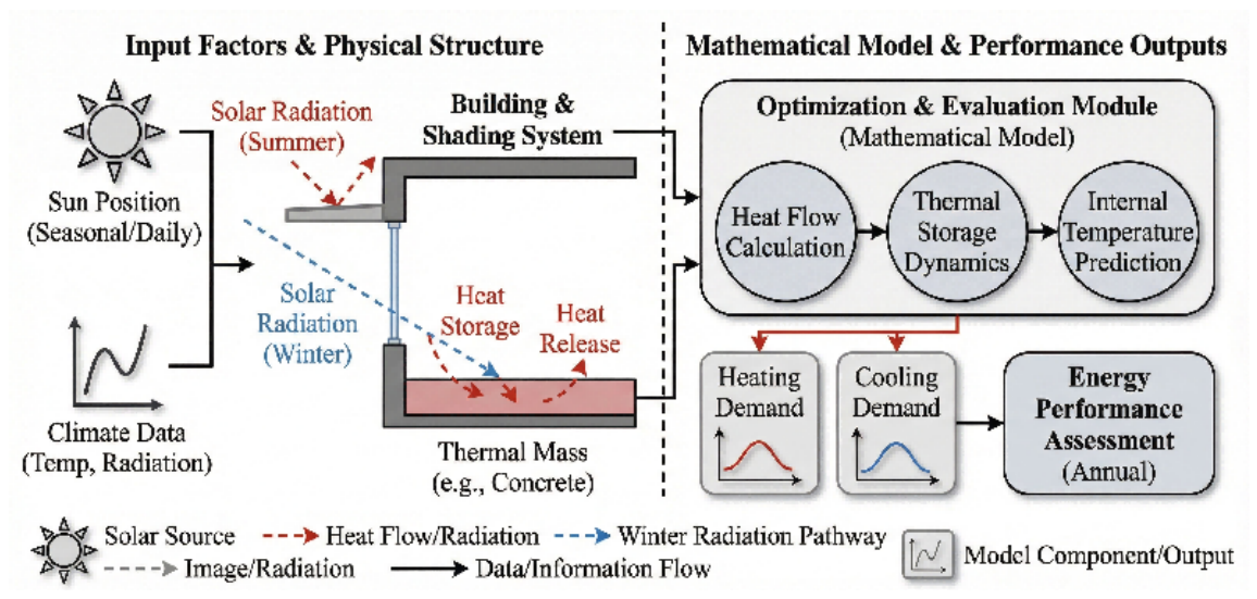
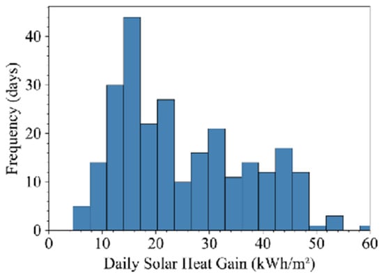
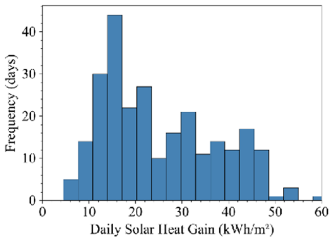
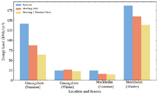
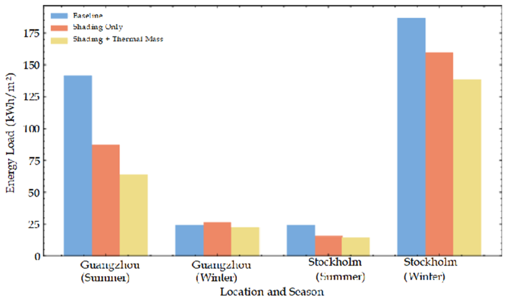
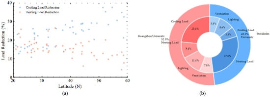
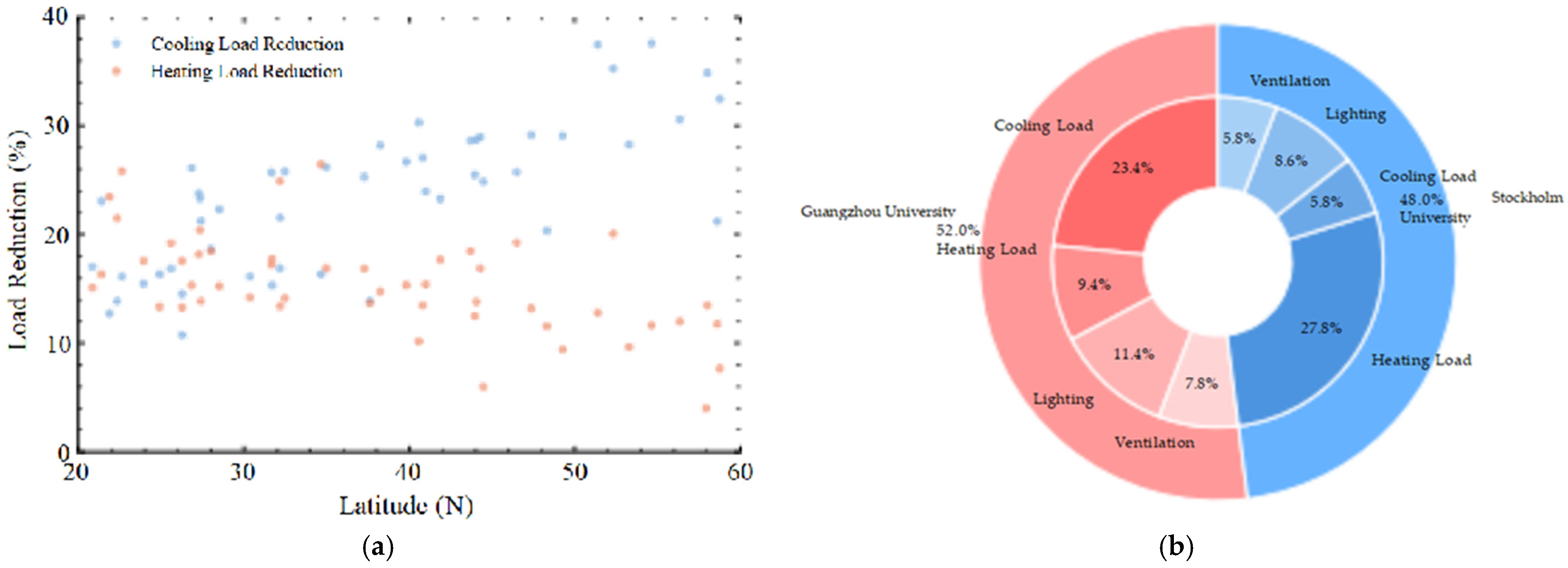
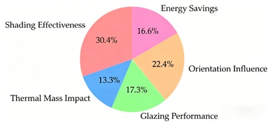
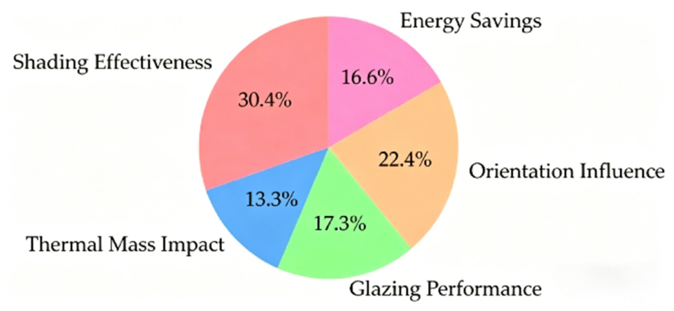
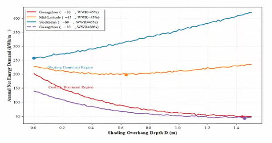
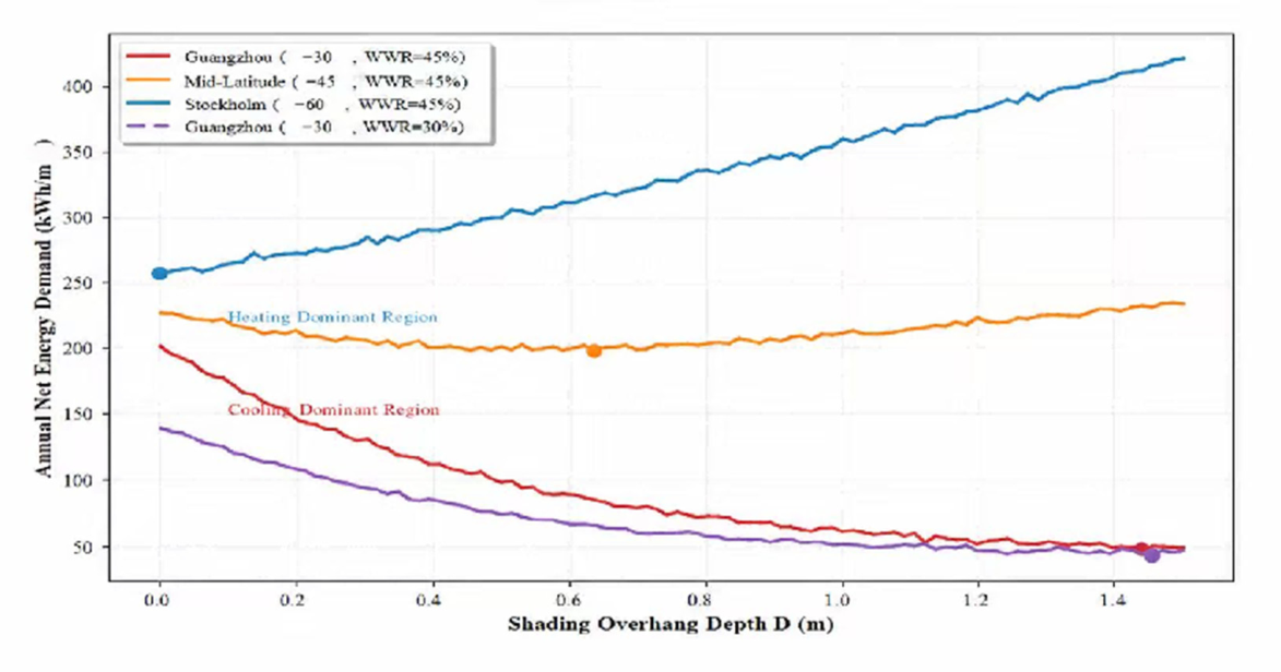

Disclaimer/Publisher’s Note: The statements, opinions and data contained in all publications are solely those of the individual author(s) and contributor(s) and not of MDPI and/or the editor(s). MDPI and/or the editor(s) disclaim responsibility for any injury to people or property resulting from any ideas, methods, instructions or products referred to in the content. |
© 2026 by the authors. Licensee MDPI, Basel, Switzerland. This article is an open access article distributed under the terms and conditions of the Creative Commons Attribution (CC BY) license.