Shear Strength Prediction of Slender Steel Fiber Reinforced Concrete Beams Using a Gradient Boosting Regression Tree Method

Abstract

For the design or assessment of concrete structures that incorporate steel fiber in their elements, the accurate prediction of the shear strength of steel fiber reinforced concrete (SFRC) beams is critical. Unfortunately, traditional empirical methods are based on a small and limited dataset, and their abilities to accurately estimate the shear strength of SFRC beams are arguable. This drawback can be reduced by developing an accurate machine learning based model. The problem with using a high accuracy machine learning (ML) model is its interpretation since it works as a black-box model that is highly sophisticated for humans to comprehend directly. For this reason, Shapley additive explanations (SHAP), one of the methods used to open a black-box machine learning model, is combined with highly accurate machine learning techniques to build an explainable ML model to predict the shear strength of SFRC slender beams. For this, a database of 330 beams with varying design attributes and geometries was developed. The new gradient boosting regression tree (GBRT) machine learning model was compared statistically to experimental data and current shear design models to evaluate its performance. The proposed GBRT model gives predictions that are very similar to the experimentally observed shear strength and has a better and unbiased predictive performance in comparison to other existing developed models. The SHAP approach shows that the beam width and effective depth are the most important factors, followed by the concrete strength and the longitudinal reinforcement ratio. In addition, the outputs are also affected by the steel fiber factor and the shear-span to effective depth ratio. The fiber tensile strength and the aggregate size have the lowest effect, with only about 1% on average to change the predicted value of the shear strength. By building an accurate ML model and by opening its black-box, future researchers can focus on some attributes rather than others.

1. Introduction

Shear failure of reinforced concrete beams is a significant concern due to its brittle and sudden nature [1]. Traditional steel stirrups used as shear reinforcement have been shown to enhance shear capacity efficiently as well as prevent concrete failure. However, incorporating stirrups in narrow, asymmetrical, or congested areas might be challenging. Placing concrete can become a concern when the spacing between stirrups is small, leading to voids in the concrete [2]. Furthermore, traditional stirrups need much labor effort, resulting in more significant building expenses.

In recent years, steel fibers (SF) have acquired significant impetus when utilized in suitable volume fractions due to their potential to replace minimum shear reinforcement [3,4]. Therefore, it has been suggested that implementing SF in the construction industry could provide several advantages. First, SF can enhance the shear resistance by reducing cracks’ width due to the transmission of tensile loads across diagonal cracks, as indicated by Dinh [3]. Concrete shrinkage behavior and post-cracking toughness can also be improved using SF [5,6]. Additionally, the SF inclusion enhances the resistance of the dowel action, which is due to an increase in the tensile strength of the concrete along with the reinforcements in the splitting plane [7].

Various experimental and computational investigations on steel fiber reinforced concrete (SFRC) have been conducted in the literature to examine the shear strength capability [8]. Furthermore, an analysis of the ultimate behavior of SFRC beams was carried out using finite elements and experimental modeling approach utilizing ANSYS software [9]. Additionally, the shear strength of concrete beams with fibers was predicted using a basic physical design model developed by Spinella et al. [10], which considered crack width and shear crack slips. Moreover, utilizing the slenderness ratio, an equation based on fundamental mechanic principles has been proposed to predict the shear strength of SFRC beams [11]. Additionally, SFRC has been studied extensively by conducting several shear experiments on prismatic beams [12].

Several empirical formulas for estimating the shear strength of SFRC beams have been developed in prior research during the last four decades. References [13,14] provide an overview of the most current shear design models and design guidelines for SFRC beams without stirrups. However, the range of validity of such empirical models is limited, which constitute a significant disadvantage. These models are built on the basis of a small number of data specimens, and their accuracy, when applied to additional data cases that fall beyond their range of validity, is arguable. According to a comparison made by references [13,15], it is still challenging to accurately predict the shear capacity of SFRC beams using the various shear resistance models for SFRC. In addition, shear strength predictions from different methodologies differ from one another and still differ from experimentally determined shear strengths. Given these uncertainties, a proper assessment of the reliability of SFRC beams in the event of shear failure is essential. For this, the predictive model must show the highest possible accuracy and the lowest possible variability.

An increase in the use of artificial intelligence (AI) has taken place in recent years due to innovations in computing. Machine learning (ML) models are built using extensive databases. As a result, they can significantly increase generalization capacity and accuracy for measuring the strength of concrete built with various mixing proportions. Therefore, researchers have been inspired by ML and AI to develop new models that can effectively predict the shear capacity of SFRC beams, while overcoming the abovementioned disadvantages. However, despite the emergence of those models, some researchers have focused on some ML methods rather than others for predicting the shear strength of SFRC beams. Support vector machines and artificial neural networks (ANNs), for example, have been widely utilized to predict the mechanical strength of SFRC beams [5,16,17,18,19,20]. Another popular technique utilized for modeling the shear strength of SFRC beams is gene expression programming (GEP) [21,22,23,24,25,26]. However, there is still room for improvement of the prediction of the shear capacity of SFRC beams, even though ANN and GEP algorithms have been widely utilized in various researches concerning the shear capacity prediction of SFRC beams.

In this research, a highly efficient and widely used ML technique, called gradient boosting regression tree (GBRT), is adopted to simulate the process of predicting the shear strength of SFRC beams. GBRT is a powerful ML technique that employs several weak learners and is specifically intended to minimize overfitting issues [27]. Recent research has shown that GBRT shows an excellent prediction performance when compared with other ML algorithms [28,29,30]. Many researches have used GBRT to tackle civil engineering challenges [31,32,33,34].

While some ML-based techniques, such as random forest, neural networks, and support vector machine, can effectively solve regression problems, their operation is difficult to comprehend as these models are often referred to as “black-box” models [35]. As a result, ML-based models should be better described or interpreted to help researchers to better grasp the underlying mechanisms, such as how input parameters impact outputs and increase the persuasiveness of the created models. The Shapley additive explanations (SHAP) framework introduced by Lundberg and Lee [36] can be utilized to understand ML models. In SHAP, features are quantified based on their impact on the predictions. In addition to being able to explain the ML models globally, SHAP can also explain the ML models locally by looking at how the features impact the outputs for a single sample. The research in [37] used GBRT and SHAP for “Understanding the Factors Influencing Pedestrian Walking Speed over Elevated Facilities”. Three ensemble ML models were developed by [38] to predict the creep behavior of concrete, and SHAP was utilized to interpret the predictions of the models. Last but not least, the XGBoost model was developed in reference [39] for load-carrying capacity prediction, and SHAP was used to interpret the ML models.

This study proposes an explainable ML-based technique for predicting the shear strength of SFRC beams. To the best of the authors’ knowledge, the GBRT model is used for the first time to forecast the shear strength of SFRC slender beams. Furthermore, by interpreting the ML model through SHAP, variables impacting the shear strength of the SFRC beams are quantitatively investigated. For this, a database with 330 beam tests, whose shear strength was reported in the literature, was prepared. In addition, the GBRT model’s optimal hyperparameters were identified using a five-fold cross-validation procedure. Additionally, the GBRT model’s performance was compared to other empirical and ML-based equation models presented by other researchers. Finally, the SHAP approach was used to interpret the GBRT model that was built. The effects of several factors on the GBRT model outputs were also explored.

2. Materials and Methods

2.1. Research Methodology

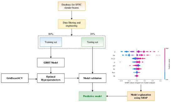
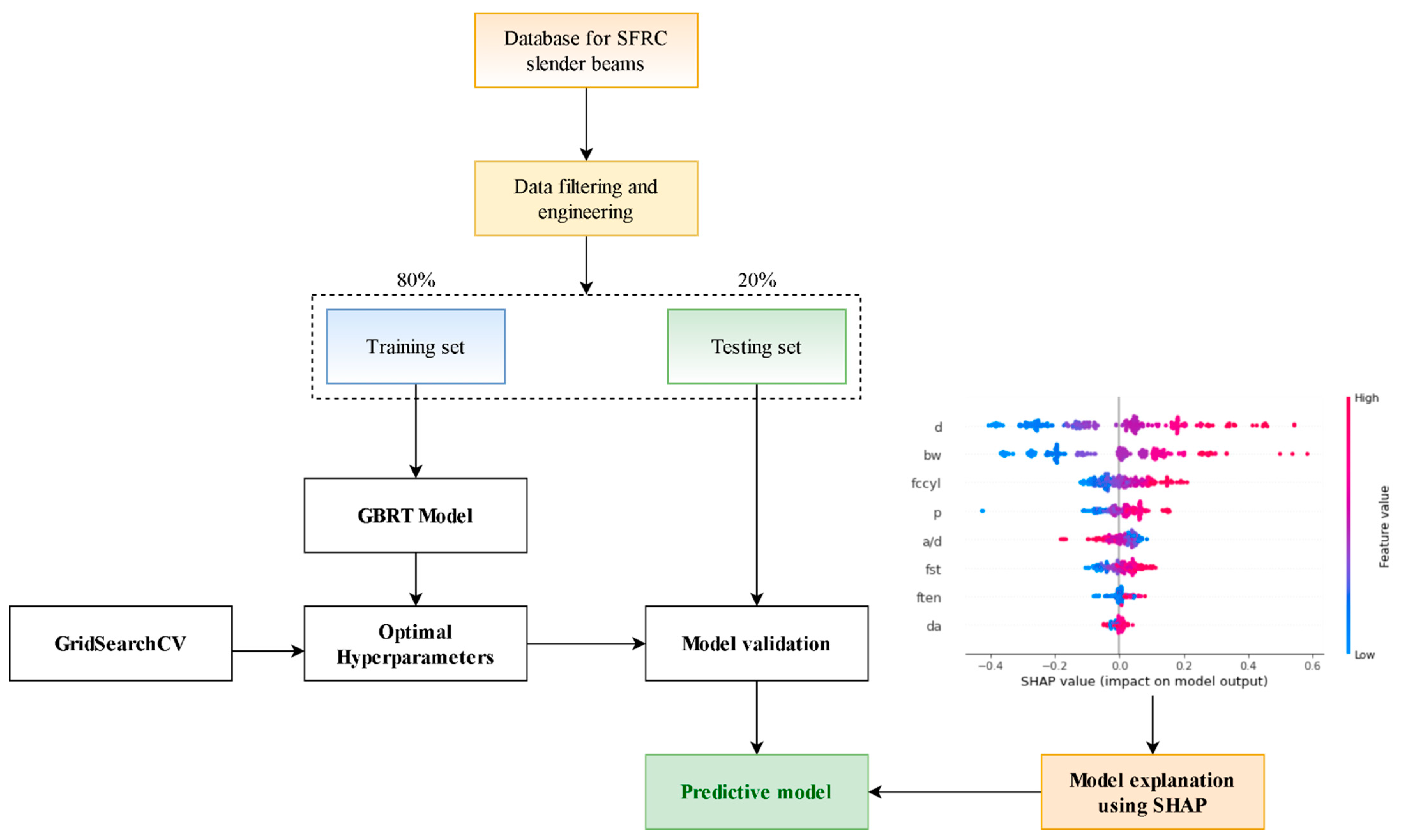
Figure 1 depicts the whole workflow used to develop the suggested approach. The development of a database with SFRC slender beams was the initial stage. After that, some engineering features and filtering methods were applied to the gathered data. The third stage consisted in randomly dividing the data into two sets: one for training and the other for testing. The GBRT model was trained using the training set, and the model was validated using the testing set. The appropriate hyperparameters of the GBRT model were determined by using the five-fold cross-validation procedure during the training stage, this being the fourth stage. The fifth stage includes using the testing set to verify the performance of the model after it has been optimized for the hyperparameters. If the model performance is satisfactory, it can be termed as a final predictive model. During the final process, the SHAP approach is used to understand the model. Quantitatively, the SHAP approach was used to examine how features impact GBRT model predictions on a large dataset (global interpretation) and on a single sample (sample-specific interpretation or local interpretation). As a result, it is possible to analyze the factors influencing the outputs.

Figure 1. Workflow used to develop the explainable ML model.

2.2. Dataset

The shear strength of SFRC beams without shear stirrups has been studied in several experiments. Ref. [13] recently compiled a wide database with 488 experiments on SFRC beams without stirrups. Non-slender beams with a shear-span to effective depth ratio of a/d < 2.5 and beams with shear-flexural mode failure were filtered out of the initial 488 trials, leaving a subset containing 330 experimental tests. The database with 330 experiments was used to build the model and is summarized in Appendix A. The evaluation database contains rectangular and flanged slender beams. The database specimens failed substantially by shear compression and diagonal stress with an a/d ratio higher than 2.5. The experimental database includes shear beams with varying geometry and reinforcement. Based on several studies [10,11,13,14] and to build an efficient ML model, several critical parameters that affect the shear strength of SFRC beams were chosen. Table 1 shows the statistical properties of the evaluation database’s primary parameters. The primary parameter is the shear strength V_u as the output variable, whereas the beam effective depth d, beam width b_w, longitudinal reinforcement ratio ρ, concrete compressive strength f_c, aggregate size d_a, shear span to effective depth ratio a/d, tensile strength of fiber f_t, and steel fiber factor F_sf were considered as predictors. The steel fiber factor depends on the percentage volume V_f, diameter d_f, and fiber length L_f (Equation (1)).

$$F_{sf}=\frac{V_{f }{L}_f}{d_f}$$

(1)

Table 1. Statistical measures of the variables.

Statistics	ft (MPa)	da (mm)	ρ	fc (MPa)	a/d	bw (mm)	d (mm)	Fst	Vu (kN)
Median	1100.0	10.0	0.03	40.7	3.4	150.0	251.0	0.55	108.0
Mean	1269.8	10.5	0.03	48.7	3.4	157.9	282.0	0.61	153.2
Minimum	260.0	0.4	0.004	9.8	2.5	55.0	85.3	0.11	13.0
Maximum	4913.0	22.0	0.06	154.0	6.0	610.0	1118.0	3.82	1481.0
Range	4653.0	216.0	0.05	144.2	3.5	555.0	1032.8	3.71	1468.0
Standard deviation	470.3	5.1	0.01	25.8	0.6	68.7	178.0	0.40	168.9

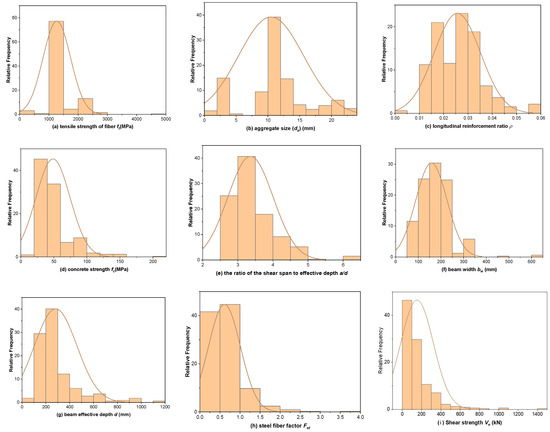
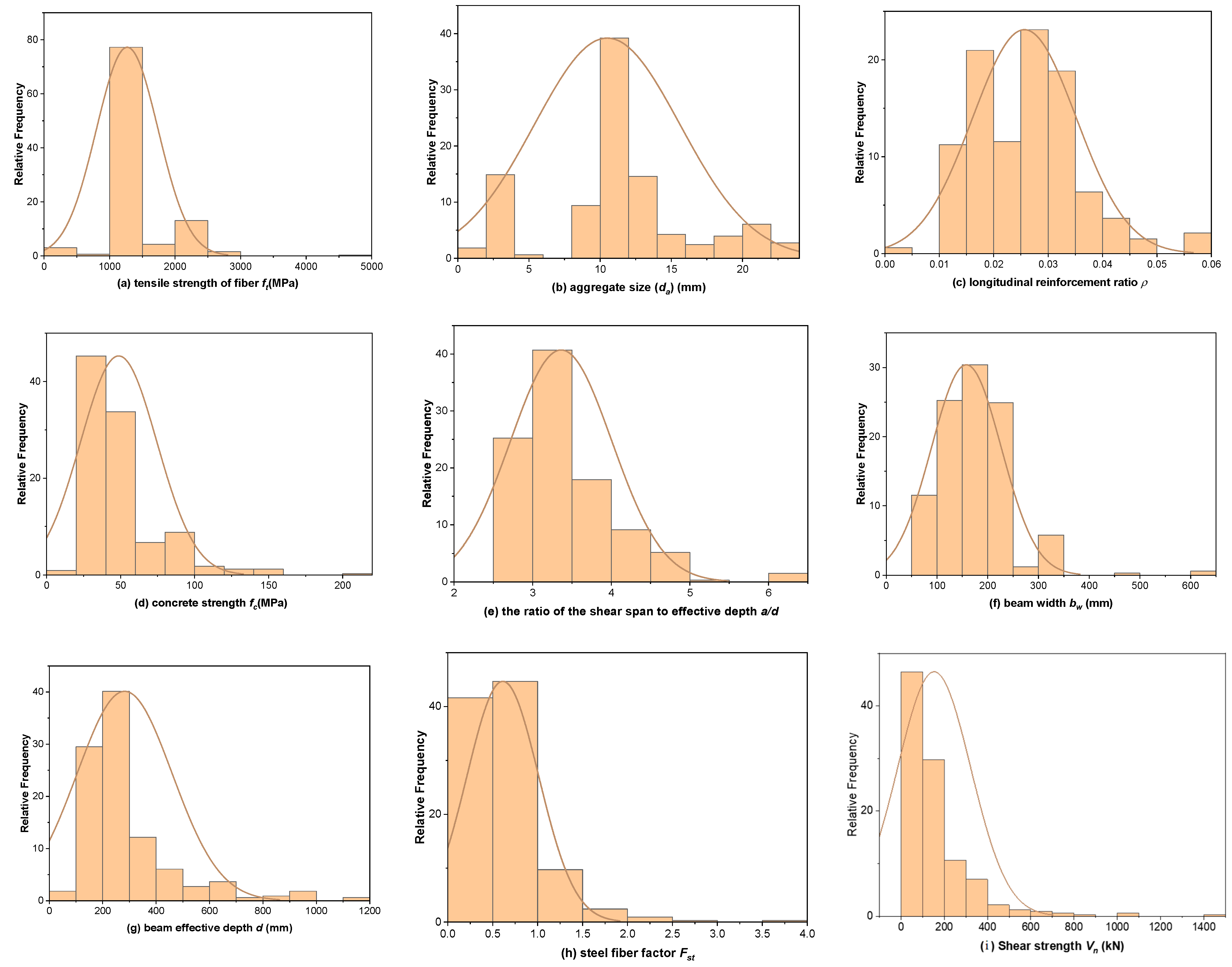
The histograms for the input and output variables from the evaluation database are presented in Figure 2. In general, the database’s range of parameters matches what can be found in real design scenarios, as illustrated in Table 1 and Figure 2. Despite the lack of data for beams with large sizes, the dataset is thought to be representative of most real-world applications and design conditions covered by existing design codes.

Figure 2. Relative frequency distributions for the input and output variables.

2.3. Data-Splitting Procedure

The developed database from the previous section was divided into two parts to implement the ML model: the training dataset and the testing dataset. The GBRT model was developed using the training database, whereas the same predictive model was evaluated using the testing database. As much as possible, a statistically significant association was ensured between inputs of the training and testing datasets while dividing the database into subsets. Most of the developed database (80% of 330 tests) was used for training, while the remaining part was used for model testing (66 tests).

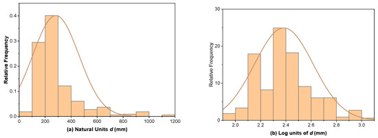
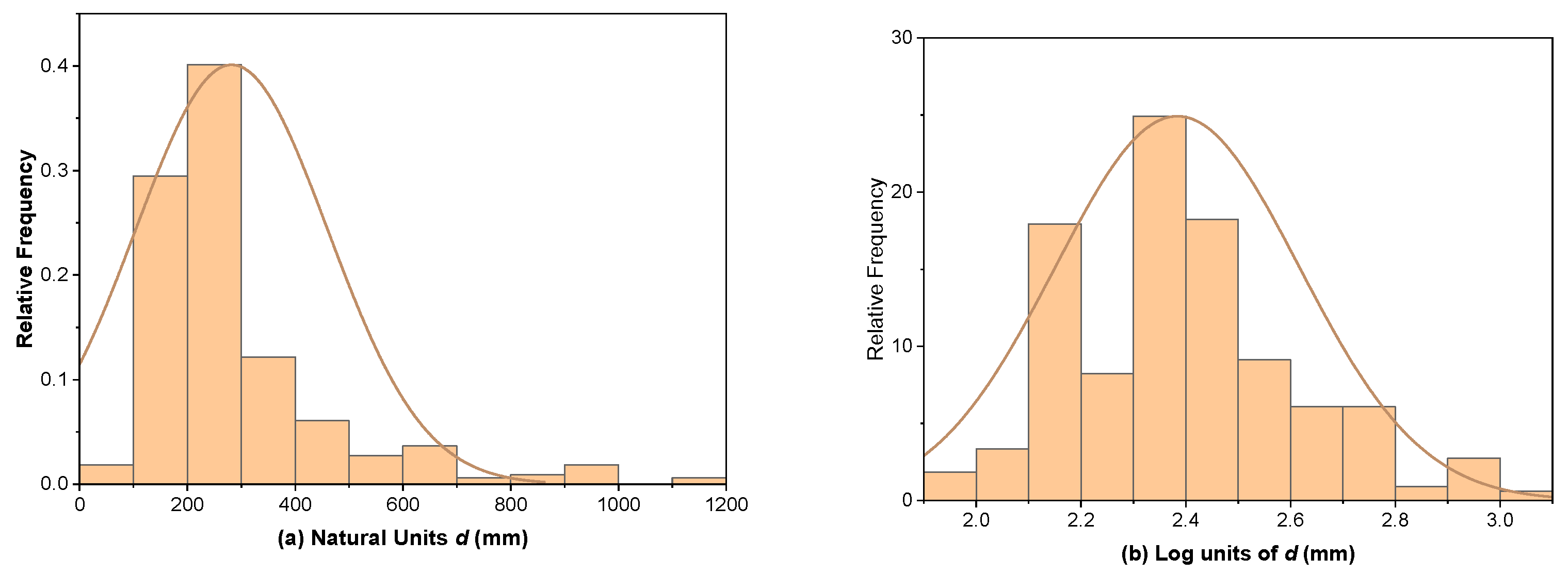
As can noticed from Figure 2, some of the predictors and outcome variables do not obey the normal distribution curve. As a result, these variables need a feature transformation to prevent larger numeric ranges from dominating smaller numeric ranges [40]. In this case, the log transformation was applied to bring right- or left-skewed distributions to approximately normal distributions. Figure 3 shows the distribution of beams’ effective depths (d) before and after log transformation.

Figure 3. Histogram of beam effective depths: (a) before log transformation; (b) after log transformation.

2.4. GBRT Model Development

GBRT uses a statistical boosting method to improve the classic decision tree approach. In this method, instead of creating a single “optimal” model, this strategy aggregates several “weak” models to generate a single “strong” consensus model [41]. When using GBRT, the existing residuals are used to build new decision trees sequentially. Fundamentally, this is a form of a functional gradient descent approach for creating sequential models. Adding a new tree at each stage reduces the loss function, thereby improving the prediction [42].

Training data are assumed to exist in the form of a training set ${\left\{\left(x_i,y_i\right)\right\}}_{i=1}^N$, in which $x_i$ represents the input features and $y_i$ represents the shear capacity. For example, the squared error, the absolute error, the Huber error, etc., are all possible loss functions $L\left(y,F\left(x\right)\right)$ that can be used to measure how much the predicted $F\left(x\right)$ differs from the true shear strength $y$. The GBRT framework assumes that D decision trees will be built, and hence it begins with an initial model $F_0\left(x\right)$. For each iteration d = 1, 2, …, D, compensating the residues is equivalent to optimizing the expansion coefficients ${\rho }_d$ and ${\alpha }_d$ as shown in Equation (2):

$$\left({\rho }_d,{\alpha }_d\right) = {\mathrm{argmin}}_{\rho ,\alpha }{\displaystyle \sum }_{i=1}^{N}L\left[y_i,F_{d-1}+\rho h\left(x_i;\alpha \right)\right]$$

(2)

where $\mathrm{argmin}$ is an operation that finds the argument that gives the minimum value from a target function, and $L\left[y_i,F_{d-1}\right]$ is a pre-selected feasible loss function measuring the amount of how the predicted value $F\left(x\right)$ deviates from the true response y. The weighting coefficients and the base learners are fitted to the training data $x$ in a greedy manner as follows:

$$F_d\left(x\right) = F_{d-1} + {\rho }_{d}h\left(x;{\alpha }_d\right)$$

(3)

Equation (2), on the other hand, is difficult to solve directly. Even so, since the gradient-boosting model is additive, $\rho h\left(x_i;\alpha \right)$ may be seen as an increment along $h\left(x_i;\alpha \right)$. It is possible to find the optimum ${\alpha }_d$ using the least squares method, based on the principle of gradient descent:

$${\alpha }_d={\mathrm{argmin}}_{\alpha ,\beta }{\displaystyle \sum }_{i=1}^N{\left[r_i-\beta h\left(x_i;\alpha \right)\right]}^2$$

(4)

where $\beta$ is a weight factor and $r_i$ is the negative gradient evaluated using the previous model.

$$r_i=-{\left[\frac{\partial L\left(y_i,F\left(x_i\right)\right)}{\partial F\left(x_i\right)}\right]}_{F\left(x\right)=F_{d-1}\left(x\right)},i=1,\cdots ,N$$

(5)

One-dimensional optimization can be used to further improve the gradient-descent step size or weight of the obtained decision tree:

$${\rho }_d={\mathrm{argmin}}_{\rho }{\displaystyle \sum {}_{i=1}^N}L{[r_i,F_{d-1}+\rho h(x_i;{\alpha }_d)]}^2$$

(6)

Finally, according to Equation (3), the prior model will be added to the newly evaluated residue model. Algorithm 1 represents the pseudocode for the generic gradient boosting.

Algorithm 1. The gradient boosting algorithm.

Input the iteration number D, loss function $L\left(y,F\left(x\right)\right)$ training set ${\left\{\left(x_i,y_i\right)\right\}}_{i=1}^N$ Initialize: F0 = ${\mathrm{argmin}}_{{\rho }_0}{\displaystyle \sum {}_{i=1}^N}L(y_i,{\rho }_0)$ For d = 1 to D do: $r_i = -{\left[\frac{\partial L\left(y_i,F\left(x_i\right)\right)}{\partial F\left(x_i\right)}\right]}_{F\left(x\right)=F_{d-1}\left(x\right)},i = 1,\cdots ,N.$ ${\alpha }_d ={\mathrm{argmin}}_{\alpha ,\beta }{\displaystyle {\displaystyle \sum }_{i=1}^N}{\left[r_i-\beta h\left(x_i;\alpha \right)\right]}^2$ ${\rho }_d={\mathrm{argmin}}_{\rho }{\displaystyle \sum {}_{i=1}^N}L{[r_i,F_{d-1}+\rho h(x_i;{\alpha }_d)]}^2.$ $F_d\left(x\right) = F_{d-1}+{\rho }_{d}h\left(x;{\alpha }_d\right)$ end for Output: the final regression function Fd(x)

Gradient boosting allows for a wide variety of smooth loss functions, including AdaBoost, LogitBoost, and L2Boosting [43]. Because of its simplicity and coherence in solving regression problems, the squared loss function is employed in this study:

$$L(y,F_D(x))={\displaystyle \sum {}_{i=1}^N}{(y_i-F_D(x_i))}^2.$$

(7)

Regularization techniques are typically used during the training stage to reduce overfitting and to boost the model’s generalization capacity. In the following equation, Gradient boosting uses a new variable called ${\nu }_d$ to regulate the model’s update rate, which is known as shrinkage or learning rate:

$$F_d\left(x\right)=F_{d-1}\left(x\right)+{\nu }_d\cdot {\rho }_{d}h\left(x;{\alpha }_d\right),0<{\nu }_d<1$$

(8)

The model is updated more slowly when ${\nu }_d$ is smaller. According to [44], utilizing small learning rates leads to better model generalization without shrinkage; however, this comes at the cost of greater computing time because more decision trees are required. In addition, numerous additional parameters that are strongly related to the final tree’s structure and model complexity, such as depths (maximum number of splits) and the number of trees D, must be fine-tuned to maximize the performance of the model.

2.5. Cross-Validation

The division of the complete dataset into three subsets—training, validation, and testing—is a standard approach for evaluating the performance of ML models. While the training set is used to complete the learning process, the validation set tracks the performance of the model. As a final step, the model’s extrapolation skills are tested by running it through a set of samples that it has never seen before (testing set) [40]. However, dividing data into three subsets reduces the size of the dataset, which might result in an inadequately trained model. As a result, cross-validation is a typical strategy for avoiding over-reduction of the training set, particularly for small datasets [40]. Cross-validation is performed in various ways, the most common of which is omitting random data to verify the model. K-fold cross-validation was used in this research. Cross-validation with K-fold is a resampling technique that divides data into k subsets, one for validation and the other k-1 for training.

2.6. Hyperparameter Tuning

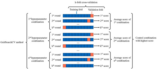
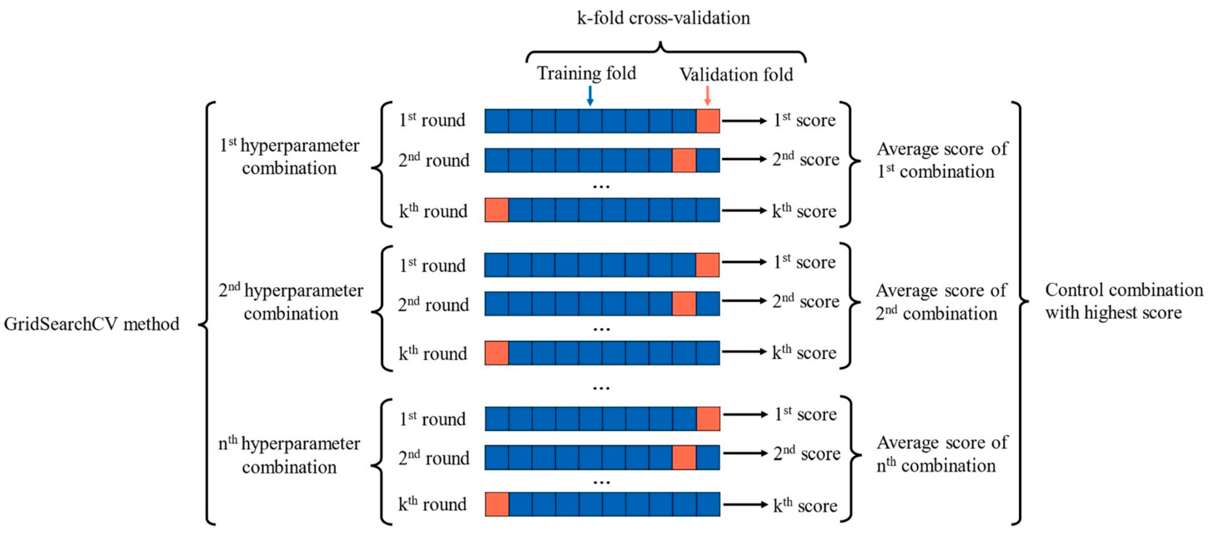
The tuning of hyperparameters is an essential step in developing reliable ML models. Tuning an ML model reduces overfitting and increases the model adaptability to new data [45]. Choosing the best hyperparameters is also a key component in improving the accuracy of the model [46]. Many ways to automate hyperparameter selection have been developed to prevent manual tuning, including grid search and random search hyperparameter optimization [47]. The domain of the possible values evaluated in the search effort distinguishes these techniques from each other. Random search methods choose distinct hyperparameter values randomly for a given number of iterations, while grid search investigates all potential values in a pre-defined domain for the hyperparameters [47]. The Scikit-learn package in Python [48] was used to explore possible values of hyperparameters using a grid search technique with five-fold cross-validation (GridSearchCV). Figure 4 depicts the five-fold cross-validation used in this work for training and for the hyperparameter selection of the model.

Figure 4. Hyperparameter tuning using five-fold cross validation (GridSearchCV).

2.7. Performance Metrics

2.7.1. Model Performance Metrics

Various statistical measures, such as R², mean absolute error (MAE), root mean squared error and (RMSE), were used to evaluate the performance of the built ML-based models. For example, the best model has an R² value close to 1, while RMSE and MAE values are close to zero. In order to obtain the MAE value, the absolute difference between actual and predicted values must be averaged. The equation for MAE is the following one:

$$MAE = \left(\frac{{{\displaystyle \sum }}_{i=1}^n\left|y_i^{obs}-y_i^{pre}\right|}{n}\right)$$

(9)

When the R² value is 1, the predicted and true/actual values are perfectly aligned. R² has the following mathematical representation:

$$R^2=\frac{{\displaystyle \sum _{i=1}^n{(y_i^{obs}-y^{-obs})}^2}-{\displaystyle \sum _{i=1}^n{(y_i^{obs}-y_i^{pre})}^2}}{{\displaystyle \sum _{i=1}^n{(y_i^{obs}-y^{-obs})}^2}}\in [0,1].$$

(10)

where y_i^obs and y_i^pre are the actual output and predicted values, respectively, and y^−obs is the average of all observed data.

The difference between the predicted and actual values is the error and the RMSE is calculated as the square root of the average squared errors. The RMSE is computed as follows:

$$RMSE=\sqrt{\frac{1}{n}{\displaystyle \sum }_{i=1}^n{\left(y_i^{obs}-y_i^{pre}\right)}^2}$$

(11)

2.7.2. Model Uncertainty Metrics

The model uncertainty, or standard deviation (scatter) of the model error, and the mean (bias) are used to evaluate the built models. Due to the lack of knowledge of the problem, conservative assumptions, and mathematical simplifications, the model uncertainty is defined as a model inability to effectively reflect and express a physical phenomenon (in this case, the shear strength). The model uncertainty is described as a random variable with a standard deviation, mean value, and probability distribution in the structural reliability framework. Shear reliability analysis has been proven to be significantly impacted by it. In this work, the predictive model uncertainty related to beam x is equal to the ratio between the experimental and the predicted shear strength, as stated in Equations (12) and (13).

$$M_x=\frac{R_{\exp ,}}{R_{pred,x}\left(X\right)}$$

(12)

$$M\left({\mu }_M,{\sigma }_M\right)$$

(13)

For a single beam test x, M_x is the model uncertainty. The predictors for the GBRT model (a/d, d, b_w, ρ, f_c, f_t, d_a, and F_sf) are represented by X. The mean and standard deviation of the model uncertainty are represented by ${\sigma }_M$ and ${\mu }_M$, respectively.

It is better to choose a model with a mean ${\mu }_M$ close to 1 and a standard deviation ${\sigma }_M$ close to 0 for the model uncertainty. ${\mu }_M$ > 1 indicates that the model underestimates the shear capacity of the beam specimen and, consequently, underestimates its failure load. However, if ${\mu }_M<1$, it suggests that the model overestimates the shear resistance.

2.8. Shapley Additive Explanations (SHAP) Framework

Lately, Explainable black-box ML models have attracted more study interest because they allow users to trust the created ML models by helping them to comprehend the ML models’ involved mechanism. SHAP is a method for explaining “black-box” ML models. Lundberg and Lee [36] were the first to suggest SHAP, which is based on the notion of Shapley game theory. The SHAP seeks to assess the contribution of each input variable or feature to the observation, and it can determine whether the contribution of each feature is positive or negative. To help with the global and local explanation of ML models, SHAP can calculate the contribution from each feature for every observation. SHAP creates a model of explanation that can be written as:

$$g(z^{\prime })={\varphi }_0+{\displaystyle \sum _{j=1}^K{\varphi }_j{z}_j^{\prime }}$$

(14)

where $z^{\prime }\in {\{0,1\}}^K$ and K represent the number of input features; ${\varphi }_j\in ℝ$ is the SHAP value for the j–th feature; ${\varphi }_0$ is the constant if all inputs are missing.

The SHAP value for the j–th feature can be calculated as:

$${\varphi }_j={\displaystyle {\sum }_{S\subseteq F\backslash \left\{i\right\}}\frac{\left|S\right|!\left(\left|F\right|-\left|S\right|-1\right)!}{\left|F\right|!}}\left[f_{S\cup \left\{i\right\}}\left(x_{S\cup \left\{i\right\}}-f_S\left(x_S\right)\right)\right]$$

(15)

where F is the set of all features and x_S is the value of the input.

2.9. Programming Languages and Softwares

In this research, the Python programming language combined with the Scikit-learn library was used to build the system for the estimation of the shear capacity and the interpretation of the GBRT model. Python is a high-level, easy-to-learn, open-source, extensible, and object-oriented programming language (OOP). Python is also an interpreted and versatile language widely used in many fields, such as for building independent programs using graphical interfaces and web applications. In addition, it can be used as a scripting language to control the performance of many programs. It is often recommended for beginners in programming to learn this language because it is among the fastest programming languages to learn [49].

On the other hand, Scikit-learn [48] is an ML library in Python. It contains many algorithms and methods used in the field of ML, such as classification, clustering, and regression, in addition to being used in the stages of data processing and model evaluation. It was built based on the libraries of Scipy, Numpy, Matplotlib, and many others. This study implemented the data preprocessing, filtering techniques, and GBRT modeling using the Python programming language and the Scikit-learn library. At the same time, the plots and figures were created using OriginLab software.

3. Model Results

3.1. K-Fold Cross-Validation

Before running the model, there is the need to fine-tune several of GBRT’s hyperparameters. The hyperparameters of the GBRT model were optimized using a grid search process and a five-fold cross-validation. The most critical hyperparameters for the GBRT model are the n estimators and the learning rate, representing the number of the model’s weak learners and the weights assigned to each estimator, respectively. Additionally, the GBRT model prediction performance can be considerably affected by its max depth parameter, which indicates the complexity of each tree, and its subsample parameter, which represents the fraction of samples to be used for fitting the individual base learners [50]. The tuned values for each of the four hyperparameters are shown in Table 2. The coefficient of determination (R²) was closely examined as a statistical error to obtain hyperparameters with the maximum accuracy while minimizing over-fitting. To execute GBRT modeling and tuning, the Scikit-learn program [48] was used.

Table 2. Hyperparameters for the GBRT model.

Hyperparameter	n Estimators	Learning Rate	Max Depth	Subsample
Values	1500	0.01	8	0.2

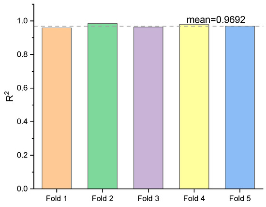
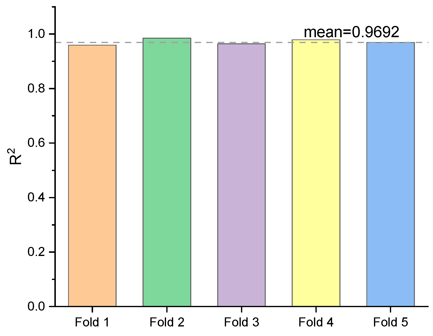
A total of 264 data records was used to train the GBRT model, and 66 samples were used to test it. The five-fold cross validation results are shown in Figure 5. Again, there is no noticeable fluctuation in the results of the five folds, and the overall accuracy remains excellent. For example, Fold 1 has a minimum R² value of 0.9580, and Fold 2 has a maximum R² value of 0.9852. Table 3 provides the full statistical breakdown of the folds’ results. The coefficient of variation (COV) is only 1.1246% based on the average R² of 0.9692 and the standard deviation (SD) of 0.0109.

Figure 5. Results for five-fold cross validation.

Table 3. Cross-validation measurement results.

Statistics	Folds
	1	2	3	4	5	SD	Average	COV%
R2	0.9594	0.9853	0.9644	0.9790	0.9692	0.0109	0.9692	1.1246

3.2. GBRT Performance on Testing Set

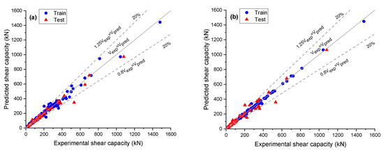
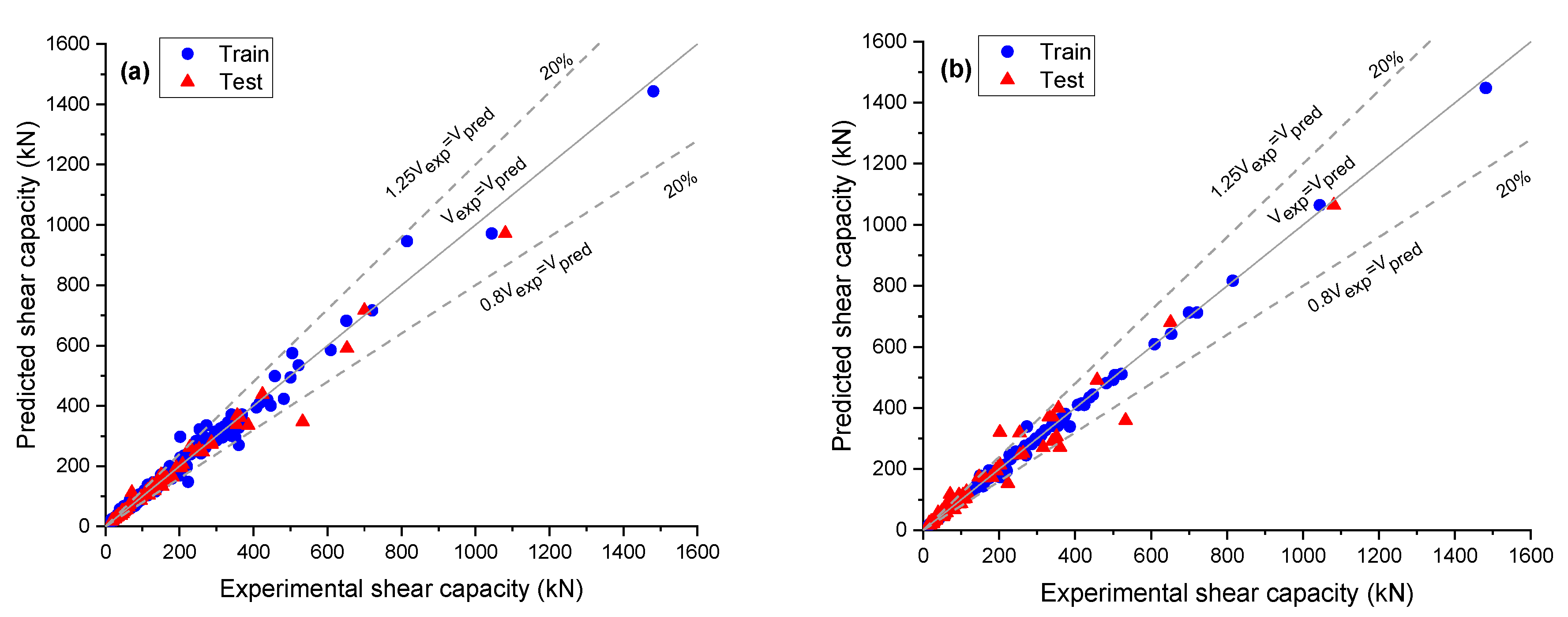
The prediction performance of the proposed method can be tested after the hyperparameters have been identified. The prediction findings are shown in Figure 6, with the X and Y axes representing the experimental and predicted shear strengths, respectively. The training and testing outcomes are represented by the blue dot and red triangle, respectively. In most cases, the difference between the predicted and actual shear strength is within a margin of error of 20% or less. There were three further iterations of the experiment, each using a different mix of training and testing datasets. The predictions for all four experiments are reported in Table 4. The testing RMSE and MAE were always less than 30 and 17, respectively. The mean absolute percentage error, or MAPE, was less than 14%. That is to say, for every sample and instance, the deviation between the predicted and actual shear strength was less than 17 kN (equivalently 14%). These results show that the GBRT approach can be considered an effective tool for estimating the shear capacity of SFRC beams.

Figure 6. Prediction results: (a) case 1; (b) case 3.

Table 4. Testing results of four repeated experiments.

Experiment	RMSE (kN)	MAE	MAPE	R2
Case 1	29.561	16.444	0.1369	0.943
Case 2	19.276	9.410	0.065	0.977
Case 3	15.44	8.313	0.057	0.990
Case 4	25.49	12.56	0.067	0.978

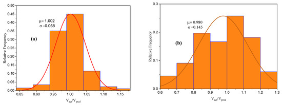
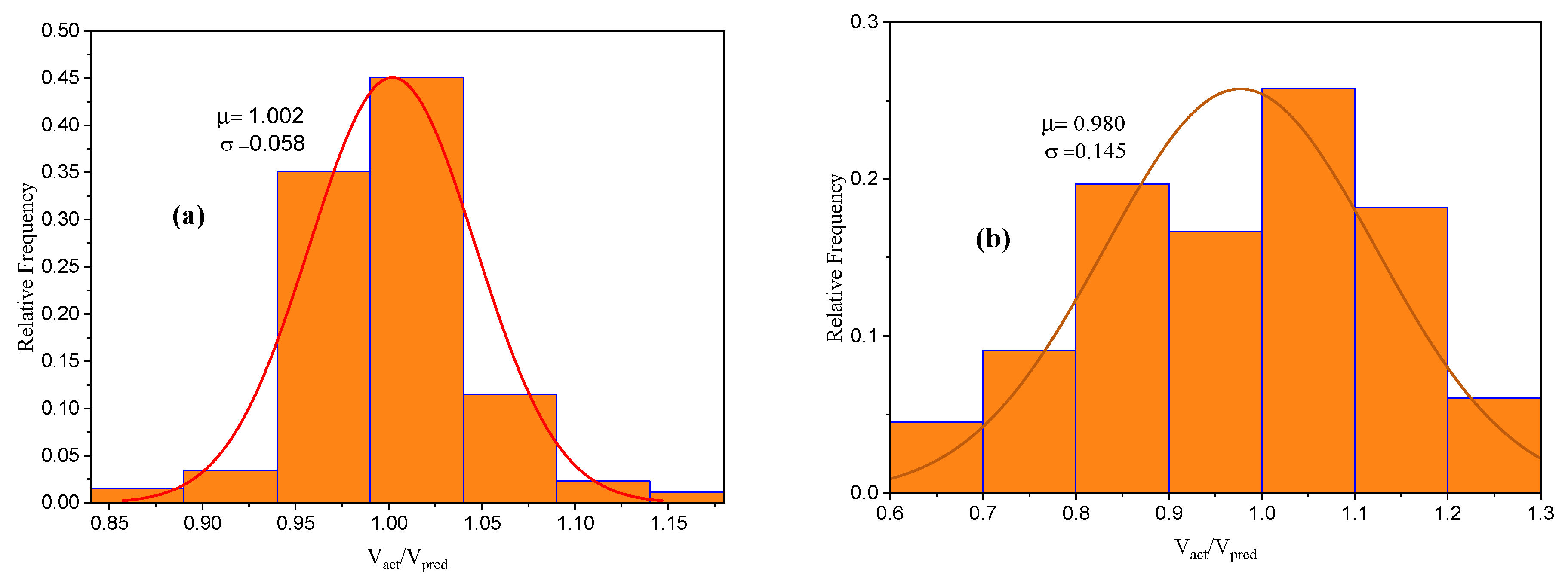
Figure 7 presents the histogram of the predicted shear strength (V_pred) from the GBRT model compared to the actual shear strength (V_act) (case 1). Again, most of the shear strengths predicted by GBRT are within a margin of 20% or less of error. The standard deviation $\left({\sigma }_M\right)$ and mean value (${\mu }_M$) of the ratio V_act/V_pred are taken into consideration when evaluating the accuracy of the GBRT model. The standard deviations (${\sigma }_M$) for the training and testing data were 0.058 and 0.145, respectively, whereas the mean values (${\mu }_M$) were 1.002 and 0.980, respectively. A normally distributed relationship between the GBRT-predicted values and the experimental data shows that the error is dispersed randomly.

Figure 7. Histogram for V_act/V_pred (case 1): (a) training set; (b) testing set.

3.3. The Reliability of the GBRT Model Prediction

For a total of 330 SFRC beams, the statistical evaluation of the various models [1,21,26,51,52,53] used to estimate the shear strength, and also for the model developed in the present study, can be found in Table 5. The formulas from the models used for the comparative analysis can be found in Table 6. Ashour et al. [52] proposed two sets of equations based on a regression model for observed data gathered from 18 high-strength SFRC beam specimens. An essential parameter, the fiber factor (F), which accounts for the influence of steel fiber size and shape, was incorporated into the first equation, taken from the ACI Building Code’s shear equation. In addition, to account for the role of reinforcement and concrete in the shear capacity, the authors incorporated the shear span to effective depth (a/d) ratio in their equation. The second equation of Ashour et al. [52] is based on a modified version of Zsutty’s equation [54], which includes the fiber factor. Deep beams ($\frac{a}{d}<2.5$) and slender beams ($\frac{a}{d}\ge 2.5$) have unique formulas in the two sets of the second equation. A modified version of the ACI Building Code equation was also established for the shear capacity by Khuntia et al. [1]. In their equation, the effect of fiber is incorporated. Khuntia et al. [1] used the post-cracking tensile properties of fiber reinforced concrete to build the equation. The experimental data of 68 SFRC beam specimens were used to validate the equation. An equation presented by Sharma [51] omits some of the essential parameters, such as the ratio l_f/d_f and F, which substantially impact the shear capacity of SFRC. The referred author used 41 experiments to validate his equation. Rather than incorporating the actual reinforcement ratio, the equation from Greenough and Nehdi [21] simplifies a formula derived from genetic programming by using a percentage for ρ. Additionally, 208 SFRC beam test results from earlier research were analyzed using multi-expression programming to obtain the formula presented by Sarveghadi et al. [26]. The authors have produced two sets of equations: one set contains expressions specific to high-strength concrete, and the other set is a composite equation for both types of concrete (normal- and high-strength). An equation for predicting the shear strength of SFRC beams based on 293 previous experiments was recently published by Sabetifar and Nematzadeh [53]. The previous two studies [26,53] built their models based on genetic programming (GP). GP is a machine learning-based approach for developing nonlinear regression. The Darwinian ideas of natural selection and genetic spreading of features chosen by biologically growing organisms are the foundations of GP. Even though both researches [26,53] were published recently, the datasets utilized to train and test the models were quite constrained, resulting in models with only limited application. The equations for the shear capacity of SFRC beams proposed in the previous referred studies are given in Table 6.

Table 5. Statistical measures of the proposed equations.

Model	${\mathit{\mu }}_{\mathit{M}}$	STD	COV	Min	Max
Sarveghadi et al. [26]	$0.991$	$0.26$	$27\%$	$0.22$	$1.92$
Greenough and Nehdi [21]	$1.20$	$0.37$	$30\%$	$0.31$	$3.11$
Khuntia et al. [1]	$1.48$	$0.45$	$31\%$	$0.18$	$4.03$
Sharma [51]	$1.11$	$0.33$	$30\%$	$0.18$	$2.28$
Sabetifar and Nematzadeh [53]	$0.968$	$0.22$	$22\%$	$0.33$	$1.83$
Ashour et al. [52]	$1.15$	$0.40$	$35\%$	$0.24$	$3.14$
Ashour et al. [52]	$1.35$	$0.35$	$26\%$	$0.47$	$3.22$
Proposed GBRT	0.996	0.08	12%	0.64	1.26

Table 6. Previous equations for the shear capacity of SFRC beams.

Reference	Author	Equation
[26]	Sarveghadi et al.	$\begin{array}{c}{V}_u=\left[\rho +\frac{\rho }{v_b}+\frac{1}{\frac{a}{d}}\left(\frac{\rho f_t^{\prime }\left(\rho +2\right)\left(f_t^{\prime }\frac{a}{d}-\frac{3}{v_b}\right)}{\frac{\frac{a}{d}}{ }}+f_t^{\prime }\right)+v_b\right]b_{w}d\\ f_t^{\prime }=0.79\sqrt{f_c^{\prime }}\\ v_b=0.41\tau F\mathrm{with}\tau =4.15\mathrm{MPa}\end{array}$
[21]	Greenough and Nehdi	$V_u=\left[0.35\left(1+\sqrt{\frac{400}{d}}\right){\left(f_c^{\prime }\right)}^{0.18}{\left(\left(1+F\right)\rho \frac{d}{a}\right)}^{0.4}+0.9{\eta }_o\tau F\right]b_{w}d$
[1]	Khuntia et al.	$V_u=\left[\left(0.167+0.25F\right)\sqrt{f_c{ }^{\prime }}\right]b_{w}d$
[51]	Sharma	$V_u=\left(\frac{2}{3}\times 0.8\sqrt{f_c^{\prime }}{\left(\frac{d}{a}\right)}^{0.25}\right)b_{w}d$
[52]	Ashour et al.	$\begin{array}{c}{V}_u=\left[\left(0.7\sqrt{f_c{ }^{\prime }}+7F\right)\frac{d}{a}+17.2\rho \frac{d}{a}\right]b_{w}d\\ V_u=\left[\left(2.11\sqrt[3]{f_c{ }^{\prime }}+7F\right){\left(\rho \frac{d}{a}\right)}^{0.333}\right]b_{w}d\mathrm{for}\frac{a}{d}\ge 2.5\\ V_u=\left[\left(\left(2.11\sqrt[3]{f_c{ }^{\prime }}+7F\right){\left(\rho \frac{d}{a}\right)}^{0.333}\right)\frac{2.5}{\frac{\pi }{d}}+v_b\left(2.5-\frac{a}{d}\right)\right]b_{w}d\mathrm{for}\frac{a}{d}<2.5\end{array}$
[53]	Sabetifar and Nematzadeh	$V_u=\left[F+2\rho +\sqrt{\frac{\rho f_c^{\prime }{(F+3.58)}^2}{\left(a/d\right)}}-{\rho }^2\left(f_c^{\prime }+8.52\right)+F\left(F-0.73\right)\left({\rho }^{\rho }-\sqrt{a/d}\right)\right]b_{w}d$

where: $f_c^{\prime }$ and $f_t^{\prime }$ are the compressive and tensile strengths of concrete, respectively; $F$ is the fiber factor; ${\eta }_o$ is the fiber orientation factor, $\tau$ is the average fiber–matrix interfacial bond stress.

The mean value for the ratio of the experimental values to the model predicted values (${\mu }_M$) and their variability (CV) was used to evaluate the performance of the model. The prediction is more accurate when ${\mu }_M$ is near to 1 and when the CV is low. As can be observed in Table 5, five of the ${\mu }_M$ values are higher than 1.00, implying that the models from [1,21,51,52] underestimate the shear capacity of SFRC beams, while the models from [26,53] slightly overestimate the shear resistance. The explanation for this observation might be linked to the fact that the previously referred equations were produced based on a limited set of data with low variation between specimens’ properties. Furthermore, the equations proposed in the referred literature omit some critical factors that contribute to the shear strength of SFRC.

With ${\mu }_M$ = 0.996, STD = 0.08, and COV = 12%, it can be stated that the proposed model in this research beat all previous models. As a result, the model has a reduced error rate and a higher degree of linearity between the anticipated and actual values. Furthermore, the GBRT model has the lowest coefficient of variation (COV) when compared to the other models, indicating that its projected values have the slightest variance around the mean.

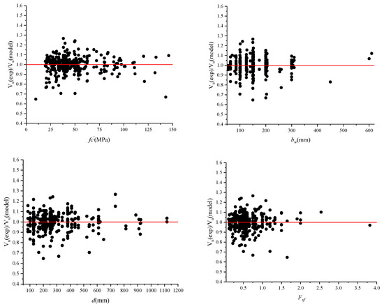
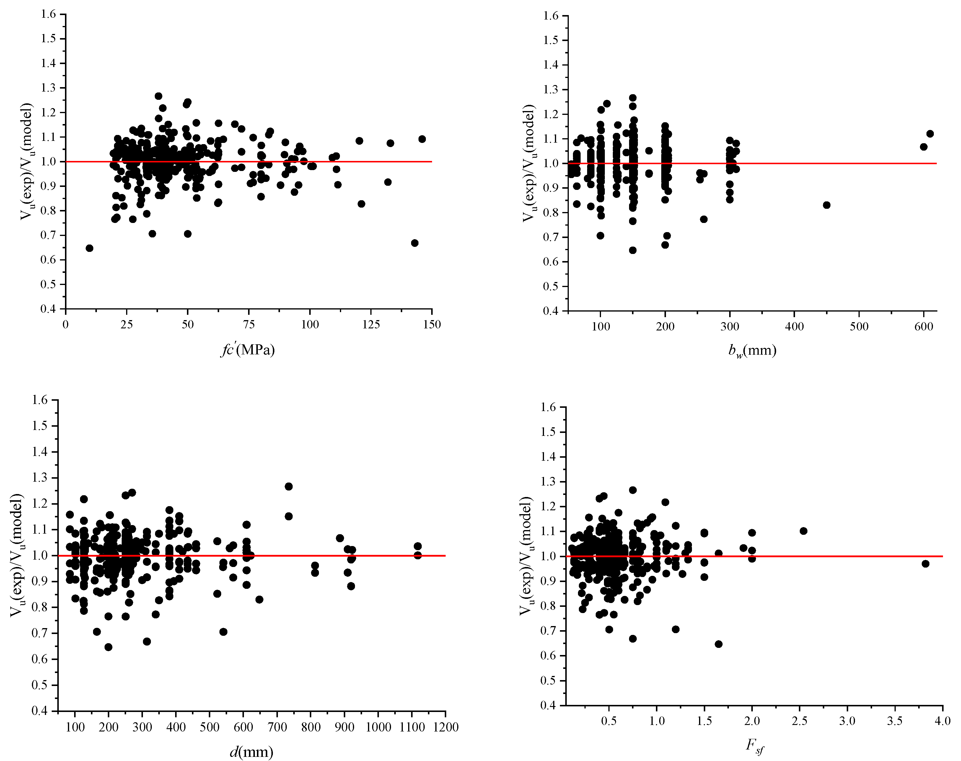
The experimental to prediction ratios for each input variable are presented in Figure 8, in order to check if a bias exists between the prediction of the GBRT model and one or more input variables. From Figure 8, it seems that a significant trend or preference toward these variables does not exist. The accuracy of the GBRT prediction for the shear strength seems robust. This indicates that the proposed model can be employed with high confidence within the ranges of independent variables used to construct the model.

Figure 8. The relationship between the shear input variables and the ratio of experimental to model shear strength.

3.4. Interpretation of the GBRT Model

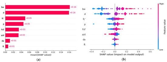
The SHAP approach was used to understand the developed GBRT model and how its inputs impact its outputs. The summary of the SHAP values and the feature importance factor for all of the input features can be seen in Figure 9. Each dot on the graphs represents a dataset instance and its corresponding feature SHAP value. The x-axis indicates each feature’s effectiveness on the dependent variable, while the y-axis shows the model’s ranking of features by significance. A red dot denotes a high feature value, corresponding to a higher SHAP value. The significance of each feature is determined as the mean absolute SHAP values for the whole dataset, as shown in Figure 9a.

Figure 9. The relative importance of each feature and SHAP summary plot: (a) relative importance; (b) SHAP summary plot.

Figure 9a shows that both the beam width (b_w) and the effective depth (d) are the most important factors, followed by the concrete strength (fc) and the longitudinal reinforcement ratio (ρ). In addition, the outputs are also affected by the steel fiber factor (F_sf) and the shear-span to effective depth ratio (a/d). Finally, the fiber tensile strength (f_t) and the aggregate size (d_a) have the lowest effect. According to the results in Figure 9a, b_w and d have the ability to alter the estimated value of shear strength by an average of 16%, while f_t and d_a have the lowest ability with only about 1%. As can be seen in Figure 9b, most of the features mentioned above positively influence the model outcome, which indicates that when one of those features increases, the shear capacity of the SFRC slender beam increases. The only exception among those features is a/d. This observation can be explained due to the influence of the arch action, which depicts the compressive force created along with the beam supports and the loading points. Loads are borne in part by the arch action in the area of small shear spans. The applied shear is resisted by the arch action, which leads to a decreased shear for higher a/d [55]. The conclusions presented in this section can assist constructers and designers in determining the importance of each feature in SFRC slender beams for the output shear strength, and whether it is positive or negative.

4. Conclusions

An investigation on the use of an explainable ML method for the prediction of the shear strength of SFRC slender beams was conducted in this study. Using SHAP to interpret the ML model, the factors impacting the shear strength were examined. A database with 330 SFRC slender beam tests was created and randomly divided into testing and training sets. Using a five-fold cross-validation procedure paired with a grid search strategy, optimal hyperparameters of the GBRT model were found based on the training dataset. The testing dataset was used to validate the performance of the built GBRT model. Meanwhile, six empirical and machine learning-based equation models were chosen and compared to comprehensively analyze the performance of the GBRT model. Additionally, to analyze the GBRT model globally across the whole dataset, the SHAP approach was used. The SHAP values were used to discuss factors that impact the model results. The following are the main key conclusions that can be derived from the research findings:

• The GBRT model predicts the shear capacity of SFRC slender beams with high accuracy. The model has R² values of 0.963 and 0.972 for the testing and training sets, respectively. In addition, both the training and testing sets of the GBRT model have low RMSE and MAE values, indicating that the prediction capability of the GBRT model can be trusted with high confidence;
• A comparison between the predicted and experimental shear strengths was also performed, using previously established equations from the literature. The results show that the predicted values from previous models do not apply to a wide range of data and have a high variance;
• Most of the proposed equations from the literature show a mean value for the model uncertainty larger than 1, implying that they all underestimate the shear capacity of the SFRC slender beams from the database;
• With low error measurements and ${\mu }_M$ near unity, the results showed that the GBRT method surpassed the other models mentioned in this study.

References

- Khuntia, M.; Stojadinovic, B.; Goel, S.C. Shear strength of normal and high-strength fiber reinforced concrete beams without stirrups. Struct. J. 1999, 96, 282–289. [Google Scholar]
- Shahnewaz, M.; Alam, M.S. Genetic algorithm for predicting shear strength of steel fiber reinforced concrete beam with parameter identification and sensitivity analysis. J. Build. Eng. 2020, 29, 101205. [Google Scholar] [CrossRef] [Scilit]
- Dinh, H.H. Shear Behavior of Steel Fiber Reinforced Concrete Beams without Stirrup Reinforcement. Ph.D. Thesis, University of Michigan, Ann Arbor, MI, USA, 2009. [Google Scholar]
- Raju, R.A.; Akiyama, M.; Lim, S.; Kakegawa, T.; Hosono, Y. A novel casting procedure for SFRC piles without shear reinforcement using the centrifugal forming technique to manipulate the fiber orientation and distribution. Constr. Build. Mater. 2021, 303, 124232. [Google Scholar] [CrossRef] [Scilit]
- Yaseen, Z.M.; Tran, M.T.; Kim, S.; Bakhshpoori, T.; Deo, R.C. Shear strength prediction of steel fiber reinforced concrete beam using hybrid intelligence models: A new approach. Eng. Struct. 2018, 177, 244–255. [Google Scholar] [CrossRef] [Scilit]
- Kim, K.S.; Lee, D.H.; Hwang, J.-H.; Kuchma, D.A. Shear behavior model for steel fiber-reinforced concrete members without transverse reinforcements. Compos. Part B Eng. 2012, 43, 2324–2334. [Google Scholar] [CrossRef] [Scilit]
- Narayanan, R.; Darwish, I. Use of steel fibers as shear reinforcement. Struct. J. 1987, 84, 216–227. [Google Scholar]
- Gandomi, A.; Alavi, A.; Yun, G. Nonlinear modeling of shear strength of SFRC beams using linear genetic programming. Struct. Eng. Mech. 2011, 38, 1–25. [Google Scholar] [CrossRef] [Scilit]
- Özcan, D.M.; Bayraktar, A.; Şahin, A.; Haktanir, T.; Türker, T. Experimental and finite element analysis on the steel fiber-reinforced concrete (SFRC) beams ultimate behavior. Constr. Build. Mater. 2009, 23, 1064–1077. [Google Scholar] [CrossRef] [Scilit]
- Spinella, N.; Colajanni, P.; Recupero, A. Simple plastic model for shear critical SFRC beams. J. Struct. Eng. 2010, 136, 390–400. [Google Scholar] [CrossRef] [Scilit]
- Arslan, G. Shear strength of steel fiber reinforced concrete (SFRC) slender beams. KSCE J. Civ. Eng. 2014, 18, 587–594. [Google Scholar] [CrossRef] [Scilit]
- Hanai, J.B.; Holanda, K.M.A. Similarities between punching and shear strength of steel fiber reinforced concrete (SFRC) slabs and beams. IBRACON Struct. Mater. J. 2008, 1, 1–16. [Google Scholar]
- Lantsoght, E.O. Database of shear experiments on steel fiber reinforced concrete beams without stirrups. Materials 2019, 12, 917. [Google Scholar] [CrossRef] [Scilit] [PubMed]
- Lantsoght, E.O. How do steel fibers improve the shear capacity of reinforced concrete beams without stirrups? Compos. Part B Eng. 2019, 175, 107079. [Google Scholar]
- Marì Bernat, A.; Spinella, N.; Recupero, A.; Cladera, A. Mechanical model for the shear strength of steel fiber reinforced concrete (SFRC) beams without stirrups. Mater. Struct. 2020, 53, 28. [Google Scholar] [CrossRef] [Scilit]
- Keshtegar, B.; Bagheri, M.; Yaseen, Z.M. Shear strength of steel fiber-unconfined reinforced concrete beam simulation: Application of novel intelligent model. Compos. Struct. 2019, 212, 230–242. [Google Scholar] [CrossRef] [Scilit]
- Abambres, M.; Lantsoght, E.O. ANN-based shear capacity of steel fiber-reinforced concrete beams without stirrups. Fibers 2019, 7, 88. [Google Scholar] [CrossRef] [Scilit]
- El-Chabib, H.; Nehdi, M.; Said, A. Predicting shear capacity of NSC and HSC slender beams without stirrups using artificial intelligence. Comput. Concr. Int. J. 2005, 2, 79–96. [Google Scholar] [CrossRef] [Scilit]
- Nehdi, M.; El Chabib, H.; Said, A. Evaluation of shear capacity of FRP reinforced concrete beams using artificial neural networks. Smart Struct. Syst. 2006, 2, 81–100. [Google Scholar] [CrossRef] [Scilit]
- Chaabene, W.B.; Nehdi, M.L. Novel soft computing hybrid model for predicting shear strength and failure mode of SFRC beams with superior accuracy. Compos. Part C Open Access 2020, 3, 100070. [Google Scholar] [CrossRef] [Scilit]
- Greenough, T.; Nehdi, M. Shear behavior of fiber-reinforced self-consolidating concrete slender beams. ACI Mater. J. 2008, 105, 468. [Google Scholar]
- Kara, I.F. Empirical modeling of shear strength of steel fiber reinforced concrete beams by gene expression programming. Neural Comput. Appl. 2013, 23, 823–834. [Google Scholar] [CrossRef] [Scilit]
- Mukherjee, S.; Manju, S. An improved parametric formulation for the variationally correct distortion immune three-noded bar element. Struct. Eng. Mech. 2011, 38, 261. [Google Scholar] [CrossRef] [Scilit]
- Shahnewaz, M.; Tannert, M. Shear strength prediction of steel fiber reinforced concrete beams from genetic programming and its sensitivity analysis. In Proceedings of the FRC: The Modern Landscape BEFIB 2016 9th Rilem International Symposium on Fiber Reinforced Concrete, Vancouver, BC, Canada, 19–21 September 2016. [Google Scholar]
- Slater, E.; Moni, M.; Alam, M.S. Predicting the shear strength of steel fiber reinforced concrete beams. Constr. Build. Mater. 2012, 26, 423–436. [Google Scholar] [CrossRef] [Scilit]
- Sarveghadi, M.; Gandomi, A.H.; Bolandi, H.; Alavi, A.H. Development of prediction models for shear strength of SFRCB using a machine learning approach. Neural Comput. Appl. 2019, 31, 2085–2094. [Google Scholar] [CrossRef] [Scilit]
- Prettenhofer, P.; Louppe, G. Gradient Boosted Regression Trees in Scikit-Learn. 2014. Available online: https://orbi.uliege.be/handle/2268/163521 (accessed on 23 February 2014).
- Zhang, J.; Li, D.; Wang, Y. Toward intelligent construction: Prediction of mechanical properties of manufactured-sand concrete using tree-based models. J. Clean. Prod. 2020, 258, 120665. [Google Scholar] [CrossRef] [Scilit]
- Chen, S.-Z.; Zhang, S.-Y.; Han, W.-S.; Wu, G. Ensemble learning based approach for FRP-concrete bond strength prediction. Constr. Build. Mater. 2021, 302, 124230. [Google Scholar] [CrossRef] [Scilit]
- Fu, B.; Feng, D.-C. A machine learning-based time-dependent shear strength model for corroded reinforced concrete beams. J. Build. Eng. 2021, 36, 102118. [Google Scholar] [CrossRef] [Scilit]
- Xiao, Q.; Li, C.; Lei, S.; Han, X.; Chen, Q.; Qiu, Z.; Sun, B. Using Hybrid Artificial Intelligence Approaches to Predict the Fracture Energy of Concrete Beams. Adv. Civ. Eng. 2021, 2021, 6663767. [Google Scholar] [CrossRef] [Scilit]
- Zhang, Z.; Yang, W.; Wushour, S. Traffic accident prediction based on LSTM-GBRT model. J. Control. Sci. Eng. 2020, 2020, 4206919. [Google Scholar] [CrossRef] [Scilit]
- Hu, X.; Li, B.; Mo, Y.; Alselwi, O. Progress in Artificial Intelligence-based Prediction of Concrete Performance. J. Adv. Concr. Technol. 2021, 19, 924–936. [Google Scholar] [CrossRef] [Scilit]
- Qi, C.; Fourie, A.; Zhao, X. Back-analysis method for stope displacements using gradient-boosted regression tree and firefly algorithm. J. Comput. Civ. Eng. 2018, 32, 04018031. [Google Scholar] [CrossRef] [Scilit]
- Feng, D.-C.; Wang, W.-J.; Mangalathu, S.; Hu, G.; Wu, T. Implementing ensemble learning methods to predict the shear strength of RC deep beams with/without web reinforcements. Eng. Struct. 2021, 235, 111979. [Google Scholar] [CrossRef] [Scilit]
- Lundberg, S.M.; Lee, S.-I. A unified approach to interpreting model predictions. In Proceedings of the NIPS’17: 31st International Conference on Neural Information Processing Systems, Long Beach, CA, USA, 4–9 December 2017; Volume 30. [Google Scholar]
- Banerjee, A.; Raoniar, R.; Maurya, A.K. Understanding the Factors Influencing Pedestrian Walking Speed over Elevated Facilities using Tree-Based Ensembles and Shapley Additive Explanations. Res. Sq. 2021. Available online: https://www.researchsquare.com/article/rs-373997/v1 (accessed on 2 August 2021).
- Liang, M.; Chang, Z.; Wan, Z.; Gan, Y.; Schlangen, E.; Šavija, B. Interpretable Ensemble-Machine-Learning models for predicting creep behavior of concrete. Cem. Concr. Compos. 2022, 125, 104295. [Google Scholar] [CrossRef] [Scilit]
- Bakouregui, A.S.; Mohamed, H.M.; Yahia, A.; Benmokrane, B. Explainable extreme gradient boosting tree-based prediction of load-carrying capacity of FRP-RC columns. Eng. Struct. 2021, 245, 112836. [Google Scholar] [CrossRef] [Scilit]
- Kuhn, M.; Johnson, K. Applied Predictive Modeling; Springer: Berlin/Heidelberg, Germany, 2013; Volume 26. [Google Scholar]
- Lin, H.-T.; Liang, T.-J.; Chen, S.-M. Estimation of battery state of health using probabilistic neural network. IEEE Trans. Ind. Inform. 2012, 9, 679–685. [Google Scholar] [CrossRef] [Scilit]
- Elith, J.; Leathwick, J.R.; Hastie, T. A working guide to boosted regression trees. J. Anim. Ecol. 2008, 77, 802–813. [Google Scholar] [CrossRef] [Scilit] [PubMed]
- Bühlmann, P.; Yu, B. Boosting with the L 2 loss: Regression and classification. J. Am. Stat. Assoc. 2003, 98, 324–339. [Google Scholar] [CrossRef] [Scilit]
- Hastie, T.; Tibshirani, R.; Friedman, J.H.; Friedman, J.H. The Elements of Statistical Learning: Data Mining, Inference, and Prediction; Springer: Berlin/Heidelberg, Germany, 2009; Volume 2. [Google Scholar]
- Bardenet, R.; Brendel, M.; Kégl, B.; Sebag, M. Collaborative hyperparameter tuning. In Proceedings of the International Conference on Machine Learning, Atlanta, GA, USA, 16–21 June 2013; pp. 199–207. [Google Scholar]
- Bergstra, J.; Yamins, D.; Cox, D. Making a science of model search: Hyperparameter optimization in hundreds of dimensions for vision architectures. In Proceedings of the International Conference on Machine Learning, Atlanta, GA, USA, 16–21 June 2013; pp. 115–123. [Google Scholar]
- Bergstra, J.; Bengio, Y. Random search for hyper-parameter optimization. J. Mach. Learn. Res. 2012, 13, 281–305. [Google Scholar]
- Varoquaux, G.; Buitinck, L.; Louppe, G.; Grisel, O.; Pedregosa, F.; Mueller, A. Scikit-learn: Machine learning without learning the machinery. GetMob. Mob. Comput. Commun. 2015, 19, 29–33. [Google Scholar] [CrossRef] [Scilit]
- Srinath, K.R. Python—The fastest growing programming language. Int. Res. J. Eng. Technol. (IRJET) 2017, 4, 354–357. [Google Scholar]
- Marani, A.; Nehdi, M.L. Machine learning prediction of compressive strength for phase change materials integrated cementitious composites. Constr. Build. Mater. 2020, 265, 120286. [Google Scholar] [CrossRef] [Scilit]
- Sharma, A. Shear strength of steel fiber reinforced concrete beams. J. Proc. 1986, 83, 624–628. [Google Scholar]
- Ashour, S.A.; Hasanain, G.S.; Wafa, F.F. Shear behavior of high-strength fiber reinforced concrete beams. Struct. J. 1992, 89, 176–184. [Google Scholar]
- Sabetifar, H.; Nematzadeh, M. An evolutionary approach for formulation of ultimate shear strength of steel fiber-reinforced concrete beams using gene expression programming. Structures 2021, 34, 4965–4976. [Google Scholar] [CrossRef] [Scilit]
- Zsutty, T.C. Beam shear strength prediction by analysis of existing data. J. Proc. 1968, 65, 943–951. [Google Scholar]
- Jeong, J.-P.; Kim, W. Shear resistant mechanism into base components: Beam action and arch action in shear-critical RC members. Int. J. Concr. Struct. Mater. 2014, 8, 1–14. [Google Scholar] [CrossRef] [Scilit]
Publisher’s Note: MDPI stays neutral with regard to jurisdictional claims in published maps and institutional affiliations. |
© 2022 by the authors. Licensee MDPI, Basel, Switzerland. This article is an open access article distributed under the terms and conditions of the Creative Commons Attribution (CC BY) license (https://creativecommons.org/licenses/by/4.0/).