Numerical Simulation of Welding-Induced Deformation and Residual Stress in a 316LN Stainless Steel Butt Joint

Abstract

316LN stainless steel is widely used in critical nuclear fusion structural components due to its excellent mechanical properties and machinability. However, its high thermal expansion coefficient and low thermal conductivity promote welding distortion, while work hardening causes residual stress accumulation. Thermo-elastic–plastic finite element modeling (FEM) is the primary numerical method for predicting these effects. Yet, despite hardware advances, full-scale simulations—especially for thick plates with multi-pass welds—remain computationally expensive, hindering the balance between efficiency and accuracy. To address the inherent trade-off between welding efficiency and dimensional accuracy in multi-pass, multi-layer welding of thick-section components, this study employs MSC. Marc to develop a finite element model of a 15 mm thick butt-welded joint fabricated from 316LN stainless steel. Three distinct heat source models—instantaneous, enhanced moving, and moving element-set—are systematically implemented to simulate transient temperature fields, residual stress distributions, and welding deformation. All numerical predictions are rigorously validated against experimental measurements to comprehensively assess both accuracy and computational efficiency. Results indicate that: (i) the predicted molten pool geometries and characteristic thermal cycle profiles from all three models exhibit strong agreement with experimental observations; (ii) longitudinal residual stress distributions predicted by all models align closely with measured values; (iii) transverse residual stresses predicted by the moving element-set and enhanced moving heat sources agree well with experiments, whereas those from the instantaneous heat source show marked deviation; (iv) angular distortion predictions from the moving element-set heat source achieve over 90% conformity with experimental data, while the instantaneous heat source substantially underestimates angular distortion, and the enhanced moving heat source yields approximately 65% agreement; and (v) in terms of computational efficiency, the instantaneous heat source requires only ~40% of the computation time needed by the moving heat source.

1. Introduction

316LN austenitic stainless steel retains a fully austenitic microstructure at room temperature. Owing to its exceptional mechanical properties—including a yield strength exceeding 900 MPa at 4.2 K [1,2], high fracture toughness, outstanding corrosion resistance, and favorable machinability at cryogenic temperatures—it is widely utilized in the fabrication of critical components for nuclear fusion devices. Compared with other connection technologies, the fusion welding method has the advantages of small size limitation, light weight, good integrity, simple preparation before welding, good sealing, economical materials and easy realization of automatic production [3]. It constitutes a primary joining technique for such metallic structures and is routinely applied during equipment commissioning, retrofitting, and in-service maintenance [4]. However, the localized, rapid heating followed by swift solidification and cooling inherent to the welding process inevitably induces residual stresses and post-weld distortions [5,6,7,8,9]. Furthermore, the thermal cycling associated with welding leads to heterogeneous microstructural evolution and spatially varying mechanical properties; coupled with complex residual stress distributions and geometric deformations, these factors frequently render the weld zone the most vulnerable region within the overall structural assembly—thereby compromising the operational safety and structural integrity of nuclear fusion systems [10]. Consequently, systematic investigation into welding-induced residual stresses and distortions is essential both for optimizing dimensional control during manufacturing and for enabling reliable assessment of structural performance throughout service life [11,12,13,14,15].

Since the 1970s, Ueda—the foundational figure in computational welding mechanics—pioneered the development of a thermo-elastic–plastic finite element framework incorporating both material and geometric nonlinearities, successfully applying it to the quantitative analysis of welding thermomechanical phenomena [11]. Over the past five decades, numerical simulation has evolved into the most robust and widely adopted methodology for predicting welding residual stresses and distortions. Today, computational welding mechanics stands as a well-established subdiscipline within welding science and engineering [5,11,12,13,14,15,16,17].

Goldak et al. [18] put forward a double-ellipsoid heat source model with Gaussian distribution of spatial power density, and the effectiveness of the model was verified by comparing with the experimental results. The scholar also [19] studied and analyzed the thermal stress of materials in the whole temperature range from room temperature to melting point, and put forward a method to transform the constitutive equation. The effectiveness of this method was proven by comparing the numerical simulation results of welding thermal stress analysis with the experimental results.

Based on MSC. Marc software, Wenze Luo et al. [20] proposed two calculation methods for predicting the residual stress of an SUS316 saddle-shaped pipe-to-pipe welded joint, which gave consideration to both accuracy and efficiency. The whole model uses moving and instantaneous mixed heat sources, and the local quarter model only uses instantaneous heat sources. The material model considers work hardening and annealing softening, and the simulation results are in good agreement with the experiments. The results of the whole model are complete, and the local model can greatly improve the calculation efficiency while ensuring the accuracy.

Zhipeng Cai et al. [21,22] put forward a series heat source model, which can effectively improve the calculation efficiency by dividing the moving heat source into several sections. At the same time, the paper points out that the series heat source and a coarse grid of appropriate length can be used to calculate welding deformation, but it is best to use a long series heat source and fine grid for the calculation of residual stress. The scholar further [23] simulated and analyzed the welding deformation between the web of the 1200-ton bridge crane in Three Gorges and the T-shaped steel by using the series heat source, and compared it with the data measured in the production site, which verified the effectiveness and efficiency of the series heat source.

Murakawa et al. [24] developed an iterative substructure method, which divided the numerical simulation model into two parts: linear and nonlinear. Deng et al. [25] used a variable-length heat source to calculate the residual stress of butt-welded joints of an austenitic stainless steel thick plate, and the simulation results were in good agreement with the experimental results. Tomasz [26] compared typical welding simulation techniques, including the transient moving heat source, macro-bead (MBD) and local-global shrinkage methods, analyzed their stress, deformation and efficiency via welding cases, and verified their feasibility for process optimization based on SYSWELD. Song Li et al. [27] derived a segmented moving hybrid heat source model comprising a segmented Gaussian cone and a segmented double ellipsoid to enhance the computational efficiency of laser–MIG hybrid welding. Experimental verification demonstrates that this model agrees well with the moving element-set heat source model in weld pool cross-section, stress and deformation outcomes, and greatly improves computational efficiency.

Numerical modeling of residual stress and deformation in welded joints of nuclear fusion devices has become a cornerstone research strategy. Given the extreme operational environments encountered by such devices, structural components are typically fabricated from thick-section plates—often exceeding several tens of millimeters in thickness, and in some cases surpassing 300 mm. These thick-section welded joints necessitate multi-layer, multi-pass welding procedures characterized by intricate process sequences. When modeled using the thermo-elastic–plastic finite element method, such configurations demand fine spatial discretization, resulting in substantially increased computational costs—including prolonged solution times and considerable memory requirements—thus presenting significant challenges to large-scale, high-fidelity welding simulations.

Most existing studies focus on thin plates, hybrid welding or single heat source models, while systematic comparative studies on heat source models for multi-layer and multi-pass welding of 316LN stainless steel thick plates for nuclear fusion devices are scarce. This study compares and analyzes the prediction performance of the instantaneous heat source, enhanced moving heat source and moving element-set heat source in terms of temperature field, residual stress and welding distortion, quantitatively evaluates their differences in prediction accuracy and computational efficiency, and establishes a selection basis for heat source models in thick-plate welding.

The primary objective of this study is to enhance the computational efficiency of numerical simulations for multi-pass, multi-layer welding of thick 316LN stainless steel plates, while maintaining high accuracy. To this end, a butt-welded joint fabricated from a 15 mm thick 316LN stainless steel plate was investigated. Leveraging the MSC. Marc finite element platform, three distinct heat source formulations—instantaneous heat source, enhanced moving heat source and moving element-set heat source—are implemented to simulate residual stress development and welding distortion in multi-layer, multi-pass configurations. The numerical predictions are rigorously validated against experimental measurements, and the computational efficiency and predictive accuracy of each model are comparatively evaluated. Based on this systematic assessment, the relative suitability, limitations, and domain of applicability of the three heat source models are critically discussed. The findings provide a methodological foundation and practical guidance for the efficient and accurate numerical prediction of residual stresses and distortions in thick-section welded assemblies of nuclear fusion devices.

2. Experimental Procedure

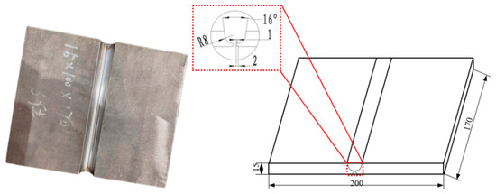
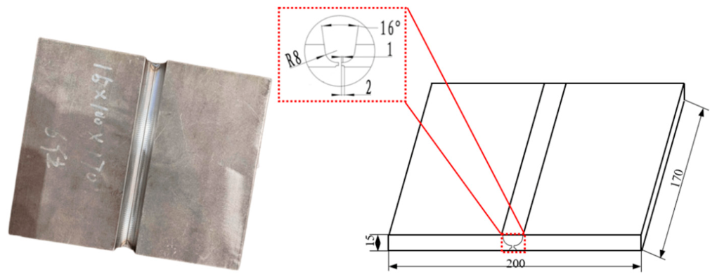
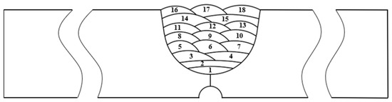
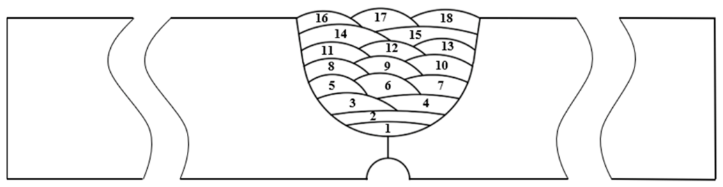
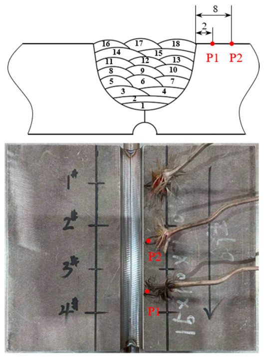
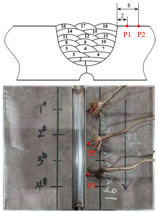
This study employed a 316LN stainless steel flat butt-welded joint with a nominal plate thickness of 15 mm. A plate thickness of 15 mm was selected for this study to ensure both experimental fidelity and practical feasibility. This thickness facilitates a rational stratified configuration and optimal weld seam arrangement, while enabling accurate numerical simulation of key welding thermomechanical phenomena—including heat input distribution, thermal cycling behavior, and progressive deformation evolution—observed in actual thick-section components. Furthermore, it mitigates the dimensional artifacts commonly associated with thin plates, thereby allowing faithful representation of the holistic thermomechanical response of the welded joint throughout the entire welding process. Balancing the need for result reliability against constraints on material usage and specimen fabrication cost, 15 mm represents an empirically justified and economically viable choice for the butt-welded joint configuration. A representative physical photograph and dimensional specifications prior to welding are presented in Figure 1. The joint groove configuration and sequential weld pass arrangement are detailed in Figure 2. To enable clear observation of root bead formation, a semi-circular concave groove (radius = 2 mm) was machined on the backside of the test plate; this feature was fully incorporated into the weld during fabrication. Manual argon arc welding was utilized as the primary joining process, with ER317L filler wire specifically selected for metallurgical compatibility with the 316LN base material. Inter-pass temperature was rigorously maintained below 100 °C throughout welding.

Figure 1. Shape and dimension of mock-up.

Figure 2. Welding sequence.

This study employs manual argon arc welding using a direct-current (DC) TIG welding system (Model YC-400TX4, Panasonic Industrial Company, Osaka, Japan). The machine’s rated operating parameters are as follows: nominal welding current range, 20–400 A; open-circuit voltage range, 20.8–36 V. The filler metal consists of ER317L stainless steel wire (diameter: 1.5 mm), and shielding is provided by high-purity argon gas (≥99.99% purity) delivered at a flow rate of 12 L/min. As illustrated in Figure 2, the butt-welded joint comprises 18 individual weld passes; the corresponding process parameters for each pass are tabulated in Table A1.

Thermal cycles at representative locations were recorded using NiCr-NiSi thermocouples coupled with a HiokiLR8431 data acquisition system (HIOKI E.E. Corporation, Ueda, Japan). Thermocouple placement is indicated in Figure 3: two sensors were positioned on the upper surface of the plate, at distances of 2 mm and 8 mm, respectively, from the groove edge.

Figure 3. Arrangement of thermocouple.

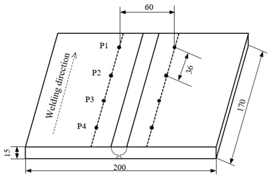
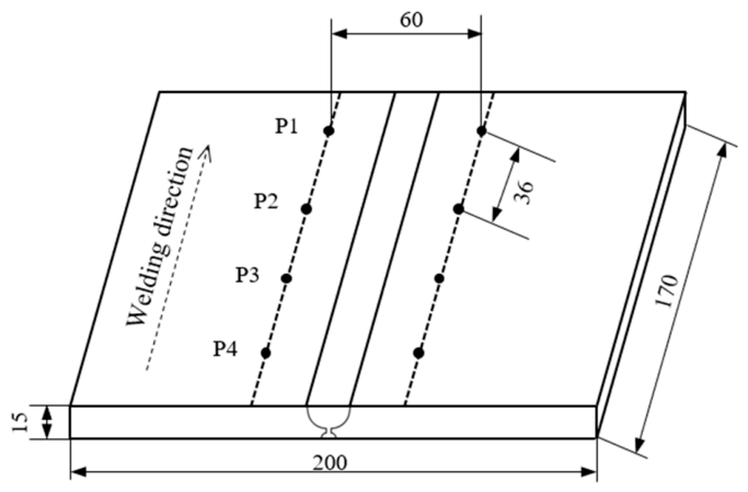
Post-weld geometric distortions including transverse shrinkage and angular distortion were quantified using a digital vernier caliper and a coordinate measuring machine (CMM). The angular distortion of the welded joint was measured using a G-80C coordinate measuring machine (CMM). Transverse shrinkage was quantified by determining the dimensional change—before and after welding—in the center-to-center distance between paired blind holes spaced 60 mm apart, as measured with a digital vernier caliper. The arrangement of these blind holes is illustrated in Figure 4.

Figure 4. Measurement position of transverse shrinkage. (unit: mm).

Subsequent to deformation assessment, residual stress distribution on the upper surface of the weld joint was determined via the incremental hole-drilling strain-gauge method. In this study, surface residual stresses in the welded joint were measured using the blind-hole drilling method, in strict accordance with the Chinese national standard GB/T 31310–2014 [28]. Measurements were conducted using an HK21A residual stress analyzer. A ZEMIC BE120-2CA-K foil strain gauge (nominal resistance: 120.3 ± 0.3 Ω, Zhonghang Electronic Measuring Instruments Co., Ltd., Xi’an, China) was employed for strain acquisition. The drilled blind hole had a diameter of 1.5 mm and a depth of 2.0 mm.

The calculation formula for residual stress by the hole-drilling method is as follows [29]:

$${\sigma }_{1,2}={\displaystyle \frac{{\epsilon }_1+{\epsilon }_2}{4A}}\pm {\displaystyle \frac{\sqrt{{\left({\epsilon }_1-{\epsilon }_3\right)}^2+{\left({2\epsilon }_2-{\epsilon }_1-{\epsilon }_3\right)}^2}}{4B}}$$

(1)

$$\tan 2\theta ={\displaystyle \frac{{\epsilon }_1+{\epsilon }_3-2{\epsilon }_2}{{\epsilon }_1-{\epsilon }_3}}$$

(2)

where ε₁, ε₂, and ε₃ represent the released strains in the reference direction, the direction at 45° to the reference direction, and the perpendicular direction, respectively; θ denotes the principal stress angle. The two release coefficients A and B are expressed as follows [29]:

$$A=-{\displaystyle \frac{1+\nu }{2E}}\left({\displaystyle \frac{d^2}{4r_1{r}_2}}\right)$$

(3)

$$B={\displaystyle \frac{d^2}{4{Er}_1{r}_2}}\left[-1+{\displaystyle \frac{1+\nu }{4}}·{\displaystyle \frac{d^2\left(r_1^2+r_1+r_2^2\right)}{4r_1^2{r}_2^2}}\right]$$

(4)

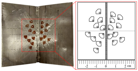
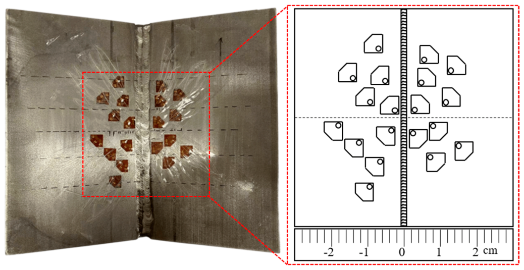
Based on preliminary finite element analysis, regions exhibiting elevated residual stress magnitudes and steep stress gradients were identified primarily within the weld metal, heat-affected zone (HAZ), and adjacent parent material. Consequently, strain gauges were strategically deployed in these high-gradient zones. Furthermore, because longitudinal and transverse residual stress variations along the weld axis are comparatively gradual in the central region of the test plate, strain gauges were arranged in a longitudinally dispersed configuration to minimize cross-talk and mutual interference among adjacent measurement points. The final strain gauge layout is depicted in Figure 5.

Figure 5. Schematic diagram of arrangement of strain gauge.

The experimentally obtained welding distortion and residual stress data serve two principal purposes: (i) direct characterization of distortion behavior and residual stress distribution in 316LN butt welds, and (ii) quantitative validation of the predictive accuracy of associated thermomechanical finite element simulations.

3. Methodology of Finite Element Simulation

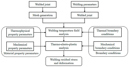
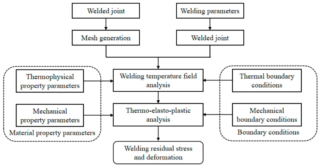
This study employs a thermal–mechanical coupled finite element modeling approach, implemented within the MSC. Marc 2020 software environment, to simulate the transient temperature field and residual stress distribution and welding-induced deformation during multi-pass butt welding of 316LN stainless steel. The computational workflow is illustrated in Figure 6.

Figure 6. Flowchart of thermo-elastic–plastic analysis procedure.

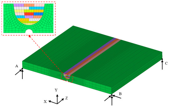
A three-dimensional finite element mesh was constructed to faithfully represent the actual joint geometry, including weld bead dimensions and pass deposition order—all strictly aligned with the experimental welding procedure. Mesh refinement was strategically applied in regions exhibiting steep thermal gradients, high stress gradients, and significant plastic strain accumulation—namely, the weld metal, heat-affected zone (HAZ), and adjacent base metal—while coarser discretization was employed in thermomechanically inactive regions distant from the weld zone. This adaptive meshing strategy ensures an optimal balance between computational accuracy and efficiency. The computational mesh for the butt-welded joint consists of 83,200 hexahedral elements and 91,203 nodes (Figure 7). For thermal analysis, MSC. Marc software’s built-in 43rd element type was adopted, and the 7th element type was used in the stress–strain calculation process [30]. Both the 43rd element and 7th element are 8-node hexahedral elements. The 43rd element has temperature degrees of freedom and can be used for thermal analysis, while the 7th element has no temperature degrees of freedom and is applicable for the calculation of welding stress and deformation.

Figure 7. Finite element mesh model and arrangement of weld passes.

In the thermal analysis phase, internal heat source models were employed to characterize the spatial and temporal distribution of arc energy inputs. Concurrently, convective and radiative heat losses across all six external surfaces were explicitly modeled: convection is governed by Newton’s law of cooling, while radiation follows the Stefan–Boltzmann law. Transient heat conduction within the workpiece was solved using the Fourier heat equation, incorporating temperature-dependent thermophysical properties—including density, specific heat capacity, and thermal conductivity.

The resulting time-resolved nodal temperature history serves as the thermal loading input for the subsequent mechanical analysis. In this stage, temperature-dependent elastic–plastic constitutive behavior was implemented, accounting for thermal expansion, yield strength softening, and isotropic hardening/annealing evolution. Mechanical boundary conditions replicated those of the free-standing experimental setup: no external restraints were imposed, except for minimal kinematic constraints necessary to suppress rigid-body motion. Specifically, a “three-point, six-degree-of-freedom” constraint scheme was applied at nodes A, B, and C (Figure 7), thereby eliminating translation and rotation without introducing artificial reaction forces or stress artifacts.

The primary objective of this section was to establish a robust, experimentally grounded simulation methodology prior to systematically evaluating the sensitivity of residual stress and distortion predictions to alternative heat source formulations. Section 3.1 presents a comparative assessment of three distinct heat source models, with emphasis on both predictive fidelity and computational efficiency.

3.1. Welding Heat Source Modeling

The thermal–mechanical coupling behavior inherent in welding processes constitutes a strongly nonlinear problem. Despite substantial advances in computational hardware, numerical simulation of welding—particularly for large-scale, geometrically complex, or thick-section structures—remains computationally demanding. A critical challenge therefore lies in devising an appropriate modeling strategy that achieves an optimal trade-off between computational efficiency and solution fidelity. To enhance the computational efficiency of thermal elastic–plastic simulations in welding, potential avenues include algorithmic optimization, hardware-accelerated computing, and judicious model simplification. Among these, the selection of a physically appropriate heat source model—tailored to both the specific weld configuration and the intended simulation objectives—represents a practical and effective approach. This study comparatively evaluates three representative heat source formulations: the instantaneous heat source, the enhanced moving heat source, and the moving element-set heat source model. Their respective influences on residual stress development and distortion in a multi-pass butt-welded joint of 15 mm thick 316LN stainless steel were systematically investigated. The findings will provide methodological guidance for selecting suitable heat source models in subsequent numerical analyses of engineering-scale welding applications. These three models are introduced sequentially below: the instantaneous heat source, the enhanced moving heat source, and the moving element-set heat source model.

3.1.1. Instantaneous Heat Source Model

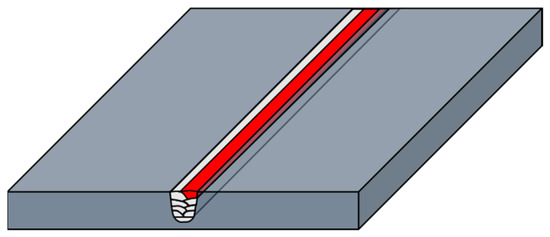
The instantaneous heat source model is a computationally efficient simplification that assumes uniform, simultaneous heating along the entire weld seam—without explicitly resolving temporal progression of the arc along the welding direction. In multi-layer, multi-pass welding simulations, this formulation reduces the transient three-dimensional heat conduction problem to a quasi-steady two-dimensional one, thereby significantly decreasing computational cost. Likewise, in mechanical analysis, it obviates the need for numerous small time increments (as required by moving-source formulations), substantially accelerating convergence. The specific implementation adopted herein is illustrated in Figure 8, and the red line in this figure denotes the last weld pass, indicating that the entire pass is subjected to uniform and simultaneous heating.

Figure 8. Schematic diagram of instantaneous heat source.

It is important to emphasize that although the instantaneous model neglects arc motion kinematics, the total volumetric heat input per pass is rigorously preserved and fully consistent with experimentally determined welding parameters. Consequently, two key parameters must be carefully calibrated: the spatially distributed heat flux density (q) and the effective heating duration (tₕ). Given fixed weld bead geometry and total heat input, appropriate pairing of q and tₕ enables realistic prediction of melt pool morphology, as well as accurate estimation of both average and peak temperatures within the fusion zone.

The nominal heat input per weld pass is derived from fundamental welding parameters—namely, arc voltage (U), welding current (I), and nominal pass duration (t)—according to standard practice. Accounting for arc thermal efficiency (η), the net heat input Q is computed via Equation (5):

$$Q=\eta UIt$$

(5)

For tungsten inert gas (TIG) welding, η is typically taken as 0.7.

The nominal pass duration t is determined by weld seam length (L) and travel speed (v), as expressed in Equation (6):

$$t={\displaystyle \raisebox{1ex}{$L$}\!\left/ \!\raisebox{-1ex}{$v$}\right.}$$

(6)

Once the volume V of each weld bead is established, the heat flux density q for the instantaneous model is calculated using Equation (7):

$$q={\displaystyle \frac{Q}{\left(V·t_h\right)}}$$

(7)

Here, t_h denotes the effective heating time—a parameter representing the duration over which heat is uniformly applied across the entire weld pass. Empirical evidence suggests t_h typically falls within the range of 2–6 s; in this study, t_h is conservatively set to 3 s.

3.1.2. Enhanced Moving Heat Source Model

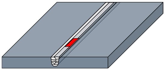
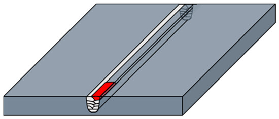
In this study, we attempted to propose a heat source model that lies between the instantaneous heat source and the moving heat source. This heat source model is similar to the aforementioned moving heat source model, except that we artificially increase the length of the heat source model to three times its original length. Thus, compared to the above moving heat source, it can improve the computational efficiency to a certain extent. The schematic diagram of the enhanced moving heat source is shown in Figure 9, and the red region in the figure denotes the spatial extent of the enhanced moving heat source.

Figure 9. Schematic diagram of enhanced moving heat source.

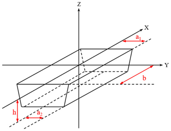
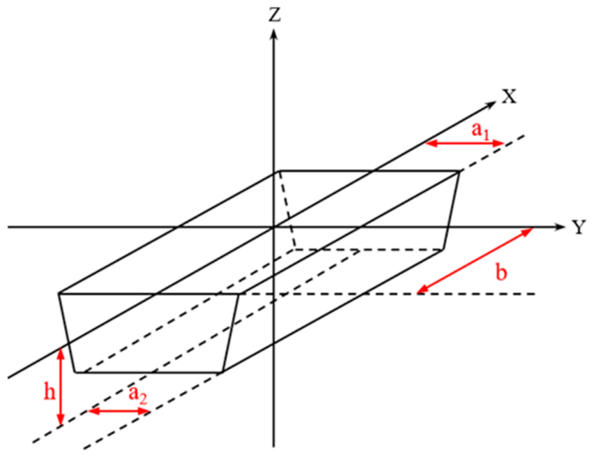
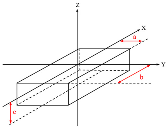
The enhanced moving heat source used in this study is a trapezoidal heat source, as shown in Figure 10. The range of this heat source can be described by Equation (8):

$$\left\{\begin{array}{c}\left|x-vt\right|\le b\\ -h\le z\le 0\\ \left|{\displaystyle \frac{h}{a_2-a_1}}\right|y+{\displaystyle \frac{a_{1}h}{a_2-a_1}}\le z\end{array}\right.$$

(8)

where a₁ and a₂ are half the length of the upper and lower base of the heat source, b is the half-length of the heat source, h is the height of the heat source, v is the welding speed, and t is the welding time.

Figure 10. Enhanced moving heat source.

The volume V of the heat source and the heat flux density q_v1 are described by Equations (9) and (10) respectively:

$$V=2bh·\left(a_1+a_2\right)$$

(9)

$$q_{v1}={\displaystyle \frac{\eta Q}{V}}$$

(10)

where Q is the heat input of the heat source, and η is the heat efficiency, assumed in this study to be 0.7.

3.1.3. Moving Element-Set Heat Source Model

When simulating the temperature field of a multi-pass welded joint, the traditional approach is to load all the elements covered by the current weld pass into the finite element model, and then use a moving heat source model such as the classic Gaussian double-ellipsoid heat source model to simulate the welding arc movement process. Usually, subroutines are needed to define heat source parameters, the center position of the heat source, welding parameters, etc.

Multi-pass welding is characterized by many weld beads. When using the traditional double-ellipsoid moving heat source model, it is difficult to control the pool morphology and it is difficult to achieve precise matching of heat input and pool morphology. Therefore, when studying multi-pass welding problems, a volume heat source with uniform density in the element shape can be adopted. When using this heat source model, the size of the weld pass section is defined based on the position of each weld pass and the heat input, and after defining an appropriate length, the range of the heat source can be obtained. Of course, the size of the weld pass section can also be defined by referring to the metallographic images after welding. This approach is more physically based, but it is more cumbersome.

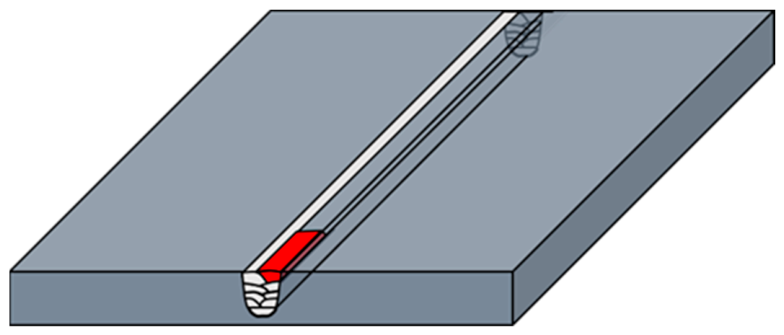
To consider the influence of the transient process of weld pass filling on the temperature field and stress in detail, this study has developed a special equal-density heat source model, called the moving element-set heat source model. In this model, a user subroutine is used to control the simulation of the welding material melting process by the elements involved in the weld pass; that is, the elements at the location where the heat source moves to are activated when the heat source reaches the current position of the weld pass. The schematic diagram is shown in Figure 11, and the red region in the figure denotes the spatial extent of moving element-set heat source.

Figure 11. Schematic diagram of moving element-set heat source model.

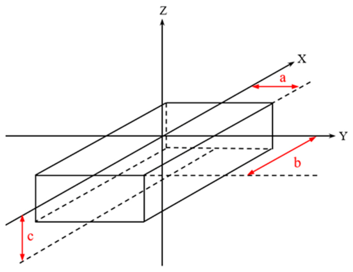
The moving element-set heat source used in this study is a rectangular equal-density heat source, as shown in Figure 12. The range of the heat source can be described by Equation (11):

$$\left\{\begin{array}{c}\left|x-vt\right|\le b\\ -c\le z\le 0\\ \left|y\right|\le a\end{array}\right.$$

(11)

where a and b are the half-width and half-length of the heat source, c is the height of the heat source, v is the welding speed, and t is the welding time.

Figure 12. Moving element-set heat source.

The volume V and the heat flux density q_v of the heat source are described by Equations (12) and (13):

$$V=4abc$$

(12)

$$q_v={\displaystyle \frac{\eta Q}{V}}$$

(13)

3.2. Analysis of Welding Temperature Field

A transient, nonlinear heat transfer analysis was employed to model the welding thermal process. The governing equation for Fourier’s law of heat conduction—assuming isotropic and temperature-dependent thermal conductivity—is expressed as follows [31]:

$$q=-k\nabla T$$

(14)

where q denotes the heat flux vector (W·mm⁻²), and k represents the thermal conductivity (W·mm⁻¹·°C⁻¹), which may vary with temperature.

The evolution of nodal thermal cycles and the spatial temporal distribution of the temperature field were obtained via finite element simulation. These results satisfy the general energy conservation equation for transient heat conduction [31]:

$$\rho c_p{\displaystyle \frac{\mathit{\partial }T}{\mathit{\partial }t}}\left(x,y,z,t\right)=-\nabla q\left(x,y,z,t\right)+Q_v\left(x,y,z,t\right)$$

(15)

where ρ is the material density (g·mm⁻³); c_p is the specific heat capacity (J·g⁻¹·°C⁻¹); T is the instantaneous temperature (°C); Q_v denotes the volumetric internal heat generation rate (W·mm⁻³); t is the physical time (s); and ∇ is the Laplacian operator in Cartesian coordinates, with x, y, and z representing the spatial coordinates (mm) in the global reference frame.

In addition to conductive heat transfer within the welded plate, boundary heat exchange with the ambient environment including convection and radiation was explicitly incorporated. Convective heat loss at the plate surface follows Newton’s law of cooling (Equation (16) [31,32]):

$$q_c=-h\left(T_s-T_a\right)$$

(16)

where h is the convective heat transfer coefficient (2 × 10⁻⁵ W·mm⁻²·°C⁻¹), T_s is the local surface temperature (°C), and Tₐ is the ambient temperature (20 °C).

Radiative heat loss was modeled using the Stefan–Boltzmann law (Equation (17) [31]):

$$q_r=-\epsilon \sigma \left[{\left(T_s+273\right)}^4-{\left(T_a+273\right)}^4\right]$$

(17)

where ε is the surface emissivity (assumed constant at 0.8), and σ is the Stefan–Boltzmann constant (5.67 × 10⁻¹⁴ W·mm⁻²·K⁻⁴).

To ensure computational efficiency and numerical stability, heat exchange between the welded component and its fixtures or assembly supports was omitted. This simplification is justified by prior validation studies indicating negligible influence on predicted welding-induced deformations, while substantially reducing computational cost and enhancing solution convergence.

3.3. Analysis of Welding Stress and Strain

The temperature distribution obtained from the thermal analysis serves as the thermal loading condition for subsequent structural analysis. A thermo-elastic–plastic finite element simulation was performed to predict residual stresses and welding-induced distortions. During welding, the total strain tensor of the material can be decomposed into constituent components as expressed in Equation (18):

$$\epsilon ={\epsilon }^e+{\epsilon }^p+{\epsilon }^t+{\epsilon }^{ph}+{\epsilon }^c$$

(18)

where ε^e denotes elastic strain; ε^p, plastic strain; ε^t, thermal strain; ε^ph, phase transformation strain; and ε^c, creep strain.

Given the transient nature of the welding thermal cycle—characterized by rapid heating and cooling—the duration of elevated temperatures is insufficient to induce significant creep deformation. Consequently, the creep strain component (ε^c) was omitted from the constitutive formulation. Furthermore, the 316LN austenitic stainless steel employed in this study exhibits a stable single-phase austenitic microstructure across the entire thermal cycle, with no solid-state phase transformations occurring during heating or cooling. Hence, the phase transformation strain term (ε^ph) was also excluded. As a result, the strain–stress relationship adopted in the mechanical analysis simplifies to Equation (19):

$$\epsilon ={\epsilon }^e+{\epsilon }^p+{\epsilon }^t$$

(19)

The elastic response is modeled using isotropic Hooke’s law. Under the generalized form of Hooke’s law, the relationships between normal strains, shear strains, and corresponding stress components are given by Equations (20) and (21), respectively:

$$\left\{\begin{array}{c}{\epsilon }_x={\displaystyle \frac{1}{E}}\left[{\sigma }_x-v\left({\sigma }_y+{\sigma }_z\right)\right]\\ {\epsilon }_y={\displaystyle \frac{1}{E}}\left[{\sigma }_y-v\left({\sigma }_x+{\sigma }_z\right)\right]\\ {\epsilon }_z={\displaystyle \frac{1}{E}}\left[{\sigma }_z-v\left({\sigma }_x+{\sigma }_y\right)\right]\end{array}\right.$$

(20)

$${\mathsf{{\rm Y}}}_{xy}={\displaystyle \frac{{\tau }_{xy}}{G}}, {\mathsf{{\rm Y}}}_{yz}={\displaystyle \frac{{\tau }_{yz}}{G}},{\mathsf{{\rm Y}}}_{zx}={\displaystyle \frac{{\tau }_{zx}}{G}}$$

(21)

where E denotes Young’s modulus; ν, Poisson’s ratio; τ_xy, τ_yz, τ_zx, shear stress; and G, the shear modulus (G = E/[2(1 + ν)]).

In the mechanical model, plastic deformation is governed by the von Mises yield criterion. Owing to the pronounced work-hardening behavior of 316LN stainless steel, the isotropic hardening was adopted to capture the evolution of the yield surface. A full annealing temperature of 900 °C is prescribed: upon reaching this temperature, the accumulated equivalent plastic strain is reset to zero to reflect microstructural recovery.

Numerical accuracy in welding simulation depends critically on three interrelated factors: (i) a physically representative constitutive model, (ii) well-defined boundary and loading conditions, and (iii) temperature-dependent material properties. In particular, thermal–physical and mechanical parameters including thermal conductivity, specific heat, coefficient of thermal expansion, Young’s modulus, yield strength, and hardening behavior must be specified as continuous functions of temperature.

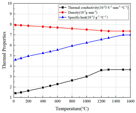
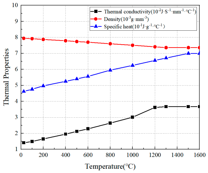
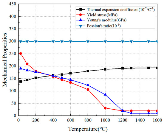
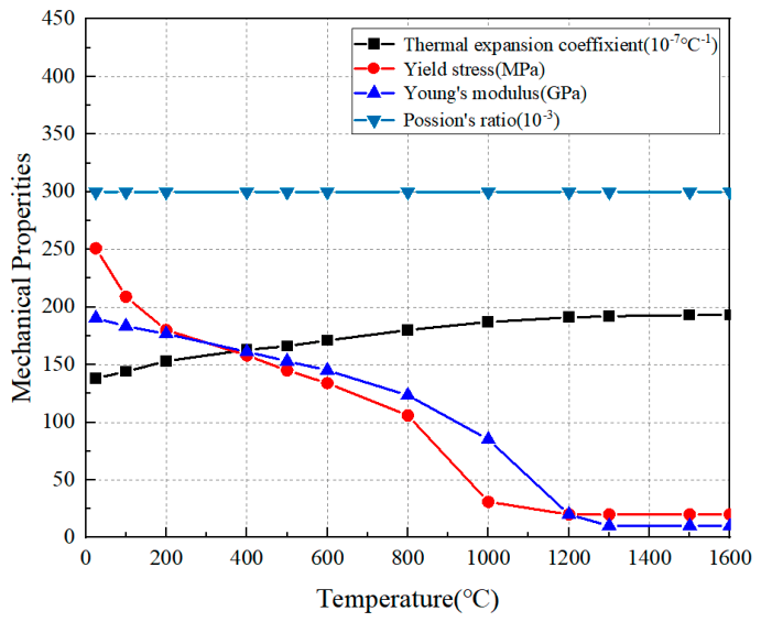
In this study, the specific heat capacity, thermal conductivity, and density of 316LN austenitic stainless steel were experimentally determined over the temperature range of 25 °C to 1000 °C using a laser flash apparatus (NETZSCH LFA 467 HT, NETZSCH-Gerätebau GmbH, Selb, Germany). For temperatures exceeding 1000 °C—up to the metallurgical melting point—the same thermophysical properties were estimated via thermodynamic modeling using JMatPro software (version 7.0), based on the nominal chemical composition of the alloy. Uniaxial tensile tests were conducted from 25 °C to 1000 °C using an electronic universal testing machine (WDW-3100, Changchun Kexin Test Instrument Co., Ltd., Changchun, China), with specimens fabricated in strict accordance with the GB/T 228.1–2021 standard [33] for metallic materials. A constant crosshead displacement rate of 2 mm/min was employed, and axial strain was measured directly using a calibrated extensometer. Yield strength and elastic modulus were extracted from the resulting stress–strain curves at each test temperature. For temperatures between 1000 °C and the melting point, these mechanical parameters were likewise predicted using JMatPro (version 7.0). A constant Poisson’s ratio of 0.3 was adopted throughout the analysis, consistent with established literature values for austenitic stainless steels under elevated-temperature conditions.

The performance parameters of 316LN austenitic stainless steel obtained by test and calculation are shown in Figure 13 and Figure 14. Given the compositional and mechanical similarity between the weld metal and base metal, identical temperature-dependent property curves are assigned to both regions in the finite element model.

Figure 13. Temperature-dependent thermal–physical properties of 316LN austenitic stainless steel.

Figure 14. Temperature-dependent mechanical properties of 316LN austenitic stainless steel.

3.4. Simulation Cases

To systematically evaluate the influence of heat source modeling on predicted weld pool geometry, residual stress distribution, and distortion in the multi-pass butt-welded 316LN joint, three distinct simulation cases were formulated, as detailed in Table 1. All cases share identical mesh topology, element type, and discretization density—differing solely in the mathematical representation of the heat source. Notably, for improved computational efficiency—particularly in the instantaneous heat source simulation—the mesh density along the welding direction may be coarsened without compromising solution fidelity, provided that key thermal and mechanical gradients remain adequately resolved. All simulations were executed on identical hardware: an AMD Ryzen 9 9950X CPU (base frequency 4.3 GHz), equipped with 128 GB of DDR5 RAM.

Table 1. Simulation cases.

Cases	Heat Source Model
Case 1	Instantaneous Heat Source Model
Case 2	Enhanced Moving Heat Source Model
Case 3	Moving Element-Set Heat Source Model

4. Results and Discussion

4.1. Results of Welding Temperature Field

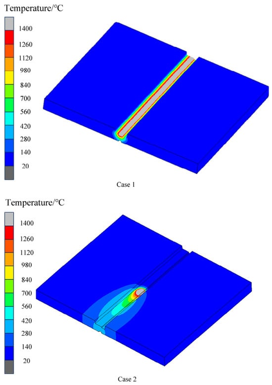
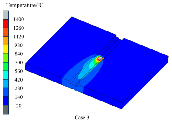
First, the temperature field distribution characteristics of the three heat source models—namely, the instantaneous heat source, the enhanced moving heat source, and the moving element-set heat source—are comparatively analyzed during the welding heating phase. For illustrative purposes, the temperature field corresponding to the ninth weld pass is selected as the representative case. As shown in Figure 15, the simulated temperature fields exhibit notable differences in temperature distribution; however, the predicted molten pool widths remain largely consistent across all three models. Case 1 employed the instantaneous heat source model, yielding a uniform, strip-shaped temperature distribution across the entire weld zone. The entire weld region reached the melting temperature, resulting in a continuous molten zone; the corresponding temperature field exhibited predominantly two-dimensional (2D) characteristics. In contrast, Case 2 utilized an enhanced moving heat source model, producing a distinctly three-dimensional (3D) temperature field. A steep temperature gradient was observed near the leading edge of the heat source, whereas the gradient at the trailing edge was comparatively gradual. Case 3 applied the moving element-set heat source model, which generated a significantly smaller molten pool than that in Case 2 and accentuated the 3D nature of the temperature distribution. Although the longitudinal temperature field profiles differed markedly among the three heat source models, the resulting weld geometry—including width, depth, and overall dimensions—as well as the transverse temperature gradients remained largely consistent.

Figure 15. Temperature field distribution of the 9th welding pass.

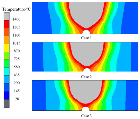
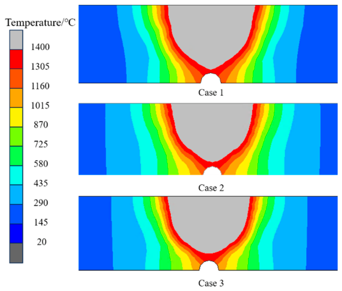
Figure 16 presents the peak temperature distribution along the middle cross-section of the joint after completion of welding. The melting zones—defined as regions where temperature exceeds the metallurgical melting point of approximately 1400 °C for both 316LN stainless steel base metal and weld metal—are highlighted in gray. Quantitative comparison reveals that the shapes and areas of the predicted melting zones are highly similar among the three models, although the moving element-set heat source yields marginally narrower melting zones relative to the instantaneous heat source and the enhanced moving heat source.

Figure 16. Contour plot of cross-sectional peak temperature distribution.

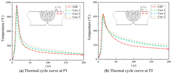
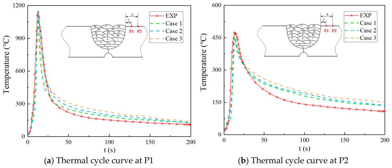
To enable quantitative assessment of thermal behavior under differing heat source assumptions, welding thermal cycles at two representative locations—P1 and P2—during the final (18th) weld pass are examined. Both numerically simulated and experimentally measured thermal cycles are presented in Figure 17. At location P1 (Figure 17a), the simulated and measured peak temperatures converge at approximately 1150 °C. During the heating phase and subsequent cooling down to 400 °C, all three simulation cases demonstrate strong agreement with experimental data. However, discrepancies emerge during the low-temperature cooling regime (<400 °C), wherein the measured cooling rates exceed those predicted numerically. This deviation is attributed primarily to two modeling simplifications: (i) omission of conductive heat transfer between the welded component and the supporting fixture (e.g., workbench pad) in the finite element thermal boundary condition setup; and (ii) adoption of a constant convective heat transfer coefficient, neglecting its experimentally observed temperature dependence. Given that 316LN is an austenitic stainless steel exhibiting no solid-state phase transformations upon cooling, such minor discrepancies in low-temperature cooling kinetics exert only limited influence on the predicted welding-induced distortion and residual stress distribution. Similarly, at location P2 (Figure 17b), excellent agreement between simulation and measurement is observed during heating and initial cooling; however, measured cooling rates again surpass simulated values below 300 °C. Furthermore, comparative analysis of Figure 17 indicates a systematic trend in predicted cooling kinetics: the moving element-set heat source yields the slowest cooling rate, whereas the instantaneous heat source predicts the fastest cooling rate.

Figure 17. Thermal cycles of typical position in welded joint.

4.2. Welding Residual Stress Results

4.2.1. Longitudinal Residual Stress

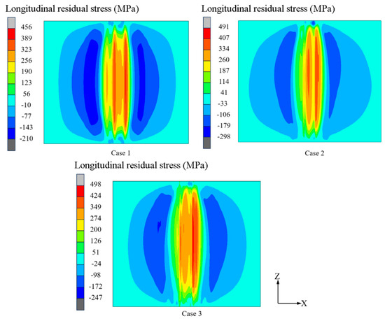
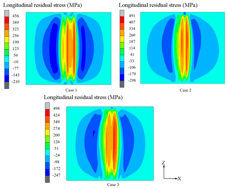
Figure 18 presents the numerically predicted longitudinal residual stress distributions on the upper surface of the welded joint, obtained using three distinct heat source models: the instantaneous heat source (case 1), enhanced moving heat source (case 2), and the moving element-set heat source (case 3). Overall, the spatial distribution patterns of longitudinal residual stress predicted by all three models exhibit strong qualitative agreement. However, quantitative and morphological differences arise due to their underlying assumptions regarding heat input dynamics. Specifically, the instantaneous heat source model neglects arc travel effects and assumes uniform heating across the entire weld pass; consequently, it yields symmetric stress distributions near both the start and end regions of the butt-welded joint. In contrast, both moving heat source models—by explicitly incorporating arc motion—capture asymmetry in the stress field, reflecting the transient thermal–mechanical history during welding.

Figure 18. Contours of longitudinal residual stress distribution.

Peak longitudinal residual stress values are quantified as follows: 456 MPa for the instantaneous heat source, 491 MPa for the enhanced moving heat source, and 498 MPa for the moving element-set heat source. These incremental increases reflect progressively more realistic representations of localized thermal loading and associated longitudinal restraint. The elevated peak for the moving element-set heat source arises from its relatively concentrated thermal profile and stronger local constraint during arc progression, whereas the instantaneous model’s lower peak stems from simultaneous heating of the full weld length at elevated temperatures—wherein the temperature-dependent reduction in elastic modulus attenuates internal longitudinal restraint within the weld pass.

Notably, all three models predict peak longitudinal tensile residual stresses significantly exceeding the material’s room-temperature yield strength (265 MPa). This behavior is consistent with established metallurgical and mechanical mechanisms in multi-pass, medium-to-thick-plate welding: (i) strain hardening induced by successive thermal cycles and plastic deformation accumulation, and (ii) pronounced multiaxial stress states arising from geometric constraints—particularly in the through-thickness direction—which elevate the effective stress component along the longitudinal axis beyond the uniaxial yield limit. Such stress levels are characteristic of residual stress fields in structural thick-section weldments.

Figure 19 further compares the longitudinal residual stress distributions along the central cross-section. All models reproduce a common high-tensile zone located at two key locations: (i) the attachment region of the final facing pass, where subsequent weld passes impose substantial mechanical restraint, and (ii) the groove root on the lower surface of the test plate, where geometric discontinuity induces stress concentration.

Figure 19. Contour plot of longitudinal residual stress distribution through the plate thickness.

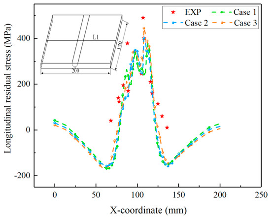
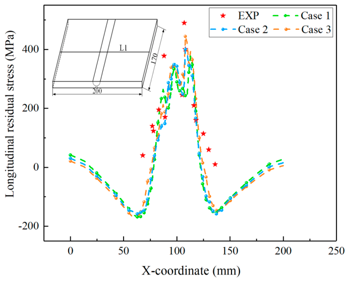
Figure 20 plots the longitudinal residual stress profiles along line L1 (upper surface) for all three simulations alongside experimental measurements. The predicted curves demonstrate excellent shape fidelity and strong quantitative agreement with measured data. In particular, an “M-shaped” distribution is consistently observed in the weld-proximal region, with the dominant peak situated to the right of the final weld pass attachment. A detailed comparison reveals that the moving element-set heat source model yields the highest predicted stress magnitude along L1 and exhibits the closest alignment with experimental values—indicating superior predictive capability among the three approaches under the given boundary and material assumptions.

Figure 20. Distribution of longitudinal residual stress along L1.

Collectively, the comparative analysis demonstrates that even the simplified instantaneous heat source model can deliver acceptable accuracy for longitudinal residual stress prediction in this configuration. Nevertheless, the moving element-set heat source model provides the most balanced trade-off between computational efficiency and fidelity, particularly when capturing localized stress gradients and quantitative agreement with experimental validation data.

4.2.2. Transverse Residual Stress

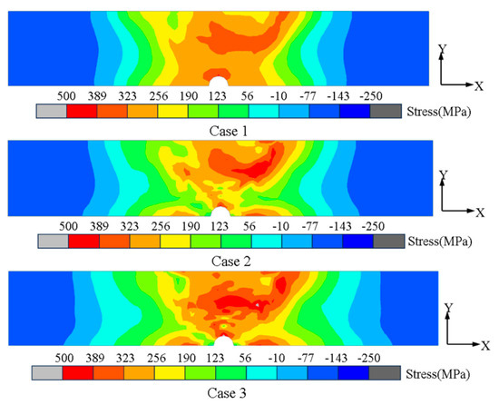
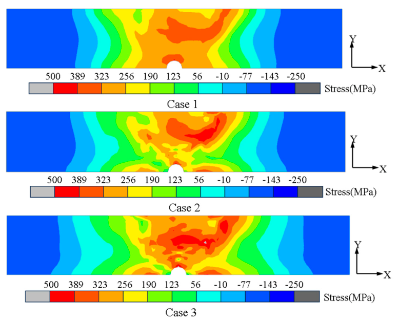
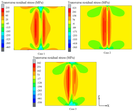
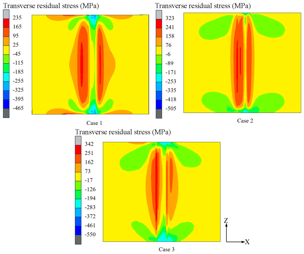
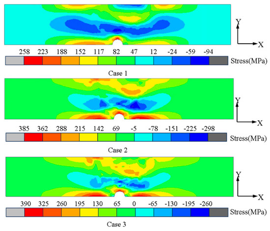
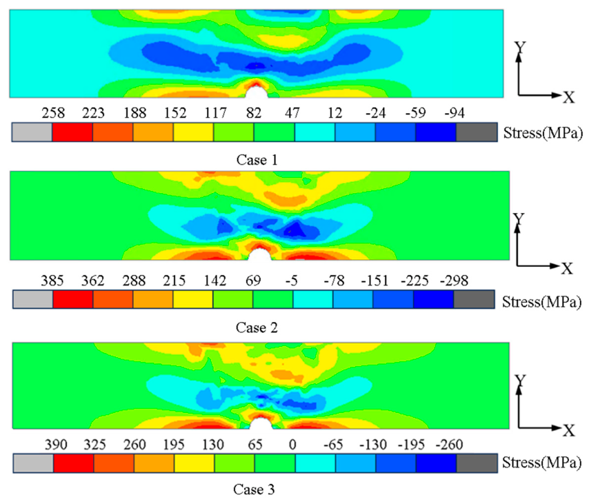
Figure 21 presents the numerically predicted the contour distributions of transverse residual stress, obtained using instantaneous heat source (case 1), enhanced moving heat source (case 2), and moving element-set heat source (case 3) models, respectively. Overall, the three models yield qualitatively similar residual stress patterns. However, a detailed comparative analysis reveals notable quantitative discrepancies. Specifically, the IHS model predicts a distinct spatial distribution of tensile residual stress near the butt-welded joint ends—deviating from the distributions obtained with the MHS and EMHS models. Moreover, the peak tensile residual stress predicted by the IHS model is substantially lower (by approximately 34% relative to the MHS result), indicating that residual stress predictions are highly sensitive to the choice of heat source formulation. As previously discussed, the IHS model inherently underestimates thermal–mechanical restraint in the transverse direction compared with actual welding conditions. This reduced restraint leads to attenuated plastic strain magnitudes and altered plastic strain distributions, which in turn influence the magnitude and spatial profile of the associated elastic strain—directly governing the resulting residual stress field.

Figure 21. Contours of transverse residual stress.

Figure 22 illustrates the transverse residual stress distributions across the middle cross-section of the test plate for the three modeling approaches. A more pronounced divergence emerges in this region: the IHS model (case 1) yields a broader zone of compressive residual stress and exhibits a markedly different stress gradient profile compared with the EMHS (case 2) and MHS (case 3) results. Quantitatively, the peak transverse tensile residual stresses predicted by the IHS, EMHS, and MHS models are 258 MPa, 385 MPa, and 390 MPa, respectively—corresponding to a maximum inter-model deviation of ~140 MPa (≈36% relative to the IHS value). This confirms that the IHS model systematically underestimates the magnitude of transverse tensile residual stress.

Figure 22. Contour plot of transverse residual stress distribution through the plate thickness.

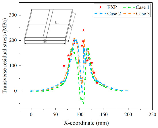
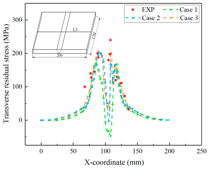
Figure 23 compares the transverse residual stress distributions along line L1 (upper surface) for all three models, overlaid with experimentally measured data. All three simulations reproduce the general trend of the measured distribution; however, the MHS prediction demonstrates the closest agreement with experimental values, whereas the IHS prediction consistently underestimates stress levels—particularly in the high-stress regions adjacent to the weld centerline. Notably, the peak transverse tensile residual stress remains well below the material’s yield strength across all cases. Consequently, when moderate accuracy suffices for transverse residual stress assessment—especially in preliminary design or parametric studies—the IHS model may serve as a computationally efficient alternative, offering acceptable fidelity for longitudinal residual stress prediction and a reasonably representative transverse stress distribution. This trade-off between computational efficiency and predictive accuracy holds practical relevance for engineering applications involving large-scale structural simulation.

Figure 23. Distribution of transverse residual stress along L1.

4.3. Welding Deformation Results

4.3.1. Angular Distortion

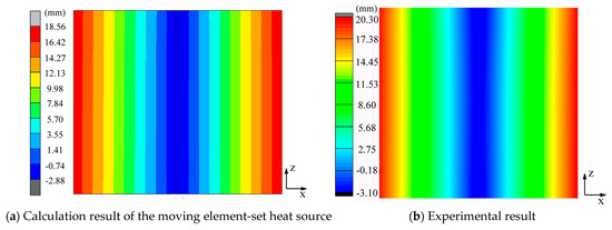
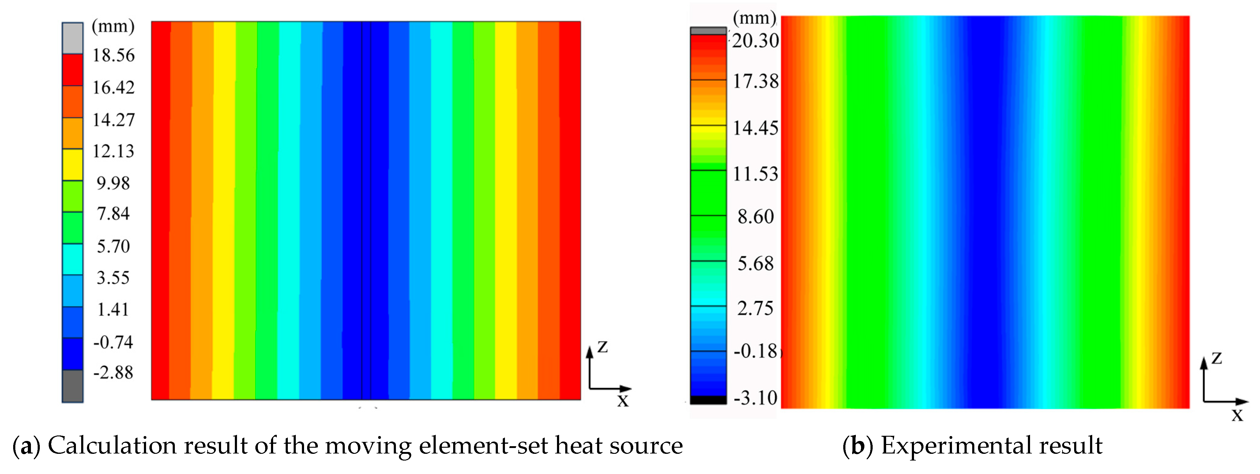
Figure 24 compares the out-of-plane angular distortion predicted by the moving element-set heat source model with corresponding experimental measurements: Figure 24a displays the simulated deformation profile, while Figure 24b shows the experimentally obtained counterpart. All cases display a symmetric distribution of deformation with respect to the weld centerline, with maximum deformation occurring at the base metal edges adjacent to the weld on both sides, and minimum deformation observed at the weld center. Quantitatively, the measured angular deformation is 23.40 mm, whereas the simulation yields 21.42 mm, resulting in a relative error of 8.5% and an agreement level exceeding 90%.

Figure 24. Angular distortion of butt-welded joint.

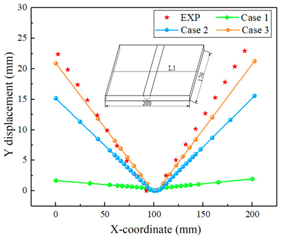
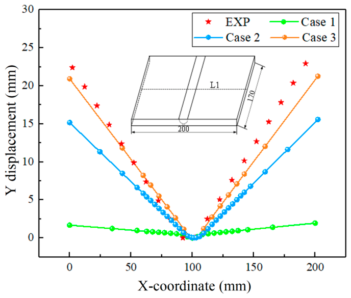
Figure 25 illustrates the angular deformation distribution along the central cross-section, as predicted by the three thermal models, alongside the experimental reference data. As shown, the predicted angular deformations increase progressively across the models: 1.97 mm (instantaneous heat source), 15.16 mm (enhanced moving heat source), and 21.42 mm (moving element-set heat source). The error metrics between the angular distortion results obtained from experiments and simulations are quantified, as shown in Table 2. Relative to the experimental value of 23.40 mm, the instantaneous heat source exhibits a substantial discrepancy—yielding only 8.4% prediction accuracy—whereas the enhanced moving heat source achieves 64.8% accuracy. These results indicate that the moving element-set heat source model provides the most reliable prediction of angular deformation among the three formulations.

Figure 25. Angular deformation along line L1.

Table 2. Comparison of angular distortion results between experiment and simulations.

Cases	Heat Source Model	Angular Distortion Results	Degree of Conformity
Case 1	Instantaneous Heat Source Model	1.97 mm	8.42%
Case 2	Enhanced Moving Heat Source Model	15.16 mm	64.79%
Case 3	Moving Element-Set Heat Source Model	21.42 mm	91.54%
Experiment	-	23.40 mm	100%

Collectively, the analysis demonstrates that although the instantaneous heat source model may yield acceptable estimates of residual stress distribution, its capacity to predict geometric distortion—particularly angular deformation—is fundamentally limited.

4.3.2. Transverse Shrinkage

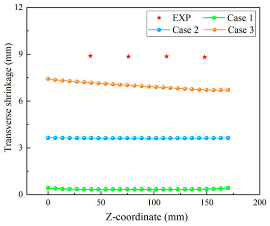
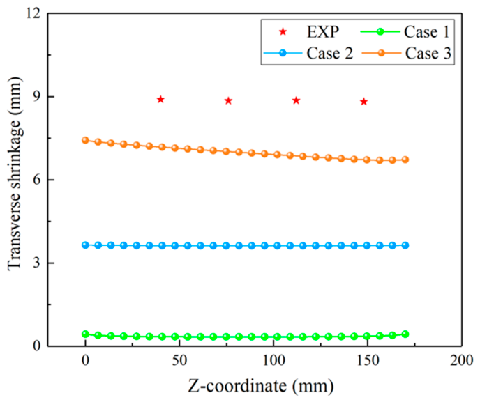
Figure 26 presents the transverse contraction distribution along the upper surface of the butt-welded joint, comparing predictions from the three thermal models against experimental measurements. The simulated values are 0.61 mm (instantaneous), 4.65 mm (enhanced moving), and 7.9 mm (moving element-set heat source), respectively—exhibiting the same monotonic trend observed for angular deformation. The error metrics between the transverse shrinkage results obtained from experiment and simulations are quantified, as shown in Table 3. Notably, the spatially averaged transverse contraction predicted by the moving element-set heat source model is 7.3 mm, which deviates from the experimental mean of 8.7 mm by approximately 16.1%.

Figure 26. Transverse displacement of the top surface along the longitudinal direction.

Table 3. Comparison of transverse shrinkage results between experiment and simulations.

Cases	Heat Source Model	Transverse Shrinkage Results	Degree of Conformity
Case 1	Instantaneous Heat Source Model	0.61 mm	7.01%
Case 2	Enhanced Moving Heat Source Model	4.65 mm	53.45%
Case 3	Moving Element-Set Heat Source Model	7.90 mm	90.80%
Experiment	-	8.70 mm	100%

Several factors likely contribute to this residual discrepancy. First, the initial root gap was not explicitly incorporated into the numerical model. Second, inter-pass temperatures and total heat input in the physical welding process may differ from those prescribed in the simulation. Third, uncertainties in temperature-dependent material properties—including thermal expansion, conductivity, and plastic flow behavior—inevitably affect the fidelity of thermomechanical predictions.

Consistent with the findings for angular deformation, Figure 26 reaffirms that the instantaneous heat source model is inadequate for predicting macroscopic welding distortion, despite its potential utility in residual stress assessment.

Furthermore, for the 15 mm thick 316LN stainless steel multi-layer, multi-pass butt-welded joint under investigation, the experimentally measured transverse contraction reaches 9.0 mm—significantly exceeding that observed in comparably thick low-alloy high-strength steel joints. This disparity arises primarily from two intrinsic material characteristics: (i) the coefficient of thermal expansion of 316LN is approximately 33% higher than that of low-alloy high-strength steels; and (ii) its thermal conductivity is markedly lower. Mechanistically, transverse contraction originates from compressive plastic strain induced in regions where the peak temperature exceeds the mechanical melting point (i.e., the temperature at which yield strength drops to near-zero). A lower thermal conductivity leads to broader high-temperature zones under identical heat input conditions, thereby promoting greater accumulated transverse plastic strain and, consequently, larger overall contraction.

4.4. Comparative Analysis of Computational Efficiency and Prediction Accuracy

This study employed three distinct heat source models—namely, the instantaneous heat source model, the enhanced moving heat source model, and the moving element-set heat source model—to predict welding-induced residual stress and deformation. The primary objective is to establish an evidence-based framework for selecting appropriate heat source models in practical engineering applications involving residual stress and distortion prediction.

All simulations were conducted under identical computational hardware configurations and mesh division. Total computation times—including coupled thermal and mechanical analyses—were 8.02 h, 13.24 h, and 18.36 h for the instantaneous, enhanced moving, and moving element-set heat source models, respectively. These results demonstrate that the instantaneous heat source model achieves the highest computational efficiency, reducing simulation time by approximately 57% relative to the moving element-set heat source model.

With regard to residual stress prediction, longitudinal residual stresses predicted by all three models exhibit strong agreement with experimental measurements. While the instantaneous heat source model yields a moderate underestimation of transverse residual stress magnitude, its predicted transverse stress distribution pattern remains highly consistent with that obtained from the moving element-set heat source model.

Regarding welding distortion, angular distortion predictions reveal notable differences in accuracy: the instantaneous heat source model exhibits a prediction error exceeding 90%, whereas the enhanced moving heat source model achieves an accuracy of approximately 65%, and the moving element-set heat source model attains an accuracy exceeding 90%. Consequently, for engineering applications demanding high-fidelity predictions of both residual stress and distortion, the enhanced moving heat source represents a balanced compromise between computational efficiency and predictive accuracy.

5. Conclusions

(1)

Numerical simulation results demonstrate that the welding temperature cycles predicted by the instantaneous heat source, enhanced moving heat source and moving element-set heat source models exhibit strong agreement with experimental measurements. Furthermore, the size and shape of the melted zones obtained by these three heat sources are also basically consistent.

(2)

The longitudinal residual stress predictions obtained from all three heat source models exhibit excellent agreement with the experimental measurements; however, the instantaneous heat source model underestimates the transverse residual stress, whereas the moving element-set heat source model yields the highest degree of agreement with the experimentally measured transverse residual stress.

(3)

With respect to welding distortion, the moving element-set heat source model delivers the highest predictive accuracy—exceeding 90% when benchmarked against experimental measurements. The instantaneous heat source model performs poorest, yielding less than 10% accuracy, while the enhanced moving heat source model achieves approximately 53–65% accuracy.

(4)

Computational efficiency differs markedly among the models: the instantaneous heat source enables the fastest simulations (8.02 h), the moving element-set heat source requires the longest computation time (18.36 h), and the enhanced moving heat source falls intermediately in terms of computational cost (13.24 h).

(5)

Practical recommendations for engineering applications are as follows: (i) For rapid estimation of longitudinal residual stress—particularly in preliminary design or screening analyses—the instantaneous heat source model, coupled with a coarsened finite element mesh along the weld length, is suitable. (ii) For preliminary evaluation of welding distortion or comparative analysis of welding processes, the enhanced moving heat source model can be employed. (iii) When high-fidelity prediction of transverse residual stress and/or welding-induced deformation is required, the moving element-set heat source model is strongly recommended. (iv) For large-scale welded structures where computational resources are constrained, the inherent strain method remains a viable compromise between efficiency and acceptable accuracy for deformation prediction—though it does not resolve residual stress distributions.

References

- Wu, Y.; Li, J.; Shen, G.; Zheng, J.; Liu, X.; Long, F.; Dai, C.; Liu, X.; Shi, Y.; Li, J.; et al. Preliminary Design of CFETR TF Prototype Coil. J. Fusion Energy 2021, 40, 5. [Google Scholar] [CrossRef] [Scilit]
- Sakurai, T.; Umezawa, O.; Ono, Y. Strength and Fracture Toughness of Type 304 and 316 Austenitic Stainless Steels at 4.2 K. IOP Conf. Ser. Mater. Sci. Eng. 2024, 1302, 012002. [Google Scholar] [CrossRef] [Scilit]
- Fang, H. Mechanics of Welding Structure; China Machine Press: Beijing, China, 2008. [Google Scholar]
- International Atomic Energy Agency. Dissimilar Metal Weld Inspection, Monitoring and Repair Approaches; IAEA-TECDOC-1852; IAEA: Vienna, Austria, 2018. [Google Scholar]
- Jin, C. Numerical Simulation of Welding Process; Science Press: Beijing, China, 2015. [Google Scholar]
- Ueda, Y.; Murakawa, H.; Ma, N. Welding Deformation and Residual Stress Prevention; Elsevier Ltd.: Oxford, UK, 2012. [Google Scholar]
- Ueda, Y.; Murakawa, H.; Ma, N. Numerical Calculation Methods and Programs for Welding Deformation and Residual Stress; Sichuan University Press: Chengdu, China, 2008. [Google Scholar]
- Tian, X. Welding Structure; China Machine Press: Beijing, China, 1995. [Google Scholar]
- Zhang, W. Welding Metallurgy; China Machine Press: Beijing, China, 2004. [Google Scholar]
- Sun, H.; Ling, L.; Lv, Y.; Sheng, C.; Gao, C.; Wang, C.; Ma, R.; Zhang, X.; Jia, P. Stress corrosion problems and safety management of equipment and materials in domestic PWR nuclear power plant. Corros. Sci. Prot. Technol. 2016, 28, 283–287. [Google Scholar]
- Ueda, Y.; Yamakawa, T. Analysis of Thermal Elastic-Plastic Stress and Strain during Welding by Finite Element Method. Trans. Jpn. Weld. Soc. 1971, 2, 186–196. [Google Scholar]
- Goldak, J.; Mehdi, A. Computational Welding Mechanics; Springer Science & Business Media: Berlin, Germany, 2006. [Google Scholar]
- Deng, D.; Murakawa, H. Numerical simulation of temperature field and residual stress in multi-pass welds in stainless steel pipe and comparison with experimental measurements. Comput. Mater. Sci. 2006, 37, 269–277. [Google Scholar] [CrossRef] [Scilit]
- Liu, J.; Li, Z.; Ren, S.; Liang, W.; Deng, D. Investigating the Mechanism of Out-of-Plane Deformation in Q345 Steel Single-pass Bead-on Welded Joint with External Restraint. J. Mech. Eng. 2018, 54, 90–97. [Google Scholar] [CrossRef] [Scilit]
- Hu, X.; Dai, P.; Zhang, C.; Deng, D. Influence of Lumped-pass Method on Calculation Accuracy and Efficiency of Welding Residual Stress in SUS304. J. Mech. Eng. 2019, 55, 72–82. [Google Scholar]
- Deng, D. FEM prediction of welding residual stress and distortion in carbon steel considering phase transformation effects. Mater. Des. 2009, 30, 359–366. [Google Scholar] [CrossRef] [Scilit]
- Deng, D.; Liang, W.; Murakawa, H. Determination of welding deformation in fillet-welded joint by means of numerical simulation and comparison with experimental measurements. J. Mater. Process. Technol. 2006, 183, 219–225. [Google Scholar] [CrossRef] [Scilit]
- Goldak, J.; Chakravarti, A.; Bibby, M. A new finite element model for welding heat sources. Metall. Trans. B 1984, 15, 299–305. [Google Scholar] [CrossRef] [Scilit]
- Goldak, J.; Zhou, J.; Breiguine, V.; Montoya, F. Thermal Stress Analysis of Welds: From Melting Point to Room Temperature. Trans. JWRI 1996, 25, 185–189. [Google Scholar]
- Luo, W.; Hu, L.; Deng, D. Numerical simulation of residual stress and development of efficient calculation method for SUS316 stainless steel saddle-shaped pipe-pipe joint. Acta Metall. Sin. 2022, 58, 1334–1348. [Google Scholar]
- Cai, Z.; Wu, S.; Lu, A.; Zhao, H.; Shi, Q. Line Gauss heat source model: An efficient approach for numerical welding simulation. Sci. Technol. Weld. Join. 2001, 6, 84–88. [Google Scholar] [CrossRef] [Scilit]
- Cai, Z.; Zhao, H.; Wu, S. String heat source model and its application in welding numerical simulation. Chin. J. Mech. Eng. 2001, 37, 25–28. [Google Scholar] [CrossRef] [Scilit]
- Cai, Z.; Lu, A.; Zhao, H.; Liu, D. Model of String Heat Source and Numerical Analysis of Welding Process for the Side Plate in 1200T Bridge Crane. Chin. Mech. Eng. 2002, 13, 802–805. [Google Scholar]
- Murakawa, H.; Oda, I.; Ito, S.; Serizawa, H.; Shibahara, M.; Nishikawa, H. Iterative substructure method for fast computation of thermal elastic plastic welding problems. J. Kansai Soc. Nav. Archit. Jpn. 2005, 243, 67–70. [Google Scholar]
- Deng, D.; Kiyoshima, S. Numerical simulation of welding residual stresses in a multi-pass butt-welded joint of austenitic stainless steel using variable length heat source. Acta Metall. Sin. 2010, 46, 195–200. [Google Scholar] [CrossRef] [Scilit]
- Kik, T. Computational Techniques in Numerical Simulations of Arc and Laser Welding Processes. Materials 2020, 13, 608. [Google Scholar] [CrossRef] [Scilit]
- Li, S.; Jin, C. Segmented moving heat source model for laser-MIG hybrid welding. Weld. Technol. 2026, 55, 19–24. [Google Scholar]
- GB/T 31310–2014; Metallic Material—Determination of Residual Stress—Hole Drilling Strain-Gauge Method. China Standards Press: Beijing, China, 2014.
- Gao, Y. Residual stress loss detection technology. In Theory and Application of Residual Stresses; Shanghai Scientific & Technical: Shanghai, China, 2019. [Google Scholar]
- Sun, J.; Liu, X.; Tong, Y.; Deng, D. A Comparative Study On Welding Temperature Fields, Residual Stress Distributions and Deformations Induced by Laser Beam Welding and CO2 Gas Arc Welding. Mater. Des. 2014, 63, 519–530. [Google Scholar] [CrossRef] [Scilit]
- Tao, W. Heat Transfer; Higher Education Press: Beijing, China, 2024. [Google Scholar]
- Deng, D.; Zhou, Y.; Bi, T.; Liu, X. Experimental and Numerical Investigations of Welding Distortion Induced by CO2 Gas Arc Welding in Thin-Plate Bead-On Joints. Mater. Des. 2013, 52, 720–729. [Google Scholar] [CrossRef] [Scilit]
- GB/T 228.1–2021; Metallic Materials—Tensile Testing—Part 1: Method of Test at Room Temperature. China Standards Press: Beijing, China, 2021.
Disclaimer/Publisher’s Note: The statements, opinions and data contained in all publications are solely those of the individual author(s) and contributor(s) and not of MDPI and/or the editor(s). MDPI and/or the editor(s) disclaim responsibility for any injury to people or property resulting from any ideas, methods, instructions or products referred to in the content. |
© 2026 by the authors. Licensee MDPI, Basel, Switzerland. This article is an open access article distributed under the terms and conditions of the Creative Commons Attribution (CC BY) license.