


Abstract
The temporal evolution of corrosion products on hot-dip galvanized iron (HGI) steel was investigated by treating electron probe microanalysis (EPMA) (JXA-8230, JEOL Ltd., Tokyo, Japan) elemental maps as spatial time-series data. Specimens were exposed outdoors in Tongyeong, Republic of Korea, and examined after 0, 1, 2, 3, 6, 18, 21, 24 and 36 months. Instead of mean intensities, robust distributional features (median, interquartile range, 95th percentile and positive area ratio) and spatial hotspot metrics were extracted from six maps per exposure time. Kruskal–Wallis tests, Mann–Whitney U tests with Benjamini–Hochberg false discovery rate (FDR) correction, Dunn’s post-hoc test and a comparison of temporal models were applied. O-based features differed most clearly between the early (0–6 months) and late (18–36 months) periods. The largest effect sizes were found for the positive area ratio (rank-biserial r = 0.828), the 95th percentile (r = 0.625) and the largest hotspot ratio (r = 0.431). The largest hotspot ratio remained significant under six hotspot threshold definitions, whereas Fe and Zn features did not show a comparable consistent pattern. At 18 months, the O signal was spatially continuous and coincided with Zn-rich regions. This O-rich state was not reproduced at 21 and 24 months under the same measurement conditions. An 18-month pulse model also described the O data better than linear, quadratic, step and piecewise models. The results indicate a transient spatial reorganization of oxygen-bearing corrosion products that was first detected at 18 months, rather than a gradual increase in elemental intensity.
1. Introduction
Hot-dip galvanized iron (HGI) steel is widely used in structural applications owing to the sacrificial protection offered by the zinc coating against atmospheric corrosion. Upon prolonged outdoor exposure, the coating surface undergoes a complex sequence of reactions, progressively forming corrosion product layers composed of oxides, hydroxides, carbonates, chlorides, and sulfates whose composition, morphology, and spatial distribution change continuously with time and environment [1,2,3,4,5,6,7,8,9,10,11,12,13]. Recent field exposures in tropical and marine atmospheres identified zincite, hydrozincite and simonkolleite as typical early corrosion products. They also showed that the coating can be locally consumed within the first two years at aggressive sites [14,15,16,17].
Within this corrosion system, Zn acts as the primary driver of sacrificial reaction and protective layer reconstitution, O serves as a direct indicator of oxide and hydroxide formation, and Fe reflects substrate exposure resulting from coating degradation [3,4,5,6,7,8,9,10,11,12,18]. Prior studies have established that the atmospheric corrosion of Zn-based surfaces is not a simple linear accumulation but a staged process encompassing initial reaction, corrosion product layer formation, progression of localized reactions, and long-term reorganization [3,4,5,6,7,8,9,10,11,19,20,21,22,23].
Electron probe microanalysis (EPMA) enables simultaneous quantitative analysis and elemental mapping at the microscale, making it well-suited for tracking local compositional changes and spatial heterogeneity on corroding surfaces [1,2,24,25]. However, most EPMA-based corrosion studies reduce two-dimensional elemental maps to simple mean values, discarding spatial distribution information that may encode mechanistic transitions.
The dataset used in this study spans 0, 1, 2, 3, 6, 18, 21, 24, and 36 months of exposure. This unequal time axis covers an early stage (0–6 months) and a late stage (18–36 months), and no specimens were examined between 6 and 18 months. The central question is therefore whether the spatial distribution of the corrosion products differs between these stages in a statistically distinguishable manner. A second question is how the change observed at 18 months should be interpreted.
To address these questions, we interpret EPMA maps as spatial time-series data rather than scalar averages. We extract robust distributional features and spatial hotspot metrics from each map and compare them by nonparametric tests with FDR correction. We also examine the robustness of the hotspot metrics, the spatial association between O and the other elements and alternative temporal models.
2. Materials and Methods
2.1. Specimen Preparation and Exposure
The test material was a commercially available HGI steel sheet with a thickness of 1 mm, consisting of a cold-rolled steel substrate and a hot-dip Zn coating [26]. The initial coating thickness and the chemical composition of the substrate were not available for the sheet used in this study. Specimens of 20 × 20 mm were cut from the sheet and exposed in the as-received condition without any surface pre-treatment. The specimens were exposed at the outdoor atmospheric exposure site in Tongyeong, Republic of Korea, from September 2022 to September 2025. They were mounted facing south at an inclination of 45° from the horizontal. Specimens were retrieved after 0, 1, 2, 3, 6, 18, 21, 24, and 36 months of exposure for surface observation and EPMA characterization. The exposed surfaces were analyzed without intentionally removing the corrosion products so that the time-dependent development and spatial redistribution of the naturally formed corrosion-product layer could be evaluated.
Meteorological data were recorded at the exposure site. During the exposure period, the daily mean air temperature averaged 15.8 °C, and the monthly mean temperature ranged from 2.5 °C to 28.7 °C. The mean relative humidity was 70.4%, and the daily mean relative humidity was 80% or higher on 30% of the days. The annual precipitation was 2134 mm in 2023 and 1924 mm in 2024. Airborne chloride deposition was measured approximately once a month by the wet candle method and averaged 0.55 mg dm−2 day−1 (range 0.05–0.92 mg dm−2 day−1). These parameters are reported because temperature, humidity and pollutant levels jointly control the atmospheric corrosion rate of zinc [27].
2.2. EPMA Measurement and Data Acquisition
Elemental mapping was performed with an electron probe microanalyzer (JXA-8230, JEOL Ltd., Tokyo, Japan) equipped with wavelength-dispersive spectrometers. The maps were acquired in stage-scan mode at an accelerating voltage of 15 kV and a probe current of 20 nA with a probe diameter of 4 µm. The dwell time was 10 ms per pixel and the step size was 4 µm. The maps consisted of 260 × 260 points covering 1.04 × 1.04 mm, except at 6 and 36 months, where 280 × 280 points covering 1.12 × 1.12 mm were acquired. Ratio-based features were normalized by the number of pixels in each map. Secondary electron and backscattered electron (composition) images were acquired together with the X-ray maps. The maps were evaluated as raw X-ray counts, and no standard-based quantification was performed.
At each exposure time, six maps were acquired from different, non-overlapping areas of the same specimen. These maps were treated as spatial replicates within one specimen, and the map was used as the unit of analysis.
The maps were used as raw peak counts without off-peak background subtraction or dead-time correction. The probe current measured before and after each map remained within 1.4% of the nominal value. To minimize resolution-dependent bias, ratio-based and distribution-based metrics were adopted throughout. Elemental intensities used for the distributional analyses are reported in detector counts.
The analyzing crystals and X-ray lines used in each measurement session are listed in Table 1. O Kα was measured with an LDE1H crystal at 18, 21 and 24 months and with a TAP crystal at the other exposure times. Because the detection efficiency for O differs between the two crystals, absolute O intensities are compared only within sessions that used the same crystal. Fe was recorded with the Lα line at 18 months, so the Fe intensities at this time point are not compared with those at the other exposure times.
Table 1.
Analyzing crystals and X-ray lines used in each measurement session.
2.3. Feature Extraction
Three robust distributional features were extracted from each EPMA map: (i) the median intensity as a representative central-tendency metric resistant to extreme values; (ii) the interquartile range (IQR) as a measure of intra-map spatial heterogeneity; and (iii) the 95th percentile (P95) characterizing the upper tail of the intensity distribution. In addition, the positive area ratio, defined as the fraction of pixels with intensity > 0, was computed to quantify the spatial extent of detectable signal. This feature is particularly relevant for oxygen maps with sparse distributions. Because the maps were not background-corrected, the positive area ratio represents the fraction of pixels with a detectable X-ray signal under the given acquisition conditions rather than a true areal coverage.
2.4. Hotspot Definition, Threshold Sensitivity and Spatial Association
To quantify spatially localized high-intensity regions within each EPMA map, a hotspot analysis was performed. Hotspot pixels were defined as those with intensity exceeding the 95th percentile of the positive pixel distribution within each map (Equation (1)). Defining the threshold over positive pixels only, rather than over all pixels including background zeros, prevents threshold collapse toward zero in sparse O maps.
where I(x,y) is the pixel intensity at position (x,y) and P95(Ipositive) is the 95th percentile of all positive-valued pixels. The binary hotspot mask H(x,y) was then subjected to connected-component labeling using 8-neighbor connectivity [28], yielding four spatial hotspot metrics: (i) hotspot area ratio (total), the hotspot pixels as a fraction of all pixels; (ii) hotspot area ratio (positive), the hotspot pixels as a fraction of positive pixels; (iii) hotspot component count, the number of connected hotspot components; and (iv) largest hotspot ratio (total), the area of the largest connected component normalized by total map size (Equation (2)).
where Ci denotes the i-th connected hotspot component, |Ci| its pixel count, and H × W the map dimensions.
H(x,y) = 1 if I(x,y) ≥ P95(Ipositive); 0 otherwise
Lmax = max(|Ci|)/(H × W)
The robustness of the hotspot features was tested with six threshold definitions: the 90th, 95th and 99th percentiles of the positive pixels, the 95th percentile of all pixels and fixed thresholds of 2 and 5 counts (Table S5). Because almost all positive pixels in the O maps before 18 months have a value of 1 count, the relative thresholds coincide at 1 count for these maps. Features that changed with the threshold definition were not used to support the conclusions.
The spatial association of O with Zn and Fe was evaluated for each set of maps from the same area. The pixel-wise Spearman correlation coefficient ρ was calculated for each element pair, and the spatial continuity of the O maps was described by Moran’s I with eight-neighbor weights [29]. The enrichment of O hotspots in Zn-rich regions was calculated as the fraction of O hotspot pixels located in the upper quartile of the positive pixels of the element, divided by the area fraction of that region.
2.5. Statistical Analysis
Month-level differences across all time points were assessed by the Kruskal–Wallis test [30]. The exposure times were divided into an early period (0–6 months) and a late period (18–36 months), and the two periods were compared by Mann–Whitney U tests [31]. No specimens were examined between 6 and 18 months, so this division reflects the sampling schedule and does not imply that a change occurred exactly at 18 months. Multiple comparisons were controlled using Benjamini–Hochberg false discovery rate (FDR) correction, with FDR-adjusted p < 0.05 considered statistically significant [32]. Effect sizes were expressed as rank-biserial correlation coefficients r. The results were interpreted together with the effect sizes and the directional consistency of significant features across elements rather than from p-values alone.
Pairwise differences in O median intensity were evaluated by Dunn’s post-hoc test, and the p-values were adjusted by the Benjamini–Hochberg procedure [33]. The complete test statistics, sample sizes and adjusted p-values are given in Tables S1–S3. To examine whether the 18-month response represents a changepoint, five temporal models were fitted to the replicate-level O features (n = 54) by ordinary least squares. The models were a linear trend, a quadratic trend, a piecewise linear model [34], a step model and an 18-month pulse model in which only the 18-month group departs from a common baseline. For the piecewise and step models, the breakpoint was selected from the observed exposure times by the minimum residual sum of squares and was counted as an estimated parameter. The models were ranked by the small-sample corrected Akaike information criterion (AICc) and Akaike weights [35,36]. Because no specimens were examined between 6 and 18 months, the 18-month time point marks the first detection of a change and not its onset.
3. Results
3.1. Optical Surface Morphology
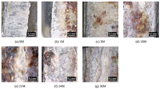
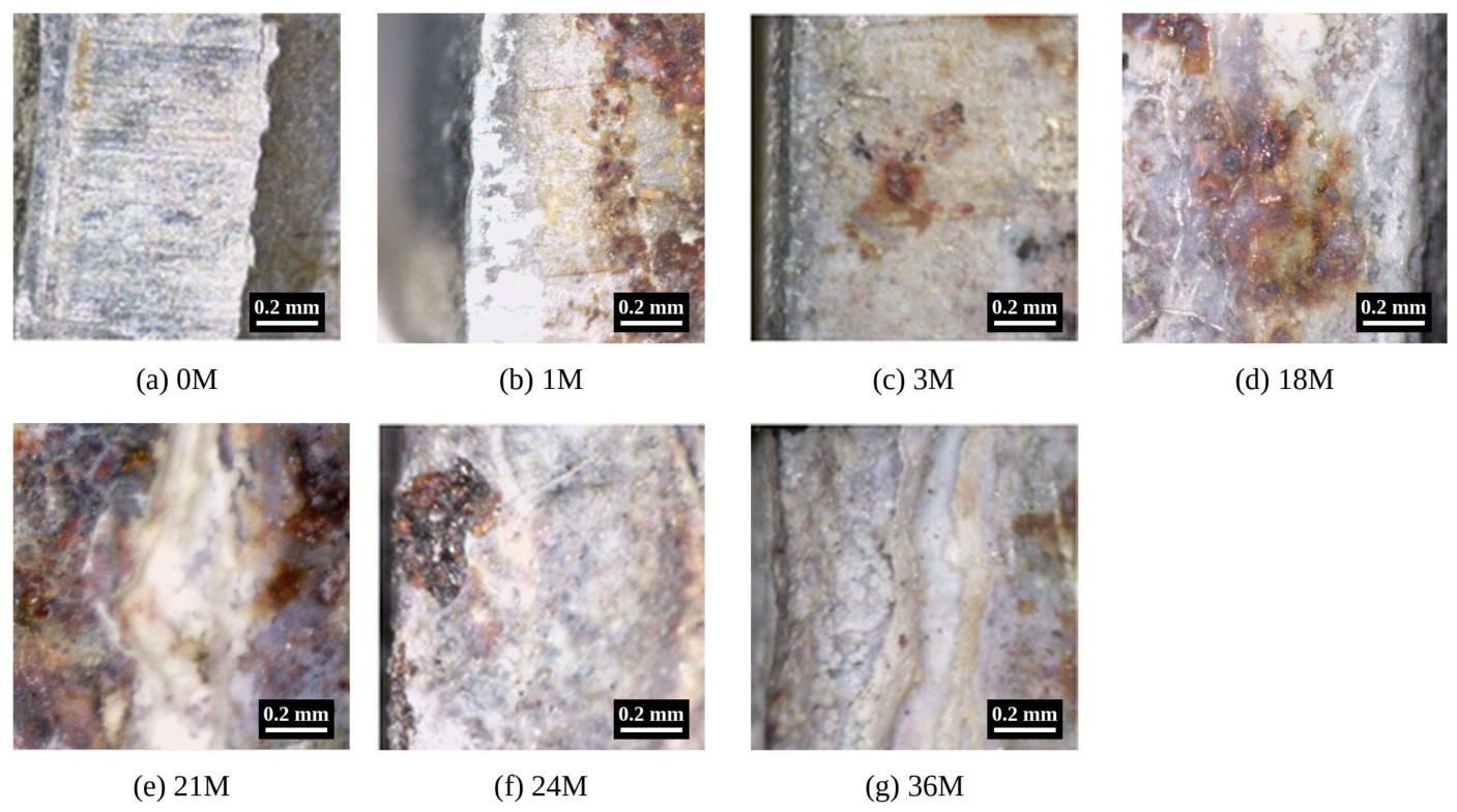
Optical image observation revealed progressive morphological changes with exposure time (Figure 1), consistent with image-based approaches previously used to characterize the progression of atmospheric corrosion [37]. At 0 months, the surface retained a relatively homogeneous metallic appearance with linear surface marks and negligible localized discoloration or aggregated reaction products. At 1 month, white to grey corrosion products covered part of the surface, and reddish-brown spots were present in the adjacent area. At 3 months, small brown spots were dispersed over a predominantly white surface.
Figure 1.
Representative optical micrographs of the specimen surface after (a) 0, (b) 1, (c) 3, (d) 18, (e) 21, (f) 24 and (g) 36 months of exposure. All images were taken with a digital optical microscope at 50× magnification. Brightness and contrast were not adjusted individually for each panel. The specimens were no longer available, so the images could not be re-acquired under uniform illumination. Scale bars: 0.2 mm.
A pronounced morphological change was observed at 18 months, where localized brown to yellowish-brown corrosion products appeared on a predominantly white/grey background, producing greater surface heterogeneity than at the earlier exposure periods. At 21 and 24 months, coarse reddish-brown and black products developed in concentrated local patches, indicative of intensified localized reactions. By 36 months, the prominence of reddish-brown and black products diminished and a grey-white coating layer became dominant again, suggesting further reorganization of the surface reaction at late exposure stages.
These morphological observations were broadly consistent with the EPMA-derived quantitative metrics. During 0–3 months, changes in median intensity and positive area ratio were limited. After 18 months, the spatial heterogeneity indicators (IQR, P95, hotspot area ratio and largest hotspot ratio) showed more pronounced variation. The coarse localized products at 21 and 24 months coincided with a moderate O positive area ratio (0.10–0.14). At 36 months, the O positive area ratio returned to a low level (0.015) although the surface remained covered by corrosion product layers.
Overall, the time series is better described as a staged progression than as a monotonic accumulation. It consists of an initial coverage stage, a transient O-rich state first detected at 18 months, localized coarse products at 21–24 months and renewed product-layer dominance at 36 months.
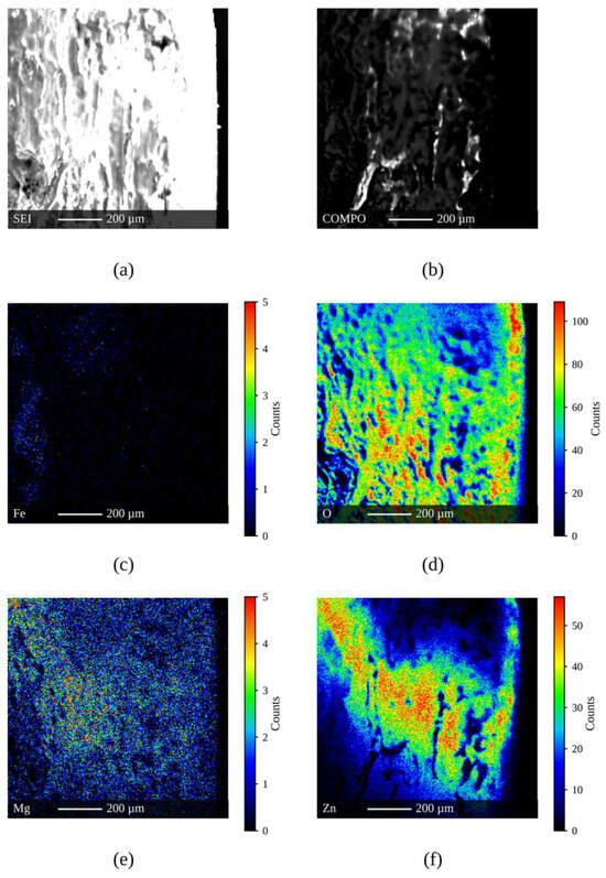
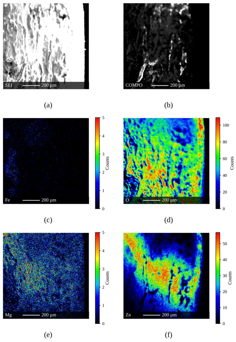
The 18-month EPMA elemental maps show the spatial distribution of this O-rich state (Figure 2). The O map exhibits a broadly distributed high-intensity signal across much of the analyzed surface, whereas the Fe signal remains sparse and localized. Zn is retained over a substantial portion of the mapped region but shows pronounced spatial heterogeneity. The Mg map is shown for reference. Mg is not a constituent of the HGI coating, and its signal may originate from airborne sea salt deposited at the coastal exposure site. Its origin could not be confirmed with the present data, so Mg was not included in the quantitative analysis. The spatial association between O and the other elements is summarized in Table S4. At 18 months, the O map was spatially continuous (Moran’s I = 0.90 ± 0.02). O correlated positively with Zn (ρ = 0.41 ± 0.23) but only weakly with Fe (ρ = 0.09 ± 0.08), and the O hotspots were slightly enriched in Zn-rich regions (enrichment factor 1.29). At the other exposure times, only 1–15% of the pixels showed a detectable O signal and the correlation coefficients were close to zero. These sparse maps do not allow the spatial association to be evaluated. The O-rich regions at 18 months therefore coincide with Zn-containing corrosion products rather than with Fe-rich areas. The extensive O-rich domains in Figure 2 are consistent with the high O positive area ratio quantified in the following sections.
Figure 2.
EPMA maps of the specimen surface after 18 months of exposure: (a) SEI, (b) COMPO, (c) Fe Lα, (d) O Kα, (e) Mg Kα and (f) Zn Kα. The color bars give the X-ray intensity in counts. The color scales run from 0 to the 99.5th percentile of each map, except for Fe, for which the full count range is shown. Scale bars: 200 µm.
3.2. Temporal Evolution of Median Elemental Intensities
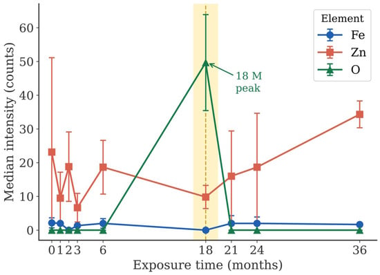
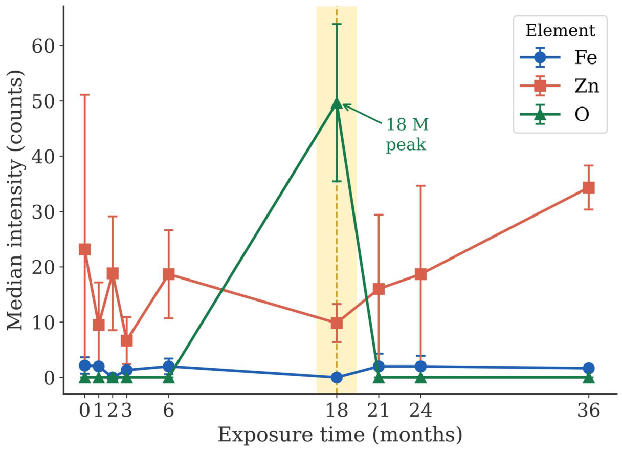
Figure 3 shows the temporal evolution of median elemental intensities for Fe, Zn, and O over 0–36 months. Fe medians remained low (0–2.2 counts) throughout the exposure. The low Fe value at 18 months is not compared with the other exposure times because Fe was recorded with the Lα line in this session (Table 1). Zn fluctuated during 0–6 months, with lower values at 1 and 3 months, and reached its highest value at 36 months. In contrast, O remained near zero at most time points but showed a marked spike exclusively at 18 months. The three elements therefore followed different temporal patterns.
Figure 3.
Temporal evolution of median elemental intensity (counts) for Fe, Zn and O over 0–36 months of exposure. Symbols show the mean of the six replicate maps and error bars show the standard deviation. The Fe value at 18 months was recorded with the Lα line. The yellow band and the dashed vertical line mark the 18-month exposure time.
3.3. Spatial Expansion of Oxygen Signal
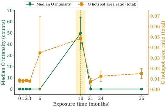
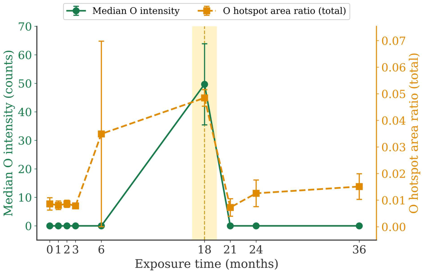
Figure 4 presents the co-evolution of O median intensity and O hotspot area ratio (total) over time. The hotspot area ratio exhibited a noticeable elevation and large inter-replicate variability at 6 months, suggesting the emergence of spatially heterogeneous O-rich regions during an intermediate stage. A more pronounced and concurrent response was observed at 18 months, when both the O median intensity and hotspot area ratio increased markedly. Thus, the 6-month behavior is interpreted as early localized heterogeneity, whereas the 18-month response reflects a broader reorganization of the oxygen-bearing surface products. At 21 months, both metrics declined.
Figure 4.
Co-evolution of O median intensity (counts; left axis) and O hotspot area ratio (total; right axis) over 0–36 months. Symbols show the mean of the six replicate maps and error bars show the standard deviation. The comparatively large variability at 6 months indicates pronounced inter-replicate spatial heterogeneity. The yellow band and the dashed vertical line mark the 18-month exposure time.
Within the sessions measured with the LDE1H crystal, the 18-month maps showed much higher O signals than the 21- and 24-month maps. The O median intensity was 51.5 counts at 18 months and 0 counts at 21 and 24 months, and the positive area ratio was 0.93 and 0.12, respectively (Mann–Whitney U test, p < 0.001). The O-rich state at 18 months therefore cannot be attributed to the change in the analyzing crystal.
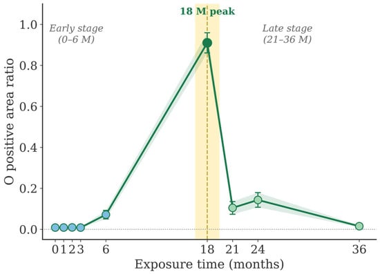
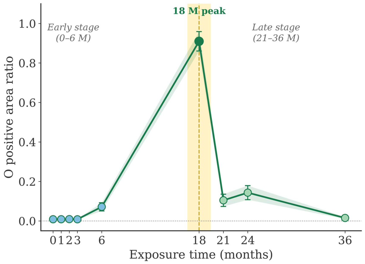
O positive area ratio (Figure 5) remained near zero during 0–3 months and increased modestly at 6 months before rising sharply to its maximum at 18 months (0.91). At this time point, a detectable O signal was present over most of the map area. The ratio declined at 21 months (0.10), increased slightly at 24 months (0.14) and returned to a low level at 36 months (0.015).
Figure 5.
Temporal evolution of O positive area ratio (fraction of map pixels with intensity > 0) over 0–36 months. Symbols show the mean of the six replicate maps and error bars show the standard deviation. The yellow band and the dashed vertical line mark the 18-month exposure time. Blue, dark green and light green symbols denote the early, 18-month and late exposure times, respectively. The green shading indicates the standard deviation.
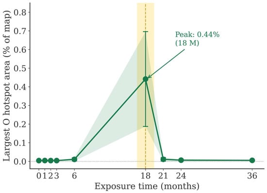
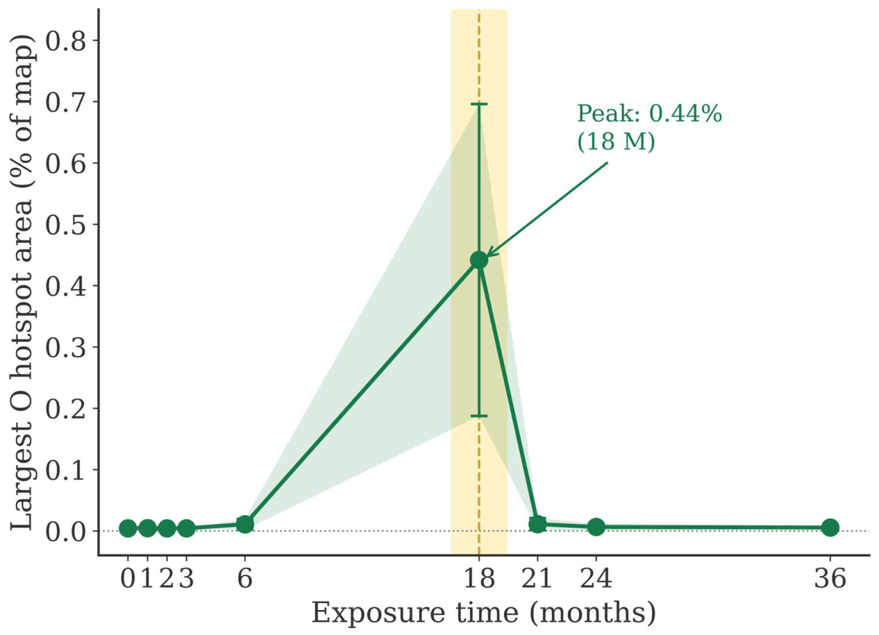
O largest hotspot ratio (total) (Figure 6) was negligible at early (0–3 months) and late (21–36 months) time points but peaked at 18 months. The largest connected O-rich hotspot occupied approximately 0.44% of the total mapped area at this time. Although this absolute area fraction was small, it represented a pronounced increase relative to the other exposure periods, indicating enhanced spatial connectivity of high-intensity O-rich regions rather than extensive macroscopic surface coverage.
Figure 6.
Temporal evolution of O largest hotspot ratio (total; largest connected hotspot component area normalized by total map area) over 0–36 months. Symbols show the mean of the six replicate maps and error bars show the standard deviation. The peak at 18 months corresponds to approximately 0.44% of the total mapped area. The yellow band and the dashed vertical line mark the 18-month exposure time. The green shading indicates the standard deviation.
3.4. Statistical Test Results
Kruskal–Wallis tests showed significant month-level differences after FDR correction for seven of the eight O-based features. These were the median, IQR, P95, positive area ratio, hotspot area ratio (total), hotspot area ratio (positive) and largest hotspot ratio (total) (Table S1). Only the hotspot component count was not significant. Seven of the eight Fe features also varied between months. Part of this variation arises from the 18-month session, in which Fe was recorded with the Lα line. Among the Zn features, only P95 and the largest hotspot ratio were significant.
Mann–Whitney U tests comparing the early (0–6 months) and late (18–36 months) periods showed significant differences after FDR correction for the same seven O-based features (Table S2). The effect sizes were largest for the positive area ratio (r = 0.828), followed by P95 (r = 0.625) and the largest hotspot ratio (r = 0.431). Only one Fe feature (largest hotspot ratio, r = −0.425) and one Zn feature (P95, r = 0.428) reached significance. The Fe and Zn features therefore did not show the consistent pattern observed for O. The extent of the O detection area was the most strongly differentiated characteristic between the two periods.
The largest hotspot ratio differed significantly between the two periods under all six threshold definitions (FDR-adjusted p ≤ 0.035; Table S5). The hotspot area ratio (total) was significant under five of the six definitions. The hotspot area ratio (positive) and the hotspot component count depended on the threshold definition and are therefore not interpreted further.
Dunn’s post-hoc test on O median intensity showed that the 18-month time point differed significantly from all other time points (0, 1, 2, 3, 6, 21, 24, and 36 months; adjusted p < 0.001; Table S3). The pairwise comparisons among the remaining time points were not significant. With respect to the O median, 18 months therefore behaved as a statistically distinct state rather than as a point within a gradual continuum.
3.5. Comparison of Temporal Models
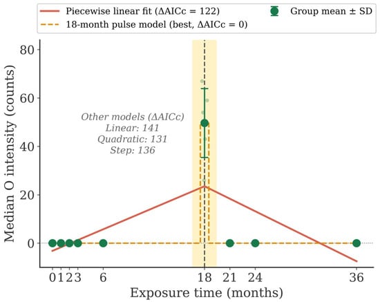
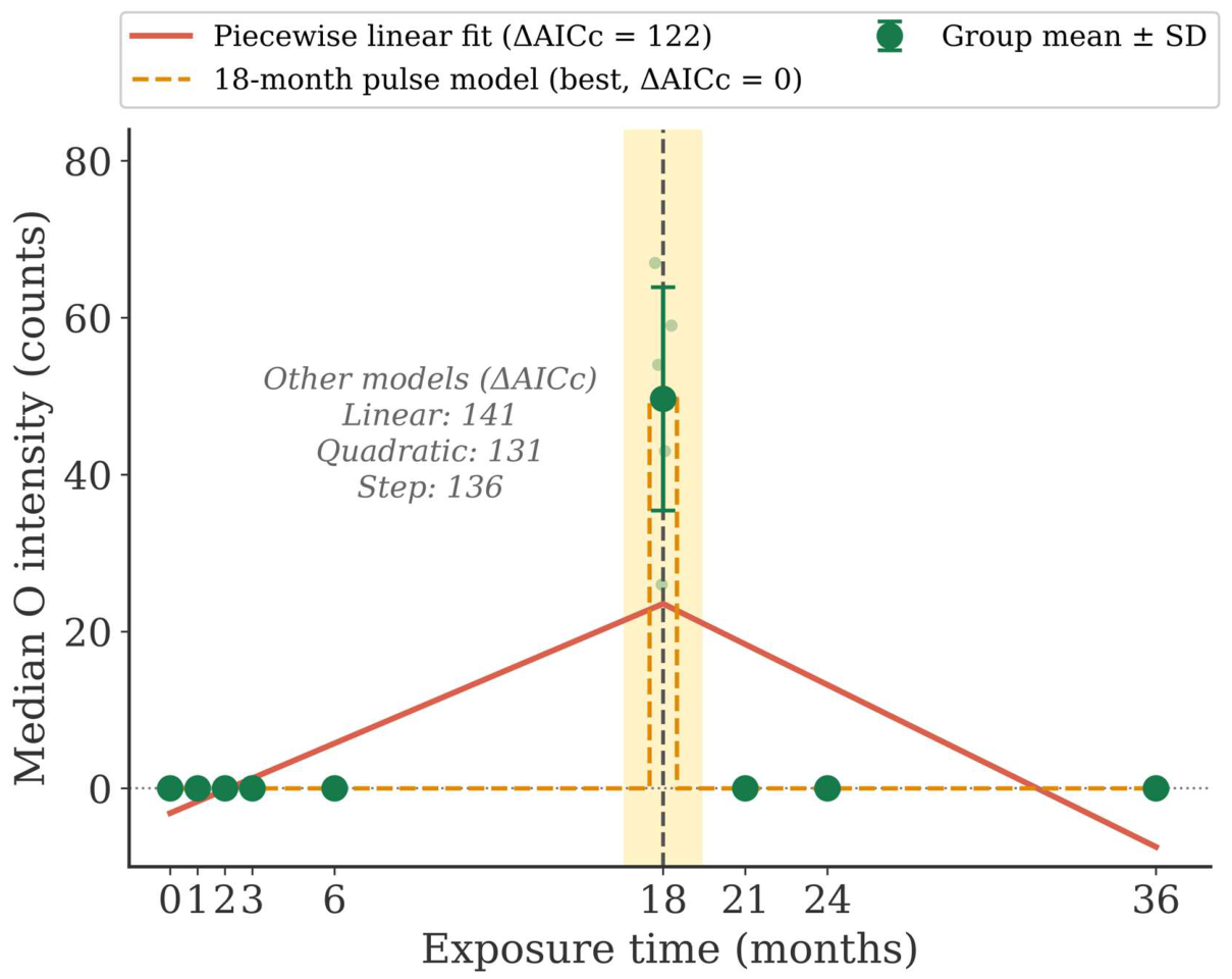
Figure 7 compares five temporal models fitted to the replicate-level O median intensity. The 18-month pulse model gave the lowest AICc, and all alternative models had ΔAICc > 120. The same ranking was obtained for the O positive area ratio and the largest hotspot ratio, for which all alternative models had ΔAICc > 60. The 18-month response is therefore not supported as a change in the slope of a continuous trend and is better described as a localized maximum.
Figure 7.
Comparison of temporal models fitted to the replicate-level O median intensity (n = 54). The 18-month pulse model and the piecewise linear fit are drawn, and the ΔAICc values of the linear, quadratic and step models are given in the panel. Light symbols show individual replicate maps and dark symbols show the group mean ± SD. ΔAICc is given relative to the best model. The yellow band and the dashed vertical line mark the 18-month exposure time. The horizontal dotted line marks zero intensity.
4. Discussion
The principal finding of this study is that the dominant temporal signature in the EPMA maps of HGI steel is not a gradual increase in elemental intensity but a change in the spatial distribution of oxygen-bearing corrosion products, which was most pronounced at 18 months. This conclusion does not rest on a single indicator. O-based features describing central tendency (median), distributional breadth (IQR), upper-tail intensity (P95), detection area (positive area ratio) and spatial connectivity (largest hotspot ratio) were significant after FDR correction in both the Kruskal–Wallis and Mann–Whitney U frameworks. The largest hotspot ratio also remained significant under all six hotspot threshold definitions. This multivariate consistency reduces the probability of a spurious finding. The tests are nevertheless exploratory because the replicate maps at each exposure time came from one specimen.
Dunn’s post-hoc test identified the 18-month O median as distinct from every other time point, whereas the comparisons among the other time points were not significant. The temporal model comparison gives the same picture. A pulse confined to 18 months described the O data far better than linear, quadratic, step and piecewise models, so the 18-month response is a localized maximum rather than a lasting change in slope. Within the sessions measured with the LDE1H crystal, the 18-month maps also showed a much higher O signal than the 21- and 24-month maps. The O-rich state is therefore not an artifact of the analyzing crystal. The effect size hierarchy (positive area ratio > P95 > largest hotspot ratio) indicates that the 18-month state is characterized mainly by an expansion of the O-detectable area. This expansion was accompanied by a stronger upper-tail signal and larger connected high-intensity regions.
The threshold sensitivity analysis showed that the hotspot component count and the hotspot area ratio (positive) depend on the threshold definition. Before 18 months, nearly all positive O pixels had a value of 1 count, so the relative thresholds collapsed to this value. These two features therefore cannot show whether the O-rich regions grew by the coalescence of existing sites or by the nucleation of new ones.
The EPMA maps show where oxygen-bearing products are located and how their distribution changed between the exposure times. They do not identify the phases, so the following interpretation is a hypothesis. The O-rich domains at 18 months coincided with Zn-rich regions and may consist of ZnO, Zn(OH)2 or zinc hydroxy salts formed by local redistribution of the earlier corrosion products [3,4,5,6,7,8,9,10,11]. The decline of the O metrics after 18 months may reflect partial dissolution or recrystallization of these products, or their coverage by a secondary Zn-rich layer, as the Zn median increased toward 36 months. These interpretations require confirmation using phase-sensitive methods such as XRD or Raman spectroscopy and by cross-sectional microstructural analysis [20].
In contrast to O, the Fe and Zn features did not show a consistent difference between the early and late periods. This does not imply that these elements are unimportant to the corrosion process. It indicates that the primary statistical signature of the change in the present data is carried by oxygen distribution. Fe and Zn changes may better represent consequences or antecedents of the oxygen reorganization than independent markers in this time series. The interpretation of Fe at 18 months is further limited because Fe was recorded with the Lα line in this session. Multi-element interaction analysis or path modeling may be warranted in future work.
Several limitations deserve consideration. First, only one specimen was analyzed at each exposure time. Because the six maps at each exposure time were obtained from a single specimen, variability between specimens could not be assessed. The statistical comparisons therefore describe differences between the analyzed specimens and should be regarded as exploratory. Second, the data show a transient O-rich state at 18 months. It was observed in all six maps and was not reproduced at 21 and 24 months under the same measurement conditions. Because only one specimen was analyzed at each exposure time and no specimens were examined between 6 and 18 months, it cannot be determined whether this state reflects a general stage of the corrosion process or a feature of the 18-month specimen.
Third, the pre/post 18-month comparison combines sessions measured with different O analyzing crystals. Its effect sizes for O are therefore partly influenced by the difference in detection efficiency, and they are interpreted together with the comparison within the LDE1H sessions. Fourth, the relative hotspot threshold describes the structure within each map and does not by itself allow absolute comparisons between maps. Absolute O intensities were therefore compared only between sessions measured with the same analyzing crystal. Fifth, the environmental parameters were recorded as daily or monthly values at the exposure site and not at the specimen surface. Time of wetness and gaseous pollutants such as SO2 and NO2 were not measured. The observed changes in the corrosion products could therefore not be linked to specific environmental events, and seasonal effects between the sampling times cannot be excluded. Finally, mechanistic confirmation requires spectroscopic and microstructural methods that directly identify the corrosion product phases.
5. Conclusions
Time-series EPMA elemental maps of HGI steel exposed outdoors for 0–36 months were analyzed using robust distributional features and spatial hotspot metrics to examine the change in the oxygen distribution observed at 18 months. The principal conclusions are:
(1) Several O-based indicators, including the median, IQR, P95, positive area ratio and largest hotspot ratio, differed significantly between the early (0–6 months) and late (18–36 months) periods after FDR correction. Fe and Zn features did not show a comparable consistent pattern.
(2) The largest effect size was observed for the O positive area ratio (rank-biserial r = 0.828), followed by P95 (r = 0.625) and the largest hotspot ratio (r = 0.431). The largest hotspot ratio remained significant under six hotspot threshold definitions. Spatial expansion of the detectable O signal was thus the dominant feature of the change.
(3) The hotspot component count depended on the threshold definition, so the mode of growth of the O-rich regions could not be determined.
(4) The 18-month O signal is best described as a transient maximum. It was not reproduced at 21 and 24 months under the same measurement conditions, and an 18-month pulse model described the O data better than linear, quadratic, step and piecewise models. At 18 months, the O signal was spatially continuous and coincided with Zn-rich regions.
(5) The proposed framework, which combines robust distributional features with connectivity-based spatial metrics, provides a quantitative approach for characterizing time-dependent changes in EPMA maps of coated steel surfaces. Its application to other zinc-based or multi-component coatings is possible in principle but remains to be validated.
Supplementary Materials
The following supporting information can be downloaded at: https://www.mdpi.com/article/10.3390/met16121282/s1, Table S1: Kruskal–Wallis tests across the nine exposure times (0, 1, 2, 3, 6, 18, 21, 24 and 36 months) for all elements and map features; Table S2: Mann–Whitney U tests comparing the exposure times before (< 18 months; 0, 1, 2, 3 and 6 months) and after (≥ 18 months; 18, 21, 24 and 36 months) 18 months; Table S3: Dunn’s post-hoc pairwise comparisons of O median intensity between exposure times; Table S4: Spatial association of the O maps with the Zn and Fe maps at each exposure time (mean ± standard deviation of the replicate maps). Table S5: Sensitivity of the O hotspot features to the threshold definition (Mann–Whitney U test before vs. after 18 months and Kruskal–Wallis test across all exposure times).
Author Contributions
Conceptualization, B.K.; methodology, M.L.; software, B.K. and J.K.; validation, B.K.; formal analysis, J.-H.Y.; investigation, S.W. and J.P.; resources, M.L. and J.-H.Y.; data curation, S.W. and J.P.; writing—original draft preparation, B.K.; writing—review and editing, J.Y.; visualization, J.K.; supervision, J.Y.; funding acquisition, J.Y. All authors have read and agreed to the published version of the manuscript.
Funding
This research was a part of the project titled ‘Training Blue Tech Leaders for Eco-Friendly Ships (No. RS-2025-02220459)’, funded by the Ministry of Oceans and Fisheries, Korea.
Data Availability Statement
The data presented in this study are available on request from the corresponding author. The data are not publicly available because the raw datasets are part of an ongoing follow-up study.
Conflicts of Interest
Author Ji-Hoon Yang was employed by the company POSCO. The remaining authors declare that the research was conducted in the absence of any commercial or financial relationships that could be construed as a potential conflict of interest.
Abbreviations
The following abbreviations are used in this manuscript:
| AICc | Small-sample corrected Akaike information criterion |
| COMPO | Backscattered electron composition image |
| EPMA | Electron probe microanalysis |
| FDR | False discovery rate |
| HGI | Hot-dip galvanized iron |
| IQR | Interquartile range |
| P95 | 95th percentile |
| SEI | Secondary electron image |
References
- Llovet, X.; Moy, A.; Pinard, P.T.; Fournelle, J.H. Reprint of: Electron probe microanalysis: A review of recent developments and applications in materials science and engineering. Prog. Mater. Sci. 2021, 120, 100818. [Google Scholar] [CrossRef] [Scilit]
- Goldstein, J.I.; Newbury, D.E.; Michael, J.R.; Ritchie, N.W.M.; Scott, J.H.J.; Joy, D.C. Scanning Electron Microscopy and X-Ray Microanalysis; Springer: New York, NY, USA, 2018. [Google Scholar] [CrossRef] [Scilit]
- Leygraf, C.; Odnevall Wallinder, I.; Tidblad, J.; Graedel, T. Atmospheric Corrosion, 2nd ed.; Wiley: Hoboken, NJ, USA, 2016. [Google Scholar] [CrossRef] [Scilit]
- Persson, D.; Thierry, D.; Karlsson, O. Corrosion and corrosion products of hot dipped galvanized steel during long term atmospheric exposure at different sites world-wide. Corros. Sci. 2017, 126, 152–165. [Google Scholar] [CrossRef] [Scilit]
- Cole, I.S. Recent progress and required developments in atmospheric corrosion of galvanised steel and zinc. Materials 2017, 10, 1288. [Google Scholar] [CrossRef] [Scilit] [PubMed]
- Wallinder, I.O.; Leygraf, C. A critical review on corrosion and runoff from zinc and zinc-based alloys in atmospheric environments. Corrosion 2017, 73, 1060–1077. [Google Scholar] [CrossRef] [Scilit] [PubMed]
- Chen, Y.Y.; Chung, S.C.; Shih, H.C. Studies on the initial stages of zinc atmospheric corrosion in the presence of chloride. Corros. Sci. 2006, 48, 3547–3564. [Google Scholar] [CrossRef] [Scilit]
- De la Fuente, D.; Castaño, J.G.; Morcillo, M. Long-term atmospheric corrosion of zinc. Corros. Sci. 2007, 49, 1420–1436. [Google Scholar] [CrossRef] [Scilit]
- Neufeld, A.K.; Cole, I.S.; Bond, A.; Furman, S.A. The initiation mechanism of corrosion of zinc by sodium chloride particle deposition. Corros. Sci. 2002, 44, 555–572. [Google Scholar] [CrossRef] [Scilit]
- Odnevall, I.; Leygraf, C. The formation of Zn4SO4(OH)6·4H2O in a rural atmosphere. Corros. Sci. 1994, 36, 1077–1087. [Google Scholar] [CrossRef] [Scilit]
- Veleva, L.; Acosta, M.; Meraz, E. Atmospheric corrosion of zinc induced by runoff. Corros. Sci. 2009, 51, 2055–2062. [Google Scholar] [CrossRef] [Scilit]
- de Azevedo Alvarenga, E.; de Freitas Cunha Lins, V. Atmospheric corrosion evaluation of electrogalvanized, hot-dip galvanized and galvannealed interstitial free steels using accelerated field and cyclic tests. Surf. Coat. Technol. 2016, 306, 428–438. [Google Scholar] [CrossRef] [Scilit]
- Graedel, T.E. Corrosion mechanisms for zinc exposed to the atmosphere. J. Electrochem. Soc. 1989, 136, 193C–203C. [Google Scholar] [CrossRef] [Scilit]
- Daniel, E.F.; Wang, C.; Li, C.; Dong, J.; Udoh, I.I.; Zhang, D.; Zhong, W.; Zhong, S. Evolution of corrosion degradation in galvanised steel bolts exposed to a tropical marine environment. J. Mater. Res. Technol. 2023, 27, 5177–5190. [Google Scholar] [CrossRef] [Scilit]
- Daniel, E.F.; Wang, C.; Li, C.; Dong, J.; Udoh, I.I.; Zhang, D.; Zhong, W.; Zhong, S. Atmospheric corrosion performance of structural steel bolts in the Wenchang marine environment, South China. Eng. Fail. Anal. 2023, 150, 107352. [Google Scholar] [CrossRef] [Scilit]
- Bunphot, A.; Sancharoen, P.; Tangtermsirikul, S.; Chaisomphob, T. Atmospheric corrosion of hot dip galvanized structural steel exposed to the tropical climate of Thailand. J. Met. Mater. Miner. 2025, 35, e2115. [Google Scholar] [CrossRef] [Scilit]
- Said Ahmed, M.; Lebrini, M. Electrochemical study of the influence of H2S on atmospheric corrosion of zinc in Sargassum-affected tropical environments. Metals 2026, 16, 31. [Google Scholar] [CrossRef] [Scilit]
- Diler, E.; Rouvellou, B.; Rioual, S.; Lescop, B.; Vien, G.N.; Thierry, D. Characterization of corrosion products of Zn and Zn-Al-Mg coated steel in a marine atmosphere. Corros. Sci. 2014, 87, 111–117. [Google Scholar] [CrossRef] [Scilit]
- Odnevall, I.; Leygraf, C. Reaction Sequences in Atmospheric Corrosion of Zinc. In Atmospheric Corrosion; ASTM STP 1239; Kirk, W.W., Lawson, H.H., Eds.; American Society for Testing and Materials: Philadelphia, PA, USA, 1995; pp. 215–229. [Google Scholar] [CrossRef] [Scilit]
- Liu, Y.; Ooi, A.; Tada, E.; Nishikata, A. Electrochemical monitoring of the degradation of galvanized steel in simulated marine atmosphere. Corros. Sci. 2019, 147, 273–282. [Google Scholar] [CrossRef] [Scilit]
- Qiao, C.; Shen, L.; Hao, L.; Mu, X.; Dong, J.; Ke, W.; Liu, J.; Liu, B. Corrosion kinetics and patina evolution of galvanized steel in a simulated coastal-industrial atmosphere. J. Mater. Sci. Technol. 2019, 35, 2345–2356. [Google Scholar] [CrossRef] [Scilit]
- Thierry, D.; Persson, D.; Luckeneder, G.; Stellnberger, K.-H. Atmospheric corrosion of ZnAlMg coated steel during long term atmospheric weathering at different worldwide exposure sites. Corros. Sci. 2019, 148, 338–354. [Google Scholar] [CrossRef] [Scilit]
- Esmaily, M.; Mortazavi, N.; Svensson, J.E.; Johansson, L.G. Evidence for an unusual temperature dependence of the atmospheric corrosion of zinc. J. Electrochem. Soc. 2016, 163, C864–C872. [Google Scholar] [CrossRef] [Scilit]
- Kang, C.; Kong, D.; Yao, J.; Guo, C.; Wang, L.; Xiao, K.; Dong, C.F. Long-term monitoring of zinc corrosion behavior in typical hot and dry atmosphere environment in Turpan, China. Anti-Corros. Methods Mater. 2018, 65, 471–483. [Google Scholar] [CrossRef] [Scilit]
- Donovan, J.J.; Allaz, J.M.; von der Handt, A.; Seward, G.G.E.; Neill, O.; Goemann, K.; Chouinard, J.; Carpenter, P.K. Quantitative WDS compositional mapping using the electron microprobe. Am. Mineral. 2021, 106, 1717–1735. [Google Scholar] [CrossRef] [Scilit]
- Marder, A.R. The metallurgy of zinc-coated steel. Prog. Mater. Sci. 2000, 45, 191–271. [Google Scholar] [CrossRef] [Scilit]
- Maurya, A.K.; Tiwari, S.; Bhavani, A.G.; Park, N.; Reddy, N.G.S. Artificial neural network-based modeling of atmospheric zinc corrosion rates using meteorological and pollutant data. Coatings 2025, 15, 538. [Google Scholar] [CrossRef] [Scilit]
- Gonzalez, R.C.; Woods, R.E. Digital Image Processing, 3rd ed.; Pearson Prentice Hall: Upper Saddle River, NJ, USA, 2008. [Google Scholar]
- Moran, P.A.P. Notes on continuous stochastic phenomena. Biometrika 1950, 37, 17–23. [Google Scholar] [CrossRef] [Scilit]
- Kruskal, W.H.; Wallis, W.A. Use of ranks in one-criterion variance analysis. J. Am. Stat. Assoc. 1952, 47, 583–621. [Google Scholar] [CrossRef]
- Mann, H.B.; Whitney, D.R. On a test of whether one of two random variables is stochastically larger than the other. Ann. Math. Stat. 1947, 18, 50–60. [Google Scholar] [CrossRef] [Scilit]
- Benjamini, Y.; Hochberg, Y. Controlling the false discovery rate: A practical and powerful approach to multiple testing. J. R. Stat. Soc. B 1995, 57, 289–300. [Google Scholar] [CrossRef] [Scilit]
- Dunn, O.J. Multiple comparisons using rank sums. Technometrics 1964, 6, 241–252. [Google Scholar] [CrossRef]
- Muggeo, V.M.R. Estimating regression models with unknown break-points. Stat. Med. 2003, 22, 3055–3071. [Google Scholar] [CrossRef] [Scilit] [PubMed]
- Burnham, K.P.; Anderson, D.R. Model Selection and Multimodel Inference: A Practical Information-Theoretic Approach, 2nd ed.; Springer: New York, NY, USA, 2002. [Google Scholar]
- Hurvich, C.M.; Tsai, C.-L. Regression and time series model selection in small samples. Biometrika 1989, 76, 297–307. [Google Scholar] [CrossRef]
- Wang, S.; Song, S. Image analysis of atmospheric corrosion exposure of zinc. Mater. Sci. Eng. A 2004, 385, 377–381. [Google Scholar] [CrossRef] [Scilit]

Disclaimer/Publisher’s Note: The statements, opinions and data contained in all publications are solely those of the individual author(s) and contributor(s) and not of MDPI and/or the editor(s). MDPI and/or the editor(s) disclaim responsibility for any injury to people or property resulting from any ideas, methods, instructions or products referred to in the content. |
© 2026 by the authors. Licensee MDPI, Basel, Switzerland. This article is an open access article distributed under the terms and conditions of the Creative Commons Attribution (CC BY) license.