


Abstract
The pantograph–catenary system is the critical pathway for energy collection for high-speed trains, and its interfacial state directly affects current-collection quality and operational safety. Due to the coupled effects of multiple factors, the friction coefficient at the interface exhibits significant nonlinearity, time variability, and stochastic fluctuations, posing substantial challenges for friction-behavior prediction. To improve the prediction accuracy and generalization capability of friction-coefficient models under complex current-carrying conditions, a CNN-LSTM model optimized by a physics-informed Sparrow Search Algorithm, namely PISSA-CNN-LSTM, is proposed in this study. Based on current-carrying friction tests, the effects of current, contact load, and sliding speed on the dynamic evolution of the friction coefficient are analyzed. The physics-based regularities associated with operating conditions are further incorporated into the SSA-based hyperparameter optimization process, enabling directed optimization under physical constraints. The results show that PISSA-CNN-LSTM outperforms CNN-LSTM and SSA-CNN-LSTM in prediction accuracy, convergence speed, and optimization efficiency. The test-set R2 reaches 0.9904, and the optimization time is reduced by 49.38% compared with SSA-CNN-LSTM. This work provides a more accurate, robust, and interpretable modeling approach for predicting pantograph–catenary interfacial friction behavior under complex current-carrying conditions.
1. Introduction
1.1. Background
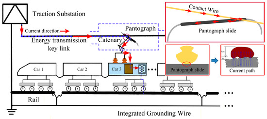
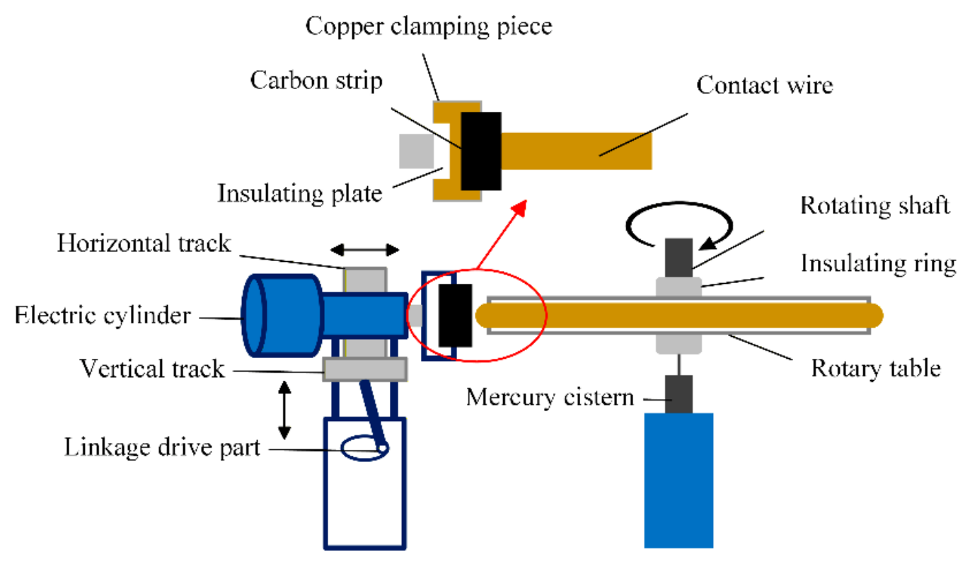
The pantograph carbon strip and copper contact wire of high-speed trains, hereafter referred to as the pantograph–catenary system, transfer electrical energy through sliding electrical contact and constitute the pathway through which the train receives electrical power [1,2] (Figure 1). Under the influence of operating conditions and environmental factors, wear of the C/Cu contact pair is inevitable during service. However, pantograph–catenary wear is not merely a process of mechanical material loss, but a complex interfacial evolution process involving electrical–thermal–mechanical multi-physics coupling [3,4]. With the advancement of the CR450 innovation project, further increases in train operating speed will intensify multi-physics coupling effects [5]. Abnormal wear and sustained arcing at the pantograph–catenary interface are therefore expected to occur more frequently [6], causing the evolution of the interfacial state to exhibit stronger nonlinearity, time variability, and stochasticity.
Figure 1.
Pantograph–catenary sliding electrical contact system.
To obtain comprehensive tribological data, a large number of repeated tests are usually required. However, tests under complex current-carrying operating conditions are often time-consuming and costly, with limited coverage of operating conditions, making it difficult to efficiently support rapid evaluation of interfacial behavior and prediction of interfacial states [7]. Therefore, establishing predictive models of pantograph–catenary friction behavior has become an important approach for improving evaluation efficiency. At present, most friction behavior models mainly focus on predicting the amount of wear on the strip. However, the wear amount generally reflects long-term damage accumulation at the pantograph–catenary interface and cannot readily characterize real-time changes in the interfacial contact state. In fact, the dynamic state of a current-carrying interface is multidimensional, encompassing both electrical-contact and tribological aspects. As a key parameter, dynamic contact resistance effectively reflects the electrical state of the interface, such as current-collection quality [8], and is therefore essential for evaluating electrical performance. Meanwhile, the dynamic friction coefficient serves as a highly sensitive indicator of the tribological state and can respond rapidly to material softening, damage, and other changes driven by multiphysics coupling. Because abnormal mechanical wear and dynamic instability directly compromise structural safety, this study specifically focuses on evaluating the tribological aspect. Therefore, dynamic prediction of the sliding friction coefficient of the pantograph–catenary system under complex current-carrying operating conditions is of significant engineering importance.
1.2. Literature Review
The dynamic evolution of the friction coefficient exhibits pronounced nonlinearity, temporal dependence, and multi-condition coupling characteristics. Traditional methods struggle to simultaneously perform local feature extraction and model long-term dynamic correlations. The CNN-LSTM model combines local feature extraction with long-term temporal dependency modeling and has been applied to complex friction-coefficient prediction. Song et al. fused multisource signals, including vibration and normal force, and used a CNN-LSTM–LightGBM hybrid model to diagnose wear states [9]. Under the optimal feature combination, the friction-coefficient prediction achieved an R2 greater than 0.971, demonstrating clear advantages in friction time-series modeling and nonlinear prediction. Yin et al. also used a CNN-LSTM model to predict the friction coefficients of various ceramic tribo-pairs under seawater lubrication conditions with different salinities and temperatures, achieving RMSE values below 0.001 [10]. These results further verify the high accuracy and applicability of the model for complex nonlinear friction time-series prediction. However, the model is highly sensitive to hyperparameters such as the number of convolutional kernels and the number of LSTM hidden-layer nodes, and manual hyperparameter tuning makes it difficult to obtain an optimal parameter combination that balances accuracy and generalization capability.
To improve optimization efficiency, researchers have introduced swarm intelligence optimization algorithms for automatic hyperparameter search. SSA has strong global search capability and rapid convergence, enabling automatic optimization of key parameters such as the learning rate and the number of network layers [11,12]. Wu et al. developed an SSA-XGBoost model to predict the friction coefficient of wet friction elements, achieving an RMSE of only 0.063, with 88.3% of predictions having relative errors below 1% [13]. Xia et al. used SSA-LSSVM to predict the friction coefficient of PTFE grease, increasing R2 by 8.91% and reducing RMSE by 52.05% [14]. These studies indicate that SSA is suitable for hyperparameter optimization in tribological prediction models.
However, the above models still follow a purely data-driven paradigm and strongly depend on the quality and quantity of training data. To improve the accuracy and generalization capability of complex friction and wear modeling, researchers have begun to integrate physical priors with data-driven models. Zhu et al. embedded wear evolution mechanisms into the prediction process, reducing RMSE by approximately 78.8% compared with traditional neural networks [15]. Kovalev et al. incorporated physical constraints such as friction-force decomposition relationships and contact load, enabling joint prediction of friction and wear behavior and contact state under limited data [16]. Pashmforoush et al. integrated a thermo-mechanical wear mechanism model, improving turning force prediction accuracy by 13–25% [17]. Zeng et al. integrated wheel–rail contact theory with the Archard model, reducing the composite metric by more than 42% [18]. These studies show that embedding physical priors into data-driven models can effectively improve prediction accuracy, physical consistency, and generalization capability.
Therefore, this study proposes a physics-informed PISSA-CNN-LSTM model for complex current-carrying friction conditions in the pantograph–catenary system, aiming to achieve highly accurate prediction of the dynamic interfacial friction coefficient.
1.3. Organization and Contributions
Section 2 investigates the effects of current, contact load, and sliding speed on the evolution of the dynamic friction coefficient at the pantograph–catenary interface using a ring-on-block current-carrying friction test platform. Section 3 develops a CNN-LSTM prediction framework that integrates operating-condition parameters with time-series features of the friction coefficient. On this basis, physics-based regularities associated with operating conditions are incorporated into the SSA-based hyperparameter optimization process. By dynamically reconstructing the search boundaries, the PISSA-CNN-LSTM model is established, thereby enabling model optimization under physical constraints.
The main contributions are as follows:
- The prediction target for the current-carrying friction interface of the pantograph–catenary system is extended from the conventional wear amount to the dynamic friction coefficient, thereby enhancing the sensitivity of real-time monitoring of the pantograph–catenary interfacial state.
- A physics-informed PISSA-CNN-LSTM model is proposed, in which operating-condition information is embedded into the search-space construction process, achieving simultaneous improvements in prediction accuracy, optimization efficiency, and physical consistency.
2. Current-Carrying Friction Test and Data Preprocessing
2.1. Test Platform
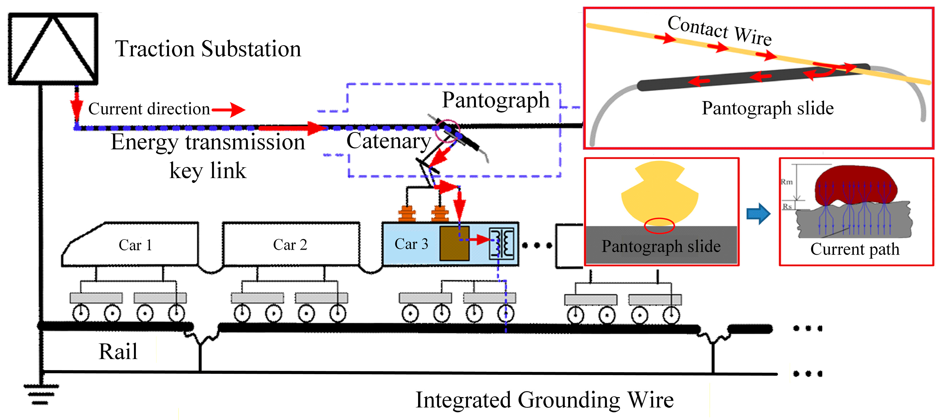
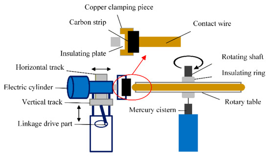
To investigate the friction and wear behavior of the C/Cu contact pair in the pantograph–catenary system under current-carrying conditions, experiments were conducted using a ring-on-block current-carrying friction simulation platform for pantograph–catenary contact (Figure 2). The platform mainly consists of a variable-speed motor, a rotating disk, a carbon slider clamping device, a connecting-rod driving mechanism, an electric cylinder, a DC power supply, and a control console. During the test, the copper contact wire was embedded along the outer circumference of the rotating disk, while the carbon slider was fixed in the clamping device. The variable-speed motor drove the rotating disk to simulate relative sliding between the pantograph–catenary contact pair. The connecting-rod driving mechanism was used to reproduce the zigzag relative motion between the carbon strip and the contact wire in an actual pantograph–catenary system. Direct current (DC) was applied to the C/Cu contact pair throughout the current-carrying friction tests. The platform allows continuous adjustment of the contact load, sliding speed, and DC within ranges of 10–300 N, 20–400 km/h, and 0–300 A, respectively. The interfacial voltage, current, normal force, and tangential friction force were measured synchronously using sensors and recorded at a sampling rate of 5 kHz for subsequent calculation of the friction coefficient.
Figure 2.
Current-carrying friction test platform.
The contact wire and strip materials used in the tests were obtained from an actual high-speed train pantograph–catenary system. The contact wire was made of pure copper, and the strip was made of pure carbon. The Key material properties of the contact wire and carbon strip are listed in Table 1. Before testing, the surface of the carbon strip was uniformly polished with 50#, 300#, and 2000# abrasive paper and run-in for 5 min under low-speed and no-current conditions to ensure a consistent initial contact state. The test conditions are listed in Table 2. Current, contact load, and sliding speed were selected as the three experimental variables, and 100 different parameter combinations were tested. Each operating condition was repeated three times to reduce the influence of random fluctuations on the results.
Table 1.
Key material properties of the contact wire and carbon strip.
Table 2.
Test conditions.
2.2. Data Processing
The friction coefficient is a key characteristic parameter for evaluating the tribological performance of the C/Cu contact pair in the pantograph–catenary system. Based on the synchronously measured dynamic friction force and dynamic normal force , the instantaneous friction coefficient at each sampling point was calculated using Equation (1), and the average friction coefficient over the statistical period was then obtained [19]:
where denotes the dynamic friction force at the i-th sampling point; denotes the dynamic normal force at the i-th sampling point; n is the number of valid sampling points; and denotes the average friction coefficient.
2.3. Dynamic Friction Coefficient Analysis
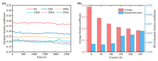
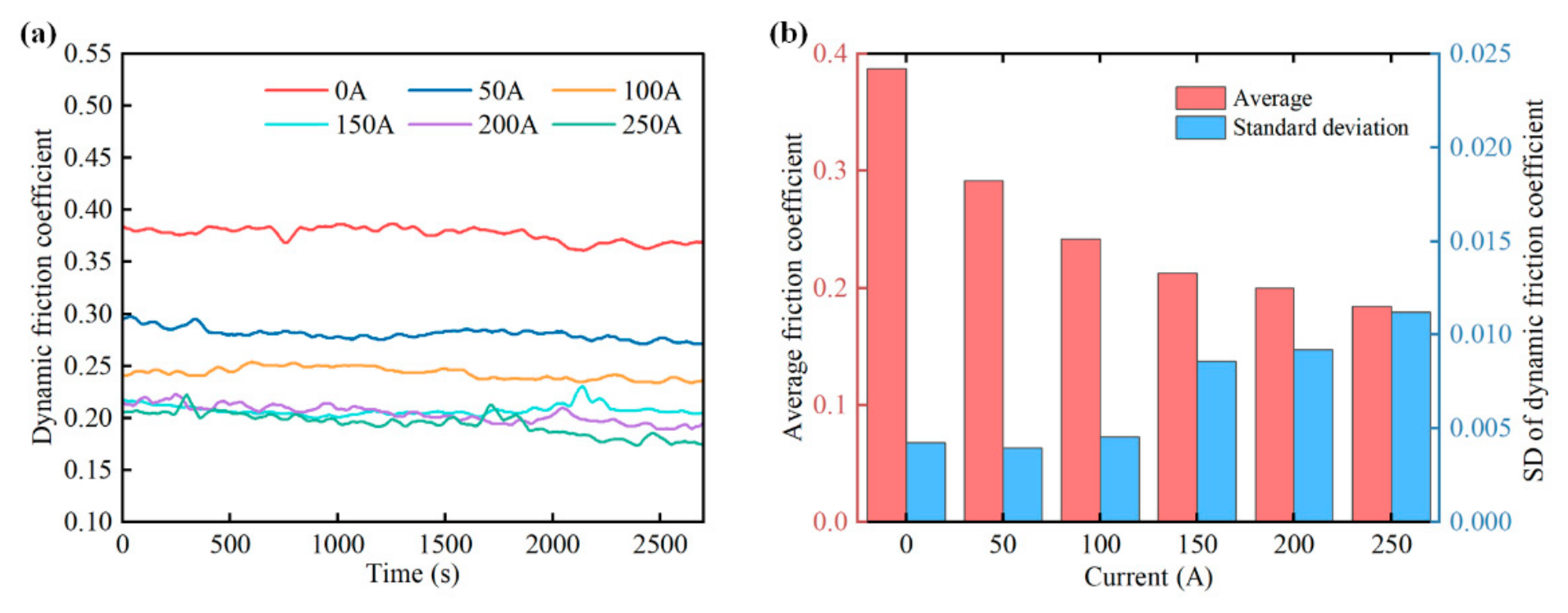
Under a contact load of F = 100 N and a sliding speed of v = 120 km/h, the temporal variations in the dynamic friction coefficient of the pantograph–catenary interface under different currents are shown in Figure 3a. In the absence of current, the dynamic friction coefficient is the highest and exhibits relatively small fluctuations. When the current increases to 150 A or above, the friction coefficient decreases significantly and stabilizes at approximately 0.18–0.20 in the later stage of the test, whereas its fluctuation amplitude increases markedly. As shown in Figure 3b, the average friction coefficient decreases monotonically with increasing current, while the standard deviation generally shows an increasing trend. This trend is mainly attributed to the increase in current, which intensifies the contact flash temperature and promotes thermal softening and plastic deformation of the copper asperities. These effects reduce their local shear strength and weaken the shearing and micro-cutting actions of the copper asperities on the carbon strip [20]. As the current continues to increase, the formation, deformation, and fracture of current-carrying contact asperities become more intense, while the arcing frequency and arc energy increase significantly [21], thereby intensifying friction-coefficient fluctuations.
Figure 3.
Friction characteristics under different currents: (a) dynamic friction coefficient; (b) average friction coefficient and standard deviation of dynamic friction coefficient.
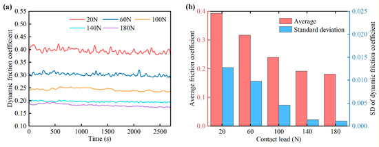
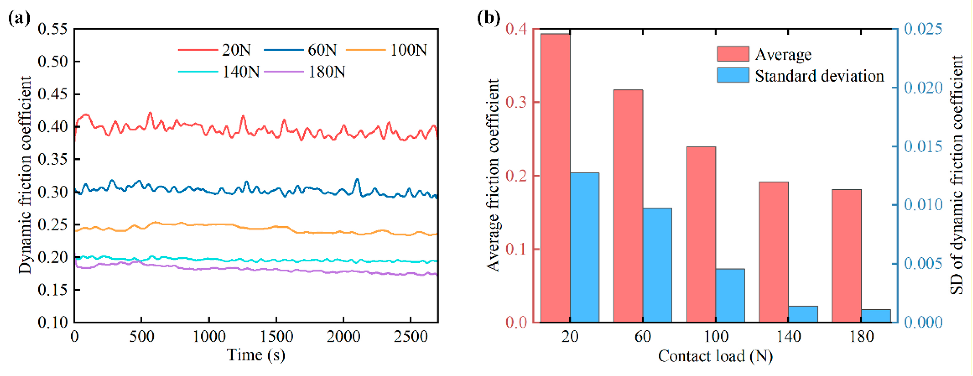
Under a current of I = 100 A and a sliding speed of v = 120 km/h, Figure 4a shows that the dynamic friction coefficient of the pantograph–catenary interface decreases with increasing contact load, while the fluctuation amplitude is significantly reduced. As shown in Figure 4b, the average friction coefficient continues to decrease as the load increases, and the standard deviation generally exhibits a downward trend. This indicates that increasing the contact load not only reduces the friction level of the pantograph–catenary interface but also suppresses friction fluctuations and improves operating stability. This can be mainly explained as follows. On the one hand, a higher load improves the mechanical contact stability of the interface and reduces the loss-of-contact rate of the pantograph–catenary system, thereby suppressing interfacial arcing and reducing friction-coefficient fluctuations [22,23,24]. On the other hand, the increased load promotes plastic deformation of interfacial asperities, reduces surface roughness, weakens the mechanical plowing effect [25], and facilitates the exfoliation and transfer of graphite, which is beneficial to the formation of lubricating graphite particles [26]. These effects jointly contribute to the reduction in the friction coefficient.
Figure 4.
Friction characteristics under different contact loads: (a) dynamic friction coefficient; (b) average friction coefficient and standard deviation of dynamic friction coefficient.
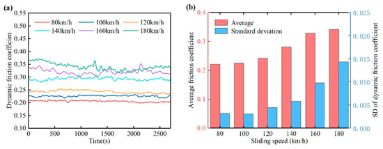
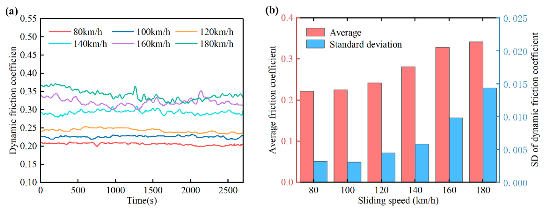
Under a current of I = 100 A and a contact load of F = 100 N, Figure 5a shows that the friction coefficient of the pantograph–catenary interface generally increases with increasing sliding speed, accompanied by a significant enhancement in fluctuation intensity. As shown in Figure 5b, both the average value and standard deviation of the friction coefficient increase with increasing sliding speed. This result indicates that a higher sliding speed increases the interfacial friction level and intensifies fluctuations in the friction process, thereby reducing operating stability. The main reason is that an increase in sliding speed strengthens the mechanical frictional interaction at the contact interface, leading to more severe mechanical wear [27]. Under the influence of arc ablation, metallic hard spots or localized surface irregularities may form on the contact wire surface. During high-speed operation, these defects are more likely to induce interfacial vibration and impact [28], resulting in unstable pantograph–catenary contact and even causing cracking and block detachment of the strip [29]. This further deteriorates the contact quality and wear characteristics [30], ultimately leading to an increased friction coefficient and intensified fluctuations.
Figure 5.
Friction characteristics at different sliding speeds: (a) dynamic friction coefficient; (b) average friction coefficient and standard deviation of dynamic friction coefficient.
3. PISSA-CNN-LSTM Model Construction
3.1. Construction of the CNN-LSTM Model
During actual service, the time-series signal of the friction coefficient of the pantograph strip contains both local transient characteristics and long-term evolutionary patterns. Therefore, a CNN-LSTM hybrid prediction model is constructed in this study. In this model, the CNN module employs one-dimensional convolutional layers to extract local fluctuation features induced by arcing disturbances, contact impacts, and abrupt changes in the contact interface state. Pooling layers are then used to reduce redundant information and improve the stability of feature representations. The extracted feature sequence is subsequently fed into the LSTM layer to model long-term dependencies, and the final prediction is generated through a fully connected layer.
3.2. SSA-Based Hyperparameter Optimization of the CNN-LSTM Model
The predictive performance of the CNN-LSTM model is strongly influenced by key hyperparameters, including the number of layers in the LSTM module, the number of hidden units, the batch size, the initial learning rate, and the L2 regularization coefficient. Relying on manual experience to determine these hyperparameters is not only highly subjective and inefficient but also makes it difficult to ensure that the model maintains strong adaptability under different operating conditions. To address this issue, the Sparrow Search Algorithm (SSA) is introduced in this study to adaptively optimize the key hyperparameters of the CNN-LSTM model.
SSA is a swarm intelligence optimization algorithm inspired by the foraging and anti-predator behaviors of sparrows [12]. In this algorithm, the population is divided into three types of individuals: producers, scroungers, and scouts. Producers are responsible for global exploration and guide the search direction of the population; scroungers perform local exploitation by following producers to improve search accuracy; and scouts maintain population diversity through positional perturbations, thereby reducing the risk of the algorithm becoming trapped in a local optimum. Through the coordinated updating of these three types of individuals, SSA can maintain a balance between global exploration and local exploitation, and offers advantages such as fast convergence, high optimization precision, and simple parameter configuration.
In the SSA-CNN-LSTM framework, the hyperparameter vector consisting of the number of LSTM layers, the number of hidden units, the batch size, the initial learning rate, and the L2 regularization coefficient is defined as the optimization variable. The root mean square error (RMSE) of the model predictions is used as the fitness function, with the objective of minimizing the RMSE. SSA searches for and optimizes candidate hyperparameter combinations through iterative population updates. The position update rules for producers, scroungers, and scouts are given in Equations (2)–(4), respectively:
where denotes the position of the i-th sparrow in the j-th dimension at iteration t; . denotes the maximum number of iterations; α is a random number in the interval (0, 1]; R2 and ST denote the warning value and the safety threshold, respectively; Q is a random number following a standard normal distribution; L is a vector of ones; d denotes the dimensionality of the search space; and denote the current global worst and best positions, respectively; denotes the best position of the current producer; is a random vector whose elements are randomly assigned values of +1 or −1; is the step-size control parameter; K is a random number in the interval [−1, 1]; , , and denote the fitness value of the current individual, the global best fitness value, and the worst fitness value, respectively; and ε is a small positive constant introduced to prevent division by zero.
Using the above iterative mechanism, SSA can identify hyperparameter combinations associated with lower prediction errors within a predefined search space, thereby reducing the burden of manual hyperparameter tuning and improving the model’s prediction accuracy and training stability. However, during hyperparameter optimization, standard SSA is essentially a “black-box” optimization method. Its search boundaries are primarily determined based on empirical experience, and the optimization process mainly depends on feedback from the fitness function. As a result, the physical information associated with the current-carrying friction process at the pantograph–catenary interface is not fully utilized, which may lead to ineffective searches and limited adaptability to varying operating conditions. Therefore, this study further incorporates physics-informed constraints to develop a PISSA optimization strategy.
3.3. Physics-Informed Search Space Reconstruction
To overcome the limitations of blind search in standard SSA, this study incorporates operating-condition information from the pantograph–sliding strip friction system into the construction of the SSA search space. Specifically, constraint relationships are established between the operating variables, including current, contact load, and sliding speed, and the hyperparameter search boundaries of the CNN-LSTM model. This enables a transition from a purely data-driven search strategy to a physics-informed and data-driven search strategy.
Let the operating-condition parameter set be denoted as , and link it to the hyperparameter vector of the CNN-LSTM model, , Here, , , , and correspond to the number of LSTM layers, the number of hidden units, the batch size, the initial learning rate, and the L2 regularization coefficient, respectively. The number of hidden units is mainly used to regulate the model’s representational capacity for complex time-series patterns, whereas the initial learning rate, L2 regularization coefficient, and batch size constrain the model training process in terms of training stability, generalization capability, and the smoothness of gradient estimates, respectively.
- (1)
- Influence of the current parameter. As the current approaches the high-current discharge regime, interface arcing and arc ablation become more pronounced, leading to stronger fluctuations in the time-series signal of the friction coefficient. Meanwhile, abrupt local variations and random disturbances become more frequent, resulting in increased signal complexity. Therefore, the upper search bound for the number of hidden units can be appropriately increased to enhance the model’s representational capacity for complex time-series patterns. In addition, under high-current conditions, parameter updates during training are more prone to oscillations. Accordingly, the upper search bound for the initial learning rate should be appropriately reduced as the current value increases, thereby improving training stability.
- (2)
- Influence of the contact load parameter. Under low-load conditions, contact stability at the interface is relatively poor, making contact loss and arcing more likely to occur. As a result, fluctuations and randomness in the time-series signal of the friction coefficient become more pronounced. Therefore, the upper search bound for the number of hidden units can be appropriately increased. Under high-load conditions, the interfacial contact gradually becomes more stable, and the time-series signal tends to stabilize. If excessively high model complexity is maintained, the model may overfit incidental fluctuations and secondary disturbances. Therefore, the L2 regularization constraint should be appropriately strengthened, and the model capacity should be properly reduced.
- (3)
- Influence of the sliding speed parameter. Under high-speed operating conditions, vibration-induced impacts at the interface and arcing become more pronounced, while the fluctuation amplitude and nonlinear complexity of the time-series signal of the friction coefficient increase simultaneously. Therefore, the upper search bound for the number of hidden units should also be appropriately increased. Meanwhile, because mini-batch training is more susceptible to increased variance in gradient estimates, the upper search bound for the batch size should be appropriately enlarged to reduce gradient-estimation variance and improve parameter-update stability. In addition, the number of LSTM layers is affected by the coupled effects of current, contact load, and sliding speed. Since the required depth of time-series modeling varies under different operating conditions, its search boundaries should be adjusted in a unified manner.
Based on the influence of the above operating-condition parameters on the search boundaries of different hyperparameters, the corresponding boundary adjustment coefficients are defined as follows: the coefficients describing the effects of current on the number of hidden units and the initial learning rate are denoted as and , respectively; the coefficients describing the effects of contact load on the number of hidden units and the L2 regularization coefficient are denoted as and , respectively; the coefficients describing the effects of sliding speed on the batch size and the number of hidden units are denoted as and , respectively; and the coefficient describing the coupled effect of multiple operating conditions on the number of LSTM layers is denoted as .
Based on the above adjustment coefficients, the search upper bounds of the hyperparameters are dynamically reconstructed. Let denote the original empirically defined upper bound and denote the dynamic upper bound obtained after applying physics-informed constraints. The search upper bounds for the number of LSTM layers, the number of hidden units, the batch size, the learning rate, and the L2 regularization coefficient can then be expressed as follows:
These expressions indicate that the adjustment coefficients are not directly involved in the forward calculation of the model output. Instead, they embed operating-condition information into the hyperparameter optimization process by reconstructing the search boundaries of the hyperparameters. Considering that the reconstructed boundaries may lead to an excessively narrow search interval or even coincident upper and lower bounds, a boundary correction operator is further introduced:
where LB denotes the search lower bound, denotes the absolute upper bound determined by hardware resource constraints, and is a small positive constant used to prevent the upper and lower bounds from coinciding. Based on the above operating-condition constraint relationships, search-boundary reconstruction, and boundary correction process, the hyperparameter optimization problem under physics-informed constraints is formulated as follows:
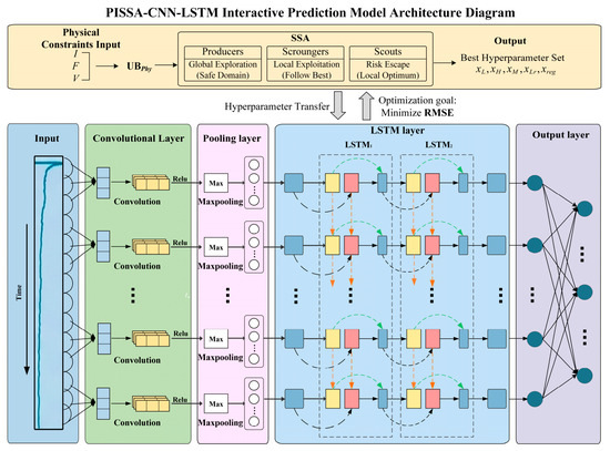
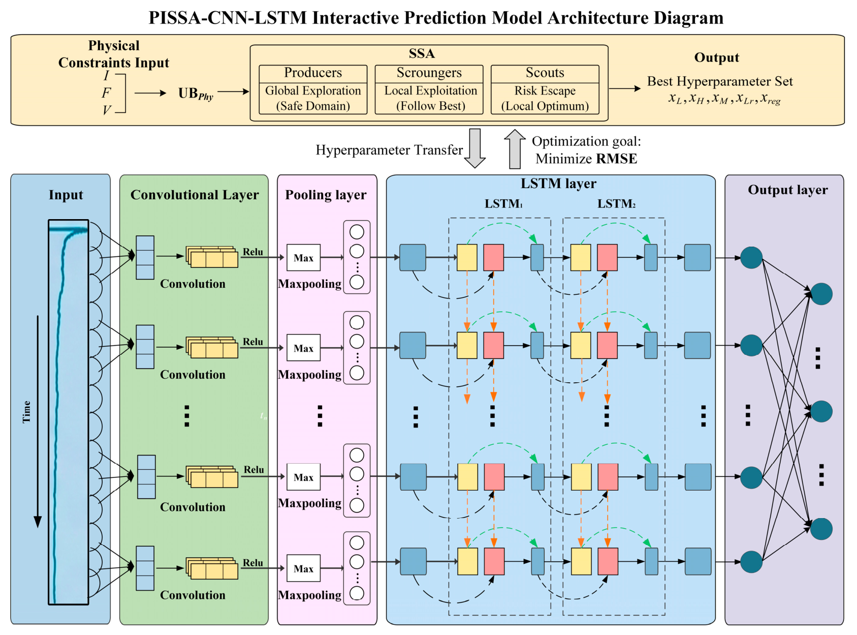
where denotes the optimal hyperparameter vector, denotes the feasible search domain after incorporating physics-informed constraints, denotes the loss function defined on the training set, and denote the training data and test data, respectively. This formulation indicates that, when SSA is used for hyperparameter optimization, the search is not conducted randomly within a unified fixed range. Instead, it is guided by physics-informed operating-condition constraints, thereby enabling a transition from a purely data-driven search strategy to a physics-informed and data-driven search strategy. Figure 6 presents the architecture of the PISSA-CNN-LSTM prediction model, which integrates the physics-informed search space reconstruction with the SSA optimization process.
Figure 6.
Architecture of the PISSA-CNN-LSTM prediction model.
4. Results and Discussion
To verify the effectiveness of the physics-informed Sparrow Search Algorithm (PISSA) in the hyperparameter optimization of the CNN-LSTM model, a current-carrying test condition was selected with a current of 150 A, a contact load of 120 N, and a sliding speed of 140 km/h. Data were collected for 45 min. After downsampling and normalization, the dataset was split into training and test sets at an 8:2 ratio in chronological order. The model outputs were denormalized and then compared with the measured values. The coefficient of determination (R2), root mean square error (RMSE), mean absolute error (MAE), and mean absolute percentage error (MAPE) were used as performance evaluation metrics.
Meanwhile, the RMSE calculated from the model predictions was used as the fitness function during the SSA-based hyperparameter optimization stage, with the objective of minimizing RMSE. The population size was set to 15, and the maximum number of iterations was set to 50. The CNN-LSTM model was trained using the Adam optimizer, with the maximum number of training epochs set to 50. All experiments were conducted on a computer equipped with an Intel i9-13900KS processor and 64 GB of 6400 MHz RAM. The programming environment was MATLAB R2021b.
4.1. Comparison and Analysis of Model Predictive Performance
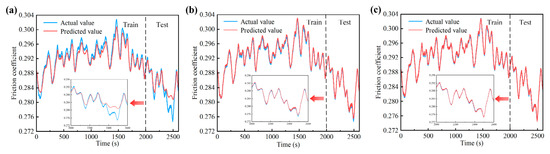
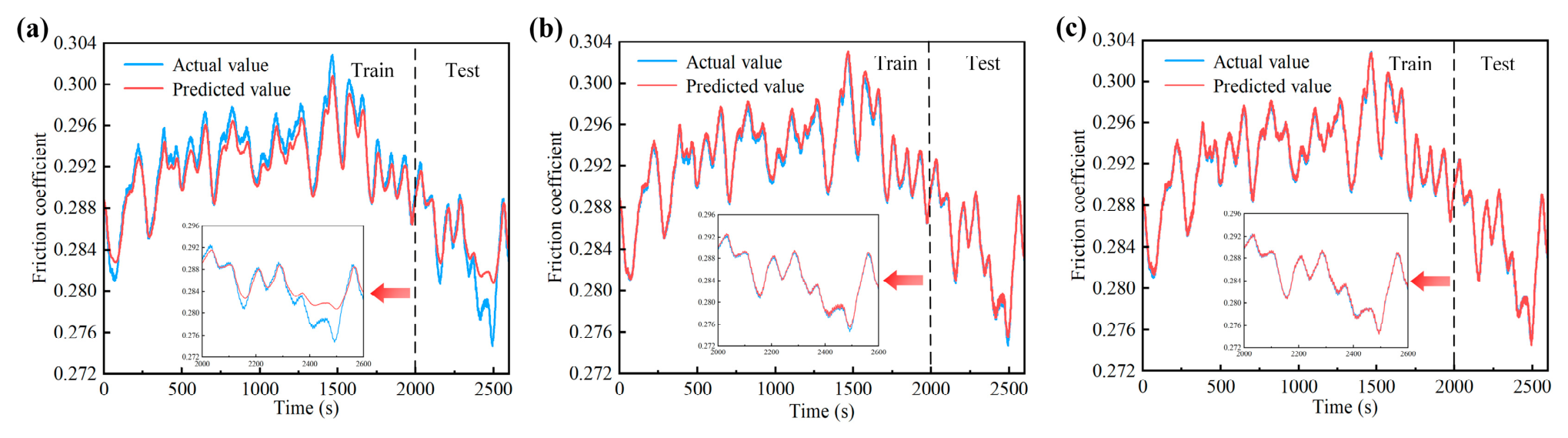
For the baseline CNN-LSTM model, the R2 value is 0.6753, while the RMSE and MAE are 2.1203 × 10⁻³ and 1.5837 × 10⁻³, respectively, and the MAPE is 0.3232%. As shown in Figure 7a, the predicted values in the test segment deviate markedly from the measured values in regions where the friction coefficient declines rapidly and exhibits sharp fluctuations, indicating that the CNN-LSTM model has difficulty effectively capturing complex abrupt features in the time-series signal.
Figure 7.
Comparison of friction coefficient prediction results obtained by different models: (a) CNN-LSTM, (b) SSA-CNN-LSTM, and (c) PISSA-CNN-LSTM.
After introducing SSA for hyperparameter optimization, the R2 value increases from 0.6753 to 0.9899, representing an improvement of 46.6%. Meanwhile, the RMSE decreases by approximately 82.4%, the MAE also decreases by 80.8%, and the MAPE drops from 0.3232% to 0.0618%, corresponding to an error reduction of more than fivefold. The prediction curve in Figure 7b shows a high degree of agreement with the measured values overall, indicating that the incorporation of SSA enhances the model’s fitting capability and predictive accuracy for the dynamic evolution of the friction coefficient.
PISSA provides a further, though modest, improvement over SSA in the overall performance metrics, with the R2 value increasing from 0.9899 to 0.9904, the RMSE decreasing by 2.4%, and the MAPE decreasing from 0.0618% to 0.0609%. It should be noted that the key advantage of PISSA does not lie in a substantial improvement in overall metrics, but rather in its ability to enhance the predictive stability and robustness of the model under complex operating conditions. The detailed performance metrics are presented in Table 3. A comparison of the zoomed-in views in Figure 7b,c shows that the SSA-CNN-LSTM model exhibits slight lag and oscillatory deviations in regions where the friction coefficient fluctuates sharply, whereas the prediction curve of the PISSA-CNN-LSTM model more closely matches the measured values. This indicates that it is better suited for predicting the behavior of highly dynamic current-carrying friction interfaces.
Table 3.
Performance evaluation metrics of the three models on the test set.
4.2. Hyperparameter Optimization and Convergence Efficiency Analysis
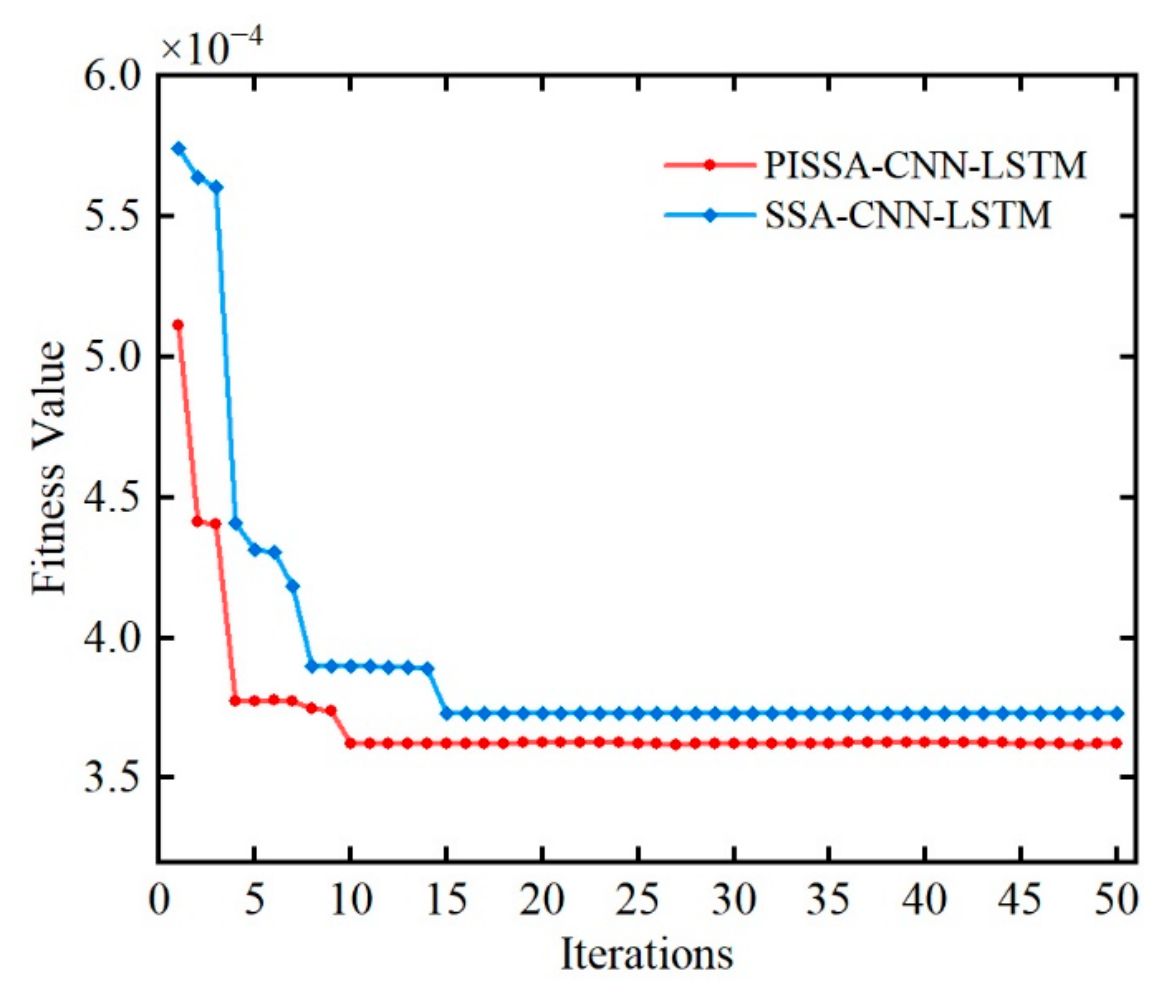
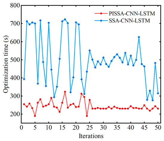
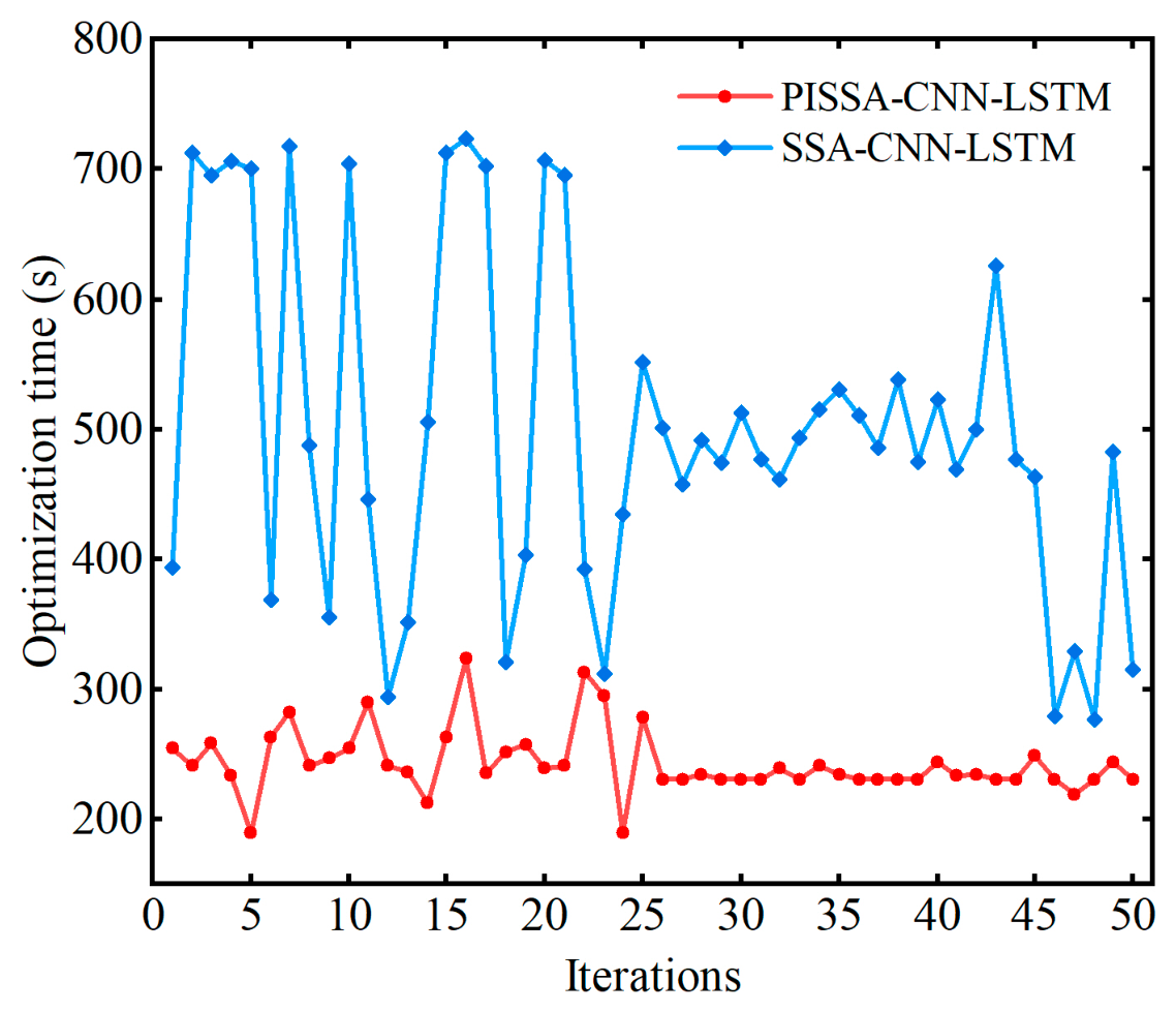
To explain why PISSA-CNN-LSTM outperforms SSA-CNN-LSTM in predictive performance, Table 4 compares the optimal hyperparameter combinations obtained by the two optimization methods, while Figure 8 and Figure 9 present the convergence characteristics and differences in optimization time. Both methods identify a single-layer LSTM as the optimal structure, indicating that a single-layer architecture is sufficient to capture the key temporal dependencies in the friction coefficient sequence, whereas increasing the number of layers may lead to overfitting and increased computational cost. PISSA-CNN-LSTM obtains a larger number of hidden units and a larger batch size, which is consistent with the physics-informed constraint mapping described above. Under complex operating conditions with high current and high sliding speed, interfacial arcing, vibration-induced impacts, and high-frequency random disturbances intensify simultaneously, causing the friction coefficient signal to exhibit stronger fluctuations and higher nonlinear complexity. Therefore, greater model representational capacity and more stable gradient estimates are required. In addition, the learning rate and L2 regularization coefficient of PISSA-CNN-LSTM are also higher than those of SSA-CNN-LSTM, indicating that, within the feasible search space reconstructed by physical constraints, the optimization process is more likely to identify a hyperparameter combination that balances convergence efficiency and generalization capability.
Table 4.
Optimal hyperparameter combinations of the models.
Figure 8.
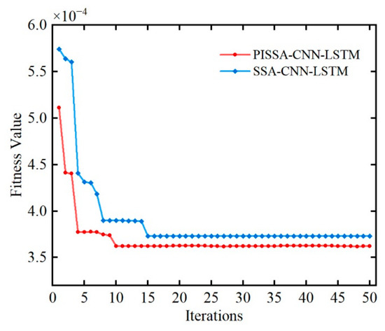
Convergence curves of PISSA-CNN-LSTM and SSA-CNN-LSTM.
Figure 9.
Optimization time curves of PISSA-CNN-LSTM and SSA-CNN-LSTM.
As shown in Figure 8, PISSA-CNN-LSTM reaches the optimal fitness value at the 10th iteration, whereas SSA-CNN-LSTM reaches its optimum at the 15th iteration and then stagnates, suggesting that the latter is more likely to become trapped in a local optimum. Figure 9 shows that the average optimization time for PISSA-CNN-LSTM is 246.94 s, compared with 487.92 s for SSA-CNN-LSTM, corresponding to an efficiency improvement of 49.38%. These results demonstrate that physics-informed constraints can guide the algorithm toward more reasonable hyperparameter combinations while narrowing ineffective search regions and improving the targeted nature of the search direction, thereby enabling faster convergence and higher optimization efficiency.
4.3. Robustness and Statistical Significance Analysis
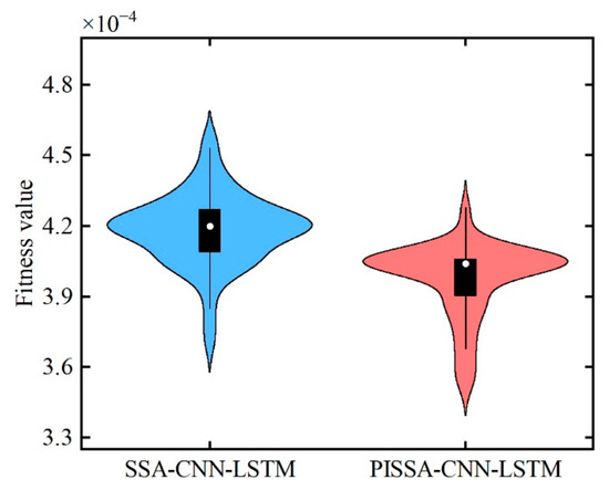
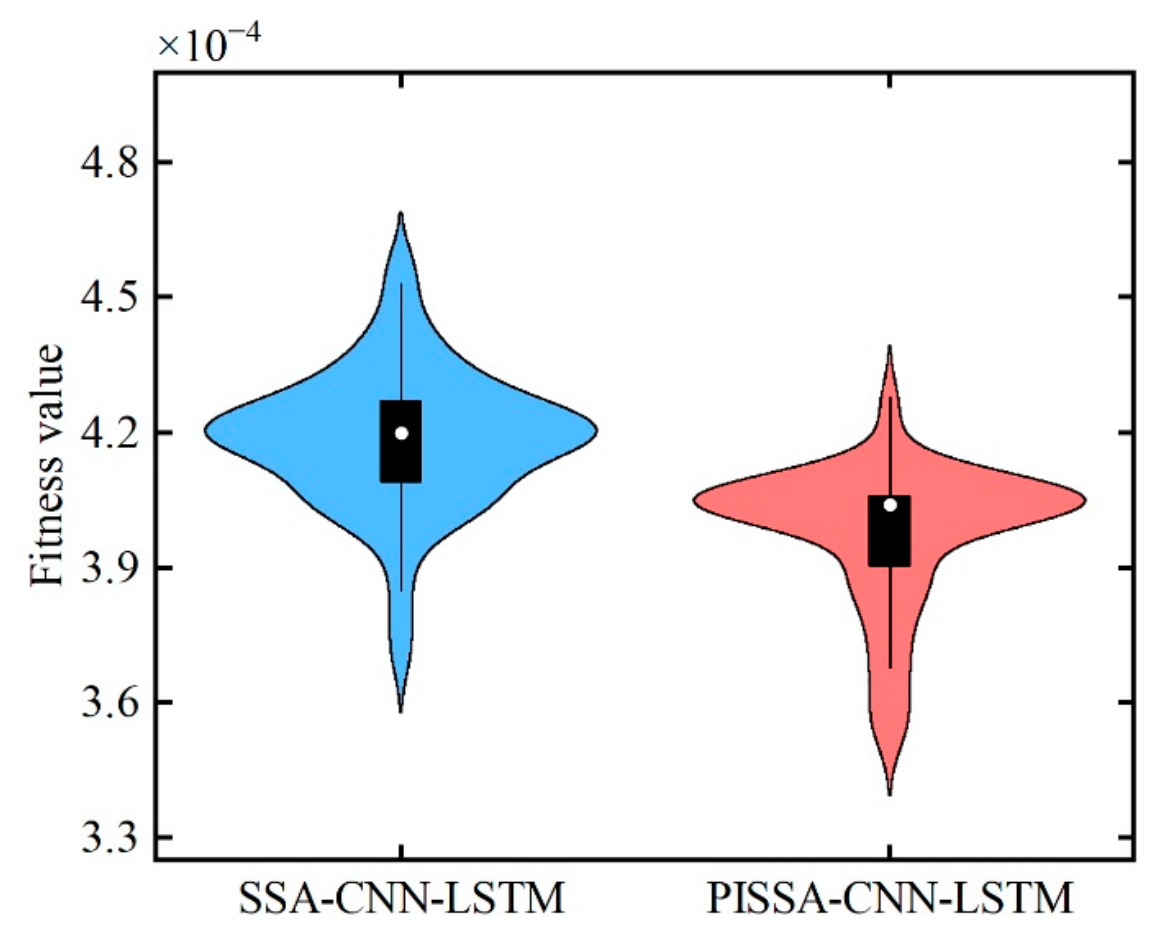
Considering the stochastic nature of swarm intelligence algorithms, the optimal hyperparameter combinations listed in Table 4 were used to conduct 100 independent repeated trials for the CNN-LSTM models optimized by the two methods. The resulting RMSE distributions were then used to evaluate model robustness. As shown in Figure 10, the RMSE distribution of PISSA-CNN-LSTM is generally lower than that of SSA-CNN-LSTM and exhibits smaller variability. The mean RMSE values of PISSA-CNN-LSTM and SSA-CNN-LSTM are 3.9741 × 10⁻⁴ and 4.1842 × 10⁻⁴, respectively, indicating that PISSA-CNN-LSTM achieves a lower average prediction error and better stability.
Figure 10.
Violin plots for different optimal hyperparameters.
To further verify the significance of the performance difference between the two models, a Wilcoxon rank-sum test was performed on the RMSE distributions. The null hypothesis H0 was defined as “the two sample distributions do not differ significantly.” The test results show that p = 3.6647 × 10⁻⁴ < 0.05; therefore, the null hypothesis is rejected, indicating a statistically significant difference between the RMSE distributions of the two models. These results demonstrate that PISSA-CNN-LSTM outperforms SSA-CNN-LSTM in predictive performance, and that its performance improvement is both stable and statistically significant.
5. Potential Extensions and Applications
The proposed model has been validated for the C/Cu contact pair within the range of operating conditions considered in the present tests and has demonstrated strong capability in predicting dynamic friction behavior. By dynamically reconstructing the hyperparameter search boundaries according to operating conditions, PISSA incorporates operational information—including current, contact load, and sliding speed—into the optimization process. Therefore, it does not depend on a specific combination of operating conditions and has the potential to be extended to a broader operating-condition range. For substantially expanded operating domains or different material systems, the boundary-mapping coefficients can be recalibrated using representative data. With the further incorporation of state variables such as dynamic contact resistance, interfacial temperature, and surface morphology, this method could be extended to additional contact-pair materials and current-carrying friction systems, thereby providing a unified framework for the comprehensive prediction and evaluation of the electrical and tribological states of the interface.
6. Conclusions
This study addresses the dynamic prediction of the friction coefficient of pantograph carbon strips under current-carrying operating conditions and proposes a PISSA-CNN-LSTM model based on physics-informed Sparrow Search optimization. The main conclusions are as follows:
- (1)
- Increasing the current reduces the mean friction coefficient while intensifying its fluctuations. Increasing the contact load reduces both the mean value and the fluctuation amplitude of the friction coefficient. In contrast, increasing the sliding speed causes both the mean value and the fluctuation intensity of the friction coefficient to increase simultaneously. The friction coefficient sequence exhibits strong nonlinearity, non-stationarity, and operating-condition dependence, providing a basis for constructing a physics-informed search space.
- (2)
- PISSA-CNN-LSTM maps operating-condition parameters to hyperparameter search boundaries, thereby enabling the transition from black-box optimization to physics-informed guided search. Under the validation operating condition, PISSA-CNN-LSTM reaches the optimal fitness value at the 10th iteration, whereas SSA-CNN-LSTM stagnates at the 15th iteration. The average optimization time of PISSA-CNN-LSTM is 246.94 s, which is 49.38% shorter than that of SSA-CNN-LSTM. On the test set, PISSA-CNN-LSTM achieves an R2 of 0.9904, an RMSE of 3.6479 × 10⁻⁴, an MAE of 3.0009 × 10⁻⁴, and a MAPE of 0.0609%, outperforming the comparative models in all metrics.
- (3)
- In 100 repeated trials, the RMSE distribution of PISSA-CNN-LSTM lies at lower values and exhibits smaller dispersion. The Wilcoxon test yields p = 3.6647 × 10⁻⁴ < 0.05, indicating that the performance improvement is statistically significant. The hyperparameter comparison shows that PISSA-CNN-LSTM obtains a larger number of hidden units, a larger batch size, a higher learning rate, and a larger L2 regularization coefficient, which is consistent with the physics-based rationale that higher model capacity is required under high-current and high-speed operating conditions. This strategy can effectively narrow ineffective search regions and improve both optimization efficiency and predictive robustness.
Author Contributions
J.C.: writing—original draft, conceptualization. G.G.: methodology, funding acquisition. G.W.: funding acquisition, supervision. Q.W.: data curation. G.H.: investigation. R.F.: project administration, visualization. H.W. and T.L.: software, P.Q.: investigation, validation. All authors have read and agreed to the published version of the manuscript.
Funding
This research was funded by the Innovation Research Group Project of the Natural Science Foundation of Sichuan (award No. 2024NSFTD0009) and the Youth Science and Technology Foundation of Gansu (No. 23JRRA828).
Data Availability Statement
The data presented in this study are available on request from the corresponding author. The data are not publicly available due to the relevant research confidentiality requirements.
Acknowledgments
The authors acknowledge the support from Southwest Jiaotong University for providing the experimental facilities.
Conflicts of Interest
The authors declare no conflicts of interest.
Abbreviations
The following abbreviations are used in this manuscript:
| CNN | Convolutional neural network |
| LSTM | Long short-term memory |
| CNN-LSTM | Hybrid model combining CNN and LSTM |
| SSA | Sparrow search algorithm |
| PISSA | Physics-informed Sparrow search algorithm |
| PISSA-CNN-LSTM | CNN-LSTM model optimized by physics-informed SSA |
| Ytrain | Training output dataset |
| Ytest | Testing output dataset |
| y | Actual output value |
| R2 | Coefficient of determination |
| RMSE | Root mean square error |
| MAE | Mean absolute error |
| MAPE | Mean absolute percentage error |
| p | Significance probability in the Wilcoxon rank-sum test |
References
- Wu, G.N.; Dong, K.L.; Xu, Z.L.; Xiao, S.; Wei, W.F.; Chen, H.; Li, J.; Huang, Z.; Li, J.; Gao, G.; et al. Pantograph–catenary electrical contact system of high-speed railways: Recent progress, challenges, and outlooks. Railw. Eng. Sci. 2022, 30, 437–467. [Google Scholar] [CrossRef] [Scilit]
- Gao, G.Q.; Qian, P.Y.; Xu, Z.L.; Dong, K.L.; Wang, Q.S.; Peng, W.; Liu, Y.; Ma, Y.; Xiao, S.; Huang, G.; et al. The evolution law of the pantograph–catenary arc with the multi-stress coupled force analysis under the sub-atmospheric pressure strong-airflow condition. Phys. Plasmas 2023, 30, 053502. [Google Scholar] [CrossRef] [Scilit]
- Zhi, X.S.; Zhou, N.; Wei, H.F.; Chen, H.M.; Cheng, Y.; Sun, Y.; Zhao, L.; Huang, G.; Zhang, W. Analysis of the abnormal wear of the pantograph contact strip through combined experimental and simulation approaches. Sci. Rep. 2025, 15, 45706. [Google Scholar] [CrossRef] [Scilit] [PubMed]
- Luo, Q.; Bruni, S.; Bucca, G.; Mei, G.M.; Chen, G.X.; Zhang, W.H. Wear performance of pantograph–overhead catenary system: A review. Railw. Eng. Sci. 2026, 1–20. [Google Scholar] [CrossRef] [Scilit]
- Wang, P.; Wei, F.C.; Zhao, Z.W.; Guo, Y.G.; Du, S.M.; Hao, Z.H. Effect of heat treatment temperature on mechanical and tribological properties of copper impregnated carbon/carbon composite. Tribol. Int. 2021, 164, 107209. [Google Scholar] [CrossRef] [Scilit]
- Zhi, X.S.; Zhou, N.; Cheng, Y.; Wei, H.F.; Yao, Y.M.; Zhang, W.H.; Chen, G. Study on wear performance and mechanism of pantograph contact strip that contact with damaged contact wire under ambient humidity. Friction 2026, 14, 9441101. [Google Scholar] [CrossRef] [Scilit]
- Gao, G.Q.; Fu, R.; Wang, Q.S.; Chen, J.H.; Qian, P.Y.; Zeng, J.J.; Weng, X.; Li, H.; Yang, Z.; Wang, H.; et al. Progress on current-carry friction and wear and prediction models: A review. Friction 2025, 14, 9441151. [Google Scholar] [CrossRef] [Scilit]
- Fu, Y.; Qin, H.; Xu, X.; Zhang, X.; Guo, Z. What are the Progresses and Challenges, from the Electrical Properties of Current-Carrying Friction System to Tribological Performance, for a Stable Current-Carrying Interface? J. Bio Tribo Corros. 2022, 8, 4. [Google Scholar] [CrossRef] [Scilit]
- Song, J.Y.; Dong, C.L.; Bai, X.Q.; Yuan, C.Q. Friction-coefficient prediction and wear-state diagnosis of rotary-vane steering gear seals using CNN-LSTM and LightGBM. Tribol. Int. 2025, 212, 110991. [Google Scholar] [CrossRef] [Scilit]
- Yin, F.L.; He, Z.Z.; Nie, S.L.; Ji, H.; Ma, Z.H. Tribological properties and wear prediction of various ceramic friction pairs under seawater lubrication condition of different medium characteristics using CNN-LSTM method. Tribol. Int. 2024, 189, 108935. [Google Scholar] [CrossRef] [Scilit]
- Xue, J.K.; Shen, B. A survey on sparrow search algorithms and their applications. Int. J. Syst. Sci. 2024, 55, 814–832. [Google Scholar] [CrossRef] [Scilit]
- Hosseinzadeh, M.; Andriani, D.P.; Rahmani, A.M.; Gharehchopogh, F.S.; Rahimi, N.; Khan, A.; Darwesh, A.; Khoshvaght, P.; Din, S.; Porntaveetus, T. A Comprehensive Survey of SSA-LSTM Models: Signal Decomposition Techniques, Algorithmic Advances, Practical Applications, and Future Directions. Arch. Comput. Methods Eng. 2026. [Google Scholar] [CrossRef] [Scilit]
- Wu, J.P.; Zhao, P.; Cui, J.H.; Wang, L.Y.; Yang, C.B.; Ouyang, J.P. Data-Driven Prediction of Coefficient of Friction in Wet Friction Components: A Model Development and Interpretability Analysis. J. Tribol. 2025, 147, 074601. [Google Scholar] [CrossRef] [Scilit]
- Xia, Y.Q.; Zhao, H.B.; Feng, X. Prediction of grease performance and optimal additive ratio based on the SSA-GDA-LSSVM model. Tribol. Int. 2025, 202, 110366. [Google Scholar] [CrossRef] [Scilit]
- Zhu, K.P.; Huang, C.Y.; Li, S.; Lin, X. Physics-informed Gaussian process for tool wear prediction. ISA Trans. 2023, 143, 548–556. [Google Scholar] [CrossRef] [Scilit] [PubMed]
- Kovalev, A.; Tian, Y.; Meng, Y.G. Prediction of ball-on-plate friction and wear by ANN with data-driven optimization. Friction 2024, 12, 1235–1249. [Google Scholar] [CrossRef] [Scilit]
- Pashmforoush, F.; Araghizad, A.E.; Budak, E. Physics-informed tool wear prediction in turning process: A thermo-mechanical wear-included force model integrated with machine learning. J. Manuf. Syst. 2024, 77, 266–283. [Google Scholar] [CrossRef] [Scilit]
- Zeng, Y.C.; Song, D.L.; Zhang, W.H.; Zhou, B.; Xie, M.Y.; Tang, X. A new physics-based data-driven guideline for wear modelling and prediction of train wheels. Wear 2020, 456–457, 203355. [Google Scholar] [CrossRef] [Scilit]
- Yang, Y.; Wu, X.Y.; Yu, J.B.; Wang, Y.S.; Sun, X.W. Simulation analysis of slip rings based on archard model. Ind. Contr. Comput. 2019, 32, 107–108+139. (In Chinese) [Google Scholar]
- Wang, H. Research on the Influence of Interface Oxidation on the Characteristics of Friction and Wear of Carbon–Copper Electrical Sliding Contacts. Ph.D. Thesis, Southwest Jiaotong University, Chengdu, China, 2022. [Google Scholar] [CrossRef]
- Ren, W.B.; Zhang, X.; Meng, X.X. Fretting behavior of gold-plated contact materials used in high-frequency vibration and different temperature environment. IEEE Trans. Compon. Packag. Manuf. Technol. 2017, 7, 572–581. [Google Scholar] [CrossRef] [Scilit]
- Mei, G.M.; Fu, W.M.; Chen, G.X.; Zhang, W.H. Effect of high-density current on the wear of carbon sliders against Cu-Ag wires. Wear 2020, 452, 203275. [Google Scholar] [CrossRef] [Scilit]
- Zhao, H.; Feng, Y.; Zhou, Z.J.; Qian, G.; Zhang, J.C.; Huang, X.C.; Zhang, X. Effect of electrical current density, apparent contact pressure, and sliding velocity on the electrical sliding wear behavior of Cu-Ti3AlC2 composites. Wear 2020, 444–445, 203156. [Google Scholar] [CrossRef] [Scilit]
- Li, K.M.; Shang, G.B.; Du, S.M.; Zhang, Y.Z. Effects of friction velocity and current density on current-carrying friction and wear properties of copper matrix composites. Mech. Eng. Mater. 2015, 39, 22–27. (In Chinese) [Google Scholar]
- Shen, M.X.; Ji, D.H.; Hu, Q.; Xiao, L.; Li, Q.P. Current-carrying tribological behavior of C/Cu contact pairs in extreme temperature and humidity environments for railway catenary systems. Sci. China Technol. Sci. 2024, 67, 2537–2548. [Google Scholar] [CrossRef] [Scilit]
- Bouchoucha, A.; Chekroud, S.; Paulmier, D. Influence of the electrical sliding speed on friction and wear processes in an electrical contact copper-stainless steel. Appl. Surf. Sci. 2004, 223, 330–342. [Google Scholar] [CrossRef] [Scilit]
- Yang, Z.H.; Shang, G.B.; Sun, L.M.; Zhang, Y.Z. Effect of relative sliding velocity on current-carrying friction properties of copper-graphite composites. J. Henan Univ. Sci. Technol. 2021, 42, 1–6+117. (In Chinese) [Google Scholar] [CrossRef] [Scilit]
- Wang, L.; Hu, D.C. Study on arc erosion resistance of C/C composites. J. Chin. Soc. Corros. Prote 2009, 29, 235–240. (In Chinese) [Google Scholar]
- Chen, T.H.; Song, C.F.; Zhang, Y.Y.; Niu, K.; Liu, Z.L.; Wang, L.; Sun, C.; Li, M.; Zhang, Y. Current-carrying contact character and wear behavior of an elastic ring at different rolling speeds. Eng. Fail Anal. 2022, 131, 105825. [Google Scholar] [CrossRef] [Scilit]
- Li, C.H.; Zhang, Y.Y.; Ceng, Z.X.; Niu, K.; Song, C.F.; Shang, G.B.; Zhang, Y.Z. Research progress of current-carrying friction and wear. Lubr. Eng. 2022, 47, 153–167. (In Chinese) [Google Scholar]

Disclaimer/Publisher’s Note: The statements, opinions and data contained in all publications are solely those of the individual author(s) and contributor(s) and not of MDPI and/or the editor(s). MDPI and/or the editor(s) disclaim responsibility for any injury to people or property resulting from any ideas, methods, instructions or products referred to in the content. |
© 2026 by the authors. Licensee MDPI, Basel, Switzerland. This article is an open access article distributed under the terms and conditions of the Creative Commons Attribution (CC BY) license.