


Abstract
Tool wear degrades machining quality and, if unchecked, can progress to breakage, causing workpiece defects, downtime, and spindle damage; automatic tool condition monitoring is therefore essential. In real production, new and reground tools are used interchangeably and differ slightly in geometry and material, so the “normal” baseline shifts from one tool and mounting to the next. This makes both global-baseline diagnostics and deep-learning methods that require large labeled fault datasets difficult to apply. This study proposes a lightweight, self-referencing framework—whose per-tool baseline is built from acceptable-state data alone—for diagnosing milling tool wear under tool-to-tool variability. Its novelty lies not in the individual techniques—self-referencing, order tracking, and the Mahalanobis distance, which are established—but in their integration into a single framework, designed for fault-label-free operation, that rebuilds a dedicated baseline for every newly mounted tool. Whenever a tool is mounted, its own acceptable data, a short initial segment of machining taken as healthy immediately after mounting, form the baseline; kinematics-based order-tracked features from a single spindle-bearing accelerometer are used to compute the Mahalanobis distance from the acceptable state, which serves as a continuous health index. A warning limit set statistically from the acceptable data alone, together with a defect limit set as a pragmatic engineering multiple of it, separates the acceptable, warning, and defect grades. On four end mills of identical specification, the primary full-baseline analysis yielded a warning-detection AUC of 0.986 and a defect-detection AUC of 0.936; with a persistence rule, defect-grade wear was detected in all four tools with no false alarms in the acceptable state. Because the baseline is built from only a short acceptable segment and the computation is inexpensive, the framework is, in principle, suited to shop floors with frequent tool changes and to on-machine or edge deployment (not yet benchmarked on an edge device); the present validation, however, is limited to four tools and a single workpiece material under fixed cutting conditions with accelerated wear, so broader verification remains necessary.
1. Introduction
In cutting processes, the tool is a consumable part that wears gradually with use; in severe cases this leads to degraded dimensional and surface quality and to unexpected tool breakage, causing direct losses such as rework and unplanned downtime [1,2]. Because such incidents incur not only direct tool and equipment costs but also productivity losses from unexpected stoppages, real-time tool condition monitoring and timely tool replacement are important tasks in smart manufacturing [2,3]. Accordingly, tool condition monitoring (TCM) using a variety of signals has been studied extensively [4,5,6,7].
The main sensing signals used for TCM—cutting force, spindle current/power, acoustic emission, and vibration—differ markedly in what they capture and in how practical they are to deploy, each entailing trade-offs between sensitivity and shop-floor deployability. Cutting-force (dynamometer) signals are the most directly related to the wear process and are highly sensitive, but they require a table- or spindle-mounted dynamometer that is expensive and intrudes on the machining setup, limiting their use in production [8,9,10]. Spindle-current/power signals can be obtained from the machine drive at low cost without disturbing the machining setup, yet they are comparatively insensitive to incipient wear and to the high-frequency cutting dynamics that carry early wear information [11,12,13]. Acoustic emission (AE) is very sensitive to micro-fracture and chip formation, but it demands very high sampling rates and is strongly affected by wave attenuation, mounting location, and background noise [14,15,16]. Vibration offers a favorable compromise for shop-floor TCM: accelerometers are inexpensive and easy to retrofit, and, mounted on the spindle-bearing housing, they sensitively capture the cutting excitation while remaining comparatively robust to installation variability [17,18,19,20,21]. For these reasons—low cost, ease of installation, and sensitivity to cutting dynamics—the present study adopts a single spindle-bearing accelerometer as the sensing source [5,6].
In vibration-based TCM, features are extracted from time-domain statistics, frequency spectra, and time–frequency representations and related to the wear state [18,22,23]; in particular, changes in the amplitude of the tooth-passing frequency and its harmonics have been reported to be closely related to wear [22,24]. Recently, representations obtained by the wavelet packet transform or the short-time Fourier transform have been fed to deep neural networks to classify or predict wear [25,26,27,28,29,30]. This deep-learning trend continues in current milling studies, including hybrid deep models published in this journal for remaining-useful-life prediction of milling cutters [28] and recent deep-learning approaches for vibration-based tool condition monitoring in milling [31,32]. In addition, machine-learning approaches that combine in-process cutting-force analysis have been demonstrated for tool wear prediction [33].
However, deep-learning-based approaches require large amounts of labeled fault data and considerable training resources, and the learned models are often less interpretable, making the diagnostic rationale difficult to trace [27,34,35]. More fundamentally, most studies mix all data to learn a single model and a global baseline shared across tools; yet when a tool is remounted or replaced—because of the interchangeable use of new and reground tools, slight tool-to-tool differences in material properties and dimensions, runout and mounting condition, and even changes in machine condition—the baseline of the normal signal itself can shift. Such tool-to-tool variability is largely unavoidable in industrial machining, where tools are frequently replaced, reground, and remounted throughout production, so a global baseline requires recalibration at every tool change and is impractical to maintain. Indeed, recent milling-TCM studies, including those addressing varying workpiece and cutting conditions, still largely assume a fixed reference baseline [36]. Transfer learning and domain adaptation have been attempted to mitigate this [34,37], but they can incur additional computational cost, require target-domain adaptation, and still depend on prior fault data. Meanwhile, novelty-detection TCM that learns only from acceptable data has also been proposed [38], but cases that explicitly address tool-to-tool variability while combining normal-statistics-based threshold setting with interpretable features are rare. Crucially, unlike conventional one-class learning that shares a single baseline across tools, the framework pursued here reconstructs the baseline independently for every newly mounted tool; the present study focuses specifically on this tool replacement and remounting variability, leaving variable-speed and machine-to-machine variation to future work.
This study makes three contributions. We emphasize at the outset that the individual building blocks—self-referencing, order-tracked features, and the Mahalanobis distance—are established techniques, and that the primary contribution of this study is their integration into a self-referencing framework that directly targets tool-to-tool variability. First, it addresses tool-to-tool variability with a lightweight, operationally label-free self-referencing framework rather than deep-learning transfer learning. Because each tool’s baseline is built on the fly from only its initial acceptable data—a short healthy segment recorded immediately after mounting—no global recalibration is needed. Second, it introduces physics-informed features based on spindle-rotation kinematics (order tracking, tooth-to-tooth asymmetry) that detect the early warning stage without deep learning, while remaining physically interpretable and aligned with the underlying rotational kinematics [39,40]. Third, it derives a continuous health index from the covariance of the acceptable data, sets an empirical 95th-percentile warning limit, and applies a pragmatic engineering multiple for the defect limit, so that, after deployment, the method can operate on machine controllers or edge devices without fault labels or dedicated hardware accelerators such as GPUs. Systematic comparisons of feature sets, similarity measures, and spectral representations, together with a leave-one-tool-out comparison of self-referencing and global baselines, are presented to evaluate the proposed framework.
The remainder of this paper is organized as follows. Section 2 describes the experimental setup and data acquisition, the signal representation and feature design, and the self-referencing similarity-based diagnosis and evaluation methods. Section 3 presents the spectral/feature/detector comparisons and the results for grading the health index and applying the persistence rule. Section 4 and Section 5 discuss the results and conclude.
2. Materials and Methods
2.1. Experimental Setup and Data Acquisition
In this study, a milling testbed was constructed to acquire vibration data—including tool-to-tool variability—for four different end mills of identical specification. The overall configuration of the testbed and the mounting location of the accelerometer are shown in Figure 1. The testbed was a benchtop three-axis CNC (Mach3 Version 3.043.062-controlled, stepper-driven X/Y/Z axes, working volume 390 × 590 × 75 mm) equipped with a 2.2 kW air-cooled spindle (Ø80 housing, ER20 collet)—a three-phase AC induction motor rated for 24,000 rpm at 400 Hz, with no encoder. The spindle is driven by a variable-frequency drive in open-loop (V/f) mode without closed-loop speed feedback, so the commanded speed is set but not actively regulated to remain constant under cutting load. The tool used was a two-flute HSS end mill with a diameter of 8 mm, a shank diameter of 8 mm, a flute length of 20 mm, and an overall length of 70 mm (Figure 2a, Table 1). A 60 × 60 × 40 mm aluminum block was used as the workpiece (Figure 2b). A two-flute (double-tooth) end mill was used, which is a standard configuration for small-diameter (8 mm) HSS end mills and, in particular, for slot milling of aluminum, where the larger per-tooth flute space assists chip evacuation; it thus represents a common machining case. The proposed framework is not specific to this choice: the flute count only determines the tooth-passing order (here TPF = 2 × 1X), and the order-tracked features—here, for the two-flute cutter, odd orders capture the rotational family and even orders the tooth-passing family—extend in concept to other flute counts, provided the order grouping is reformulated according to the tooth count. The study targets the vibration-signal characteristics of tool wear and the detection method built upon them rather than the machining of a specific material; aluminum, a widely machined industrial material, was used as a representative and readily machinable workpiece on the present testbed, and the feature construction is primarily kinematics-based, although the resulting feature distributions and control limits may remain material-dependent.
Figure 1.
Components of the milling testbed and the mounting location of the accelerometer (500 mV/g).
Figure 2.
(a) The two-flute HSS end mill used in the experiment and (b) the aluminum workpiece (60 × 60 × 40 mm).
Table 1.
Specifications of the end mill used in the experiments.
Machining for data acquisition was performed as follows. Under up-cutting conditions with a commanded spindle speed of 12,000 rpm and a feed rate of 300 mm/min (approach feed 70 mm/min), the aluminum surface was machined along straight paths at a depth of 1 mm (line-by-line, Figure 3), and a total of 15 straight-cut passes were repeated per state. To measure close to the source of cutting excitation (the cutting point), an accelerometer with a sensitivity of 500 mV/g was attached to the spindle-bearing housing (Figure 1), and signals were acquired at 25,600 Hz and stored as 1 s frames.
Figure 3.
Example of line-by-line machining.
The wear stages were induced artificially by drilling into a concrete block (Figure 4). First, a brand-new, never-used end mill was mounted and used for 15 straight-cut passes at 1 mm depth, acquired as the Normal state. Then, for Wear Stage 1, the tool was worn by drilling into the concrete block to a depth of 1 mm, after which the same 15 straight cuts were repeated; for Wear Stages 2 and 3, data were acquired after drilling the concrete block to depths of 2 mm and 3 mm, respectively. This procedure was repeated for each of four different end mills—four runs in total—to build the dataset. The dataset was acquired on a shared laboratory milling testbed, and the same data were also used in a deep-learning-based wear-severity classification study [41]. These Wear 1/2/3 levels are induced degradation stages defined operationally by the concrete-drilling depth (1/2/3 mm); they are not calibrated against a quantitative flank-wear measure such as the ISO 8688 [42] flank wear (VB). Throughout this paper, “Normal” and “Wear 1/2/3” therefore denote induced, ordinally ordered degradation stages, whereas “flank wear (VB)” is reserved for quantitatively measured wear; the diagnosis relies only on the monotonic ordering of these induced stages within each tool, not on their absolute wear magnitude.
Figure 4.
Method for inducing the wear stages (concrete-drilling depth of 1/2/3 mm).
As noted in the Introduction, such tool-to-tool and mounting-to-mounting differences—including runout at mounting, i.e., eccentric wobble of the tool about the axis of rotation—can shift the normal-signal baseline even for new tools of identical specification. Therefore, in this study each of the four tools was treated as an independent case and data were not mixed across tools. In addition, the machined surface of each state was photographed and used as an independent reference for wear severity. The machined surface remained clean at the Normal and Wear 1 stages, became somewhat rough at Wear 2, and was clearly damaged at Wear 3; this machined-surface quality was used as an independent qualitative cross-check of the vibration-based health index described later.
2.2. Cutting-Segment Extraction and Verification of Wear Progression
Each acquisition run is about 230 s long and consists of 15 machining passes and the tool-transit intervals between them. In this study, one 1 s frame is taken as a single observation; in each state, 15 cutting passes are detected from the peaks of the RMS envelope, and only the central 4 s of stable cutting of each pass is taken (Figure 5). This excludes the entry/exit transients and the tool-transit intervals, yielding an identical 15 × 4 = 60 cutting observations regardless of tool or state. The 15 passes were located by peak detection on the median-filtered per-frame RMS envelope, and the four 1 s frames centered on each detected peak were retained as that pass’s observations. For reproducibility, the per-frame RMS envelope was smoothed with a length-3 median filter (three consecutive 1 s frames), and passes were identified with a peak-detection criterion requiring a minimum inter-peak spacing of 7 frames and a prominence of at least 20% of the maximum smoothed RMS; the first 15 detected peaks were retained, each defining the 4 s (four-frame) window centered on the peak.
Figure 5.
Cutting-segment resampling (example of a normal signal). Fifteen cutting passes are detected from the RMS envelope, and only the central 4 s stable-cutting window (shaded) of each pass is used as an observation.
Because the wear stages are specified by the concrete-drilling depth (0/1/2/3 mm), the labels are already known by experimental design; the Wear 2 and Wear 3 (fault-stage) labels are used for evaluation and for the physical validation below; the baseline and warning limit are built from acceptable-state data (Normal and Wear 1) alone, whereas the defect limit is a pragmatic engineering multiple of the warning limit, calibrated with reference to the wear data (Section 4) and adjustable to site-specific quality tolerances in deployment. To confirm that the artificially induced wear actually causes physically meaningful progression, two expected trends were checked in the data (Figure 6). First, the spindle speed estimated from the first rotational harmonic was 12,007 rpm in the Normal state, almost identical to the commanded value, and decreased monotonically as wear progressed, dropping to about 11,650 rpm at Wear 3. Because the spindle is driven in open-loop (V/f) mode without closed-loop speed regulation (Section 2.1), its actual speed is not held constant under load; the ~3% reduction is therefore consistent with load-induced droop (increased induction-motor slip) as the cutting load rises with wear. This reported speed is estimated from the first rotational harmonic (1X) of the vibration signal rather than from an encoder, and because no cutting force or torque was measured directly, the load–droop link is presented as an indirect (though physically expected) interpretation. Crucially, the estimated 1X is used only to position the order-tracking windows (Section 2.3), so the diagnosis does not depend on the cause of the speed change—indeed, this speed variation is precisely what motivates order tracking. Second, the cutting RMS increased monotonically as wear progressed. Both trends appeared consistently across the four tools, confirming that the assigned wear stages correspond to a physically monotonic progression in severity.
Figure 6.
Spindle rotational speed (a) and cutting RMS (b) versus wear stage for each tool.
A closer inspection of Figure 6b shows that the four tools differ not only in their baseline RMS levels but also in the rate and shape of the wear-induced RMS increase. Tool 1 rises at an approximately constant rate, and Tool 2 nearly saturates between Wear 2 and Wear 3. Tools 3 and 4 behave differently: from Normal to Wear 1 they increase comparably to Tools 1 and 2, from Wear 1 to Wear 2 they rise more weakly than Tools 1 and 2, and from Wear 2 to Wear 3 they increase comparatively sharply. Tool 4 shows the steepest final increase—a delayed but sharp progression. This per-tool divergence is robust to the choice of central tendency—the same pattern is obtained when each point is computed as the median instead of the mean of the stable-cutting segments—indicating that it reflects genuine tool-to-tool variability rather than an averaging artifact, consistent with the final-state edge images in Figure 7. Because the cutting RMS is used here only to characterize the wear stages and not as a diagnostic feature, this heterogeneity in both level and trajectory is precisely why a single global RMS threshold cannot grade all tools consistently; it motivates the self-referencing index adopted in this work, which evaluates each tool against its own acceptable baseline (Normal and Wear 1).
Figure 7.
(a) Microscopic bottom-face (end-face) images of the cutting edge at each wear stage. The red outlines indicate the worn edge region, which expands from Normal to Wear 3, consistent with the signal-based wear progression in Figure 6. (b) Side (peripheral/corner) views of the end mills: The unused (Normal) tool and the four tools at the final Wear 3 state (Exp. 1–Exp. 4). The corner region where the end and peripheral cutting edges meet—the region engaged during the shallow (1 mm) slot milling—shows wear and edge damage in all four worn tools, complementing the bottom-face microscopy of (a).
The progressive wear of the cutting edge itself was likewise confirmed by microscopy, expanding from Normal to Wear 3 (Figure 7a). The per-stage cutting-edge images in Figure 7a were taken on a separate end mill dedicated to imaging, which was subjected to the same concrete-drilling protocol and photographed at each wear stage. Because the four end mills used for the vibration measurements were deliberately kept mounted throughout data acquisition to preserve each tool’s mounting condition, the per-stage imaging was performed on the separate dedicated tool rather than on the measurement tools; the final worn states of the measurement tools themselves are shown in Figure 7b and are consistent with the progression documented in Figure 7a. The concrete-drilling step loads the end (bottom) cutting edges and the adjacent corner most directly; because the aluminum was subsequently slot-milled at an axial depth of only 1 mm, the region engaged in cutting is the bottom corner and the lowest ~1 mm of the peripheral (side) cutting edge—the same region where the drilling-induced damage concentrates. Side (peripheral/corner) views of the unused tool and of the four tools at the final Wear 3 state (Figure 7b) show that this corner/peripheral cutting-edge region is degraded in all four tools, with the damage concentrated at the tip/corner rather than along the full flute length.
2.3. Signal Representation and Kinematics-Based Feature Design
Rather than feeding the raw signal directly into a data-dependent model, the features were designed from known cutting kinematics so as to preserve the interpretability of the method and to remain applicable when field data are scarce. The feature design rests on the following three choices.
Spectral representation: First, three standard representations—the acceleration amplitude spectrum, the velocity spectrum, and the acceleration envelope spectrum—were compared under the same diagnostic pipeline. The acceleration amplitude spectrum performed best (Section 3), which is also physically reasonable: tool wear increases both the tooth-passing components and the broadband floor, and the acceleration spectrum represents these directly (representative spectra in Figure 8). Therefore, in this study all features were extracted from the acceleration amplitude spectrum obtained by a discrete Fourier transform with a Hann window applied to each 1 s frame.
Figure 8.
Acceleration spectra by wear state (Exp. 1); each panel is the mean spectrum of one state. Peaks are labeled as the rotational frequency (1X, with its estimated value annotated in each panel) and its odd rotational harmonics (3 × 1X, 5 × 1X), together with the tooth-passing frequency of the two-flute cutter (TPF = 2 × 1X) and its harmonics (TPF × 2, TPF × 3). As wear progresses, the estimated 1X frequency decreases (from about 200 Hz to 194 Hz) as the estimated spindle speed decreases (consistent with load-induced droop)—i.e., the peaks shift toward lower frequency—which is why order tracking is required. Because TPF = 2 × 1X is an exact multiple of the rotational frequency, the first-order tooth-passing sidebands (TPF ± 1X) coincide with the rotational harmonics (1X and 3 × 1X) and are not spectrally separable. Wear appears mainly as an increase in the tooth-passing (2 × 1X) amplitude—becoming comparable to or larger than 1X in the worn states—and a rise in the broadband floor, whereas the individual higher harmonics do not increase uniformly.
1X rotational-speed estimation gate: Because the spindle speed varies with wear, placing windows at fixed nominal frequencies would gradually miss the shifted harmonics, with the error growing for higher-order harmonics. Computed order tracking provides a standard means of aligning spectral components with variations in rotational speed [39,40]. In the present implementation, each observation passes through a 1X rotational-speed estimation gate (Figure 9), in which the peak within the 1X band (185–207 Hz) of the velocity spectrum is refined using three-point parabolic interpolation to estimate the actual rotational frequency. The velocity spectrum is used at this step because integrating the acceleration (a 1/f weighting in the frequency domain) suppresses high-frequency content and emphasizes the low-order rotational component, giving a cleaner, more reliable 1X peak; all diagnostic features are nonetheless extracted from the acceleration amplitude spectrum. Concretely, it is estimated as
where is the center frequency of the peak bin k within the 1X band, the spectral amplitude at bin k, and Δf the frequency bin spacing. The gate accurately recovers the spindle speed and tracks its decrease with wear (Figure 6); the rotational frequency used for label verification is also obtained from this gate.
Figure 9.
The 1X rotational-speed estimation gate and the order-tracked feature-extraction flow.
Order-tracked features: All harmonic windows are placed at integer (and half-order) multiples of the estimated 1X with a ±10 Hz width—chosen to accommodate the spindle-speed fluctuation while preventing overlap between adjacent harmonics—so the features follow the rotation regardless of speed variation. Because these windows are centered on multiples of the per-observation estimated 1X (order tracking), the order-proportional frequency drift is compensated at each order, so a fixed ±10 Hz half-width—much smaller than the spacing between adjacent tracked orders—prevents overlap between neighboring windows while still capturing each harmonic across the order range used (up to 12×). An 11-element feature vector was computed from the acceleration amplitude spectrum X (f) of each observation; the definition and physical meaning of each feature are summarized in Table 2. In brief, it comprises the amplitudes of the 1X, the tooth-passing frequency (TPF), and its second harmonic (2 × TPF); the normalized energies of the even-order (tooth-passing, 2–12×), odd-order (rotation, 1–11×), and half-order (0.5–5.5×) series; the normalized energies of the broadband floor and the high-frequency (3–8 kHz) band; and two ratio indicators (asymmetry and loss of periodicity) together with the spectral centroid. The even-order series targets the tooth-passing component of the two-flute cut, the odd-order series targets tooth-to-tooth asymmetry due to non-uniform wear, the half-order series targets asynchronous instability components such as chatter onset, and the broadband/ratio terms target the loss of periodicity in severe wear. Here the half-order series includes only half-integer multiples of 1X (0.5·1.5·2.5·… × 1X) and, because its ±10 Hz windows do not overlap the integer harmonics (1X, 2X, etc.), it is computed independently of them. The half-order series was limited to the low orders (0.5–5.5×) where instability components concentrate, because higher-order half-order components decay rapidly and overlap the broadband floor, and the high-frequency energy rise in severe wear is handled by the separate high-frequency band (3–8 kHz) and broadband-floor features. These features were defined a priori from cutting kinematics without any data-driven selection, in order to preserve interpretability and avoid overfitting. Thus the number of features (11) is not an optimization target but a consequence of physical-phenomenon coverage, and correlations/redundancy among features are stably absorbed by the Ledoit–Wolf shrinkage covariance. The Ledoit–Wolf estimator is adopted here because the self-referencing baseline uses only a short acceptable segment—a small-sample regime in which the ordinary sample covariance is ill-conditioned—so it yields the numerically stable covariance that the Mahalanobis health index in Section 2.4 requires. In other words, the features were chosen to represent distinct physical mechanisms of milling vibration rather than to maximize statistical performance. The energy of the o-th order band is defined as
and the total energy is used for normalization and defined as
Table 2.
Definitions of the order-tracked features (±10 Hz windows placed at multiples of the estimated 1X; energies referenced to the acceleration amplitude spectrum).
2.4. Self-Referencing Similarity-Based Diagnosis
This diagnosis follows a simple idea consistent with how tools are actually replaced in the field: when a tool is mounted, its initial acceptable data (the data assumed healthy immediately after mounting) are taken as the baseline, and any subsequent state is judged by how similar it is to that baseline. Accordingly, for each tool a baseline distribution is constructed from that tool’s own acceptable data, and how dissimilar a new observation is from that distribution is measured by the Mahalanobis distance.
Construction of the health index: For each tool, the 11-dimensional features (the order-tracked features described in Section 2.3) are standardized using acceptable data from that tool. The shrinkage covariance is estimated using Ledoit–Wolf shrinkage [43] to ensure stability even with limited observations and correlated features:
where S is the sample covariance, p the feature dimension, ρ ∈ [0, 1] the analytically determined shrinkage intensity, tr(·) the trace, and I the identity matrix. The health index for an arbitrary observation x is the Mahalanobis distance to the acceptable distribution, defined as
where μ and Σ are the mean and shrinkage covariance of the acceptable data. This distance is a “dissimilarity from the acceptable state” that reflects the scale and correlation of the features; the smaller the value, the healthier, and the larger, the more worn. Because the health-index baseline for each tool is constructed using only that tool’s acceptable data, no fault data are required to compute the health index. Moreover, the absolute values of the harmonic amplitudes differ across tools (e.g., for some tools the 2 × TPF component can be larger than the TPF even in the normal state), so absolute values themselves are hard to use as diagnostic criteria; but because the method uses each tool’s deviation relative to its own normal state rather than absolute values, such tool-to-tool differences are absorbed during standardization.
Why the Mahalanobis distance was chosen: The Euclidean distance treats all standardized feature directions isotropically and ignores their covariance structure, and the cosine dissimilarity looks only at the direction of the vector and discards its magnitude (energy). However, the order-tracked features in this study have mutually correlated harmonic energies with disparate scales, and much of the wear information is carried in the increase in energy. The Mahalanobis distance (i) normalizes scale and correlation via the covariance, so deviation is measured in units of the local dispersion of the acceptable state and is invariant to feature rescaling; (ii) means that when the normal state follows a multivariate Gaussian distribution, its square corresponds, up to a constant, to the negative log-likelihood, so equidistant contours are exactly iso-probability-density ellipsoids; (iii) estimates the inverse covariance stably even when acceptable samples are limited, due to Ledoit–Wolf shrinkage. These properties directly explain the results in Section 3, in which the cosine measure was essentially random, the Euclidean worked but was inferior, and the Mahalanobis distance was the best.
State grading: To align with machined-surface quality (Normal and Wear 1 good, Wear 2 degraded, Wear 3 poor), Normal and Wear 1 were grouped together as acceptable, Wear 2 as a warning state, and Wear 3 as a defect state. Here “Normal” is a wear label denoting the unworn, new-tool state, whereas “acceptable” denotes the healthy category not requiring replacement (Normal and Wear 1); each tool’s self-referencing distribution is constructed from these acceptable data. Throughout this paper we accordingly keep two distinct vocabularies: “Normal” and “Wear 1/2/3” denote the (induced) physical degradation stages, whereas “acceptable”, “warning”, and “defect” denote the diagnostic classes, with the mapping acceptable = Normal + Wear 1, warning = Wear 2, defect = Wear 3. In this experiment the acceptable data comprise the Normal and Wear 1 observations; in practical deployment, where wear-stage labels are unavailable, the acceptable baseline is instead taken from the initial machining period immediately after mounting a new or reground tool, during which the tool is assumed healthy under the scheduled maintenance policy (Section 4).
Statistical setting of the thresholds: The warning threshold was determined from the health-index distribution of the acceptable data only. The defect threshold was then defined as a pragmatic engineering multiple of the warning limit and evaluated through the sensitivity analysis described below. Following the convention of multivariate statistical process control, the statistical warning limit is set from the distribution of the acceptable index to target a desired false-alarm probability. The theoretical basis is that, if the acceptable features are multivariate Gaussian, the squared distance would, under ideal known population parameters, be exactly -distributed. For an independent future observation, a classical F-based reference distribution can be obtained for the corresponding Mahalanobis-type statistic when the reference mean and covariance are estimated by the ordinary sample mean and covariance under multivariate normality [44,45],
approaching a distribution for large n. Equation (6) summarizes this classical reference relationship and is not used to determine the control limits in the present study. However, because finite samples, shrinkage covariance, and non-normal features can make the actual distribution differ from this (indeed, it did not closely follow the in our data), the statistical warning limit was set from a distribution-free empirical percentile rather than a theoretical quantile. Accordingly, the warning threshold was set at the empirical 95th percentile of the acceptable pass-level index for that tool (each pass value being the mean of its frame health indices, Equation (8); this pass-level aggregation is the quantity used for the operating decision, so the nominal 5% upper-tail probability applies per pass rather than per 1 s frame) (a nominal 95th-percentile warning limit; ≈5% upper-tail probability in the acceptable reference distribution); this percentile was selected as a practical operating point to balance detection sensitivity and false alarms. Since a purely statistical limit (e.g., the 99.7th percentile) alone left the health indices of the warning (Wear 2) and defect (Wear 3) grades overlapping so that the two grades were not separated, the defect threshold was provisionally set as a pragmatic engineering action limit at three times the warning line (Figure 10; the specific multiple is justified below by a 2.5×–3.5× sensitivity analysis). The warning threshold is defined using acceptable data only and requires no fault (Wear 2/3) labels, whereas the defect line is set as a pragmatic engineering multiple of the warning limit whose stability within the tested range is supported by the sensitivity analysis in Table 9; this two-stage limit design is analogous in structure to the warning/action lines (escalating alarm levels) used in statistical process control [44,45]. The defect-line multiple (three times) was not fixed arbitrarily but selected as the median of a wide stable interval over which the tool-level grade diagnosis is unchanged when the multiple is varied between 2.5× and 3.5× (Section 4); the tool-level diagnosis was insensitive to the multiplier within the tested 2.5×–3.5× range. We emphasize that, unlike the statistically grounded warning line, this defect line is a pragmatic engineering action limit supported by the sensitivity analysis (an invariant tool-level grade diagnosis over 2.5×–3.5×; Table 9) rather than derived from a statistical distribution. Machined-surface quality was not used to set the numerical control limits; it informed only the class mapping (grouping Normal and Wear 1 as acceptable) and served as an independent qualitative check that Wear 2 falls in the warning region and Wear 3 in the defect region. Accordingly, for each tool, the warning limit was set independently as the empirical 95th percentile of that tool’s acceptable pass-level health-index distribution,
where is defined in Equation (8) and the defect limit is at = 3 (Section 4). Thus, all tools use the same percentile-and-multiplier rule, whereas the numerical limits are reconstructed from each tool’s own acceptable-state distribution.
Figure 10.
Distributions of the frame-level Mahalanobis health index and the tool-specific warning and defect limits for the four tools. For each tool, the warning limit is the empirical 95th percentile of its own acceptable pass-level mean health-index distribution, and the defect limit is three times the corresponding warning limit.
Persistence rule: For field application, the per-second decisions were aggregated to the machining unit. The pass value is
i.e., the mean of the per-observation indices in that pass.
An alarm was raised only when three consecutive passes exceeded the threshold—a value chosen as a compromise between detection latency and robustness to transient disturbances. Here this three-pass window spans three machining passes (of the order of ten seconds of cutting in the present setup); for processes with substantially different pass durations—such as long passes on large parts or short grinding cycles—the window can be lengthened, shortened, or made adaptive to preserve the same latency–robustness balance. This persistence rule suppresses transient false alarms that can occur in per-second decisions.
2.5. Evaluation Method
Both a threshold-independent view and an operating-point view are presented. The threshold-independent view is the area under the ROC curve (AUC) for two tasks: warning detection (acceptable class vs. Wear 2, excluding Wear 3) and defect detection (acceptable and warning classes vs. Wear 3). Unless otherwise noted, the reported AUCs correspond to this primary full-baseline analysis, in which each tool’s complete acceptable dataset is used to estimate its self-referencing baseline; the five-fold analysis in Section 4 separately assesses sensitivity to acceptable-baseline re-estimation. The operating-point view reports the machining-unit detection results using a warning limit corresponding to a nominal 5% upper-tail probability in the acceptable reference distribution, together with the tool-level results after applying the persistence rule. All fitting—including each tool’s warning and defect limits—was performed within that tool, so that there was no information leakage across tools. Unless noted otherwise, the reported AUCs are pooled across the four tools (evaluated on the combined per-tool self-referenced scores), and per-tool AUCs are additionally given where relevant (Section 3.2).
2.6. Comparative Study
To evaluate the proposed choices in context, two comparisons were performed under the same per-tool protocol. The first fixes the similarity measure and varies the feature set among time-domain statistical features (eight statistics: RMS, standard deviation, kurtosis, skewness, and the crest/impulse/shape/clearance factors), fixed-frequency-window physical features, and the proposed order-tracked physical features. The second fixes the order-tracked features and varies the way similarity to the acceptable class is measured: the simple Euclidean distance and cosine dissimilarity to the acceptable mean (which ignore the feature covariance), the proposed covariance-aware Mahalanobis distance, and, for reference, one-class SVM, isolation forest, local outlier factor, principal-component reconstruction error, and autoencoder reconstruction error. The autoencoder represents the deep-learning alternative and lets us verify whether model complexity is needed at this data scale.
Here the fixed-frequency-window physical features use the same 11 harmonic-band definitions as the order-tracked features (Table 2), but each ±10 Hz window is placed at fixed integer multiples of the nominal 1X (200 Hz) corresponding to the commanded speed (nominal harmonics, 200 Hz spacing) rather than at the per-observation estimated 1X. That is, they differ from the order-tracked features only in that the 1X estimation gate is not applied, making this a controlled ablation that isolates the contribution of order tracking. In this setup the estimated 1X itself drifts by about 6 Hz (from ≈200 Hz at the Normal state to ≈194 Hz at Wear 3; Figure 8), and because this shift scales with harmonic order it reaches several tens of Hz at the highest orders used—well beyond the fixed ±10 Hz half-width—so windows centered on the nominal harmonics increasingly miss the shifted peaks at higher orders, which is precisely what order tracking corrects.
For reproducibility, the reference detectors were applied with standard off-the-shelf settings and no per-method tuning: the one-class SVM used an RBF kernel with ν = 0.05, chosen to reflect the approximately 5% nominal anomaly fraction associated with the warning operating point, and γ = “scale”; the isolation forest used 300 trees; the local outlier factor used k = 20 neighbors in novelty mode; the PCA reconstruction used six principal components; and the autoencoder was a multilayer perceptron with layer sizes 11–8–3–8–11 (ReLU activations, Adam optimizer, ≤2000 iterations), a deliberately small architecture matched to the limited data scale. The remaining autoencoder hyperparameters used the scikit-learn MLPRegressor defaults (squared-error loss, an initial learning rate of 0.001, and a batch size of min (200, n)). All detectors, including the proposed Mahalanobis distance with Ledoit–Wolf shrinkage covariance, were fitted on the standardized acceptable data of each tool. Using fixed, untuned settings reduces the risk of selectively favoring the reference methods or the proposed method through method-specific hyperparameter tuning. All methods were implemented in Python (v3.10.12) with scikit-learn, and a fixed random seed was used for the stochastic detectors to ensure reproducibility.
3. Results
3.1. Comparison of Spectral Representations
The same order-tracked feature extraction was applied to each of the three spectral representations (acceleration amplitude, velocity, and acceleration envelope) to form three feature sets, which were fed into the same self-referencing Mahalanobis diagnosis for comparison. Table 3 (and Figure 11) shows the result. The acceleration amplitude spectrum performed best, with a warning AUC of 0.986 and a defect AUC of 0.936, followed by the velocity spectrum (0.985/0.912), while the acceleration envelope spectrum showed the lowest performance (0.947/0.897). This is physically reasonable: tool wear appears mainly as the growth of the tooth-passing component and its harmonics, which the acceleration spectrum represents directly, whereas the velocity spectrum suppresses high frequencies through integration, and the envelope spectrum—originally aimed at the impact modulation of bearing faults—does not directly carry the harmonic information of tool wear. Subsequent analyses therefore use the acceleration amplitude spectrum.
Table 3.
Diagnostic performance by spectral representation (graded AUC).
Figure 11.
Warning/defect-detection AUC by spectral representation.
3.2. Feature-Set Comparison (Ablation)
Table 4 and Figure 12 compare feature sets with the similarity measure (Mahalanobis) fixed. Defect (Wear 3) detection is uniformly high across all three feature sets, with AUCs of 0.936–0.963, showing that severe wear is well detected regardless of feature choice. The defect AUC of the order-tracked features (0.936) is the lowest of the three sets, but the difference is marginal (within 0.03); this is interpreted as follows: in severe-wear conditions the spectrum spreads into a broadband form (Figure 8), so the relative advantage of the order-tracked features—concentrated on the harmonic bands—diminishes, while the time-domain statistics capture this broadband energy increase. At the predefined operating point, with the persistence rule applied, the order-tracked features still triggered the defect grade in all four tools with no false alarms (Section 3.5). By contrast, for the practically important early-warning (Wear 2) detection, the difference is clear: performance improves stepwise from time-domain statistics (0.923) to physical FFT (fixed window, 0.976) to order-tracked measurement (0.986). That is, the subtle changes in the warning stage are carried in the frequency information, and order tracking, which follows the speed variation, captures them best. In short, severe wear is detected by any feature, but the advantage of the kinematics-based features emerges quantitatively in early-warning detection. To assess the reliability of these differences given the four tools, the warning-detection AUC was also computed per tool. The order-tracked features gave the most consistent performance (per-tool mean ± SD, 0.984 ± 0.011), higher and less variable than the fixed-window (0.976 ± 0.023) and time-domain (0.914 ± 0.064) features, the last falling as low as 0.830 for one tool. In a paired per-tool comparison, the order-tracked features exceeded the time-domain features in all four tools (differences +0.014 to +0.152), and a stratified bootstrap 95% confidence interval for the pooled warning AUC, [0.979, 0.993], did not overlap that of the time-domain features, [0.903, 0.941]. (These bootstrap intervals resample observations; because frames within a pass and passes within a tool are correlated, the intervals are indicative rather than definitive.) The advantage of order tracking over the fixed-window features was small and not consistent across tools (mean difference +0.007), indicating that most of the gain arises from the physics-based frequency features, with order tracking adding a further modest edge for early detection. The corresponding defect-detection AUC of the order-tracked features, pooled across all tools, was 0.936 (bootstrap 95% CI [0.920, 0.951]); its per-tool defect AUC (mean 0.943, range 0.917–0.978) was comparable to those of the other two feature sets (per-tool means 0.94–0.97). Pooled and per-tool AUCs differ slightly (e.g., defect 0.936 pooled vs. 0.943 per-tool mean; warning 0.986 vs. 0.984) because pooling combines observations across tools whose health-index scales differ slightly.
Table 4.
Diagnostic performance by feature set (Mahalanobis, graded AUC).
Figure 12.
Warning/defect-detection AUC by feature set.
3.3. Comparison of Similarity Measures and Detectors
Table 5 and Figure 13 compare ways of measuring similarity to the acceptable state with the order-tracked features fixed. Among the simple measures that ignore the feature covariance, the cosine dissimilarity has a warning AUC of 0.601, substantially lower than the other measures. This is because the cosine looks only at the direction of the vector and discards magnitude (energy), whereas much of the wear information is carried in the energy increase. The Euclidean distance works (0.963) but falls short of the covariance-aware Mahalanobis distance (0.986), showing that the correlation of the directions along which the normal state spreads must be considered. One-class SVM is highest for warning (1.000) but its defect performance is lower (0.887), and the remaining methods, including the autoencoder (0.980/0.922), do not surpass the Mahalanobis distance. Performance is dominated by the features, and the differences among the competitive detectors are small (the cosine measure is a clear exception); the Mahalanobis distance provides the most balanced performance for both warning and defect while also giving a continuous, interpretable health index. In particular, the fact that the autoencoder—the deep-learning alternative—does not surpass the simple statistical method indicates that it provides no clear performance advantage at this data scale (a single untuned autoencoder; tuned deep or sequence models are not ruled out). It should be noted that the objective here is not to maximize AUC under a single experimental condition but to provide a lightweight, interpretable, and deployable diagnosis; although the one-class SVM attained a marginally higher warning AUC, it showed weaker defect balance, required hyperparameter selection, and does not yield an intuitive, continuous health index for condition monitoring. These AUC values should be interpreted within the scope of the present experimental conditions, involving four tools under controlled machining settings.
Table 5.
Diagnostic performance by similarity measure/detector (order-tracked features, graded AUC).
Figure 13.
Warning/defect-detection AUC by similarity measure/detector.
3.4. Health Index, Baseline Sensitivity, and Machined-Surface Quality
Figure 10 shows the distribution of the Mahalanobis health index computed per tool by self-referencing, together with the warning and defect lines. The median health index rises at each successive wear stage—1.77 (Normal), 2.37 (Wear 1), 7.71 (Wear 2), and 19.08 (Wear 3), with interquartile ranges [1.46, 2.37], [2.00, 2.97], [6.54, 11.69], and [13.33, 30.33], respectively—and the increase accelerates toward the worn states, so a wide margin separates the acceptable states (Normal, Wear 1) from the worn states (Wear 2, Wear 3), while the dispersion widens markedly with wear. Normal and Wear 1 cluster in the acceptable region, Wear 2 lies mainly in the warning region, and Wear 3 mainly in the defect region, with Wear 2 and Wear 3 overlapping only in the distribution tails. Two aspects of this result are not built into the thresholds. First, Wear 2 rises well above the warning line, which is set from the acceptable (Normal and Wear 1) data alone, so the method flags Wear 2 as anomalous without having used any worn-tool data. Second, and most importantly, although each tool’s baseline and warning line are built only from that tool’s own acceptable data, Wear 2 exceeds its own tool’s warning line in all four tools and the grade ordering is preserved in every panel of Figure 10; this is a key within-study consistency result, showing that per-tool self-referencing reduces the effect of tool-to-tool differences in the “normal” baseline, so that a consistent diagnosis is obtained without any shared or global model. This pattern is also qualitatively consistent with the machined-surface quality (Figure 14): the acceptable states (Normal, Wear 1) correspond to the clean machined surfaces, Wear 2 to the somewhat roughened surface, and Wear 3 to the clearly damaged surface. Thus the machined-surface observations, which informed the class mapping but not the numerical thresholds, are qualitatively consistent with the health-index ordering and provide a physical consistency check on the diagnostic grades.
Figure 14.
Qualitative machined-surface quality by wear stage (Normal, Wear 1/2/3). (Left) Top-down (plan) view of the machined surface at each stage, viewed normal to the surface; as the tool condition degrades, the surface is cut less cleanly and becomes visibly rougher and more uneven. (Right) A close-up optical image of the machined floor (bottom) surface of the same specimen (not a cross-section), on which the cutting marks and damage intensify with wear. These are optical photographs used only as an independent, qualitative visual cross-check of the health-index grades; no calibrated magnification or quantitative surface-roughness parameter (e.g., Ra or Rz) was measured. Because the shallow 1 mm axial depth of cut engages the workpiece with both the end (bottom) and the lowest peripheral cutting edges, the top-down surface finish (left, reflecting the side/peripheral edges) and the machined floor (right, reflecting the end/bottom edges) provide complementary, mutually consistent evidence of the same tool degradation.
3.5. Operating Point and Persistence Rule
For field application, Table 6 summarizes the tool-level results when aggregating to the machining unit (pass) and using the exceedance of three consecutive passes as the alarm condition. At the Normal and Wear 1 stages, neither warning nor defect alarms occurred (0/4), consistent with their definition as the acceptable-state baseline. Wear 2 was detected as a warning state in all four tools, with over-escalation to the defect state in only one tool, and Wear 3 was detected as a defect state in all four tools. That is, the proposed combination of self-referencing, two-stage control limits (warning 95th percentile, defect three times it), and the persistence rule broadly separates warning and defect states while suppressing false alarms in the acceptable state. Because transient per-second false alarms are suppressed by the persistence rule, the results suggest potential applicability to per-machining-cycle decisions, although this has not yet been validated on an actual production line. Figure 15 shows, as a representative example, the per-pass health index of a Normal and a Wear 3 tool with the two threshold lines: for the Normal tool, some passes momentarily approach or exceed the warning line but no alarm is raised because there is no run of three consecutive exceedances (the utility of the persistence rule), whereas for the Wear 3 tool, every pass greatly exceeds the defect line.
Table 6.
Tool-level detection results with the persistence rule (exceeding three consecutive passes) applied (out of four tools).
Figure 15.
Illustration of the persistence rule: The mean health index of the observations in each machining pass is taken as the pass value, and an alarm is raised when three consecutive passes exceed the threshold line (Normal vs. Wear 3, Exp. 1). The two dashed lines are the warning (95th percentile) and defect (3× warning) limits; the shaded band marks the first three consecutive passes exceeding the defect limit—the condition that confirms the alarm (pass 3)—whereas the single, isolated warning exceedance of the Normal tool at the last pass does not raise an alarm. The health-index axis is logarithmic.
3.6. Baseline Composition and Global-Baseline Comparison
Two further design choices of the proposed method were validated.
Baseline-distribution composition (Normal vs. Normal + Wear 1): When the baseline distribution is constructed from Normal data only (excluding Wear 1), the median health index of Wear 1 jumps from 2.37 to 13.76, so Wear 1—acceptable in terms of the machined surface—was misdetected as a warning/defect state in all four tools (Table 7). This means that Wear 1 has already changed enough to be statistically distinguishable from Normal, and shows that Wear 1 must be included in the baseline distribution to be consistent with the acceptable grade defined by machined-surface quality (Normal and Wear 1). When Normal + Wear 1 was used as the baseline, Wear 1 remained in the acceptable region (0/4 false alarms) while warning/defect-detection performance was secured (warning AUC 0.986, defect AUC 0.936 vs. 0.957 and 0.918 for Normal-only).
Table 7.
Handling of Wear 1 and diagnostic performance by baseline-distribution composition.
Crucially, this inclusion is not circular: Wear 1 was independently judged as visually acceptable (comparable to Normal) in the qualitative machined-surface images (Section 3.4), and it is on that basis—rather than to avoid alarms—that Wear 1 is grouped into the acceptable baseline. In the adopted composition (Normal + Wear 1), Wear 1 is included in the baseline distribution, so the absence of alarms is expected; the key point is that when Wear 1 is excluded (Normal only), the acceptable-level Wear 1 is erroneously raised as an alarm.
Self-referencing vs. a global baseline (leave-one-tool-out): To illustrate the effect of tool-specific self-referencing relative to a global baseline, a leave-one-tool-out scheme was applied in which a global baseline/threshold was built from the acceptable data of the other three tools (excluding one) and evaluated on the excluded tool (Figure 16). With the global scheme, the observation-level (frame, 1 s) false-alarm rate in the acceptable state of the excluded tool fluctuated greatly across tools, from 3% to 42% (mean 20.6%), and some tools missed warning or defect states because the normal-signal baseline shifted from tool to tool yet the global baseline did not reflect this. By contrast, self-referencing—building the baseline from each tool’s own acceptable data—kept this observation-level false-alarm rate consistent at about 9% on average and detected warning and defect states in all tools. That is, without retraining or recalibrating a global model, self-referencing automatically generates a baseline for a new tool from that tool’s initial acceptable data and thereby reduces the effect of tool-to-tool baseline variability. The false-alarm rate here is a per-observation value; when the persistence rule (exceedance of three consecutive passes) is applied, such transient false alarms are removed, so no false alarms occur in the acceptable state at the tool level (Table 6). Considering the level differences among tools in the absolute feature space (Figure 17a), this suggests that the relative benefit of self-referencing may become more relevant as tool-to-tool baseline variability increases, although this remains to be verified. These results are summarized in Table 8: self-referencing roughly halves the frame-level acceptable-state false-alarm rate (9.2% vs. 20.6%; this frame-level rate exceeds the nominal 5% because the 95th-percentile warning limit is set on the pass-level index used for the operating decision) and markedly raises the warning AUC (0.984 vs. 0.897), while defect detection remains comparable (defect AUC 0.943 vs. 0.937); at the record level it detects warning and defect states in all four tools, whereas the global baseline misses one of each. This comparison should be read as a demonstration of the deployment philosophy—each tool referenced to its own baseline—rather than as a strictly matched generalization benchmark, since the self-referencing rate is in-sample by design, whereas the global rate was evaluated on held-out tools.
Figure 16.
Leave-one-tool-out global-baseline comparison: False-alarm rate in the acceptable state of the held-out tool. The global baseline (trained on the other three tools) fluctuates greatly across tools (mean 20.6%), whereas the self-referencing baseline is consistently low (mean 9%). The dashed line marks the 5% level for reference; because the warning limit is calibrated on the pass-level index (Section 2.4), this frame-level rate need not equal 5%.
Figure 17.
(a) The absolute feature () differs in level across tools, making it hard to separate states with a global threshold. (b) The self-referencing health index, referenced to each tool’s own acceptable (Normal and Wear 1) baseline, increases monotonically and consistently regardless of tool.
Table 8.
Global (leave-one-tool-out) baseline versus the proposed self-referencing baseline. The acceptable-state false-alarm rate is at the frame level (averaged over the four tools); warning/defect detection is at the record (tool) level with the persistence rule; AUC values are threshold-independent and averaged over the four tools. The self-referencing false-alarm rate is in-sample by design (each tool uses its own baseline), whereas the global rate is evaluated on held-out tools. For the self-referencing method, each tool uses its own warning limit (the 95th percentile of that tool’s acceptable pass-level health index), and the reported rate is the mean of the frame-level exceedance rates across the four tools; because the limits are calibrated at the pass level, they need not equal the nominal 5%.
3.7. Summary and Practical Implications
Summary: Across the four tools, the proposed self-referencing Mahalanobis health index, computed from kinematics-based order-tracked acceleration features, achieved a warning-detection AUC of 0.986 (Wear 2) and a defect-detection AUC of 0.936 (Wear 3); the comparisons of spectral representation, feature set, and similarity measure that motivated these choices are reported in Section 3.1, Section 3.2 and Section 3.3. With two-stage control limits (warning at 95th percentile, defect at 3× the warning limit) and the three-consecutive-pass persistence rule, no false alarms occurred in the Normal or Wear 1 stages (0/4), the warning grade was triggered for Wear 2 in all four tools (4/4, with over-escalation to defect in only one tool), and the defect grade was triggered for Wear 3 in all four tools (4/4) (Section 3.5, Table 6). In this self-referencing scheme, each tool is judged against its own baseline built from that tool’s acceptable data—Normal and Wear 1 being grouped as acceptable according to the independent machined-surface criterion (Section 3.4); Section 3.6 confirms that this baseline composition is appropriate and that a baseline shared globally across tools does not grade all tools consistently.
Consistency with the observed tool condition: The diagnostic grades are qualitatively in line with the visual observations of the cutting edge (Figure 7) and of the machined surface (Figure 14): moving from the acceptable grade (Normal and Wear 1) through the warning grade (Wear 2) to the defect grade (Wear 3), the cutting-edge condition and the surface finish show a progressively increasing change that is largest at the defect grade, where the corner/peripheral cutting edge is affected in all four tools (Figure 7b). In keeping with the study design, these images serve only as a qualitative visual cross-check: the framework does not rely on quantitative flank-wear (VB) or surface-roughness values, and the induced Wear 1/2/3 levels are used as ordinal severity stages (Section 2.2).
Practical use to prevent severe wear: Because the method gives a graded output, it supports a graded response rather than a single replace-now rule. A persistence-confirmed warning-grade alarm can be treated as a cue to raise monitoring attention and to plan tool inspection or replacement before the defect grade is reached, whereas a defect-grade alarm indicates that the tool should be checked without further delay. As the index references each tool to its own baseline, this condition-based use adapts to the actual wear progression of each individual tool, which is helpful because the rate of wear progression can differ between tools of the same specification. A rising tooth-passing (2 × 1X) amplitude can additionally be monitored as an early-warning indicator, while an increasing broadband floor may provide complementary evidence of more advanced or accelerating degradation. Optimizing the cutting parameters (feed, speed, cooling) to reduce the wear rate itself is beyond the scope of this diagnostic study.
4. Discussion
Validity of the self-referencing framework: The absolute values of the features can differ across tools, and in the absolute feature space the worn state of one tool can overlap the Normal state of another (Figure 17a). For this reason, diagnosis based on a global (absolute) threshold is vulnerable to tool-to-tool variability. By contrast, in the self-referencing scheme, which builds a fresh baseline from each tool’s acceptable data, the health index shows a consistent monotonically increasing pattern per tool (Figure 17b). Because a tool’s own baseline can be built once a certain amount of acceptable data is obtained after mounting a new tool, this improves applicability to real shop floors with frequent tool changes. In short, the contribution of this study lies not in the novelty of individual techniques such as the Mahalanobis distance or order tracking, but in integrating them into a self-referencing framework that directly targets tool-to-tool variability.
Relation to statistical process control: Although the proposed framework borrows statistical concepts from multivariate statistical process control—an acceptable-distribution-based warning limit, a pragmatic engineering action limit, and a Mahalanobis-type statistic—its contribution differs from that of a conventional control chart. Conventional fixed-baseline SPC charts assume a common process reference, whereas the present framework reconstructs the reference distribution independently for every newly mounted tool; likewise, unlike many conventional one-class implementations that use a shared global normal model, each tool is judged only against its own baseline. It is this per-tool reconstruction—rather than a per-tool application of an existing control chart—that reduces the method’s sensitivity to tool-to-tool baseline shifts (demonstrated here on four tools). This positioning is consistent with, yet distinct from, prior work: Mahalanobis-distance tool wear recognition has been demonstrated, but with thresholds calibrated from labeled worn-tool data on a single tool [46]; multivariate Hotelling T2 charts have been applied to machining with a fixed process baseline [47]; and adaptive Mahalanobis anomaly detection under environmental variability has been developed for structural health monitoring [48]. In contrast, the present framework is operationally label-free, rebuilds the baseline independently for each tool, and is validated across tools, which sets it apart from these single-tool, fault-calibrated, or fixed-baseline approaches.
Wear behavior and the need for a multivariate distance: Thanks to order tracking, which follows the speed variation, the tooth-passing component () does not miss the shifted harmonics and increases monotonically relative to the Normal state as wear progresses when pooled across tools (individual tools may deviate, e.g., Tool 2 between Wear 2 and Wear 3); this is the dominant wear signal (Figure 18a). also greatly increases not only in mean but in observation-to-observation dispersion (standard deviation about 1 → 11× relative to normal), reflecting the increased irregularity of cutting behavior under wear. Meanwhile, the broadband/harmonic ratio () shows no clear trend up to Wear 1–2 but, at Wear 3, rises intermittently and greatly in some observations (upper tail) (Figure 18b)—this reflects the broadband spread of severe wear but is not a consistently monotonic indicator. Because the wear signal is thus not summarized by a single feature and appears differently by state and observation, a multivariate Mahalanobis distance that jointly reflects the deviations of several features is needed; indeed this distance increases monotonically at every stage. Observation-to-observation variability is mitigated by pass-level aggregation and the persistence rule. By contrast, the acceptable state has low dispersion, so the acceptable and worn states are clearly separated at low values, consistent with the result of no false alarms in the acceptable state (Section 3).
Figure 18.
Distributions of and by wear stage (observations from four tools, in σ units relative to Normal; on a symlog axis).
The warning/defect boundaries: These two thresholds are not boundaries designed to classify Wear 2 versus Wear 3, but control limits that indicate the degree of deviation from normal variation (the warning line is a 95th percentile control limit and the defect line an upper limit at three times the warning value). Therefore, as seen in the health-index distribution (Figure 10), some Wear 2 observations can exceed the defect line, and at the frame level the warning and defect regions partially overlap (about 21% of Wear 2 exceeds the defect line). However, since the actual decision is made by machining-unit aggregation and the three-consecutive-pass persistence rule, at the tool level the escalation of Wear 2 to a defect state occurred in only one of the four tools (Table 6). Moreover, because the health index represents a continuous severity, this overlap reflects the physical continuity from Wear 2 to Wear 3, and the defect threshold can be adjusted to the field’s quality tolerance. Even if Wear 2 is occasionally escalated to a defect state, this is a conservative (safe-side) error that brings tool replacement forward. To examine the effect of the defect-line multiple on the results, the tool-level grade diagnosis was recomputed while varying the multiple of each tool’s warning line from 2.0× to 4.0× (Table 9). The results are identical over the wide 2.5–3.5× range, so the adopted 3× is the median of this stable interval and the tool-level diagnosis was therefore insensitive to the multiplier within the tested 2.5×–3.5× stable interval. In addition, regarding the concern that the thresholds and baseline distribution are fitted to the acceptable data and are therefore partly in-sample, a five-fold cross-validation of the acceptable-state baseline was performed. For each fold, standardization and the Ledoit–Wolf baseline were fitted using four folds of the acceptable data, and the same fold-specific baseline was used to score the held-out acceptable observations and the Wear 2 and Wear 3 observations. Across folds, the warning-detection AUC remained high (0.976 ± 0.011), close to the full-baseline value of 0.986, whereas the defect-detection AUC decreased from 0.936 to 0.866 ± 0.009. This result indicates that early-warning discrimination is relatively stable against re-estimation of the acceptable baseline, while frame-level defect discrimination is more sensitive to the specific baseline estimate. The cross-validation is therefore interpreted as a sensitivity analysis of baseline estimation rather than as a replacement for the primary operating-point evaluation using the full acceptable baseline. This sensitivity result concerns the frame-level AUC under baseline re-estimation; the separate operating-point analysis using the full per-tool acceptable baseline and the predefined persistence rule is reported in Section 3.5. The persistence rule introduces a bounded detection latency: because an alarm is confirmed only on the third consecutive exceedance, the worst-case delay is two machining passes beyond the first exceedance—a machine-independent bound that does not depend on the specific pass duration of our setup. We openly acknowledge the attendant risk: on a production line, where one part may be finished by several tools, this delay could allow a small number of nonconforming parts to be produced before a defect alarm is confirmed. Two factors mitigate this in practice. First, the diagnosis is two-stage: the earlier warning alarm (Wear 2 level) is raised before the defect alarm, prompting operators to inspect the finished parts and intervene before the defect grade is reached. Second, the framework is intended to add condition-based early warning on top of scheduled, time-based replacement rather than to catch sudden catastrophic breakage, so a latency of a few passes represents a practical trade-off between earlier detection and suppression of transient false alarms. Reacting instead to every single-pass exceedance would produce frequent transient false alarms, and frequent false alarms are known to erode operator trust in a monitoring system (alarm fatigue); the persistence rule therefore reflects the standard trade-off, in statistical process control, between false-alarm rate and detection delay. The trade-off is, moreover, tunable: reducing the required number of consecutive passes shortens the latency at the cost of more false alarms, and the warning line itself can serve as the actionable trigger when earlier intervention is preferred.
Table 9.
Tool-level defect-triggering results versus the defect-line multiple (relative to each tool’s warning line) (out of four tools). Results are invariant over the 2.5–3.5× range.
The value of simplicity and interpretability: That performance is dominated by the features with small differences among detectors, and that the autoencoder—the deep-learning alternative—does not surpass the simple statistical method, shows that a combination of domain-knowledge-designed features and a lightweight statistical detector was sufficient to achieve strong performance within the present experimental setting. This combination does not require large labeled datasets or a GPU and provides a continuous and physically interpretable health index with an empirically calibrated warning limit and a transparent engineering action limit—practical advantages. In contrast, a study that classified wear stages on the same dataset using supervised deep learning (1D-CNN, ResNet, MobileNet) [41] achieved only 82–87% accuracy in cross-tool validation and confused adjacent wear stages. Although a direct comparison is difficult because the performance metrics are defined differently, this supports the idea that the operationally label-free, lightweight approach of this study is a practical alternative without requiring large labeled fault datasets or large-scale training. Deep learning may become advantageous in environments where large run-to-failure datasets are available, but this study targets real shop floors where only acceptable (normal) data—no fault data—can be obtained, and under this condition a lightweight statistical method represents a practical alternative.
Field deployment: The proposed framework integrates naturally into shop floors that set a tool life in advance and force replacement when this life is reached. After mounting a new (or reground) tool, the initial portion of the planned life (e.g., the first n%) is empirically regarded as healthy, so the data from this segment are taken as that tool’s acceptable baseline to construct the self-referencing distribution. As a potential safeguard against a defective initial mount, this initial segment could first be screened for anomalously high raw RMS values—indicative of a defective mount or early damage—before the baseline is constructed. In practice, therefore, the acceptable period is determined not from wear-stage labels (which are unavailable on a shop floor) but from this initial post-mounting segment of the scheduled tool life; in future deployment, how many acceptable observations are sufficient could be determined by a data-driven stopping rule, such as accumulating acceptable data until the bootstrap coefficient of variation in the estimated baseline statistics (or of a provisional pass-level health-index percentile) falls below a preset tolerance. Then, computing the Mahalanobis health index each machining cycle and judging it with the warning/defect lines and the persistence rule adds condition-based early warning to time-based uniform replacement. This could enable earlier detection of abnormal wear or early damage occurring before the planned life expectancy is reached, reducing workpiece defects and unexpected tool breakage and enabling data-based decisions on the timing of replacement/stoppage. Because no fault data are needed to set the baseline and the computation is light, this method is suitable for running per machining cycle on a machine controller or edge device. However, because the data in this study were acquired at discrete wear stages, selecting the initial acceptable-segment ratio and validating the index trend over the entire life remain future work requiring run-to-life data. Once established after installation, the baseline remains fixed until the tool is replaced, at which point a new baseline is automatically built for the next tool.
Amount of acceptable data and baseline stability: This study used 60 observations per state and per tool; however, how much acceptable data must be collected after mounting a new tool on an actual shop floor for the threshold to stabilize is hard to fix as a uniform number. When acceptable samples are few, the estimation variability of the per-tool mean and covariance (and hence of any provisional pass-level percentile computed from them) is large; as samples increase, this variability decreases and converges. Practically, therefore, rather than a fixed number, one can assess how many acceptable observations are sufficient for constructing a stable tool-specific baseline using a data-driven convergence criterion—for example, by monitoring the bootstrap coefficient of variation (standard deviation/mean) of the estimated baseline statistics, or of a provisional pass-level health-index percentile, as acceptable data accumulate, and judging that enough acceptable data have been collected for that tool once this value stabilizes below a predefined tolerance (e.g., 10%). This allows the required amount of acceptable data to be determined from the data for each tool and condition. Thus, each newly mounted tool reconstructs both its own acceptable-state baseline and its own warning and defect limits from that tool’s acceptable data alone, without reference to any other tool. A quantitative characterization of the minimum sample size needed for baseline convergence remains future work.
Limitations: Because the wear in this study is accelerated wear induced artificially by concrete-block drilling, its physical mechanism and quantitative progression may differ from wear during actual use; in particular, concrete drilling induces relatively rapid, abrasion- and chipping-dominated edge damage, whose rate and mechanism may differ from the gradual flank-wear progression typical of production cutting. This wear type was adopted only as a controlled, repeatable means of generating monotonically ordered severity levels. While accelerated-degradation testing is an established methodology for obtaining repeatable wear levels, such studies more commonly accelerate natural flank wear through multi-stress cutting conditions [49]; we therefore treat [49] as precedent for the methodology rather than for the specific surrogate used here. Rather than relying on the diagnostic features alone, we support the representativeness of the induced states with three independent observations that they behave as a physically monotonic, progressive sequence of wear: monotonically expanding cutting-edge wear under microscopy (Figure 7a), a monotonic decrease in spindle speed together with an increase in cutting RMS across all four tools (Figure 6), and progressive machined-surface deterioration (Figure 14). Moreover, because abrasion is itself a principal wear mechanism in real cutting, the induced abrasive edge degradation is a defensible proxy, and it reproduces the vibration-kinematic characteristics of worn milling tools—growth of the tooth-passing harmonics, broadband spread in severe wear, and tooth-to-tooth (odd/even-order) asymmetry (Section 3; Figure 8 and Figure 18). The detailed tribological wear mechanisms of the cutting edge itself—for example, the fretting-slip wear of coated carbide tools—have been characterized elsewhere for other tool–workpiece systems [50]; our uncoated HSS tools machining aluminum follow a different specific mechanism. From the viewpoint of the vibration features that the diagnosis targets, the induced states are therefore considered suitable as controlled surrogate degradation states, while validation under natural, run-to-life wear remains future work.
Generality of the wear stages: The Wear 1/2/3 stages in this study are relative, operational definitions induced by the concrete-drilling depth (1/2/3 mm) and represent monotonically increasing severity within this experiment (as detailed in the Limitations Subsection above; Section 3, Figure 6, Figure 7a and Figure 14). However, because these stages are not calibrated against a standard absolute indicator such as the flank wear (VB) of ISO 8688, exactly how much wear Wear 2 corresponds to is not specified, and the absolute magnitudes cannot be directly compared with the wear stages of other tools/equipment/workpieces (e.g., another tool’s Wear 3 might be at the level of this experiment’s Wear 1). It is important, however, that the present self-referencing framework does not require the cross-tool equivalence of the wear amount. Because each tool is judged solely by its own deviation relative to normal, with both its health-index baseline and warning limit constructed from its own acceptable data, and its defect limit set at three times the corresponding warning limit, the validity of the method depends not on a universal stage definition but only on the monotonic ordering within each tool, which was verified in all four tools (Section 3). Calibrating the wear stages against a standard VB indicator and validating transferability across materials/equipment remain future work.
Synthesis: Overall, the central message of this study is that diagnosing wear under tool-to-tool variability does not require a more powerful learning model but a self-referencing paradigm that rebuilds each tool’s own reference after every replacement. Within this paradigm, the kinematics-based order-tracked features give a physically grounded and interpretable representation of wear, and the Mahalanobis distance maps them onto a single continuous health index with an empirically calibrated warning limit and a pragmatic engineering defect limit. It is the combination of these three elements—per-tool self-referencing, physics-informed features, and an interpretable statistical index—rather than any one of them in isolation, that yields a lightweight and deployable framework for shop floors with frequent tool changes.
5. Conclusions
This study introduces a self-referencing framework for milling tool wear diagnosis whose central contribution is to treat tool-to-tool variability—the practical weakness of global-baseline monitoring—as a core design consideration rather than as noise to be averaged out. Three elements distinguish the approach: (i) a self-referencing scheme in which each newly mounted tool is judged only against a baseline rebuilt from a short segment of its own acceptable data, so that no shared or historical fault data are required; (ii) physics-informed, kinematics-based order-tracked features that follow the actual rotational and tooth-passing orders and therefore stay aligned with these harmonics despite the observed spindle-speed variation (consistent with load-induced droop); and (iii) an operating procedure requiring no fault labels after deployment that sets the warning limit statistically from the acceptable data and the defect limit as a pragmatic engineering multiple of it, and confirms alarms with a persistence rule.
Using only a single spindle-housing accelerometer, the primary full-baseline analysis separated the acceptable, warning, and defect grades (warning-detection AUC 0.986, defect-detection AUC 0.936) and, with the persistence rule, flagged defect-grade wear in all four independently mounted tools without false alarms in the acceptable state. The baseline for each tool is obtained from a brief segment of its own normal-operation data recorded right after mounting, and no fault data, labels, or model retraining are needed in operation; owing to this simplicity and the low computational cost of the overall inference procedure, the framework is, within the scope of this validation, amenable to shop floors with frequent tool changes and to on-machine or edge-device implementation.
Several directions remain for follow-up research, each with a specific challenge that future work will address. First, extending the method to variable spindle speeds and cutting conditions is a natural direction; the associated challenge is to keep each tool’s baseline representative of its healthy state as operating conditions change, which motivates future work on adaptive baseline-updating strategies. Because wear-monitoring techniques that adapt to variable cutting conditions have been proposed [51], combining such condition-adaptive schemes with the present self-referencing framework is a promising direction. Second, transfer across different machine tools and workpiece materials remains to be validated because the resulting feature distributions and practical operating limits may be setup-dependent; the self-referencing principle nevertheless allows the baseline and warning limit to be reconstructed from each newly mounted tool’s own acceptable segment. Third, relating the induced ordinal wear stages to standard flank-wear indices (e.g., VB) would strengthen the physical grounding; the challenges here are that acquiring run-to-life and calibrated-wear ground truth is time-consuming and that interrupting machining for imaging can reintroduce the mounting-related variability the method is designed to isolate, so we plan to pursue this with a dedicated, minimally disruptive measurement protocol. Within these limits, self-referencing offers a practical pathway toward more robust tool condition monitoring under the tool-to-tool variability common in real production, subject to broader validation across tools, materials, and cutting conditions.
Author Contributions
Conceptualization, S.-H.L. and J.-M.K.; methodology, S.-H.L. and J.-M.K.; validation, S.-H.L. and J.-M.K.; formal analysis, S.-H.L. and J.-M.K.; resources, J.-M.K.; writing—original draft preparation, S.-H.L.; writing—review and editing, J.-M.K.; visualization, S.-H.L.; supervision, J.-M.K.; project administration, J.-M.K.; funding acquisition, J.-M.K. All authors have read and agreed to the published version of the manuscript.
Funding
This research was supported by the ANCHOR program through the Ulsan ANCHOR Center, funded by the Ministry of Education (MOE) and the Ulsan Metropolitan City, Republic of Korea (2026-ANCHOR-07-001). This paper was also supported by the Korea Industrial Complex Corporation grant funded by the Korean Government (MOTIE) (SG20250901).
Institutional Review Board Statement
Not applicable.
Informed Consent Statement
Not applicable.
Data Availability Statement
The raw data supporting the conclusions of this article will be made available by the authors on request.
Conflicts of Interest
The authors declare no conflicts of interest.
References
- Wang, G.; Zhou, X.; Wu, X.; Ma, J. Failure and Control of PCBN Tools in the Process of Milling Hardened Steel. Metals 2019, 9, 885. [Google Scholar] [CrossRef] [Scilit]
- Mohanraj, T.; Shankar, S.; Rajasekar, R.; Sakthivel, N.R.; Pramanik, A. Tool condition monitoring techniques in milling process—A review. J. Mater. Res. Technol. 2020, 9, 1032–1042. [Google Scholar] [CrossRef] [Scilit]
- Zhang, X.; Gao, Y.; Guo, Z.; Zhang, W.; Yin, J.; Zhao, W. Physical model-based tool wear and breakage monitoring in milling process. Mech. Syst. Signal Process. 2023, 184, 109641. [Google Scholar] [CrossRef] [Scilit]
- Čuš, F.; Župerl, U. Real-Time Cutting Tool Condition Monitoring in Milling. Stroj. Vestn. J. Mech. Eng. 2011, 57, 142–150. [Google Scholar] [CrossRef] [Scilit]
- Rizal, M.; Ghani, J.A.; Nuawi, M.Z.; Che Haron, C.H. A Review of Sensor System and Application in Milling Process for Tool Condition Monitoring. Res. J. Appl. Sci. Eng. Technol. 2014, 7, 2083–2097. [Google Scholar] [CrossRef] [Scilit]
- Mohamed, A.; Hassan, M.; M’Saoubi, R.; Attia, H. Tool Condition Monitoring for High-Performance Machining Systems—A Review. Sensors 2022, 22, 2206. [Google Scholar] [CrossRef] [Scilit]
- Teti, R.; Jemielniak, K.; O’Donnell, G.; Dornfeld, D. Advanced monitoring of machining operations. CIRP Ann. 2010, 59, 717–739. [Google Scholar] [CrossRef] [Scilit]
- Sarhan, A.; Sayed, R.; Nassr, A.A.; El-Zahry, R.M. Interrelationships between cutting force variation and tool wear in end-milling. J. Mater. Process. Technol. 2001, 109, 229–235. [Google Scholar] [CrossRef] [Scilit]
- Yang, B.; Liu, J.; Song, G.; Sun, C.; Jiang, Z. Tool condition monitoring in milling using a force singularity analysis approach. Int. J. Adv. Manuf. Technol. 2020, 107, 1785–1792. [Google Scholar] [CrossRef] [Scilit]
- Bernini, L.; Albertelli, P.; Monno, M. Mill condition monitoring based on instantaneous identification of specific force coefficients under variable cutting conditions. Mech. Syst. Signal Process. 2023, 185, 109820. [Google Scholar] [CrossRef] [Scilit]
- Zhou, Y.; Sun, W. Tool Wear Condition Monitoring in Milling Process Based on Current Sensors. IEEE Access 2020, 8, 95491–95502. [Google Scholar] [CrossRef] [Scilit]
- Turšič, N.; Klančnik, S. Tool Condition Monitoring Using Machine Tool Spindle Current and Long Short-Term Memory Neural Network Model Analysis. Sensors 2024, 24, 2490. [Google Scholar] [CrossRef] [Scilit]
- Jamshidi, M.; Chatelain, J.-F.; Rimpault, X.; Balazinski, M. Tool Condition Monitoring Using Machine Tool Spindle Electric Current and Multiscale Analysis while Milling Steel Alloy. J. Manuf. Mater. Process. 2022, 6, 115. [Google Scholar] [CrossRef] [Scilit]
- Fernández de Barrena, T.; García, A.; Sáez de Buruaga, M.; Badiola, X.; Vicente, J. A Novel Machine Learning-Based Methodology for Tool Wear Prediction Using Acoustic Emission Signals. Sensors 2021, 21, 5984. [Google Scholar] [CrossRef] [Scilit]
- Twardowski, P.; Tabaszewski, M.; Wiciak-Pikuła, M.; Felusiak-Czyryca, A. Identification of tool wear using acoustic emission signal and machine learning methods. Precis. Eng. 2021, 72, 738–744. [Google Scholar] [CrossRef] [Scilit]
- Jemielniak, K.; Arrazola, P.J. Application of AE and cutting force signals in tool condition monitoring in micro-milling. CIRP J. Manuf. Sci. Technol. 2008, 1, 97–102. [Google Scholar] [CrossRef] [Scilit]
- Postel, M.; Aslan, D.; Wegener, K.; Altintas, Y. Monitoring of vibrations and cutting forces with spindle mounted vibration sensors. CIRP Ann. 2019, 68, 413–416. [Google Scholar] [CrossRef] [Scilit]
- Orhan, S.; Er, A.O.; Camuşcu, N.; Aslan, E. Tool wear evaluation by vibration analysis during end milling of AISI D3 cold work tool steel with 35 HRC hardness. NDT E Int. 2007, 40, 121–126. [Google Scholar] [CrossRef] [Scilit]
- Kong, D.; Chen, Y.; Li, N. Gaussian process regression for tool wear prediction. Mech. Syst. Signal Process. 2018, 104, 556–574. [Google Scholar] [CrossRef] [Scilit]
- Kuljanic, E.; Sortino, M.; Totis, G. Multisensor approaches for chatter detection in milling. J. Sound Vib. 2008, 312, 672–693. [Google Scholar] [CrossRef] [Scilit]
- Matsuda, R.; Shindou, M.; Hirogaki, T.; Aoyama, E. Monitoring of Rotational Vibration in Tap and Endmill Processes with a Wireless Multifunctional Tool Holder System. Int. J. Autom. Technol. 2018, 12, 876–882. [Google Scholar] [CrossRef] [Scilit]
- Rahman, A.Z.; Jauhari, K.; Al Huda, M.; Fadzil, M.; Rosli, M.F.; Ismail, M.I.S.; Kasim, M.S.; Muhamad, M.R. Correlation Analysis of Vibration Signal Frequency with Tool Wear During the Milling Process on Martensitic Stainless Steel Material. Arab. J. Sci. Eng. 2024, 49, 10573–10586. [Google Scholar] [CrossRef] [Scilit]
- Zhou, B.; Zhang, J.; Fu, Y.; Yu, D.; Wang, J. Feature Extraction and Analysis Method of Spindle Vibration Signal for Tool Wear Monitoring. In Proceedings of the IEEE International Conference on Automation, Control and Robotics Engineering (ICACR), Nanjing, China, 25–27 September 2021. [Google Scholar] [CrossRef] [Scilit]
- Hui, Y.; Mei, X.; Jiang, G.; Tao, T.; Pei, C.; Ma, Z. Milling Tool Wear State Recognition by Vibration Signal Using a Stacked Generalization Ensemble Model. Shock Vib. 2019, 2019, 7386523. [Google Scholar] [CrossRef] [Scilit]
- Hussain, A.; Janjua, T.A.M.; Malik, A.N.; Najib, A.; Khan, S.A. Health monitoring of CNC machining processes using machine learning and wavelet packet transform. Mech. Syst. Signal Process. 2024, 212, 111326. [Google Scholar] [CrossRef] [Scilit]
- Tiwari, S.; Kamarapu, S.K.; Amarnath, M.; Gupta, M.K.; Vashishtha, G. Tool Wear Monitoring Based on Vibration Signal Analysis Using FFT and EMD. In Proceedings of the 10th World Congress on Mechanical, Chemical, and Material Engineering (MCM 2024), Barcelona, Spain, 22–24 August 2024; Paper No. ICMIE 137. [Google Scholar] [CrossRef] [Scilit]
- Huang, Z.; Zhu, J.; Lei, J.; Li, X.; Tian, F. Tool Wear Monitoring with Vibration Signals Based on Short-Time Fourier Transform and Deep Convolutional Neural Network in Milling. Math. Probl. Eng. 2021, 2021, 9976939. [Google Scholar] [CrossRef] [Scilit]
- Zhu, M.; Li, Y.; Wang, H.; Zhang, Y.; Liu, X. Methodology and Experimental Verification for Predicting the Remaining Useful Life of Milling Cutters Based on Hybrid CNN-LSTM-Attention-PSA. Machines 2024, 12, 752. [Google Scholar] [CrossRef] [Scilit]
- Caggiano, A. Tool Wear Prediction in Ti-6Al-4V Machining through Multiple Sensor Monitoring and PCA Features Pattern Recognition. Sensors 2018, 18, 823. [Google Scholar] [CrossRef] [Scilit]
- Zhang, X.; Han, C.; Luo, M.; Zhang, D. Tool Wear Monitoring for Complex Part Milling Based on Deep Learning. Appl. Sci. 2020, 10, 6916. [Google Scholar] [CrossRef] [Scilit]
- Sun, X.; Yang, Z.; Xia, M.; Xia, M.; Liu, C.; Zhou, Y.; Guo, Y. Tool Condition Monitoring Model Based on DAE–SVR. Machines 2025, 13, 115. [Google Scholar] [CrossRef] [Scilit]
- Xie, Z.; Zhang, C.; Gao, S.; Liu, Y.; Li, Y.; Tian, B.; Guo, H. Adaptive Multimodal Time–Frequency Feature Fusion for Tool Wear Recognition Based on SSA-Optimized Wavelet Transform. Machines 2025, 13, 1077. [Google Scholar] [CrossRef] [Scilit]
- Gouarir, A.; Martínez-Arellano, G.; Terrazas, G.; Benardos, P.; Ratchev, S. In-Process Tool Wear Prediction System Based on Machine Learning Techniques and Force Analysis. Procedia CIRP 2018, 77, 501–504. [Google Scholar] [CrossRef] [Scilit]
- Lan, Q.; Chen, B.; Yao, B.; He, W. Tool Wear State Recognition with Deep Transfer Learning Based on Spindle Vibration for Milling Process. Comput. Model. Eng. Sci. 2023, 138, 2825–2844. [Google Scholar] [CrossRef] [Scilit]
- Aghazadeh, F.; Tahan, A.; Thomas, M. Tool condition monitoring using spectral subtraction and convolutional neural networks in milling process. Int. J. Adv. Manuf. Technol. 2018, 98, 3217–3227. [Google Scholar] [CrossRef] [Scilit]
- Nagaraj, S.; Diaz-Elsayed, N. Tool Condition Monitoring in the Milling of Low- to High-Yield-Strength Materials. Machines 2025, 13, 276. [Google Scholar] [CrossRef] [Scilit]
- Bernini, L.; Albertelli, P.; Monno, M. Robust tool condition monitoring in Ti6Al4V milling based on specific force coefficients and growing self-organizing maps. Int. J. Adv. Manuf. Technol. 2023, 128, 3761–3774. [Google Scholar] [CrossRef] [Scilit]
- Li, G.; Fu, Y.; Chen, D.; Shi, L.; Zhou, J. Deep Anomaly Detection for CNC Machine Cutting Tool Using Spindle Current Signals. Sensors 2020, 20, 4896. [Google Scholar] [CrossRef] [Scilit]
- Fyfe, K.R.; Munck, E.D.S. Analysis of Computed Order Tracking. Mech. Syst. Signal Process. 1997, 11, 187–205. [Google Scholar] [CrossRef] [Scilit]
- Bossley, K.M.; McKendrick, R.J.; Harris, C.J.; Mercer, C. Hybrid Computed Order Tracking. Mech. Syst. Signal Process. 1999, 13, 627–641. [Google Scholar] [CrossRef] [Scilit]
- Lee, J.-W. A Study on the Analysis of Wear Characteristics and the Classification of Wear Stage Based on Deep Learning Model for End Mill Status Diagnosis. Master’s Thesis, University of Ulsan, Ulsan, Republic of Korea, 2025. Available online: https://oak.ulsan.ac.kr/handle/2021.oak/20188 (accessed on 23 July 2026).
- Tool Life Testing in Milling (Parts 1 & 2); International Organization for Standardization: Geneva, Switzerland, 1989.
- Ledoit, O.; Wolf, M. A Well-Conditioned Estimator for Large-Dimensional Covariance Matrices. J. Multivar. Anal. 2004, 88, 365–411. [Google Scholar] [CrossRef] [Scilit]
- MacGregor, J.F.; Kourti, T. Statistical Process Control of Multivariate Processes. Control Eng. Pract. 1995, 3, 403–414. [Google Scholar] [CrossRef] [Scilit]
- Montgomery, D.C. Introduction to Statistical Quality Control, 8th ed.; Wiley: Hoboken, NJ, USA, 2020. [Google Scholar]
- He, Y.; Huang, M.; Sun, W. Tool wear status recognition based on Mahalanobis distance. J. Eng. 2019, 2019, 8455–8458. [Google Scholar] [CrossRef] [Scilit]
- Henning, E.; Maia, M.T.; Walter, O.M.F.C.; Konrath, A.C.; Alves, C.C. Application of Hotelling’s T2 control chart for a machining process of the inside diameter of a steel cylinder. Rev. Gest. Prod. Oper. Sist. 2014, 9, 155–167. [Google Scholar] [CrossRef] [Scilit]
- Sarmadi, H.; Karamodin, A. A novel anomaly detection method based on adaptive Mahalanobis-squared distance and one-class kNN rule for structural health monitoring under environmental effects. Mech. Syst. Signal Process. 2020, 140, 106495. [Google Scholar] [CrossRef] [Scilit]
- Che, C.; Wang, M.; Gao, X.; Liu, Z.; Zhang, Y.; Peng, J. A Statistical Inference Method for Predicting the Remaining Useful Life of Milling Tools Based on Multi-Stress Accelerated Degradation Test. Reliab. Eng. Syst. Saf. 2026, 265, 111541. [Google Scholar] [CrossRef] [Scilit]
- Yu, G.; Hu, L.; Qu, Y. Fretting Slip Wear Mechanism of AlCrN Coated Cemented Carbide Tool on Titanium Alloy TC4 under Ultimate Continuous Cutting. Int. J. Refract. Met. Hard Mater. 2026, 140, 107859. [Google Scholar] [CrossRef] [Scilit]
- Yan, S.; Sui, L.; Wang, S.; Sun, Y. On-line tool wear monitoring under variable milling conditions based on a condition-adaptive hidden semi-Markov model (CAHSMM). Mech. Syst. Signal Process. 2023, 200, 110644. [Google Scholar] [CrossRef] [Scilit]
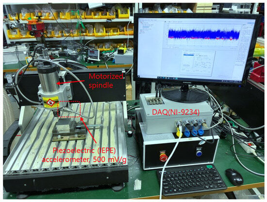
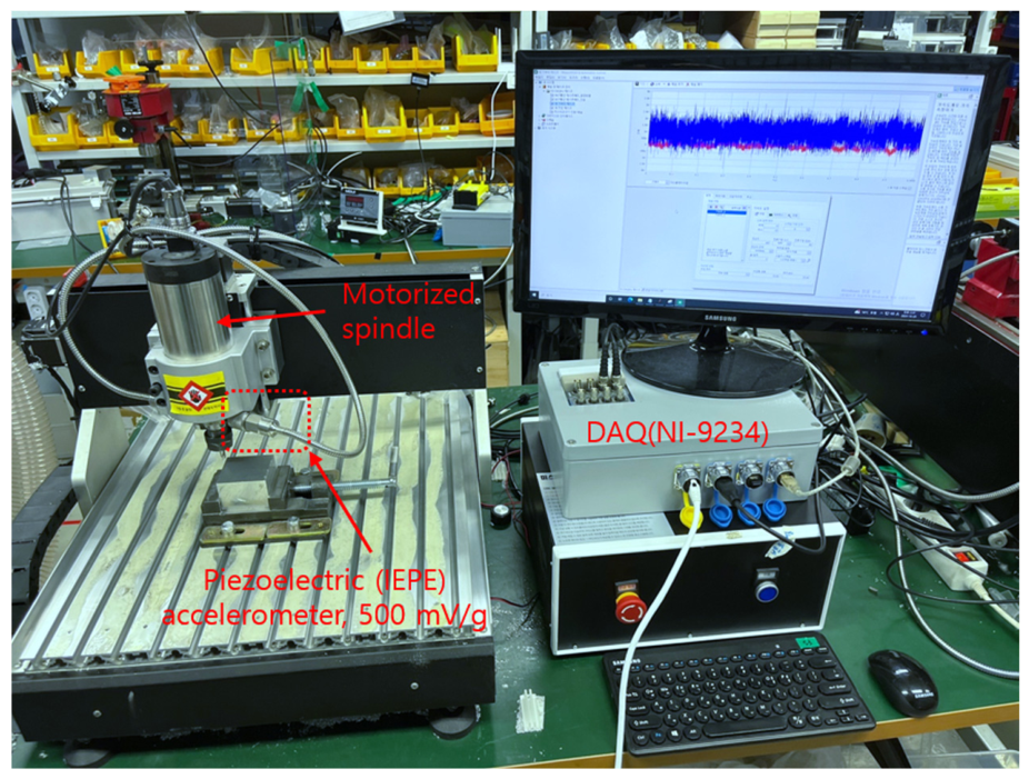
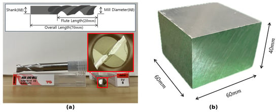
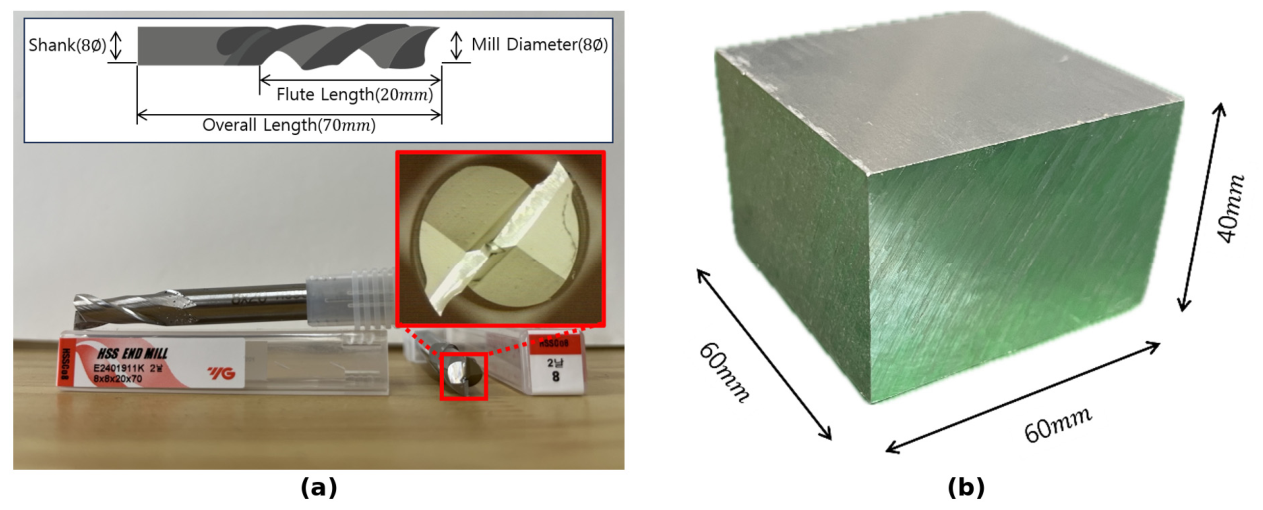
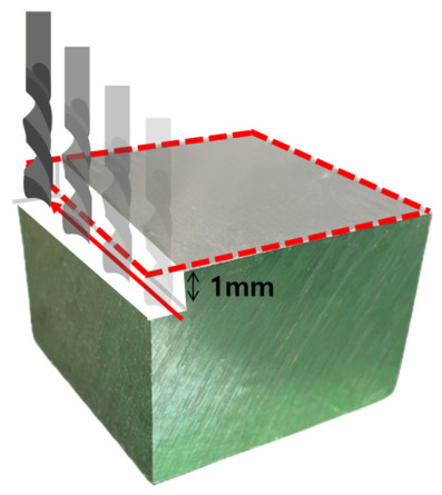
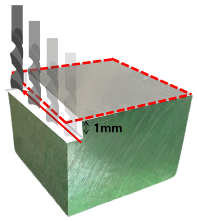
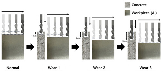
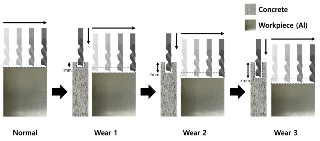
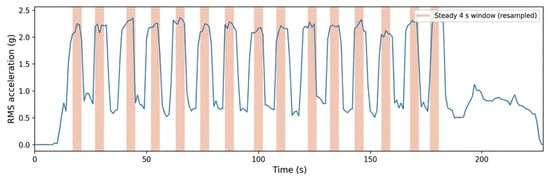
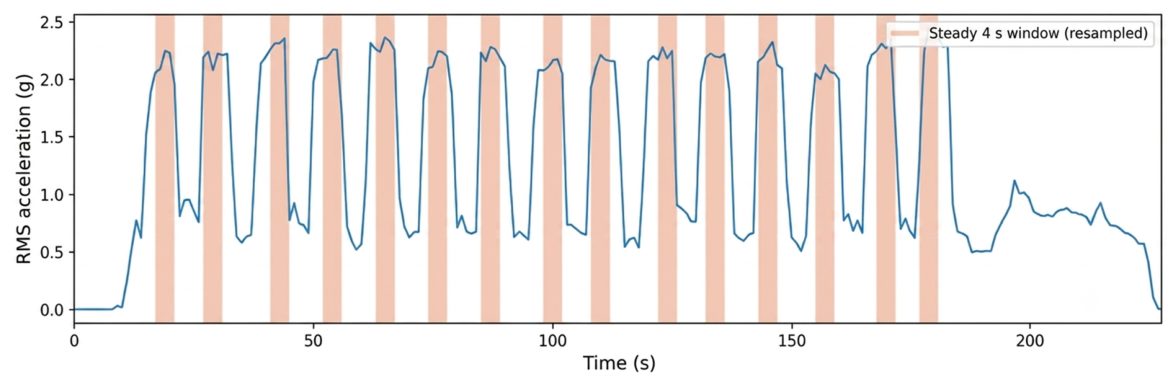
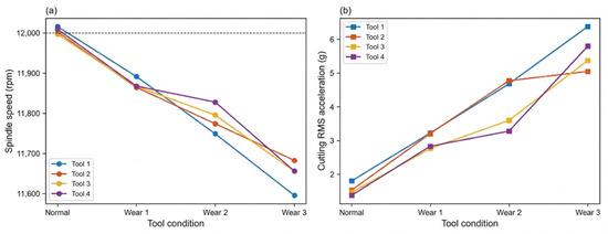
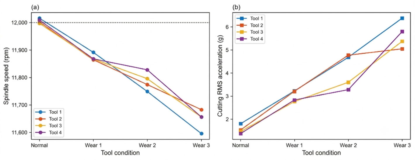
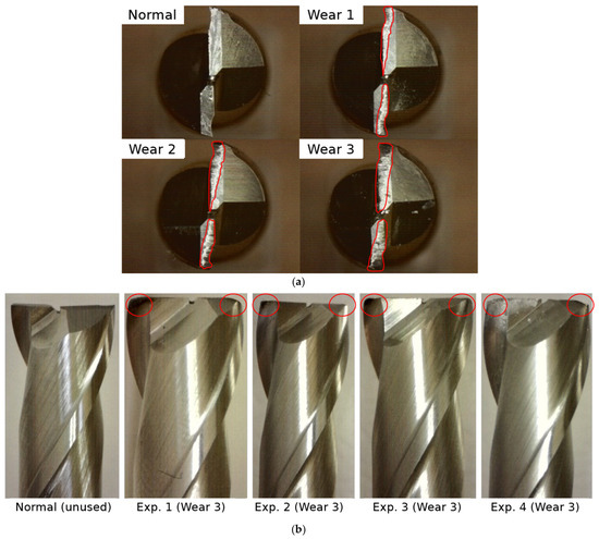
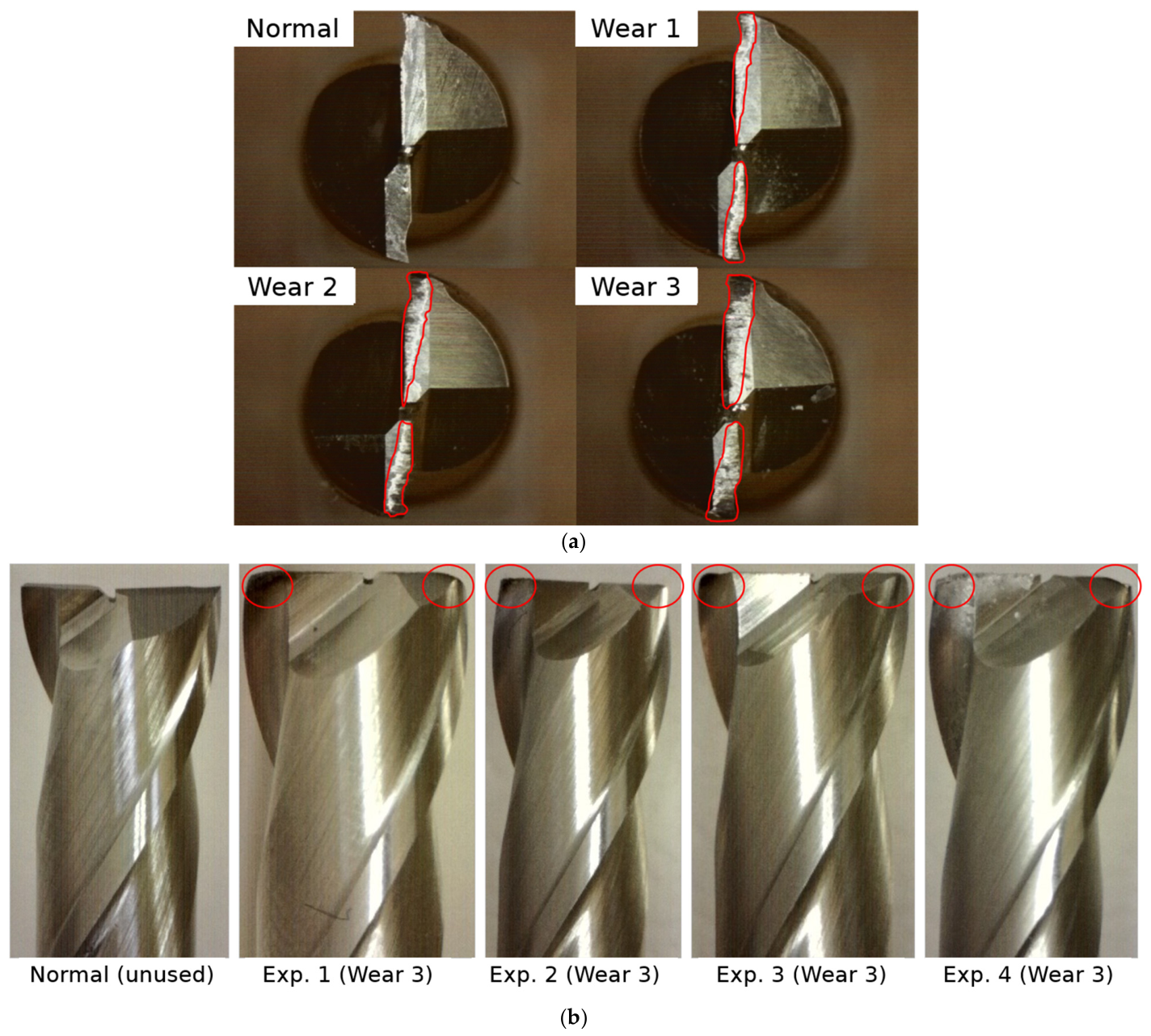
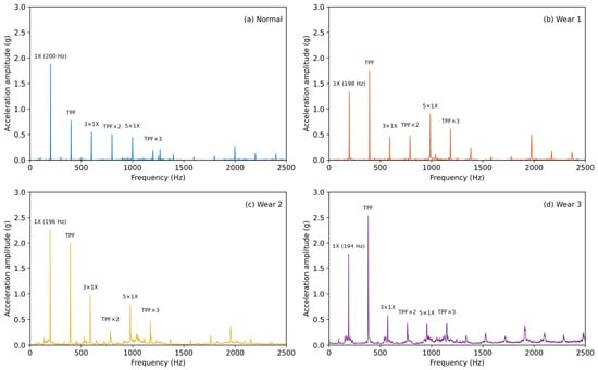
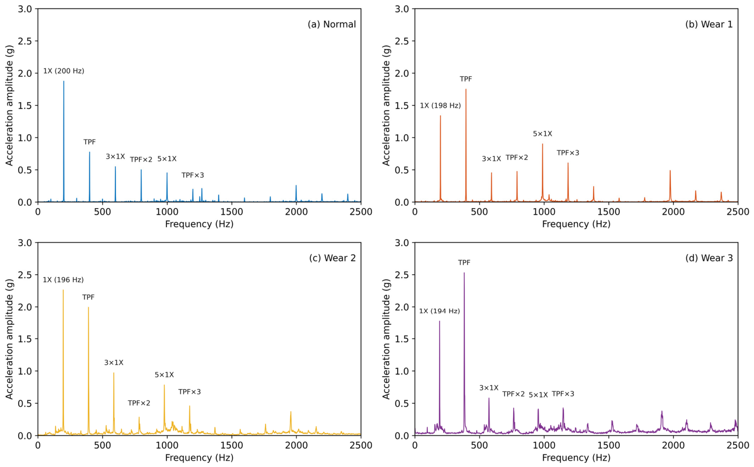
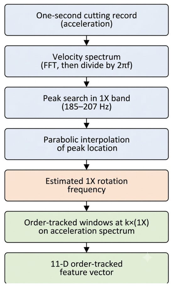
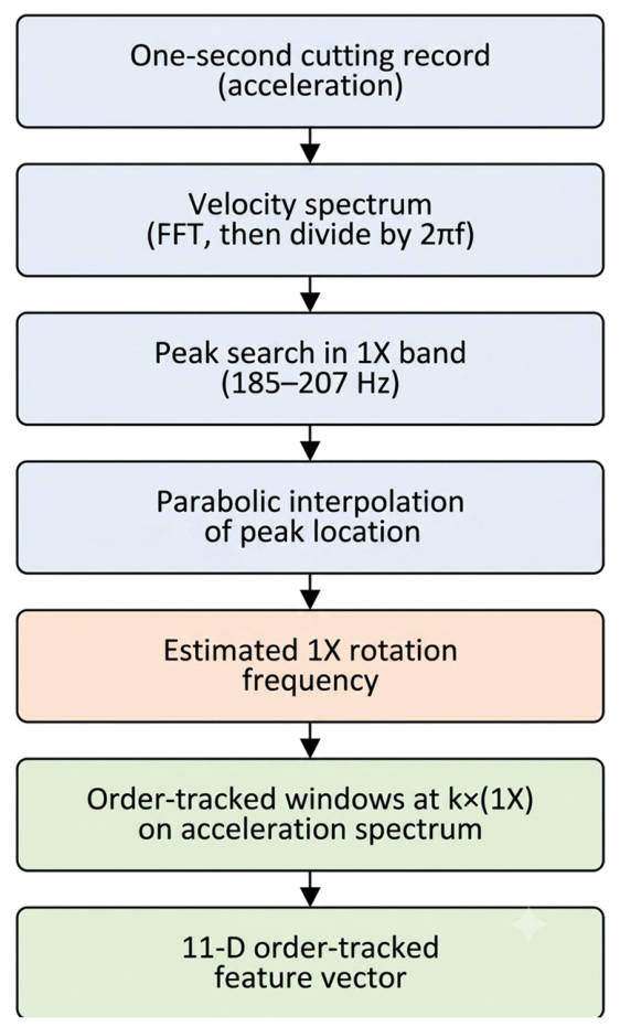
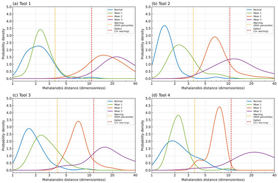
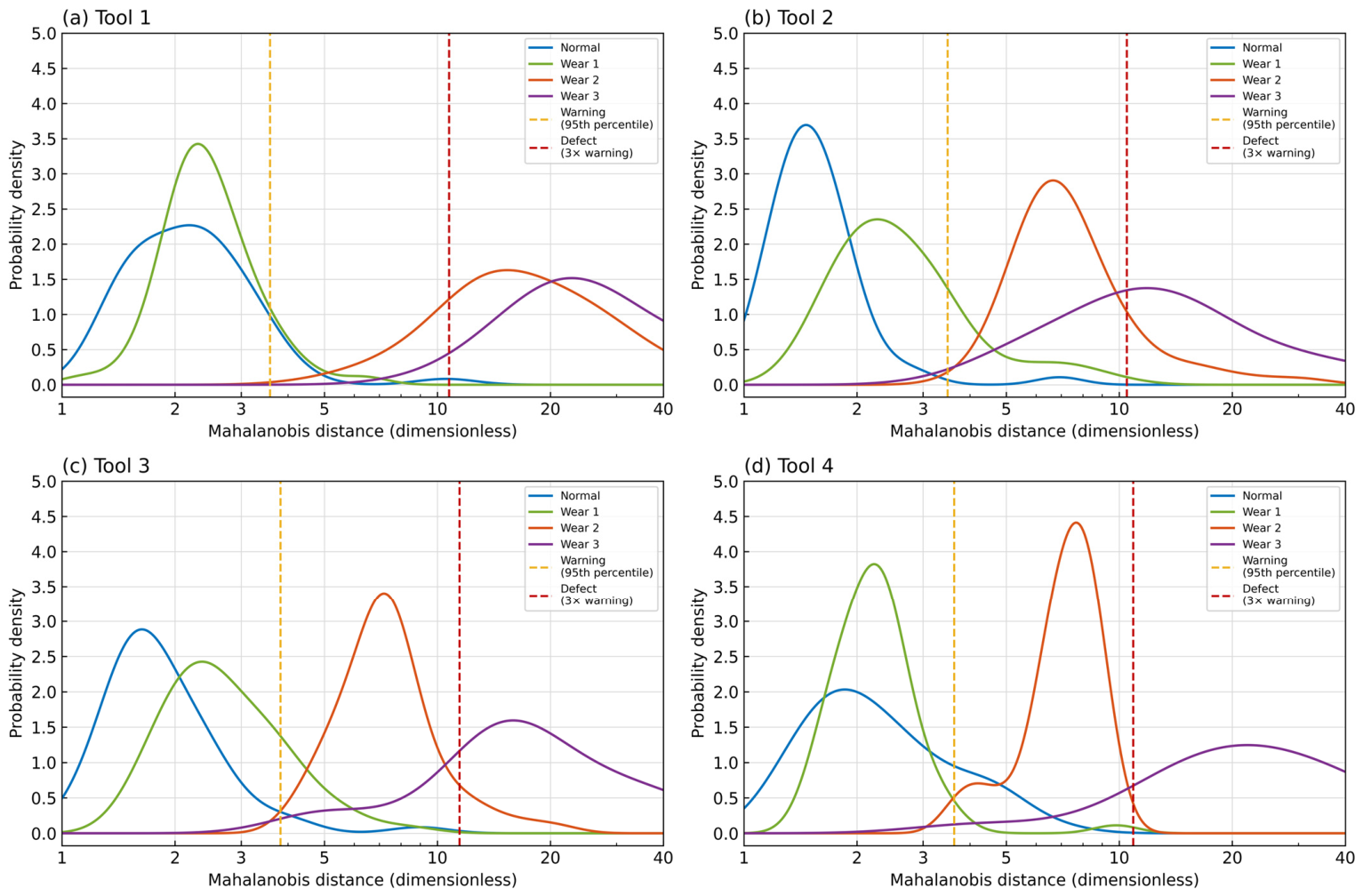
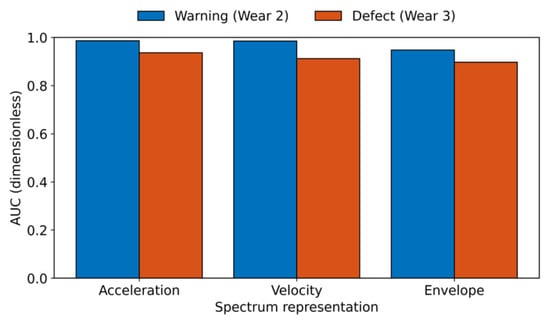
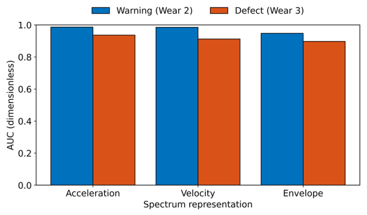
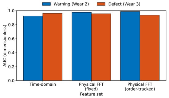
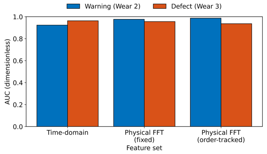
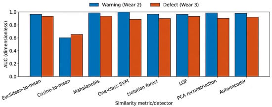
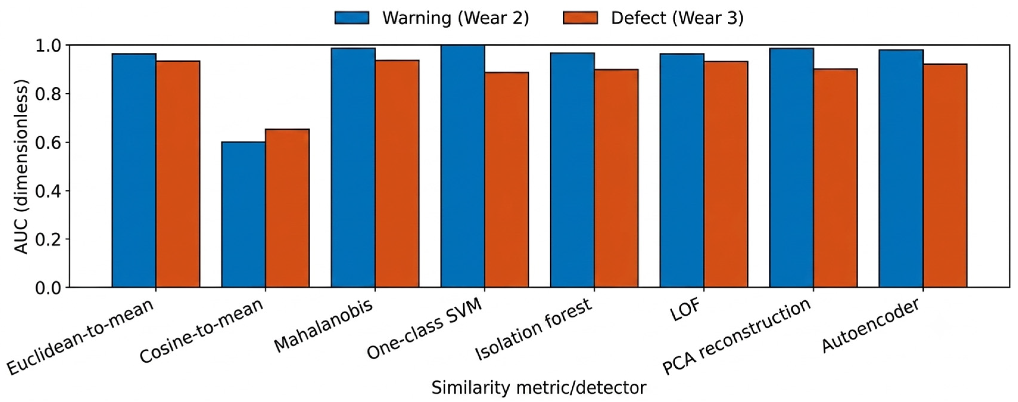
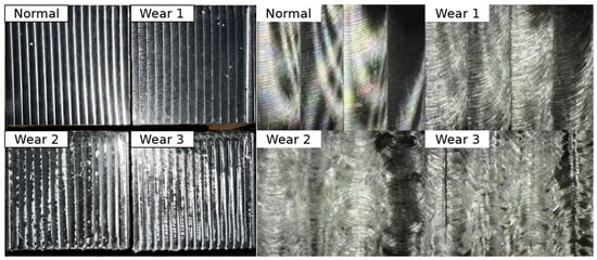
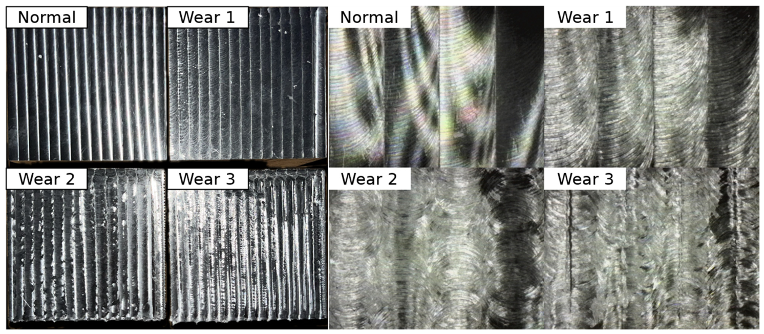
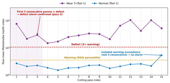
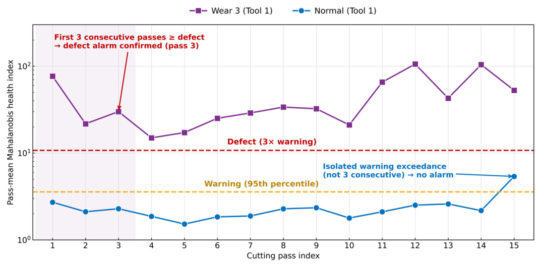
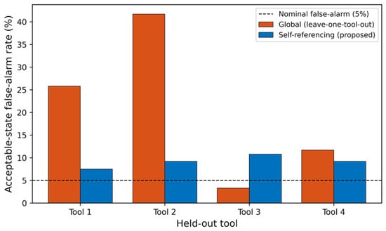
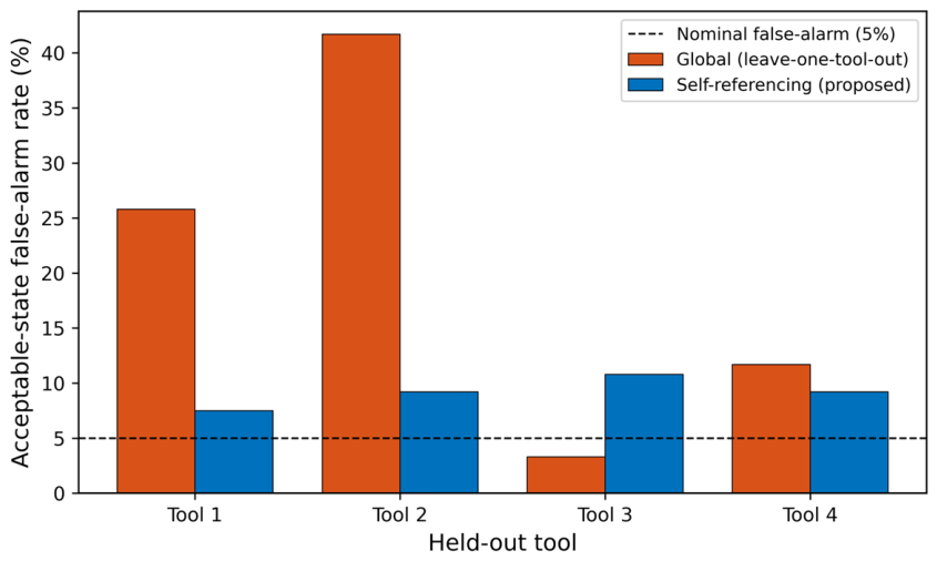
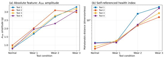
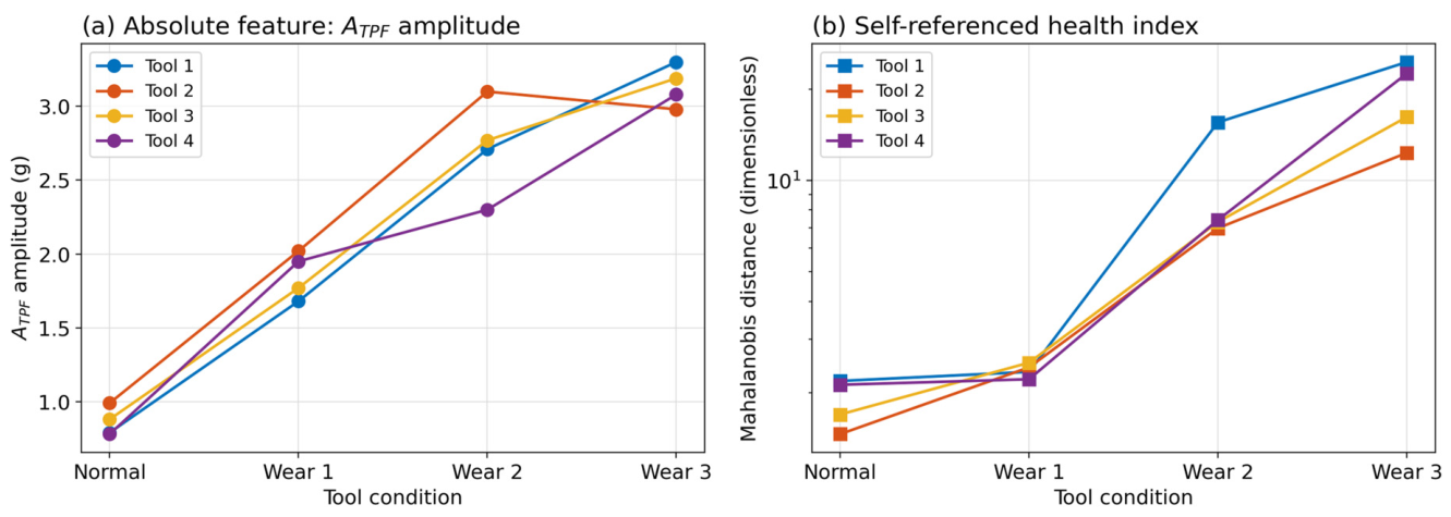
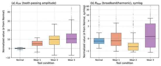
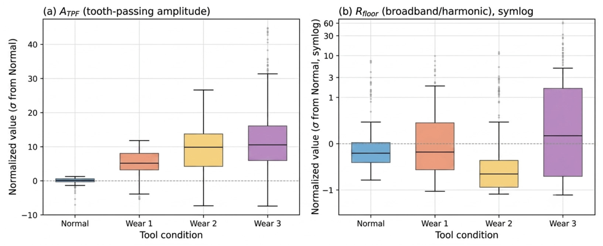

Disclaimer/Publisher’s Note: The statements, opinions and data contained in all publications are solely those of the individual author(s) and contributor(s) and not of MDPI and/or the editor(s). MDPI and/or the editor(s) disclaim responsibility for any injury to people or property resulting from any ideas, methods, instructions or products referred to in the content. |
© 2026 by the authors. Licensee MDPI, Basel, Switzerland. This article is an open access article distributed under the terms and conditions of the Creative Commons Attribution (CC BY) license.