


Abstract
To address the problems in hull form optimization where an increase in design variables requires approximation models to be rebuilt from scratch and historical CFD samples are insufficiently utilized, this paper proposes an incremental approximation model construction method. Based on the additive decomposition property of high-dimensional model representation, this method breaks through the rigid structure limitations of traditional approximation models. When dimension expansion occurs in the design space, it fully inherits existing low-order component models and historical sample point databases, requiring only local supplementary sampling and incremental construction for new variables and their strong coupling terms, thereby achieving adaptive cross-dimensional updates of the approximation model. The method is validated through numerical test functions and a container ship hull line resistance optimization case study. Results show that, compared with traditional full-dimensional approximation models, this method reduces full-space resampling overhead and maintains high prediction accuracy while reducing CFD sample requirements, providing an efficient modeling approach for ship hydrodynamic optimization in high-dimensional dynamic spaces.
1. Introduction
Driven by the demands of energy saving, emission reduction, and environmental regulations, efficient hull form optimization is crucial in modern ship design. Traditional hull form optimization typically relies on high-fidelity numerical simulation methods to evaluate the performance of different hull form design schemes. Although accurate in prediction, these methods are computationally expensive, presenting severe computational burdens when applied directly to large-scale design space searches. To address this, optimization methods based on approximation models are widely used in hull form design. By establishing a mapping relationship between design variables and hydrodynamic performance, these methods significantly reduce the number of CFD evaluations and improve optimization efficiency.
At present, approximation models such as Kriging [1,2,3], Radial Basis Functions (RBF) [4,5], Support Vector Regression (SVR) [6], and neural networks [7,8] have been widely applied in hull form optimization and resistance prediction. Combined with parametric geometry representation methods such as Free Form Deformation (FFD) [9] or NURBS surface control [10], approximation model-based optimization methods have achieved substantial progress in hull resistance prediction and line optimization. In practical applications, researchers have conducted extensive investigations to further enhance algorithm optimization efficiency for complex hull forms. For instance, regarding the integration of approximation models with intelligent optimization algorithms, Diez et al. [11] proposed a dynamic radial basis function (DRBF) model that significantly reduced the number of function evaluations required for high-dimensional engineering optimizations while ensuring the feasibility of the optimal solutions. Chang et al. [12] introduced a constraint-aware sampling framework integrated with SVM-based data mining, which substantially improved approximation model accuracy and optimization efficiency in the design of a 7500 DWT twin-tail bulk carrier. Huang et al. [13] combined an RBF interpolation model with an improved artificial bee colony (ABC) algorithm, successfully achieving resistance reduction for both the Series 60 and KCS hull forms. Additionally, Tran et al. [14,15] utilized Kriging approximation models to enable rapid hydrodynamic performance predictions for high-speed planing craft and wooden fishing vessels, respectively. Meanwhile, Feng et al. [16] and Mittendorf et al. [17] systematically constructed and benchmarked multi-objective approximation models for various container ships and catamarans, effectively boosting computational efficiency across multi-speed operating conditions; Zheng et al. [18] combined generative artificial intelligence with offline data-driven evolutionary algorithms to directly perform performance-driven search in a low-dimensional latent space by learning the implicit manifold of historical hull shape data, providing a new paradigm for hull form optimization that breaks the constraints of traditional parent-ship-based approaches. Kim [19] proposed an MLP-based hull form generation method with a geometric moment-based surrogate model, allowing each vertex of the hull mesh to move freely as a design variable and achieving efficient high-dimensional optimization on the KCS hull form.
However, in practical hull form optimization, the set of design variables does not always remain constant. There are two reasons for this. First, at the early stage of optimization, designers lack sufficient experience to determine the most appropriate parameter configuration and design space range at once, so it is usually necessary to add new geometric control parameters based on the existing ones and adjust them progressively during the iterative process. Second, the requirements of ship owners or users frequently change in engineering practice, so the optimization framework must be capable of adapting to new demands. When the number of design variables increases, traditional approximation models face a dilemma due to the lack of a spatially expandable structure: conducting full-dimensional resampling directly discards previously accumulated CFD simulation samples, resulting in a massive waste of computational resources; conversely, forcibly concatenating historical data using methods like baseline value padding easily disrupts the spatial distribution of sample points, leading to model prediction distortion.
To address the effective utilization of existing design data, researchers have recently proposed various data reuse and model updating methods. For example, Saida and Nishio [20] established a cross-domain indirect reuse mechanism using transfer learning and Gaussian process regression; Tfaily et al. [21] adopted a soft reuse architecture of “source-sample pre-training + target small-sample calibration” in aircraft design. In the field of naval architecture, Lee et al. [22] similarly incorporated transfer learning into their framework. By leveraging an existing baseline model of a 1000 TEU container ship, they achieved high-precision predictions of the wake field and viscous resistance across a series of 1800–3600 TEU container ships using only a small set of target samples; An et al. [23] integrated transfer learning with coarse and fine surrogate models for hull form optimization. This method achieved a 10.85% reduction in the total drag coefficient of KCS with a prediction error of only 2.93%, while reducing the required sample size by approximately half. Furthermore, to address the integration of multi-source and multi-fidelity data, Peherstorfer [24] systematically summarized the adaptation, fusion, and filtering paradigms in multi-fidelity modeling, providing a theoretical framework for the collaborative utilization of multi-source data; Liu [25] combined potential flow solvers with viscous flow solvers to construct a Co-Kriging model, achieving collaborative fusion of data with different physical fidelities. Bonfiglio et al. [26] and Renaud et al. [27] constructed multi-fidelity Gaussian process models targeting the seakeeping and multi-objective optimization of Small Waterplane Area Twin Hull (SWATH) vessels, effectively reducing multi-objective computational costs while maintaining optimization accuracy. However, these methods primarily focus on information transfer between data of different fidelities or within fixed design spaces, and the issue of model updating when design variable dimensions gradually increase still requires further investigation.
Inspired by the concept of Sobol variance decomposition [28], Rabitz and Alışınır (1999) proposed High-Dimensional Model Representation (HDMR) theory [29], which can decompose complex objective functions into a combination of low-order component functions. When combining the mathematical framework of HDMR with specific approximation models, its component-additive structural property exhibits natural scalability. Among these, the Kriging–HDMR method [30], which integrates Kriging models, effectively utilizes variable combinations of different orders to describe complex response relationships. Given the practical demand for gradually increasing design variables in hull form optimization, this paper introduces the Kriging–HDMR method into the hull form optimization process with dynamically increasing variables, proposing an incremental Kriging–HDMR modeling method. This method constructs a baseline Kriging–HDMR model in the initial variable space; when new design variables are introduced, low-order component models are built solely for the new variables and their necessary coupling terms, which are then combined with existing models for updating, thereby maximally preserving and reusing previously accumulated simulation samples.
The remainder of this paper is organized as follows: Section 2 introduces the theory of Sobol variance decomposition and High-Dimensional Model Representation (HDMR); Section 3 presents the detailed methodology of incremental Kriging–HDMR modeling; Section 4 validates the effectiveness of the method using high-dimensional nonlinear test functions; Section 5 applies the proposed method to a practical hull form resistance optimization problem and analyzes the results; and Section 6 concludes the paper.
2. Sobol Variance Decomposition and High-Dimensional Model Representation Theory
In approximation modeling of complex engineering systems, reducing model complexity while ensuring prediction accuracy represents a key approach to enhancing computational efficiency. Based on Sobol global sensitivity analysis [28], a multivariate objective function can be represented as a combination of individual variables and their interactions. According to Sobol decomposition theory, a black-box function defined on a multivariate domain can be expressed as:
In this expansion, is the functional mean, is the independent contribution of a single variable to the objective function, is the coupling effect between two variables, and higher-order terms are used to describe complex interaction effects among multiple variables.
For most engineering systems, constrained by physical laws, the system output is typically dominated by a few key variables and low-order variable interactions, whereas the contribution of higher-order interaction terms to the system response is relatively small [31]. Therefore, low-order truncated expansions are commonly adopted in engineering approximation modeling to strike a balance between accuracy and computational cost.
Based on the above concept, the High-Dimensional Model Representation (HDMR) method [29] expresses a complex objective function as a combination of multiple low-order component functions:
In this expansion, is the zeroth-order term, representing the true response at the reference point; is the first-order component function, representing the independent contribution of a single design variable to the objective function; and is the second-order component function, representing the contribution of the coupling effect between two variables to the objective function. The definitions of each low-order component function are as follows:
where denotes that all variables except the -th variable are fixed at the reference point ; similarly, the symbol indicates that only variables and are varied while all other dimensions remain fixed at the reference point .
Compared with directly constructing a full-dimensional approximation model, dimensional decomposition based on the HDMR structure decomposes the complex high-dimensional mapping into a sum of several independently constructed first- and second-order low-order component models. This decomposition approach for high-dimensional problems not only reduces the difficulty of model fitting, but also lays a foundation for directly reusing existing data when new variables are introduced later.
3. Incremental Modeling Method Based on HDMR Structure and Kriging Model
Traditional approximation models typically operate only under a fixed variable dimension. When additional control variables need to be added during the design process, the spatial structure of the model changes, making it impossible to directly reuse previously accumulated simulation data. This often requires fresh sampling and re-computation, leading to a waste of computational resources. To address the issue of legacy data becoming obsolete when design variables are added, this paper leverages the additive property of the HDMR structure to propose an incremental Kriging–HDMR modeling method.
The core idea of this method lies in the fact that when new variables are added, there is no need to discard the original model. Instead, the effect of the newly added variables is directly superimposed onto the existing model as an incremental term. This not only ensures the model’s predictive capability for the new variables, but also maximizes the reuse of existing CFD simulation data.
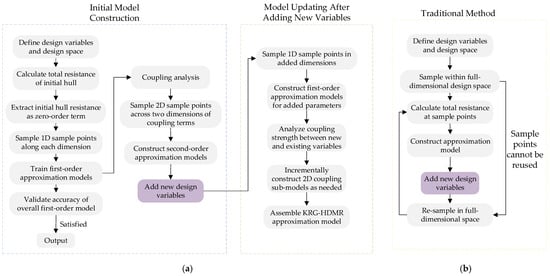
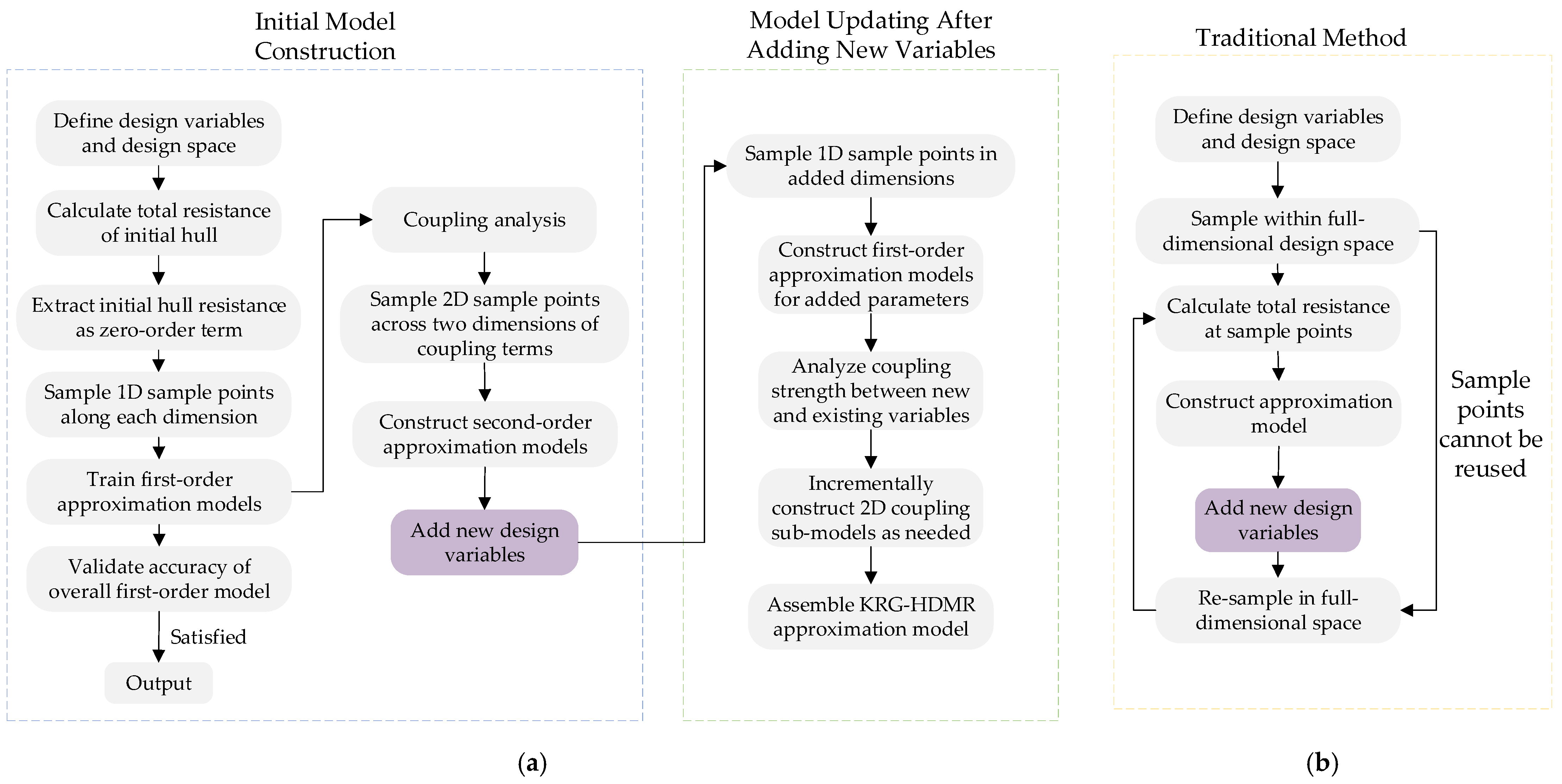
As shown in Figure 1, the construction process of this model consists of two main steps: initial model construction and model updating after introducing new variables:
Figure 1.
Comparison of workflows between incremental and traditional approximation model construction: (a) Incremental Kriging–HDMR approximation model construction and update workflow; (b) Traditional approximation model update workflow.
The specific steps of the aforementioned incremental modeling method are as follows:
Step 1: Taking the design parameters of the parent ship as the reference point, determine the design variable vector , and calculate the total resistance of the initial ship to obtain the constant term .
Step 2: Perform one-dimensional uniform sampling in each initial dimension . For the i-th design variable, uniformly select m sample points within its value range. The first-order incremental value at each sample point is calculated as:
where is the total resistance at the corresponding sample point, and is the total resistance of the initial hull form. Using the above one-dimensional sample data, the Kriging algorithm is employed to fit the first-order component model . All first-order component models are then accumulated to obtain the initial first-order additive model:
Step 3: Evaluate the second-order coupling intensity for candidate variable combinations . Fix the remaining design variables at the reference point, and vary only variables and to sample within the corresponding two-dimensional subspace to obtain . Use the existing first-order HDMR model to compute predicted values at these sample points, evaluate the coupling strength between variables based on the relative error between the true response values and first-order predictions, and calculate the relative error as follows:
If the error exceeds a preset threshold ε, a strong coupling effect is considered to exist. Uniform sampling is then performed in the corresponding two-dimensional subspace. For each two-dimensional sample point , the second-order incremental value is calculated as:
The Kriging algorithm is employed to fit the second-order component function . Finally, the initial baseline approximation model is assembled as:
where is the set of variable pairs with significant second-order coupling.
Step 4: When new design variables are added, keep the existing model and sample database unchanged, and perform supplementary one-dimensional sampling exclusively along the newly added dimensions to update the sample database.
Step 5: Construct individual first-order Kriging sub-models for each newly added variable , following the same sampling and modeling procedure as described in Step 2.
Step 6: For newly introduced variables and existing variable , follow the same procedure as in Step 3: for candidate variable pairs , fix all other variables at the reference point, vary only and to sample within the 2D subspace, and calculate the relative error between the true values and first-order predictions:
If , supplementary two-dimensional sampling is conducted to construct the corresponding second-order coupling term ; otherwise, this second-order term is neglected, following the same sampling and modeling procedure as described in Step 3.
Step 7: Superimpose the newly constructed low-order sub-models onto the original model to update and obtain the global approximation model in the expanded parameter space.
4. Numerical Example Validation
To evaluate the performance of the proposed incremental approximation model construction method across varying dimensions, degrees of nonlinearity, and variable coupling relationships, this section selects four representative high-dimensional mathematical benchmark functions for numerical simulation experiments. In the numerical experiments (F1–F4), the coupling screening threshold is set to ε = 0.05.
4.1. Test Functions
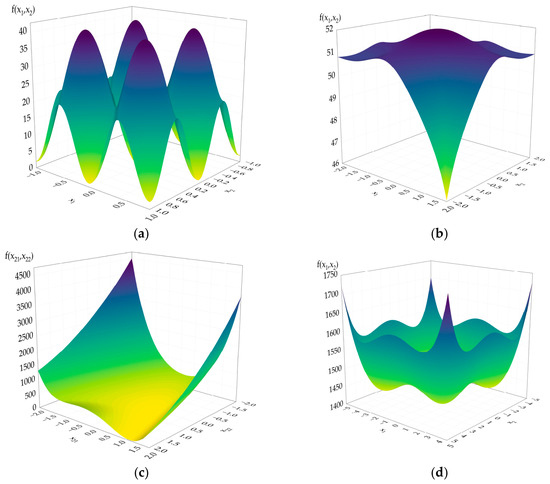
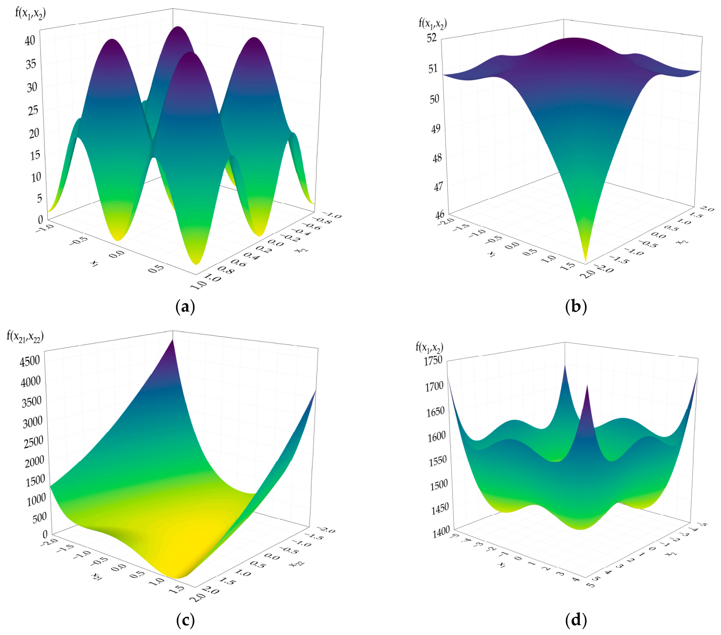
The mathematical formulas, dimensionality expansion schemes, and design spaces for each test case are listed in Table 1, and the corresponding 3D surface plots are shown in Figure 2.
Table 1.
Numerical experiments.
Figure 2.
3D surface plots of test functions. (a) 3D surface plot of function F1; (b) 3D surface plot of function F2; (c) 3D surface plot of function F3; (d) 3D surface plot of function F4. Color gradient represents the value, yellow (lowest) to purple (highest).
4.2. Error Metrics
In this study, Maximum Relative Error (maxRE), Relative Average Absolute Error (RAAE), and Normalized Root Mean Square Error (nRMSE) are employed as error metrics. The calculation formulas for each metric are as follows:
where is the true response value of the -th sample in the test set; is the corresponding predicted value from the approximation model; is the total number of test sample points (an independent Latin Hypercube Sampling test set with is uniformly adopted for all numerical examples in this paper); and , and are the standard deviation, maximum value, and minimum value of the true responses in the test set, respectively.
4.3. Results and Discussion
To demonstrate the sample reuse advantages and fitting accuracy of the proposed method as the number of variables increases, cross-dimensional prediction comparative experiments are conducted between the proposed incremental modeling method, the traditional standard Kriging model, and neural network models. Table 2 details the parameter configurations of the Kriging and neural network surrogate models used in the cross-dimensional comparative study. The convergence of the neural network is monitored via the default early-stopping mechanism implemented in MATLAB R2021a’s feedforwardnet. Training terminates when either (1) the gradient of the performance function falls below 1 × 10⁻⁷, or (2) the validation mean squared error (MSE) fails to decrease for six consecutive epochs . In all experiments of this study, the training converged before reaching the maximum epoch limit (1000), with stable validation performance and no significant overfitting.
Table 2.
Key parameter configurations for Kriging and neural network surrogate models.
During the testing process, at the initial dimensionality , all models (Kriging, NN, and Kriging–HDMR) independently generated their training samples according to their respective sampling strategies. Specifically, Kriging and NN employed full-dimensional uniform sampling, while Kriging–HDMR constructed its component models based on one-dimensional and two-dimensional low-dimensional uniform sampling. To ensure the fairness of the comparison, the total number of training samples for each model was kept at a comparable order of magnitude (Kriging and NN used integer multiples of samples, with their total counts slightly higher than that of Kriging–HDMR). The test set consisted of 100 sample points drawn by Latin hypercube sampling over the full space of the initial dimensionality , and the same test set was shared by all three approximation models for evaluation. This setup provides a relatively fair basis for comparing the global approximation capabilities of the different models.
When design variables expand to a higher dimension , the proposed method retains all sample points from the stage, collecting only a small number of additional samples for the newly added dimensions and their necessary coupling terms. To ensure a fair comparison under equivalent computational resources, the traditional standard Kriging and neural network methods also adopt a data reuse strategy commonly used in engineering when constructing the -dimensional model, so as to simulate the practical engineering constraint where high sample acquisition costs necessitate the retention of existing samples. The baseline models pad historical samples from the stage with zeros along the new dimensions and combine them with the newly added samples. A global approximation model for the dimension is then jointly trained using this hybrid sample set of equivalent size. It should be noted that such a “zero-padding” operation is not the optimal modeling approach for conventional methods, but merely a simplified proxy to maintain comparable sample sizes under the incremental scenario. Therefore, the comparison in this stage is intended to evaluate the adaptability of different methods under conditions of gradual dimensional expansion and limited data availability, rather than serving as an alternative to the rigorous full-dimensional accuracy comparison conducted at the initial dimensionality. Similar to the initial dimensionality, the test set consists of 100 sample points drawn by Latin hypercube sampling over the full space of the expanded dimensionality , and the same test set is shared by all three approximation models for evaluation. The quantitative comparison results are presented in Table 3.
Table 3.
Comparison of error metrics and sampling requirements of different approximation models under increasing dimensionality (for the Kriging–HDMR model, values in parentheses are formatted as “total (first-order + second-order)”).
As shown by the experimental comparison in Table 3, when the design space undergoes dimensional expansion, the proposed method requires only a small number of incremental samples to complete the model update, demonstrating a significant advantage in data reuse. For example, in function F1, after the variables expand from 10 to 12 dimensions, Kriging–HDMR inherits the approximation model structure from the 10-dimensional space and only requires 20 additional samples in the 12-dimensional space, along with the local approximation structures corresponding to the two new variables. This enables the approximation model to maintain the same level of accuracy in the 12-dimensional space as in the 10-dimensional space, with maxRE slightly changing from 4.46% to 4.59% (a variation of only 2.91%). In contrast, under the same addition of 20 sample points, Kriging’s maxRE increased from 21.94 to 48.53 (a 121.19% increase), and its nRMSE shifted from 0.2336 to 0.2805 (a 20.08% change); for the NN model, maxRE rose from 28.38 to 102.40 (a 260.82% surge), while nRMSE went from 0.4094 to 0.4942 (a 20.71% increase). This demonstrates that, with the same sample size, Kriging–HDMR achieves an accuracy an order of magnitude higher than both standard Kriging and NN models.
For function F2, after the variables expand from 20 to 22 dimensions, Kriging–HDMR requires selecting only 42 additional samples along with the local approximation model structures corresponding to these two newly added variables. The variations in its maxRE and RAAE remain small, and its nRMSE changes from 0.0555 to 0.0489—a variation of merely 11.89%—thereby maintaining high accuracy. In contrast, when 60 additional sample points are selected, Kriging’s maxRE metric increases from 20.29 to 28.75 (a 41.70% change), while NN’s maxRE rises from 26.47 to 31.69 (a 19.72% variation). This demonstrates that, despite using 10% fewer sample points, Kriging–HDMR delivers an accuracy an order of magnitude higher than both standard Kriging and NN models.
For function F3, after the variables expand from 20 to 22 dimensions, Kriging–HDMR requires selecting only 119 additional samples. Its maxRE increases from 10.10 to 13.13, RAAE slightly decreases from 0.1947 to 0.1638, and nRMSE changes from 0.0457 to 0.0378—a variation of merely 17.29%—thereby maintaining high accuracy. In contrast, when 120 additional samples are selected, Kriging’s maxRE soars from 96.12 to 150.61 (a 56.64% change), while NN’s maxRE rises from 203.06 to 225.15 (a 10.88% variation). This demonstrates that, despite using fewer sample points, Kriging–HDMR delivers accuracy that is approximately one order of magnitude higher than both standard Kriging and NN models.
For function F4, after the variables expand from 30 to 32 dimensions, Kriging–HDMR requires selecting only 28 additional samples along with the local approximation model structures corresponding to these two newly added variables. Its maxRE changes from 3.90 to 4.03 (a variation of only 3.33%), RAAE moves from 0.1088 to 0.1160 (a change of merely 6.62%), and nRMSE shifts from 0.0274 to 0.0300 (varying by just 9.49%). In contrast, when 60 additional sample points are selected, Kriging’s maxRE metric changes from 52.14 to 55.15 (a 5.77% variation) and its RAAE moves from 0.8417 to 0.9049 (a 7.51% change); for the NN model, RAAE shifts from 1.2010 to 0.9571 (a 20.31% variation) and nRMSE decreases from 0.3098 to 0.2508 (a 19.04% change). This demonstrates that, despite requiring 20% fewer sample points, Kriging–HDMR achieves an accuracy an order of magnitude higher than both standard Kriging and NN models.
Kriging–HDMR consistently outperforms standard Kriging and neural networks in terms of prediction error, whether on additive functions, nonseparable functions [32], or problems involving high-order interaction terms. Its superiority becomes even more pronounced in high-dimensional settings, thereby validating the effectiveness of the proposed method in complex interaction scenarios [33,34]. In terms of predictive accuracy, conventional full-dimensional approximation models—even when forcibly reusing historical data—struggle to overcome the curse of dimensionality under limited new samples, leading to severe accuracy deterioration. In contrast, by leveraging the additive structure of low-order decomposition, the proposed method consistently maintains prediction errors at a low level across test cases of varying dimensions and complexities. The results demonstrate that the proposed method achieves efficient cross-dimensional updating of approximation models at a low sample cost, while maintaining high modeling accuracy and stability.
5. Hull Form Optimization Test Case
5.1. Optimization Model and Strategy
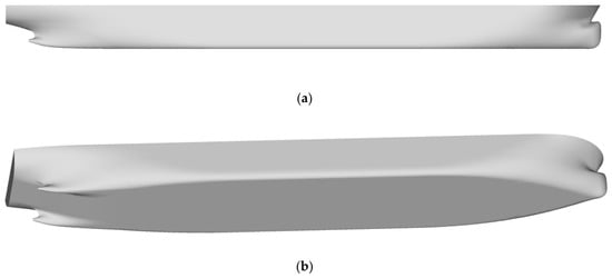
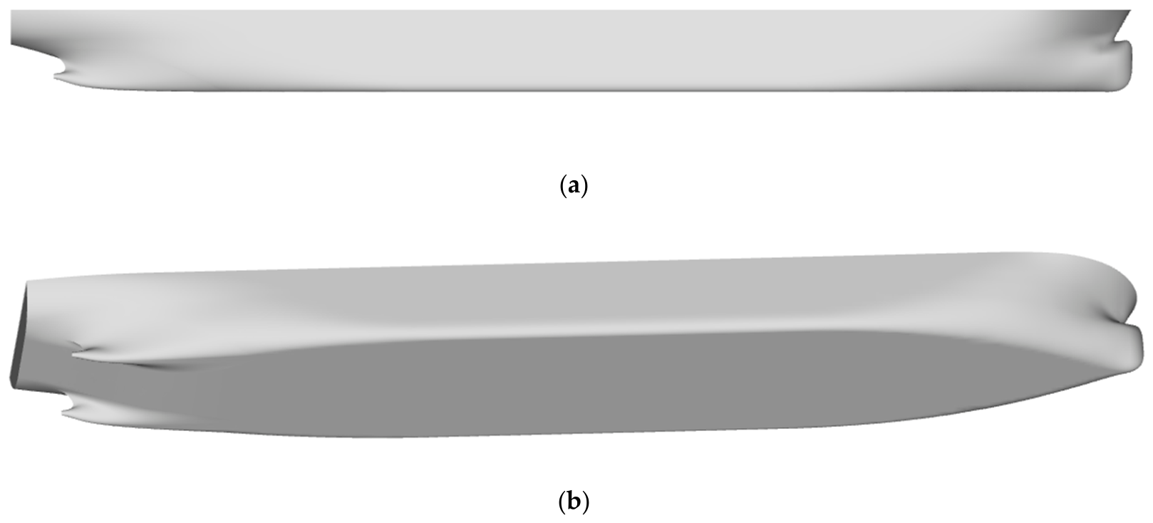
This section takes the hull line optimization of an 800 TEU container ship as an example to verify the performance of the incremental Kriging–HDMR method under practical engineering scenarios. The optimization design aims to minimize the total resistance of the vessel under the operating condition at Froude number . The three-dimensional geometric model of the ship hull is shown in Figure 3, and the principal dimensions are listed in Table 4.
Figure 3.
3D schematic diagram of the 800 TEU container ship: (a) Side view of an 800 TEU container ship; (b) Bottom view schematic of an 800 TEU container ship.
Table 4.
Principal dimensions of the initial 800 TEU container ship.
Displacement volume constraint: ; this constraint is used to ensure that the displacement volume of the optimized hull is not lower than the initial design value.
Longitudinal center of buoyancy constraint: ; this constraint aims to control the variation range of the longitudinal center of buoyancy of the optimized hull form within 1% of the initial hull form.
Using parametric modeling technology, in the initial modeling stage, based on engineering experience in parametric modeling, we focused on selecting geometric control parameters that significantly affect total resistance, and 14 design variables (numbered 1 to 14) are first selected to form the initial design space. The maximum feasible domain of each variable is determined by the geometric fairness constraints of the parametric model. On this basis, the variation ranges are further narrowed down to a reasonable interval by combining the initial hull parameters and engineering experience. In the subsequent refined optimization stage, to further explore the resistance reduction potential of the stern hull lines, two local control variables (numbered 15 and 16) are introduced to expand the design space to 16 dimensions. The specific design parameters are shown in Table 5.
Table 5.
Design parameters of the 800 TEU container ship.
Table 6 provides a summary of the CFD methodology parameters used in the present resistance simulations.
Table 6.
CFD methodology parameters for the resistance simulation.
To verify the accuracy of the CFD results, a grid independence verification was conducted in this study. Three sets of grids (coarse, medium, and fine) were established for convergence analysis, and the total resistance results are presented in Table 7. The formula for calculating the grid convergence ratio is as follows:
Table 7.
Grid independence verification and convergence ratio.
The calculated convergence ratio is , which satisfies , indicating that the numerical results have achieved monotonic convergence [35]. As the grid is progressively refined, the computed total resistance exhibits only small fluctuations near the fine-grid solution, suggesting that the results have stabilised and meet the requirements for engineering accuracy. Considering the balance between computational precision and resource consumption, the medium grid was adopted for all subsequent simulations.
For the training set, the sample points in the hull-form optimization case are generated using a one-dimensional uniform sampling strategy. Specifically, each design variable is independently sampled along its one-dimensional range. In the 14-dimensional and 16-dimensional design spaces, the numbers of first-order training samples are 126 (14 × 9) and 144 (16 × 9), respectively. It should be noted that only the first-order Kriging–HDMR approximation model is constructed in this case, and no second-order component samples are collected. The reason is that, as shown in Table 8, the first-order model achieves a maximum relative error of 2.49% in the 14-dimensional space and 3.73% in the 16-dimensional space, both of which fall within the acceptable engineering accuracy range. Therefore, to avoid the substantial increase in computational cost associated with second-order sampling while maintaining prediction reliability, no further second-order sample points are collected in this study.
Table 8.
Prediction errors of the Kriging–HDMR model under different dimensions.
To verify the prediction accuracy of the model, 20 independent test sample points were extracted in the 14-dimensional and 16-dimensional design spaces, respectively, using the Sobol sequence. By leveraging the additivity of low-order component functions, the incremental Kriging–HDMR method effectively reduces the reliance on high-dimensional sample sizes, demonstrating excellent prediction accuracy with small sample sizes in high-dimensional spaces as well as high data reuse efficiency. The prediction errors in each design space are shown in Table 8. With a cumulative total of only 144 CFD samples consumed, its maximum relative errors in the 14-dimensional and 16-dimensional spaces were stably controlled within 2.49% and 3.73%, respectively.
5.2. Global Optimization and Results Comparison
Based on the constructed approximation model in the 16-dimensional expanded design space, a global optimization search for the total resistance of the hull form was performed using the NSGA algorithm. The population size was set to 50, and the number of generations was set to 48. Due to the stochastic nature of the optimization algorithm, three optimization runs were conducted under the same settings in this study. Table 9 presents the specific numerical comparison of the 16 optimization variables for the three optimized hull forms. To verify the actual resistance reduction effect of the optimization schemes, CFD numerical simulations were performed on the resulting optimized hull forms, and the comparison results between prediction and validation are shown in Table 10. Experimental results show that the optimized hull forms derived based on the incremental Kriging–HDMR model all demonstrate good resistance reduction performance and high prediction accuracy. Among them, Optimized Hull 3 achieves the most significant resistance reduction, with the total resistance reduced from 13.26 N of the initial hull form to 12.55 N, representing a resistance reduction rate of 5.35%. Furthermore, the relative error between the predicted value of the approximation model and the CFD simulation value is only 2.07%. These results demonstrate that the incremental approximation model constructed in this study maintains high prediction accuracy even after expanding the design space dimensions, and the resistance reduction performance of the resulting optimized hull forms is effectively validated by CFD simulations.
Table 9.
Numerical comparison of optimization variables before and after optimization.
Table 10.
Comparison of resistance and prediction accuracy of optimized hull forms in the 16-dimensional expanded design space.
Due to the stochastic nature of the NSGA algorithm, three independent optimization runs were conducted under identical settings to assess the robustness of the results. As summarized in Table 10, the three optimized hull forms exhibit consistent resistance reduction performance, with total resistance decreasing by 4.68%, 4.30%, and 5.35%, respectively, relative to the initial hull. The relative errors between the approximation model predictions and the CFD validation results are 0.23%, 3.62%, and 2.07%, respectively, showing no systematic bias. The good consistency across the three independent runs and the stable prediction–validation agreement demonstrate that the optimization results are robust and that the approximation model maintains reliable predictive capability throughout the expanded design space.
Table 11 presents a comparison of the hydrostatic parameters between each optimized hull form and the initial hull form at full scale. The results indicate that the displacement volumes of all three optimized hulls show an extremely slight increase, with variations consistently within 0.08%—specifically, increases of 0.08% for Optimized Hull 1, 0.01% for Optimized Hull 2, and 0.001% for Optimized Hull 3. Regarding wetted surface area, Optimized Hull 1 increased by 0.76%, Optimized Hull 2 decreased by 0.04%, and Optimized Hull 3 increased by 0.31%. The shifts in the longitudinal center of buoyancy for all hull forms are minimal, ranging between –0.02 m and +0.03 m, with relative changes not exceeding 0.05%.
Table 11.
Comparison of hydrostatic parameters before and after optimization (coordinate origin: bottom of transom stern, positive X forward).
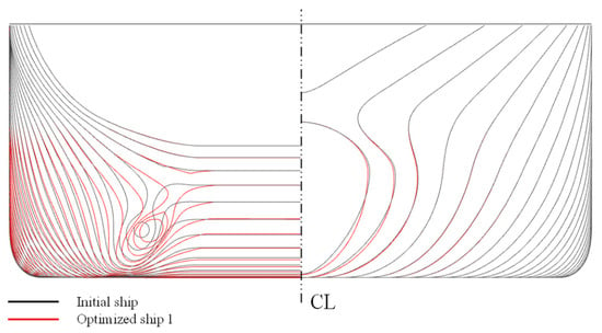
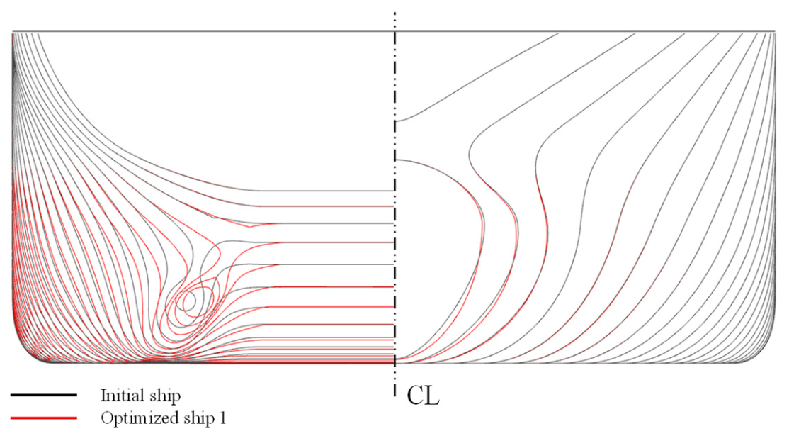
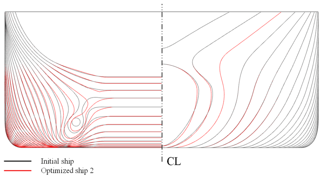
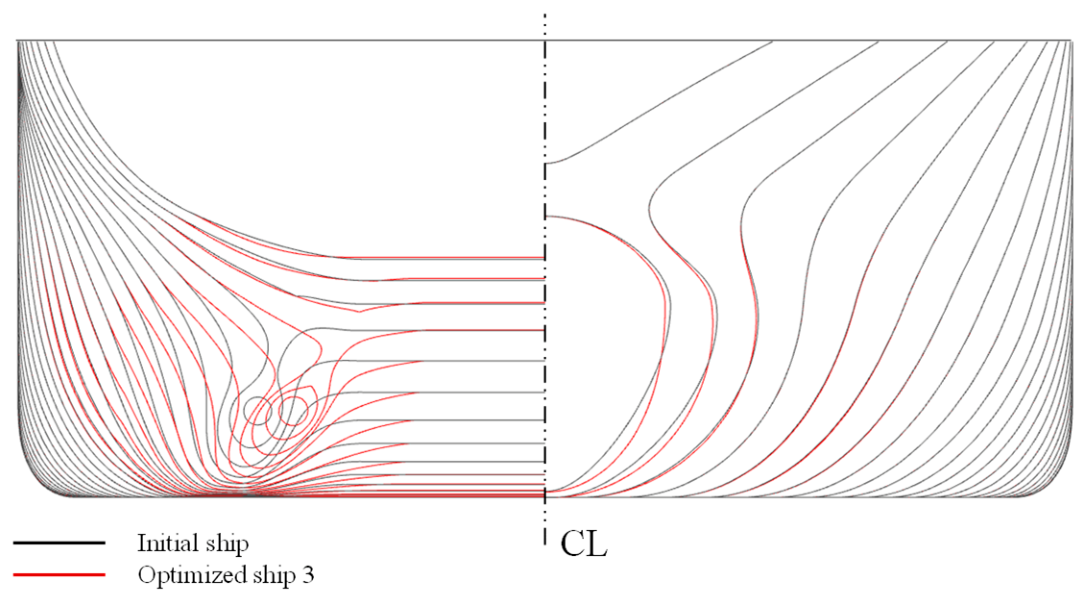
From the body plan comparisons in Figure 4, Figure 5 and Figure 6, it can be seen that in the 16-dimensional expanded design space, the hull lines at both the bow and stern of the optimized hulls underwent changes, with the variations at the stern being noticeably more pronounced. Specifically, the stern lines of Optimized Hull 1 contract inward in the region of the twin shaft lines, whereas the bow lines show only a slight outward expansion in localized areas below the design draft, with most section lines largely coinciding with those of the initial hull. Optimized Hull 2 exhibits a smaller degree of inward contraction in the twin-shaft region, with a slight offset in the middle and lower portions of the bow, presenting a relatively smooth overall variation. For Optimized Hull 3, the scope of adjustment in the twin-shaft region at the stern is broader, showing a more pronounced inward contraction of the transverse section lines; below the waterline, the bow contracts slightly while remaining closely aligned with the section lines of the initial hull.
Figure 4.
Comparison of section lines between initial hull and Optimized Hull 1.
Figure 5.
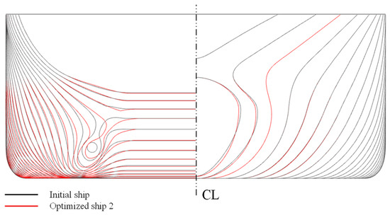
Comparison of section lines between initial hull and Optimized Hull 2.
Figure 6.
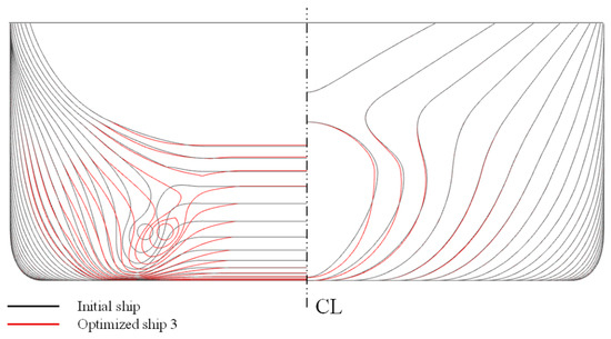
Comparison of section lines between initial hull and Optimized Hull 3.
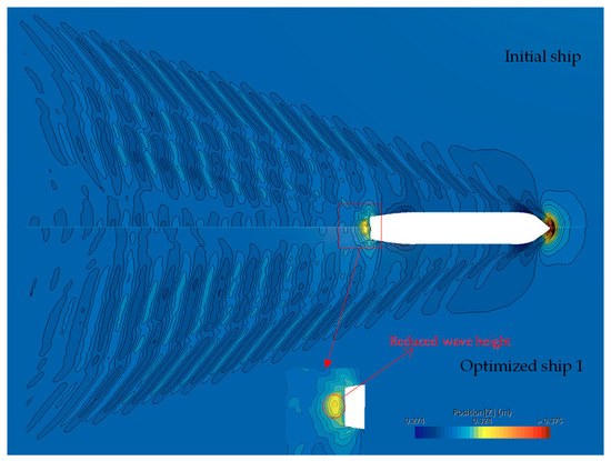
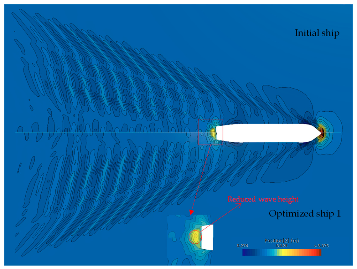
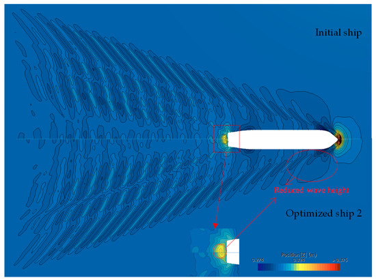
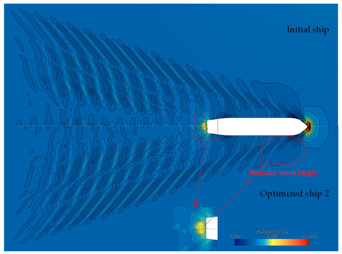
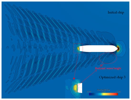
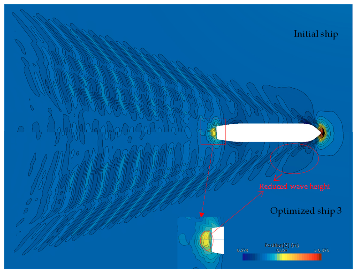
From the wave pattern comparisons between the initial hull and each optimized hull form in Figure 7, Figure 8 and Figure 9, it can be observed that the wave-making amplitudes of the optimized hulls are reduced, and the extent of far-field wave disturbance is noticeably narrowed. Looking at the enlarged close-up views of the stern, the initial hull generates a pronounced localized high wave-height region near the stern. In contrast, after optimization, the stern wave heights for all three optimized hull forms are reduced to varying degrees, with the area of the high wave-height region shrinking significantly. Among them, Optimized Hull 3 demonstrates the most pronounced suppression effect on stern waves, where the high wave crest region is substantially flattened, and the divergent wave disturbance on both sides is minimal. This indicates that the optimized hull lines improve the flow field at the stern, thereby reducing energy loss during the wave-making process. This observation is consistent with the resistance calculation results in Table 11, indicating that the improvement in stern wave-making is one of the primary reasons for the reduction in total resistance.
Figure 7.
Comparison of wave patterns between initial hull and Optimized Hull 1 (the specific locations with improved wave patterns (reduced wave height) are clearly marked with red boxes, circles, and arrows.).
Figure 8.
Comparison of wave patterns between initial hull and Optimized Hull 2 (the specific locations with improved wave patterns (reduced wave height) are clearly marked with red boxes, circles, and arrows.).
Figure 9.
Comparison of wave patterns between initial hull and Optimized Hull 3 (the specific locations with improved wave patterns (reduced wave height) are clearly marked with red boxes, circles, and arrows.).
6. Conclusions
To address the high construction costs and the need for re-sampling in traditional approximation models as the number of design variables increases, this paper proposes an incremental Kriging–HDMR approximation model construction method. Validated through numerical test cases and applied to container ship hull line optimization, the following conclusions are drawn:
- (1)
- Achieving lossless data reuse: When facing the expansion of design space dimensions, the proposed method can fully inherit the previously constructed low-order component models and historical samples. Model updates can be completed by adding only a minimal number of samples for the new variables, thereby avoiding the wastage of computational resources and sample distortion caused by starting from scratch or forced model concatenation in traditional approaches.
- (2)
- Ensuring modeling stability under high-dimensional, small-sample conditions: Based on the low-order additive decomposition of HDMR, the proposed method effectively mitigates the “curse of dimensionality” and fitting distortion to which traditional full-dimensional approximation models are susceptible under high-dimensional, small-sample conditions. It consistently maintains low prediction errors across various test dimensions.
- (3)
- Demonstrating practical engineering value: In the 16-dimensional hull line optimization of an 800 TEU container ship, a high-precision approximation model was successfully constructed using only 144 CFD sample points. The optimal hull form obtained through optimization achieved a 5.35% reduction in total resistance, with a model prediction error of only 2.07%, validating the feasibility and efficiency of the proposed method in hull form optimization.
However, it should be noted that, due to the lack of publicly available towing tank test data for this 800 TEU container ship, the resistance of the initial hull could not be directly validated against experimental data, and the numerical uncertainty has not been quantified. Although the present study has demonstrated the convergence of the numerical method through grid independence verification, the physical significance of the reported 5.35% resistance reduction still requires further confirmation through model experiments or more accurate validation approaches.
Author Contributions
Conceptualization, H.C. and Q.Z.; methodology, Q.Z.; software, Q.Z.; validation, H.C., Q.Z. and P.L.; formal analysis, Q.Z. and P.L.; investigation, Q.Z.; resources, H.C.; data curation, Q.Z.; writing—original draft preparation, Q.Z.; writing—review and editing, H.C.; visualization, Q.Z.; supervision, H.C.; project administration, H.C.; funding acquisition, H.C. All authors have read and agreed to the published version of the manuscript.
Funding
This research was funded by the National Natural Science Foundation of China, grant number 52471339.
Data Availability Statement
The original contributions presented in this study are included in the article. Further inquiries can be directed to the corresponding author.
Conflicts of Interest
The authors declare no conflicts of interest.
References
- Liu, Z.; Zhao, W.; Wan, D. Resistance and wake distortion optimization of JBC considering ship-propeller interaction. Ocean Eng. 2022, 244, 110376. [Google Scholar] [CrossRef] [Scilit]
- Liu, X.; Ji, X.; Wang, L.; Rong, Z.; Sun, X.; Yuan, L. A novel expected improvement-sequentially constrained Monte Carlo method for hull form optimization. Ocean Eng. 2026, 346, 123905. [Google Scholar] [CrossRef] [Scilit]
- Xin, L.; Liu, P.; Wang, S.; Yan, J.; Bai, C. Hierarchical multi-objective hull optimization for a cross-domain unmanned surface and glide vehicle based on Voronoï-EHVI adaptive sampling. Ocean Eng. 2026, 343, 123397. [Google Scholar] [CrossRef] [Scilit]
- Liu, X.; Zhao, W.; Wan, D. Hull form optimization based on calm-water wave drag with or without generating bulbous bow. Appl. Ocean Res. 2021, 116, 102861. [Google Scholar] [CrossRef] [Scilit]
- Kim, H.; Yang, C. A new surface modification approach for CFD-based hull form optimization. J. Hydrodyn. 2010, 22, 520–525. [Google Scholar] [CrossRef] [Scilit]
- Feng, Y.; Chen, Z.; Dai, Y.; Wang, F.; Cai, J.; Shen, Z. Multidisciplinary optimization of an offshore aquaculture vessel hull form based on the support vector regression surrogate model. Ocean Eng. 2018, 166, 145–158. [Google Scholar] [CrossRef] [Scilit]
- Liu, Z.; Wan, D.; Zhang, X.; Chen, J.; Wang, S.; Wang, Y. Design space nonlinear dimensionality reduction based on deep neural networks in ship hull form optimization. Ocean Eng. 2026, 348, 124112. [Google Scholar] [CrossRef] [Scilit]
- Wei, Y.; Pan, G.; Paladaechanan, P.; Wan, D. A novel hull form optimization framework based on multi-fidelity deep neural network. J. Hydrodyn. 2025, 37, 149–159. [Google Scholar] [CrossRef] [Scilit]
- Campana, E.F.; Peri, D.; Tahara, Y.; Stern, F. Shape optimization in ship hydrodynamics using computational fluid dynamics. Comput. Methods Appl. Mech. Eng. 2006, 196, 634–651. [Google Scholar] [CrossRef] [Scilit]
- Qi, X.; Miao, A.; Wan, D. A Nurbs-Based Hull Surface Modification Method for Hydrodynamic Optimization. In Proceedings of the Thirteenth ISOPE Pacific/Asia Offshore Mechanics Symposium, Jeju, Republic of Korea, 14–17 October 2018. [Google Scholar]
- Diez, M.; Volpi, S.; Serani, A.; Stern, F.; Campana, E.F. Simulation-Based Design Optimization by Sequential Multi-Criterion Adaptive Sampling and Dynamic Radial Basis Functions. In Advances in Evolutionary and Deterministic Methods for Design, Optimization and Control in Engineering and Sciences; Computational Methods in Applied Sciences; Springer: Cham, Switzerland, 2019; Volume 48, pp. 213–228. [Google Scholar]
- Chang, H.; Hou, W.; Liu, Z.; Feng, B.; Zheng, Q. Enhancing surrogate model accuracy in ship design optimization through intelligent constraint-aware sample selection. Eng. Appl. Artif. Intell. 2026, 163, 112716. [Google Scholar] [CrossRef] [Scilit]
- Huang, F.; Wang, L.; Yang, C. A new improved artificial bee colony algorithm for ship hull form optimization. Eng. Optim. 2016, 48, 672–686. [Google Scholar] [CrossRef] [Scilit]
- Tran, T.G.; Nguyen, H.V.; Van Huynh, Q. A Method for Optimizing the Hull Form of Fishing Vessels. J. Ship Res. 2023, 67, 72–91. [Google Scholar] [CrossRef] [Scilit]
- Tran, T.G.; Van Huynh, Q.; Kim, H.C. Optimization strategy for planing hull design. Int. J. Nav. Archit. Ocean Eng. 2022, 14, 100471. [Google Scholar] [CrossRef] [Scilit]
- Feng, Y.; Moctar, O.E.; Schellin, T.E. Parametric Hull Form Optimization of Containerships for Minimum Resistance in Calm Water and in Waves. J. Mar. Sci. Appl. 2021, 20, 670–693. [Google Scholar] [CrossRef] [Scilit]
- Mittendorf, M.; Papanikolaou, A.D. Hydrodynamic hull form optimization of fast catamarans using surrogate models. Ship Technol. Res. 2021, 68, 14–26. [Google Scholar] [CrossRef] [Scilit]
- Zheng, L.; Wang, H.; Chen, S. The generative marine hull form optimization based on offline data-driven evolutionary algorithm. Ocean Eng. 2026, 358, 125935. [Google Scholar] [CrossRef] [Scilit]
- Kim, J.; Roh, M.; Yeo, I. An MLP (Multi-Layer Perceptron)-based method for optimizing multiple hull forms at once using surrogate modeling with geometric moments. Ocean Eng. 2025, 339, 122121. [Google Scholar] [CrossRef] [Scilit]
- Saida, T.; Nishio, M. Transfer learning Gaussian process regression surrogate model with explainability for structural reliability analysis under variation in uncertainties. Comput. Struct. 2023, 281, 107014. [Google Scholar] [CrossRef] [Scilit]
- Tfaily, A.; Bartoli, N.; Diouane, Y.; Kokkolaras, M. Transfer learning in surrogate modeling with emphasis on aircraft design. Struct. Multidiscip. Optim. 2026, 69, 41. [Google Scholar] [CrossRef] [Scilit]
- Lee, M.; Lee, I. A machine-learning based prediction of wake distribution for feeder-class container ships with flow control fins. Ocean Eng. 2025, 340, 122372. [Google Scholar] [CrossRef] [Scilit]
- An, C.; Mao, L. A Transfer Learning Based Dual-Surrogate-Assisted Hull Form Optimization Method. Jisuanji Gongcheng/Comput. Eng. 2025, 51, 317–327. [Google Scholar]
- Peherstorfer, B.; Willcox, K.; Gunzburger, M. Survey of Multifidelity Methods in Uncertainty Propagation, Inference, and Optimization. SIAM Rev. 2018, 60, 550–591. [Google Scholar] [CrossRef] [Scilit]
- Liu, X.; Zhao, W.; Wan, D. Multi-fidelity Co-Kriging surrogate model for ship hull form optimization. Ocean Eng. 2022, 243, 110239. [Google Scholar] [CrossRef] [Scilit]
- Bonfiglio, L.; Perdikaris, P.; Vernengo, G.; de Medeiros, J.S.; Karniadakis, G. Improving SWATH Seakeeping Performance using Multi-Fidelity Gaussian Process and Bayesian Optimization. J. Ship Res. 2018, 62, 223–240. [Google Scholar] [CrossRef] [Scilit]
- Renaud, P.; Sacher, M.; Scolan, Y. Multi-objective hull form optimization of a SWATH configuration using surrogate models. Ocean Eng. 2022, 256, 111209. [Google Scholar] [CrossRef] [Scilit]
- Sobol, I.M. Global sensitivity indices for nonlinear mathematical models and their Monte Carlo estimates. Math. Comput. Simul. 2001, 55, 271–280. [Google Scholar] [CrossRef] [Scilit]
- Rabitz, H.; Aliş, Ö.F. General foundations of high-dimensional model representations. J. Math. Chem. 1999, 25, 197–233. [Google Scholar] [CrossRef] [Scilit]
- Tang, L.; Li, G.; Wang, H. Kriging-HDMR metamodeling technique for nonlinear problems. Lixue Xuebao/Chin. J. Theor. Appl. Mech. 2011, 43, 780–784. [Google Scholar]
- Li, G.; Wang, S.; Rabitz, H. Practical Approaches to Construct RS-HDMR Component Functions. J. Phys. Chem. A Mol. Spectrosc. Kinet. Environ. Gen. Theory 2002, 106, 8721–8733. [Google Scholar] [CrossRef] [Scilit]
- Czworkowski, C.L.; Sheppard, J.W. Using Variable Interaction Graphs to Improve Particle Swarm Optimization. In GECCO ’25 Companion: Proceedings of the Genetic and Evolutionary Computation Conference Companion, Malaga, Spain, 14–18 July 2025; Association for Computing Machinery: New York, NY, USA, 2025; pp. 479–482. [Google Scholar]
- Alimhillaj, P.; Minisci, E.; Dalla Vedova, M.D.L.; Ferro, C.G.; Maggiore, P. Interpretable surrogate modelling for multirotor design exploration: Combining HDMR and Kolmogorov-Arnold decomposition. In Proceedings of the MDPI 1st International Online Conference on Aerospace, Online, 16–17 April 2026. [Google Scholar]
- Zhong, L.; Yang, Y.; Zha, Z.; Shu, L.; Jiang, P.; Zhou, Q.; Wang, C. A space mapping-based high-dimensional model representation for multi-fidelity surrogate modelling. Eng. Optim. 2026, 58, 1652–1678. [Google Scholar] [CrossRef] [Scilit]
- Farkas, A.; Degiuli, N.; Martic, I. Assessment of hydrodynamic characteristics of a full-scale ship at different draughts. Ocean Eng. 2018, 156, 135–152. [Google Scholar] [CrossRef] [Scilit]

Disclaimer/Publisher’s Note: The statements, opinions and data contained in all publications are solely those of the individual author(s) and contributor(s) and not of MDPI and/or the editor(s). MDPI and/or the editor(s) disclaim responsibility for any injury to people or property resulting from any ideas, methods, instructions or products referred to in the content. |
© 2026 by the authors. Licensee MDPI, Basel, Switzerland. This article is an open access article distributed under the terms and conditions of the Creative Commons Attribution (CC BY) license.