Modular Performance Testing and Comparative Evaluation Method for Wind Turbine Retrofit Schemes

Abstract

To overcome the limitations of existing evaluation methods and performance testing for wind power generation systems, this study proposes a modular framework for performance testing and comparative assessment. Methodologically, the approach establishes a baseline configuration for simulation and provides optional interfaces for experimental, hardware-in-the-loop, or bench testing under identical boundary conditions. By employing a unified metric system, the proposed method enables a comprehensive evaluation of annual energy production (AEP) gains, power curve deviations, damage equivalent loads (DEL) when cycle-resolved load histories are available, fatigue- and peak load proxy variations, efficiency fluctuations, temperature rise margins, and reliability proxy indicators. A demonstrative case study is conducted using illustrative numerical data parameterized for a generic 2.5 MW-class doubly fed wind turbine to compare three retrofit schemes: blade replacement, gearbox optimization (S2), and a pitch system upgrade. When annual energy production (AEP) is utilized as the sole metric, the blade replacement scheme yields a 3.32% increase. However, it concurrently increases the fatigue load and peak load proxies by 6.11% and 3.72%, respectively. Conversely, a comprehensive assessment incorporating load, temperature rise, vibration, and reliability identifies the gearbox optimization (S2 scheme) as the highest-ranked option under the current weighting configuration, with a reproducible overall score of 0.65. The weight sensitivity analysis further shows that the preferred scheme can change when engineering priorities change. Ultimately, this work demonstrates the proposed method’s capability to highlight the discrepancy between single-metric and holistic performance optimization, providing standardized support for scheme selection, project acceptance, and the evaluation of wind turbine retrofit schemes.

1. Introduction

Driven by the dual-carbon goals of carbon peaking and carbon neutrality, renewable energy assets—such as wind turbines and photovoltaic systems—are transitioning into a phase of large-scale operation and maintenance. Consequently, the industry paradigm is shifting from rapid capacity expansion to operational optimization and efficiency enhancement. This transition is particularly critical for legacy units with extended service histories. Subjected to prolonged complex loading, environmental weathering, component wear, and obsolete control strategies, these aging systems frequently suffer from degraded power performance, amplified structural loads, escalating component failure rates, and surging maintenance costs. Compared with new installations, technical retrofits of legacy equipment offer lower capital intensity, shorter implementation cycles, and more predictable economic returns. Consequently, measures such as blade replacement, gearbox optimization, pitch system upgrades, and control parameter reconfiguration have emerged as primary engineering strategies to enhance the operational performance of renewable energy plants [1,2,3]. However, the ultimate viability of a retrofit scheme extends beyond single-metric gains, such as increased energy production. It necessitates a comprehensive evaluation of post-retrofit performance dynamics, encompassing revenue generation, structural loads, operational efficiency, and system reliability.

In practice, evaluating the efficacy of retrofits for renewable energy equipment typically relies on two primary approaches: empirical analysis utilizing field trials, SCADA data, and power curve comparisons; and offline simulations employing multibody dynamics, aeroelastic, or control system models. While the empirical approach accurately captures real-world performance and is supported by mature standardization frameworks for power testing, load measurement, and field acceptance [4,5], it presents inherent limitations. Specifically, relying solely on field data makes it challenging to compare different retrofit schemes under identical boundary conditions. This difficulty stems from the stochastic nature of wind and the inability to maintain consistent environmental and operational variables—such as air density, turbulence intensity, yaw errors, and curtailment strategies—across distinct testing periods. Particularly in wind turbine applications, even when adhering to standard power curve testing methods, variations in operational filtering criteria, data-cleaning protocols, and statistical windows across sample batches can yield biased evaluation outcomes [5,6]. Conversely, simulation-based approaches offer high testing efficiency, excellent repeatability, and suitability for batch screening, facilitating the rapid identification of scheme viability during early design stages. However, without rigorous validation against field, hardware-in-the-loop (HIL), or bench test data, these models may exhibit systematic discrepancies between their parameter settings and the actual equipment state [6,7,8]. Consequently, neither empirical field data nor simulation alone can provide sufficient support for robust engineering decision-making in renewable energy retrofit projects.

Furthermore, alongside the widespread deployment of renewable energy systems, the engineering criteria for retrofit evaluation have shifted from simply maximizing energy yield to balancing economic benefits with rigorous risk mitigation. Existing literature indicates that wind turbine power capture capabilities, mechanical load levels, control response dynamics, and fault evolution processes are strongly coupled. Consequently, a given retrofit strategy may inadvertently induce elevated fatigue and extreme loads, accelerate actuator wear, or degrade vibration and thermal characteristics, thereby compromising equipment lifespan and operational reliability [9,10,11,12]. For instance, while aerodynamic blade optimization increases energy capture in low-to-medium wind regimes, it can concurrently amplify blade-root bending moments and drivetrain torsional loads. Similarly, although gearbox optimization enhances transmission efficiency, its impact on thermal and vibration profiles necessitates further empirical verification. While pitch system upgrades can effectively mitigate peak loads, suboptimal tuning of control parameters may compromise the dynamic stability of the turbine under complex wind conditions [13,14]. Consequently, the rigorous evaluation of renewable energy retrofit schemes must no longer be confined to single-metric comparisons. Rather, a multidimensional framework encompassing economic revenue, structural loads, operational efficiency, and system reliability must be established to yield statistically robust and engineering-interpretable conclusions under a standardized baseline.

Concurrently, recent advancements in digital twins, model calibration, uncertainty assessment, and verification and validation methodologies have provided useful technical support for evaluating complex equipment performance [15,16,17,18]. A robust retrofit evaluation system must satisfy four fundamental criteria: (1) consistent test boundaries, ensuring that different schemes are compared under identical operational conditions, control criteria, and evaluation periods; (2) model credibility, necessitating that simulations are parametrically calibrated and cross-validated using experimental, bench, or hardware-in-the-loop (HIL) data; (3) standardized metrics, guaranteeing that evaluation variables—such as revenue, loads, efficiency, and reliability—share consistent data sources, calculation bases, and interpretation logic; and (4) result traceability, establishing explicit linkages among operational condition packages, model versions, datasets, algorithms, and output results to satisfy engineering acceptance and auditing protocols [18,19]. Despite these prerequisites, the current literature and engineering practices still lack an auditable pipeline that combines parallel multi-scheme comparison, optional numerical–physical validation, explicit data provenance, non-compensatory feasibility screening, and transparent ranking for wind turbine retrofit assessment.

The novelty of the proposed method lies in the integration of four mechanisms rather than in any single established technique: (1) a frozen baseline/plug-in configuration rule that isolates the effect of each retrofit; (2) a uniquely identified operating condition package that enforces identical boundary conditions; (3) a consistency and provenance layer that distinguishes numerical reference data from optional physical validation data; and (4) a two-stage decision rule that applies non-compensatory feasibility constraints before normalized weighted ranking and weight sensitivity analysis.

To address these evaluation requirements, this study proposes a modular performance testing and comparative assessment framework tailored for wind energy retrofits. Building upon a baseline model configuration, candidate schemes are formulated by integrating plug-and-play retrofit modules. Unified operational condition packages are then synthesized by merging standard operating conditions with a comprehensive test case library. The framework supports simulations and, where available, experimental, hardware-in-the-loop, or bench data under strictly identical boundary conditions; the present case activates only the numerical branch. A consistency verification and parameter calibration loop is retained as a general framework capability. Employing a standardized metric system, the approach evaluates annual energy production (AEP) gains, power curve deviations, damage equivalent load (DEL) when cycle-resolved load histories are available, response-level fatigue- and peak load proxies in the present case, efficiency, temperature, vibration, and reliability proxy indicators.

2. System Architecture and Evaluation Framework

2.1. System Architecture and Design Concept

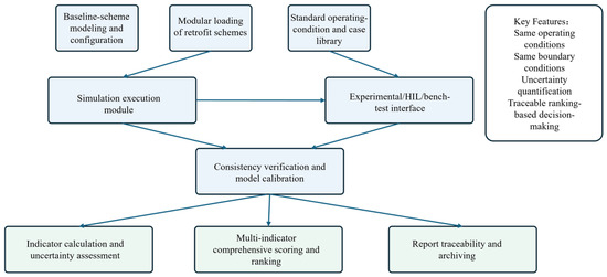
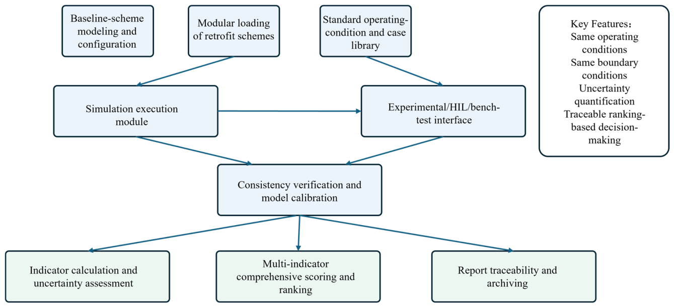
As illustrated in Figure 1, the proposed modular performance testing and comparative evaluation framework comprises eight core modules: (1) baseline modeling and configuration; (2) plug-and-play retrofit integration; (3) operating conditions and test case library; (4) simulation execution and result management; (5) experimental/hardware-in-the-loop (HIL)/bench–test interfacing; (6) consistency verification and model calibration; (7) metric calculation and uncertainty assessment; and (8) comparative ranking and report traceability. Interconnected via standardized data interfaces, these modules facilitate both rapid batch evaluations in the simulation environment and critical operational validation on physical equipment. Ultimately, this architecture establishes an end-to-end closed-loop pipeline encompassing modeling, testing, validation, evaluation, and traceability [7,8].

Figure 1. Overall architecture of the modular performance testing and comparative evaluation system.

Specifically, the architectural design prioritizes the following principles. First, the structural parameters, control logic, and interfaces of unaltered components are anchored via baseline modeling, ensuring consistent boundary conditions for multi-scheme comparisons. Second, targeted subsystems—such as blades, gearboxes, and pitch systems—are either virtually replaced or parametrically updated via a plug-and-play mechanism, facilitating the rapid interchange of retrofit schemes within a unified platform. Third, environmental and operational variables (e.g., wind speed bins, turbulence classes, yaw errors, and curtailment constraints) are synthesized into standardized operational packages to eliminate comparison biases. Finally, simulation outcomes can be compared with experimental, HIL, or bench data when such physical data are available, thereby providing an optional physical validation path for industrial applications [9,10,11]. The baseline is frozen only during the controlled comparison stage so that changes can be attributed to the active retrofit module; after a candidate passes the feasibility screen, a subsequent co-optimization stage may retune structural or control parameters subject to the same safety constraints.

The standardized operating condition and test case library serve as a crucial foundation for unbiased comparative assessments. In engineering practice, this library is structured across key dimensions, including wind speed bins, turbulence classes, yaw errors, operational and control constraints, and specific fault scenarios. These parameters are computationally synthesized into a standardized operational package (C) and assigned a unique identifier. By evaluating both the baseline scheme (S0) and candidate retrofit schemes (Si) under this strictly identical package, evaluation bias originating from inconsistent operational boundaries is fundamentally eliminated at the source, as shown in Table 1 [3].

Table 1. Composition and main functions of system modules.

Module	Main Inputs	Main Outputs	Core Functions
Baseline scheme modeling and configuration	Equipment parameters; control version; interface variables	$S_0$ Baseline scheme, model version identifier	Establishes the baseline model and locks the specifications of unchanged components
Plug-in loading of retrofit schemes	Blade; Gearbox; pitch system plug-ins and parameters	$S_i$ Retrofit scheme	Generates candidate schemes through pluggable replacement or parameter updating
Standard operating condition and test case library	Wind speed bins; turbulence; yaw error; operating limitations	$C$ Standard operating condition package	Generates a uniquely identified operating condition package and enforces identical boundary conditions across all candidate schemes
Simulation execution and optional experimental interface	Model inputs; optional bench test/HIL/field acquired signals	Numerical outputs; physical outputs when available	Obtains multi-source performance data and completes synchronization and alignment when physical data are available
Consistency verification and model calibration	Deviation indicators; parameters to be calibrated	Calibrated credible model	Corrects model parameters through a closed-loop process and improves evaluation credibility
Indicator calculation, ranking, and traceability	Data on power, loads, efficiency, reliability, etc.	Overall score and traceability report	Enables unified-basis calculation, feasibility screening, weighted ranking, weight sensitivity analysis, optional uncertainty reporting, and archiving

The experimental, hardware-in-the-loop (HIL), and bench test interface module acquires real-time signals—such as torque, rotational speed, power, pitch angle, vibration, temperature, and oil condition—under a subset of critical operational conditions (Ch). Furthermore, it logs crucial instrumentation metadata, including sampling frequencies, measurement ranges, calibration coefficients, and error classes. Subsequently, a data synchronization unit maps the experimental measurements and simulation outputs onto a unified time axis and indexing framework, establishing a robust foundation for consistency verification and parameter calibration [20,21]. To ensure reproducibility, the report traceability module integrates and archives operational package identifiers, model versions, configuration summaries, dataset timestamps, metric definitions, and final reports. Consequently, every evaluation conclusion remains fully traceable to its corresponding operational boundary, underlying model, raw data, and computational basis, thereby fulfilling the rigorous demands of scheme demonstration, project acceptance, and subsequent auditing [15]. This physical data interface is optional and is not activated in the numerical case reported in this paper.

The fundamental data sources and modeling conventions adopted in this study are established across three primary dimensions. First, boundary conditions—encompassing rated power, rotor diameter, and the cut-in, rated, and cut-out wind speeds—are defined in alignment with the IEC 61400 testing standards, the National Renewable Energy Laboratory (NREL) reference models, and the FAST simulation platform [21]. Second, the computational frameworks for power performance, mechanical loads, and measurement uncertainties are rigorously standardized according to IEC 61400-12-1, IEC 61400-13, and JCGM 100:2008, respectively [2,3,4]. Third, the representative daily time series and scheme comparison datasets used in the present case are illustrative numerical data parameterized for a generic 2.5 MW-class doubly fed wind turbine. They are not field, bench, or HIL measurements and are not attributed to a specific manufacturer, commercial turbine model, proprietary controller, or manufacturer-specific aerodynamic database.

2.2. Testing Procedure and Data Closed Loop

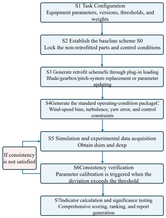
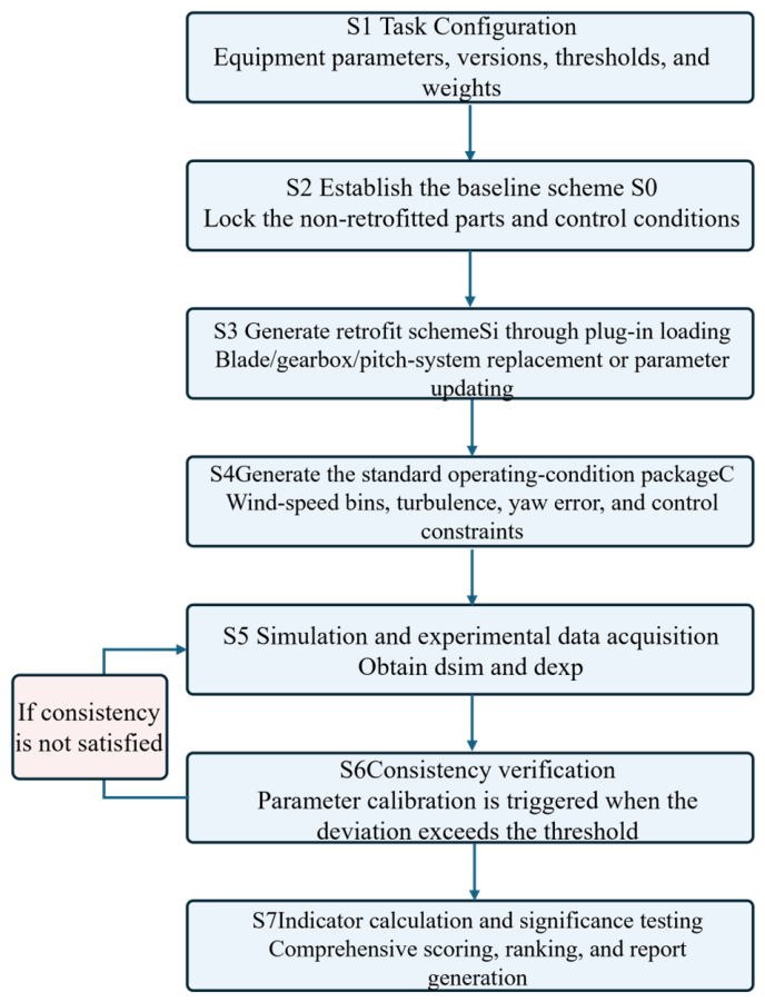
The proposed evaluation procedure comprises seven sequential stages: task configuration, baseline modeling, plug-and-play retrofit integration, standardized operational package generation, simulation and experimental data acquisition, consistency verification and parameter calibration, and multi-metric calculation with comprehensive ranking, as shown in Figure 2. The critical contribution, however, lies not in the procedural sequence itself, but rather in the seamless integration of multi-source data into a unified evaluation pipeline. This integration is achieved through standardized configuration files, identical operational packages, and consistent metric definitions [22,23,24].

Figure 2. Standardized testing and comparative evaluation workflow.

During the task configuration stage, several critical parameters must be predefined: the equipment model, rated specifications, control strategy version, interface exchange variables, sampling frequencies, time synchronization methods, operational binning criteria, validation thresholds, multi-metric weights, and sources of uncertainty. To enhance process traceability, the configuration file should rigorously document version numbers and configuration summaries to facilitate subsequent verification [19].

During the simulation and empirical data acquisition phase, the temporal resolution and indexing frameworks of the model outputs and measured data must be strictly aligned. For critical operational conditions, validation via experimental, hardware-in-the-loop, or bench testing is prioritized. Conversely, large-scale scheme screening relies primarily on computational simulations. This methodology yields a robust hybrid strategy characterized by extensive simulation coverage coupled with rigorous empirical validation [25,26,27,28]. In the present numerical demonstration, the physical data branch is inactive; the consistency check uses candidate-model outputs and a fixed numerical reference dataset only.

2.3. Data Preprocessing and Consistency Verification Model

To ensure direct comparability between simulation outputs and empirical data, a standardized preprocessing protocol must be implemented prior to metric calculation. This procedure encompasses temporal resampling, time alignment, outlier removal, missing data imputation, and environmental correction. For critical signal channels—including power, torque, rotational speed, pitch angle, temperature, and vibration—outliers are identified using a hybrid strategy that integrates statistical thresholding with empirical engineering rules. Additionally, variables highly sensitive to fluctuations in air density or ambient temperature must be normalized to standard environmental conditions. Specifically, outliers are screened using a Hampel rule with a seven-sample centered window and a threshold of 3 × 1.4826 MAD, followed by engineering range checks. State change excursions are retained when they correspond to prescribed operating transitions. Missing segments of no more than two consecutive samples are filled by linear interpolation, whereas longer gaps are excluded from the corresponding operating condition bin. The present illustrative numerical dataset is complete, so the missing data branch is not invoked in the reported results.

The consistency verification module formulates a deviation vector comprising errors in the power curve, torque response, pitch dynamics, thermal variations, and vibration signatures, while also establishing corresponding allowable thresholds. If any critical validation metric exceeds its predefined limit, parameter calibration is initiated. Subsequently, system parameters—such as transmission efficiency, damping coefficients, mechanical backlash, and actuator dynamics—are iteratively refined until the simulated and empirical data converge to satisfy the requisite consistency across all key operational conditions [29,30,31]. In the present case, these equations are used as a numerical consistency check framework; no physical reference dataset is used.

$${\tau }^{*}=\arg {\max }_{\tau \in [{\tau }_0,{\tau }_1]}\mathrm{Corr}\left(D_{sim}(t),D_{rcf}(t+\tau )\right)$$

(1)

$$v_{std}=v{\left({\displaystyle \frac{\rho }{{\rho }_0}}\right)}^{1/3}$$

(2)

$${\delta }_k=\max \left\{E_{RMSE,k},E_{MAE,k},E_{L_{\infty },k},E_{dyn,k}\right\}$$

(3)

$${\theta }^{(n+1)}={\theta }^{(n)}-\alpha {\nabla }_{\theta }J\left({\theta }^{(n)}\right)$$

(4)

where ${\tau }^{*}$ denotes the optimal alignment time delay determined by correlation analysis. V_std is the converted wind speed under standard air density conditions. E_k is the consistency evaluation value of the k-th verification quantity. J(θ) is the parameter vector to be calibrated, and is the calibration objective function. In the present numerical demonstration, the reference dataset in the consistency comparison is numerical rather than experimental or physical.

Uncertainty is retained as a general framework capability. When repeated measurements or a prescribed stochastic input model are available, measurement, environmental, and modeling contributions can be combined using Equation (8). Because the present illustrative dataset includes neither repeated physical measurements nor a prescribed stochastic parameter distribution model, quantitative uncertainty propagation, confidence intervals, and statistical significance testing are not reported for the current case [4,16].

$$AEP={\displaystyle \sum _{i}P}(v_i)f(v_i)T$$

(5)

$$\mathrm{\Delta }AEP={\displaystyle \frac{AE{P}_i-AE{P}_0}{AE{P}_0}}\times 100\%$$

(6)

$$DEL={\left({\displaystyle \frac{{\displaystyle \sum _r{n}_r}{S}_r^m}{N_{\mathrm{ref}}}}\right)}^{1/m}$$

(7)

$$u_c(y)=\sqrt{u_{\mathrm{num}}^2+u_{\mathrm{env}}^2+u_{\mathrm{model}}^2+u_{\mathrm{meas}}^2}$$

(8)

where the power output in the (i)-th wind speed bin and the corresponding wind frequency occurrence are used to calculate AEP, T is the number of hours in the evaluation period; (G) denotes the relative gain; DEL is the damage equivalent load, and the combined standard uncertainty is denoted by the uncertainty term in Equation (8). For DEL, S_r is the load range in rainflow bin r, n_r is the corresponding number of cycles, m is the Wöhler exponent, and N_ref is the reference number of cycles. A physical DEL requires cycle-resolved structural-load histories. Because the present case uses response-level fatigue load proxy data rather than cycle-resolved histories, the results in Section 4 are reported as fatigue load-proxy changes rather than physically calculated DEL values.

For the present numerical demonstration, scheme-level response indicators are obtained by time-averaging the reported fatigue load proxy, peak load proxy, transmission efficiency proxy, gearbox temperature, vibration RMS, and reliability proxy time series, and relative changes are calculated with respect to S0 as defined in Equation (9).

$$\begin{array}{l}{L}_{F,i}={\displaystyle \frac{1}{N}}{\displaystyle \sum _{t=1}^N{L}_{F,i}}(t),\hspace{1em}\mathrm{\Delta }{L}_{F,i}={\displaystyle \frac{L_{F,i}-L_{F,0}}{L_{F,0}}}\times 100\%\\ L_{P,i}={\displaystyle \frac{1}{N}}{\displaystyle \sum _{t=1}^N{L}_{P,i}}(t),\hspace{1em}\mathrm{\Delta }{L}_{P,i}={\displaystyle \frac{L_{P,i}-L_{P,0}}{L_{P,0}}}\times 100\%\\ {\eta }_i={\displaystyle \frac{1}{N}}{\displaystyle {\displaystyle \sum _{t=1}^N}{\eta }_i}(t),\hspace{1em}{T}_i={\displaystyle \frac{1}{N}}{\displaystyle {\displaystyle \sum _{t=1}^N}{T}_i}(t)\\ V_{RMS,i}={\displaystyle \frac{1}{N}}{\displaystyle {\displaystyle \sum _{t=1}^N}{V}_{RMS,i}}(t),\hspace{1em}{R}_i={\displaystyle \frac{1}{N}}{\displaystyle {\displaystyle \sum _{t=1}^N}{R}_i}(t)\end{array}$$

(9)

In Equation (9), ${\bar{L}}_{F,i}$ and ${\bar{L}}_{P,i}$ denote the fatigue load and peak load proxy time series for scheme i; ${\bar{\eta }}_i$, ${\bar{T}}_i$, $V_{RMS,i}\left(t\right)$, and ${\bar{R}}_i$ denote the transmission efficiency proxy, gearbox temperature, vibration RMS, and reliability proxy time series; and N is the number of representative daily samples. The response-level proxy traces are fixed illustrative numerical inputs of the demonstrative dataset rather than outputs of a manufacturer-resolved physical damage or failure model. The reliability quantity is dimensionless and is not interpreted as a failure probability [32,33,34].

2.4. Construction of a Multidimensional Indicator System

Although a particular retrofit scheme may enhance energy capture capabilities, concurrent increases in blade root loads, drivetrain vibrations, or actuator temperatures can elevate long-term operational risks, potentially negating short-term economic gains. To address these inherent trade-offs, this study formulates an evaluation matrix encompassing four primary metric domains: revenue, loads, efficiency, and reliability. Explicit evaluation criteria and constraint logic are established for each domain, with the detailed metric framework presented in Table 2 [35,36].

Table 2. Proposed evaluation indicator system.

Indicator Category	Representative Indicators	Evaluation Direction	Engineering Significance
Revenue-related indicators	AEP gain; power curve variation	Larger is better	Measures the improvement in energy capture capability and direct revenue
Load-related indicators	DEL variation when cycle-resolved load histories are available; fatigue load and peak load proxy variations in the present case	Smaller is better	Reflects structural safety, life consumption, and fatigue risk
Efficiency-related indicators	Transmission efficiency; control response efficiency	Larger is better	Characterizes the improvement in energy conversion and actuation performance
Reliability-related indicators	Temperature rise margin; vibration characteristics; reliability proxy indicator	More stable is better	Supports long-term operational reliability assessment and acceptance conclusions

Specifically, revenue metrics evaluate the retrofit’s direct contribution to power generation capabilities. Load metrics assess potential degradations in structural safety margins. Efficiency metrics gauge the overall efficacy of energy conversion and control execution, while reliability metrics characterize long-term operational conditions and failure risks. In practical applications, the weighting logic must adapt to the evaluation scenario: reliability and load metrics necessitate stricter constraint priorities during project acceptance, whereas revenue and efficiency metrics can be prioritized during preliminary scheme screening.

During the comprehensive decision-making stage, feasibility screening is initially conducted, followed by data normalization and weighted ranking. This screening process eliminates candidate schemes for which critical constraint metrics—such as mechanical loads, thermal variations, and vibrations—exceed permissible thresholds. Consequently, this prevents the flawed adoption of retrofits that enhance energy production at the expense of safety margins. Schemes passing this initial screening are subsequently subjected to comprehensive scoring, yielding ranking results with enhanced engineering interpretability [37,38,39]. The comprehensive score can then be formulated as follows: for benefit indicators, min–max normalization is performed as x′ = (x − x_min)/(x_max − x_min); for cost indicators, x′ = (x_max − x)/(x_max − x_min). In the present case, x_min and x_max are calculated over the feasible retrofit candidates S1–S3, while S0 is retained only as the baseline reference. The weighted score is then calculated using Equation (10).

$${x^{\prime }}_{ij}=\left\{\begin{array}{ll}{\displaystyle \frac{x_{ij}-x_j^{\min }}{x_j^{\max }-x_j^{\min }}},\hfill & j\in \mathcal{B},\hfill \\ [6pt]{\displaystyle \frac{x_j^{\max }-x_{ij}}{x_j^{\max }-x_j^{\min }}},\hfill & j\in \mathcal{C},\hfill \end{array}\right.\hspace{1em}\hspace{1em}{\mathrm{Score}}_i={\displaystyle {\displaystyle \sum _{j=1}^m}{w}_j}{x^{\prime }}_{ij},\hspace{1em}\hspace{1em}{\displaystyle {\displaystyle \sum _{j=1}^m}{w}_j}=1$$

(10)

where $x_{ij}$ is the original value of the indicator for scheme; ${x^{\prime }}_{ij}$ is the corresponding normalized value; $x_j^{\mathrm{m}\mathrm{i}\mathrm{n}}$ and $x_j^{\mathrm{m}\mathrm{a}\mathrm{x}}$ are the minimum and maximum values of the indicator among the candidate retrofit schemes that pass the feasibility screening; $\mathcal{B}$ and $\mathcal{C}$ denote the sets of benefit-type and cost-type indicators, respectively; $w_j$ is the weight assigned to indicator j; m is the total number of indicators; and ${\mathrm{Score}}_i$ is the composite score of scheme i. In the present case, the minimum and maximum values are calculated only among the feasible candidate retrofit schemes S1–S3, while the baseline scheme S0 is used only as the reference and is excluded from the min–max normalization. The case-specific weight vector and its engineering basis are reported in Section 3.3, and alternative priority scenarios are examined in Section 4.4.

3. Demonstrative Case Setup and Data Processing

3.1. Equipment Object, Candidate Schemes, and Operating Condition Settings

To validate the engineering applicability of the proposed method, a case study is conducted using a generic numerical configuration representing a 2.5 MW-class doubly fed induction generator (DFIG) wind turbine. The reference configuration serves as the baseline scheme (S0). Assuming the tower, primary control framework, and major structural parameters remain unaltered, three candidate retrofit schemes are defined: blade replacement (S1), gearbox optimization (S2), and a pitch system upgrade (S3). These schemes are interchangeably integrated into a unified model via plug-and-play interfaces and evaluated under strictly identical operational packages, as summarized in Table 3.

Table 3. Typical retrofit objects and aggregate scheme definitions.

Item	S0 Baseline	Scheme-Level Change Used in the Numerical Demonstration	Engineering Interpretation
Rated turbine power	2.5 MW	Unchanged	Common rated-power boundary
Rotor diameter/cut-in/rated/cut-out wind speed	121 m/3/11/25 m/s	Unchanged	Common operating boundary
Reference configuration	Generic 2.5 MW-class doubly fed wind turbine	No manufacturer-specific model or controller	Defines the scope as an illustrative numerical case
S1: Blade replacement	Baseline blade/aerodynamic representation	Improved low-/medium-wind aerodynamic and power curve response; non-retrofitted settings unchanged	Energy-oriented retrofit
S2: Gearbox optimization	Baseline drivetrain representation	Reduced aggregate drivetrain loss; improved efficiency, thermal, and vibration response	Balanced drivetrain-oriented retrofit
S3: Pitch system upgrade	Baseline pitch/control response	Improved aggregate pitch/control response for load mitigation; rated power boundary unchanged	Load-mitigation/control-response retrofit

The scheme definitions for S1–S3 are summarized in Table 3 at the aggregate modeling level actually used in this numerical demonstration. Manufacturer-specific actuator, controller, blade, or gearbox design parameters are not claimed because they were not part of the original case calculation.

The standardized operational package comprises wind speed bins, air density, turbulence intensity, and yaw errors. In this study, standard wind speed bins ranging from 4 to 15 m/s are selected as the primary interval for power curve evaluation. To establish representative daily operational data, 96 time series samples—each with a 15 min duration—are generated. Additionally, nine critical operational points are extracted to facilitate numerical consistency verification.

3.2. Data Sources and Preprocessing Procedure for the Demonstrative Equipment

The case study dataset comprises two primary components: power curve and load evaluation data under standard operational conditions, and representative daily time series data. The latter encompasses environmental variables—such as wind speed, air density, turbulence intensity, and yaw errors—alongside scheme-specific quantities, including power, torque, pitch angle, gearbox temperature, vibration root-mean-square (RMS), fatigue load proxy, peak load proxy, transmission efficiency proxy, and reliability proxy values. Prior to metric calculation, a rigorous data preprocessing protocol is executed, encompassing temporal alignment, outlier removal, air density normalization, and consistency checking. The representative day contains 96 consecutive 15-min numerical samples, and the same fixed environmental sequence is used for S0–S3. For the current case, candidate outputs are aligned with a fixed numerical reference, and wind speed is normalized to standard air density according to Equation (2). No field, bench, or HIL measurement dataset, manufacturer-specific solver, proprietary controller, or manufacturer-specific aerodynamic database is used.

The critical validation metrics encompass deviations in the power curve, torque response, pitch dynamics, thermal variations, and vibration signatures. In the general framework, if a metric exceeds its prescribed threshold, the corresponding model or response parameters may be calibrated. In the present case, Table 4 provides an illustrative numerical consistency check example only; these values do not constitute physical calibration evidence.

Table 4. Illustrative numerical consistency check example before and after correction.

Verification Quantity	Before Correction	After Correction
Power RMSE/%	5.8	2.4
Torque response RMSE/%	7.1	3.0
Pitch dynamic MAE/°	0.64	0.28
Temperature RMSE/°C	4.5	1.9
Vibration feature error/%	8.2	3.4

3.3. Case-Specific Feasibility Constraints and Scoring Settings

The feasibility thresholds used in this numerical demonstration are listed in Table 5. They are illustrative scenario settings selected only to demonstrate the two-stage decision logic and are not proposed as OEM, certification, or universal acceptance limits. A real retrofit project must replace them with project-specific design allowables, component limits, and contractual acceptance criteria. With the thresholds defined in Table 5, all three candidate schemes pass the illustrative screen and proceed to weighted ranking.

Table 5. Feasibility thresholds used in the numerical demonstration.

Constraint Indicator	Illustrative Threshold	Decision Rule	Case-Study Status
Fatigue = load proxy change	≤+8%	Reject if exceeded	S1/S2/S3 pass
Peak load proxy change	≤+5%	Reject if exceeded	S1/S2/S3 pass
Maximum gearbox temperature	≤95 °C	Reject if exceeded	S1/S2/S3 pass
Mean vibration RMS	≤2.5 mm/s	Reject if exceeded	S1/S2/S3 pass
Mean reliability proxy	≥0.75	Reject if below threshold	S1/S2/S3 pass

For the current ranking configuration, the indicator order is [AEP gain, fatigue load proxy change, peak load proxy change, efficiency proxy change, average gearbox temperature, vibration RMS, reliability proxy]. The corresponding weights are 0.25, 0.15, 0.20, 0.20, 0.05, 0.05, and 0.10, respectively; the same values are reported in the scoring breakdown in Table 6.

Table 6. Normalized indicators, weights, and weighted score contributions.

Indicator	Weight	S1 Norm.	S1 Weighted	S2 Norm.	S2 Weighted	S3 Norm.	S3 Weighted
AEP gain	0.25	1.000	0.250	0.336	0.084	0.000	0.000
Fatigue proxy	0.15	0.000	0.000	0.628	0.094	1.000	0.150
Peak proxy	0.20	0.000	0.000	0.368	0.074	1.000	0.200
Efficiency proxy	0.20	0.000	0.000	1.000	0.200	0.116	0.023
Mean gearbox temp.	0.05	0.000	0.000	1.000	0.050	0.416	0.021
Vibration RMS	0.05	0.000	0.000	1.000	0.050	0.677	0.034
Reliability proxy	0.10	0.000	0.000	1.000	0.100	0.726	0.073
Total/Score	1.00	—	0.250	—	0.652	—	0.500

AEP, efficiency, and reliability are benefit indicators; fatigue load proxy change, peak load proxy change, temperature, and vibration are cost indicators. The adopted weight vector is an illustrative balanced engineering scenario rather than a universal standard or an expert-elicited optimum. It assigns 25% to energy benefit, 35% to the two load-related proxies, 20% to efficiency, and 20% in total to temperature, vibration, and reliability. The sensitivity analysis in Section 4.4 deliberately varies these priorities to show that the final ranking is weight-dependent.

4. Results and Discussion

4.1. Evaluation of Different Modular Performance Test Solutions

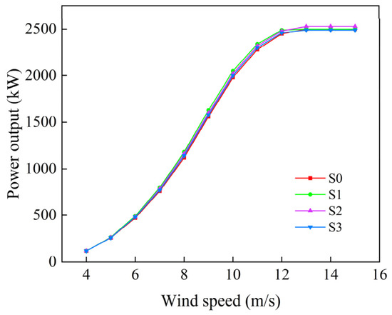
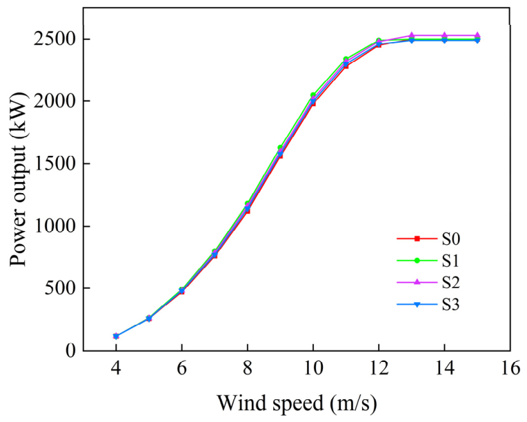
Figure 3 illustrates the standard power production of the candidate schemes across various wind speeds. The power gain achieved by the blade replacement scheme (S1) is most pronounced in the low-to-medium wind speed regimes, particularly between 6 and 10 m/s. The upward shift in its power curve relative to the baseline (S0) indicates that aerodynamic optimization primarily enhances energy capture capabilities below the rated wind speed. Meanwhile, the gearbox optimization scheme (S2) yields a more modest power increase but maintains a stable gain across medium-to-high wind speeds, demonstrating that enhanced transmission efficiency effectively mitigates mechanical losses. Furthermore, the power curve for the pitch system upgrade (S3) closely aligns with that of S0, confirming that this scheme aims primarily to mitigate load fluctuations via improved control responses rather than significantly increasing power output.

Figure 3. Comparison of power curves under standard operating conditions.

Based on the wind speed bin frequencies, the AEP of the baseline scheme (S0) is calculated to be 12.79 GWh. The AEP values for schemes S1, S2, and S3 are 13.21, 12.98, and 12.87 GWh, yielding relative gains of 3.32%, 1.52%, and 0.61%, respectively. From the perspective of revenue metrics, S1 demonstrates the most substantial impact on power generation enhancement. However, within the broader context of retrofit evaluation, AEP merely quantifies energy capture; it fails to account for potential adverse shifts in structural loads, drivetrain thermal variations, or reliability risks. Consequently, a multidimensional assessment is imperative. This evaluation is further conducted by incorporating representative daily time series responses, load proxy metrics, thermal and vibration signatures, and a final comprehensive score.

4.2. Effects of Working Condition Characteristics on Power Generation

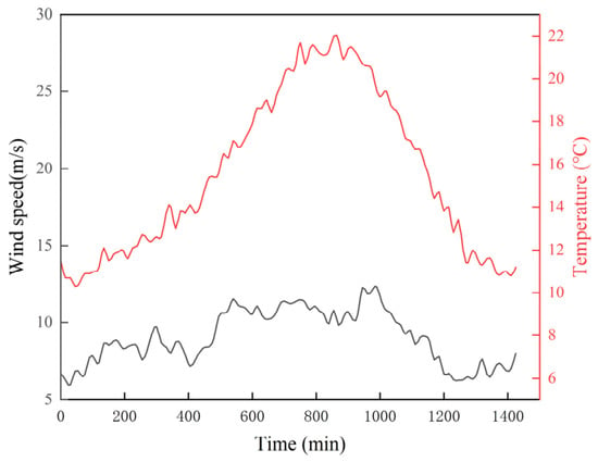
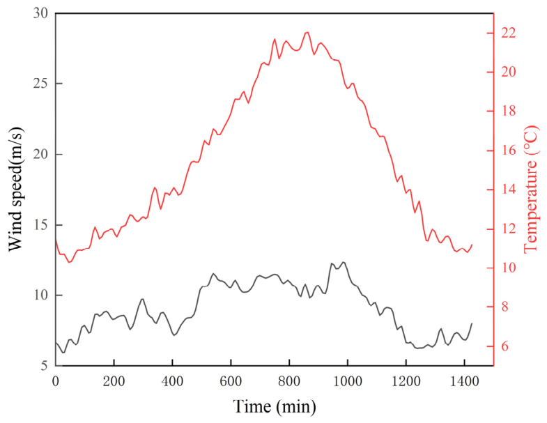
To evaluate the dynamic responses of the candidate schemes under unsteady operational conditions, 96 representative daily time series samples were constructed. Each sample comprises 15-min intervals, cumulatively spanning a full 24-h period (1440 min). Figure 4 illustrates the temporal variations in wind speed and ambient temperature for this representative day. Specifically, wind speed fluctuates between 5.96 m/s and 12.32 m/s (mean: 9.02 m/s; standard deviation: 1.76 m/s). This profile effectively encompasses typical operational regimes, including low-to-medium wind speeds, near-rated conditions, and transient wind speed dips. Concurrently, ambient temperatures range from 10.3 °C to 22.0 °C, averaging 15.54 °C. Furthermore, the mean air density is established at 1.215 kg/m³, the average turbulence intensity is 0.113, and yaw errors are predominantly distributed between −6.08° and 7.13°. These rigorously defined conditions not only capture the stochastic fluctuations inherent in natural wind environments but also preclude evaluation biases stemming from inconsistent boundary conditions across the various schemes.

Figure 4. Variation in representative daily wind speed and ambient temperature at different times.

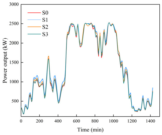
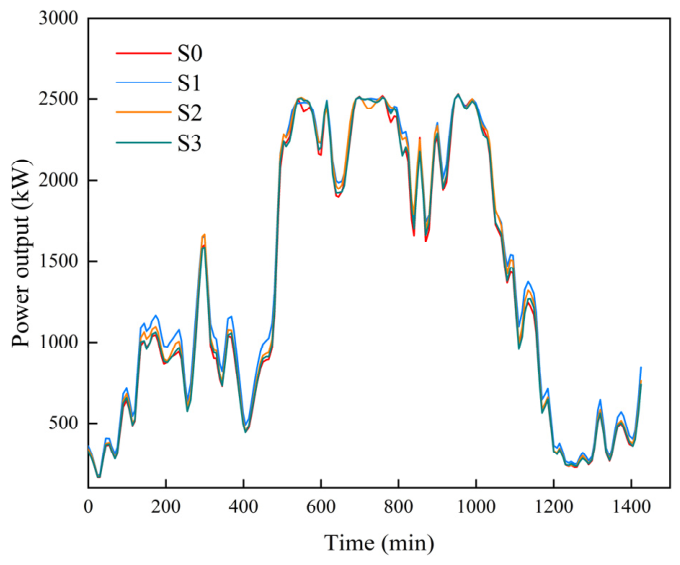
Figure 5 illustrates the dynamic power responses of the evaluated schemes when subjected to identical environmental inputs. The four power curves exhibit synchronous fluctuations corresponding to wind speed variations, frequently approaching the 2.5 MW rated power threshold during high wind speed intervals, particularly between the 500th and 1000th minutes. Statistically, the mean daily power outputs for schemes S0, S1, S2, and S3 are 1320.7, 1386.1, 1352.6, and 1328.2 kW, respectively. Relative to the baseline (S0), S1 achieves the highest mean power increment of 65.4 kW (a 4.95% enhancement). Schemes S2 and S3 yield more modest increases of 31.9 kW (2.41%) and 7.5 kW (0.56%), respectively. These findings seamlessly align with the preceding wind speed bin analysis; specifically, S1 delivers the most substantial contribution to revenue metrics, followed by S2, whereas the overall power gain from S3 remains marginal.

Figure 5. Comparison of power generation at different times.

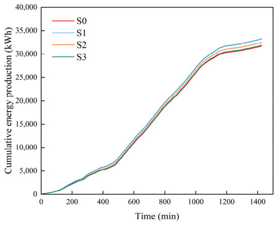
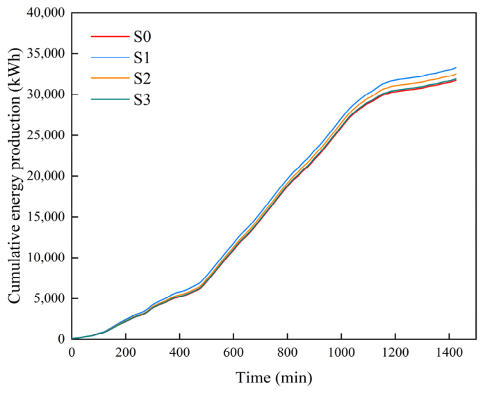
Figure 6 further illustrates the trajectory of cumulative energy production throughout the representative day. Because cumulative energy is the temporal integral of the power time series, performance disparities among the schemes expand progressively during high-wind speed and near-rated operational intervals. By the end of the 24 h period, the total energy yields for schemes S0, S1, S2, and S3 reach 31,697.1, 33,266.8, 32,461.9, and 31,875.9 kWh, respectively. Relative to the baseline (S0), S1, S2, and S3 achieve absolute increments of 1569.7 kWh (a 4.95% increase), 764.8 kWh (2.41%), and 178.8 kWh (0.56%), respectively. Evidently, the blade replacement scheme (S1) delivers the most substantial short-term energy gain under these representative conditions. However, since this advantage stems primarily from enhanced aerodynamic capture capabilities, it remains imperative to further investigate whether such benefits incur hidden penalties in structural loads or system reliability.

Figure 6. Comparison of cumulative energy production at different times.

4.3. Performance Investigation of Wind Turbine Retrofit Schemes

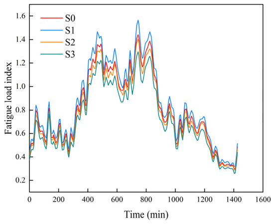
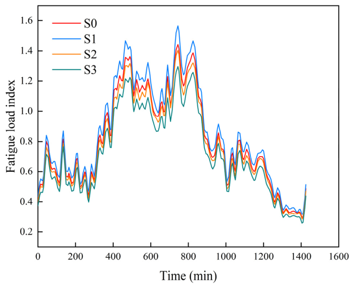
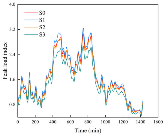
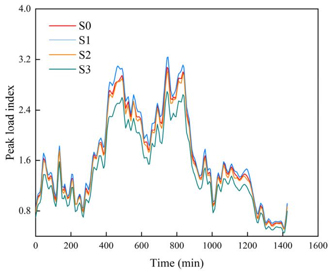
Figure 7 and Figure 8 depict the time series responses of the representative daily fatigue load and peak load proxy metrics, respectively. The fatigue load proxy metric primarily reflects the impact of continuous cyclic loading on structural life consumption, whereas the peak load proxy metric captures the extreme transient impacts induced by short-term gusts, yaw errors, and control interventions. As illustrated in Figure 7, the fatigue load across all schemes escalates with increasing wind speed, exhibiting a pronounced surge during the high wind speed interval between the 400th and 900th minutes. Statistically, the mean fatigue load proxy metrics for schemes S0, S1, S2, and S3 are 0.870, 0.924, 0.837, and 0.785, respectively. Relative to the baseline (S0), scheme S1 exhibits a 6.11% increase, whereas S2 and S3 demonstrate reductions of 3.90% and 9.83%, respectively. These findings indicate that while S1 enhances power generation, it concurrently exacerbates the risk of fatigue damage. Conversely, S3 achieves the most substantial fatigue load suppression via pitch control optimization. These two quantities are response-level comparative proxies in the present numerical dataset and are not interpreted as physically calculated DEL values or certified extreme load values.

Figure 7. Proxy index of fatigue load at different times.

Figure 8. Proxy index of peak load at different times.

Regarding the peak load outcomes, the mean peak load proxy metrics for schemes S0, S1, S2, and S3 are 1.674, 1.736, 1.636, and 1.465, respectively. Relative to the baseline (S0), scheme S1 exhibits a 3.72% increase, whereas S2 and S3 demonstrate reductions of 2.25% and 12.49%, respectively. The peak load curves display numerous local maxima during periods of rapid wind speed fluctuations, indicating that this metric is highly sensitive to short-term environmental disturbances. Notably, the elevated peak load of S1 signifies that its revenue enhancement involves an inherent trade-off, potentially compromising the safety margins of critical components such as the blade root, main shaft, and drivetrain. Conversely, S3 achieves the most substantial peak load reduction, demonstrating that the pitch system upgrade effectively mitigates extreme transient impacts. Consequently, this scheme is particularly advantageous for high turbulence environments, aging turbines, or scenarios with constrained structural load margins. Although S2 is not the optimal load mitigation strategy, its reduced load level relative to S0 confirms that gearbox optimization does not introduce supplementary load-related risks.

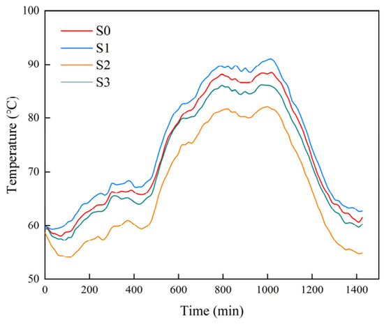
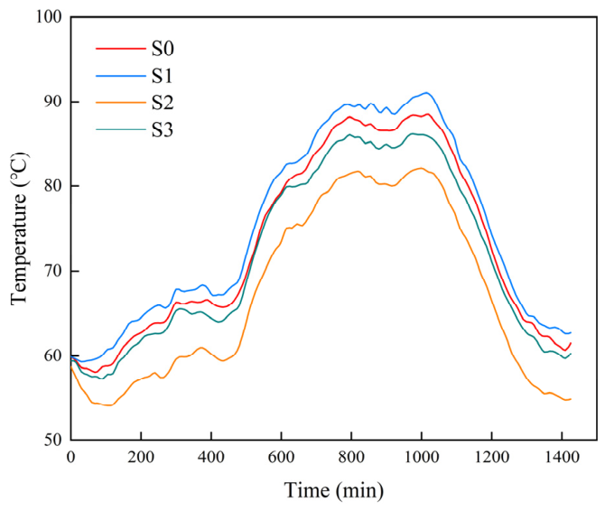
Beyond structural loads, thermal variations and vibration signatures serve as critical metrics for evaluating the operational health of the drivetrain. As illustrated in Figure 9, the gearbox temperature exhibits pronounced thermal inertia in response to fluctuations in wind speed and power output. During periods of high-power generation, the temperature escalates gradually, subsequently subsiding at a slow rate once the wind speed decreases. Statistically, the mean gearbox temperatures for schemes S0, S1, S2, and S3 are 73.20 °C, 74.95 °C, 67.24 °C, and 71.74 °C, respectively, with corresponding maximum temperatures reaching 88.5 °C, 91.0 °C, 82.1 °C, and 86.2 °C. Relative to the baseline (S0), the mean temperature of S1 increases by 1.75 °C, whereas S2 and S3 exhibit reductions of 5.96 °C and 1.46 °C, respectively. The thermal mitigation achieved by S2 is particularly prominent and is consistent with the aggregate reduction in drivetrain losses used to represent the S2 retrofit in this numerical case.

Figure 9. Temperature comparison of gearbox under different time.

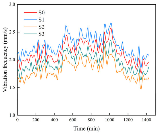
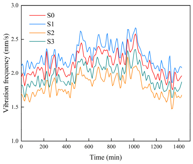
Figure 10 illustrates the time series responses of the vibration root-mean-square (RMS) values. The vibration levels exhibit localized surges during high wind speed intervals and rapid power transients, aligning consistently with load fluctuations and the dynamic excitation of the drivetrain. Statistically, the mean vibration RMS values for schemes S0, S1, S2, and S3 are 2.127, 2.260, 1.817, and 1.960 mm/s, respectively. Relative to the baseline (S0), scheme S1 exhibits an increase of 0.133 mm/s (6.27%), whereas S2 and S3 demonstrate substantial reductions of 0.311 mm/s (14.60%) and 0.167 mm/s (7.84%), respectively. The elevated vibration level in S1 corroborates its enhanced power capture and correspondingly higher structural loads. Conversely, S2 achieves the most pronounced vibration suppression, indicating improved drivetrain-state behavior under the aggregate S2 representation. Furthermore, the vibration reduction observed in S3 is consistent with its load mitigation and control response objective.

Figure 10. Comparison of vibration RMS timing.

4.4. Evaluation of Multi-Index

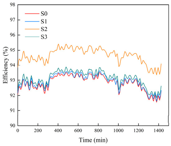
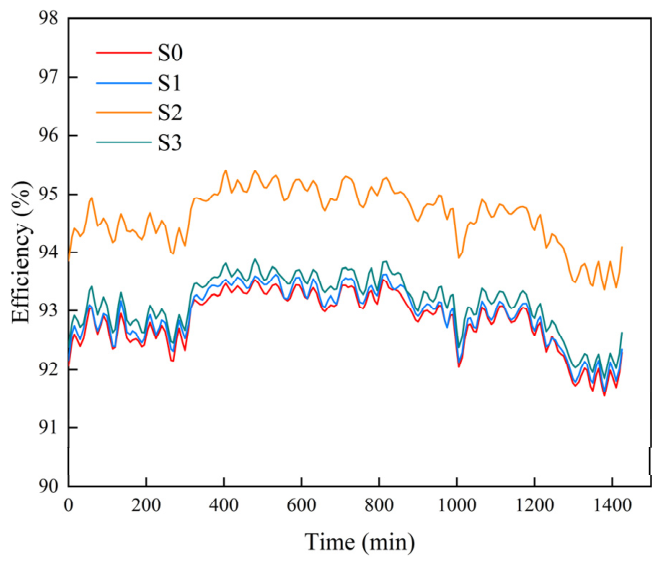
Figure 11 illustrates the time series responses of the transmission efficiency proxy metric throughout the representative day. Statistically, the mean efficiencies for schemes S0, S1, S2, and S3 are 92.562%, 92.663%, 94.363%, and 92.860%, respectively. Notably, S2 exhibits an increase of 1.80 percentage points relative to the baseline (S0) and maintains the highest efficiency level across the entire operational period, fluctuating between 93.147% and 95.224%. In contrast, schemes S1 and S3 yield marginal increments of only 0.101 and 0.298 percentage points, respectively. These findings underscore the distinct physical mechanisms driving each retrofit strategy: while blade replacement primarily enhances aerodynamic energy capture and the pitch system upgrade focuses on load mitigation and control response, the S2 retrofit is represented by reduced aggregate drivetrain losses together with improved thermal and vibration responses. Consequently, S2 achieves a fundamentally more stable and pronounced efficiency enhancement.

Figure 11. Time series comparison of transmission efficiency proxy index.

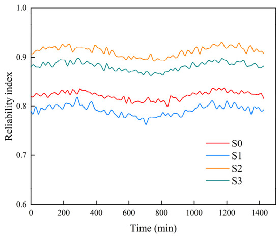
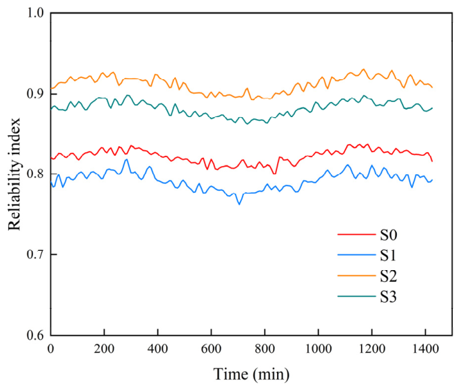
Figure 12 illustrates the temporal variation in the supplied dimensionless reliability proxy metric. This comparative proxy is not interpreted as a failure probability. Statistically, the mean reliability metrics for schemes S0, S1, S2, and S3 are 0.8065, 0.7704, 0.9125, and 0.8735, respectively, following a descending order of S2 > S3 > S0 > S1. Relative to the baseline (S0), scheme S1 exhibits a 4.49% decrease. This indicates that while S1 enhances power generation revenue, the concurrent escalations in structural loads, thermal variations, and vibration signatures compromise its long-term operational reliability. Conversely, S2 demonstrates a notable 13.13% improvement, underscoring the comprehensive advantages of gearbox optimization in mitigating thermal variations, suppressing vibrations, and preserving load boundaries. Furthermore, S3 achieves an 8.30% increase, which is primarily attributable to substantial reductions in both fatigue and peak loads. Ultimately, these reliability outcomes reinforce the critical premise: the evaluation of retrofit strategies must transcend exclusive reliance on AEP gains and rigorously incorporate component health and lifecycle risks.

Figure 12. Time series comparison of reliability proxy index.

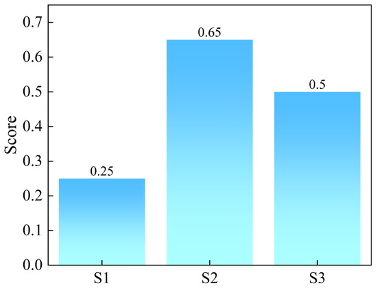
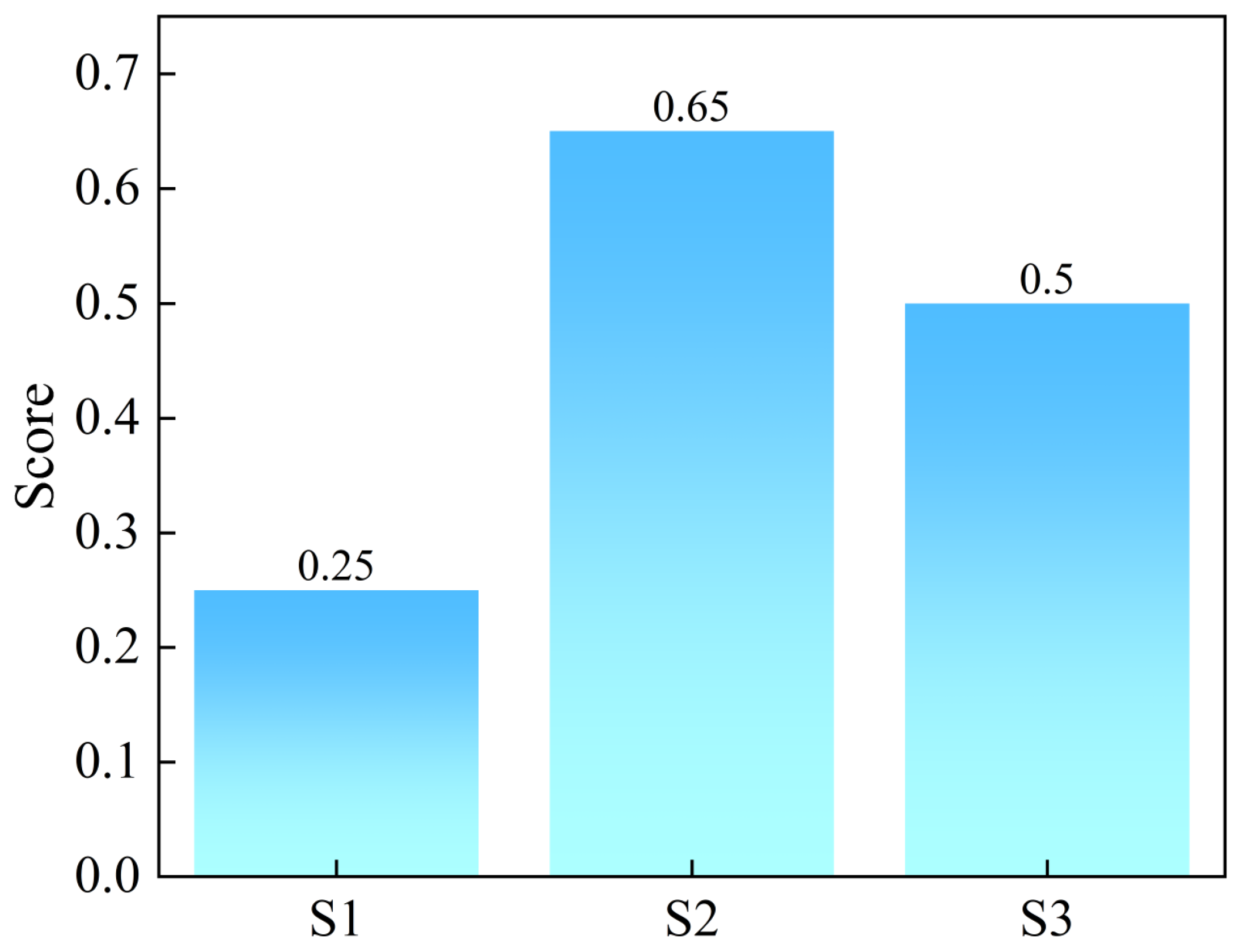
The S2 score is reconstructed from the unrounded normalized values in Table 6. Its weighted contributions are 0.084, 0.094, 0.074, 0.200, 0.050, 0.050, and 0.100, giving 0.652 (0.65 after rounding). S1 scores 0.250 and S3 scores 0.500. Thus, S2 ranks first under the stated normalization and weight vector, and the ranking order is S2 > S3 > S1, as shown in Table 7.

Table 7. Weight sensitivity analysis.

Priority Scenario	Weight Vector [AEP, Fatigue Proxy, Peak Proxy, Eff. Proxy, Temp., Vib., Rel.]	S1	S2	S3	Rank 1
Current	[0.25, 0.15, 0.20, 0.20, 0.05, 0.05, 0.10]	0.250	0.652	0.500	S2
Energy-dominant	[0.75, 0.03, 0.03, 0.08, 0.02, 0.02, 0.07]	0.750	0.472	0.142	S1
Load-dominant	[0.10, 0.25, 0.30, 0.10, 0.05, 0.05, 0.15]	0.100	0.651	0.725	S3
Reliability/efficiency	[0.15, 0.10, 0.10, 0.20, 0.10, 0.10, 0.25]	0.150	0.800	0.514	S2

The sensitivity analysis demonstrates that the current ranking is not universal. S2 is first under the current and reliability/efficiency configurations; S1 becomes first when AEP is intentionally dominant, and S3 becomes first when load reduction dominates. This confirms that the preferred scheme depends on declared engineering priorities rather than on a universal weight set.

The three retrofit types can have coupled effects in an actual turbine. A blade change can alter aerodynamic torque and therefore the loading transmitted to the drivetrain; a gearbox-oriented retrofit can modify drivetrain losses and thermal/vibration behavior; and a pitch system upgrade can alter transient aerodynamic loading and control response. Because the present case evaluates the three schemes as isolated aggregate modifications, combined S1 + S2, S1 + S3, or S2 + S3 effects should not be inferred by linear addition of the individual results. Combined module interactions require a dedicated component-resolved simulation or physical validation campaign.

Table 8 summarizes the comprehensive evaluation outcomes for each scheme across six key dimensions: revenue, structural loads, operational efficiency, thermal variations, vibration signatures, and overall reliability. Notably, while S1 achieves the highest AEP gain (3.32%), its fatigue load and peak load proxies concurrently increase by 6.11% and 3.72%, respectively. Furthermore, its mean operating temperature and vibration RMS exceed those of the baseline (S0), characterizing S1 as an aggressive revenue-driven strategy that compromises structural and operational margins. In contrast, although the AEP gain of S2 (1.52%) is comparatively modest, it yields reductions in the fatigue load proxy (3.90%) and peak load proxy (2.25%), alongside a 1.801 percentage-point enhancement in the transmission efficiency proxy. Correspondingly, its mean gearbox temperature drops to 67.24 °C, the vibration RMS subsides to 1.817 mm/s, and the reliability proxy reaches 0.9125, demonstrating a favorable balance between energy capture and system health indicators under the present case settings. Conversely, S3 delivers a marginal AEP gain of only 0.61% but achieves substantial reductions in the fatigue load proxy (9.83%) and peak load proxy (12.49%). This profile indicates that S3 is well suited to engineering scenarios where load mitigation, lifespan extension, and operational safety are the primary objectives.

Table 8. Consolidated results for the candidate schemes.

Scheme	AEP (GWh)	ΔAEP (%)	ΔFatigue (%)	ΔPeak (%)	ΔEff. (pp)	Mean Temp. (°C)	Vibration RMS (mm/s)	Reliability	Score
S0 baseline	12.79	0.00	0.00	0.00	0.000	73.20	2.127	0.8065	—
S1 blade replacement	13.21	3.32	6.11	3.72	0.101	74.95	2.260	0.7704	0.25
S2 gearbox optimization	12.98	1.52	−3.90	−2.25	1.801	67.24	1.817	0.9125	0.65
S3 pitch-system upgrade	12.87	0.61	−9.83	−12.49	0.298	71.74	1.960	0.8735	0.50

Figure 13 presents the comprehensive score rankings derived from the current balanced weighting scheme. Scheme S2 attains the highest comprehensive score (0.65), followed by S3 (0.50), whereas S1 registers the lowest score (0.25). Notably, this hierarchy diverges significantly from the ranking predicated solely on AEP gains. This discrepancy underscores the capability of the proposed multi-metric evaluation framework to delineate the crucial distinction between mere optimal financial return and true optimal comprehensive performance. However, the ranking is conditional on the stated normalization and weight vector: the sensitivity analysis in Table 7 shows that S1 becomes first under an energy-dominant scenario, whereas S3 becomes first under a load-dominant scenario.

Figure 13. Comprehensive score ranking of different technical solutions under the current weight vector.

5. Conclusions

Based on the proposed modular performance testing and comparative evaluation methodology, this study conducted a demonstrative numerical case study on retrofit schemes for a generic 2.5 MW-class wind turbine. Three candidate schemes were comparatively analyzed using a standardized operational package, representative daily time series samples, numerical consistency checks, and a multi-metric comprehensive evaluation framework. The results indicate that the blade replacement scheme (S1) demonstrates the most substantial revenue enhancement capabilities. Specifically, S1 achieves an annual AEP gain of 3.32% and a daily cumulative energy increase of 1569.7 kWh relative to the baseline (S0). However, its fatigue load and peak load proxies increase by 6.11% and 3.72%, respectively. Furthermore, its mean operating temperature and vibration levels rise concurrently, characterizing S1 as an aggressive, revenue-driven strategy constrained by notable operational risks. In contrast, although the gearbox optimization scheme (S2) yields a more modest AEP gain of 1.52%, it achieves a 1.801 percentage-point increase in the transmission efficiency proxy, a 5.96 °C reduction in mean temperature, and a 14.60% decrease in vibration root-mean-square. Consequently, its reliability proxy reaches 0.9125, and its comprehensive score is 0.65, so S2 ranks first under the current feasibility thresholds, normalization method, and weight vector. Conversely, the pitch system upgrade (S3) provides a marginal AEP gain but reduces the fatigue load and peak load proxies by 9.83% and 12.49%, respectively. This profile makes S3 suitable for scenarios where load mitigation and life extension priorities dominate.

Overall, the proposed evaluation framework successfully elucidates the trade-offs among revenue, structural load proxies, operational efficiency, and reliability-related indicators under strictly unified boundary conditions. Consequently, it prevents retrofit decisions from being predicated solely on power generation increments. Within the level of evidence provided by the present numerical demonstration, this study provides a preliminary analytical and evaluation basis for the comparative analysis and decision support for wind turbine retrofit schemes.

References

- IEC 61400-1; 2019 Wind Energy Generation Systems—Part 1: Design Requirements. International Electrotechnical Commission (IEC): Geneva, Switzerland, 2019.
- IEC 61400-12-1; 2017 Wind Energy Generation Systems—Part 12-1: Power Performance Measurements of Electricity Producing Wind Turbines. International Electrotechnical Commission (IEC): Geneva, Switzerland, 2017.
- IEC 61400-13; 2015 Wind Turbines—Part 13: Measurement of Mechanical Loads. International Electrotechnical Commission (IEC): Geneva, Switzerland, 2015.
- JCGM 100; 2008 Evaluation of Measurement Data—Guide to the Expression of Uncertainty in Measurement. Joint Committee for Guides in Metrology (JCGM): Paris, France, 2008.
- Lydia, M.; Selvakumar, A.I.; Kumar, S.S.; Kumar, G.E.P. A comprehensive review on wind turbine power curve modeling techniques. Renew. Sustain. Energy Rev. 2014, 30, 452–460. [Google Scholar] [CrossRef] [Scilit]
- Fox, H.; Pillai, A.C.; Friedrich, D.; Collu, M.; Dawood, T. A review of predictive and prescriptive offshore wind farm operation and maintenance. Energies 2022, 15, 504. [Google Scholar] [CrossRef] [Scilit]
- Jonkman, J.; Butterfield, S.; Musial, W.; Scott, G. Definition of a 5-MW Reference Wind Turbine for Offshore System Development; National Renewable Energy Laboratory: Golden, CO, USA, 2009. [Google Scholar]
- Jonkman, J.M.; Buhl, M.L. FAST User’s Guide; National Renewable Energy Laboratory: Golden, CO, USA, 2005. [Google Scholar]
- Bossanyi, E.A. Individual blade pitch control for load reduction. Wind Energy 2003, 6, 119–128. [Google Scholar] [CrossRef] [Scilit]
- Martulli, L.M.; Diani, M.; Sabetta, G.; Bontumasi, S.; Colledani, M.; Bernasconi, A. Critical review of current wind turbine blades’ design and materials and their influence on the end-of-life management of wind turbines. Eng. Struct. 2025, 327, 119625. [Google Scholar] [CrossRef] [Scilit]
- Jung, C.; Sander, L.; Schindler, D. Future global offshore wind energy under climate change and advanced wind turbine technology. Energy Conv. Manag. 2024, 321, 119075. [Google Scholar] [CrossRef] [Scilit]
- Xie, J.; Dong, H.; Zhao, X. Data-driven torque and pitch control of wind turbines via reinforcement learning. Renew. Energy 2023, 215, 118893. [Google Scholar] [CrossRef] [Scilit]
- Pandit, R.; Astolfi, D.; Hong, J.; Infield, D.; Santos, M. SCADA data for wind turbine data-driven condition/performance monitoring: A review on state-of-art, challenges and future trends. Wind Eng. 2023, 47, 422–441. [Google Scholar] [CrossRef] [Scilit]
- Li, J.; Dao, M.H.; Le, Q.T. Data-driven modal parameterization for robust aerodynamic shape optimization of wind turbine blades. Renew. Energy 2024, 224, 120115. [Google Scholar] [CrossRef] [Scilit]
- Kim, C. Development of a physics-based digital twin framework for a 3 MW class wind turbine. Energies 2026, 19, 1088. [Google Scholar] [CrossRef] [Scilit]
- Kennedy, M.C.; O’Hagan, A. Bayesian calibration of computer models. J. R. Stat. Soc. Ser. B 2001, 63, 425–464. [Google Scholar] [CrossRef] [Scilit]
- Tao, F.; Zhang, H.; Liu, A.; Nee, A.Y.C. Digital twin in industry: State-of-the-art. IEEE Trans. Ind. Inform. 2019, 15, 2405–2415. [Google Scholar] [CrossRef] [Scilit]
- NASA-STD-7009A; Standard for Models and Simulations. National Aeronautics and Space Administration (NASA): Washington, DC, USA, 2016.
- IEC 61400-25-2; 2015 Wind Turbines—Part 25-2: Communications for Monitoring and Control of Wind Power Plants—Information Models. International Electrotechnical Commission (IEC): Geneva, Switzerland, 2015.
- Wen, J.; Yu, Y.; Jia, L.; Guo, X.; Jin, Y. Performance analysis and power prediction of iced wind turbines based on CFD-OpenFAST-stacking. Energies 2026, 19, 1194. [Google Scholar] [CrossRef] [Scilit]
- Moriarty, P.J.; Hansen, A.C. AeroDyn Theory Manual; National Renewable Energy Laboratory: Golden, CO, USA, 2005. [Google Scholar]
- IEC TS 61400-26-1; 2019 Wind Energy Generation Systems—Part 26-1: Availability for Wind Energy Generation Systems. International Electrotechnical Commission (IEC): Geneva, Switzerland, 2019.
- Maldonado-Correa, J.; Cuenca-Granda, J.; Torres-Cabrera, J.; Cerda Mejía, G.; Bastidas Barragan, W.D.; Guapulema, R.; Paccha-Herrera, E.; Solano, J.C.; Tapia-Peralta, D.; Benavides, J.; et al. Digital twin technology in wind turbine condition monitoring, predictive maintenance, and RUL estimation: A systematic literature review. Energies 2026, 19, 1477. [Google Scholar] [CrossRef] [Scilit]
- Tautz-Weinert, J.; Watson, S.J. Using SCADA data for wind turbine condition monitoring—A review. IET Renew. Power Gener. 2017, 11, 382–394. [Google Scholar] [CrossRef] [Scilit]
- Jia, N.; Feng, J.; Zuo, Z.; Liu, Z.; Wang, T.; Cai, C.; Li, Q. AI-driven fault detection and O&M for wind turbine drivetrains: A review of SCADA, CMS and digital twin integration. Energies 2026, 19, 1370. [Google Scholar] [CrossRef] [Scilit]
- Bianchini, A.; Bangga, G.; Baring-Gould, I.; Croce, A.; Cruz, J.I.; Damiani, R.; Erfort, G.; Simao Ferreira, C.; Infield, D.; Nayeri, C.N.; et al. Current status and grand challenges for small wind turbine technology. Wind Energy Sci. 2022, 7, 2003–2037. [Google Scholar] [CrossRef] [Scilit]
- Schkoda, R.; Fox, C.; Hadidi, R.; Gevorgian, V.; Wallen, R. Hardware-in-the-Loop Testing of Utility-Scale Wind Turbine Generators; National Renewable Energy Laboratory: Golden, CO, USA, 2016. [Google Scholar]
- Bibo, A.; Panyam, M. Evaluation of dynamic testing of full-scale wind turbine drivetrains with hardware-in-the-loop. Wind Eng. 2022, 46, 1550–1569. [Google Scholar] [CrossRef] [Scilit]
- Tang, H.; Zhang, X.; Hu, B.; Wang, Y.; Shu, X. Wind-YOLO: A lightweight detector for wind turbine damage. Machines 2026, 14, 610. [Google Scholar] [CrossRef] [Scilit]
- Superchi, F.; Moustakis, A.; Pechlivanoglou, G.; Bianchini, A. Can machine learning enhance renewable power forecasts? A study on data-driven methods for solar photovoltaic and wind turbines. Energy 2025, 336, 138396. [Google Scholar] [CrossRef] [Scilit]
- Grosso, P.; D’Elia, G.; Strozzi, M.; Rubini, R.; Cocconcelli, M. On the use of the detectivity parameter for the condition monitoring of wind turbines. Machines 2025, 13, 980. [Google Scholar] [CrossRef] [Scilit]
- Zhang, W.; Vatn, J.; Rasheed, A. Gearbox pump failure prognostics in offshore wind turbine by an integrated data-driven model. Appl. Energy 2025, 380, 124829. [Google Scholar] [CrossRef] [Scilit]
- Li, J.; Yang, P.; Huang, X.; Zhang, L.; Wang, J. Numerical and experimental study on deicing of wind turbine blades by electric heating under complex flow field. Machines 2025, 13, 483. [Google Scholar] [CrossRef] [Scilit]
- Nielsen, J.S.; Clarke, R.; Paquette, J.; Farren, D.; Byrne, A. Risk-based decision modelling for wind turbine leading edge erosion. Energies 2025, 18, 5784. [Google Scholar] [CrossRef] [Scilit]
- Al Hassan, A.; Dao, P.B. Bridging data and diagnostics: A systematic review and case study on integrating trend monitoring and change point detection for wind turbines. Energies 2025, 18, 5166. [Google Scholar] [CrossRef] [Scilit]
- Turnbull, A.; McKinnon, C.; Carroll, J.; McDonald, A. On the development of offshore wind turbine technology: An assessment of reliability rates and fault detection methods in a changing market. Energies 2022, 15, 3180. [Google Scholar] [CrossRef] [Scilit]
- Saaty, T.L. The Analytic Hierarchy Process: Planning, Priority Setting, Resource Allocation; McGraw-Hill: New York, NY, USA, 1980. [Google Scholar]
- Hwang, C.L.; Yoon, K. Multiple Attribute Decision Making: Methods and Applications; Springe: Berlin/Heidelberg, Germany, 1981. [Google Scholar]
- Astolfi, D.; Castellani, F.; Berno, F.; Terzi, L. Numerical and experimental methods for the assessment of wind turbine control upgrades. Appl. Sci. 2018, 8, 2639. [Google Scholar] [CrossRef] [Scilit]
Disclaimer/Publisher’s Note: The statements, opinions and data contained in all publications are solely those of the individual author(s) and contributor(s) and not of MDPI and/or the editor(s). MDPI and/or the editor(s) disclaim responsibility for any injury to people or property resulting from any ideas, methods, instructions or products referred to in the content. |
© 2026 by the authors. Licensee MDPI, Basel, Switzerland. This article is an open access article distributed under the terms and conditions of the Creative Commons Attribution (CC BY) license.