On-Site Dynamic Balancing Optimization of a TPS Rotor System Based on a Hybrid Intelligent Optimization Method

Abstract

To reduce high 1× vibration during staged speed-up of a Turbine Power Simulator (TPS) rotor, a staged incremental on-site balancing method based on a Genetic Algorithm–Salp Swarm Algorithm (GA–SSA) is proposed. SSA is a swarm-intelligence optimizer inspired by salps, gelatinous marine organisms that move collectively in chains. A one-dimensional Timoshenko-beam rotor model with lumped disks and equivalent bearing supports is established and validated using a three-dimensional ANSYS model. From meshes M3 to M4, the equivalent speed associated with the first lateral natural frequency changes by 0.23%. The first three critical-speed errors are 6.75–8.80%, while baseline 1× vibration-amplitude errors remain below 10% and phase errors below 7.1%. Speed-specific influence coefficients are then extracted to formulate a staged incremental balancing model based on the current measured vibration and cumulative correction state. In GA–SSA, the final GA population initializes SSA, and the historical GA best is used as the initial Food. Under equal function-evaluation budgets and 30 paired runs, GA–SSA shows search performance comparable to GA and improves the stability of standalone SSA. On-site tests at 10,358, 25,558, and 38,333 rpm reduce 1× vibration at both rotor ends by 79.0–86.4%, confirming the method’s engineering applicability.

1. Introduction

Rotor systems are widely used in rotating machinery such as aero-engines, gas turbines, turbopumps, compressors, and high-speed motorized spindles [1]. Owing to material inhomogeneity, manufacturing errors, assembly deviations, and operational wear, rotor mass unbalance is difficult to eliminate completely [2,3,4]. During high-speed rotation, the unbalanced mass generates centrifugal excitation synchronous with the rotational speed, which may increase system vibration and noise, aggravate bearing loads, and induce fatigue damage. In severe cases, it may even cause rotor instability or catastrophic failure [5,6,7,8,9,10,11,12]. Therefore, on-site dynamic balancing is an important technique for ensuring the safe operation of high-speed rotors.

Conventional on-site balancing methods mainly include the influence coefficient method [13] and the modal balancing method [14]. The influence coefficient method determines the correction by establishing a linear complex relationship between the correction unbalance and the vibration at the measurement points, and it offers the advantages of straightforward engineering implementation and broad applicability [15,16,17]. However, influence coefficients are usually obtained using trial weights. For flexible rotors undergoing transcritical acceleration, repeated start–stop cycles, trial-weight installations, and remeasurements are often required, which reduces efficiency and increases test risks near critical speeds. In recent years, studies of mechanical systems have increasingly combined physics-based dynamic models with experimentally validated vibration responses for state characterization and vibration-related diagnostics [18]. Finite-element-model-based trial-weight-free or reduced-trial-weight balancing, transient balancing, response matching, state estimation, and multimodal balancing methods have consequently been developed, providing new approaches for reducing the number of on-site tests [19,20,21,22,23,24,25].

Meanwhile, evolutionary and swarm-intelligence algorithms have been increasingly applied to rotor-unbalance parameter identification and correction optimization. Genetic algorithms, differential evolution, particle swarm optimization, grey wolf optimization, and ant colony optimization have been used to solve balancing problems for flexible rotors or rotating assemblies [26,27,28,29], while machine-learning and transfer-learning methods have also been introduced for unbalance identification and state prediction [30,31,32,33]. SSA has a simple structure and requires few control parameters; nevertheless, a standalone algorithm may still exhibit an imbalance between global exploration and local exploitation in a complex constrained search space [34,35]. Therefore, constructing a serial hybrid algorithm that combines the population-based exploration capability of GA with the later-stage exploitation capability of SSA has practical engineering potential.

On-site commissioning of a TPS is characterized by staged speed increases. When excessive vibration occurs at a given speed stage, balancing correction is first implemented. The rotor is then accelerated further while retaining the existing correction weights, and the incremental correction for the next stage is calculated from the newly measured state. A subsequent correction may alter the vibration at previously treated speeds. Therefore, the objective is neither to keep every historical balancing point permanently at its stage-wise minimum nor to optimize all speeds simultaneously using one common correction vector. Instead, the goal is to obtain a final cumulative balancing correction that satisfies the requirements at operating speeds and throughout the noncritical acceleration intervals.

The main contributions of this study are as follows: (1) a Timoshenko-beam–lumped-disk–dual-rolling-bearing equivalent-support model is established, and a velocity–unbalance transfer relationship with g·mm as the input and mm/s as the output is defined; (2) a staged incremental dynamic balancing model is formulated, with protection of key speeds and final verification over 0–46,000 rpm; (3) a serial GA → SSA strategy is developed, in which the complete final GA population is directly transferred to SSA and the historical best GA individual is used as the initial food; and (4) the dynamic model, influence coefficients, and staged balancing performance are validated using a three-dimensional ANSYS model and on-site tests.

2. Theoretical Method

The complete Turbine Power Simulator (TPS) test system used in this study, including the TPS rotor assembly, was independently developed by Changchun University of Science and Technology (Changchun, China). The TPS rotor can be idealized as a flexible rotor consisting of a two-stage turbine overhang on the left, dual rolling-bearing supports in the middle, and a fan overhang on the right. This study focuses on the synchronous 1× response caused by mass unbalance. Accordingly, a one-dimensional finite element model is used to establish the relationship among unbalance, frequency-domain response, and influence coefficients. Subsequently, a three-dimensional finite element model is established in ANSYS 2022 R2 for numerical verification of the critical speeds, mode shapes, Campbell diagram, and harmonic response/influence coefficients; it is not treated as the same discretized model as the one-dimensional theoretical model.

2.1. Structural Simplification and Generalized Coordinates

The shaft is divided into several Timoshenko beam elements according to changes in shaft diameter and the axial locations of the disk centroids, bearing centers, balancing planes, and measurement points. The two turbine stages and the fan are condensed at their corresponding nodes, while the two rolling bearings are represented by equivalent linear stiffness–damping supports around the steady-state operating point. A fixed coordinate system OXYZ is established, with the X-axis coincident with the rotor rotation axis and Y and Z denoting two mutually orthogonal transverse directions. The generalized displacement vector of the $i$th node is defined as

$$q_i={\left[\begin{array}{cccc}{y}_i& z_i& {\theta }_{yi}& {\theta }_{zi}\end{array}\right]}^{{\rm T}}$$

(1)

where $i$ denotes the node number; $y_i$ and $z_i$ are the transverse displacements of node $i$ in the Y and Z directions, respectively; ${\theta }_{yi}$ and ${\theta }_{zi}$ are the cross-sectional rotations about the Y and Z axes, respectively; and the superscript T denotes transpose. For a system with $n$ nodes, the global generalized coordinate vector is

$$q={\left[\begin{array}{cccc}{q}_1^{{\rm T}}& q_2^{{\rm T}}& \cdots & q_n^{{\rm T}}\end{array}\right]}^{{\rm T}}\in {ℝ}^{4n}$$

(2)

where $n$ is the total number of axial nodes in the one-dimensional model, and the system has $4n$ transverse degrees of freedom.

2.2. Timoshenko Shaft Elements

For the $e$th shaft segment, the length is $L_e$, the outer and inner diameters are $D_{o,e}$ and $D_{i,e}$, respectively, the material density is ${\rho }_e$, Young’s modulus is $E_e$, and Poisson’s ratio is ${\nu }_e$. For a circular cross-section, the cross-sectional area $A_e$, second moment of area $I_e$, polar moment of inertia $J_e$, and shear modulus $G_{s,e}$ are given by

$$A_e={\displaystyle \frac{\pi }{4}}\left(D_{o,e}^2-D_{i,e}^2\right)$$

(3)

$$I_e={\displaystyle \frac{\pi }{64}}\left(D_{o,e}^4-D_{i,e}^4\right),J_e=2I_e,G_{s,e}={\displaystyle \frac{E_e}{2(1+{\nu }_e)}}$$

(4)

The Timoshenko beam formulation accounts for bending deformation, shear deformation, and cross-sectional rotary inertia. Let $N_t\left(x\right)$ and $N_r\left(x\right)$ denote the interpolation matrices for transverse displacement and cross-sectional rotation, respectively; let $B_e$ be the strain–displacement matrix; and let $D_e$ be the cross-sectional constitutive matrix containing the bending stiffness $E_e{I}_e$ and shear stiffness $k_s{G}_s{A}_e$. The element mass and stiffness matrices can then be written as

$$M_e={\displaystyle {\int }_0^{Le}\left({\rho }_e{A}_e{N}_t^T{N}_t+{\rho }_e{I}_e{N}_r^T{N}_r\right)}$$

(5)

$$K_e={\displaystyle {\int }_0^{L_e}{B}_e^{\mathrm{T}}}{D}_e{B}_e \mathrm{d}x$$

(6)

where $k_s$ is the shear correction factor of the cross-section, and $M_e$ and $K_e$ are the element mass matrix and elastic stiffness matrix, respectively. Shaft rotation induces gyroscopic coupling between the two orthogonal bending directions. Let $B_g$ denote the interpolation matrix associated with the cross-sectional angular velocity, and let $J_a$ denote the two-dimensional antisymmetric coupling matrix between the two orthogonal bending directions. The gyroscopic matrix of the shaft element is then expressed as

$$G_e={\displaystyle {\int }_0^{L_e}{\rho }_e}{J}_e{B}_g^{\mathrm{T}}{J}_a{B}_g \mathrm{d}x,\hspace{0.33em}\hspace{0.33em}\hspace{0.33em}{G}_e^{\mathrm{T}}=-G_e$$

(7)

where $G_e$ is an antisymmetric matrix, and its product with the rotational speed $\mathrm{\Omega }$, namely $\mathrm{\Omega }{G}_e$, constitutes the speed-dependent gyroscopic term.

2.3. Lumped-Disk Models of the Two-Stage Turbine and Fan

The first-stage turbine, second-stage turbine, and fan are represented as lumped rigid disks. For the $d$th disk, its mass $m_d$, diametral mass moment of inertia $J_d$, and polar mass moment of inertia about the rotor X-axis $J_{p,d}$ are obtained from the mass properties of the three-dimensional model and consistently converted to SI units. Following the degree-of-freedom order in Equation (1), the local mass matrix of the disk is

$$M_d=\left[\begin{array}{cccc}{m}_d& 0& 0& 0\\ 0& m_d& 0& 0\\ 0& 0& J_d& 0\\ 0& 0& 0& J_d\end{array}\right]$$

(8)

where $d$ denotes the disk number; $J_d$ represents the rotational inertia of the disk about a transverse diametral axis, whereas $J_{p,d}$ represents the rotational inertia associated with spin about the rotor axis. The local gyroscopic matrix generated by disk rotation is

$$G_d=\left[\begin{array}{cccc}0& 0& 0& 0\\ 0& 0& 0& 0\\ 0& 0& 0& J_{p,d}\\ 0& 0& -J_{p,d}& 0\end{array}\right]$$

(9)

The signs of the matrix terms are consistent with the definitions of the X, Y, and Z coordinates and the positive rotor rotation direction. The two turbine stages are retained as two independent disk nodes in the model to preserve the axial mass distribution of the left overhung section.

2.4. Equivalent Supports of the Dual Rolling Bearings and System Damping

Because this study addresses the steady-state synchronous unbalance response, the two rolling bearings are described using equivalent stiffness–damping matrices at the operating point. The transverse displacement vector at the $b$th bearing node is denoted by $q_b={\left[y_b,z_b\right]}^{{\rm T}}$, and the corresponding equivalent support force is

$$F_b=-K_b{q}_b-C_b{q}_b$$

(10)

$$K_b=\left[\begin{array}{cc}{k}_{yy,b}& k_{yz,b}\\ k_{zy,b}& k_{zz,b}\end{array}\right],\hspace{0.33em}\hspace{0.33em}\hspace{0.33em}{C}_b=\left[\begin{array}{cc}{c}_{yy,b}& c_{yz,b}\\ c_{zy,b}& c_{zz,b}\end{array}\right]$$

(11)

where $b=1,2$, denotes the two bearings; $F_b$ is the transverse restoring force exerted by the bearing on the rotor node; $k_{yy,b}$ and $k_{zz,b}$ are the equivalent support stiffnesses in the two principal directions, while $k_{yz,b}$ and $k_{zy,b}$ are the cross-coupled stiffnesses; $c_{yy,b}$ and $c_{zz,b}$ are the equivalent damping coefficients in the principal directions, while $c_{yz,b}$ and $c_{zy,b}$ are the cross-coupled damping coefficients. The unit of $K_b$ is N/m, and that of $C_b$ is N·s/m. $K_b$ collectively characterizes the operating-point effects of rolling-element–raceway contact, load, preload/clearance, and housing flexibility, whereas $C_b$ collectively represents energy dissipation due to lubrication, contact, and the support structure.

Internal energy dissipation in the shaft and structure is represented by Rayleigh proportional damping, defined as

$$C_s={\alpha }_{R}M+{\beta }_R{K}_s$$

(12)

where $C_s$ is the structural damping matrix; ${\alpha }_R$ and ${\beta }_R$ are the mass-proportional and stiffness-proportional damping coefficients, respectively; $M$ is the system mass matrix; and $K_s$ is the elastic stiffness matrix of the shafting excluding the bearing-support terms.

2.5. Assembly of Global Matrices and Governing Dynamic Equation

Let $A_e$, $A_d$, and $A_b$ denote the Boolean mapping matrices that map the local degrees of freedom of the shaft elements, disk nodes, and bearing nodes, respectively, to the global system degrees of freedom. The indices $e$, $d$, and $b$ traverse all shaft elements, the three lumped disks, and the two bearings, respectively. The global mass, gyroscopic, stiffness, and damping matrices are assembled as

$$M={\displaystyle \sum A_e^{\mathrm{T}}}{M}_e{A}_e+{\displaystyle \sum A_d^{\mathrm{T}}}{M}_d{A}_d$$

(13)

$$G={\displaystyle \sum _e{A}_e^{\mathrm{T}}}{G}_e{A}_e+{\displaystyle \sum _d{A}_d^{\mathrm{T}}}{G}_d{A}_d$$

(14)

$$K={\displaystyle \sum _o{A}_e^{\mathrm{T}}}{K}_e{A}_e+{\displaystyle \sum _b{A}_b^{\mathrm{T}}}{K}_b{A}_b$$

(15)

$$C=C_s+{\displaystyle \sum _b{A}_b^{\mathrm{T}}}{C}_b{A}_b$$

(16)

where $M$ is the global mass matrix, $G$ is the global gyroscopic matrix, $K$ is the global stiffness matrix including the bearing supports, and $C$ is the global damping matrix composed of structural and bearing damping. The linear dynamic equation of the TPS rotor–bearing system is therefore obtained as

$$Mq+(C+\mathrm{\Omega }G)q+Kq=F_u(t)$$

(17)

where $q$, $\dot{q}$, and $\ddot{q}$ are the generalized displacement, velocity, and acceleration vectors, respectively; $\mathrm{\Omega }$ is the rotor angular velocity in rad/s; $F_u\left(t\right)$ is the synchronous unbalance-excitation vector; and $\mathrm{\Omega }G$ is the speed-dependent gyroscopic term. SI units are used consistently in the dynamic calculations: length in m, mass in kg, time in s, force in N, stiffness in N/m, damping in N·s/m, and mass moment of inertia in kg·m².

2.6. Unbalance Excitation, Frequency-Domain Response, and Influence Coefficients

The control variable for dynamic balancing is expressed as a complex unbalance. The unbalance at the $s$th balancing plane is defined as

$$U_s=m_s{r}_s{e}^{j{\varphi }_s}$$

(18)

where s denotes the balancing-plane number; $m_s$ is the eccentric mass or correction mass, with the engineering unit g; $r_s$ is its acting radius, with the engineering unit mm; ${\varphi }_s$ is the phase; and $j=\sqrt{(-1)}$. Therefore, the engineering unit of $U_s$ is g·mm. Because the governing dynamic equation is formulated in SI units, the unbalance conversion factor is defined as

$$C_U={10}^{-6}{\displaystyle \frac{\mathrm{kg}\cdot \mathrm{m}}{\mathrm{g}\cdot \mathrm{mm}}}$$

(19)

The complex unbalances at the N balancing planes are assembled into $U={\left[U_1,\cdots ,U_N\right]}^T$. Let $B_u$ denote the excitation-location matrix that maps the synchronous transverse centrifugal forces at the balancing planes to the global system degrees of freedom. The complex amplitude of the synchronous excitation is then

$$F_u=B_u{C}_v{\mathrm{\Omega }}^{2}U$$

(20)

At a specified angular velocity $\mathrm{\Omega }$, the complex dynamic stiffness matrix is defined as

$$D(\mathrm{\Omega })=K-{\mathrm{\Omega }}^{2}M+j\mathrm{\Omega }(C+\mathrm{\Omega }G)$$

(21)

$D\left(\mathrm{\Omega }\right)$ incorporates the combined effects of inertia, elasticity, damping, and gyroscopic coupling. For a synchronous steady-state response $\mathrm{q}(\mathrm{t})=\mathrm{Re}\{\mathrm{Q}(\mathrm{\Omega }){\mathrm{e}}^{\mathrm{j}\mathrm{\Omega }\mathrm{t}}\}$, the complex frequency-domain response of the generalized displacement vector is

$$Q(\mathrm{\Omega })=D^{-1}(\mathrm{\Omega })B_u{C}_U{\mathrm{\Omega }}^{2}U$$

(22)

where $Q\left(\mathrm{\Omega }\right)$ is the complex displacement-response vector of all system nodes, whose magnitude and argument correspond to the response amplitude and phase [36], respectively. Let $S_m$ denote the selection matrix that extracts the transverse displacement components at M vibration measurement points from the global degrees of freedom. Multiplying the complex displacement amplitude by $j\mathrm{\Omega }$ yields the complex velocity amplitude. In addition, $C_V={10}^3$ mm/m is used to convert m/s to mm/s. The vibration velocity at the measurement points is therefore

$$V(\mathrm{\Omega })=C_{V}j\mathrm{\Omega }{S}_{m}Q(\mathrm{\Omega })$$

(23)

where $V\left(\mathrm{\Omega }\right)={\left[V_1(\mathrm{\Omega }),\cdots ,V_M(\mathrm{\Omega })\right]}^T$ is the vector of complex 1× vibration velocities at the measurement points, in mm/s, and $C_V$ is the velocity-output unit conversion factor. Substituting Equation (22) into Equation (23) gives the velocity–unbalance transfer matrix

$$T(\mathrm{\Omega })=C_V{C}_{U}j{\mathrm{\Omega }}^3{S}_m{D}^{-1}(\mathrm{\Omega })B_u$$

(24)

$$V(\mathrm{\Omega })=T(\mathrm{\Omega })U$$

(25)

The engineering unit of $T\left(\mathrm{\Omega }\right)$ is (mm/s)/(g·mm), representing the amplitude and phase effects of a unit complex unbalance on the 1× vibration velocity at each measurement point. A two-measurement-point/two-balancing-plane arrangement is adopted in this study. At the $k$th angular speed to be balanced, ${\mathrm{\Omega }}_k$, the influence coefficient matrix is defined as

$$T^{(k)}=T({\mathrm{\Omega }}_k)=\left[\begin{array}{cc}{T}_{11}^{(k)}& T_{12}^{(k)}\\ T_{21}^{(k)}& T_{22}^{(k)}\end{array}\right]$$

(26)

where $k$ denotes the staged balancing index; $T_{mn}^{(k)}$ is the influence coefficient of a unit complex unbalance at the $n$th balancing plane on the complex vibration velocity at the $m$th measurement point at the $k$th speed. $T_{11}$ and $T_{21}$ form the response column of balancing plane 1 at the two measurement points, whereas $T_{12}$ and $T_{22}$ form the corresponding response column of balancing plane 2. $T^{\left(k\right)}$ is the key model input for the subsequent staged incremental optimization.

3. Staged Incremental Dynamic Balancing Optimization Model

3.1. Current Vibration, Incremental Correction, and Cumulative Balancing Correction

Let the $k$th speed to be treated be ${\mathrm{\Omega }}_k$. Before entering this stage, the cumulative correction unbalance already installed on the rotor is denoted by $U_{\mathrm{inst}}^{\left(k-1\right)}$. With the existing correction weights retained, the current complex 1× vibration vector measured at the $M$ measurement points is

$$V_{\mathrm{cur}}^{(k)}={\left[\begin{array}{cccc}{V}_1^{(k)}& V_2^{(k)}& \cdots & V_M^{(k)}\end{array}\right]}^{\mathrm{T}},\hspace{0.33em}\hspace{0.33em}\hspace{0.33em}{V}_m^{(k)}=A_m^{(k)}{e}^{j{\varphi }_m^{(k)}}$$

(27)

where $V_{\mathrm{cur}}^{(k)}$ is expressed in mm/s; $A_m^{(k)}$ and ${\varphi }_m^{(k)}$ are the 1× vibration-velocity amplitude and phase, respectively, at the $m$th measurement point at the $k$th speed. Because this quantity is measured under the existing correction-weight state, it already incorporates the combined effects of the corrections applied at previous stages, the current support condition, and the dynamic characteristics at the current speed. The incremental correction vector to be determined at stage $k$ is

$$\Delta U^{(k)}={\left[\begin{array}{cccc}\Delta U_1^{(k)}& \Delta U_2^{(k)}& \cdots & \Delta U_N^{(k)}\end{array}\right]}^{\mathrm{T}}$$

(28)

where $\Delta U^{(k)}$ is the complex unbalance correction to be added, reduced, or phase-adjusted at the $n$th balancing plane relative to the current cumulative state, in g·mm. After applying this increment at the current speed, the predicted residual vibration is

$$R^{(k)}=V_{\mathrm{cur}}^{(k)}+T^{(k)}\Delta U^{(k)}$$

(29)

$R^{(k)}$ is the predicted complex 1× vibration vector after correction at the current stage, in mm/s. After the correction is implemented, the cumulative balancing state is updated as

$$U_{\mathrm{inst}}^{(k)}=U_{\mathrm{inst}}^{(k-1)}+\Delta U^{(k)},\hspace{0.33em}\hspace{0.33em}\hspace{0.33em}{U}_{\mathrm{inst}}^{(0)}=0$$

(30)

$U_{\mathrm{inst}}^{(k)}$ represents the resultant complex vector of all corrections implemented on the rotor after completion of stage $k$. Complex-vector addition enables added mass at the same phase, mass removal at an existing hole, and added mass at a new phase to be represented within a unified mathematical form.

3.2. Selective Protection of Historical Speeds and Final Full-Speed-Range Evaluation

Additional balancing weights introduced at higher-speed stages will again influence the low-speed response; however, the engineering objective does not require every historical balancing point to remain permanently at its stage-wise minimum. Define the set of speeds requiring priority protection at stage $k$ as $P_k$, which contains only the actual operating speeds and key speeds for which a safety margin must be maintained. For any $i\in P_k$, the predicted effect of the current-stage increment at that speed is written as

$${\widehat{V}}^{(i,k)}={\widehat{V}}^{(i,k-1)}+{\Gamma }^{(i)}\Delta U^{(k)},i\in {\mathcal{P}}_k$$

(31)

where ${\widehat{V}}^{(i,k-1)}$ is the known or predicted complex vibration at the protected speed ${\mathrm{\Omega }}_i$ before the stage $k$ correction is applied; ${\widehat{V}}^{(i,k)}$ is the predicted complex vibration after adding $\Delta U^{(k)}$; and $T^{\left(k\right)}$ is the influence coefficient matrix corresponding to ${\mathrm{\Omega }}_i$. Ordinary non-operating transition speeds are not subject to strict historical constraints; they are only required to remain below the safe-passage limit during acceleration.

After all necessary corrections have been completed, a final acceleration verification over the full speed range of 0–46,000 rpm is performed under the final cumulative correction state. Let $\mathcal{W}$ denote the set of actual operating speeds, ${\mathcal{R}}_c$ the critical-speed neighborhoods determined from the Campbell diagram and experiments, and $R_{\mathrm{work},m}$ and $R_{\mathrm{safe},m}$ the operating vibration limit and safe-passage limit, respectively, for the $m$th measurement point. The final acceptance criteria are

$$|V_m(\mathrm{\Omega })|\le R_{\mathrm{work},m},\hspace{0.33em}\hspace{0.33em}\hspace{0.33em}\mathrm{\Omega }\in \mathcal{W}$$

(32)

$$|V_m(n)|\le R_{\mathrm{safe},m},\hspace{0.33em}\hspace{0.33em}\hspace{0.33em}n\in [0,46000]\setminus {\mathcal{R}}_c$$

(33)

Equation (32) imposes the stricter vibration requirement at the actual operating speeds, whereas Equation (33) controls the safe-passage level within the noncritical acceleration intervals. Critical-speed neighborhoods are not treated as long-term stable operating targets but are traversed according to the prescribed acceleration strategy.

3.3. Real-Valued Representation of Optimization Variables

GA and SSA search in a real-valued space. To avoid periodic discontinuity of the phase near 0°/360°, the incremental unbalance at each balancing plane is encoded using two orthogonal components

$$\Delta U_n=\Delta U_{nx}+j\Delta U_{ny}$$

(34)

where $\Delta U_{nx}$ and $\Delta U_{ny}$ are the components of the incremental correction at the $n$th balancing plane along the real and imaginary axes of the complex plane, respectively. For a two-plane system, the optimization vector is

$$X={\left[\begin{array}{cccc}\Delta U_{1x}& \Delta U_{1y}& \Delta U_{2x}& \Delta U_{2y}\end{array}\right]}^{\mathrm{T}}$$

(35)

Substituting $T=T_x+j{T}_y,V_{cur}=V_x+j{V}_y,\Delta U=\Delta U_x+j\Delta U_y$ into Equation (29) gives the real and imaginary parts of the residual vibration

$$R_x=T_x\Delta U_x-T_y\Delta U_y+V_x$$

(36)

$$R_y=T_x\Delta U_y+T_y\Delta U_x+V_y$$

(37)

where $T_x$ and $T_y$ are the real and imaginary parts of the influence coefficient matrix, respectively; $V_x$ and $V_y$ are the real and imaginary parts of the current complex vibration vector; and $\Delta U_x$ and $\Delta U_y$ are the orthogonal components of the incremental correction vector. The residual vibration amplitude at the $m$th measurement point is $\left|R_m\right|=\sqrt{R_{x,m}^2+R_{y,m}^2}$. After optimization, the magnitude and phase of the incremental unbalance and the corresponding continuous correction mass at the $n$th balancing plane are, respectively,

$$|\Delta U_n|=\sqrt{\Delta U_{nx}^2+\Delta U_{ny}^2}$$

(38)

$${\alpha }_n=\arctan 2\left(\Delta U_{ny},\Delta U_{nx}\right),\hspace{0.33em}\hspace{0.33em}\hspace{0.33em}\Delta m_n={\displaystyle \frac{|\Delta U_n|}{r_n}}$$

(39)

where ${\alpha }_n$ is the phase of the incremental correction; $\arctan 2\left(\cdot \right)$ returns the full phase according to the quadrant of the orthogonal components; $r_n$ is the actual correction radius of the $n$th balancing plane, in mm; and $\Delta m_n$ is the continuously calculated correction mass, in g.

3.4. Objective Function and Engineering Constraints

At stage $k$, the primary optimization objective is to reduce the residual 1× response at the current high-vibration speed while suppressing limit violations at individual measurement points and excessive incremental corrections. The normalized overall residual-vibration term, maximum residual-vibration term, and correction regularization term are defined as

$$J_r^{(k)}={\displaystyle \frac{1}{{\displaystyle \sum _{m=1}^M{w}_m}}}{\displaystyle \sum _{m=1}^M{w}_m}{\left({\displaystyle \frac{\left|R_m^{(k)}\right|}{R_{\lim ,m}^{(k)}}}\right)}^2$$

(40)

$$J_{{\max }^{(k)}}={\max }_{m=1,\dots ,M}\left[{\left({\displaystyle \frac{\left|R_m^{(k)}\right|}{R_{\lim ,m}^{(k)}}}\right)}^2\right]$$

(41)

$$J_u^{(k)}={\displaystyle \frac{1}{N}}{\displaystyle \sum _{n=1}^N{\left(\frac{|\Delta U_n^{(k)}|}{U_{\max ,n}}\right)}^2}$$

(42)

where $M$ and $N$ are the numbers of measurement points and balancing planes, respectively; $w_m$ is the weight assigned to the $m$th measurement point; $R_{\lim ,m}^{(k)}$ is the prescribed residual-vibration limit for the $m$th measurement point at the current stage $k$; and $U_{\max ,n}$ is the maximum allowable incremental unbalance at the $n$th balancing plane. The composite objective function is defined as

$$J_k=\lambda J_r^{(k)}+(1-\lambda )J_{\max (k)}+{\rho }_u{J}_u^{(k)}+P_{\mathrm{cur}}^{(k)}+P_{\mathrm{prot}}^{(k)}$$

(43)

where $\lambda \in \left[0,1\right]$ is the weight between the overall residual-vibration term and the maximum residual-vibration term; ${\rho }_u$ is the weight of the correction regularization term; $P_{\mathrm{cur}}^{(k)}$ is the penalty term for vibration-limit violation at the current speed and correction-bound violation; and $P_{\mathrm{prot}}^{(k)}$ is the penalty term for priority-protected speeds. A quadratic penalty function is adopted in this study

$$P_{\mathrm{cur}}^{(k)}={\rho }_R{\displaystyle {\displaystyle \sum _{m=1}^M}{\left[\max \left(0,\frac{\left|R_m^{(k)}\right|}{R_{\lim ,m}^{(k)}}-1\right)\right]}^2}+{\rho }_U{\displaystyle {\displaystyle \sum _{n=1}^N}{\left[\max \left(0,\frac{|\Delta U_n^{(k)}|}{U_{\max ,n}}-1\right)\right]}^2}$$

(44)

$$P_{\mathrm{prot}}^{(k)}={\rho }_p{\displaystyle \sum _{i\in {\mathcal{P}}_k}{\displaystyle \sum _{m=1}^M{\left[\max \left(0,\frac{\left|{\widehat{V}}_m^{(i,k)}\right|}{R_{\mathrm{safe},m}^{(i)}}-1\right)\right]}^2}}$$

(45)

where ${\rho }_R$, ${\rho }_U$, and ${\rho }_P$ are the penalty factors for current vibration-limit violation, incremental-correction bound violation, and priority-protected-speed limit violation, respectively; $R_{\mathrm{safe},m}^{(i)}$ is the safety limit at the $m$th measurement point for the protected speed Ω_i. According to Equations (43)–(45), the current speed to be treated carries the primary optimization weight, while historical speeds participate in the safety constraints only when they belong to $P_k$. This formulation keeps the staged incremental optimization consistent with on-site operation.

3.5. Engineering Discretization and On-Site Implementation

GA–SSA first obtains the optimal increment $\Delta U^{\left(k\right)\ast }$ in the continuous search space and then converts it into an implementable scheme according to the actual balancing-hole layout and available mass specifications. For the $n$th balancing plane, the continuous phase ${\alpha }_n$ and continuous mass $\Delta m_n$ are mapped using the hole angular interval $\Delta {\alpha }_n$ and mass increment $\Delta m_{\mathrm{step},n}$ as

$${\alpha }_n^{\mathrm{dis}}=\mathrm{mod}\left[\mathrm{round}\left({\displaystyle \frac{{\alpha }_n}{\Delta {\alpha }_n}}\right)\Delta {\alpha }_n,360°\right]$$

(46)

$$\Delta m_n^{\mathrm{dis}}=\mathrm{round}\left({\displaystyle \frac{\Delta m_n}{\Delta m_{\mathrm{step},n}}}\right)$$

(47)

where ${\alpha }_n^{\mathrm{dis}}$ and $\Delta m_n^{\mathrm{dis}}$ are the discretized implementable phase and mass, respectively, and $\mathrm{round}\left(\cdot \right)$ denotes rounding to the nearest integer. To reduce the loss of optimality caused by direct rounding, local combinatorial enumeration is performed over adjacent hole positions and neighboring mass levels around the continuous optimum. Equation (43) is then recalculated, and the best implementable scheme satisfying the vibration, safety, and installation constraints is selected.

4. Serial GA–SSA Hybrid Algorithm

The Genetic Algorithm (GA) maintains global exploration of the search space through population selection, crossover, and mutation [37], whereas the Salp Swarm Algorithm (SSA) enhances exploitation in promising regions through leader search around the food source and chain-based follower updates. A serial GA–SSA strategy is adopted in this study: after GA completes the preceding search stage, the complete final-generation population is directly transferred to SSA, and the global best individual obtained throughout the GA search history is assigned as the initial SSA food source, Food. The two stages share the same incremental encoding, objective function, variable bounds, and penalty functions.

4.1. Individual Encoding, Search Space, and Objective Evaluation

For the stage $k$ two-plane balancing problem, each candidate individual is represented by the four-dimensional orthogonal-component vector $X={\left[\begin{array}{c}\Delta U_{1x},\Delta U_{1y},\Delta U_{2x},\Delta U_{2y}\end{array}\right]}^{\mathrm{T}}$ in Equation (35). The lower and upper bounds of the $d$th decision variable are denoted by $l{b}_d$ and $u{b}_d$, respectively. The variable bounds are converted from $U_{\max ,n}$ for the two balancing planes and the allowable engineering correction ranges. Let the population size be P; the population at generation g is expressed as

$${\mathcal{X}}_{\mathrm{GA}}^{(g)}=\left\{X_1^{(g)},X_2^{(g)},\dots ,X_P^{(g)}\right\}$$

(48)

where $X_i^{(g)}$ is the $i$th candidate incremental correction scheme at generation g. For each individual, the residual vibration is first calculated using Equations (36) and (37), after which the minimization objective $J_k\left(X_i\right)$ is evaluated using Equation (43). Both GA and SSA directly use $J_k$ as the evaluation criterion. A smaller $J_k$ indicates a better solution, thereby avoiding an additional reciprocal fitness transformation.

4.2. GA Global Search Stage

GA randomly initializes P individuals within the variable bounds and performs global exploration through selection, crossover, mutation, and elitist retention [38]. Tournament selection is adopted so that individuals with smaller objective-function values have a higher probability of being retained as parents; the tournament size is denoted by $n_t$. For the two selected parents $X_{p1}$ and $X_{p2}$, arithmetic crossover is performed with crossover probability $P_c$

$$X_{c1}=\eta X_{p1}+(1-\eta )X_{p2}$$

(49)

$$X_{c2}=(1-\eta )X_{p1}+\eta X_{p2},\hspace{0.33em}\hspace{0.33em}\hspace{0.33em} \eta ~U(0,1)$$

(50)

where $X_{c1}$ and $X_{c2}$ are the two offspring, and $\eta$ is a uniformly distributed random number on [0, 1]. For the $d$th variable, Gaussian mutation is performed with mutation probability $P_m$

$$x_{d,\mathrm{new}}=x_d+{\sigma }_d(u{b}_d-l{b}_d)\xi ,\hspace{0.33em}\hspace{0.33em}\hspace{0.33em}\xi ~\mathcal{N}(0,1)$$

(51)

where $x_d$ and $x_{d,\mathrm{new}}$ denote the $d$th variable before and after mutation, respectively; $\sigma$ is the dimensionless mutation intensity; and $\xi$ is a standard normally distributed random variable. The mutated variable is then clipped to the prescribed bounds

$$x_d\leftarrow \min [\max (x_d,l{b}_d),u{b}_d]$$

(52)

At each generation, $N_e$ historically superior individuals are retained to prevent high-quality solutions from being lost during crossover and mutation. The function-evaluation budget assigned to the GA stage is denoted by $B_{GA}^{hyb}$, and the corresponding maximum number of generations is $G_{GA}$. When the allocated budget is exhausted, GA terminates, and the complete final-generation population together with the historical best individual $X_{best}^{GA}$ is retained.

4.3. GA → SSA Population Transfer

The GA–SSA interface directly inherits the complete population rather than reinitializing it randomly or filtering it again. Let the final GA generation at termination be $G_{GA}$; the initial SSA population is then defined as

$$X_{i,\mathrm{SSA}}^{(0)}=X_{i,\mathrm{GA}}^{(G_{\mathrm{GA}})},\hspace{0.33em}\hspace{0.33em}\hspace{0.33em}i=1,2,\dots ,P$$

(53)

Meanwhile, the historical best individual obtained during the GA search is assigned as the initial food source

$$Foo{d}^{(0)}=X_{\mathrm{best}}^{\mathrm{GA}}$$

(54)

Equation (53) preserves both the diversity of the final GA population and the high-quality search regions already formed, while Equation (54) ensures that subsequent SSA exploitation starts from the best global information known at that point. Food is stored separately as the historical best solution and is updated only when a smaller $J_k$ is obtained.

4.4. SSA Local Exploitation Stage

SSA designates the first salp in the population as the leader and the remaining individuals as followers. At the $t$th SSA iteration, let the position of Food in the $d$th dimension be $F_d$, and let the search bounds be $l{b}_d$ and $u{b}_d$. The leader position is updated according to the standard SSA rule

$$x_1^d(t+1)=\left\{\begin{array}{cc}{F}_d+c_1\left[(u{b}_d-l{b}_d)c_2+l{b}_d\right],& c_3\ge 0.5\hfill \\ F_d-c_1\left[(u{b}_d-l{b}_d)c_2+l{b}_d\right],\hfill & c_3<0.5\hfill \end{array}\right.$$

(55)

where $x_1^d$ is the updated leader position in the $d$th dimension; $c_2$ and $c_3$ are mutually independent uniformly distributed random numbers on [0, 1]; and $c_1$ controls the search range of the leader around Food and decays as the iterations proceed

$$c_1\left(t\right)=2\exp \left[-{\left({\displaystyle \frac{4t}{G_{\mathrm{SS}A}}}\right)}^2\right]$$

(56)

where $t=1,\cdots G_{SSA}$ is the SSA iteration index and $G_{SSA}$ is the maximum number of SSA generations. As $t$ increases, $c_1$ gradually decreases from a relatively large value, causing the search to transition from broader exploration to local exploitation around Food. The $i$th follower is updated in the $d$th dimension using the chain rule

$$x_i^d\left(t+1\right)={\displaystyle \frac{1}{2}}\left[x_i^d\left(t\right)+x_{i-1}^d\left(t\right)\right]$$

(57)

After each leader and follower update, the bound correction in Equation (52) is applied uniformly, and $J_k$ is evaluated for all new individuals. If the $J_k$ value of the best individual in the current iteration is smaller than that of the historical Food, Food is updated to that individual. The function-evaluation budget of the SSA stage is denoted by $B_{SSA}^{hyb}$, and the total hybrid-algorithm budget satisfies $B_{GA}^{hyb}+B_{SSA}^{hyb}=B_{total}$.

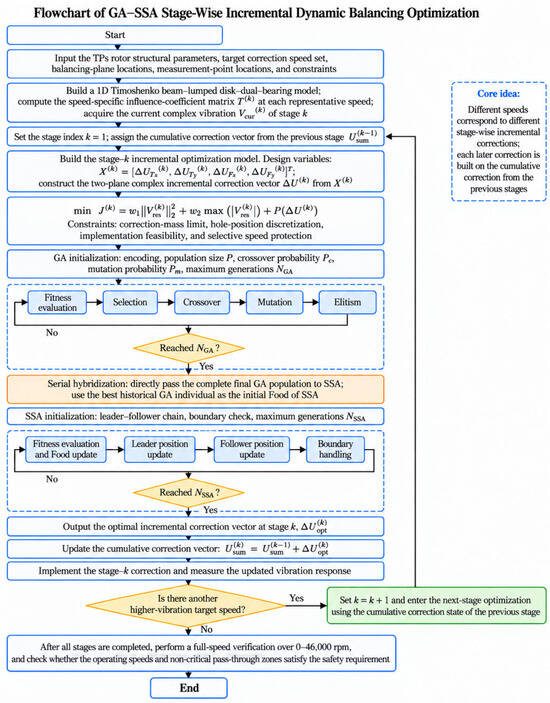
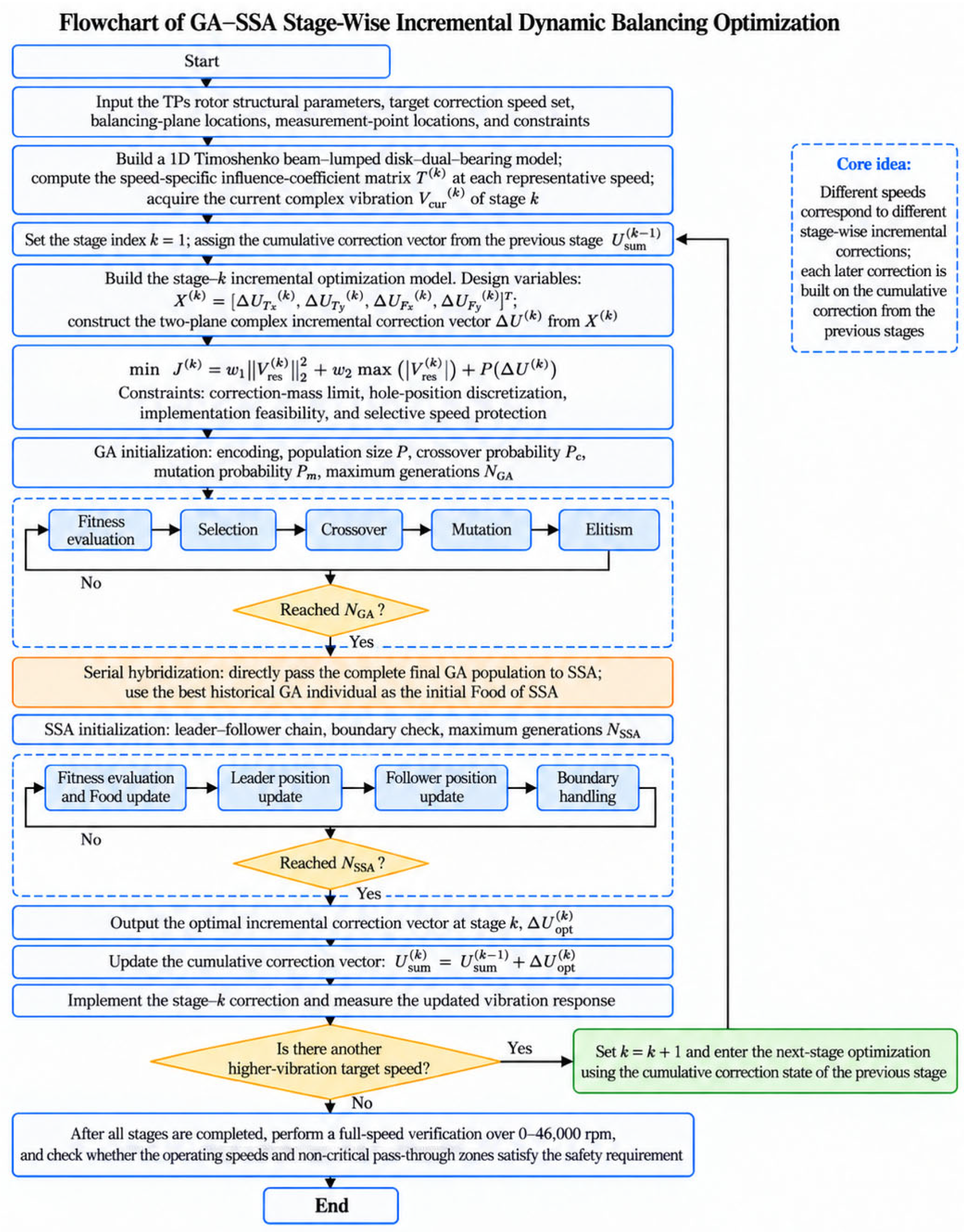
4.5. Serial GA–SSA Procedure and Engineering Output

• Input ${\mathrm{\Omega }}_k$, $V_{cur}^{(k)}$, $T^{\left(k\right)}$, $P_k$, $R_{\lim }$, $R_{safe}$, and $U_{\max }$ for stage $k$, together with the balancing-hole/mass rules and algorithm parameters.
• Generate the initial GA population using the specified random seed, evaluate $J_k$ for all individuals, and establish the historical best solution.
• Execute GA in the sequence “tournament selection–arithmetic crossover–Gaussian mutation–elitist retention–bound correction” until $B_{GA}^{hyb}$ is exhausted.
• Transfer all P individuals from the final GA generation directly as the initial SSA population, and set $X_{best}^{GA}$ as $Food$.
• Update the SSA leader and followers according to Equations (55)–(57), perform bound correction, $J_k$ evaluation, and $Food$ updating, and continue until $B_{SSA}^{hyb}$ is exhausted.
• Convert the final Food back into $\left|\Delta U_n\right|$, ${\alpha }_n$, and the continuous correction mass $\Delta m_n$ for each balancing plane.
• Discretize the balancing-hole position and mass according to Equations (46) and (47), and re-enumerate implementable candidate schemes in the neighborhood of the continuous solution.
• Output the optimal incremental correction scheme $\Delta U^{(k)\ast }$ that satisfies the current vibration limits, the safety constraints at priority-protected speeds, and the installation constraints.

The complete procedure is shown in Figure 1.

Figure 1. Flowchart of GA-SSA Stage-Wise Incremental Dynamic Balancing Optimization.

5. Three-Dimensional Finite Element Model and Dynamic Validation

5.1. Three-Dimensional Finite Element Model and Parameter Settings

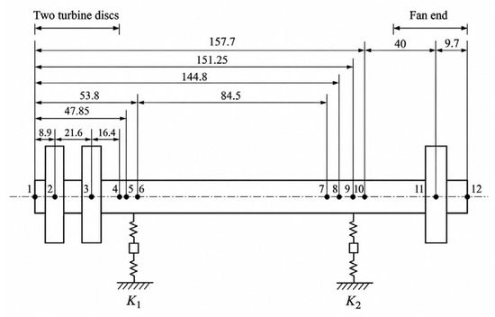
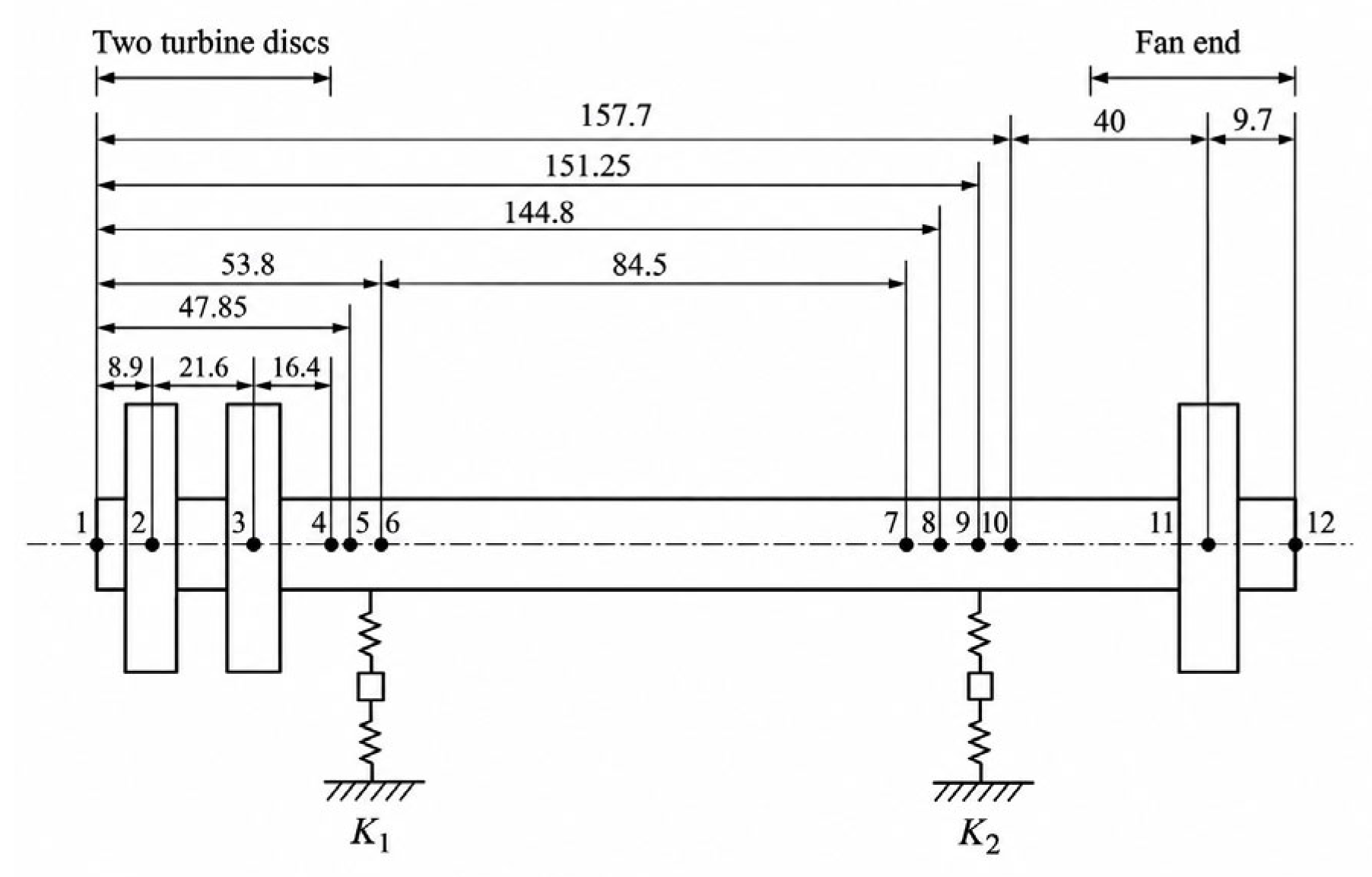
The TPS rotor consists of a two-stage turbine, main shaft, two rolling bearings, and a fan, with the two turbine stages and the fan located outboard of the bearings on opposite sides. Figure 2 shows the principal axial locations, and Table 1 lists the material parameters. These provide a unified structural reference for the one-dimensional model, the three-dimensional model, and the on-site measurement points.

Figure 2. Schematic of the TPS rotor system and main axial locations. Numbers 1–12 denote the axial nodes of the one-dimensional rotor model, and the dashed line represents the rotor centerline (shaft axis). $k_1$ and $k_2$ denote the equivalent bearing supports. All dimensions are in mm.

Table 1. Material properties of the component elements.

Material	E/GPa	G/GPa	β/kg·m−3	ν	Component
GH4169	204	79	8240	0.30	Shaft, flow-guiding cone
TC4	110	43	4510	0.34	Turbine
TC17	112	45	4682	0.33	Fan
304	193	77	7930	0.28	Other components

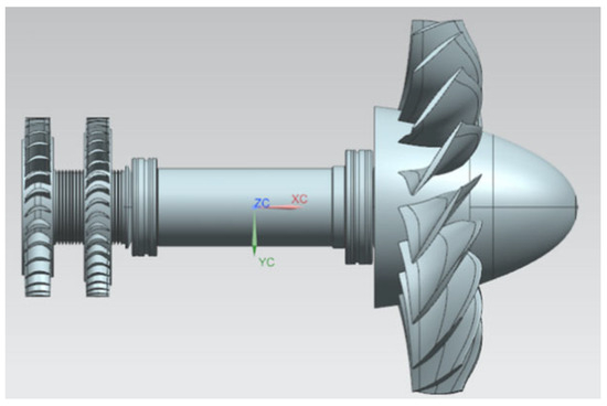
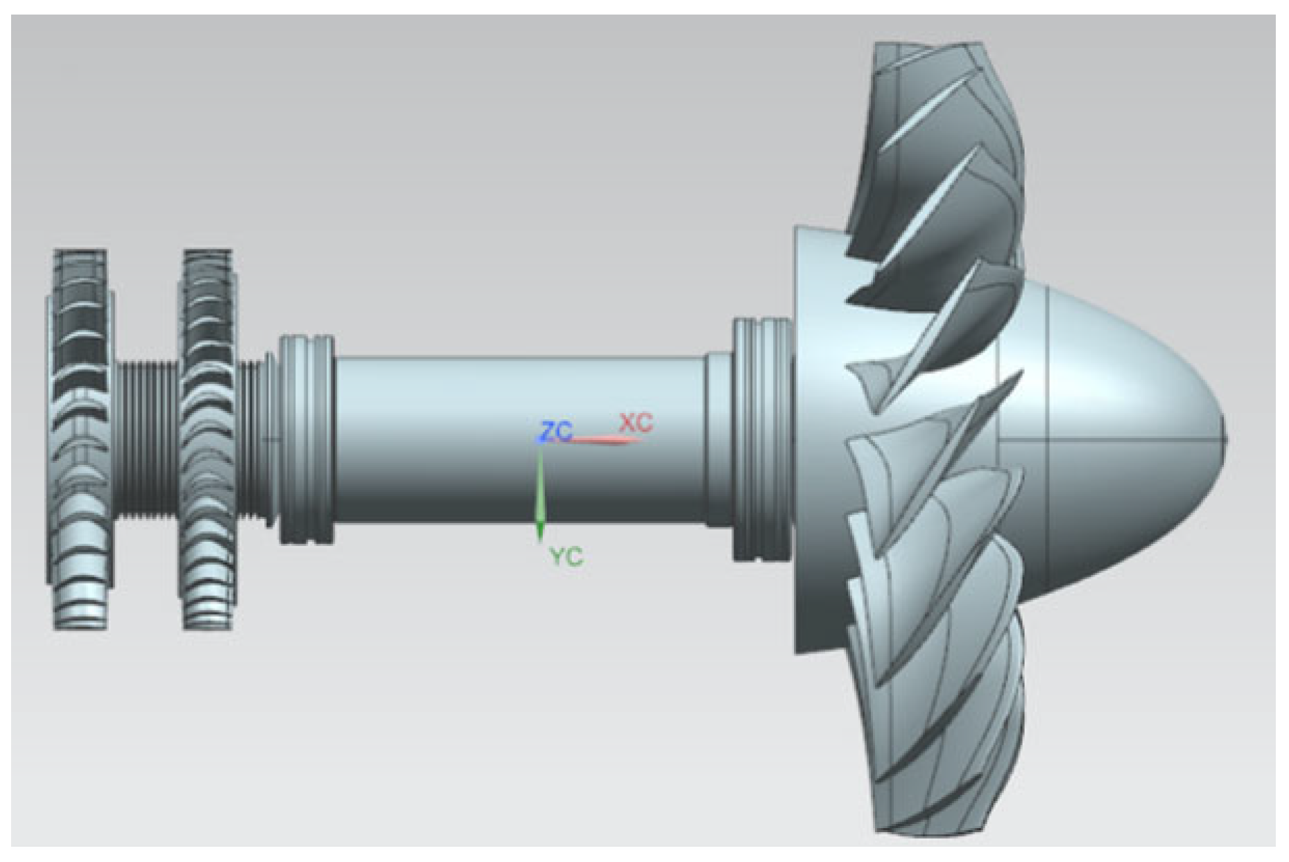
The three-dimensional model was created in Siemens NX 10.0 and imported into ANSYS 2022 R2, as shown in Figure 3. The shaft steps, two turbine stages, fan, disk–shaft connections, and bearing supports were retained, whereas threads and small chamfers were omitted. The rolling bearings were represented by equivalent stiffness–damping supports. The principal finite element settings are listed in Table 2.

Figure 3. Three-dimensional geometric model of the TPS rotor.

Table 2. Principal settings of the three-dimensional finite element model.

Item	Model Setting
Solid/connection element	Linear tetrahedral/wedge SOLID185; bonded contact
Number of elements/nodes	434,147 solid mesh elements/115,680 nodes
Disk–shaft connection	Bonded contact
Bearing support	$K_b$, $C_b$ equivalent support
Structural damping	Rayleigh damping
Gyroscopic effect	Rotational gyroscopic/Coriolis terms included
Harmonic-response excitation	U = 1 g·mm → F = 10−6 UΩ2 N

5.2. Mesh Convergence

Four progressively refined finite element meshes, M1–M4, were established. The four models used identical geometry, materials, supports, connections, and rotational-speed settings; only the global mesh size was varied, while the same local refinement was applied near abrupt shaft-diameter changes, disk–shaft connections, and bearing supports [39]. The mesh parameters are listed in Table 3. Mesh convergence was evaluated using the first lateral bending natural frequency in the stationary state, which was converted to an equivalent rotational speed as

$$n_{eq,1}=60f_1$$

(58)

where $f_1$ is the first lateral bending natural frequency in the stationary state and $n_{eq,1}$ is the corresponding equivalent rotational speed. This quantity is used only for comparing mesh convergence and does not represent the actual critical speed when gyroscopic effects are included.

Table 3. Mesh models and equivalent rotational speeds corresponding to the first lateral bending natural frequency.

Mesh	Global/mm	Local/mm	Mechanical Nodes	Solid Mesh Elements	Total Solver Elements	Eq. Speed/rpm
M1	5.0	1.5	94,150	358,450	405,186	11,463.95
M2	4.0	1.5	99,312	375,856	428,533	11,297.86
M3	3.2	1.5	107,483	405,411	464,067	11,403.36
M4	2.7	1.5	115,680	434,147	501,121	11,377.76

The relative change between two adjacent meshes is defined as

$${\epsilon }_n=\left|n_{eq,1}^{(b)}-n_{eq,1}^{(a)}\right|÷n_{eq,1}^{(b)}\times 100\%$$

(59)

where $a$ and $b$ denote the coarser and finer meshes, respectively.

As shown in Table 3, the equivalent rotational speeds for M1–M4 are 11,463.95, 11,297.86, 11,403.36, and 11,377.76 rpm, respectively. The difference between M3 and M4 is only 25.60 rpm, corresponding to a relative change of approximately 0.23%, indicating that further mesh refinement has little effect on the overall modal results. Therefore, the M4 mesh is used for the subsequent Campbell diagram, rotating modal analysis, and harmonic-response calculations.

5.3. Rotating Modal Characteristics and Baseline Response Validation

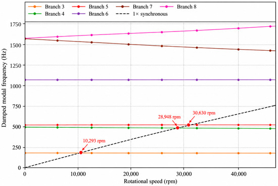
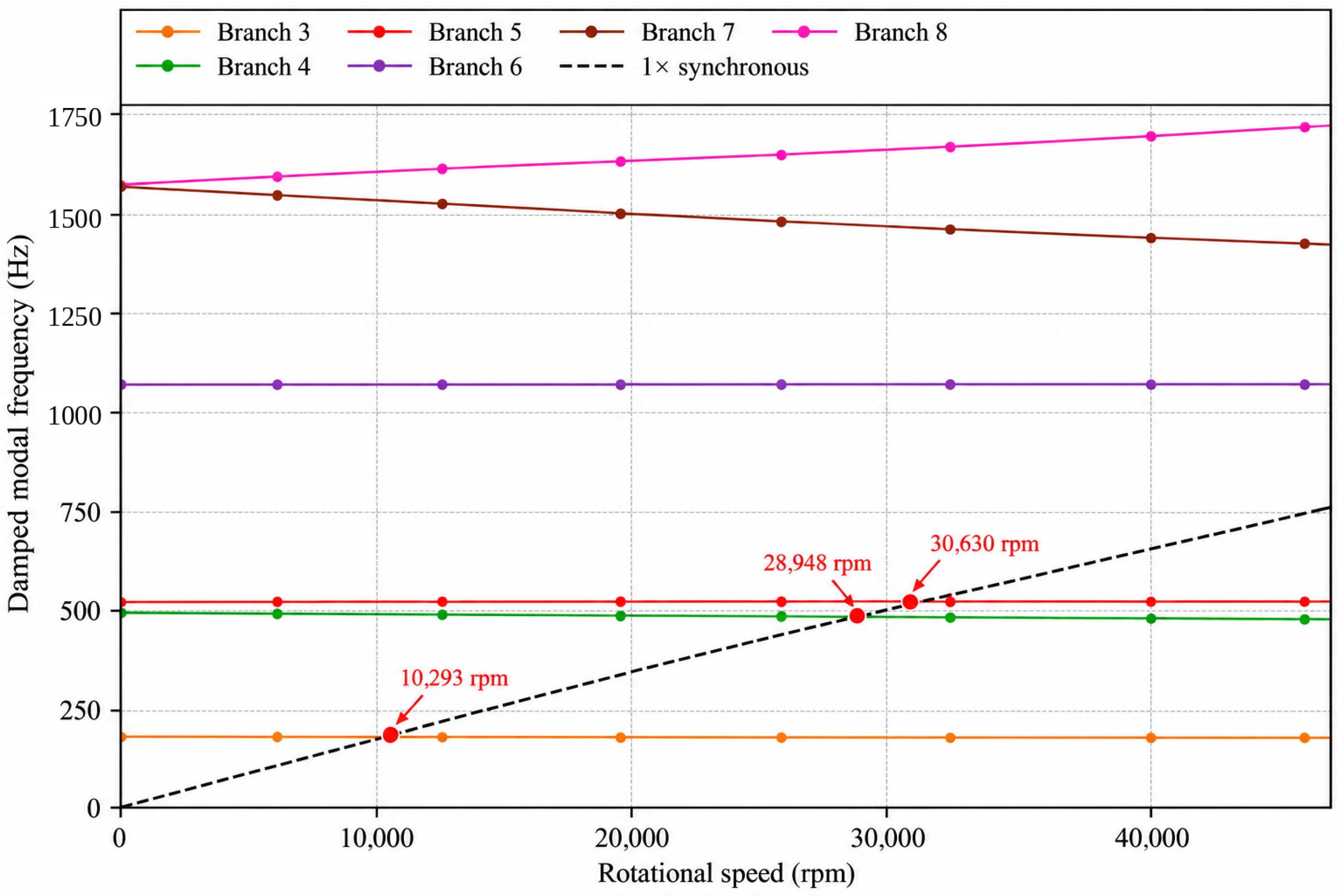
Gyroscopic effects were included in the M4 model, and the Campbell diagram was calculated over 0–46,000 rpm (Figure 4). Mass unbalance generates synchronous 1× excitation at a frequency of n/60, and the intersections between the synchronous line and the rotating modal branches were used to determine the principal critical speeds.

Figure 4. Campbell diagram of the TPS rotor system over 0–46,000 rpm.

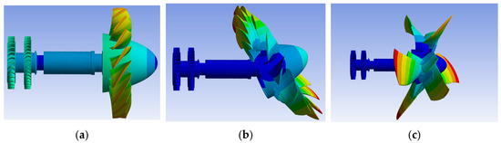
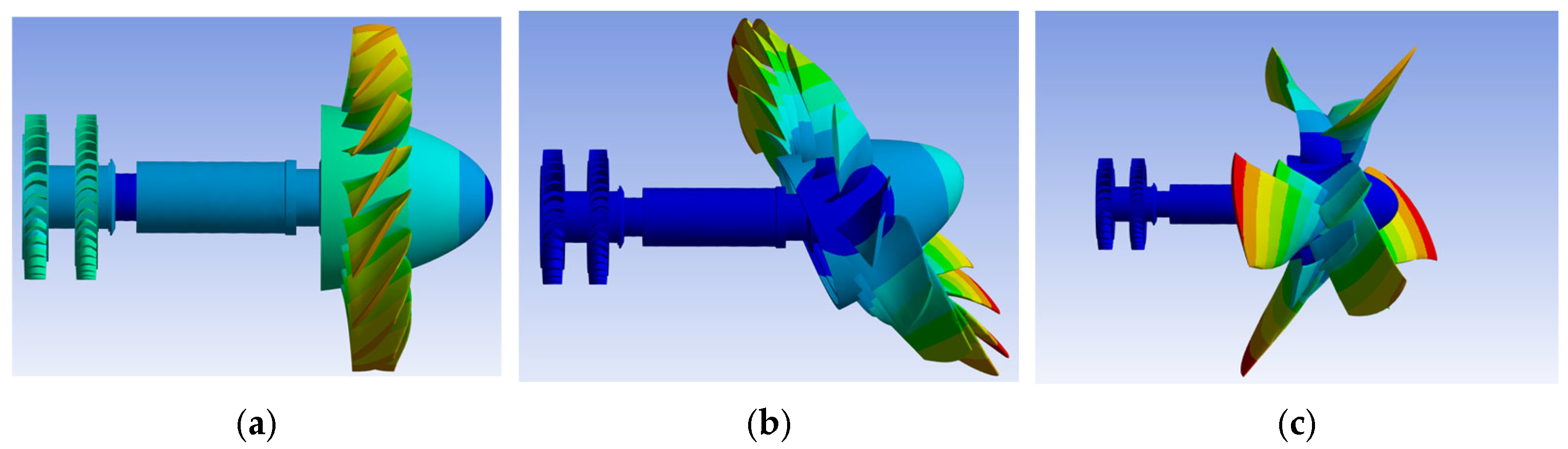
The first three principal critical speeds indicated in Figure 4 are approximately 10,293, 28,948, and 30,630 rpm, with the corresponding mode shapes shown in Figure 5. Table 4 further compares the results from the one-dimensional model, the 3D ANSYS model, and experimental identification.

Figure 5. First three principal bending mode shapes of the TPS rotor. (a) First mode; (b) second mode; (c) third mode. The colors indicate the relative magnitude of the modal deformation and do not represent the actual vibration displacement amplitude.

Table 4. Comparison of the first three critical speeds.

Order	1D Model/rpm	3D ANSYS/rpm	Experiment/rpm	3D ANSYS–Experiment Error/%
1st	11,750	10,293	11,038	6.75
2nd	27,250	28,948	27,014	7.16
3rd	33,430	30,630	33,586	8.80

The value of 11,377.76 rpm in Table 3 is the equivalent rotational speed corresponding to the first lateral natural frequency in the stationary state, whereas 10,293 rpm in Figure 4 is the synchronous critical speed obtained with gyroscopic effects included. These two quantities have different physical meanings; the latter is taken as the actual critical speed.

The relative errors of the 3D ANSYS predictions for the first three critical speeds are 6.75%, 7.16%, and 8.80%, respectively. The modal order and overall trend are consistent with the experimental results, indicating that the model captures the principal rotating modal characteristics of the TPS rotor.

The first critical speed of 10,293 rpm is close to the first balancing stage at 10,358 rpm; therefore, this stage lies in a speed-up-sensitive region. The purpose of balancing at this point is to reduce synchronous vibration while passing through the first critical-speed region, rather than to operate continuously near the critical speed.

To further validate the amplitude-and-phase prediction capability required for the subsequent complex influence coefficients, three representative speeds, 10,358, 25,558, and 38,333 rpm, were selected, and the 1× vibration amplitudes and phases obtained from ANSYS were compared with the experimental results.

The relative error of vibration amplitude is defined as

$${\epsilon }_n=\left|\begin{array}{c}{A}_{ANSYS}-A_{\exp }\end{array}\right|÷A_{\exp }\times 100\%$$

(60)

The phase error is defined as the minimum angular difference under the periodic phase convention:

$${\Delta }_{\varphi }=\min \left[\left|{\varphi }_{ANSYS}-{\varphi }_{\exp }\right|,360°-\left|{\varphi }_{ANSYS}-{\varphi }_{\exp }\right|\right]$$

(61)

The comparison results are presented in Table 5.

Table 5. Comparison of baseline amplitude and phase between the three-dimensional model and experiments at representative speeds.

Speed/rpm	Point	Exp. Amp./(mm/s)	Exp. Phase/°	ANSYS Amp.	ANSYS Phase/°	Amp. Error/%	Phase Error/°
10,358	Turbine end	3.10	213.3	2.80	210.1	9.7	3.2
10,358	Fan end	2.87	263.4	2.75	259.5	4.2	3.9
25,558	Turbine end	1.18	297.6	1.09	301.4	7.6	3.8
25,558	Fan end	5.04	317.8	5.11	313.7	1.4	4.1
38,333	Turbine end	2.62	321.7	2.80	321.5	6.9	0.2
38,333	Fan end	2.37	331.3	2.16	338.4	8.9	7.1

All six amplitude errors in Table 5 are below 10%, and the phase errors do not exceed 7.1°, indicating that the M4 model can adequately describe the complex 1× vibration at the representative speeds and can therefore be used to extract influence coefficients.

5.4. Extraction and Application of Speed-Specific Influence Coefficients

The validated M4 model was used to extract speed-specific influence coefficients at three representative speeds: 10,500, 25,500, and 38,000 rpm.

At each speed, a unit complex unbalance of 1 g·mm was applied separately at the two balancing planes and converted into an SI harmonic excitation according to the synchronous centrifugal-force relationship. By extracting the complex 1× vibration velocities at the turbine and fan ends, the influence coefficients corresponding to balancing plane 1 are obtained as

$$\begin{array}{cc}{T}_{11}^{\left(k\right)}={\displaystyle \frac{V_1^{\left(k\right)}}{U_1^{\left(k\right)}}},& T_{21}^{\left(k\right)}={\displaystyle \frac{V_2^{\left(k\right)}}{U_1^{\left(k\right)}}}\end{array}$$

The same procedure is used for balancing plane 2 to obtain

$$\begin{array}{cc}{T}_{12}^{\left(k\right)}={\displaystyle \frac{V_1^{\left(k\right)}}{U_2^{\left(k\right)}}},& T_{22}^{\left(k\right)}={\displaystyle \frac{V_2^{\left(k\right)}}{U_2^{\left(k\right)}}}\end{array}$$

At the $k$th representative speed, the influence coefficient matrix is

$$T^{\left(k\right)}=\left[\begin{array}{cc}{T}_{11}^{\left(k\right)}& T_{12}^{\left(k\right)}\\ T_{21}^{\left(k\right)}& T_{22}^{\left(k\right)}\end{array}\right]$$

Its unit is (mm/s)/(g.mm)

Table 6 lists the complex influence coefficients at the three representative speeds. The rows correspond to the two measurement points, the columns correspond to the two balancing planes, and each element is expressed in the form “magnitude ∠ phase”.

Table 6. Speed-specific influence coefficient matrices at three representative speeds.

Speed/rpm	T11	T12	T21	T22
10,500	0.619 ∠ 4.046°	0.558 ∠ 33.332°	0.736 ∠ 11.137°	0.548 ∠ 7.395°
25,500	5.090 ∠ 276.393°	10.142 ∠ 83.252°	1.641 ∠ 303.699°	2.661 ∠ 283.111°
38,000	2.002 ∠ 74.376°	15.045 ∠ 273.466°	3.094 ∠ 285.472°	1.112 ∠ 298.110°

Table 6 shows that the influence coefficients vary markedly with rotational speed. Therefore, each balancing stage uses T(k) corresponding to its own speed rather than a single fixed coefficient matrix for all speeds. The currently measured complex vibration and T(k) are substituted jointly into Equation (29) as the direct inputs for GA–SSA to determine the incremental correction.

6. GA–SSA Search Performance and Statistical Analysis

Section 4 provides the dynamic inputs for the representative stages. In this section, the measured vibration, influence coefficients, variable bounds, objective function, and constraints are fixed, and only the search algorithms are compared.

6.1. Comparison Algorithms and Unified Evaluation Conditions

GA, SSA, and PSO were selected as comparison algorithms. All four algorithms used the same population size, function-evaluation budget, and 30 paired random seeds, as listed in Table 7. Because different algorithms may invoke the objective function a different number of times per generation, computational effort was measured uniformly using function evaluations [40]. GA–SSA contains only the two serial stages, GA and SSA; no Nelder–Mead search, multicenter search, or dual-start refinement was used, and all objective-function calls were included in the total budget.

Table 7. Unified computational settings for the comparison algorithms.

Parameter	GA	SSA	PSO	GA–SSA
Population size P	60	60	60	60
Total function-evaluation budget	12,060	12,060	12,060	12,060
GA generations	200	—	—	180
SSA generations	—	200	—	20
PSO iterations	—	—	200	—
Crossover probability $P_c$	0.85	—	—	0.85 (GA stage)
Mutation probability $P_m$	0.18	—	—	0.18 (GA stage)
Independent paired runs	30	30	30	30
Random seeds IDs	51–80	51–80	51–80	51–80

The total function-evaluation budget for all four algorithms was 12,060, and the random seeds IDs were uniformly set to 51–80 to reduce the influence of computational budget and initial randomness on the comparison.

6.2. Convergence and Repeatability Statistics

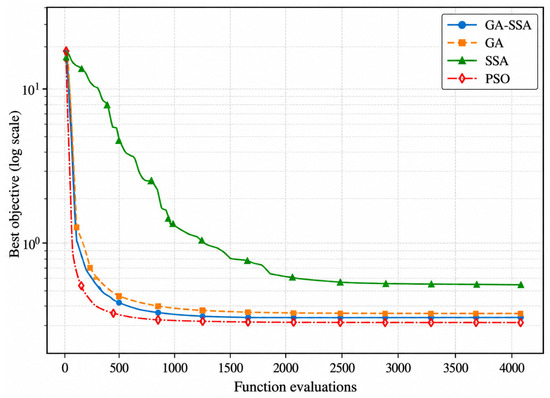
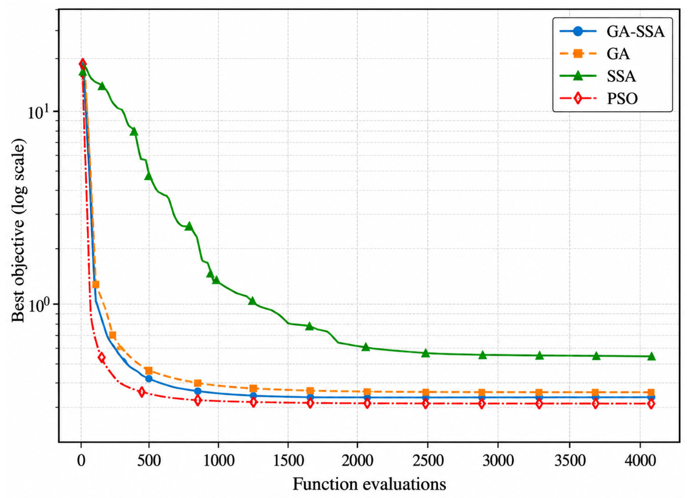
Representative convergence processes of the four algorithms are shown in Figure 6. The horizontal axis denotes the number of function evaluations, and the vertical axis denotes the current best objective-function value; a smaller objective value indicates a better overall optimization result.

Figure 6. Best-objective convergence histories of the four algorithms in representative independent runs.

As shown in Figure 6, GA, PSO, and GA–SSA all enter the low-objective-value region relatively quickly, whereas SSA decreases more slowly. GA–SSA first uses GA to form a higher-quality candidate population and then continues the search with SSA, thereby avoiding the prolonged residence of standalone SSA in a high-objective-value region during the early search stage.

A single convergence curve cannot represent the overall performance of a stochastic algorithm. Therefore, Mean, SD, Median, IQR, Bootstrap 95% CI, Best, and Worst were further calculated for the 30 paired runs, with the results listed in Table 8.

Table 8. Statistical results from 30 paired independent runs of the four algorithms.

Alg	Mean	SD	Median	IQR	Bootstrap 95% CI	Best	Worst
GA	0.352	0.186	0.301	0.042	[0.307, 0.425]	0.286	1.29
SSA	6.2	6.79	4.27	4.2	[4.06, 8.73]	0.313	28.8
PSO	0.285	1.95 × 10−5	0.285	9.90 × 10−6	[0.285110, 0.285123]	0.285105	0.285208
GA–SSA	0.351	0.156	0.303	0.043	[0.308, 0.412]	0.286	1.11

Table 8 shows that PSO has the lowest mean objective-function value (0.285) and the smallest SD and IQR, indicating the best repeatability for this representative numerical problem. The Mean of GA–SSA is 0.351, close to the GA value of 0.352; its SD decreases from 0.186 to 0.156 and its Worst value decreases from 1.29 to 1.11. Thus, the serial hybridization changes the average performance only slightly but reduces the variability in some repeated runs.

For standalone SSA, the Mean, SD, IQR, and Worst values increase markedly. By contrast, GA–SSA does not exhibit such wide dispersion, indicating that initializing SSA with the final GA population improves the search stability of standalone SSA in the current constrained space.

Therefore, the principal performance characteristic of GA–SSA is that it maintains an overall search level comparable to GA while reducing variability in some runs and substantially improving standalone SSA, rather than achieving the best result for every statistical metric.

6.3. Paired Statistical Tests

To determine whether the observed differences are statistically significant, two-sided Wilcoxon signed-rank tests were conducted using the 30 paired random seeds, and the Holm method was applied to correct for multiple comparisons. The results are listed in Table 9.

Table 9. Paired statistical tests of GA–SSA against the comparison algorithms.

Comparison	Statistical Test	Raw p	Holm-Adjusted p	Rank-Biserial rrb
GA–SSA vs. GA	Paired Wilcoxon	0.0577	0.0577	−0.398
GA–SSA vs. SSA	Paired Wilcoxon	2.61 × 10−8	5.22 × 10−8	0.974
GA–SSA vs. PSO	Paired Wilcoxon	1.86 × 10−9	5.59 × 10−9	−1.00

For GA–SSA versus GA, the Holm-adjusted p value is 0.0577, and the difference does not reach the 0.05 significance level. The difference between GA–SSA and standalone SSA is significant and favors GA–SSA. A significant difference is also observed between GA–SSA and PSO; however, PSO yields lower and more stable objective-function values for this numerical problem. These findings are consistent with the statistical distributions in Table 8.

Accordingly, GA–SSA does not have an absolute numerical advantage over all comparison algorithms. Its role in this study is to embed the early-stage population search of GA and the later-stage SSA updates into the staged incremental balancing procedure, thereby producing two-plane corrections that satisfy practical balancing constraints. Its engineering performance is further evaluated through on-site tests in Section 6.

7. Results of the Staged Incremental On-Site Dynamic Balancing Tests

7.1. On-Site Dynamic Balancing Test System

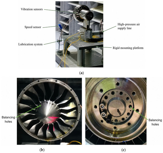
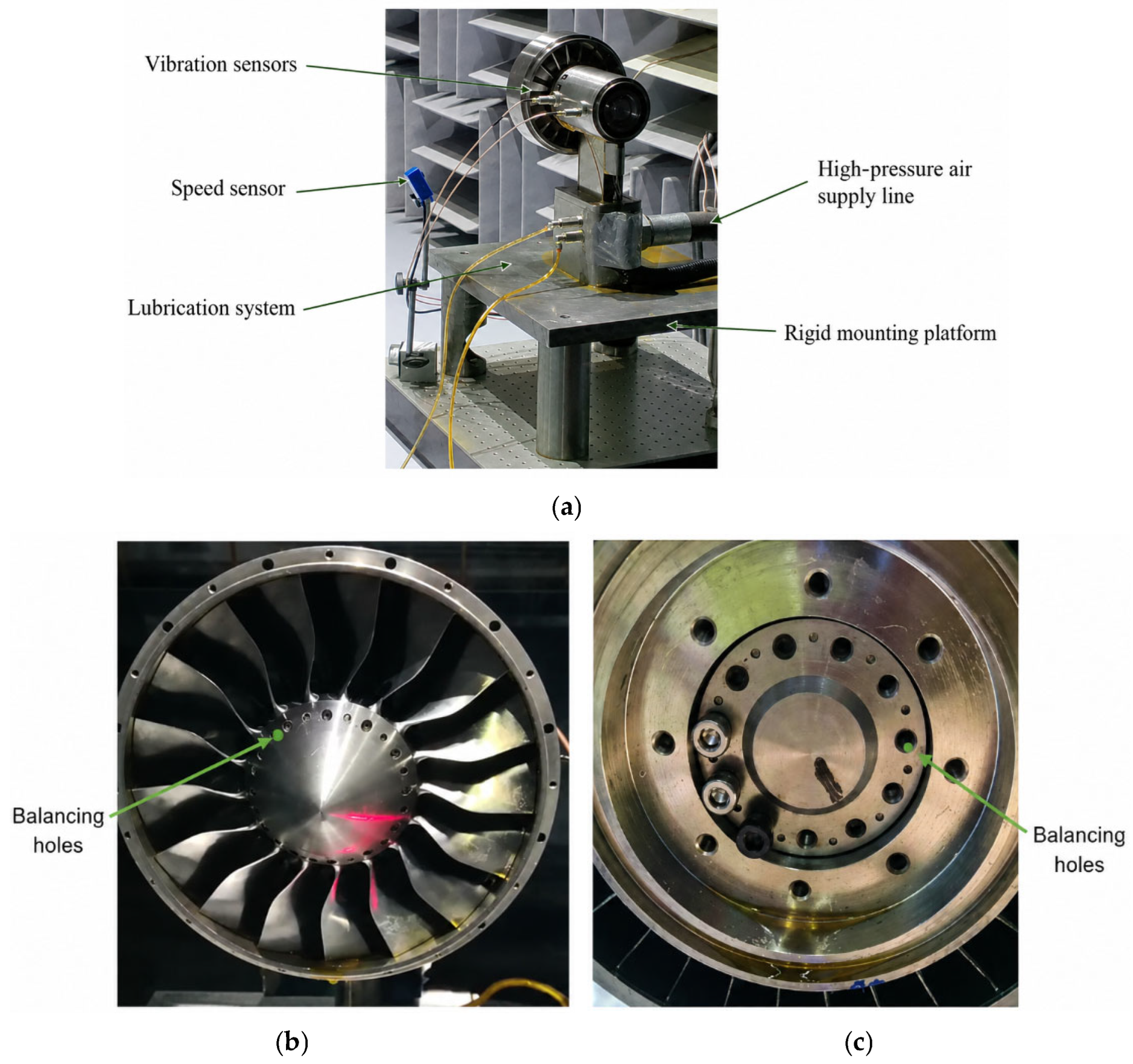
The on-site test system is shown in Figure 7 and includes the TPS test article, vibration measurement points at both rotor ends, a rotational-speed monitoring location, and two balancing planes, a lubrication system, a high-pressure air supply system, and a rigid mounting platform. The TPS test article, rigid mounting platform, and data acquisition system were independently developed and integrated by Changchun University of Science and Technology (Changchun, China). The lubrication system was an O1/04/70/dz1/S7/G1 oil-air lubrication unit (REBS Lubrication Echnology Ltd., Shanghai, China), while the high-pressure air was supplied by the facility of AVIC Aerodynamics Research Institute (Harbin, China). The vibration signals were measured using G100 vibration sensors (Shanghai Guanjin Instrument Co., Ltd., Shanghai, China), and the rotational speed was measured using an ROS-P remote optical sensor (Monarch Instrument, Amherst, NH, USA). The signals were synchronously acquired using the self-developed data acquisition system equipped with an NI-9232 acquisition module (National Instruments, Austin, TX, USA). The principal sensor parameters are listed in Table 10. During the tests, rotational speed and the amplitude and phase of the 1× vibration at both ends were recorded synchronously. A common phase-zero reference, rotation direction, and measurement-point definition were used to ensure consistency with the model-based influence coefficients.

Figure 7. Layout of the TPS on-site dynamic balancing test system: (a) on-site dynamic balancing test system; (b) fan-end balancing position; (c) turbine-end balancing position.

Table 10. Principal parameters and uncertainties of the test measurement chain.

Item	Model	Range/Sensitivity	Frequency Range/Bandwidth	Calibration and Uncertainty
Turbine-end vibration sensor	G100	20 (mV/mm/s)	10–1000 Hz	U ≈ 0.29 mm/s
Fan-end vibration sensor	G100	20 (mV/mm/s)	10–1000 Hz	U ≈ 0.29 mm/s
Rotational-speed sensor	ROS-P	1–250,000 rpm	0.0167–4166.7 Hz	±0.0015%
Data acquisition module	NI-9232	102.4 kS/s/channel	0.985–102.4 kS/s	0.1 Hz (−3 dB)

The on-site validation was conducted in two steps. First, the amplitudes and phases before and after balancing were compared at the three representative stages. Second, the final cumulative correction state was verified over the full speed range of 0–46,000 rpm.

7.2. Staged Correction Results at Representative Speeds

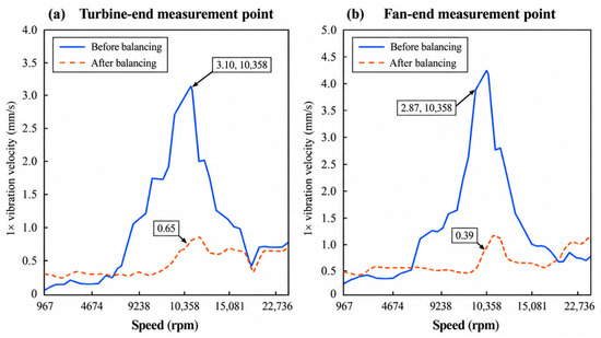
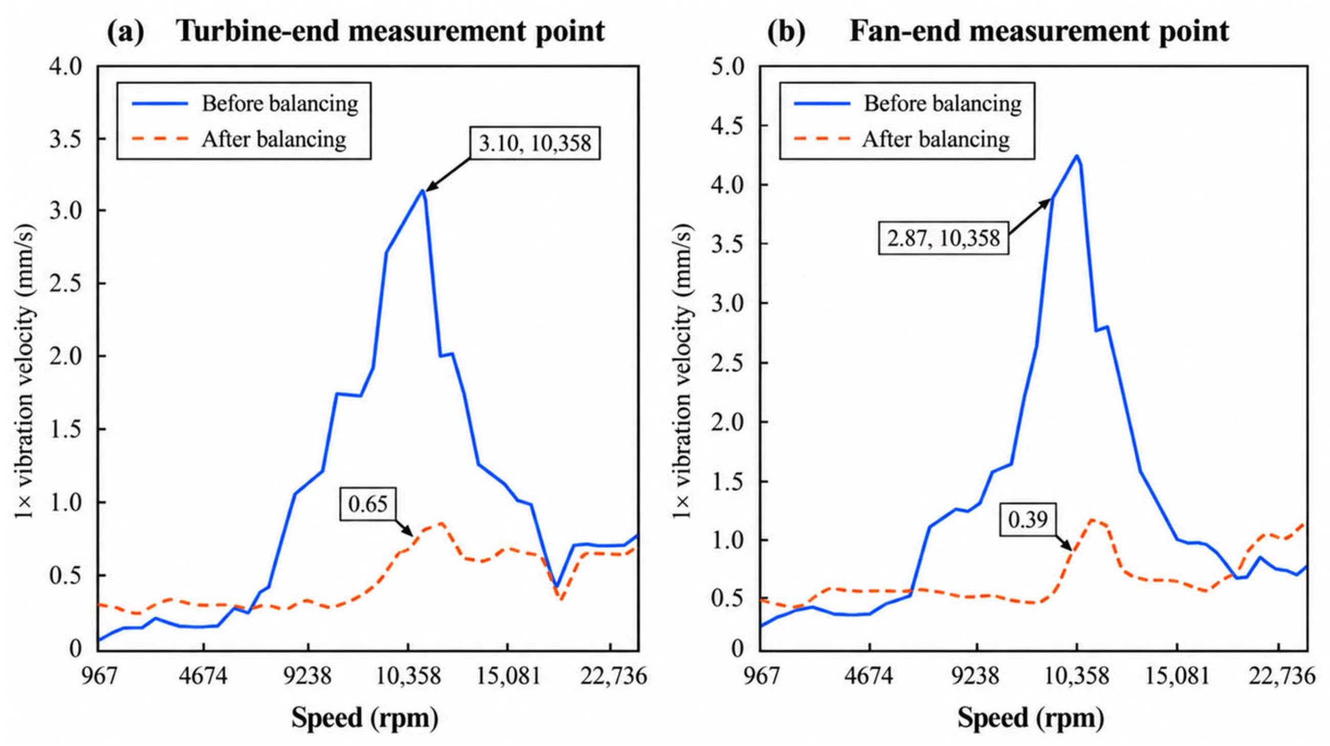
The speeds of 10,358, 25,558, and 38,333 rpm are three representative stages treated sequentially during acceleration. At each stage, the existing balancing weights were retained, and a new incremental correction was calculated from the currently measured vibration. Table 11 summarizes the amplitudes and phases at both rotor ends, while Figure 8, Figure 9 and Figure 10 present the corresponding velocity responses.

Table 11. Vibration amplitude and phase before and after balancing at the three representative stages.

Stage	Turbine End Before Balancing	Turbine End After Balancing	Fan End Before Balancing	Fan End After Balancing
10,358 rpm	3.10 mm/s ∠ 213.3°	0.65 mm/s ∠ 265.7°	2.87 mm/s ∠ 263.4°	0.39 mm/s ∠305.8°
25,558 rpm	1.18 mm/s ∠ 297.6°	0.20 mm/s ∠260.5°	5.04 mm/s ∠ 317.8°	0.85 mm/s ∠295.6°
38,333 rpm	2.62 mm/s ∠ 321.7°	0.43 mm/s ∠ 250.8°	2.37 mm/s ∠ 331.3°	0.42 mm/s ∠ 164.5°

Figure 8. Change in 1× vibration velocity before and after balancing at the 10,358 rpm stage.

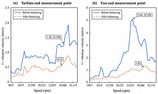
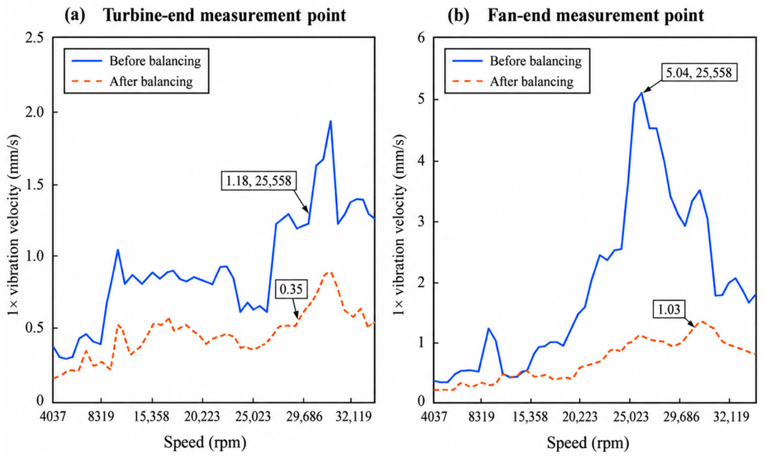
Figure 9. Change in 1× vibration velocity before and after balancing at the 25,558 rpm stage.

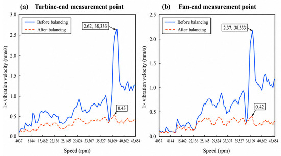
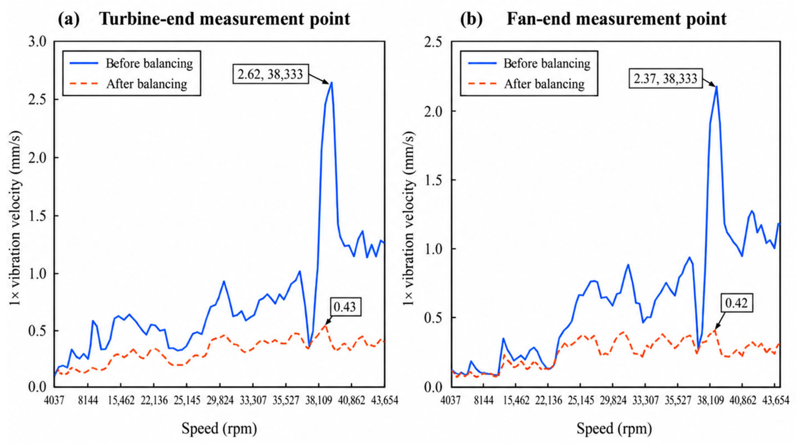
Figure 10. Change in 1× vibration velocity before and after balancing at the 38,333 rpm stage.

The 1× vibration at both rotor ends decreases markedly at all three stages, with reductions of 79.0–86.4%.

7.2.1. Stage near the First Critical Speed (10,358 rpm)

The speed of 10,358 rpm lies within the neighborhood of the first critical speed. After the incremental correction, the turbine-end vibration velocity decreases from 3.10 to 0.65 mm/s, while the fan-end value decreases from 2.87 to 0.39 mm/s. The corresponding velocity response is shown in Figure 8.

Figure 8 shows that the principal peak in the critical-speed neighborhood is substantially reduced. The first-stage correction therefore provides a more stable vibration state for further acceleration.

7.2.2. Medium-to-High-Speed Stage (25,558 rpm)

After retaining the cumulative correction from the first stage, the rotor was accelerated to 25,558 rpm, where relatively high 1× vibration appeared at the fan end. Following the second-stage correction, the turbine-end vibration velocity decreased from 1.18 to 0.20 mm/s, and the fan-end value decreased from 5.04 to 0.85 mm/s, as shown in Figure 9.

Figure 9 shows a pronounced reduction in the dominant fan-end peak, accompanied by a simultaneous decrease at the turbine end. This indicates that the combined two-plane correction can be readjusted for the current stage while retaining the corrections applied at previous stages.

7.2.3. High-Speed Stage (38,333 rpm)

The third-stage correction was implemented after further acceleration to 38,333 rpm. The turbine-end vibration velocity decreases from 2.62 to 0.43 mm/s, and the fan-end value decreases from 2.37 to 0.42 mm/s, corresponding to reductions of 83.6% and 82.3%, respectively, as shown in Figure 10.

Figure 10 shows that the principal vibration peak at the high-speed stage is likewise suppressed. Together, the three stages demonstrate the procedure of retaining the cumulative balancing correction and continuing with incremental correction according to the current state. The final operating condition must still be assessed through full-speed-range verification.

7.3. Full-Speed-Range Verification Under the Final Cumulative Correction State

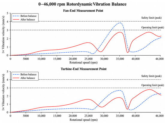
After completing the corrections at all stages, the rotor was accelerated again from 0 to 46,000 rpm under the final cumulative correction state, while the 1× vibration at both ends was recorded continuously. Figure 11 presents the final vibration response throughout the complete acceleration process.

Figure 11. Full-speed-range vibration verification under the final cumulative correction state.

Although local peaks remain in the resonance-sensitive regions in Figure 11, the target operating speeds and the principal noncritical acceleration intervals remain within the specified limits. This indicates that the final cumulative balancing correction satisfies the overall acceleration and operating requirements.

8. Discussion

The staged incremental method differs from approaches that determine a common correction in a single step. Each stage starts from the current cumulative correction and the measured complex vibration, determines only the incremental correction for that stage, and then proceeds to a higher speed. Because a later-stage correction may alter the vibration at some previously treated speeds, the final evaluation in this study is based on whether the target operating speeds and the entire acceleration process satisfy the prescribed operating requirements.

The three-dimensional finite element model serves two purposes: validating the principal dynamic characteristics of the TPS rotor and providing speed-specific influence coefficients. The equivalent rotational speed corresponding to the first lateral natural frequency changes by approximately 0.23% from M3 to M4; the errors between the first three critical speeds and the experimental values are 6.75–8.80%; and, at representative speeds, the amplitude error is below 10%, and the phase error does not exceed 7.1%. These results support the use of the M4 model for influence-coefficient extraction, although bearing stiffness, damping, and connection parameters can still affect prediction accuracy.

The algorithm comparison shows that GA–SSA has an overall search level comparable to GA, while its SD and Worst values are lower than those of GA, and the stability of standalone SSA is markedly improved. PSO achieves lower and more stable objective-function values for the fixed numerical problem. Therefore, the value of GA–SSA does not lie in universally outperforming all optimizers, but in its ability to be embedded in the staged incremental balancing procedure and to produce stable, constrained, and implementable corrections.

At all three representative on-site stages, the 1× vibration at both rotor ends is substantially reduced, indicating that the sequence “dynamic model–speed-specific influence coefficients–GA–SSA search–engineering discretization–on-site implementation” forms an effective closed loop. For on-site dynamic balancing, implementable corrections and the final vibration-reduction performance are as important as the ranking of a single objective-function value.

This study still has several limitations. The bearings are represented by operating-point linear stiffness–damping models, without explicitly accounting for preload, temperature, lubrication, or speed-dependent support parameters. In addition, on-site corrections were implemented only at representative high-vibration stages. Future work may incorporate speed-dependent bearing parameters, thermo-structural coupling, and online model updating to improve the prediction accuracy of influence coefficients and correction quantities at high speeds.

9. Conclusions

To address high 1× vibration during the staged speed-up of a TPS rotor, this study establishes a dynamic model, a staged incremental balancing model, and a serial GA–SSA optimization method, and validates them through finite element analysis and on-site tests. The main conclusions are as follows.

(1)

The one-dimensional Timoshenko-beam–lumped-disk–dual-bearing model and the three-dimensional ANSYS model can capture the principal dynamic characteristics of the TPS rotor. The equivalent rotational speed corresponding to the first lateral natural frequency changes by approximately 0.23% from meshes M3 to M4. The errors in the first three critical speeds relative to the experimental results are 6.75%, 7.16%, and 8.80%, respectively. At representative speeds, the amplitude error is below 10%, and the phase error does not exceed 7.1%, supporting the extraction of speed-specific influence coefficients.

(2)

The staged incremental model starts from the currently measured complex vibration and the cumulative balancing correction, and only the two-plane incremental correction for the current stage is determined at each step. Subsequent corrections are allowed to alter the local response at some historical speeds, while the cumulative correction effect is ultimately evaluated through the full-speed-range acceleration response.

(3)

GA–SSA transfers the complete final GA population to SSA and uses the historical best GA individual as the initial Food. Under the same function-evaluation budget and 30 paired runs, its Mean is close to that of GA, while SD decreases from 0.186 to 0.156 and Worst decreases from 1.29 to 1.11; compared with standalone SSA, search stability is significantly improved. PSO performs better on the fixed numerical problem, indicating that the primary advantage of GA–SSA lies in its integration with the staged incremental balancing constraints and its ability to obtain stable, implementable solutions.

(4)

At the three representative on-site stages, the 1× vibration velocities at both rotor ends are reduced by 79.0–86.4%. In the final verification over 0–46,000 rpm, the target operating speeds and the principal noncritical acceleration intervals remain within the specified limits, demonstrating that the cumulative incremental balancing correction satisfies the overall operating requirements of the TPS.

References

- Zhao, S.; Zheng, M.; Yang, Y.; Cheng, H. The unbalance parameters detection method for pump rotor based on BP neural network. Int. J. Dyn. Control 2026, 14, 139. [Google Scholar] [CrossRef] [Scilit]
- Zhao, J.; Yang, Y.; Deng, W.; Liu, W.; Fu, C.; Zhao, S.; Ren, X.; Nie, Z.; Zhao, Y. The influence of unbalance identification position on the transient dynamic balancing of a single-disk rotor without trial weights. J. Vib. Control, 2025; OnlineFirst. [CrossRef] [Scilit]
- Zhang, X.; Yang, Y.; Deng, W.; Zhao, S.; Zhu, Q.; Ma, H.; Han, Q.; Qin, Z.; Liu, W. Vibration energy analysis of rub-impact rotor system: Nonlinear fault-induced energy response and transfer state. Mech. Syst. Signal Process. 2025, 236, 113035. [Google Scholar] [CrossRef] [Scilit]
- Guan, X.; Peng, H.; Li, H.; Zhang, J. Dynamic Balance Correction of Active Magnetic Bearing Rotor Based on Adaptive Notch Filter and Influence Coefficient Method. Appl. Sci. 2025, 15, 4147. [Google Scholar] [CrossRef] [Scilit]
- Deng, Z.; Wu, T.; Deng, W.; Huang, X.; Wu, D.; Zhang, B.; Luo, H. A resonance-avoiding modal balancing method for multimodal balancing of high-speed flexible rotors. Meas. Sci. Technol. 2025, 36, 016031. [Google Scholar] [CrossRef] [Scilit]
- Xiang, L.; Zhang, X.; Zhang, Y.; Hu, A.; Bing, H. A novel method for rotor fault diagnosis based on deep transfer learning with simulated samples. Measurement 2023, 207, 112350. [Google Scholar] [CrossRef] [Scilit]
- Aroui, T.; Marmouch, S. Improved deep-learning rotor fault diagnosis based on multi vibration sensors and recurrence plots. J. Vib. Control 2025, 31, 1874–1883. [Google Scholar] [CrossRef] [Scilit]
- Ming, A.; Zhang, W.; Fu, C.; Yang, Y.; Chu, F.; Liu, Y. L-kurtosis-based optimal wavelet filtering and its application to fault diagnosis of rolling element bearings. J. Vib. Control 2024, 30, 1594–1603. [Google Scholar] [CrossRef] [Scilit]
- Wang, T.; Ding, Q. Modal balancing for ball bearing-rotor system using nonlinear normal modes. J. Sound Vib. 2023, 547, 117507. [Google Scholar] [CrossRef] [Scilit]
- Wang, Z.; Li, D.; Wang, Z.; Liu, A.; Tao, R. Research on dynamic balance of spindle rotor system based on particle swarm optimization. Adv. Mater. Sci. Eng. 2021, 2021, 9728248. [Google Scholar] [CrossRef] [Scilit]
- Moorthi, L.R.; Inayat-Hussain, J.I.; Zakaria, A.A. Effect of bearing wear on linear and nonlinear responses of a rigid rotor supported by journal bearings. J. Mech. Sci. Technol. 2024, 38, 2741–2747. [Google Scholar] [CrossRef] [Scilit]
- Rahmani, F.; Makki, E.; Giri, J. Influence of Bearing Wear on the Stability and Modal Characteristics of a Flexible Rotor Supported on Powder-Lubricated Journal Bearings. Lubricants 2023, 11, 355. [Google Scholar] [CrossRef] [Scilit]
- Tessarzik, J.M.; Badgley, R.H.; Anderson, W.J. Flexible rotor balancing by the exact point-speed influence coefficient method. J. Eng. Ind. 1972, 94, 148–158. [Google Scholar] [CrossRef] [Scilit]
- Deepthikumar, M.B.; Sekhar, A.S.; Srikanthan, M.R. Modal balancing of flexible rotors with bow and distributed unbalance. J. Sound Vib. 2013, 332, 6216–6233. [Google Scholar] [CrossRef] [Scilit]
- Fujisawa, F.; Shiohato, K.; Sato, K.; Imai, T.; Shoyama, E. Experimental investigation of multi-span rotor balancing using least squares method. J. Mech. Des. 1980, 102, 589–596. [Google Scholar] [CrossRef] [Scilit]
- Zhang, F.; Li, X.; Han, Q.; Zhao, Y.; Li, H.; Lin, J. Study on the influence of combined unbalanced phase difference on rotor vibration response and high-speed dynamic balancing. J. Vib. Control 2026, 32, 3437–3459. [Google Scholar] [CrossRef] [Scilit]
- Quinz, G.; Klanner, M.; Ellermann, K. Balancing of flexible rotors supported on fluid film bearings by means of influence coefficients calculated by the numerical assembly technique. Energies 2022, 15, 2009. [Google Scholar] [CrossRef] [Scilit]
- Ma, Z.; Zhao, X.; Wu, Y.; Ma, H.; Cao, P.; Guan, H.; Liu, Z.; Fan, C.; Zhu, J.; Yan, P.; et al. Two novel indicators for gear crack diagnosis based on vibration responses: Experiment and simulation. Mech. Mach. Theory 2025, 205, 105905. [Google Scholar] [CrossRef] [Scilit]
- Zhang, Y.; Li, M.; Yao, H.; Gou, Y.; Wang, X. A modal-based balancing method for a high-speed rotor without trial weights. Mech. Sci. 2021, 12, 85–96. [Google Scholar] [CrossRef] [Scilit]
- Zhao, J.; Yang, Y.; Deng, W.; Zhao, S.; Fu, C.; Ren, X.; Nie, Z. Effects of Unbalance Identification Locations on Transient Dynamic Balancing Without Trial Weights Performance of Power Turbine Rotor. Sensors 2025, 25, 7242. [Google Scholar] [CrossRef] [Scilit]
- Zhao, S.; Ren, X.; Zheng, Q.; Lu, K.; Fu, C.; Yang, Y. Transient dynamic balancing of the rotor system with uncertainty. Mech. Syst. Signal Process. 2022, 171, 108894. [Google Scholar] [CrossRef] [Scilit]
- Li, L.; Hou, Y.; Cao, S. An optimized modal balancing approach for a flexible rotor using a vibration response while the rotor is speeding up. Shock Vib. 2022, 2022, 5261279. [Google Scholar] [CrossRef] [Scilit]
- Wang, T.; Ding, Q. Nonlinear normal modes and dynamic balancing for a nonlinear rotor system. Nonlinear Dyn. 2024, 112, 10823–10844. [Google Scholar] [CrossRef] [Scilit]
- Saxena, S.; Shaik, K.; Deepthi Kumar, M.B.; Patil, A.S. Development of flexible rotor balancing procedure using response matching technique. J. Vib. Eng. Technol. 2024, 12, 9041–9049. [Google Scholar] [CrossRef] [Scilit]
- Sanches, F.D.; Cavallini, A.A.P., Jr.; Steffen, V., Jr. Theoretical and experimental applications of a rotor balancing technique without using trial weights based on augmented Kalman filter. Mech. Syst. Signal Process. 2024, 208, 111066. [Google Scholar] [CrossRef] [Scilit]
- Oke, W.A.; Abido, M.A.; Asafa, T.B. Balancing of flexible rotors based on evolutionary algorithms. Mech. Ind. 2015, 16, 406. [Google Scholar] [CrossRef] [Scilit]
- Piskin, A.; Aktas, H.E.; Topal, A.; Turan, O.; Baklacioglu, T. Rotor balancing with turbine blade assembly using ant colony optimization for aero-engine applications. Int. J. Turbo Jet-Engines 2021, 38, 125–134. [Google Scholar] [CrossRef] [Scilit]
- Zhang, F.; Li, X.; Han, Q.; Guo, S.; Han, S.; Zhang, H. Research on dynamic balance optimization method of flexible rotor based on GWO. Meas. Sci. Technol. 2024, 35, 106108. [Google Scholar] [CrossRef] [Scilit]
- Yang, F.; Yao, J.; Jiao, S.; Scarpa, F.; Li, Y. Balancing multiple speeds flexible rotors without trial weights using multi-objective optimization. J. Braz. Soc. Mech. Sci. Eng. 2024, 46, 493. [Google Scholar] [CrossRef] [Scilit]
- Gohari, M.; Eydi, A.M. Modelling of shaft unbalance: Modelling a multi-discs rotor using K-nearest neighbor and decision tree algorithms. Measurement 2020, 151, 107253. [Google Scholar] [CrossRef] [Scilit]
- Mutra, R.R.; Srinivas, J.; Reddy, D.M.; Abdul Rani, M.N.; Yunus, M.A.; Yahya, Z. Dynamic and stability comparison analysis of the high-speed turbocharger rotor system with and without thrust bearing via machine learning schemes. J. Braz. Soc. Mech. Sci. Eng. 2024, 46, 316. [Google Scholar] [CrossRef] [Scilit]
- Liu, Q.; Ma, W.; Tang, Y.; Tang, Z.; Zhang, M.; Zhang, C.; Miao, X.; Jiang, D. Flexible rotor dynamic balancing method based on a multi-layer LSTM network. Appl. Sci. 2025, 15, 11130. [Google Scholar] [CrossRef] [Scilit]
- Zhu, Q.; Han, S.; Yang, T.; Huang, X.; Han, Q. An improved transfer learning method for rotor unbalance position identification from simulated data to experimental data. Appl. Math. Model. 2025, 138, 115793. [Google Scholar] [CrossRef] [Scilit]
- Mirjalili, S.; Gandomi, A.H.; Mirjalili, S.Z.; Saremi, S.; Faris, H.; Mirjalili, S.M. Salp swarm algorithm: A bio-inspired optimizer for engineering design problems. Adv. Eng. Softw. 2017, 114, 163–191. [Google Scholar] [CrossRef] [Scilit]
- Singh, N.; Singh, S.B.; Houssein, E.H. Hybridizing salp swarm algorithm with particle swarm optimization algorithm for recent optimization functions. Evol. Intell. 2022, 15, 23–56. [Google Scholar] [CrossRef] [Scilit]
- Cao, Y.; Zhong, S.; Li, X.; Li, M.; Bian, J. Study on the influence of unbalanced phase difference combinations on vibration characteristics of rotor systems. Sensors 2025, 25, 1691. [Google Scholar] [CrossRef] [Scilit]
- Taraghi Osguei, A.; Khamoushi, I. Genetic algorithm-based search heuristic for turbine balancing problem. Proc. Inst. Mech. Eng. Part E J. Process Mech. Eng. 2022, 236, 2630–2638. [Google Scholar] [CrossRef] [Scilit]
- Soremekun, G.; Gürdal, Z.; Haftka, R.T.; Watson, L.T. Composite laminate design optimization by genetic algorithm with generalized elitist selection. Comput. Struct. 2001, 79, 131–143. [Google Scholar] [CrossRef] [Scilit]
- Karpenko, M. Aircraft hydraulic drive energy losses and operation delay associated with the pipeline and fitting connections. Aviation 2024, 28, 1–8. [Google Scholar] [CrossRef] [Scilit]
- Stosiak, M.; Lubecki, M.; Karpenko, M. Designing a composite hydraulic cylinder using genetic algorithms. Actuators 2025, 14, 77. [Google Scholar] [CrossRef] [Scilit]
Disclaimer/Publisher’s Note: The statements, opinions and data contained in all publications are solely those of the individual author(s) and contributor(s) and not of MDPI and/or the editor(s). MDPI and/or the editor(s) disclaim responsibility for any injury to people or property resulting from any ideas, methods, instructions or products referred to in the content. |
© 2026 by the authors. Licensee MDPI, Basel, Switzerland. This article is an open access article distributed under the terms and conditions of the Creative Commons Attribution (CC BY) license.