


Abstract
Accurate remaining useful life (RUL) prediction is essential for condition-based maintenance and safe aero-engine operation. To address non-stationary monitoring data, limited informative degradation samples, and the difficulty of jointly modeling local degradation patterns and temporal dependencies, this study proposes a degradation-aware dynamic masking augmentation method combined with a multiscale CNN–Transformer network. The 21 sensor variables in the NASA C-MAPSS dataset are first grouped by physical meaning and reconstructed into four-dimensional state features. A degradation-state score integrating local variance and trend slope is then used to adapt temporal masking probabilities across degradation stages, while feature masking probabilities are assigned according to feature importance. Masked positions are filled with adjacent unmasked observations, and invalid augmented samples are removed through trend consistency verification. A multiscale CNN with channel attention extracts local degradation features, and a Transformer encoder captures temporal dependencies. Bayesian optimization is used to determine key hyperparameters. On FD001, the proposed method achieves an MSE of 348.3970, an MAE of 8.3908, and an R2 of 0.9227, reducing MSE and MAE by 4.27% and 28.42%, respectively, compared with ML-RFR. It also achieves the highest R2 of 0.9369 on FD003. Cross-dataset and multi-seed experiments further confirm its applicability and stability.
1. Introduction
With the rapid development of Industry 4.0, intelligent manufacturing, and digital technologies for aerospace equipment, the operation and maintenance strategies of complex equipment are gradually shifting from scheduled maintenance toward condition monitoring and predictive maintenance [1,2,3]. As the core power system of aerospace equipment, the operational reliability of aero-engines is directly related to flight safety, mission capability, and life-cycle maintenance costs [4]. Aero-engines operate for extended periods under harsh conditions characterized by high temperature, high pressure, high rotational speed, and varying operating conditions. Consequently, critical components such as fans, compressors, and other internal parts are subjected to material fatigue, wear, thermal stress, and gas-path performance degradation, resulting in a gradual decline in overall engine performance over successive operating cycles [5]. Failure to promptly identify degradation states and accurately predict the remaining useful life may lead to unplanned downtime, increased maintenance costs, and even severe safety risks [6]. Therefore, accurate prediction of aero-engine remaining useful life is of great significance for developing preventive maintenance schedules, optimizing maintenance resource allocation, and improving equipment operational reliability [7].
Prognostics and Health Management (PHM) provides support for maintenance decision-making of structures, systems, and components by integrating equipment condition monitoring and life prediction results [8]. Among its core tasks, remaining useful life (RUL) prediction is an important component of PHM and can provide a basis for preventive maintenance, condition-based maintenance, and intelligent operation and maintenance, thereby reducing equipment failure risks and maintenance costs [9,10,11]. Existing RUL prediction methods can generally be divided into model-based methods and data-driven methods. Model-based methods usually establish life evolution models based on degradation mechanisms, state-space equations, or stochastic processes, and thus have relatively clear physical meanings. However, they rely heavily on prior knowledge and accurate parameter identification, making them difficult to adapt to nonlinear degradation processes under complex operating conditions. In contrast, data-driven methods learn the mapping relationship between monitoring data and RUL, showing strong nonlinear feature representation ability. Nevertheless, their prediction performance is easily affected by sample size, data quality, and model structure [12,13]. Considering that aero-engine monitoring data are characterized by non-stationarity, coupling among multiple operating conditions, noise interference, and imbalanced distributions of degradation samples, this study adopts a data-driven approach and focuses on degradation-aware masking augmentation and CNN–Transformer hybrid modeling to improve the accuracy and generalization capability of aero-engine remaining useful life prediction.
With the continuous accumulation of industrial equipment monitoring data and the development of machine learning methods, data-driven RUL prediction has gradually become an important research direction in equipment health management [14]. Compared with traditional methods that rely on manual feature extraction and prior degradation assumptions, deep learning can directly learn degradation representations from monitoring data and establish nonlinear mappings between input time series and remaining life [15]. In existing studies, convolutional neural networks (CNNs), recurrent neural networks, attention mechanisms, and Transformers have been widely applied to RUL prediction. Li et al. [16] adopted a deep convolutional neural network for RUL estimation and verified the effectiveness of CNNs in extracting local degradation features. Liu et al. [17] constructed a dual-attention data-driven framework that combines a channel-attention CNN with a Transformer for aircraft engine RUL prediction. Zhang et al. [18] proposed an RUL prediction method based on a bidirectional gated recurrent unit and temporal self-attention mechanism to enhance temporal dependency modeling of degradation sequences. Tao et al. [19] further combined a Transformer with hierarchical latent space modeling to improve the interpretability of RUL prediction.
In recent years, CNN–Transformer hybrid structures have been increasingly applied to RUL prediction of complex equipment. By combining the local feature extraction capability of convolutional networks with the global temporal modeling capability of self-attention mechanisms, such hybrid structures can improve the representation of degradation sequences. Zhu et al. [20] proposed a regularization-constrained two-stream convolution-enhanced Transformer network for aircraft engine RUL prediction. Zhao et al. [21] developed a multiscale integrated deep self-attention network to enhance the representation of degradation information at different temporal scales. Zhang et al. [22] proposed an attention-based temporal convolutional network to achieve adaptive weighting of local temporal features. Liu et al. [23] combined clustering and LSTM to model the multi-stage degradation process of aircraft engines. These studies have demonstrated the effectiveness of hybrid structures, multiscale feature extraction, and attention mechanisms in RUL prediction. However, their improvements mainly focus on network architecture, while the processing of training samples often lacks degradation-state awareness and does not fully consider the importance differences among different degradation stages and monitoring features. Under small-sample conditions, fixed or random data augmentation may mask key temporal information in the accelerated degradation stage, thereby weakening the model’s ability to learn critical degradation features. Therefore, it is necessary to introduce a dynamic data augmentation strategy that can perceive degradation stages and feature importance on the basis of CNN–Transformer hybrid modeling, so as to improve prediction accuracy and generalization ability.
In addition to improvements in model architecture, data scarcity and cross-condition adaptation are also important issues in RUL prediction. da Costa et al. [24] adopted a deep domain adaptation method for RUL prediction to alleviate the data distribution discrepancy between source and target domains. Zhang et al. [25] employed deep representation regularization for transfer learning, improving model adaptability under cross-condition scenarios. Mo et al. [26] systematically reviewed few-shot RUL prediction methods and categorized them into data augmentation, transfer learning, and meta-learning. Meanwhile, Wang et al. [27] proposed a data augmentation method based on diffusion probabilistic models for aircraft engine RUL estimation, while Hervé de Beaulieu et al. [28] investigated physics-informed data augmentation methods.
Although substantial progress has been made in aero-engine remaining useful life prediction, existing models still suffer from overfitting and insufficient degradation feature representation under conditions involving limited samples, strong noise, varying operating conditions, and complex degradation patterns. On the one hand, aero-engine monitoring data exhibit pronounced non-stationarity, and substantial distribution discrepancies exist across different operating conditions and fault modes, which can impair the generalization capability of deep learning models. On the other hand, a single CNN is insufficient for capturing long-term temporal dependencies, while a single Transformer may be less sensitive to local degradation details and short-term disturbances [29]. In addition, existing data augmentation methods usually lack constraints related to degradation stages and feature importance, which may weaken critical degradation information while expanding training samples [30].
To address the aforementioned issues, this study proposes an aero-engine remaining useful life prediction method based on degradation-aware dynamic masking augmentation and a multiscale CNN–Transformer hybrid network. First, a degradation-state score is constructed using the local fluctuations and trend variations of the state features within each input window, and the temporal masking probability is dynamically adjusted according to the degradation stage of each sample. Meanwhile, differentiated feature-masking probabilities are assigned based on the relative importance of individual state features in characterizing the degradation process. Subsequently, masked positions are filled with the mean of adjacent time-step observations, and augmented samples that deviate substantially from the original degradation trend are removed through a trend consistency verification mechanism. During prediction, a multiscale CNN is employed to extract local degradation features over different temporal ranges, while a Transformer encoder models long-term temporal dependencies across consecutive operating cycles. Finally, the RUL prediction is generated through global pooling and a regression layer.
To further clarify the differences between the proposed method and existing data augmentation techniques and Transformer-based RUL prediction methods, Table 1 presents a comparative analysis in terms of the primary processing strategy, degradation-stage awareness, feature-importance treatment, masked-position handling, and methodological innovations.
Table 1.
Comparison of Key Characteristics of Different Data Augmentation and RUL Prediction Methods.
Compared with fixed or random masking augmentation methods, the proposed method does not employ a uniform, predefined masking ratio. Instead, it dynamically adjusts the temporal masking probability according to the degradation state of each input window and assigns differentiated feature-masking probabilities based on the relative importance of individual state features in characterizing the degradation process. In addition, masked positions are imputed using the mean of adjacent time-step observations, and augmented samples that deviate substantially from the original degradation trend are removed through trend consistency verification. Unlike Transformer-based RUL prediction methods that mainly focus on improving network architectures, the proposed method further integrates degradation-aware data augmentation with a multiscale CNN–Transformer prediction network, thereby enabling the joint optimization of training samples, extraction of local degradation features, and modeling of long-term temporal dependencies.
The main contributions of this study are summarized as follows:
- (1)
- A degradation-aware dynamic masked augmentation strategy is proposed. This strategy adaptively adjusts the ratios of temporal masking and feature masking according to the degradation state and feature importance of the input window. By combining adjacent time-step mean filling and trend consistency verification, it expands training samples while reducing the risk of losing critical degradation information.
- (2)
- A multiscale CNN–Transformer hybrid RUL prediction framework is constructed. The framework uses a multiscale CNN to extract local features such as short-term fluctuations, local abrupt changes, and stage-wise degradation segments, and employs a Transformer encoder to model long-term temporal dependencies among consecutive operating cycles. In this way, local degradation details and long-term life evolution trends are jointly represented.
- (3)
- Experiments are conducted on the FD001, FD002, FD003, and FD004 subsets of the NASA C-MAPSS dataset. The effectiveness of the proposed method is verified through overall prediction performance analysis, masked augmentation effectiveness analysis, convergence analysis, visualization analysis, and multi-model comparison experiments.
The remainder of this paper is organized as follows. Section 2 introduces the basic principles and overall framework of the proposed method. Section 3 presents experimental validation and result analysis based on the NASA C-MAPSS dataset. Section 4 concludes the paper and discusses future research directions.
2. Materials and Methods
2.1. Design Framework for Aero-Engine Remaining Useful Life Prediction
The performance degradation of an aero-engine is typically reflected simultaneously in multiple operational monitoring variables [31]. Different sensor variables characterize gas-path performance, thermodynamic states, rotor operating conditions, and changes in the performance of critical components from different perspectives [32]. Owing to the multi-component coupling, switching among multiple operating conditions, and long-term progressive degradation of aero-engines, a single sensor variable cannot fully describe the continuous evolution from healthy operation to performance failure [33]. Therefore, multivariate monitoring sequences should be jointly utilized to comprehensively model both local state variations and long-term performance degradation trends of aero-engines [34].
Considering the non-stationarity, sensor noise, limited degradation samples, and multivariate coupling of aero-engine monitoring sequences, this study develops an RUL prediction framework based on degradation-aware dynamic masking augmentation and a multiscale CNN–Transformer network. First, the 21 sensor variables in C-MAPSS are divided into four groups according to their physical meanings, namely thermodynamic state, pressure–gas-path state, rotor–control state, and flow–energy state. Standardization and within-group principal component reconstruction are then applied to obtain a four-dimensional state representation. Subsequently, sliding windows are used to construct degradation time-series samples and generate the corresponding RUL labels. Degradation-aware dynamic masking augmentation is applied only to the training samples. The temporal and feature masking ratios are adaptively adjusted according to the degradation state and feature importance of each input window, while the mean of adjacent time-step observations and trend consistency verification are employed to generate additional training samples. Finally, the augmented samples are fed into the multiscale CNN–Transformer hybrid model. Multiscale convolutions are used to extract local degradation patterns, while the Transformer encoder models long-term temporal dependencies across operating cycles, ultimately producing the predicted RUL of the aero-engine. The overall flowchart is shown in Figure 1.
Figure 1.
Overall framework of the proposed RUL prediction method.
2.2. Degradation Feature Representation and RUL Label Construction
This study uses the C-MAPSS turbofan engine degradation dataset released by the NASA Ames Prognostics Center of Excellence to conduct remaining useful life (RUL) prediction experiments. The dataset was generated using the C-MAPSS simulation platform and contains multivariate time-series data from multiple engines operating from normal states to performance degradation. It is divided into four subsets, namely FD001–FD004. FD001 contains 100 training engines and 100 testing engines, with one operating condition and a single high-pressure compressor degradation fault. FD002 contains 260 training engines and 259 testing engines, with six operating conditions and a single high-pressure compressor degradation fault. FD003 contains 100 training engines and 100 testing engines, with one operating condition and two types of degradation faults involving the high-pressure compressor and fan. FD004 contains 248 training engines and 249 testing engines, involving six operating conditions and two types of degradation faults, and therefore has the highest non-stationarity and degradation-pattern complexity. Each engine corresponds to an independent full-life-cycle degradation sequence. The training set records each engine until it reaches the failure threshold, whereas the testing set is truncated at a certain operating cycle before failure. The original data use the operating cycle as the discrete sampling unit. For each cycle, the engine ID, cycle number, three operating condition parameters, and 21 sensor measurements are recorded. Since the dataset does not provide a unified physical sampling interval in seconds or minutes, this study regards adjacent operating cycles as adjacent sampling moments to describe the evolution of equipment states during operation [35,36].
Considering that the sensors in the C-MAPSS dataset measure different physical quantities, including engine temperature, pressure, rotor speed, fuel and bleed-air flow rates, and control commands, their units, value ranges, and sensitivities to degradation differ substantially [37,38]. Therefore, the 21 sensors are divided into four groups: thermodynamic state, pressure–gas-path state, rotor–control state, and flow–energy state. The detailed mapping is provided in Table 2.
Table 2.
Mapping between the original C-MAPSS sensor variables and the reconstructed state features.
To eliminate the effects of differences in units and numerical ranges among the sensor variables, each variable is standardized using the mean and standard deviation calculated exclusively from the training set:
where denotes the value of the j-th sensor variable at the t-th operating cycle, and and denote the corresponding mean and standard deviation calculated from the training set, respectively. Principal component analysis is subsequently performed independently for each sensor group. The first principal component, which captures the largest proportion of the variance within each group, is retained as the corresponding reconstructed state feature. For the g-th sensor group, the reconstructed feature is expressed as:
where denotes the standardized sensor vector of group g at the t-th operating cycle, and denotes the loading vector of the first principal component obtained from the training set. Accordingly, the reconstructed state vector of the engine at the t-th operating cycle is defined as:
where ,, and denote the thermodynamic state, pressure–gas-path state, rotor–control state, and flow–energy state of the engine at the t-th operating cycle, respectively. Subsequently, a sliding window with a length of L = 15 is employed to construct time-series samples, and the remaining useful life corresponding to the operating cycle at the end of each window is used as the prediction label. Through this processing, the original multivariate full-life-cycle sensor sequences are transformed into fixed-length samples that preserve both the correlations among multiple state variables and the continuous degradation trends, thereby providing unified inputs for subsequent masking-based data augmentation and CNN–Transformer model training.
2.3. Degradation-Aware Dynamic Masked Augmentation Strategy
In aero-engine remaining useful life prediction, complete run-to-failure data are costly to acquire, and effective degradation samples near the failure stage are generally limited. Under varying operating conditions and sensor noise, deep learning models are prone to insufficient training data and overfitting [39]. Conventional fixed-probability masking does not account for differences among degradation stages or variations in the importance of different state features. Consequently, it may excessively obscure critical degradation information during the accelerated degradation stage or introduce insufficient perturbations during the healthy stage. Therefore, this study develops a degradation-aware dynamic masking augmentation strategy applied exclusively to the training set, thereby improving the model’s adaptability to different degradation states and local data perturbations.
The proposed degradation-aware dynamic masked augmentation strategy mainly consists of three steps. First, a degradation-state score is constructed based on the standardized core degradation features, and the degradation stage of each sample is determined accordingly. Second, the temporal masking probability and feature masking probability are set according to the degradation stage and feature importance, respectively. Finally, the masked positions are filled using the mean values of adjacent unmasked time steps, and enhanced samples that obviously deviate from the original degradation pattern are filtered out through a trend consistency check. Since the augmentation process only changes local observations within the input window and does not alter the operating-cycle position corresponding to the sample, the augmented sample retains the RUL label of the original window.
2.3.1. Degradation-State Scoring
To enable the masking intensity to adaptively vary with the degradation level of each sample, this study constructs a degradation-state score that integrates local fluctuation information with trend-change information. Aero-engine performance degradation alters the internal gas-path matching relationships, thereby inducing increased fluctuations or trend shifts in the thermodynamic, pressure–gas-path, rotor–control, and flow–energy state features. The variance within a window reflects the fluctuation intensity of a state feature over a local time interval, whereas the trend slope characterizes the direction and rate of its variation with operating cycles. These two measures describe the degradation state from the complementary perspectives of local variability and long-term evolution, respectively [40]. Let the time series of the c-th reconstructed state feature in an input sample be denoted by:
where L denotes the window length. The variance of this feature within the current window is defined as:
where denotes the value of the c-th reconstructed state feature at the l-th time step within the window, and denotes its mean value, which is calculated as follows:
A larger variance indicates more pronounced local fluctuations of the feature within the current window. The trend slope is calculated using least-squares linear regression as follows:
where denotes the mean of the time indices within the window. Since different state features may exhibit either increasing or decreasing trends during the degradation process, the absolute value is used to represent the trend-change intensity, thereby preventing differences in trend direction from affecting the assessment of the degradation level. For a single input window, the degradation-state score is defined as:
where denotes the degradation-state score of the c-th sample, while and are weighting coefficients used to balance the contributions of fluctuation information and trend information to degradation-state assessment.
Previous studies on aero-engine degradation have shown that monotonicity and trendability are key indicators for evaluating the suitability of degradation features for prognostics. Monotonicity reflects the extent to which a feature maintains unidirectional evolution throughout the degradation process, whereas trendability characterizes the stable relationship between the degradation trajectory and operating time [41]. Considering that aero-engine performance degradation is primarily manifested as progressively accumulated trend changes over operating cycles, while also being accompanied by a certain degree of local state fluctuation, this study assigns a relatively greater contribution to the trend term. Accordingly, and are set to 0.4 and 0.6, respectively. When an input window contains multiple core degradation features, the degradation score of each feature is calculated separately, and their mean is taken as the sample-level degradation-state score, which is expressed as:
where denotes the number of core degradation features. This processing integrates fluctuation information and trend information from multiple core degradation variables, thereby avoiding bias in degradation-state assessment caused by the fluctuation of a single feature. According to the degradation-state score D, the samples are divided into three stages: the healthy stage, the slow degradation stage, and the accelerated degradation stage:
where and are the thresholds for stage division. To avoid information leakage from the test set, the thresholds are determined only based on the distribution of degradation-state scores in the training set. The test samples are not involved in threshold calculation and are classified into degradation stages only according to the fixed thresholds determined during training. Since failure points usually correspond to only a small number of samples near the end of life, this study does not define a separate failure stage. Instead, samples with a high degradation degree before failure are assigned to the accelerated degradation stage, and a relatively low masking probability is adopted to preserve their critical life-degradation information as much as possible.
2.3.2. Dynamic Temporal Masking and Feature Masking
For dynamic temporal masking, this study dynamically adjusts the masking probability of time steps according to the degradation-state score. For samples in the healthy stage with a relatively low degradation degree, the monitoring signals are relatively stable; therefore, the masking ratio can be appropriately increased to enhance sample diversity. For samples in the slow degradation stage, a moderate masking ratio is adopted to preserve the main degradation trend. For samples in the accelerated degradation stage, a lower masking ratio should be used because these samples contain more critical life-degradation information, thus avoiding damage to key degradation segments. Therefore, the temporal masking probability can be expressed as:
where , , and denote the temporal masking probabilities corresponding to the healthy stage, the slow degradation stage, and the accelerated degradation stage, respectively. This design ensures that samples with a higher degradation degree retain more critical time-step information.
For feature masking, this study sets the masking probability according to the importance of different monitoring variables in characterizing the degradation state. Let the core degradation feature set be denoted as , and the auxiliary degradation feature set be denoted as . The core features are used to characterize the main degradation variations, while the auxiliary features provide supplementary state information. To reduce the probability of masking core degradation features, the masking probability of the j-th feature is defined as:
where and denote the masking probabilities of core features and auxiliary features, respectively, and satisfy . This design preferentially preserves critical degradation information while introducing sample perturbations. The adaptive temporal masking adjusts the perturbation intensity of time steps according to the degradation stage, whereas the adaptive feature masking adjusts the masking probability of variables according to feature importance. By combining these two mechanisms, the augmented samples maintain a certain degree of perturbation while preserving the main degradation trend and core state information. To further clarify the masking mechanism, temporal masking acts on the temporal dimension of the input window, where the selected time steps are masked across all feature dimensions. Feature masking acts on the variable dimension, where the selected features are masked within the current window. The two types of masks are generated independently, and the final masked positions are determined by the union of the temporal mask and the feature mask.
2.3.3. Mask Filling and Validity Verification
After temporal masking and feature masking are completed, the masked positions need to be filled. Traditional zero filling may introduce abrupt points into time-series sequences, while random filling may generate abnormal perturbations that are inconsistent with the degradation trend. Considering that the aero-engine performance degradation process generally exhibits a certain degree of temporal continuity between adjacent operating cycles, this study adopts an adjacent time-step mean filling method. For a masked position, its filled value is defined as:
where denotes the filled feature value, and and denote the observed values of the same feature dimension at the adjacent time steps, respectively. For positions located at the boundary of the window, if the preceding and following adjacent time steps cannot be obtained simultaneously, a one-sided adjacent observation is used for filling. For consecutive masked positions, the nearest unmasked time steps are preferentially selected for mean filling. This filling strategy can preserve local temporal continuity and reduce invalid noise interference caused by zero filling or random filling.
To prevent the augmented samples from deviating from the original degradation pattern, this study introduces a trend consistency verification mechanism. Let the original sample be denoted as , and the masked augmented sample be denoted as . The augmented sample should maintain an overall variation trend similar to that of the original sample in terms of the core degradation features. This verification is mainly used to filter out augmented samples with excessive local perturbations or obviously abnormal trend directions caused by masking or filling operations, thereby preventing the sample augmentation process from changing the main degradation direction of the input sequence. Since masked augmentation only perturbs local observations within the input window and does not change the operating-cycle position corresponding to the sample, the augmented sample that passes the verification retains the RUL label of the original window.
2.4. CNN–Transformer Hybrid Prediction Framework
2.4.1. Overall Architecture of the Hybrid Prediction Network
The framework is illustrated in Figure 2. After degradation feature representation, RUL label construction, and degradation-aware dynamic masked augmentation, the original multi-source monitoring data are transformed into augmented time-series samples. A single CNN can capture short-term degradation-sensitive features through convolution operations, but its temporal modeling ability is limited by the kernel size and network depth. In contrast, a Transformer can establish global temporal correlations through the self-attention mechanism, but it may weaken fine-grained information such as local abrupt changes and short-term fluctuations when directly applied to raw degradation sequences. Accordingly, this study constructs a CNN–Transformer hybrid prediction framework, in which a multiscale CNN is used as the front-end local feature extraction module, and a Transformer encoder is employed for global temporal dependency modeling. This design enables the joint representation of local degradation patterns and long-term life evolution trends.
Figure 2.
Overall architecture of the CNN–Transformer hybrid prediction network.
Let the sample after degradation-aware dynamic masked augmentation be denoted as . It is first fed into the multiscale CNN module for local feature extraction. To avoid symbolic confusion with the feature dimension F defined above, this study uses to denote the local degradation features output by the CNN, to denote the global temporal features output by the Transformer encoder, and to denote the sample-level degradation representation after pooling. The augmented sample is first input into the multiscale CNN module, and the local feature extraction process can be expressed as:
where denotes the multiscale CNN feature extraction function, and represents the trainable parameters of the CNN module. This module extracts short-term fluctuations, local abrupt changes, and degradation-sensitive segments from different temporal receptive fields, thereby providing high-level local representations for subsequent global temporal modeling. Subsequently, the local degradation features output by the CNN are fed into the Transformer encoder to further model long-range dependencies among different time steps:
where denotes the mapping function of the Transformer encoder, and represents the trainable parameters of the Transformer encoder. These parameters mainly include the projection matrices of the query, key, and value, the output matrices of multi-head attention, and the weights and biases of the feed-forward neural network. For the i-th attention head, the input features are first mapped into the query matrix, key matrix, and value matrix, respectively:
where , , and are the query, key, and value projection matrices of the i-th attention head, respectively. Based on scaled dot-product attention, the output of the i-th attention head is calculated as:
where denotes the dimension of the key vector, which is set to 32 in this study. The scaling factor is used to suppress the numerical amplification of dot-product results as the feature dimension increases, thereby improving the stability of attention weight calculation. Multiple attention heads extract temporal correlations in parallel from different feature subspaces. Their outputs are concatenated and linearly projected to obtain the multi-head attention result:
where denotes the output projection matrix, which is used to map the concatenated multi-head features back to a 64-dimensional representation. In this study, the number of attention heads is set to 2, 4, 6, and 8, and the optimal value is determined through Bayesian optimization. The output of the multi-head attention is further processed by Dropout, residual connection, layer normalization, and a feed-forward neural network. The Dropout probability is set to 0.01, and the final global temporal feature T(t) has a size of 15 × 64. This feature preserves local degradation-sensitive information while integrating state correlations and long-term degradation trends among different operating cycles within the input window. Since the output of the Transformer encoder still retains the temporal dimension, this study adopts a global pooling layer to compress the temporal features into a fixed-length sample-level degradation representation:
where denotes the global pooling operation. Through global pooling, degradation information at different time steps is aggregated into a unified representation, enabling the subsequent regression layer to make predictions based on the overall degradation state of the entire input window. Finally, the sample-level degradation representation is fed into a fully connected regression layer to output the RUL prediction value at the corresponding time:
where denotes the fully connected regression mapping, and represents the RUL prediction output of the model. Accordingly, the proposed model forms a hierarchical feature transfer process, including local degradation feature extraction by the multiscale CNN, global temporal dependency modeling by the Transformer, feature aggregation by global pooling, and RUL regression output. This process enables the joint representation of local degradation details and long-term life evolution information.
2.4.2. Local Degradation Feature Extraction Based on Multiscale CNN
The multiscale CNN structure is shown in Figure 3. Positioned before the Transformer encoder, this module extracts local degradation information from the time-series samples enhanced by degradation-aware dynamic masking. Aero-engine degradation sequences simultaneously contain short-term fluctuations between adjacent operating cycles, local abrupt changes, and stage-wise variations over relatively long time ranges. Therefore, a single convolutional scale cannot adequately characterize degradation patterns at different temporal granularities. To address this issue, three parallel one-dimensional convolutional branches are constructed, with different kernel sizes used to establish distinct temporal receptive fields. As described above, let the masking-enhanced sample be denoted by ; the output of the m-th convolutional branch is expressed as:
where m denotes the convolutional branch index; represents the kernel size of the m-th branch, which is set to 3, 5, and 7 for the three branches, respectively; and denote the weight and bias of the corresponding convolutional layer; denotes instance normalization; and represents the ReLU activation function. Smaller convolutional kernels are mainly used to capture subtle fluctuations and local transient information between adjacent time steps, whereas larger kernels characterize trend variations and stage-specific degradation features over longer temporal ranges. Subsequently, the outputs of the three branches are concatenated along the channel dimension to obtain the multiscale fused feature:
where Concat(⋅) denotes concatenation along the channel dimension. Since convolutional kernels of different scales may respond differently to degradation states, direct concatenation may retain redundant or weakly relevant features. Therefore, a channel attention mechanism is introduced after multiscale feature concatenation to adaptively recalibrate the feature channels. First, global average pooling is performed on H along the temporal dimension to obtain the channel descriptor vector:
where L denotes the input sequence length, t denotes the time-step index, and represents all channel features corresponding to the t-th time step. Subsequently, the channel-attention weights are generated through two fully connected layers:
Figure 3.
Architecture of the multiscale CNN local feature extraction module.
Here, and denote the weight matrices of the two fully connected layers in the attention module, while and are the corresponding bias vectors. Moreover, denotes the Sigmoid function. The channel weights are multiplied channel-wise with the multiscale fused features to obtain the recalibrated features:
where ⊙ denotes element-wise multiplication, and the channel-weight vector a is broadcast along the temporal dimension. This operation enhances the responses of channels closely associated with RUL variation while suppressing redundant or weakly relevant information. The recalibrated features are then fed into a deeper convolutional module consisting of Conv_4, instance normalization, and ReLU activation:
Here, k4 denotes the kernel size of Conv_4, while and represent its weight and bias, respectively. Conv_4 further compresses and abstracts the multiscale features to obtain a more compact local representation with enhanced degradation-discriminative capability.
2.4.3. Global Temporal Dependency Modeling Based on the Transformer Encoder
After feature extraction by the multiscale CNN, the input sample is transformed into a local degradation feature sequence with temporal structure. This sequence can characterize short-term fluctuations, local abrupt changes, and degradation-sensitive segments; however, its ability to capture global dependencies among different operating cycles remains limited. Therefore, this study introduces a Transformer encoder after the multiscale CNN to further model long-term temporal correlations in the local degradation feature sequence. Through the multi-head self-attention mechanism, the encoder can establish correlations among different operating cycles within the input window, allowing the features at each time step to integrate degradation-state information from other positions. This enhances the model’s ability to represent long-term life degradation trends. Compared with directly performing global modeling on raw monitoring sequences, this study first uses the multiscale CNN to extract high-level local degradation features and then employs the Transformer encoder to model global temporal dependencies. This hierarchical structure reduces the influence of raw noise on attention calculation while preserving both local degradation details and long-term evolution trends.
2.5. Model Training and Optimization Strategy
To achieve stable learning of model parameters and improve the generalization ability of prediction results, this study constructs a unified training strategy consisting of objective function optimization, hyperparameter search, and model training. The following subsections describe the loss function, Bayesian hyperparameter optimization, and the specific training procedure, respectively.
2.5.1. Loss Function
Mean squared error (MSE) is adopted as the loss function during model training to measure the difference between the predicted RUL and the true RUL. It is expressed as follows:
where N denotes the number of samples, and and represent the true RUL and predicted RUL of the n-th sample, respectively. The mean squared error amplifies the loss contribution of large prediction deviations through the squared term, thereby enhancing the model’s sensitivity and constraint capability for significant prediction errors in the rapid degradation stage.
To provide a more comprehensive evaluation of the model’s performance in the aero-engine RUL prediction task, the asymmetric Score function is introduced. This function imposes a greater penalty on RUL overestimation errors and is calculated as follows:
where denotes the Score penalty corresponding to the n-th sample and is defined as:
where denotes the prediction error, expressed as:
When , the predicted RUL is lower than the true RUL, indicating that the model underestimates the remaining useful life of the aero-engine. When , the predicted RUL is greater than or equal to the true RUL, indicating an overestimation of the remaining useful life. Since RUL overestimation may result in delayed maintenance, the Score function assigns a stronger exponential penalty to overestimation errors. A lower Score value indicates better RUL prediction performance.
2.5.2. Bayesian Hyperparameter Optimization
The CNN–Transformer hybrid model contains several key hyperparameters, including the number of convolutional channels, Dropout rate, number of Transformer encoder layers, number of attention heads, feed-forward network dimension, learning rate, and batch size. To reduce the uncertainty caused by manual hyperparameter tuning, Bayesian optimization is adopted to search for the optimal hyperparameter combination.
Bayesian optimization uses the validation MSE as the objective metric. In each iteration, the model is trained under a given hyperparameter combination, and the prediction error is calculated on the validation set. The optimizer then updates the search direction according to the existing evaluation results and selects a new parameter combination that is more likely to reduce the validation error. Finally, the hyperparameter combination with the lowest validation MSE is used for subsequent model training and test evaluation.
2.5.3. Model Training Procedure
The model training procedure mainly consists of four stages: data preprocessing, sample augmentation, model training, and parameter optimization. First, missing-value processing and standardization are performed on the original multi-source monitoring data, and degradation time-series samples are constructed using a sliding-window method. The supervised learning sample set is then generated according to the corresponding RUL labels. To avoid the involvement of test information in training, degradation-aware dynamic masked augmentation is applied only to the training samples, and the augmented samples are fed into the CNN–Transformer hybrid prediction model. The model outputs the predicted RUL values through forward propagation. The prediction error is calculated using the MSE loss function, and the network parameters are updated through backpropagation. During training, the validation set is used to evaluate the generalization performance of the model and serves as feedback for Bayesian optimization to search for a better hyperparameter combination. Finally, the parameter configuration with the lowest validation error is adopted to complete model training, resulting in the final RUL prediction model.
3. Experimental Validation and Discussion
3.1. Dataset Description and Preprocessing
The NASA C-MAPSS dataset is used to experimentally validate the proposed method. Four subsets, namely FD001, FD002, FD003, and FD004, are selected for evaluation. The operating conditions and fault modes of the four subsets are summarized in Table 3. By conducting experiments on subsets with different levels of complexity, the RUL prediction capability of the proposed model can be evaluated under stable operating conditions, complex operating conditions, and coupled fault scenarios.
Table 3.
Core information of the C-MAPSS dataset subsets.
Raw data preprocessing includes missing-value imputation, degradation-sensitive variable selection, feature standardization, time-series sample construction, and RUL label generation. Missing observations are imputed using the mean of the corresponding sensor variable calculated from the training set to ensure the completeness of the input samples. To reduce differences in measurement units and value ranges among variables, the selected sensor variables are standardized using StandardScaler. The 21 sensors in the C-MAPSS dataset are divided into four groups: thermodynamic state, pressure–gas-path state, rotor–control state, and flow–energy state. After preprocessing, the complete operating sequence of each engine is transformed into time-series degradation samples suitable for model training, validation, and testing.
3.2. Experimental Setup and Evaluation Metrics
To improve the stability of model training and the reliability of hyperparameter selection, Bayesian optimization is employed to search for the key hyperparameters of the CNN–Transformer hybrid model. During the optimization process, the validation MSE is used as the objective function, and the effects of the number of attention heads, feed-forward network dimension, Dropout probability, learning rate, and number of Transformer encoder layers on the prediction performance are mainly investigated. Early stopping and learning rate decay strategies are introduced during training to reduce the risk of overfitting and improve convergence stability. Finally, the model configuration corresponding to the lowest validation loss is selected as the optimal setting and used for subsequent performance evaluation on the test set. The model training and optimization parameter settings, together with the hardware configuration, are presented in Table 4.
Table 4.
Hardware Configuration, Training Parameters, and Hyperparameter Optimization Settings of the CNN–Transformer Hybrid Model.
3.3. Overall Prediction Performance Analysis
To evaluate the prediction performance of the proposed method under different degradation complexities, experiments are conducted on the FD001, FD002, FD003, and FD004 subsets, respectively. The results are shown in Table 5.
Table 5.
RUL Prediction Results on Different C-MAPSS Subsets.
As shown in Table 5, the proposed method achieves favorable RUL prediction performance on all four C-MAPSS subsets. Under single-operating-condition scenarios, FD001 yields an MSE and MAE of 348.3970 and 8.3908, respectively, both of which are the lowest among the four subsets. Its Score value is 530.09, indicating that the model can effectively extract degradation features and achieve relatively low life-prediction errors under a single operating condition and a single fault mode. FD003 achieves the highest R2 value of 0.9369, demonstrating that the proposed method can still accurately capture the variation trend of the true RUL under a single operating condition with two fault modes. In comparison, FD002 and FD004 involve multiple operating conditions, resulting in more complex data distributions and degradation processes and, consequently, greater prediction difficulty. The R2 of FD002 remains as high as 0.9161, indicating that the model possesses favorable degradation-trend representation capability under multiple operating conditions and a single fault mode. FD004 contains both multiple operating conditions and two fault modes, and its MSE, MAE, and R2 are 774.4969, 17.7720, and 0.8387, respectively. Nevertheless, the model still demonstrates a certain level of RUL prediction capability. It is worth noting that FD002 has lower MSE and MAE values than FD004 but a relatively higher Score. This is because MSE and MAE mainly measure the average magnitude of prediction errors, whereas the Score function employs an asymmetric exponential penalty and is more sensitive to RUL overestimation. Moreover, because the Score is calculated by accumulating the penalty values of all test samples, its absolute value is also affected by the number of test samples. Therefore, a single metric cannot comprehensively reflect model performance. In this study, MSE, MAE, R2, and Score are jointly employed to evaluate the model from the perspectives of average prediction error, trend-fitting capability, and error-related risk.
In terms of computational complexity and operating efficiency, under the model configuration adopted in this study, including a sequence length of 15, a feature dimension of 64, a feed-forward network dimension of 512, and three Transformer encoder layers, the main modules of the proposed model contain approximately 0.27 million parameters. With a batch size of 1 and one multiply–accumulate operation counted as two floating-point operations, the theoretical computational cost of a single-sample forward pass is approximately 8.16 MFLOPs. In practical operation, the average training times per epoch on FD001, FD002, FD003, and FD004 are 14.8, 37.9, 18.2, and 45.1 s, respectively. Since FD002 and FD004 contain more engine units and training samples, a greater number of batches must be processed during each training epoch, resulting in longer training times than those required for FD001 and FD003. Although the proposed model combines a multiscale CNN with a Transformer encoder, the average training time per epoch does not exceed 45.1 s on any of the four subsets, indicating that its offline training overhead is generally manageable on the current GPU platform. It should be emphasized that the average training time per epoch primarily reflects the computational cost during model training and cannot be directly regarded as the online inference latency after deployment. In industrial predictive maintenance, RUL estimates are typically updated according to equipment operating cycles or predefined time intervals, and their timeliness requirements differ from those of millisecond-level closed-loop control. Once offline training has been completed, each prediction requires only one forward pass for the current monitoring window, suggesting that the model has potential for periodic online prediction on industrial computers or GPU servers. However, single-sample inference latency, memory consumption, and power consumption have not yet been systematically evaluated on actual edge-computing devices. Therefore, it cannot currently be confirmed that the proposed model satisfies strict hard real-time deployment requirements. Future work will further investigate inference efficiency and hardware deployment and will reduce computational and deployment costs through model pruning, parameter quantization, and knowledge distillation.
Overall, the proposed CNN–Transformer hybrid model achieves high prediction accuracy under single-operating-condition scenarios and maintains favorable trend-fitting capability under multiple operating conditions and complex fault scenarios. These results indicate that the proposed method possesses a certain degree of adaptability to different operating conditions and fault modes. In addition, the introduction of the Score function enables a more comprehensive evaluation of model performance.
3.4. Ablation Study of Model Components
To quantitatively evaluate the contributions of degradation-aware dynamic masking, the multiscale CNN, and the Transformer encoder to aero-engine RUL prediction performance, a module ablation study was conducted on the FD001 dataset. Taking the complete model comprising degradation-aware dynamic masking, a multiscale CNN, and a Transformer encoder as the baseline, the following variants were designed. In A1, the multiscale CNN was replaced with a single-scale CNN having the same output dimension to evaluate the contribution of multiscale local feature extraction. In A2, the Transformer encoder was removed, and global average pooling followed by the same regression layer was used for RUL prediction to assess the contribution of long-term dependency modeling. A3 retained the complete prediction network but excluded data augmentation. A4 employed fixed-probability zero-filling augmentation with a masking probability of 0.01. A5 represented the complete proposed model. Except for the network component or data augmentation strategy under investigation, all variants employed the same data partitioning, input sequences, regression prediction layer, optimizer, number of training epochs, and random seed. Only the component to be evaluated was removed or replaced, thereby reducing the influence of non-target factors on the experimental results. The results are presented in Table 6.
Table 6.
Ablation Study of Key Components of the Proposed Model.
As shown in Table 6, removing or replacing any core component leads to a decline in model performance. Compared with A1 and A2, the complete model A5 improves R2 by 0.0257 and 0.0497, respectively, indicating that the multiscale CNN and Transformer encoder contribute to extracting local degradation features at different temporal scales and modeling long-term temporal dependencies, respectively. Compared with A3 and A4, A5 improves R2 by 0.0827 and 0.0377, while reducing the training–test MSE gap by 57.0% and 33.4%, respectively. These results demonstrate that degradation-aware dynamic masking can effectively suppress overfitting while increasing sample diversity. Overall, the individual components play complementary roles in local feature extraction, global temporal modeling, and data augmentation, thereby jointly improving the prediction accuracy and generalization capability of the model.
Figure 4 presents a comparison between the original and augmented signals. Taking the thermodynamic-state and pressure–gas-path-state features from the FD002 dataset as examples, the augmented signals exhibit local perturbations, while their overall variation trends and principal fluctuation patterns remain consistent with those of the original signals. This indicates that the dynamic masking augmentation does not destroy the primary degradation information contained in the time-series data but instead increases sample diversity while preserving the underlying degradation trends. The degradation-aware dynamic masking augmentation expands the training samples while maintaining the original degradation patterns and reduces the influence of ineffective perturbations on model training. Compared with fixed-probability masking, the proposed strategy exhibits more stable performance in terms of generalization, overfitting suppression, and convergence efficiency, thereby providing more reliable training inputs for the subsequent CNN–Transformer hybrid prediction model.
Figure 4.
Comparison of original and mask-augmented time-series signals.
3.5. Sensitivity Analysis of Degradation-Stage Division Thresholds
The degradation-stage division thresholds determine the stage assignment of each input sample and further affect the temporal masking probability applied to different samples. Therefore, they are important parameters in the degradation-aware dynamic masking augmentation strategy. To investigate the influence of stage boundaries on model prediction performance, sensitivity experiments with different threshold combinations were conducted on the FD001 dataset while fixing the degradation-score weights at α = 0.4 and β = 0.6. All experiments employed the same data partitioning, four-dimensional state-feature reconstruction method, sliding-window length, model architecture, temporal masking probabilities, feature masking probabilities, and training parameters. Only the degradation-stage division thresholds were varied. The experimental results are presented in Table 7.
Table 7.
Effect of degradation-stage division thresholds δ1 and δ2 on prediction performance.
As shown in Table 7, the model performance initially improves and then declines as the stage thresholds vary. When and are set to 0.35 and 0.65, respectively, the model achieves the lowest MSE and MAE and the highest R2 among the tested threshold combinations. This indicates that this threshold combination provides a more appropriate match between degradation-stage division and temporal masking probability. An excessively large or small threshold interval may alter the sample distribution across different degradation stages, thereby affecting the effectiveness of dynamic masking augmentation. Therefore, and are ultimately set to 0.35 and 0.65, respectively.
3.6. Convergence Analysis
To evaluate the optimization stability of the proposed model during training, the convergence behaviors of MSE and MAE on the training and validation sets are analyzed using the FD003 dataset. As shown in Figure 5a,b, both metrics exhibit stable convergence trends, and similar behaviors are observed on the remaining datasets.
Figure 5.
Convergence curves of the proposed model on the FD003 dataset: (a) MSE loss; (b) MAE.
3.7. Visualization Analysis of RUL Prediction Results
To further examine the prediction performance of the model at different degradation stages, test samples are randomly selected from the FD001, FD002, FD003, and FD004 subsets, respectively. The predicted RUL values are then compared with the true RUL values, as shown in Figure 6a–d.
Figure 6.
Visualization comparison of predicted and true RUL values on different C-MAPSS subsets: (a) FD001; (b) FD002; (c) FD003; (d) FD004.
Across different datasets and life intervals, the predicted values generally show high consistency with the true values. Only a small number of samples exhibit local deviations, and no persistent overestimation or underestimation trend is observed. These results indicate that the proposed model can not only fit the overall degradation trend but also maintain stable prediction performance for samples at different RUL stages.
Figure 7 shows the scatter distribution between the predicted RUL and the true RUL. Ideally, the sample points should be distributed close to the diagonal reference line. As shown in the figure, most sample points are located around the reference line, indicating that the model can effectively fit the actual life variation of the test samples. In the low-RUL region, the sample points are relatively concentrated, suggesting that the model provides stable predictions near the failure stage. In the middle- and high-RUL regions, the dispersion of sample points slightly increases, which may be attributed to less obvious early degradation characteristics and stronger fluctuations in sensor signals. Nevertheless, the overall distribution still follows the trend of the reference line.
Figure 7.
Scatter plot of predicted RUL versus true RUL.
Figure 8 shows the distribution comparison between the predicted RUL and the true RUL. The two distributions are generally consistent in overall shape and exhibit a gradually decaying long-tail pattern as the RUL increases. In the main sample-dense region, the predicted distribution shows a high degree of overlap with the true distribution, indicating that the model can effectively preserve the life distribution characteristics of the test samples. In the high-RUL region, slight fluctuations exist between the predicted and true distributions due to the limited number of samples, but no obvious overall shift is observed. These results indicate that the proposed model can not only make effective predictions for individual samples but also reflect the variation pattern of the true RUL at the overall distribution level.
Figure 8.
Distribution comparison of predicted and true RUL values.
3.8. Multi-Model Comparison Experiment
To further evaluate the performance of the proposed method for aero-engine remaining useful life prediction, four classical time-series prediction models, namely LSTM, GRU, CNN, and Transformer, were selected as basic comparison models on the FD001 dataset. In addition, four representative methods, namely ML-RFR, BACE-RUL, FTT-GRU, and FTS-MNB, were introduced for further comparison. Specifically, ML-RFR performs life prediction through feature engineering and random forest regression; BACE-RUL combines covariate encoding with bidirectional adversarial learning to extract degradation features; FTT-GRU integrates a fast temporal Transformer with GRU to jointly model local features and long-term temporal dependencies; and FTS-MNB employs fuzzy time series and multinomial naïve Bayes for RUL estimation. To improve the comparability of the experiments, all models used the same training–test split, state-feature inputs, RUL labels, and evaluation metrics, and were retrained and tested on the FD001 dataset. The results are presented in Table 8.
Table 8.
Comparison of evaluation metrics for different models on the FD001 dataset.
As shown in Table 8, the proposed method achieves the lowest MSE and MAE among all comparison models while also obtaining the highest R2. Among the remaining methods, ML-RFR exhibits the best overall prediction performance. Compared with ML-RFR, the proposed method reduces the MSE from 363.9319 to 348.3970, corresponding to a reduction of 4.27%, and decreases the MAE from 11.7221 to 8.3908, representing a reduction of 28.42%. Meanwhile, R2 increases from 0.9193 to 0.9227, an improvement of 0.0034. These results demonstrate that the proposed method can effectively reduce the overall prediction error.
3.9. Cross-Dataset Applicability Validation on the N-CMAPSS DS02 Dataset
To further examine the applicability of the proposed method to different aero-engine degradation datasets, supplementary experiments were conducted on the DS02 subset of the N-CMAPSS dataset [42]. Since this dataset contains a large volume of high-frequency multisensor monitoring data, the raw signals were first downsampled to 0.1 Hz to reduce data redundancy and computational burden. Subsequently, the continuous monitoring data were segmented using a sliding window with a length of 50 and a step size of 10 to construct fixed-length degradation-sequence samples.
To benchmark the proposed model on the N-CMAPSS DS02 subset, four representative RUL prediction methods, namely LSTM, GRU, ML-RFR, and FTS-MNB, were selected as comparison models. To ensure a fair comparison, all models employed the same engine-unit partitioning, data preprocessing procedure, input-window settings, and evaluation metrics, and were retrained and tested on the DS02 dataset. The prediction results of the different models are presented in Table 9.
Table 9.
Comparison of evaluation metrics for different models on the N-CMAPSS DS02 dataset.
As shown in Table 9, the proposed method achieves the lowest MSE and MAE on the DS02 test set, with values of 120.6002 and 8.0444, respectively. Compared with the second-best ML-RFR model, the proposed method reduces MSE and MAE by 6.74% and 12.23%, respectively. Compared with LSTM, the corresponding reductions are 66.40% and 50.90%. In addition, the proposed method also yields lower prediction errors than GRU and FTS-MNB. These results indicate that the proposed method maintains favorable prediction stability on the multi-operating-condition degradation data of the N-CMAPSS DS02 subset.
3.10. Statistical Stability Analysis Under Different Random Seeds
To further evaluate the sensitivity of the proposed method to training randomness and verify the reliability of the experimental results, multiple independent runs were conducted on the FD001 dataset. Five independent training runs were performed using random seeds of 42, 52, 62, 72, and 82. All runs employed the same data partitioning, data preprocessing procedure, model architecture, optimized hyperparameters, and evaluation protocol. Only the random states associated with network parameter initialization, training-batch ordering, and dynamic mask generation were changed. For each run, the model achieving the best performance on the validation set was selected, and its MSE, MAE, R2, and Score were calculated on the same test set. The detailed results are presented in Table 10.
Table 10.
Statistical Results under Different Random Seeds.
As shown in Table 10, the prediction results of the proposed method exhibit only minor fluctuations under different random seeds. Across the five independent runs, the mean MSE, MAE, R2, and Score are 348.6060, 8.3901, 0.9227, and 531.50, respectively, with corresponding standard deviations of 2.2996, 0.0288, 0.0006, and 7.92. In particular, the standard deviation of R2 is only 0.0006, while the relative variations in MSE and MAE are also small. These results indicate that the proposed method has low sensitivity to model parameter initialization, training-batch ordering, and the random generation of dynamic masks, demonstrating favorable result stability and consistency across repeated runs.
4. Conclusions and Future Work
This study proposes an aero-engine remaining useful life prediction method based on degradation-aware dynamic masking augmentation and a CNN–Transformer hybrid network. By adaptively adjusting the masking intensity according to the degradation state of each sample and the importance of sensor variables, the proposed method increases the diversity of training samples while preserving the principal degradation trends. Meanwhile, the multiscale CNN and Transformer encoder jointly extract local degradation features and temporal dependencies across different time steps. Experiments on the four subsets of the NASA C-MAPSS dataset demonstrate that the proposed method achieves favorable prediction performance under different operating conditions and fault modes. Specifically, it obtains an MSE of 348.3970, an MAE of 8.3908, and an R2 of 0.9227 on FD001, while achieving the highest R2 of 0.9369 on FD003. Compared with ML-RFR, which exhibits the second-best overall performance, the proposed method reduces MSE and MAE on FD001 by 4.27% and 28.42%, respectively. The ablation results show that, compared with no augmentation and fixed-probability masking, degradation-aware dynamic masking improves R2 by 0.0827 and 0.0377, respectively, while reducing the training–test MSE gap by 57.0% and 33.4%. These results verify the complementary contributions of dynamic masking, the multiscale CNN, and the Transformer encoder. In addition, the proposed method achieves an MSE of 120.6002 and an MAE of 8.0444 on N-CMAPSS DS02, representing reductions of 6.74% and 12.23%, respectively, compared with ML-RFR. Across five independent runs with different random seeds, the method obtains an R2 of 0.9227 ± 0.0006, further demonstrating its cross-dataset applicability and favorable statistical stability.
Although the proposed method achieves satisfactory prediction performance, several aspects require further improvement. First, the present study is primarily validated using the simulated C-MAPSS and N-CMAPSS datasets. In practical operation, real aero-engines are also affected by complex mission profiles, environmental variations, sensor noise, missing data, and individual differences. Future work will therefore incorporate real operational data to further evaluate the engineering applicability of the model. Second, transfer learning and domain adaptation methods can be introduced to reduce distribution discrepancies among different operating conditions, engine units, and data sources. Third, online updating and incremental learning mechanisms will be investigated to enable the model to continuously adjust its parameters using newly acquired monitoring data. Finally, uncertainty estimation will be incorporated to provide confidence intervals for RUL predictions. Model compression, inference latency evaluation, and edge-device deployment tests will also be conducted to improve the reliability and practical applicability of the proposed method in aero-engine health management and maintenance decision-making.
Author Contributions
Conceptualization, X.S., G.W. and H.L.; methodology, X.S. and G.W.; software, X.S.; validation, X.S., M.W. and J.L.; formal analysis, X.S. and G.W.; investigation, M.W., J.L. and W.W.; resources, W.W., M.S. and H.L.; data curation, X.S.; writing—original draft preparation, X.S.; writing—review and editing, G.W., W.W., H.L. and Y.S.; visualization, X.S.; supervision, H.L. and Y.S.; project administration, W.W. and G.W. All authors have read and agreed to the published version of the manuscript.
Funding
This research was funded by the National Natural Science Foundation of China, grant number 12405360; the Natural Science Foundation of Top Talent of SZTU, grant num-ber GDRC202407; and the Shenzhen Science and Technology Program, grant numbers KCXFZ20240903092603005, KJZD20230923114117032, and JCYJ20241202124703004.
Data Availability Statement
The NASA C-MAPSS dataset analyzed in this study is publicly available from the NASA Prognostics Center of Excellence Data Set Repository. The processed data, experimental results, and implementation details are available from the corresponding author upon reasonable request.
Conflicts of Interest
The authors declare no conflicts of interest.
References
- Zhong, R.Y.; Xu, X.; Klotz, E.; Newman, S.T. Intelligent manufacturing in the context of Industry 4.0: A review. Engineering 2017, 3, 616–630. [Google Scholar] [CrossRef] [Scilit]
- Zonta, T.; da Costa, C.A.; da Rosa Righi, R.; de Lima, M.J.; da Trindade, E.S.; Li, G.P. Predictive maintenance in the Industry 4.0: A systematic literature review. Comput. Ind. Eng. 2020, 150, 106889. [Google Scholar] [CrossRef] [Scilit]
- Carvalho, T.P.; Soares, F.A.A.M.N.; Vita, R.; Francisco, R.P.; Basto, J.P.; Alcalá, S.G.S. A systematic literature review of machine learning methods applied to predictive maintenance. Comput. Ind. Eng. 2019, 137, 106024. [Google Scholar] [CrossRef] [Scilit]
- Ellefsen, A.L.; Bjørlykhaug, E.; Æsøy, V.; Ushakov, S.; Zhang, H. Remaining useful life predictions for turbofan engine degradation using semi-supervised deep architecture. Reliab. Eng. Syst. Saf. 2019, 183, 240–251. [Google Scholar] [CrossRef] [Scilit]
- Tahan, M.; Tsoutsanis, E.; Muhammad, M.; Abdul Karim, Z.A. Performance-based health monitoring, diagnostics and prognostics for condition-based maintenance of gas turbines: A review. Appl. Energy 2017, 198, 122–144. [Google Scholar] [CrossRef] [Scilit]
- Wang, Y.; Zhao, Y.; Addepalli, S. Remaining useful life prediction using deep learning approaches: A review. Procedia Manuf. 2020, 49, 81–88. [Google Scholar] [CrossRef] [Scilit]
- Peng, C.; Chen, Y.; Chen, Q.; Tang, Z.; Li, L.; Gui, W. A remaining useful life prognosis of turbofan engine using temporal and spatial feature fusion. Sensors 2021, 21, 418. [Google Scholar] [CrossRef] [Scilit] [PubMed]
- Lin, Y.H.; Yan, P.C.; Zio, E. Recent advances in uncertainty analysis for prognostics and remaining useful life prediction: A review. Reliab. Eng. Syst. Saf. 2026, 269, 112110. [Google Scholar] [CrossRef] [Scilit]
- Cao, Y.; Ding, Y.; Jia, M.; Tian, R. A novel temporal convolutional network with residual self-attention mechanism for remaining useful life prediction of rolling bearings. Reliab. Eng. Syst. Saf. 2021, 215, 107813. [Google Scholar] [CrossRef] [Scilit]
- Yang, B.; Liu, R.; Zio, E. Remaining useful life prediction based on a double-convolutional neural network architecture. IEEE Trans. Ind. Electron. 2019, 66, 9521–9530. [Google Scholar] [CrossRef] [Scilit]
- Gazali, M.K.; Hasikin, K.; Lai, K.W.; Zamzam, A.H.; Damseh, R. State-of-the-art artificial intelligence approaches for anomaly detection and remaining useful life prediction: A review. PeerJ Comput. Sci. 2025, 11, e3056. [Google Scholar] [CrossRef] [Scilit]
- Liu, Y.T.; Wen, J.R.; Wang, G.Q. A comprehensive overview of remaining useful life prediction: From traditional literature review to scientometric analysis. Mach. Learn. Appl. 2025, 21, 100704. [Google Scholar] [CrossRef] [Scilit]
- Salinas-Camus, M.; Goebel, K.; Eleftheroglou, N. Rethinking RUL prediction: Uncertainty, robustness, interpretability, and feasibility matter. In Proceedings of the Annual Conference of the PHM Society, Bellevue, WA, USA, 27–30 October 2025; Volume 17. [Google Scholar] [CrossRef] [Scilit]
- Ferreira, C.; Gonçalves, G. Remaining useful life prediction and challenges: A literature review on the use of machine learning methods. J. Manuf. Syst. 2022, 63, 550–562. [Google Scholar] [CrossRef] [Scilit]
- Zheng, S.; Ristovski, K.; Farahat, A.; Gupta, C. Long short-term memory network for remaining useful life estimation. In Proceedings of the 2017 IEEE International Conference on Prognostics and Health Management, Dallas, TX, USA, 19–21 June 2017; pp. 88–95. [Google Scholar] [CrossRef] [Scilit]
- Li, X.; Ding, Q.; Sun, J.Q. Remaining useful life estimation in prognostics using deep convolution neural networks. Reliab. Eng. Syst. Saf. 2018, 172, 1–11. [Google Scholar] [CrossRef] [Scilit]
- Liu, L.; Song, X.; Zhou, Z.T. Aircraft engine remaining useful life estimation via a double attention-based data-driven architecture. Reliab. Eng. Syst. Saf. 2022, 221, 108330. [Google Scholar] [CrossRef] [Scilit]
- Zhang, J.S.; Jiang, Y.C.; Wu, S.M.; Li, X.; Luo, H.; Yin, S. Prediction of remaining useful life based on bidirectional gated recurrent unit with temporal self-attention mechanism. Reliab. Eng. Syst. Saf. 2022, 221, 108297. [Google Scholar] [CrossRef] [Scilit]
- Tao, J.; Zheng, P.; Xia, L.Q.; Liu, T.Y. Transformer-based hierarchical latent space VAE for interpretable remaining useful life prediction. Adv. Eng. Inform. 2022, 54, 101781. [Google Scholar] [CrossRef] [Scilit]
- Zhu, J.Y.; Ma, J.; Wu, J.D. A regularized constrained two-stream convolution augmented Transformer for aircraft engine remaining useful life prediction. Eng. Appl. Artif. Intell. 2024, 133, 108161. [Google Scholar] [CrossRef] [Scilit]
- Zhao, K.; Jia, Z.; Jia, F.; Shao, H.D. Multi-scale integrated deep self-attention network for predicting remaining useful life of aero-engine. Eng. Appl. Artif. Intell. 2023, 120, 105860. [Google Scholar] [CrossRef] [Scilit]
- Zhang, Q.; Liu, Q.; Ye, Q. An attention-based temporal convolutional network method for predicting remaining useful life of aero-engine. Eng. Appl. Artif. Intell. 2024, 127, 107241. [Google Scholar] [CrossRef] [Scilit]
- Liu, J.; Lei, F.; Pan, C.; Hu, D.; Zuo, H. Prediction of remaining useful life of multi-stage aero-engine based on clustering and LSTM fusion. Reliab. Eng. Syst. Saf. 2021, 214, 107807. [Google Scholar] [CrossRef] [Scilit]
- da Costa, P.R.O.; Akçay, A.; Zhang, Y.; Kaymak, U. Remaining useful lifetime prediction via deep domain adaptation. Reliab. Eng. Syst. Saf. 2020, 195, 106682. [Google Scholar] [CrossRef] [Scilit]
- Zhang, W.; Li, X.; Ma, H.; Luo, Z.; Li, X. Transfer learning using deep representation regularization in remaining useful life prediction across operating conditions. Reliab. Eng. Syst. Saf. 2021, 211, 107556. [Google Scholar] [CrossRef] [Scilit]
- Mo, R.P.; Zhou, H.; Yin, H.P.; Si, X.S. A survey on few-shot learning for remaining useful life prediction. Reliab. Eng. Syst. Saf. 2025, 257, 110850. [Google Scholar] [CrossRef] [Scilit]
- Wang, W.; Song, H.H.; Si, S.B.; Lu, W.H.; Cai, Z.Q. Data augmentation based on diffusion probabilistic model for remaining useful life estimation of aero-engines. Reliab. Eng. Syst. Saf. 2024, 252, 110394. [Google Scholar] [CrossRef] [Scilit]
- Hervé de Beaulieu, M.; Jha, M.S.; Garnier, H.; Cerbah, F. Remaining useful life prediction based on physics-informed data augmentation. Reliab. Eng. Syst. Saf. 2024, 252, 110451. [Google Scholar] [CrossRef] [Scilit]
- Li, J.H.; Wang, K.; Hou, X.W.; Lan, D.P.; Wu, Y.W.; Wang, H.J.; Liu, L.; Mumtaz, S. A dual-scale Transformer-based remaining useful life prediction model in Industrial Internet of Things. IEEE Internet Things J. 2024, 11, 26656–26667. [Google Scholar] [CrossRef] [Scilit]
- Hua, J.; Zhang, Y.; Zhang, D.; He, J.; Wang, J.; Fang, X. Dynamic feature-aware graph convolutional network with multisensor for remaining useful life prediction of turbofan engines. IEEE Sens. J. 2024, 24, 29414–29428. [Google Scholar] [CrossRef] [Scilit]
- Peng, C.; Chen, Y.; Gui, W.; Tang, Z.; Li, C. Remaining useful life prognosis of turbofan engines based on deep feature extraction and fusion. Sci. Rep. 2022, 12, 6491. [Google Scholar] [CrossRef] [Scilit] [PubMed]
- Fan, Z.; Li, W.; Chang, K.C. A two-stage attention-based hierarchical Transformer for turbofan engine remaining useful life prediction. Sensors 2024, 24, 824. [Google Scholar] [CrossRef] [Scilit] [PubMed]
- Xiang, S.; Qin, Y.; Luo, J.; Pu, H.; Tang, B. Multicellular LSTM-based deep learning model for aero-engine remaining useful life prediction. Reliab. Eng. Syst. Saf. 2021, 216, 107927. [Google Scholar] [CrossRef] [Scilit]
- Ta, Y.T.; Li, Y.F.; Cai, W.A.; Zhang, Q.Q.; Wang, Z.J.; Dong, L.; Du, W.H. Adaptive staged remaining useful life prediction method based on multi-sensor and multi-feature fusion. Reliab. Eng. Syst. Saf. 2023, 231, 109033. [Google Scholar] [CrossRef] [Scilit]
- Saxena, A.; Goebel, K.; Simon, D.; Eklund, N. Damage propagation modeling for aircraft engine run-to-failure simulation. In Proceedings of the 2008 International Conference on Prognostics and Health Management, Denver, CO, USA, 6–9 October 2008; pp. 1–9. [Google Scholar] [CrossRef] [Scilit]
- Frederick, D.K.; DeCastro, J.A.; Litt, J.S. User’s Guide for the Commercial Modular Aero-Propulsion System Simulation (C-MAPSS); NASA/TM-2007-215026; NASA Glenn Research Center: Cleveland, OH, USA, 2007. [Google Scholar]
- DeCastro, J.A.; Litt, J.S.; Frederick, D.K. A modular aero-propulsion system simulation of a large commercial aircraft engine. In Proceedings of the 44th AIAA/ASME/SAE/ASEE Joint Propulsion Conference & Exhibit, Hartford, CT, USA, 21–23 July 2008. AIAA Paper 2008-4579. [Google Scholar] [CrossRef] [Scilit]
- Liu, Y.; Frederick, D.K.; DeCastro, J.A.; Litt, J.S.; Chan, W.W. User’s Guide for the Commercial Modular Aero-Propulsion System Simulation (C-MAPSS): Version 2; NASA/TM-2012-217432; NASA Glenn Research Center: Cleveland, OH, USA, 2012. [Google Scholar]
- Ayankoso, S.; Dutta, A.; He, Y.; Gu, F.; Ball, A.; Pal, S.K. Performance of vibration and current signals in the fault diagnosis of induction motors using deep learning and machine learning techniques. Struct. Health Monit. 2026, 25, 196–212. [Google Scholar] [CrossRef] [Scilit]
- Javed, K.; Gouriveau, R.; Zerhouni, N.; Nectoux, P. Enabling health monitoring approach based on vibration data for accurate prognostics. IEEE Trans. Ind. Electron. 2015, 62, 647–656. [Google Scholar] [CrossRef] [Scilit]
- Zhang, B.; Zheng, K.; Huang, Q.; Feng, S.; Zhou, S.; Zhang, Y. Aircraft engine prognostics based on informative sensor selection and adaptive degradation modeling with functional principal component analysis. Sensors 2020, 20, 920. [Google Scholar] [CrossRef] [Scilit] [PubMed]
- Arias Chao, M.; Kulkarni, C.; Goebel, K.; Fink, O. Aircraft engine run-to-failure dataset under real flight conditions for prognostics and diagnostics. Data 2021, 6, 5. [Google Scholar] [CrossRef] [Scilit]
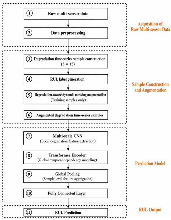
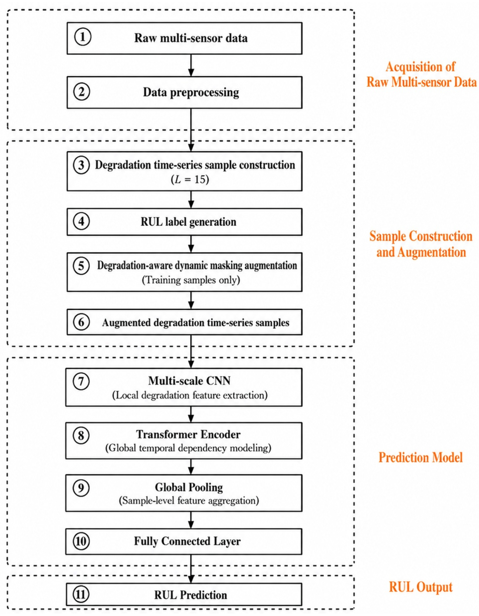
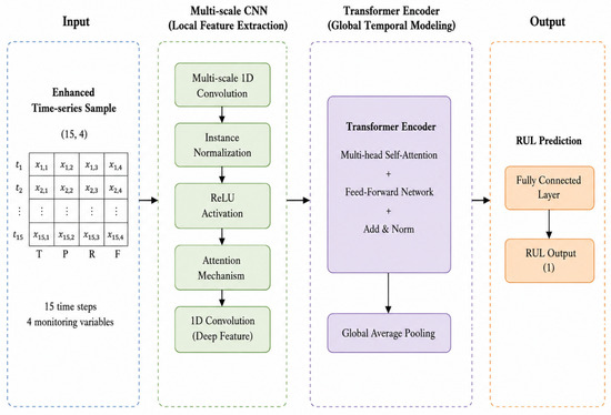
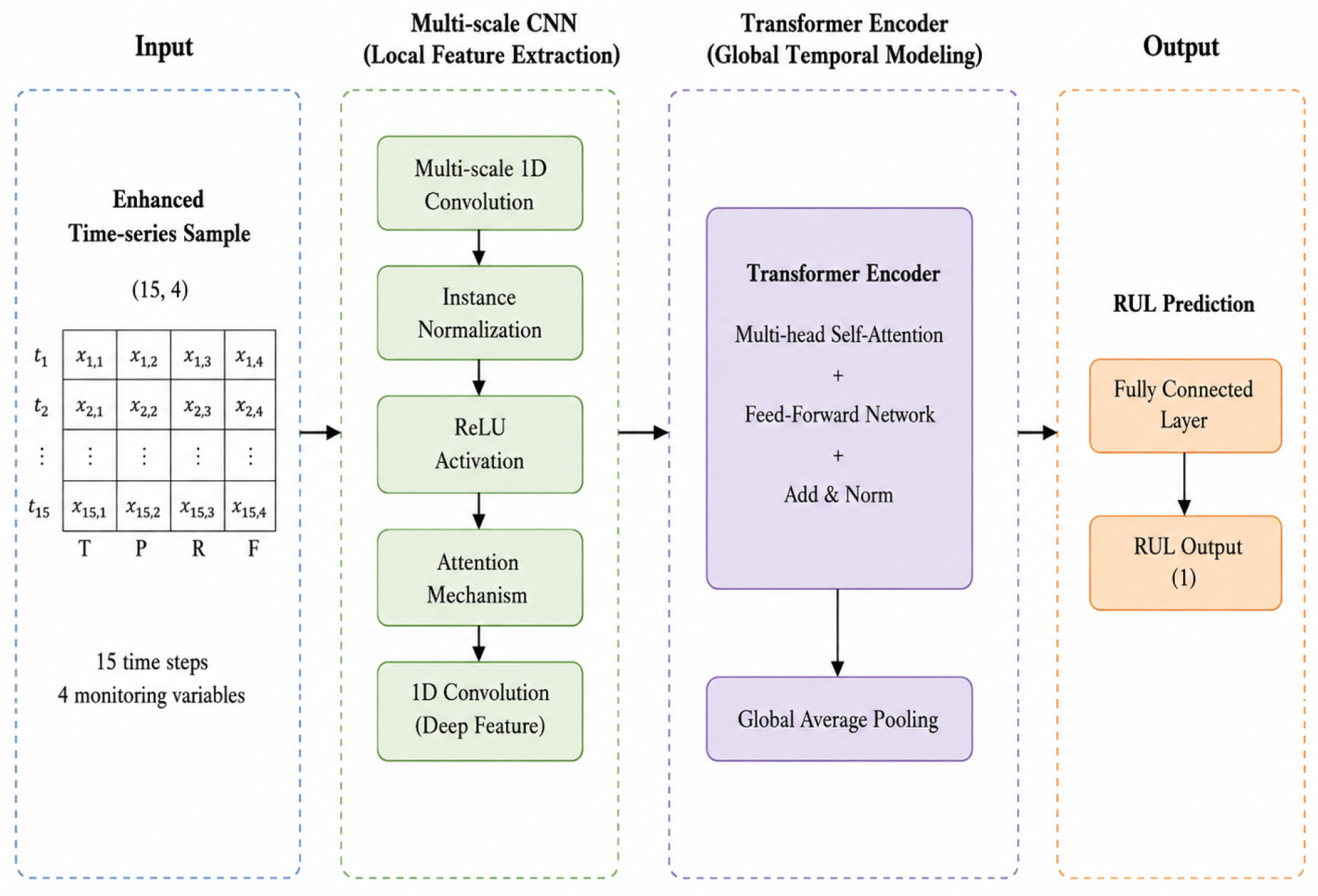
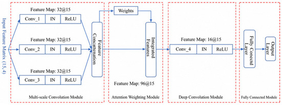
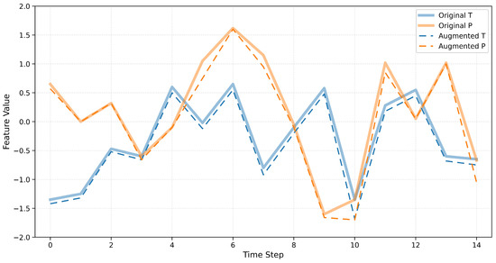
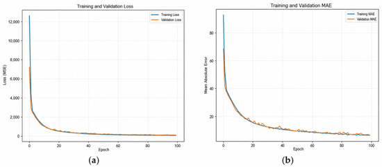
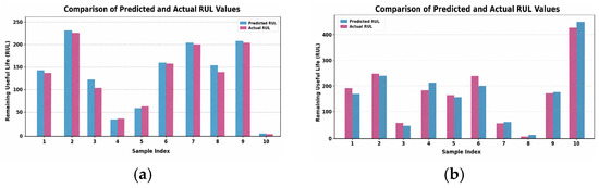
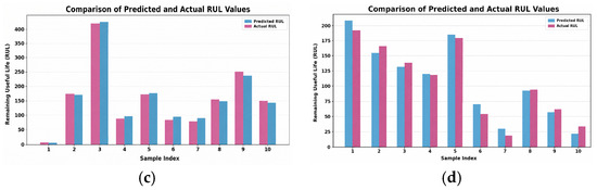
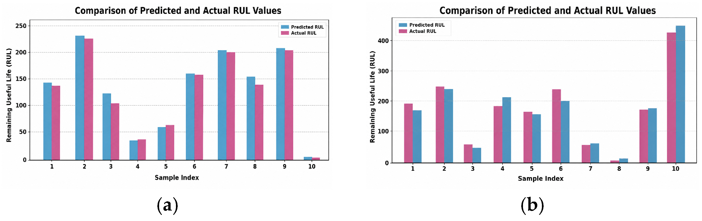
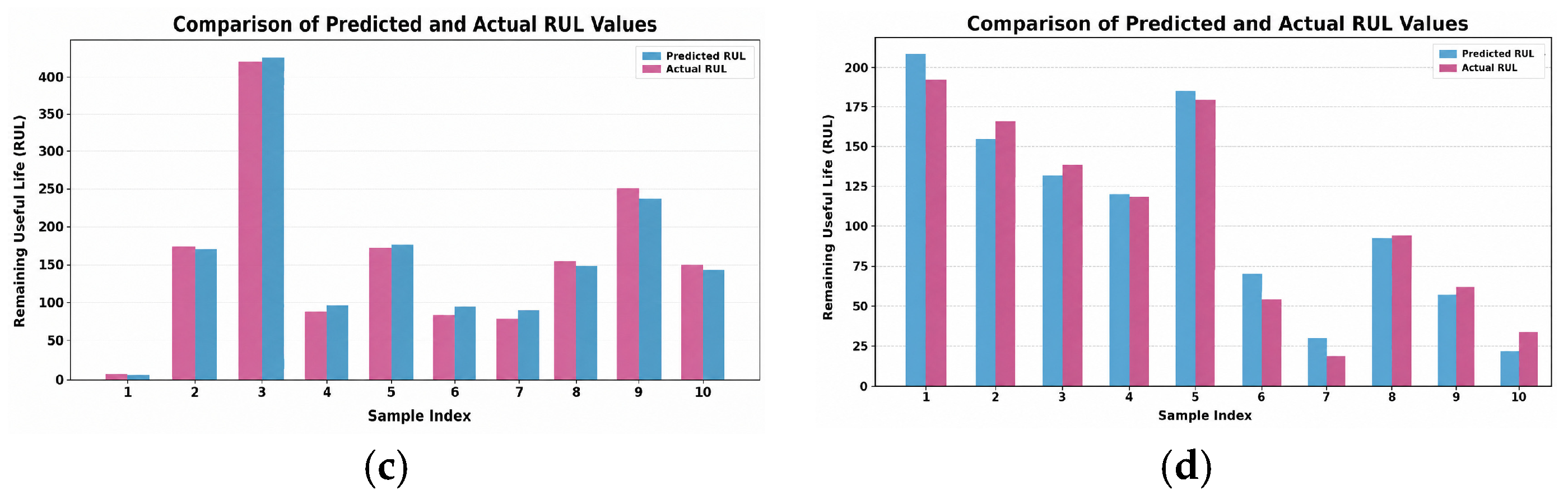
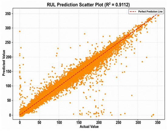
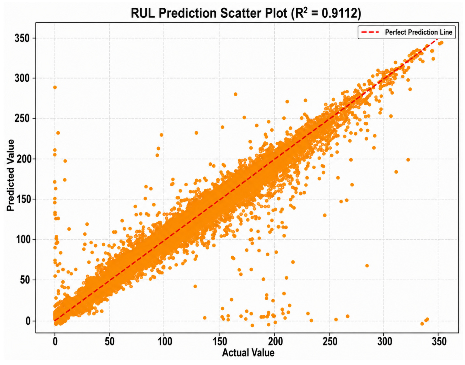
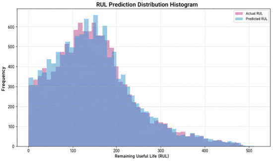
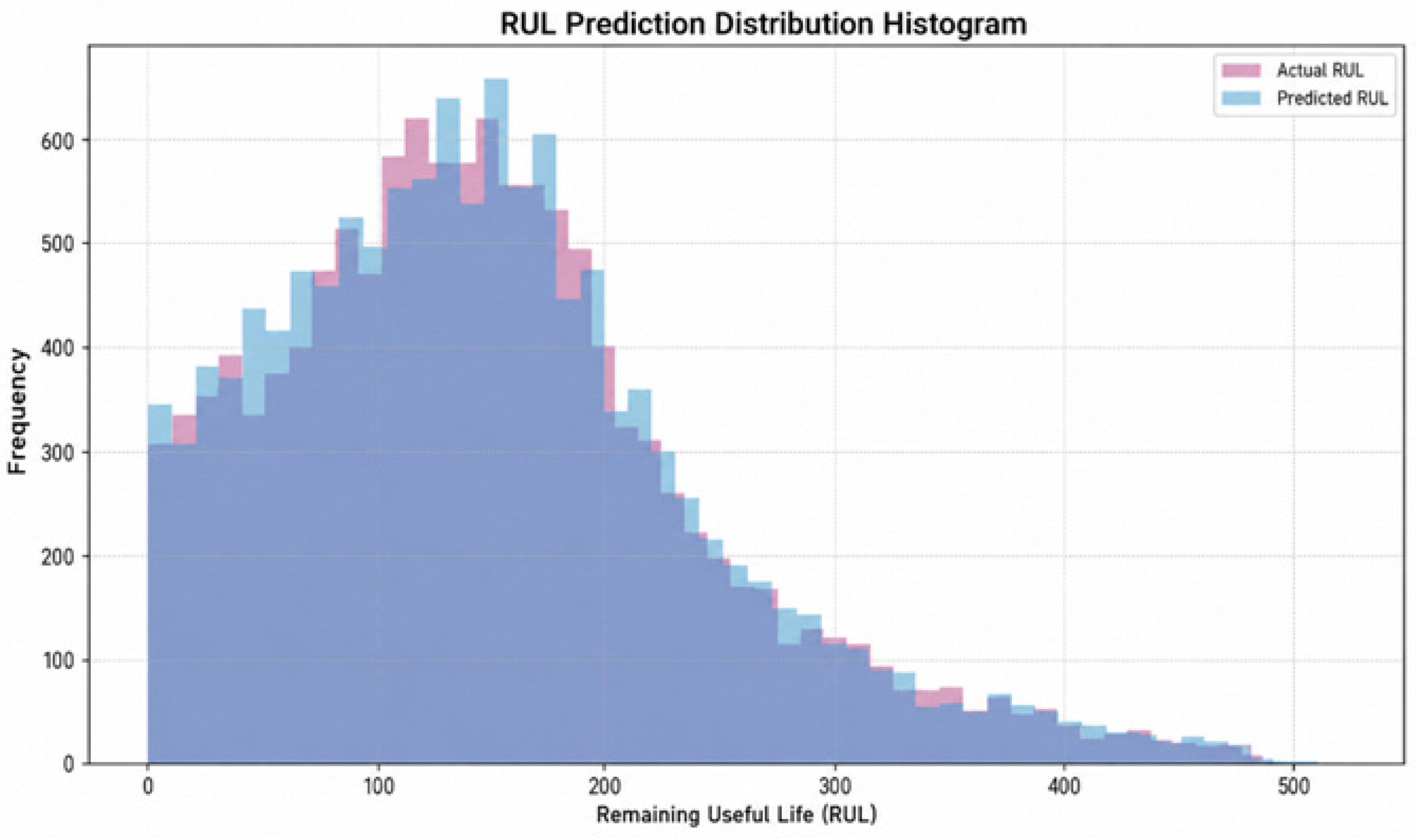

Disclaimer/Publisher’s Note: The statements, opinions and data contained in all publications are solely those of the individual author(s) and contributor(s) and not of MDPI and/or the editor(s). MDPI and/or the editor(s) disclaim responsibility for any injury to people or property resulting from any ideas, methods, instructions or products referred to in the content. |
© 2026 by the authors. Licensee MDPI, Basel, Switzerland. This article is an open access article distributed under the terms and conditions of the Creative Commons Attribution (CC BY) license.