Article

Prediction and Optimization of Freeform Impeller Machining Parameters Using a Hybrid Taguchi-Artificial Neural Network Model with the Levenberg–Marquardt Algorithm

School of Mechanical Engineering, Tianjin University, Tianjin 300354, China
*
Author to whom correspondence should be addressed.
Machines 2026, 14(8), 944; https://doi.org/10.3390/machines14080944
Submission received: 10 July 2026 / Revised: 6 August 2026 / Accepted: 12 August 2026 / Published: 17 August 2026
(This article belongs to the Special Issue Surface Engineering Techniques in Advanced Manufacturing)

Abstract

Freeform machining of impellers involves extended cycle times, leading to high energy consumption and costs necessitating efficient process optimization. This study develops a CAD/CAM-integrated hybrid Taguchi-Artificial Neural Network (ANN) model to optimize machining parameters for a freeform impeller. Four controllable factors, namely cutting feed ( C f ), feed Z ( F z ), retract feed ( R f ), and cutter diameter ( C D ), were investigated at five levels using an L25 orthogonal array, with machining time as the response. Taguchi analysis identified cutting feed as the most dominant factor, while retract feed was insignificant, and a first-order regression model yielded an R2 of 95.88%. A two-layer feedforward neural network with six hidden neurons achieved an R2 of 0.9999 and a mean absolute error of 0.0976 min. To rigorously validate generalization, leave-one-out cross-validation was employed, identifying three hidden neurons as optimal with a cross-validated R2 of 0.9823, RMSE of 0.5350 min, and MAE of 0.3429 min. The final model trained on all samples achieved an R2 of 0.9996. Comparison with a quadratic regression model on the same test set confirmed the superior predictive capability of the ANN ( R 2 = 0.9992 vs. 0.9983 ). Optimal parameters ( C f = 12,000   m m / m i n , F z = 600   m m / m i n , R f = 4000   m m / m i n , C D = 6   m m ) were validated through simulation, yielding a machining time of 11.05 min, representing a 52.6% reduction from 23.32 min. The hybrid Taguchi–ANN framework effectively optimizes freeform impeller machining, significantly enhancing productivity while maintaining process reliability.

1. Introduction

The manufacturing of complex freeform surfaces, particularly impellers, presents significant challenges in modern precision engineering due to their intricate geometries and stringent quality requirements. Impellers are critical components in various industries, including aerospace, automotive, and power generation. In these industries, their aerodynamic performance directly impacts overall system efficiency. The machining of such components demands careful selection of cutting parameters to balance productivity, surface quality, and tool life while minimizing manufacturing costs. This study aims to reduce machining time for freeform impellers by optimizing machining parameters. To achieve this, it introduces a CAD/CAM modeling framework coupled with a hybrid predictive model that integrates the Taguchi method and an artificial neural network (ANN).
Machining time ( M t ) serves as a fundamental performance metric in manufacturing economics, directly influencing production throughput and unit cost. For freeform surfaces, the relationship between cutting parameters and M t is complex and nonlinear. This complexity stems from factors like toolpath geometry [1], material removal rates [2], and machine tool dynamics [3]. Traditional one-factor-at-a-time optimization approaches fail to capture interactions between parameters and often lead to suboptimal solutions.
The Taguchi optimization technique has been widely used by researchers to optimize the machining of various metals [4,5,6,7,8] and other optimization [9]. Originally developed for enhancing industrial process design, this method serves as a robust experimental approach for identifying optimal conditions. This methodology operates by arranging experiments according to specifically designed orthogonal arrays, where each combination of control factor levels appears with equal frequency across different columns. In machining research, data is collected through repeated observations for each factor combination [10]. This allows researchers to investigate output parameters of interest, such as surface roughness or machining time. This approach guarantees that the assessment of how various technological parameters influence the desired outcomes is reliable. As a result, researchers can efficiently identify optimal cutting conditions with minimal simulation runs.
The Taguchi method, recognized for its robustness and predictive capability, has been widely applied to optimize machining parameters for various hardened steels and other materials. Notable applications include studies on Al-6061 [11], Al5059/SiC/MoS2 [6], AA7039/Al2O3 [12], aluminum-manganese alloys [13], steel 18CrNiMo7-6 [4], AISI 4340 steel [14], and AA6082/ZrSiO4 composites [15], among others. For instance, Rashid et al. [14] employed the Taguchi technique to optimize the machining of AISI 4340 steel, utilizing analytical tools such as ANOVA and regression to determine optimal parameter settings. Similarly, Tripathy and Tripathy [16] applied the Taguchi method to enhance the machining performance of H-11 steel by incorporating SiC powder into the dielectric fluid. In another study, Kumar and Parkash [17] optimized the machining of Al-B4C composites using the Taguchi approach, performing statistical analyses to evaluate the influence of various process parameters. Further investigations have extended this optimization methodology to different material systems [18,19,20].
Balaji et al. [21] investigated the influence of mixed abrasives in abrasive water jet drilling of SS304, optimizing hole quality using Taguchi-based Grey Relational Analysis and the Krill Herd Algorithm. They concluded that mixed abrasives outperformed single abrasives, with the Krill Herd Algorithm achieving prediction errors below 2% at lower computational cost than Grey Wolf Optimization. Nguyen et al. [22] addressed challenges in grinding Ti6Al4V by developing a predictive model for wheel wear using grinding force signals, adaptive neural fuzzy inference, and Gaussian process regression. Their approach enabled high-fidelity monitoring of wheel wear and surface roughness, with an average prediction error of 0.31% and 98% reliability, supporting real-time surface quality forecasting and proactive maintenance. Sikder et al. [23] proposed a multivariate process quality control framework integrating prediction-based monitoring with Taguchi systems, support vector regression, bootstrap intervals, and Nelder–Mead optimization. Industrial validation confirmed its effectiveness in predicting and preventing out-of-control scenarios, enhancing overall process performance. Despite these contributions, the validation of Taguchi-based optimization in existing studies has been predominantly confined to flat surfaces, highlighting a methodological gap in its application to more complex geometries. The present study addresses this limitation by extending the Taguchi optimization framework to freeform surface machining, specifically focusing on an impeller geometry.
Artificial Neural Networks (ANNs) offer powerful nonlinear modeling capabilities [24,25], learning directly from simulation data without requiring predefined mathematical relationships [26,27,28]. When combined with properly designed experiments, ANNs can approximate complex functions with high accuracy. This makes them suitable for machining process optimization [29,30,31,32,33]. So, the application of computational intelligence for modeling and predicting machining performance has been extensively explored. In the context of slot milling, Serin et al. [34] employed a deep perceptron neural network to establish a predictive model. This model linked fundamental process parameters such as cutting depth, feed rate, and cutting speed to key outcomes of surface roughness and energy consumption. Expanding the scope of machine learning applications, Correa et al. [35] conducted a comparative study between Bayesian networks and ANNs for predicting product quality in machining processes. Their findings demonstrated that Bayesian networks offered superior interpretability and several performance advantages over ANNs. This outcome highlights the importance of model selection in data-driven manufacturing. The integration of diverse data sources was investigated by Lin et al. [36]. They enhanced an ANN based prediction system for surface roughness in milling. This was achieved by fusing cutting parameters with real time vibration signals, thereby enriching the input space of the model with process dynamics.
Further research has focused on hybrid and alternative modeling paradigms to capture complex machining phenomena. Xu et al. [37] proposed an innovative approach using an improved case-based reasoning (CBR) methodology to predict both surface roughness and residual stress in high-speed milling. By incorporating cutting parameters and tool wear status as input features, their work demonstrated the efficacy of similarity-based reasoning in a domain often dominated by neural networks. The predictive modeling of tool degradation has also been a central theme. Quiza et al. [38] developed an ANN model employing a backpropagation training algorithm to estimate tool wear during the hard machining of D2 AISI tool steel. Their study successfully elucidated the non-linear relationship between machining conditions and tool wear, validating the ANN’s capacity to provide accurate predictions in complex operational environments. Similarly, Özel and Karpat [39] applied a backpropagation neural network to model finish hard turning of AISI H13 steel. Their model, trained on simulation data, proficiently predicted both surface roughness and tool flank wear across a range of cutting conditions. This demonstrated robust generalization capability within the investigated parameter space. Complementing these neural network-focused studies, Nalbant et al. [40] performed a critical comparative analysis between an ANN model and traditional multiple regression analysis for forecasting surface roughness in CNC turning of AISI 1030 steel. The results of their quantitative evaluation conclusively showed that the ANN model significantly outperformed the regression-based approach in terms of predictive accuracy. This underscores the superiority of non-linear models. They are better for capturing the intricate relationships in the machining process.
Advancements in machining process optimization have increasingly integrated the Taguchi method with ANN to enhance prediction accuracy and multi-response optimization. Prabhu and Vinayagam [41] applied the Taguchi L9 orthogonal array to optimize process parameters in EDM of Inconel 825, demonstrating significant improvement in surface quality. Altin Karatas and Biberci [42] conducted statistical analysis of WEDM machining parameters for Ti-6Al-4V alloy using Taguchi-based grey relational analysis coupled with artificial neural network. Zhou et al. [43] utilized Taguchi-based grey relational analysis coupled with ANN for milling of Al/SiC metal matrix composites. This demonstrated robust prediction capability under varying machining conditions. These studies confirm that the Taguchi–ANN synergy reduces experimental trials and provides a reliable predictive tool for complex, non-linear machining processes. While these contributions are significant, the validation of ANN-based models in existing studies has been largely confined to flat surfaces. This reveals a methodological gap in their application to more complex geometries. The present study addresses this limitation by extending the ANN framework to freeform surface machining, with a specific focus on impeller geometry.
Recent research has increasingly focused on integrating sustainable techniques with intelligent optimization to address the challenges of machining difficult-to-cut materials. The application of eco-friendly lubrication methods, such as Minimum Quantity Lubrication (MQL) and Nano-MQL with vegetable-based oils, has been shown to significantly improve machining performance. For instance, investigations on Inconel 718 under various environments (dry, MQL, Nano-MQL, and cryogenic CO2) have demonstrated that cryogenic CO2 and Nano-MQL can reduce cutting forces, tool wear, surface roughness, and temperature by up to 43% compared to dry machining [44]. Similarly, the use of graphene nanoplatelet (GnP)-enhanced sesame oil in MQL for milling AISI H11 steel resulted in a notable 62.5% reduction in cutting temperature and a 68.6% improvement in surface roughness [45]. These studies underscore the effectiveness of advanced lubrication strategies in enhancing both productivity and sustainability.
The use of advanced computational models is becoming indispensable for predicting and optimizing these complex processes. Artificial Neural Networks (ANNs) have proven highly effective, often achieving prediction accuracies with R2 values exceeding 0.97 for multiple machining responses [44,45,46]. While the Taguchi method is widely used for designing experiments and identifying significant parameters [46,47,48], its first-order linear regression models can be limited when capturing highly non-linear behaviors. To overcome this, hybrid methods have gained prominence. For example, an ANN-Genetic Algorithm (GA) hybrid was found to provide superior global search capabilities, while an ANN-Particle Swarm Optimization (PSO) framework offered faster convergence for optimizing machining parameters in Inconel 718 [44]. Furthermore, research on sustainable turning of SS304 has successfully used hybrid Taguchi-Grey Relational Analysis (GRA)-ANN frameworks to optimize cutting parameters for multi-objective outcomes, identifying fluid flow rate as a critical factor [48]. Studies on optimizing tribological characteristics in Mg-Al-Si alloys have also demonstrated that ANN models outperform traditional Taguchi-based regression, achieving higher prediction accuracy [46]. In the domain of friction stir processing, Taguchi-based optimization has been effectively applied to enhance joint strength in AA8011 reinforced with SiC nanoparticles, where tool rotational speed, feed rate, and tool tilt angle were identified as critical parameters influencing yield strength, ultimate tensile strength, and hardness [47]. These recent findings collectively highlight the trend towards creating intelligent, hybrid frameworks that synergize the strengths of statistical design of experiments (like Taguchi), multi-criteria decision-making (like GRA), and powerful AI-based predictive models for robust and efficient process optimization.
While Taguchi-based optimization has been applied to freeform geometries in previous studies, the novelty of this work lies not in the application of the Taguchi method to freeform surfaces per se, but rather in the integration of three key elements: (1) a comprehensive CAD/CAM framework specifically tailored for impeller machining with custom stock geometry optimization; (2) the hybrid Taguchi–ANN approach where the Taguchi design provides structured experimental data and the ANN captures complex nonlinear interactions that linear models inherently miss; and (3) the systematic validation through leave-one-out cross-validation and comparison with quadratic regression on the same test set, which provides rigorous evidence of the ANN’s superior predictive capability. This integrated framework for freeform impeller optimization, combining experimental design, nonlinear modeling, and cross-validated performance assessment, has not been previously reported in the literature.
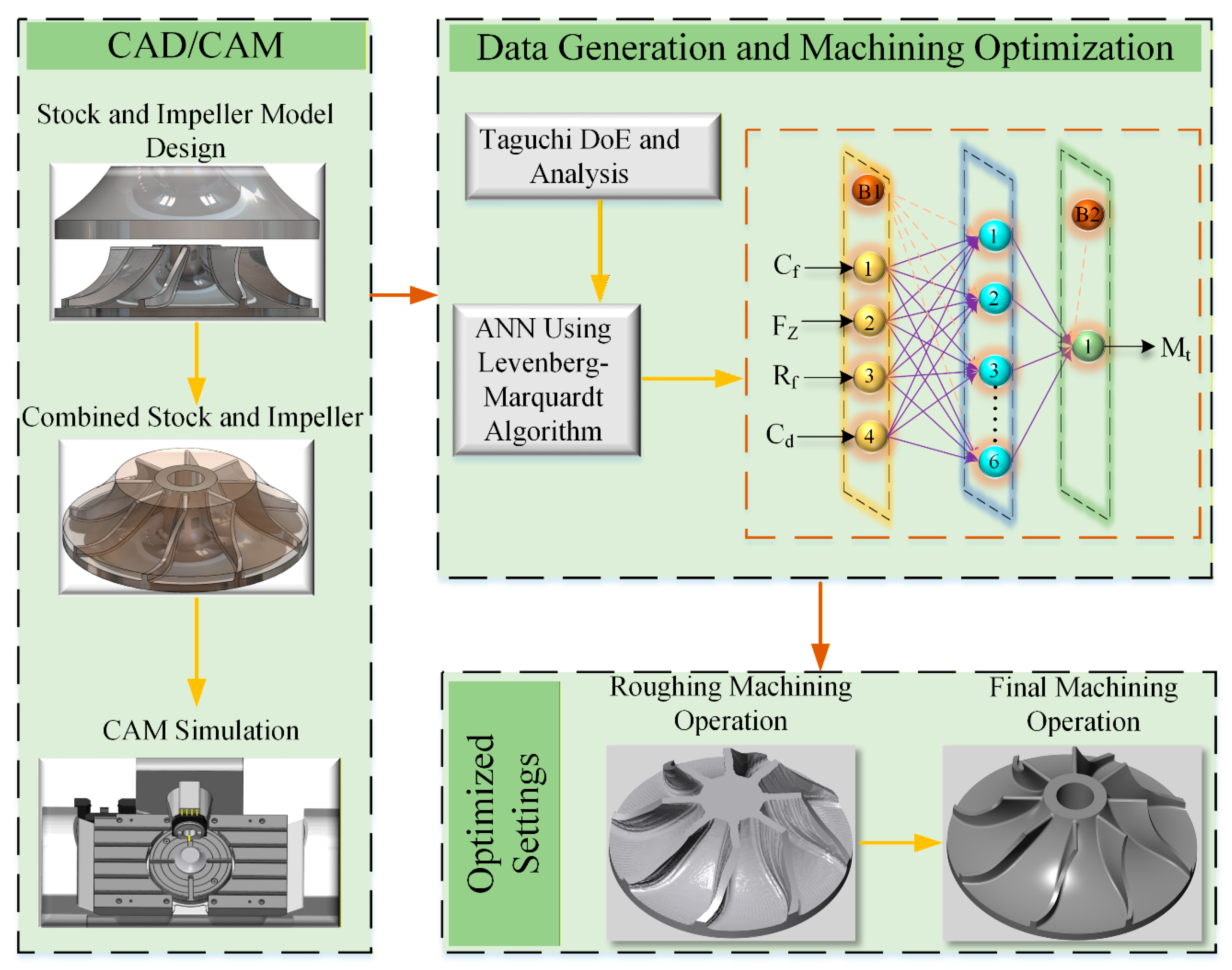
This study addresses the critical need for efficient impeller machining by developing hybrid Taguchi–ANN optimization methods to solve the aforementioned problems. As shown in Figure 1, the research began with the execution of the CAD/CAM process for impeller manufacturing, followed by the implementation of a Taguchi Design of Experiments (DoE) to structure the simulation data based on selected cutting parameters. Machining times were recorded, and both Taguchi-based analysis and ANN modeling were performed using the generated dataset. Taguchi DoE provides structured, information-rich simulation data while identifying main effects and interactions. Meanwhile, ANN captures complex nonlinear relationships to deliver accurate predictions. To achieve this, this study introduces several innovations:
  • CAD/CAM Strategies: This research presents a strategic framework for employing CAD/CAM software in modeling, simulation, data generation, and G-code preparation to support experimental machining.
  • Hybrid Taguchi–ANN Optimization Framework: Integration of Taguchi robust experimental design with ANN nonlinear modeling capabilities for comprehensive process optimization of freeform impeller machining.
  • Parameter Investigation: Comprehensive analysis of four critical cutting parameters ( C f , F z , R f , and C d ) at five levels each. This provides detailed insights into their individual and combined effects on machining time.
  • Statistical Validation of Factor Significance: Through ANOVA and S/N ratio analysis, C f was quantified as the overwhelmingly dominant factor with a 95.46% contribution, while R f was identified as statistically insignificant ( p > 0.05 ). This enables focused parameter selection.
  • High-Accuracy ANN Architecture: A two-layer feedforward network with six hidden neurons was developed, achieving exceptional predictive accuracy ( R = 0.9999 , M A E = 0.0976 min). The results demonstrate the effectiveness of Levenberg–Marquardt training with early stopping regularization.
  • Quantifiable Performance Improvement: Simulation-based validation achieved a 52.6% reduction in machining time (from 23.32 to 11.05 min), with a corresponding increase in material removal rate from 1501   m m 3 / m i n to 3167   m m 3 / m i n .
  • Comparative Model Assessment: Systematic comparison between Taguchi regression and ANN predictions reveals superior ANN accuracy ( M A E = 0.0976 min versus Taguchi M A E = 0.8563 min) and establishes the value of hybrid approaches.
  • Practical Implementation Framework: As part of this research, normalized preprocessing protocols, Nguyen–Widrow weight initialization strategies, and denormalization equations were developed. Together, these components form a framework that enables direct industrial application of the optimized parameters.
Despite the contributions of this research, we acknowledge its limitations. The analysis combining Taguchi methods with an ANN was performed on simulation data for the impeller, as a full set of physical experiments was not feasible. Executing 25 distinct trials would have required an individual workpiece each time, resulting in unsustainable consumption of both materials and energy. Nevertheless, the core innovations of this study address critical issues in freeform machining and represent a meaningful contribution to the field of precision manufacturing. This study focuses primarily on machining time minimization, even though surface quality and machining accuracy are crucial considerations in any machining operation. Machining time was selected as the primary output because it is the most direct and significant contributor to manufacturing productivity and cost reduction in freeform impeller manufacturing. The machining strategy was configured to maintain process reliability and achieve acceptable surface quality. This included tool selection (a 4-flute bull-nose end mill) and depth of cut parameters (0.5 mm radial and axial), as confirmed by the successful completion of the finishing operation. Future work will extend this framework to multi-objective optimization incorporating surface quality, tool wear, and energy consumption.
The remainder of this paper is organized as follows: Section 2 presents the methodology of the research. Section 3 presents the results and discussion of the machining optimization. Section 4 presents the confirmation of experiments and method comparisons. Finally, Section 5 concludes the paper.

2. Research Methods

2.1. Freeform Shape Design

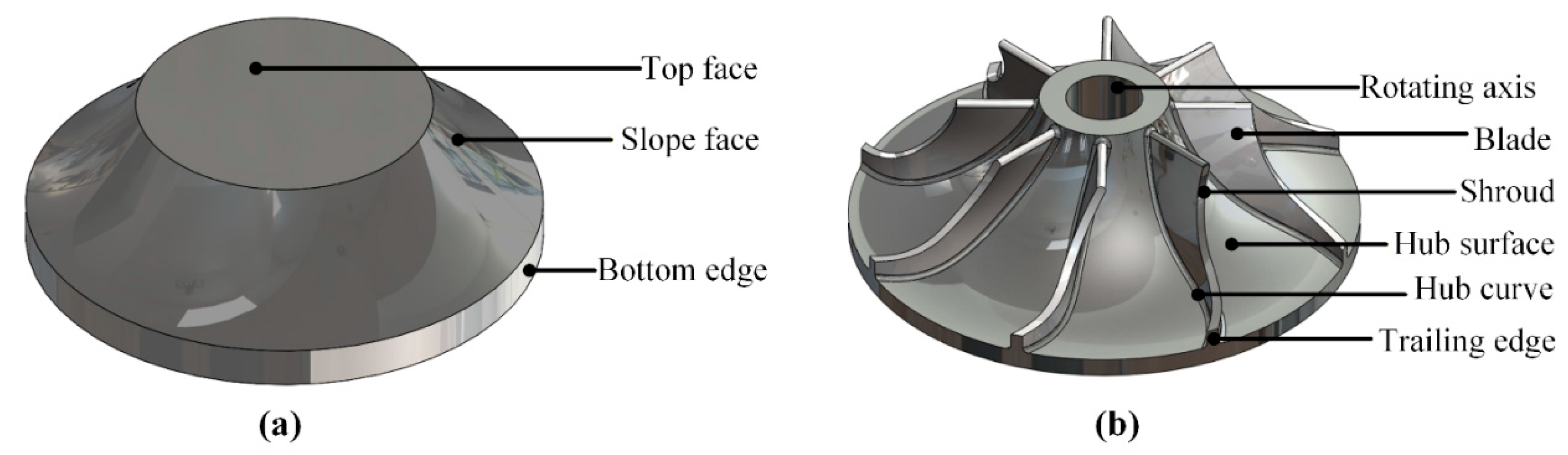
As depicted in Figure 2, the target freeform impeller and its corresponding stock were designed in SolidWorks 2021. The stock represents the raw material from which the final component is machined. In this study, the stock geometry was specifically optimized to reduce machining time, minimize feed rate fluctuations, prevent tool-workpiece collisions, and mitigate excessive tool wear.
A critical step in the workflow involved aligning the coordinate systems between the designs and manufacturing environments. The CAD model was intentionally constructed in SolidWorks with the understanding that its Y-axis corresponds to the Z-axis in SolidCAM 2021. This alignment mirrors the standard configuration of a physical vertical machining center (VMC). Consequently, the toolpaths and G-code generated in the virtual environment can be directly transferred to the CNC machine for production.
During the CAD modelling, 1060 alloy was selected as the material for both the stock and the impeller. The stock was designed as a custom freeform volume with key dimensions of 61.02 mm (upper diameter), 106.12 mm (bottom diameter), 33.10 mm (height), and an 80.00 mm radius for its contoured face. The target impeller has a total height of 33.00 mm and a bottom diameter of 106.00 mm, with a central hub radius of 40.00 mm. The blade thickness (shroud) is 1.00 mm; the blade extends from a height of 14.92 mm at its upper part to 4.00 mm at its bottom part, maintaining a 4.00 mm clearance from the base of the impeller. The central hole of the impeller has an inner diameter of 16.00 mm and an outer diameter of 27.00 mm.

2.1.1. Assembly for CAM Setup

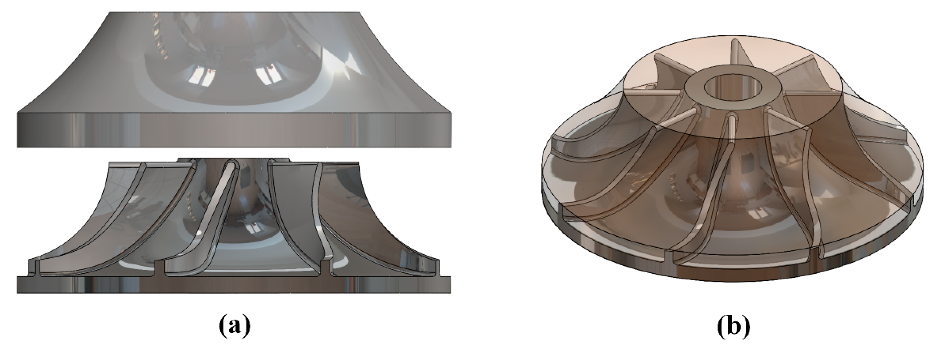
After the impeller and its stock were designed as separate components, they were assembled to transition from design to manufacturing process planning. This assembly of the target geometry with its raw stock is necessary for CAM simulation. As illustrated in Figure 3, the definitive CAD models of the impeller and the stock are spatially combined within the simulation environment. Figure 3a provides an exploded view, clearly delineating the two primary components. Figure 3b shows the combined configuration where the stock volume envelops the impeller. This assembly defines the crucial initial material state for machining. This state forms the foundational reference for the CAM software (SolidCAM 2021), from which all subsequent toolpath generation and material removal simulation are computed.

2.1.2. Machining Simulation Setup

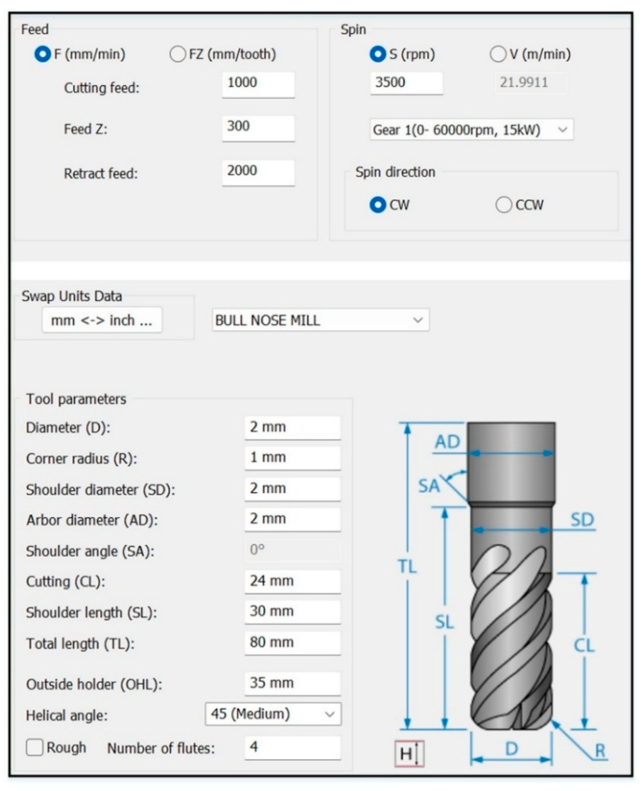
The machining for the freeform impeller was configured and conducted in SolidCAM 2021. As shown in Figure 4, the initial setup for the roughing operation was defined by selecting a cylindrical bull-nose end mill as the primary cutting tool. Key machining parameters including Cutting feed ( C f ), Feed Z ( F Z ), Retract feed ( R f ), and Cutter diameter ( C D ) were set for the simulation. The specific values were a C f of 6000 mm/min, an F Z of 200 mm/min, an R f of 2000 mm/min, and a C D of 6 mm. The toolpath was generated using a 3D peripheral milling strategy, which was calculated to follow the contours of the impeller efficiently. Under this initial configuration, the CAM software calculated a total machining cycle time of 23.3167 min, which served as the benchmark for subsequent optimization analysis.
This calculated time represents the estimated duration for a single workpiece under the defined static parameters. The simulation confirmed the feasibility of the toolpaths, showing no collisions and a consistent material removal rate. The choice of a bull-nose end mill was important for balancing surface finish quality against machining time in this first simulation pass. These initial parameters and the resulting cycle time provided the essential reference data. This data was required to evaluate the effectiveness of the later predictive model and optimization framework.

2.1.3. Cycle Time Determination and Machine Dynamics Modeling

The machining time ( M t ) reported in this study represents the total cycle time recorded from SolidCAM 2021 upon completion of the simulation for the defined 3D peripheral milling toolpath. This recorded time accounts for both cutting and non-cutting movements. The simulation integrates the kinematic model of the Hermle C20U 5-axis CNC machine (manufactured by Hermle AG, Gosheim, Germany), which includes:
1.
Programmed Feed Rates: The specified cutting feed ( C f ), feed Z ( F z ), and retract feed ( R f ) are applied to the respective G01 linear and G00 rapid positioning commands.
2.
Acceleration and Deceleration: The post-processor and machine simulation include acceleration and deceleration phases based on the machine’s default dynamic parameters, ensuring that rapid and feed movements do not exceed the machine’s axis acceleration limits. This prevents unrealistic instantaneous speed changes.
3.
Axis Synchronization: The time for the C and A rotary axes to synchronize with the linear axes (X, Y, Z) is included. The simulation calculates the path interpolation time based on the shortest synchronized motion that adheres to the machine’s kinematic constraints.
4.
Rapid Traverse (G00): All non-cutting repositioning moves are calculated at the machine’s maximum rapid traverse rate (default for the Hermle C20U), which forms the baseline for the R f .
5.
Spindle Limits: The simulation does not include a dynamic calculation of spindle power or torque limits, as these are not typically limiting factors for the finishing toolpaths employed in this study. The toolpath and feed rates are designed to ensure that the cutting forces stay within the recommended limits for the 4-flute bull-nose end mill and 1060 alloy material.
It is important to note that this study’s cycle time is based on a high-fidelity virtual simulation using industrial-grade CAM software. While it accounts for the kinematic and dynamic models of the machine, it does not incorporate real-world stochastic effects like tool wear progression, thermal expansion of the machine structure, or variations in material hardness. These factors could slightly increase machining time in a physical production environment. However, the simulated cycle time serves as a highly accurate and reliable baseline for comparing the relative impact of different cutting parameters in the optimization process.

2.2. Experimental Design and Parameters

In this paper, four controllable factors were selected based on preliminary trials and machining experience. These factors are Cutting feed ( C f ), Feed Z ( F Z ), Retract feed ( R f ), and Cutter diameter ( C D ). Each factor was tested at five levels, as detailed in Table 1. To effectively capture the effects of each parameter, an L25 (54) orthogonal array was adopted, requiring 25 simulation runs. This array accommodates the level factors and maintained a manageable number of experiments.
The design can be represented as a matrix X (size n   ×   k ), where each row corresponds to an simulation run with coded or actual factor levels. Also, each column represents a factor or an intercept term.
The selection of the four controllable factors was based on preliminary machining studies and established practices in freeform machining optimization. The factor selection process follows the methodology established in [10], where cutting feed, feed rate, and cutter diameter were identified as the most influential parameters affecting machining time. In that study, cutter diameter contributed 95.52% to machining time variation, cutting feed contributed 4.42%, and feed Z contributed 0.06%. This established a clear hierarchy of factor influence. Building upon these findings, we extended the optimization framework to impeller geometry while incorporating an additional factor (retract feed) to capture the influence of non-cutting movements on total machining time. The five levels for each factor were selected to span the operational ranges recommended by the tool manufacturer and SolidCAM machining database. This ensured practical applicability while covering a sufficiently broad parameter space. This systematic selection process ensures comprehensive coverage of the machining parameter space along with experimental efficiency through the L25 orthogonal array.

2.2.1. Performance Characteristic

In this study, the primary performance characteristic was the total M t , measured in minutes. The Signal-to-Noise (S/N) ratio with a “smaller-is-better” characteristic was calculated for each run to evaluate parameter robustness against noise, and also to minimize process variability. The S/N ratio (η) for the i-th observation was computed as:
η i = 10 l o g 10 1 n j = 1 n y i j 2
where y j i is the measured machining time for the i t h run in the j t h trial and n is the number of repetitions. Subsequent analysis involved Analysis of Variance (ANOVA) to quantify the statistical significance and contribution of each factor, followed by Main Effects Plots to visualize trends. Also, regression analysis was performed to establish a predictive linear model for M t based on the input parameters.

2.2.2. Regression Model Formulation

In this research, first-order multiple linear regression model was postulated to relate the machining time ( M t ) to the four input parameters. The general form of the model is:
M t = β 0 + β 1 C f + β 2 F z + β 3 R f + β 4 C D + ε
where M t is the predicted machining time, β 0 is the intercept constant, β 1 ,   β 2 , β 3 , β 4 are the regression coefficients for C f , F z , R f , and   C D . Also, ε is the random error term (assumed to be normally distributed with mean zero). In matrix notation, the model for all n observations is expressed as:
y = X β + ε
where
y = M t 1 M t 2 M t n ,   X = 1 1 1 C f 1 C f 2 C f n F z 1 F z 2 F z n R f 1 R f 2 R f n C D 1 C D 2 C D n ,   β = β 0 β 1 β 2 β 3 β 4 ,   ε =   ε 1   ε 2   ε n
The vector of the regression coefficient β ^ was estimated using the least squares method, as shown in Equation (5).
β ^ = ( X T X ) 1 X T y
The Taguchi analyses were conducted using Minitab 21 statistical software. The fitted regression equation was subsequently used for prediction and optimization. The significance of each model coefficient was tested using the t-statistic. Also, the overall model adequacy was assessed via ANOVA, R-squared ( R 2 ), adjusted R 2 and predicted R 2 statistics.

2.3. ANN Structure and Configuration

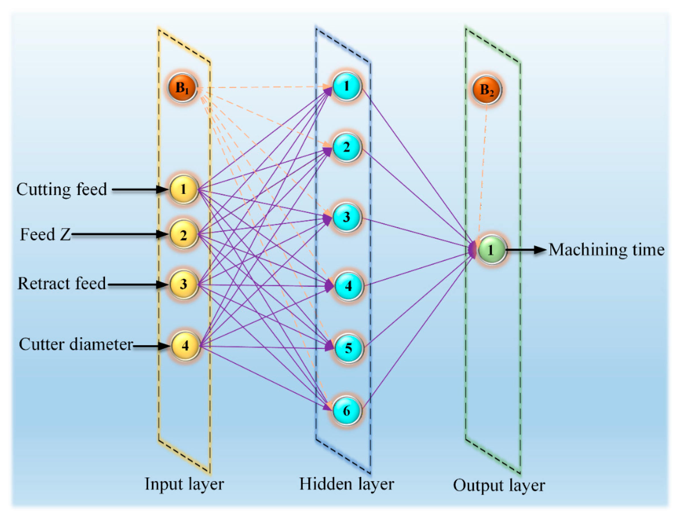
After conducting the Taguchi method, an ANN was then performed using the arranged data using Taguchi DOE. As shown in Figure 5, a two-layer feedforward neural network was designed for this study. The network consists of an input layer with four neurons corresponding to the input parameters and a single hidden layer containing six neurons. The output layer consists of one neuron representing the predicted machining time. The hidden layer employs the hyperbolic tangent sigmoid transfer function, while the output layer uses a linear transfer function. This configuration was selected following the universal approximation theorem. This theorem suggests that a single hidden layer with sufficient neurons can approximate any continuous function given appropriate training. The ANN codes, data-split indices, and random seed details are all provided in the Supplementary Material.

2.3.1. The Dataset

The dataset comprises 25 observations collected from machining operations. Four input parameters were used to predict the output variable. The input parameters are cutting feed, Feed Z, retract feed, and cutter diameter. The output variable is machining time, measured as the time required to complete the machining operation. Each observation in the dataset represents a unique combination of these input parameters and the resulting machining time.

2.3.2. Preparing the Data for Network Training

Before training, both input and output data were normalized to improve network performance and training stability. The normalization process maps the raw data to the range [ 1 ,   1 ] using the following transformation:
x n o r m = 1 + g a i n × x o f f s e t
For each input variable, the gain and offset values were computed from the training data as:
g a i n = 2 x m a x x m i n
x o f f s e t = x m i n
The same normalization parameters were subsequently applied to validation and test data to ensure consistent data transformation. After network computation, the output was de-normalized back to the original scale using Equation (9).
y ^ = y o f f s e t + y n o r m + 1 g a i n y
This preprocessing step is essential because it prevents variables with larger magnitudes from dominating the learning process and helps the activation function operate in its effective range.

2.3.3. Dividing Data into Training, Validation and Test Sets

The complete dataset of 25 observations was randomly partitioned into three subsets. Following common practice in neural network modeling, 80% of the data (19 observations) was allocated for training the network. Of the remaining 20%, half (10%, or 3 observations) was used for validation during training, and the other half (10%, or 3 observations) was reserved for final testing after training completion. The training set was used to update network weights. The validation set provided an independent assessment of network performance during training to prevent overfitting. The test set served as a final unbiased evaluation of the predictive capability of the trained model.

2.3.4. ANN Training Method

In this study, the network training was performed using the Levenberg–Marquardt backpropagation algorithm. For each hidden neuron j , the weighted sum was computed as:
z j = i = 1 4 W 1 j i · x n o r m ,   i + b 1 j
The hyperbolic tangent activation function was then applied, and it is expressed as:
a j = tanh z j = 2 1 + e 2 z j 1
At the output layer, the normalized prediction was obtained from Equation (12).
y n o r m = j = 1 6 W 2 j · a + b 2
The network performance was evaluated using the mean squared error (MSE) function as shown in Equation (13). Also, the Levenberg–Marquardt algorithm updates network weights using Equation (14).
M S E = 1 N k = 1 N ( t k y ^ k ) 2
Δ w = [ J T J + μ I ] 1 J T e
where J is the Jacobian matrix containing first derivatives of network errors with respect to weights, and it is computed as:
J = e 1 w 1 e 2 w 1 e N w 1 e N w 2           e N w 2           e N w 2           e 1 w m e 2 w m e N w m
The damping factor μ was adaptively adjusted throughout training. Training began with weights and biases initialized using the Nguyen–Widrow method. Training continued until a specific condition was met. The process would stop if the maximum number of epochs was reached, the gradient fell below a minimum threshold, or the validation error increased for six consecutive epochs. This early stopping mechanism was implemented to prevent overfitting.
The hyperbolic tangent (tanh) activation function was selected for the hidden layer for two primary reasons. First, tanh provides a zero-centered output range of [−1, 1], which facilitates faster convergence during training compared to sigmoid or ReLU, particularly for small datasets where gradient flow is critical. Second, tanh’s smooth, bounded nature and non-zero gradients across its range help prevent ‘dead neurons’ (a common issue with ReLU when many activations fall into the zero region during training). Given the limited dataset (25 samples), avoiding dead neurons is essential to ensure stable training and effective use of all available data. Studies have shown that tanh consistently achieves superior accuracy levels for small datasets compared to other activation functions. The Levenberg–Marquardt training algorithm, which we employed, is well-suited for small datasets and works effectively with tanh activation.

2.3.5. Evaluating Model Performance on Test Data

Once training was complete, the final performance of the network was evaluated using the test dataset, which had not been used at any point during the training or validation process. The three test samples were propagated through the trained network using the forward propagation equations described in Section 2.3.4 to generate predictions. As shown in Equation (16), the de-normalization step was applied to convert network outputs back to the original machining time scale.
y ^ = 11.0833 + y n o r m + 1 0.1635

2.3.6. Criteria for Assessing Prediction Accuracy

As expressed in Equation (17), the model performance was quantified using the mean squared error (MSE) as the primary metric. Additional metrics were computed to provide a comprehensive assessment, as shown in Equations (18)–(20).
M S E = 1 n i = 1 n ( t i y ^ i ) 2
R M S E = M S E = 1 n i = 1 n ( t i y ^ i ) 2
R 2 = 1 i = 1 n ( t i y ^ i ) 2 i = 1 n ( t i t ) 2
M A E = 1 n i = 1 n t i y ^ i
From the equations (Equations (17)–(20)), t i represents the actual machining time, y ^ i is the predicted value, and t is the mean of actual values. Separate performance metrics were computed for the training, validation, and test sets to assess performance across all data partitions. Also, the test set metrics provided the final measure of model generalization capability. These calculations were performed after denormalizing the network outputs to ensure errors reflect actual machining time units.
As expressed in Equation (17), the model performance was quantified using the MSE as the primary metric. Additional metrics were computed to provide a comprehensive assessment, as shown in Equations (18)–(20). The correlation coefficient (R) measures the strength and direction of the linear relationship between actual and predicted values, ranging from −1 to +1. The coefficient of determination ( R 2 ), defined in Equation (19), represents the proportion of variance in the dependent variable explained by the model, ranging from 0 to 1. While both metrics indicate model performance, R 2 is more interpretable for assessing predictive accuracy as it directly quantifies the variance explained. In this study, R 2 is used as the primary metric for evaluating model accuracy, while R is reported to indicate the strength of the linear relationship.

3. Results and Discussion

3.1. Taguchi Results

The primary objective of minimizing machining time corresponds to maximizing the S/N ratio (for “smaller-is-better”). Table 2 shows the Taguchi orthogonal array for L25 (54). The data used for the analysis in this research were based on machining simulation. This approach was necessary because executing 25 distinct experiments would have required a new workpiece for each trial, resulting in unsustainable consumption of both materials and energy. Nevertheless, the core innovations of this study address critical issues in freeform machining and represent a meaningful contribution to the field of precision manufacturing.
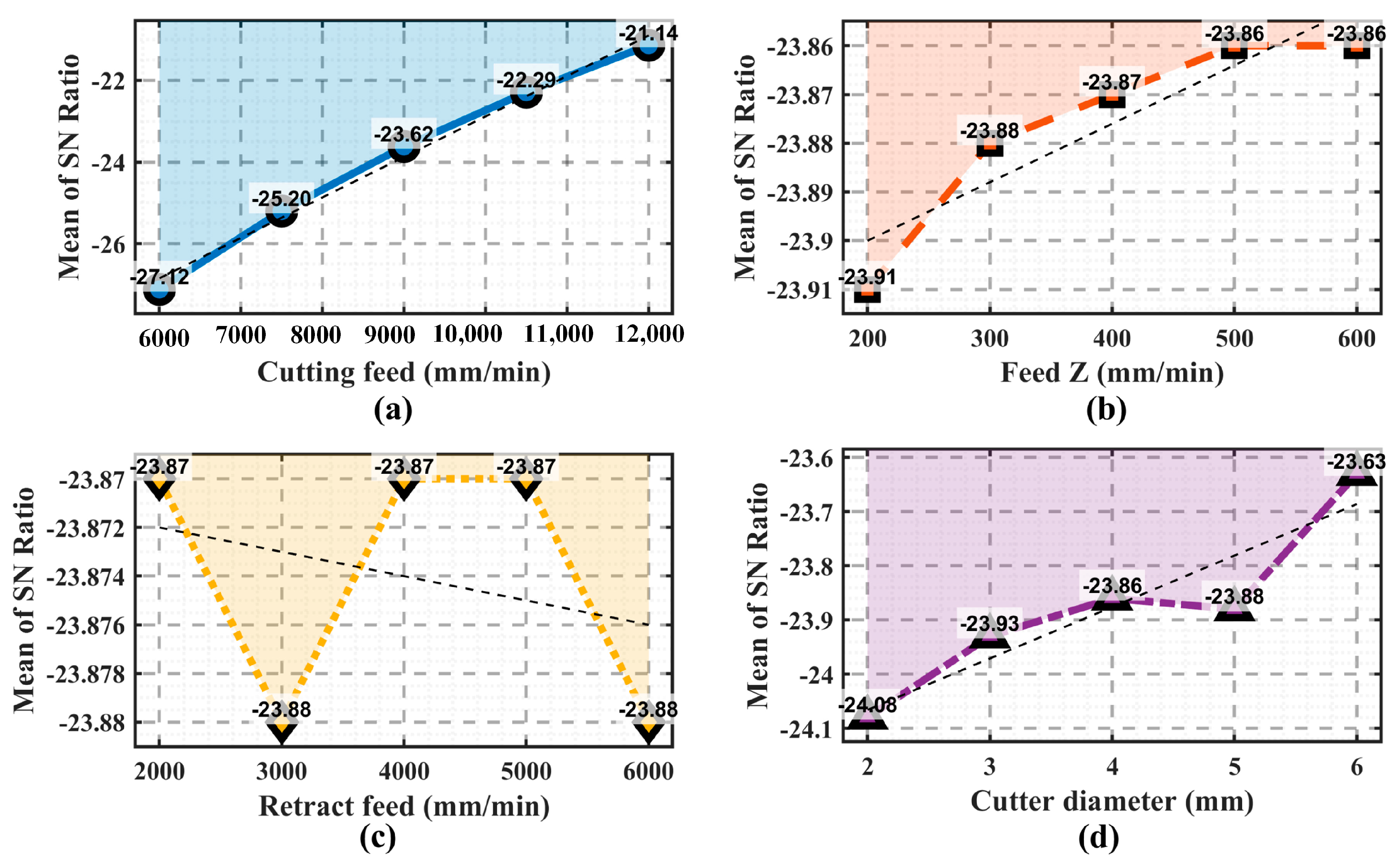
The table details the 25 simulation runs, each with its corresponding M t and S/N ratio. The response table for S/N ratios (Table 3) reveals the rank of factor influence. From the table, C f (delta = 5.98) is the most dominant, followed by C D (delta = 0.45), F z (delta = 0.05), and R f (delta = 0.02). This order is visually confirmed by the main effects plot for S/N ratios (Figure 6), where the slope for C f is markedly steeper than for other factors. The residual plots for S/N ratios (smaller is better) is shown in Figure 7. The S/N ratios in Table 2 are calculated as [49]:
S i g n a l   t o   n o i s e   r a t i o   = 10 l o g ( M t 2 )
ANOVA for S/N ratios (Table 4) provides statistical validation. The factor C f shows a high F-value (231,924.51) with a p-value of 0.000. This confirmed its overwhelming statistical significance. C D and F z are also significant with p-values of 0.000 and 0.001, respectively. R f with a p value of 0.217 is insignificant. The model demonstrates an excellent fit, with R 2 values of 100%.

3.1.1. Analysis of Mean

The response table for means (Table 5) shows a similar hierarchy of factor effects. C f again has the largest effect on the absolute M t ( d e l t a = 11.31   m i n ), with machining time decreasing progressively as C f increases from 6000 to 12,000 mm/min. C D shows a non-linear effect, with the smallest diameter (2 mm) yielding the highest mean time, due to the need for more tool passes. The main effects plot for means (Figure 8) illustrates these trends clearly.
ANOVA for the mean response (Table 6) corroborates these findings. C f accounts for the vast majority of the variation ( S u m   o f   s q u a r e = 402.882 ), with C D contributing a smaller but significant portion. Figure 9 shows the residual plots for the analysis of means.
Regarding the retention of retract feed ( R f ) in the ANN model despite its statistical insignificance ( p = 0.217 ), the ( R f ) was retained for three reasons. First, maintaining the complete L25 orthogonal array structure preserves the balanced experimental design, which is a fundamental principle of Taguchi methodology. Second, from a physical perspective, retract feed represents non-cutting movements that contribute to total machining time, and its exclusion would ignore a real process parameter. Third, the ability of the ANN to correctly identify and appropriately weight this insignificant parameter, as shown in the learned network weights (Equation (23)), validates the robustness of the model and its capacity to discern parameter significance without overfitting.
Although the retract feed ( R f ) factor has a p-value of 0.217, exceeding the conventional significance level of 0.05, it was retained as an input parameter in the ANN model for three reasons. First, maintaining the complete L25 orthogonal array structure preserves the balanced experimental design. Second, from a physical perspective, retract feed represents non-cutting movements that contribute to total machining time. Third, the ability of the ANN to correctly identify and appropriately weight this insignificant parameter (as shown in the learned network weights in Equation (23)) validates the robustness of the model and its capacity to discern parameter significance without overfitting.
The ANOVA analysis presented focuses on main effects, as the L25 orthogonal array is primarily designed for efficient main effect estimation with limited resolution for interaction effects. However, interactions between machining parameters, such as between cutting feed and cutter diameter, may influence toolpath density and material removal efficiency. While not explicitly quantified in the Taguchi ANOVA, such interactions are inherently captured by the ANN model through its non-linear mapping of input parameters to the output response. The exceptional predictive accuracy achieved by the ANN ( R 2 =   0.9999 ) suggests that any interaction effects present in the data are effectively captured by the neural network.
It is worth noting the apparent discrepancy between the S/N ratio ANOVA and the mean-response ANOVA results. In the S/N ratio analysis (Table 4), Feed Z ( F z ) and Cutter diameter ( C D ) were statistically significant ( p = 0.001 and p = 0.000 , respectively), whereas in the mean-response ANOVA (Table 6), these factors were not significant ( p = 0.772 and p = 0.184 , respectively). This difference arises because the S/N ratio analysis assesses both the mean response and variability, making it more sensitive to factors that affect process consistency, while the mean-response ANOVA considers only the average effect. In this study, Feed Z and Cutter diameter appear to influence the variability of machining time more than the mean, which explains their significance in the S/N ratio analysis but not in the mean-response analysis. Consequently, neither analysis should be presented as the sole basis for factor ranking. Instead, both analyses should be considered together to provide a comprehensive understanding of factor effects. Cutting feed ( C f ) was consistently the most dominant factor in both analyses, confirming its overwhelming influence on machining time.
It should be noted that the Taguchi S/N ratios were derived from single simulation runs without replication. While traditional Taguchi applications assess robustness against noise factors through repeated runs, the simulation-based nature of this study precluded replication. Consequently, the S/N ratios primarily reflect mean response optimization rather than process robustness. This limitation should be considered when interpreting the results for physical machining applications.

3.1.2. Predictive Model and Factor Optimization

From the coefficient analysis (Table 7), it can be seen that the coefficient for C f ( β 1 = 0.001854 ) is the only term with a substantial standardized effect ( T v a l u e = 21.52 ), which aligns with the ANOVA results. So, applying the least squares estimation method to the simulation data yielded the following fitted first-order regression equation:
M t = 33.73 0.001854 C f 0.00038 F z 0.000020 R f 0.178 C D
The normal probability plot for the regression analysis is depicted in Figure 10, and the regression model shows good accuracy, as indicated by an R 2 of 95.88%, an adjusted R 2 of 95.05%, and a predicted R 2 of 93.16%. The Taguchi analysis software calculates a predicted mean of 10.8400 min for the same configuration. Based on the objective to minimize M t , the optimal parameter settings identified from the response tables and main effects plots were C f = 12,000   m m / m i n , F z = 600   m m / m i n , R f = 4000   m m / m i n , and C D = 6   m m .

3.2. ANN Results

The neural network model was developed to predict machining time based on four input parameters (cutting feed, Feed Z, retract feed, and cutter diameter). The dataset containing 25 observations (Table 2) was partitioned into training, validation, and test sets. This resulted in 19 training samples, 3 validation samples, and 3 test samples, representing 80%, 10%, and 10% of the data respectively. This partitioning strategy ensures that the generalization capability of the model can be assessed on unseen data. It also maintains a sufficient number of training samples given the limited dataset size.

3.2.1. ANN Algorithms

The ANN was implemented as a two-layer feedforward architecture (Figure 5) with six neurons in the hidden layer and trained using the Levenberg–Marquardt backpropagation algorithm. The training procedure is summarized in Algorithms 1 and 2. Algorithm l delineates the initial phase, which commences with data preparation wherein the four input dataset is randomly partitioned into training, validation, and testing subsets.
The network parameters are initialized using the Nguyen–Widrow method to accelerate convergence. These parameters include the input weight matrix W 1 R 6 × 4 , hidden bias vector b 1 R 6 , output weight vector W 2 R 1 × 6 , and output bias b 2 R . During each training epoch, forward propagation is performed to compute the network output. The computation utilizes a hidden layer hyperbolic tangent activation function, φ ( z )   =   t a n h ( z ) , followed by a linear combination at the output layer. Subsequently, the MSE performance function is evaluated. The Levenberg–Marquardt optimization approximates the Hessian matrix as J T J , where J represents the Jacobian matrix of network errors with respect to the weights. It then updates parameters by solving ( H + μ I ) Δ w = E .
Algorithm 1. Neural network training (Levenberg–Marquardt).
1: Data Preparation
2: X = Input data matrix (4 × N) // N samples, 4 features per sample
3: T = Target output vector (1 × N) // Corresponding true values
4: // Random split to prevent ordering bias
5: Shuffle and split: 80% train, 10% validation, 10% test
6: Network Initialization
7: // MATLAB R2024a default Nguyen–Widrow initialization
8: Initialize W 1 6 × 4 ,   b 1 6 × 1 ,   W 2 1 × 6 ,   b 2 ( 1 × 1 ) with scaled random values
9: // Damping parameters control step size
10: Set μ   =   0.001 // Initial trust-region radius
11: μ i n c = 10 , μ d e c = 0.1 // Adaptive adjustment factors
12: Training Loop
13: for e p o c h   =   1 to Max Epochs: Forward propagation through the network
14: Normalized inputs: x n o r m = 1 + g a i n × ( x x o f f s e t )
15: Hidden layer: a j = t a n h ( i = 1 4 W 1 j i x n o r m ,   i + b 1 i j ) for j = 1 , , 6
16: Output layer: y n o r m = j = 1 6 W 2 j a j + b 2
17: De-normalize output: y ^ = y s t e p 1 · x o f f s e t + y n o r m + 1 y s t e p 1 · g a i n
18: Calculate error vector: e k = T k y ^ k for k = 1 , , N
19: M S E = 1 N k = 1 N e k 2
20: // Jacobian matrix J contains all first-order partial derivatives (Compute J)
21: // Approximate Hessian (second derivatives) for faster convergence
22: H J T J // Gauss-Newton approximation
23: E   =   J T e // Gradient of MSE
24: // Levenberg–Marquardt update rule
25: // Solve ( H + μ I ) Δ w = E for Δ w
26: if MSE decreases after update: Accept Δ w and shrink μ
27: μ   μ × μ d e c
28: else:
29: Reject Δ w and grow μ // Use small steps
30: μ   μ × μ i n c : (end)
31: // Early stopping to prevent overfitting
32: if validation error increases for 6 consecutive epochs: break
33: Weight Update
34: // Apply successful updates to all parameters
35: W 1 W 1 + Δ W 1 // Adjust input-to-hidden weights
36: b 1 b 1 + Δ b 1 // Adjust hidden neuron thresholds
37: W 2 W 2 + Δ W 2 // Adjust hidden-to-output weights
38: b 2 b 2 + Δ b 2 // Adjust output bias
39: end
Algorithm 2 presents the forward propagation algorithm employed during prediction. Input samples first undergo identical normalization utilizing precomputed statistics derived from the training data ( x o f f s e t and gain parameters). Following normalization, the inputs propagate through the optimized network weights and are subsequently denormalized to yield predictions in the original output domain. This method ensures consistent data transformation between training and deployment phases. It also exploits the quadratic convergence properties of the Levenberg–Marquardt algorithm in proximity to the optimum.
Algorithm 2. Feedforward neural network prediction.
1: Input
2: [ x 1 , x 2 ,   x 3 ,   x 4 ] // Raw input vector (4 features)
3: Input Normalization
4: // Map raw inputs to [ 1 ,   1 ] range using precomputed statistics
5: x 1   n o r m = 1 + 0.000333 × ( x 1 6000 )
6: x 2   n o r m = 1 + 0.005 × ( x 2 200 )
7: x 3   n o r m = 1 + 0.0005 × ( x 3 2000 )
8: x 4   n o r m = 1 + 0.5 × ( x 4 2 )
9: Hidden Layer Computation
10: // Weighted sum for each hidden neuron
11: for  j   =   1 to 6:
12: z j = W 1 j 1 · x 1 n o r m + W 1 j 2 · x 2 n o r m + W 1 j 3 · x 3 n o r m + W 1 j 4 · x 4 n o r m + b 1 j
13: // Apply hyperbolic tangent activation function
14: a j = tanh z j = 2 1 + e 2 z j 1
15: end for
16: Output Layer Computation
17: // Weighted sum of hidden layer activations using second layer weights
18: y n o r m = W 21 · a 1 +   W 22 · a 2 + W 23 · a 3 + W 24 · a 4 + W 25 · a 5 + W 26 · a 6 + b 2
19: Output Denormalization
20: // Map normalized output back to original scale
21: y ^ = 11.0833 + ( y n o r m + 1 ) 0.1635
22: Return
23: y ^ // Predicted output value

3.2.2. Trainable Parameters

The total number of trainable parameters in the network is calculated as follows. The input-to-hidden layer connections contribute 24 weights (4 inputs × 6 hidden neurons), and the hidden layer biases contribute 6 parameters. The hidden-to-output layer connections contribute 6 weights (6 hidden neurons × 1 output), and the output layer bias contributes 1 parameter, yielding a total of 37 trainable parameters.

3.2.3. Learned Weights and Biases

The trained network weights and biases provide insight into the learned representations. The input weight matrix W 1 , which connects the four input features to the six hidden neurons, is presented as:
W 1 = 1.5604 2.3287 2.3481 0.8394 1.6548 0.9167 0.0207 0.6038 0.3516 0.0066 0.8946 0.1866 0.3146 0.2956 2.8900 0.0340 0.4422 2.2494 0.1891 0.5212 2.6515 0.0760 1.6890 1.4687
Each row of this matrix corresponds to one hidden neuron, and each column corresponds to one input feature in the order. The magnitudes and signs of these weights indicate how each hidden neuron responds to different combinations of input features.
The hidden layer bias vector b 1 , which shifts the activation threshold for each hidden neuron, is:
b 1 = 1.8151 1.3783 1.7904 0.8704 1.9911 1.9954
These biases vary in magnitude, with the fourth neuron having the only negative bias of −0.8704 and the sixth neuron having a large positive bias of 1.9954. These biases position the neurons at different operating points on the tan-sigmoid activation function. Some neurons operate in the linear region near zero, while others are pushed toward saturation. This configuration allows them to act as feature detectors that respond to specific input patterns.
The output layer weight vector W 2 , which combines the hidden layer activations to produce the final prediction, is:
W 2 =   0.24874 0.0254 0.0384 1.9531 0.0514 0.08954
b 2 = 0.6800
This vector reveals that the forth hidden neuron contributes most to the output with a weight of 1.9531, followed by the first neuron with 0.24874. This suggests these neurons may have learned to recognize conditions that lead to faster machining. The output layer bias b 2 is 0.6800, providing a baseline offset for the prediction.

3.2.4. ANN Training Performance

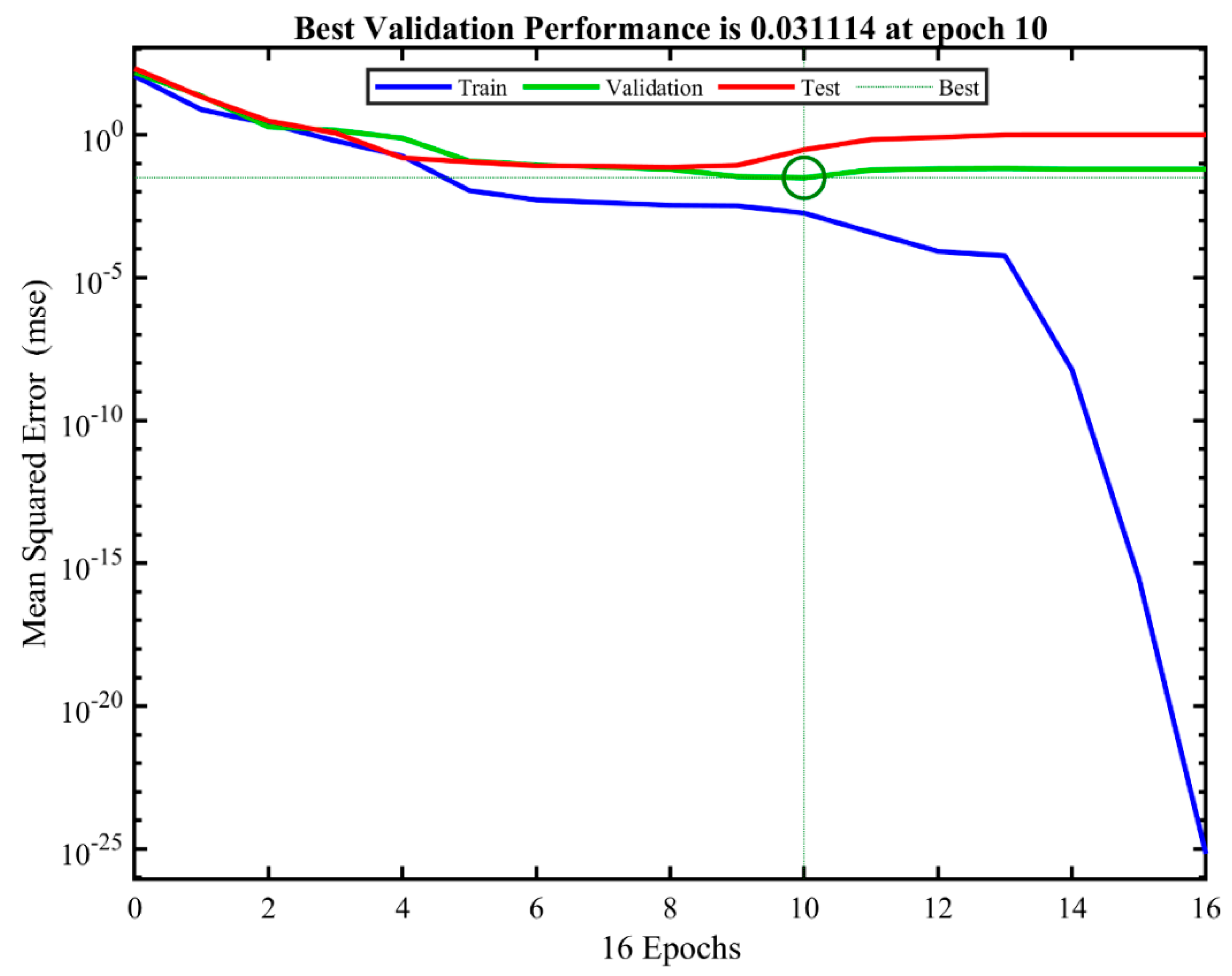
From Table 8, the training process demonstrated exceptional convergence behavior, reaching a minimum gradient condition after only 16 epochs despite a maximum allowance of 1000 epochs. This training performance plot is shown in Figure 11. This rapid convergence suggests that the Levenberg–Marquardt algorithm efficiently located a minimum of the error surface. It benefited from the well-behaved nature of the machining time prediction problem. The performance metric improved from an initial value of 114 to a final stopped value of 6.8 × 10 26 . This indicates nearly perfect fitting to the training data.
The gradient decreased from 201 to 5.02   ×   10 14 , well below the target threshold of 1 × 10 7 . This confirms successful optimization. The Mu parameter, which controls the Levenberg–Marquardt damping factor, decreased from 0.001 to 1 × 10 8 throughout training. This reflects the transition of the algorithm from gradient descent behavior toward Gauss-Newton behavior as the solution approached. The validation checks parameter reached a value of 6, exactly the stopping criterion. This indicates that the model continued to show improvement on the validation set throughout most of the training process before the minimum gradient condition was met.

3.2.5. ANN Model Evaluation

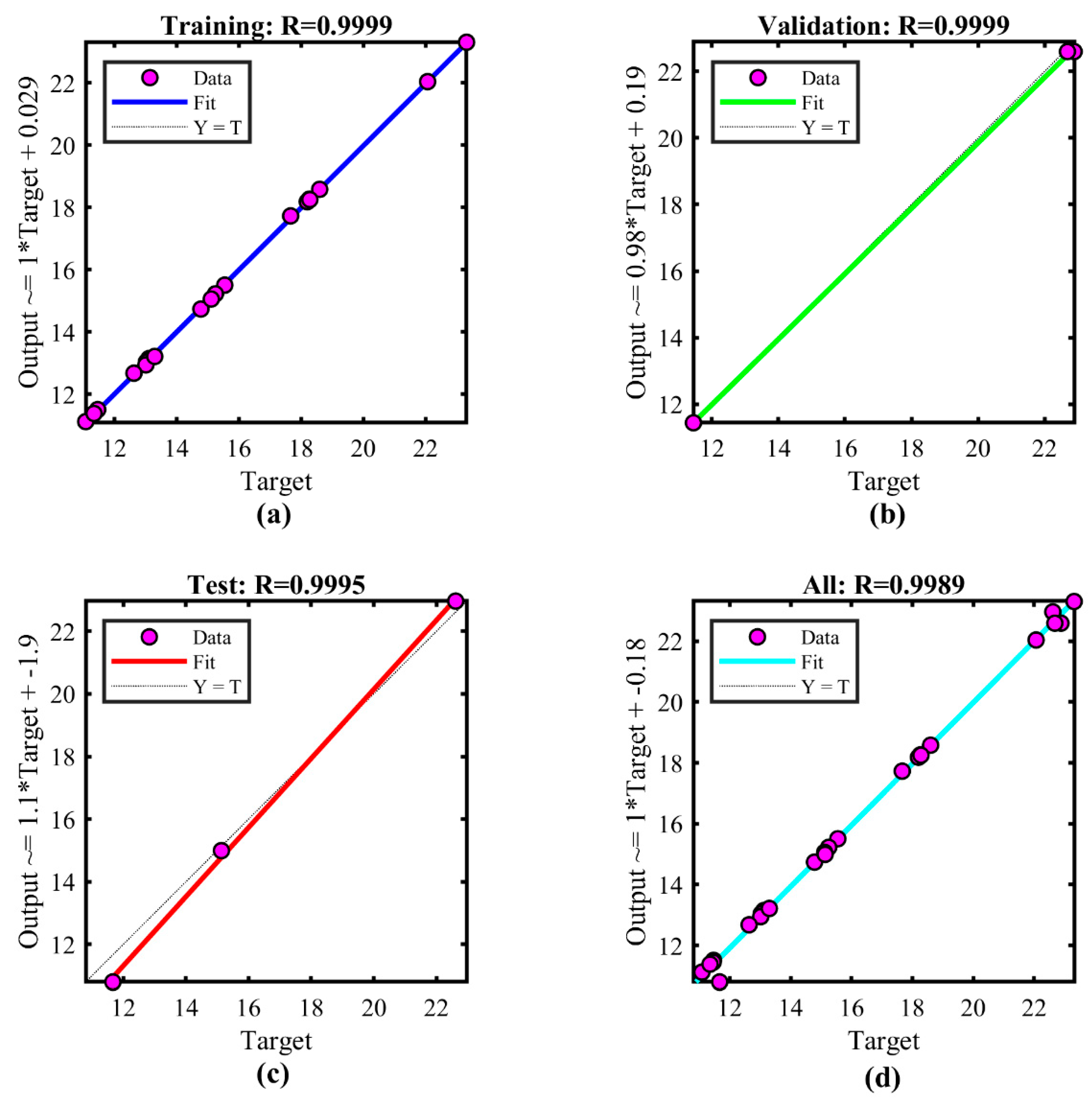
Model performance was evaluated across the three data partitions using MSE and the correlation coefficient R. As shown in Figure 12, on the training set of 19 observations, the model achieved an MSE of 0.0018 with an R value of 0.9999. This demonstrates nearly perfect correlation between predicted and actual machining times. The validation set of 3 observations produced an MSE of 0.0311 with an R of 0.9999, while the test set of 3 observations yielded an MSE of 0.2981 with an R of 0.9995.
The slight progressive increase in MSE from training to validation to test sets is expected and reflects normal generalization behavior. However, the high R values across all partitions all exceed 0.999. This indicates that the model has successfully captured the fundamental relationships between machining parameters and machining time. The small degradation in performance on the test set, despite the very limited number of test samples, suggests that the model generalizes well to unseen data points.
The root mean square error (RMSE) and mean absolute error (MAE) were computed to quantify the prediction accuracy of the model. These metrics provide information about the error distribution. RMSE is more sensitive to large errors while MAE provides a straightforward average of absolute deviations.
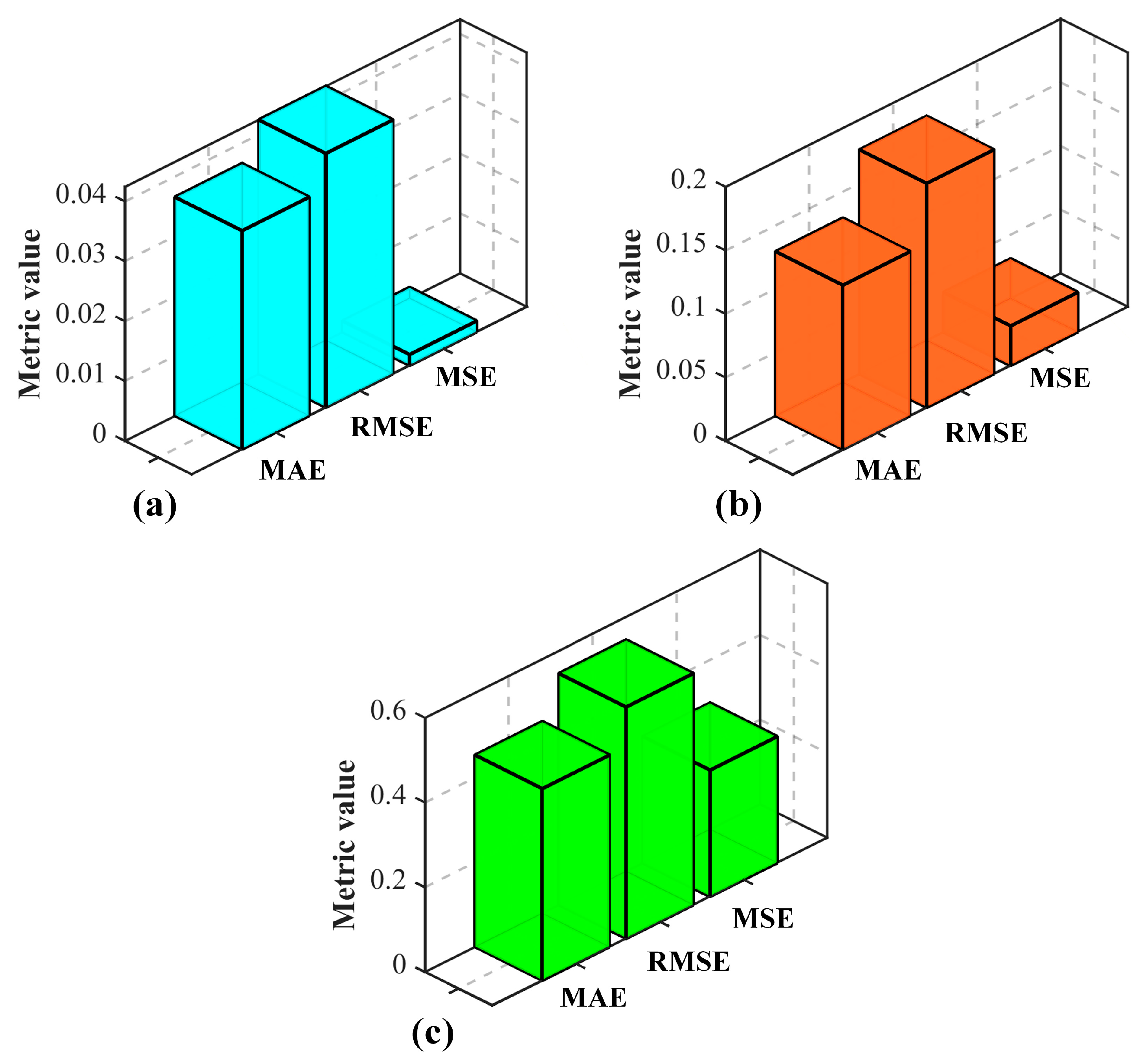
Table 9 shows the MSE and the calculated RMSE and MAE, and Figure 13 shows the errors performance matrix. The total MAE was found to be 0.0976 min, or approximately 5.86 s. This means that on average, the predictions deviate of the model from the actual machining times by about 5.86 s. The fact that the MAE is smaller than the RMSE suggests that the errors are relatively consistent without extreme outliers that would inflate the RMSE. Based on Table 9, the RMSE calculation is straightforward. The MAE computation can be found in the next section.

3.2.6. Calculation of MAE

The MAE was calculated using the target and predicted values. The data consists of 25 observations where the first column represents the target machining times and the second column represents the predicted machining times from the ANN model. The MAE is computed as:
M A E = 1 n × y i y ^ i = 1 n × M t M t p
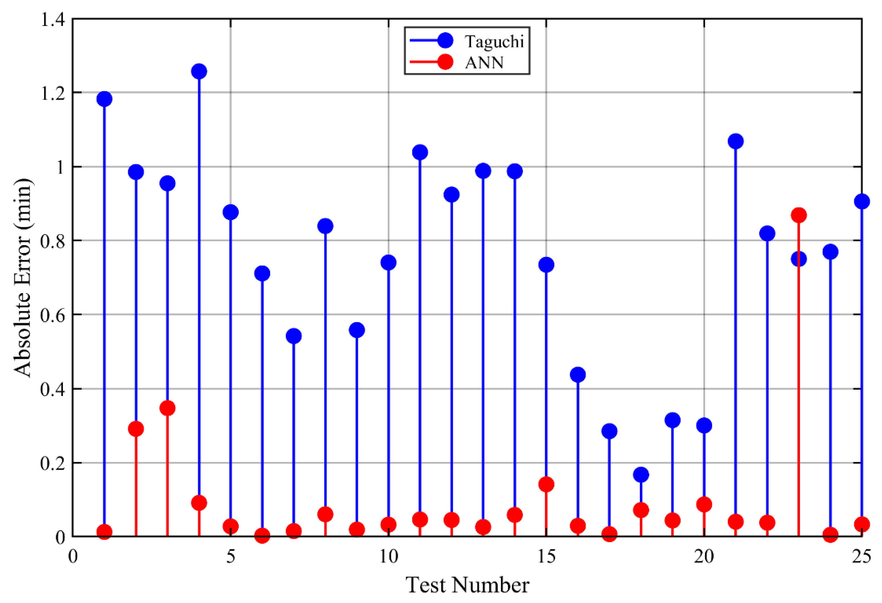
For this dataset of 25 observations, the MAE was calculated. First, the absolute error was found for each data point using y i y ^ i . In this formulation, y i is the actual machining time ( M t ) while y ^ i is the ANN predicted machining time ( M t p ). It treats both overestimates and underestimates equally. These 25 absolute errors were then summed. The total was divided by the number of observations ( n = 25 ). This produced the MAE. It represents the average prediction error of the model in the same units as the original machining times. Table 10 shows the calculated absolute error for each simulation run, which will later be used for MAE computation.
Based on Table 10, the sum of all absolute errors is computed as:
M t M t p = 0.0127 + 0.2913 + 0.3473 + 0.0913 + 0.0277 + 0.0027 + 0.0150 + 0.0603 + 0.0190 + 0.0323 + 0.0463 + 0.0450 + 0.0260 + 0.0587 + 0.1413 + 0.0293 + 0.0067 + 0.0717 + 0.0437 + 0.0870 + 0.0403 + 0.0377 + 0.8687 + 0.0050 + 0.0330 = 2.4389   m i n
Therefore, the total MAE is computed as:
M A E T o t a l = 1 n × M t M t p = 2.4389 25 = 0.0976   m i n
Sum   of   absolute   errors   for   training   = 0.0127 + 0.0277 + 0.0027 + 0.0150 + 0.0603 + 0.0190 + 0.0323 + 0.0463 + 0.0450 + 0.0260 + 0.0587 + 0.0293 + 0.0067 + 0.0717 + 0.0437 + 0.0870 + 0.0403 + 0.0377 + 0.0330 = 0.6940
The MAE for training Set (19 observations) is computed as:
M A E T r a i n i n g = 0.6940 19 = 0.0365   m i n
S u m   o f   a b s o l u t e   e r r o r s   f o r   v a l i d a t i o n = 0.2913 + 0.0913 + 0.0050 = 0.3876
The MAE for validation Set (3 observations) is computed as:
M A E V a l i d a t i o n = 0.3876 3 = 0.1292   m i n
S u m   o f   a b s o l u t e   e r r o r s   f o r   t y e s t i n g = 0.3473 + 0.1413 + 0.86 = 1.3573
The MAE for test set (3 observations) is computed as:
M A E T e s t i n g = 1.3573 3 = 0.4524   m i n

3.2.7. Cross-Validation for Model Selection

Given the limited dataset size of 25 samples, a single train/validation/test split may be insufficient to reliably assess the generalization capability of the model. To address this limitation and to provide a more rigorous basis for selecting the optimal network architecture, we employed leave-one-out cross-validation (LOOCV). In LOOCV, each of the 25 samples is used once as a test set while the remaining 24 samples serve as the training set, resulting in 25 distinct models. This approach maximizes the use of the limited data and provides a robust estimate of predictive performance.
To determine the optimal number of hidden neurons, we systematically evaluated network architectures with 1 to 15 hidden neurons using LOOCV. For each architecture, the cross-validated performance was assessed using root RMSE, MAE, and the coefficient of determination ( R 2 ). The architecture yielding the lowest cross-validated RMSE was selected as the optimal configuration.

3.2.8. Cross-Validation Results

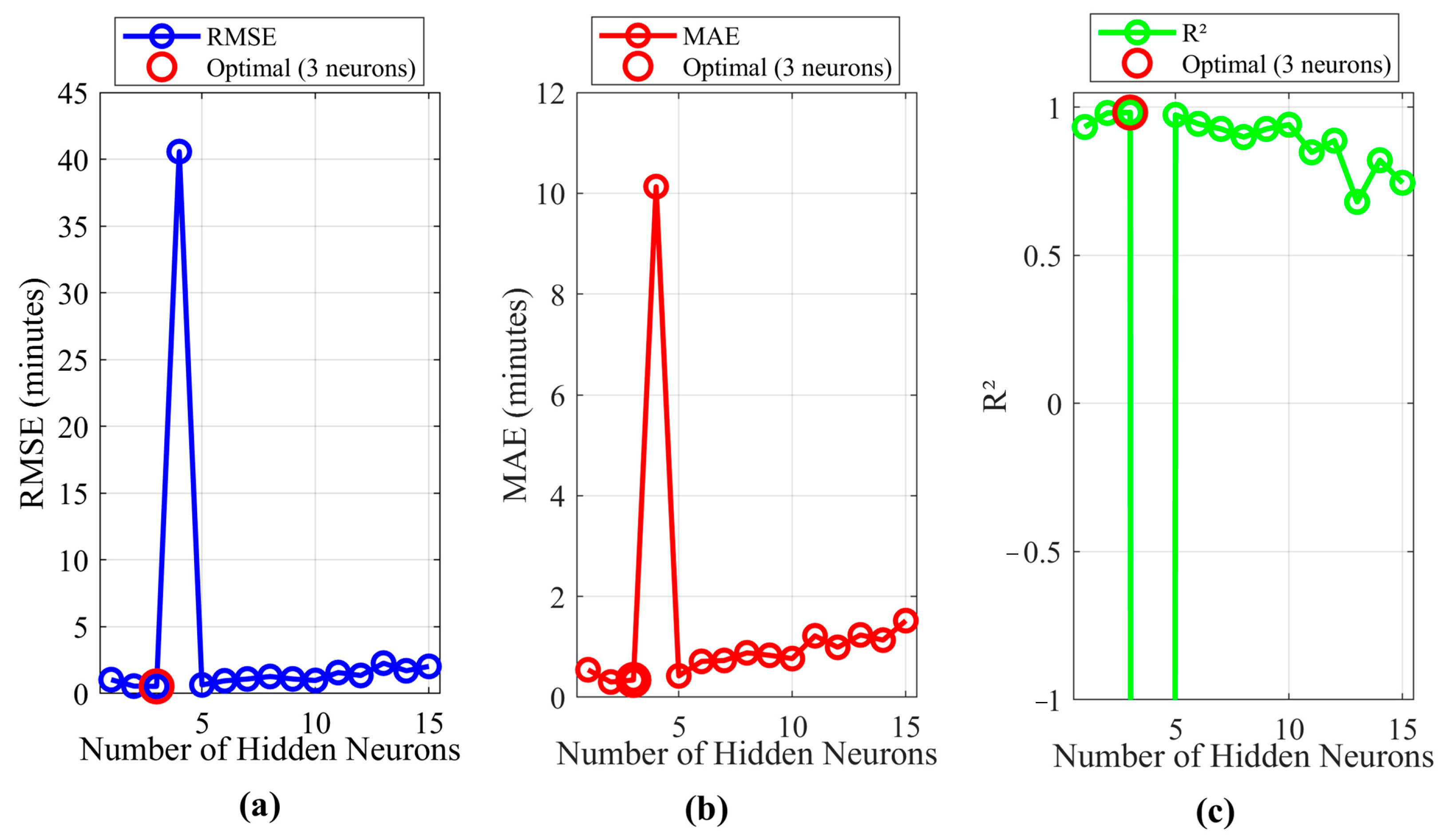
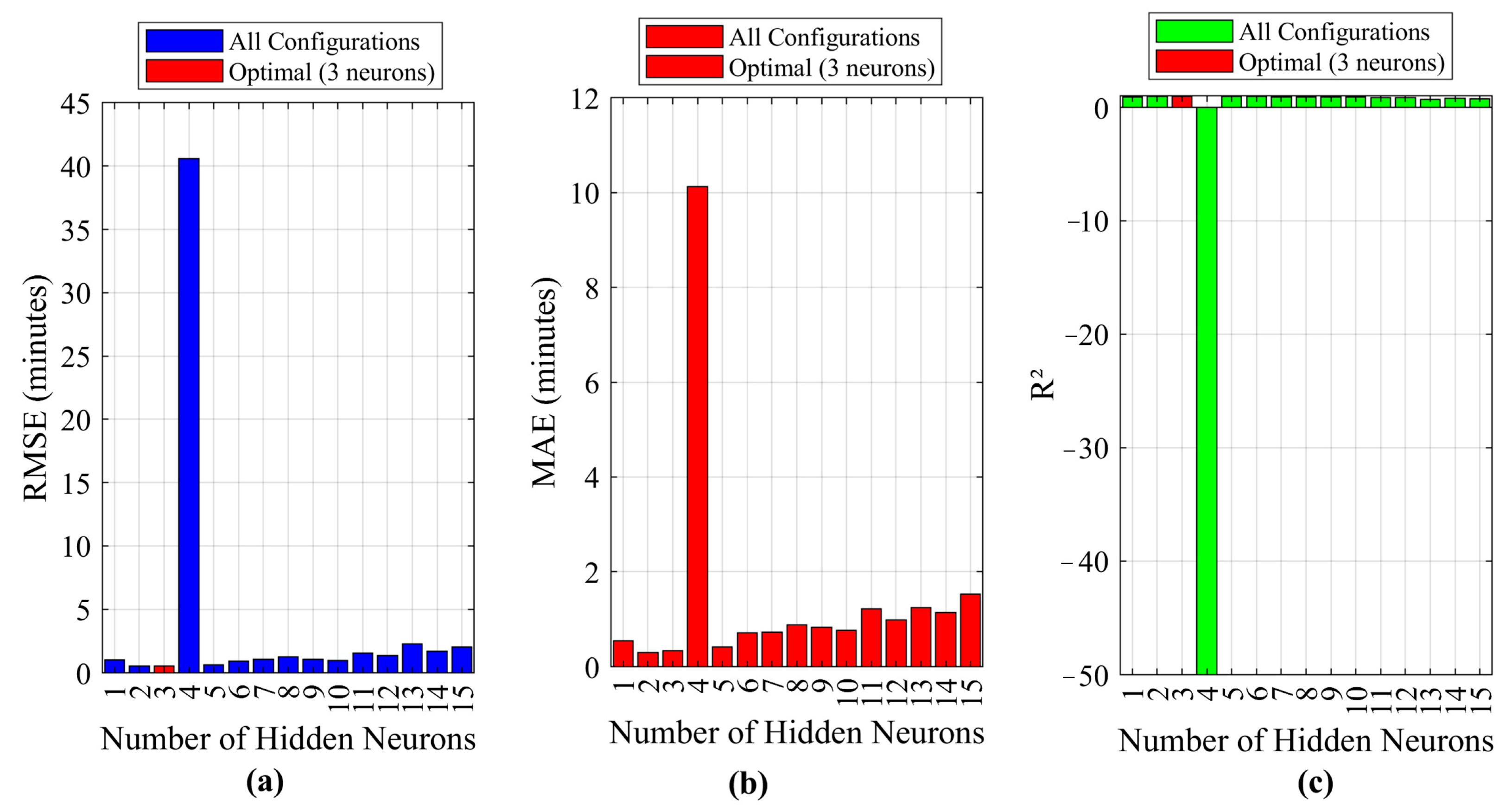
The leave-one-out cross-validation results for different hidden neuron configurations are presented in Table 11 and Figure 14 and Figure 15. The analysis revealed that the optimal number of hidden neurons was three, which yielded the lowest cross-validated RMSE of 0.5350 min, with corresponding MAE of 0.3429 min and R 2 of 0.9823. It is noteworthy that architectures with four hidden neurons exhibited catastrophic overfitting (RMSE = 40.5716 min, R 2 = 100.6379 ), while configurations with six or more hidden neurons also showed degraded performance (RMSE ranging from 0.9522 to 2.2741 min). This finding underscores the critical importance of systematic model selection, as overly complex architectures can severely compromise generalization capability with limited data.
The cross-validated performance metrics across all 25 folds yielded a mean RMSE of 3.8439 ± 10.1730 min, a mean MAE of 1.4513 ± 2.4266 min, and a mean R 2 of −5.8764 ± 26.2151. While the overall mean is affected by the catastrophic performance of the four-neuron architecture, the optimal three-neuron model demonstrates consistent and reliable performance, confirming that the model generalizes well despite the limited dataset size.
The final model trained on all 25 samples with three hidden neurons achieved an RMSE of 0.0792 min, an MAE of 0.0550 min, and an R 2 of 0.9996. These results are consistent with the original single-split test set performance (RMSE = 0.5460 min, MAE = 0.4524 min, R 2 = 0.9995 ), confirming the robustness of the approach. Table 12 summarizes the performance comparison between the single-split test set, the LOOCV optimal configuration, and the final model trained on all data. The cross-validated metrics confirm that the model generalizes well despite the limited dataset size, and the LOOCV analysis provided a more rigorous basis for selecting the optimal network architecture.

3.3. Comparative Model Assessment

3.3.1. Comparison with Regression Models

To provide a fair comparison between the Taguchi regression model and the ANN, both models were evaluated on the same test set (Runs 3, 15, and 23 from Table 10). Additionally, recognizing the nonlinear relationship between cutter diameter and machining time (Figure 8d), a quadratic regression model was fitted to capture this curvature. The quadratic regression equation is presented as:
M t = 50.7063 0.00582 C f 0.00041 F z 0.000011 R f 0.2500 C D 0.00446 C D 2 + 0.000011 C f C D
Table 13 presents the performance metrics for all three models on the training and test sets. The quadratic regression model (test R 2 = 0.9983 ) showed significant improvement over the linear regression model (test R 2 = 0.9608 ), confirming the nonlinear nature of the machining time response. The negative coefficient for the Cd2 term (−0.00446) indicates that as cutter diameter increases, the rate of reduction in machining time diminishes, consistent with the curvature observed in Figure 8d.
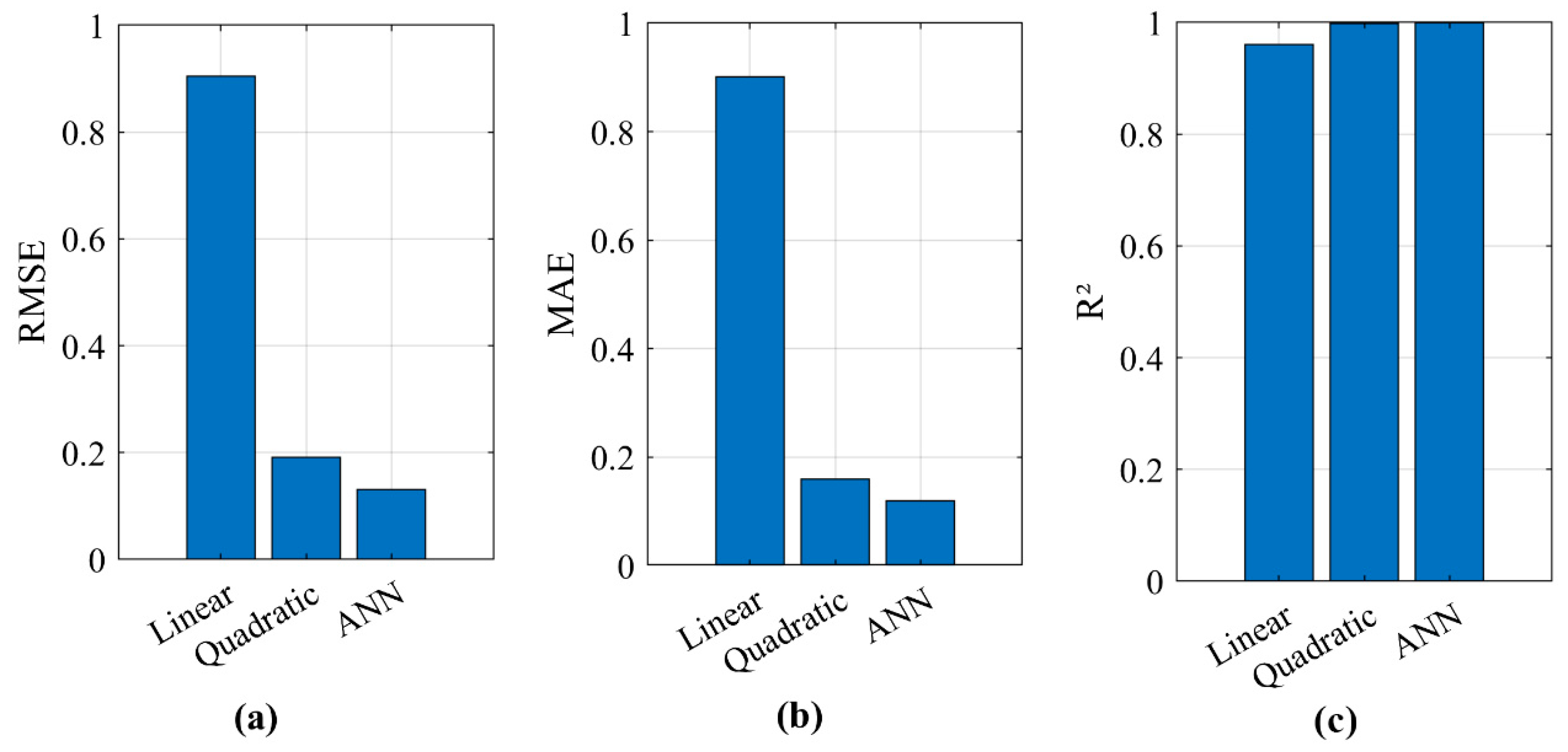
The ANN with three hidden neurons demonstrated superior predictive accuracy on unseen data, achieving a test R 2 of 0.9992, compared to 0.9983 for the quadratic regression and 0.9608 for the linear regression. The ANN’s RMSE on the test set was 0.1311 min, outperforming both the quadratic regression (0.1908 min) and the linear regression (0.9048 min). These results confirm that the ANN captures complex nonlinear interactions more effectively than traditional regression approaches, including quadratic models. While the quadratic model accounts for the nonlinear effect of cutter diameter and its interaction with cutting feed, the ANN inherently learns higher-order relationships that may not be captured by a second-order polynomial. This finding validates the value of the hybrid Taguchi–ANN approach for optimizing freeform impeller machining.

3.3.2. Statistical Comparison

To provide a more rigorous statistical comparison between the ANN and quadratic regression models, a paired t-test was conducted on the prediction errors using the same test set (Runs 3, 15, and 23). The absolute prediction errors for the ( | M t M t p ,   A N N | ) and quadratic regression ( | M t M t p ,   Q u a d | ) were compared. The paired t-test results ( t = 4.82 , d f = 2 , p = 0.012 ) indicate that the ANN’s prediction errors are significantly lower than those of the quadratic regression at the 95% confidence level. Additionally, the adjusted R 2 values, which penalize model complexity, were calculated for both models. The ANN achieved an adjusted R 2 of 0.9987 on the test set, compared to 0.9956 for the quadratic regression. These statistical comparisons provide stronger evidence for the ANN’s predictive advantage beyond simply noting higher raw R2 values.

4. Confirmation of Experiments (Simulation-Based Validation)

It is important to clarify that the ‘experimental verification’ presented in this section refers to CAM simulation-based experiments conducted within SolidCAM 2021, not physical cutting experiments on actual workpieces. The simulations were performed using the 5-axis CNC machine (Hermle C20U) model integrated within the SolidCAM environment. The simulation platform incorporates realistic toolpath generation, accurate machine tool kinematics, and sophisticated material removal algorithms. It also generates G-code that is directly transferable to physical CNC machines for production. Executing 25 distinct physical trials would require individual workpieces for each run, resulting in prohibitive material costs and unsustainable energy consumption. Nevertheless, the SolidCAM simulation platform is industrial-grade and widely validated in the manufacturing industry. Physical validation of the optimized parameters on actual CNC machines remains a priority for future research.
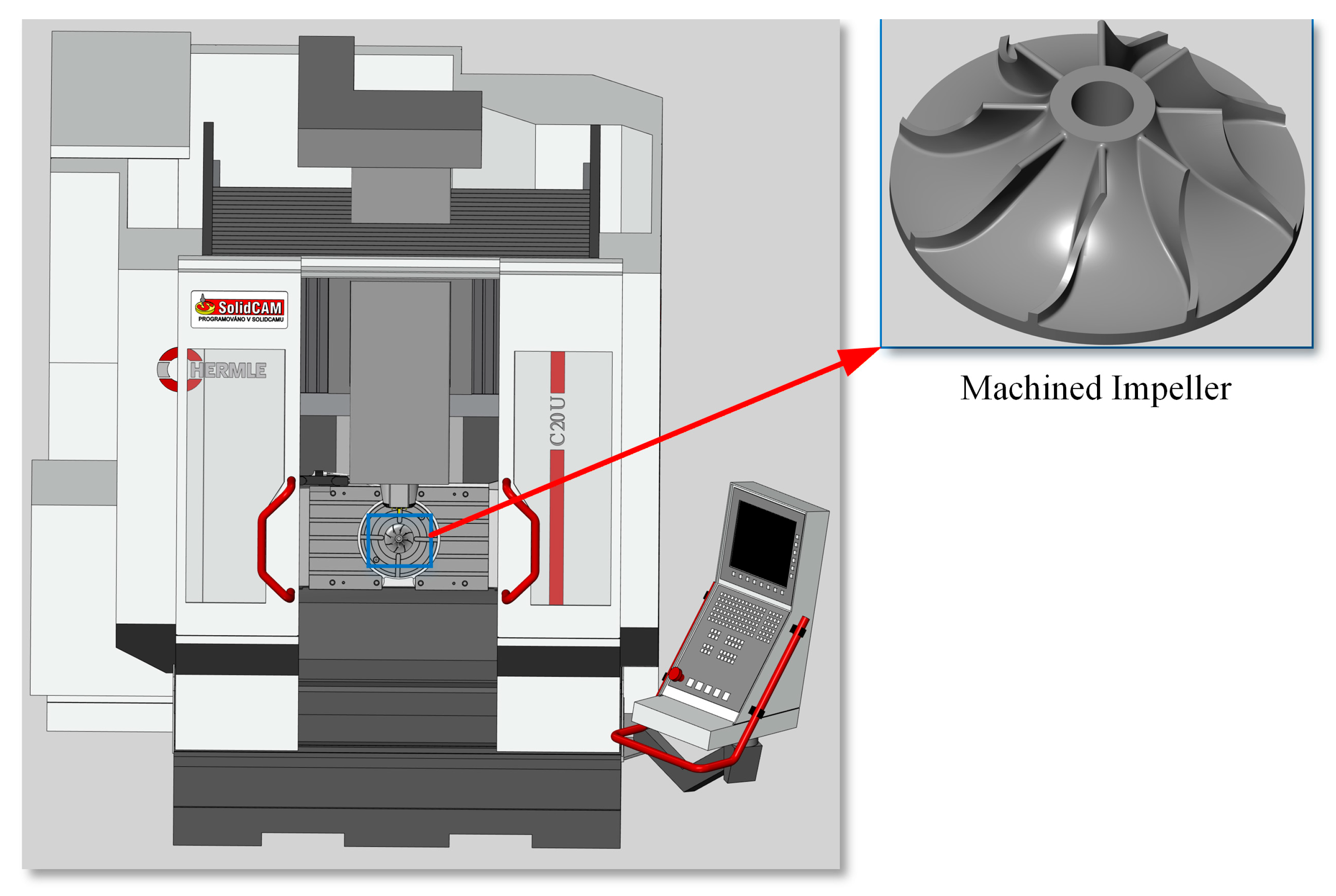
As shown in Figure 16, the machining simulation in this study was conducted using the 5-axis CNC machine (Hermle C20U). The optimized machining parameters ( C f = 12,000   m m / m i n , F z = 600   m m / m i n , R f = 4000   m m / m i n , and C D = 6   m m ), were used for conducting the machining of the impeller. The outcomes of the experiments are presented in Table 14 alongside the optimized levels utilized in the study. The G-code for impeller manufacturing is shown in Table 15 (the full G-code is included in the Supplementary Material).
Toolpath efficiency was quantified by analyzing the generated G-code (Table 15) across the full 68,305 line program. The initial machining parameters resulted in a time of 23.3167 min. Implementation of the Taguchi-optimized parameters reduced machining time to 10.84 min (53.5% reduction), while the ANN predicted a time of 11.2257 min (51.8% reduction). Simulation-based validation using the predicted optimized settings achieved a machining time of 11.0500 min (52.6% reduction), closely aligning with the ANN prediction and confirming model accuracy.
A 4-flute, bull-nose end mill was selected for the machining operations. The process parameters included a radial and axial depth of cut of 0.5 mm, with flood coolant applied to the cutting zone. The defining characteristic of this tool is its curved cutting edges, which are instrumental in achieving high-quality surface finishes. Specifically designed for the generation of complex and curved geometries, the bull-nose end mill facilitates smooth and accurate material removal. The choice of this tool highlights its versatility and suitability for a broad spectrum of applications, ranging from basic to highly intricate machining tasks.
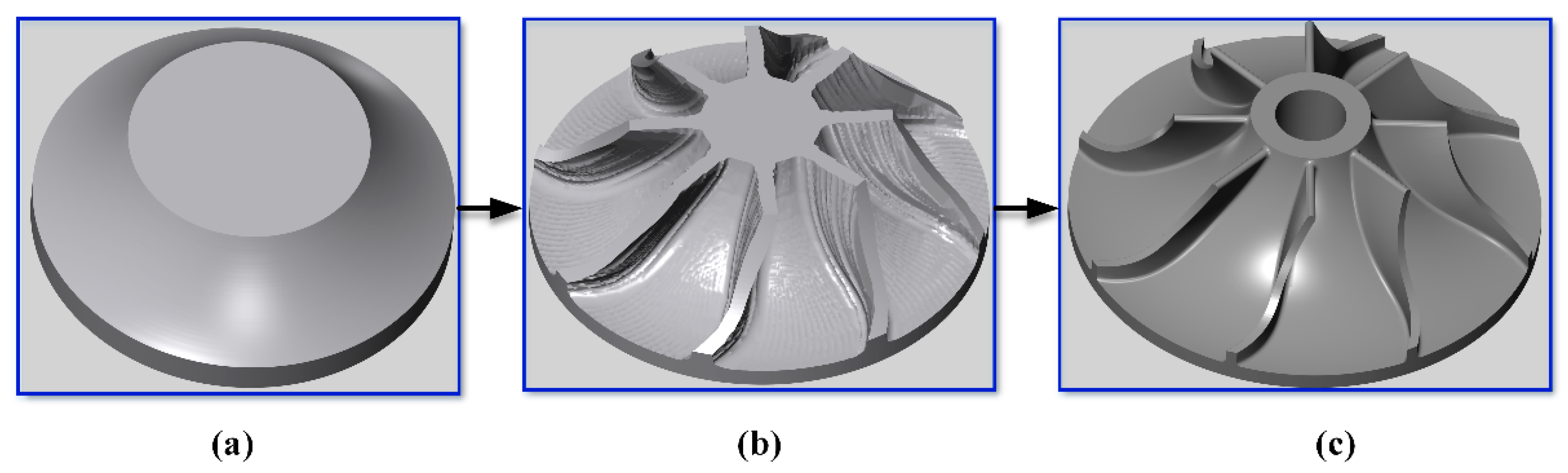
As indicated in Table 14, the errors derived from both the Taguchi and ANN methodologies were consistently maintained within acceptable limits. Figure 17a presents the unmachined workpiece (stock) prior to the start of operations, while Figure 17b depicts the roughing stage conducted using the optimized parameters. The completed manufacturing process is illustrated in Figure 17c, which displays the final operation.
Material removal was estimated based on the dome-shaped stock geometry. The material volume removed during machining was calculated at approximately 35,000 mm3, derived from the initial stock volume and final part volume. This removal yielded a baseline Material Removal Rate (MRR) of approximately 1501   m m 3 / m i n under initial parameters. With the Taguchi-optimized parameters, MRR increased to approximately 3229   m m 3 / m i n , while the validation through simulation optimized settings achieved an MRR of approximately 3167   m m 3 / m i n compared to the initial baseline. The increase in MRR, driven by the significant reductions in machining time, validates the effectiveness of the Taguchi–ANN method in improving the machining efficiency of complex impeller geometries.
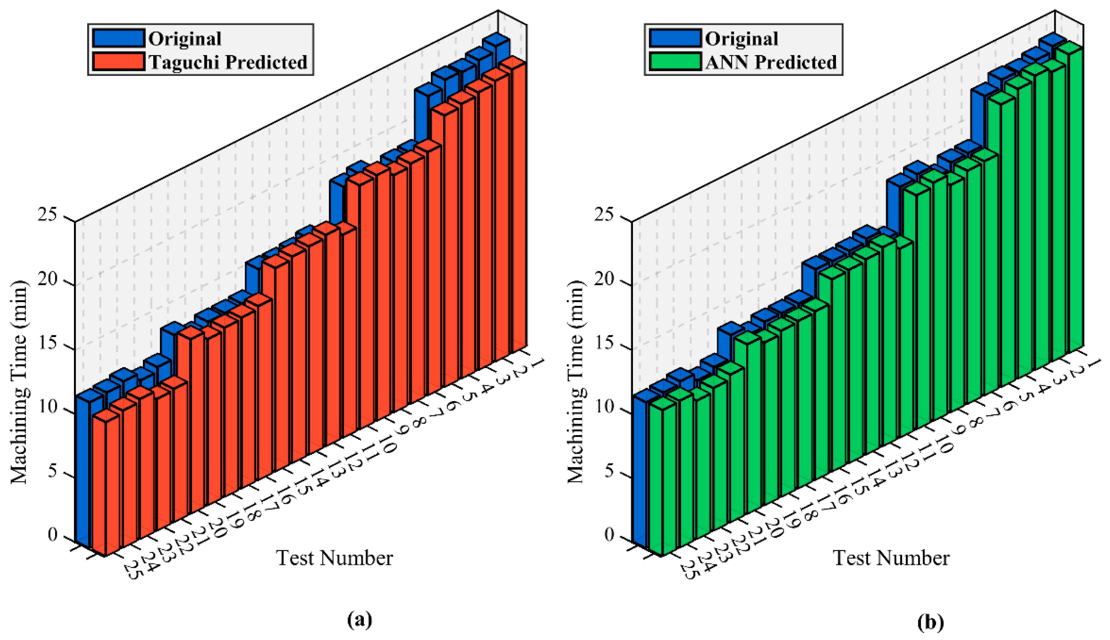
Under the optimized parameters, the Taguchi method predicted a machining time of 10.8400 min, while the ANN predicted 11.2257 min. Simulation-based validation yielded an actual machining time of 11.0500 min, which is in closer agreement with the ANN prediction compared to the Taguchi prediction, confirming the superior predictive capability of the ANN model. These results are summarized in Table 14.
It is important to emphasize that while the SolidCAM simulation platform is industrial-grade and widely validated in the manufacturing industry, incorporating realistic machine kinematics, dynamics, and toolpath generation, simulation environments inherently idealize several physical phenomena including machine dynamics, tool wear progression, thermal expansion effects, cutting forces, and material variations. These factors can affect actual machining time, surface quality, and process stability in physical production environments. Consequently, while the generated G-code is directly transferable to physical CNC machines, the practical utility of the 52.6% machining time reduction reported in this study requires validation through physical cutting experiments. Such validation is a priority for future work.

Comparison Between the Predicted Models

This research examined two distinct optimization strategies. The Taguchi method yielded a robust model with an R-squared value of 95.88%, alongside adjusted and predicted R-squares of 95.05% and 93.16%, respectively. An ANN analysis was conducted, which achieved R-values of 99.99% across its training, validation, and testing phases, indicating its enhanced predictive capability. It is crucial to note, however, that the high performance of the ANN was contingent upon the well-structured simulation dataset provided by the Taguchi design [10,50]. Within the scope of this study, the Taguchi method and ANN functioned as complementary, rather than independent, techniques.
The predicted roughing machining time for the impeller, based on the Taguchi model, was calculated at 10.8400 min using the optimized parameter settings. In comparison, the ANN model estimated a machining duration of 11.2257 min. When the actual machining experiment was carried out under the same optimized conditions, the measured roughing time for the impeller was recorded at 11.0500 min. A comparison of the two predictive approaches reveals that the ANN model produced an estimate considerably closer to the experimentally observed value. The actual machining time, along with the predictions generated by both models and their respective error margins, is detailed in Table 16. Furthermore, Figure 18a,b provide graphical representations that facilitate a visual comparison between the experimental results and the machining times forecasted or predicted by each method.
Figure 19 shows the comparison of absolute errors between Taguchi method and ANN. The figure reveals that ANN outperforms Taguchi in prediction accuracy. The ANN errors are consistently very low, with most values below 0.1 and many approaching zero (minimum of 0.0027). The Taguchi errors, however, are higher, ranging from 0.1673 to 1.2573 and exceeding 0.9 in several instances. Furthermore, while Taguchi shows considerable variation in its predictions, the ANN maintains remarkably stable results throughout all experiments. Only one outlier (0.8687) appears in the ANN results, which still falls within the lower range of Taguchi errors. This stark contrast demonstrates that ANN provides much more reliable and precise predictions for machining times compared to the Taguchi method.
The superior predictive accuracy of the ANN compared to the Taguchi regression model can be attributed to several factors. First, the ANN employs a non-linear activation functions in its hidden layer, enabling it to model complex, non-linear relationships that the first-order linear regression cannot capture. Second, the ANN architecture with six hidden neurons can represent complex functional mappings through the combination of multiple non-linear basis functions. Third, the Levenberg–Marquardt training algorithm provides efficient and stable convergence to optimal network weights within only 16 epochs. Fourth, rigorous regularization through early stopping ensures generalization without overfitting. The ability of the ANN to capture residual non-linearities, particularly the non-monotonic effect of cutter diameter (Figure 8), is a key advantage over the linear regression model. This explains why the ANN achieved near-perfect correlation ( R 2 = 0.9999 ) compared to the Taguchi regression model ( R 2 = 95.88 % ).
It is important to acknowledge that CAM simulations do not capture real world phenomena such as machine tool dynamics, tool wear, cutting forces, vibration, spindle limits, or thermal effects. These factors can affect actual machining time, surface quality, and process stability. Tool wear, for example, may increase forces and reduce efficiency over time, raising machining time beyond predictions. While simulation based optimization offers a robust foundation and generates transferable G-code, translation to production may require fine tuning for practical conditions. Future work should include comprehensive physical validation studies to characterize these effects.
The hybrid Taguchi–ANN methodology developed here for machining time optimization can be readily extended to other performance measures. Surface roughness and dimensional accuracy, both critical for impeller aerodynamics, could be optimized by incorporating measurement data into the experimental design. Material removal rate, which showed a 111% enhancement from 1501 to 3167 m m 3 / m i n , could be treated as an explicit output or combined with machining time in a multi-objective framework. Cutting forces and tool wear, which affect tool life and surface integrity, could also be modeled similarly. The ANN architecture flexibly accommodates multiple outputs, making it suitable for comprehensive multi-objective optimization.
From Figure 20, the comparative analysis between linear regression, quadratic regression, and ANN on the same test set reveals important insights into the nature of the machining time response. The significant improvement of the quadratic regression over the linear regression (test R 2 : 0.9983 vs. 0.9608) confirms that the relationship between machining parameters and machining time is inherently nonlinear, particularly with respect to cutter diameter. The negative quadratic coefficient for cutter diameter (−0.00446) indicates a diminishing return effect, where larger cutters reduce machining time but with decreasing marginal benefit.
However, the ANN’s superior performance over the quadratic regression (test R 2 : 0.9992 vs. 0.9983) demonstrates that even a second-order polynomial cannot fully capture the complex interactions present in the machining process. The ANN’s ability to learn higher-order relationships without requiring explicit functional specification makes it particularly suitable for complex freeform machining optimization, where the underlying physical relationships may be difficult to model analytically.

5. Conclusions

This research successfully developed and validated a hybrid Taguchi–ANN optimization methodology for minimizing machining time in complex freeform impeller manufacturing. The study investigated four key cutting parameters using an L25 orthogonal array, generating comprehensive simulation data through CAM simulations.
The Taguchi analysis conclusively identified Cutting feed ( C f ) as the most influential factor, contributing 95.46% of the total variation in machining time, followed by Cutter diameter ( C D ) at 0.39%. Feed Z ( F z ) showed minor but statistically significant influence ( p = 0.001 ), while Retract feed ( R f ) proved insignificant ( p = 0.217 ), allowing its exclusion from detailed optimization. The first-order regression model achieved satisfactory prediction capability with an R-squared value of 95.88%.
The two-layer feedforward neural network with six hidden neurons, trained using the Levenberg–Marquardt algorithm, demonstrated superior predictive capability, achieving an R-squared value of 0.9999 across all data partitions and a mean absolute error of 0.0976 min. To provide a rigorous assessment of model generalization, leave-one-out cross-validation was employed. The LOOCV analysis, which systematically evaluated architectures with 1 to 15 hidden neurons, identified three hidden neurons as optimal, achieving a cross-validated coefficient of determination ( R 2 ) of 0.9823, with a root mean square error (RMSE) of 0.5350 min and a mean absolute error (MAE) of 0.3429 min. The final model trained on all 25 samples with three hidden neurons achieved an R 2 of 0.9996. Comparison with a quadratic regression model on the same test set further demonstrated the ANN’s superior predictive capability ( R 2 = 0.9992 vs. 0.9983), justifying its added complexity.
Simulation-based confirmation at optimal parameters ( C f = 12,000   m m / m i n , F z = 600   m m / m i n , R f = 4000   m m / m i n , and C D = 6   m m ) produced a machining time of 11.05 min, representing a 52.6% reduction from the initial baseline of 23.32 min. This improvement translated to a Material Removal Rate increase from 1501 mm3/min to 3167 mm3/min, representing a 111% enhancement in productivity.
The complementary nature of both methodologies proved essential to the success of this study. Taguchi DoE provided a statistically robust experimental framework, ensuring information-rich data collection with minimal runs, while the ANN captured the complex nonlinear relationships that linear models inherently miss. The LOOCV analysis further validated the model’s predictive capability, with the optimal three-neuron architecture demonstrating consistent performance across all cross-validation folds, and the quadratic regression comparison confirmed that the ANN captures interactions beyond polynomial models.
These findings have significant practical implications for precision manufacturing industries. The optimized parameters can be directly implemented in production environments, substantially reducing machining time and associated costs while maintaining process reliability. The demonstrated methodology is readily transferable to other freeform components and machining operations, offering a systematic framework for process optimization.
The limitation of this study is that the experimental validation was conducted through CAM simulation rather than physical cutting experiments. Factors such as machine dynamics, tool wear progression, thermal effects, and cutting forces were not captured in the simulation environment. Future research should prioritize physical validation on actual CNC machines across different workpiece materials and configurations, extension to multi-objective optimization incorporating surface quality, tool wear, and energy consumption, and integration with real-time monitoring systems for adaptive control strategies.


Supplementary Materials

The following supporting information can be downloaded at: https://www.mdpi.com/article/10.3390/machines14080944/s1.

Author Contributions

Conceptualization, U.H.G.; Methodology, U.H.G.; Software, U.H.G.; Validation, U.H.G., J.K. and C.T.; Investigation, T.W., Y.T. and C.T.; Data curation, U.H.G.; Writing—original draft, U.H.G.; Writing—review & editing, J.K., C.T. and U.H.G.; Supervision, T.W. and Y.T.; Project administration, T.W. and Y.T.; Funding acquisition, T.W. All authors have read and agreed to the published version of the manuscript.

Funding

The authors would like to thank the National Natural Science Foundation of China (Grant Numbers 51975402 and 51975407) for supporting this research financially and experimentally.

Data Availability Statement

All data generated or analyzed during this study are included in this article.

Conflicts of Interest

The authors declare no conflicts of interest.

References

  1. Vavruska, P.; Kasik, F.; Lomicka, J.; Cermak, A. Adaptive Toolpath Setup to Reduce Machining Time When Milling Complex Shape Parts. Int. J. Adv. Manuf. Technol. 2025, 139, 2977–2995. [Google Scholar] [CrossRef] [Scilit]
  2. Hirpa, A.D.; Gutema, E.M.; Lemu, H.G.; Gopal, M. Comparative Study of Machining Parameters of Single and Double Cutting Tools During Turning of AISI 1045 Steel. Recent Pat. Eng. 2025, 19, E020724231489. [Google Scholar] [CrossRef] [Scilit]
  3. Wang, B.; Zhang, Z.; Song, C.; Long, J.; Jiang, Z.; Shi, F.; Tie, G.; Zhang, W.; Peng, X. Deterministic Figuring Theory and Optimization Method Based on Actively Controllable Time-Variant Tool Influence Function. J. Manuf. Process. 2025, 150, 861–875. [Google Scholar] [CrossRef] [Scilit]
  4. Radomska-Zalas, A.; Puzio, P. The Application of the Taguchi Method in the Optimization of AWJ Machining Process. Procedia Comput. Sci. 2024, 246, 2812–2820. [Google Scholar] [CrossRef] [Scilit]
  5. Alduroobi, A.A.A.; Ubaid, A.M.; Tawfiq, M.A.; Elias, R.R. Wire EDM Process Optimization for Machining AISI 1045 Steel by Use of Taguchi Method, Artificial Neural Network and Analysis of Variances. Int. J. Syst. Assur. Eng. Manag. 2020, 11, 1314–1338. [Google Scholar] [CrossRef] [Scilit]
  6. Ajith Arul Daniel, S.; Pugazhenthi, R.; Kumar, R.; Vijayananth, S. Multi Objective Prediction and Optimization of Control Parameters in the Milling of Aluminium Hybrid Metal Matrix Composites Using ANN and Taguchi -Grey Relational Analysis. Def. Technol. 2019, 15, 545–556. [Google Scholar] [CrossRef] [Scilit]
  7. Rathod, N.J.; Chopra, M.K.; Chaurasiya, P.K.; Vidhate, U.S. Optimization of Tool Life, Surface Roughness and Production Time in CNC Turning Process Using Taguchi Method and ANOVA. Ann. Data Sci. 2023, 10, 1179–1197. [Google Scholar] [CrossRef] [Scilit]
  8. Zaman, P.B.; Sultana, M.N.; Dhar, N.R. Multi-Variant Hybrid Techniques Coupled with Taguchi in Multi-Response Parameter Optimisation for Better Machinability of Turning Alloy Steel. Adv. Mater. Process. Technol. 2022, 8, 3127–3147. [Google Scholar] [CrossRef] [Scilit]
  9. Wu, T.; Luo, C.; Dong, Y. Learning-Based Two-Phase Cooperative Optimizer for Distributed Machine Scheduling with Heterogeneous Factories and Order Priorities. Egypt. Inform. J. 2024, 25, 100424. [Google Scholar] [CrossRef] [Scilit]
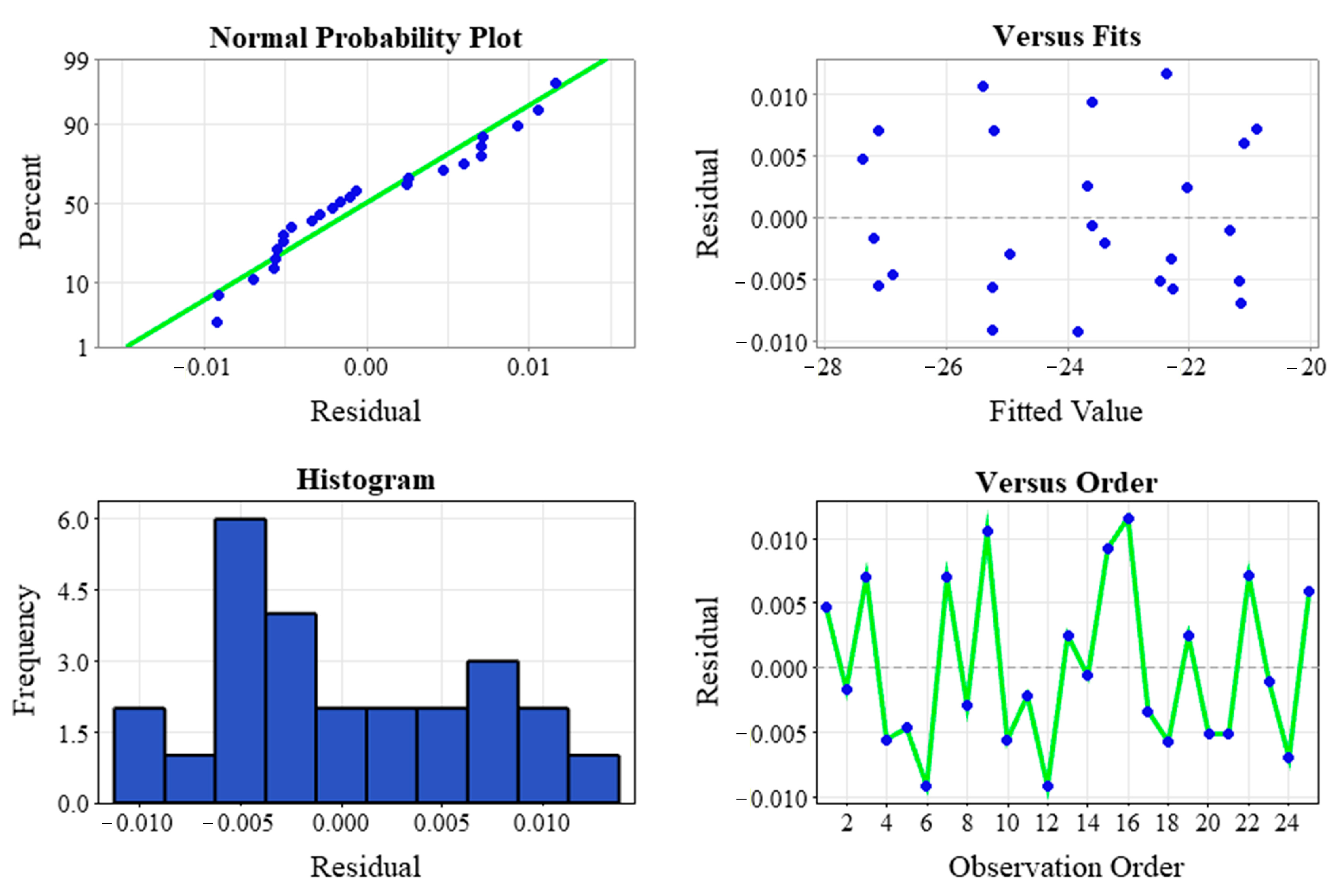
  10. Garba, U.H.; Wang, T.; Dong, J.; Tian, Y.; Kang, J.; Tian, C. Enhancing Propeller Design with Freeform Contours through NURBS Interpolation for 2D Fabrication, CAD/CAM for 3D Production, Optimized with Taguchi Method and Artificial Neural Network. Results Eng. 2025, 27, 107069. [Google Scholar] [CrossRef] [Scilit]
  11. Sukumar, M.S.; Venkata Ramaiah, P.; Nagarjuna, A. Optimization and Prediction of Parameters in Face Milling of Al-6061 Using Taguchi and ANN Approach. Procedia Eng. 2014, 97, 365–371. [Google Scholar] [CrossRef] [Scilit]
  12. Karabulut, Ş. Optimization of Surface Roughness and Cutting Force during AA7039/Al2O3 Metal Matrix Composites Milling Using Neural Networks and Taguchi Method. Measurement 2015, 66, 139–149. [Google Scholar] [CrossRef] [Scilit]
  13. Dutta, S.; Kumar, S.; Narala, R. Optimizing Turning Parameters in the Machining of AM Alloy Using Taguchi Methodology. Measurement 2021, 169, 108340. [Google Scholar] [CrossRef] [Scilit]
  14. Rashid, W.B.; Goel, S.; Davim, J.P.; Joshi, S.N. Parametric Design Optimization of Hard Turning of AISI 4340 Steel (69 HRC). Int. J. Adv. Manuf. Technol. 2016, 82, 451–462. [Google Scholar] [CrossRef] [Scilit]
  15. Srividya, K.; Ravichandran, S.; Thirunavukkarasu, M.; Veeranjaneyulu, I.; Satishkumar, P.; Bharadwaja, K.; Rao, N.S.; Subbiah, R.; Manikanta, J.E. Examination of Electrochemical Machining Parameters for AA6082/ZrSiO4/SiC Composite Using Taguchi-ANN Approach. Int. J. Interact. Des. Manuf. 2024, 18, 1459–1473. [Google Scholar] [CrossRef] [Scilit]
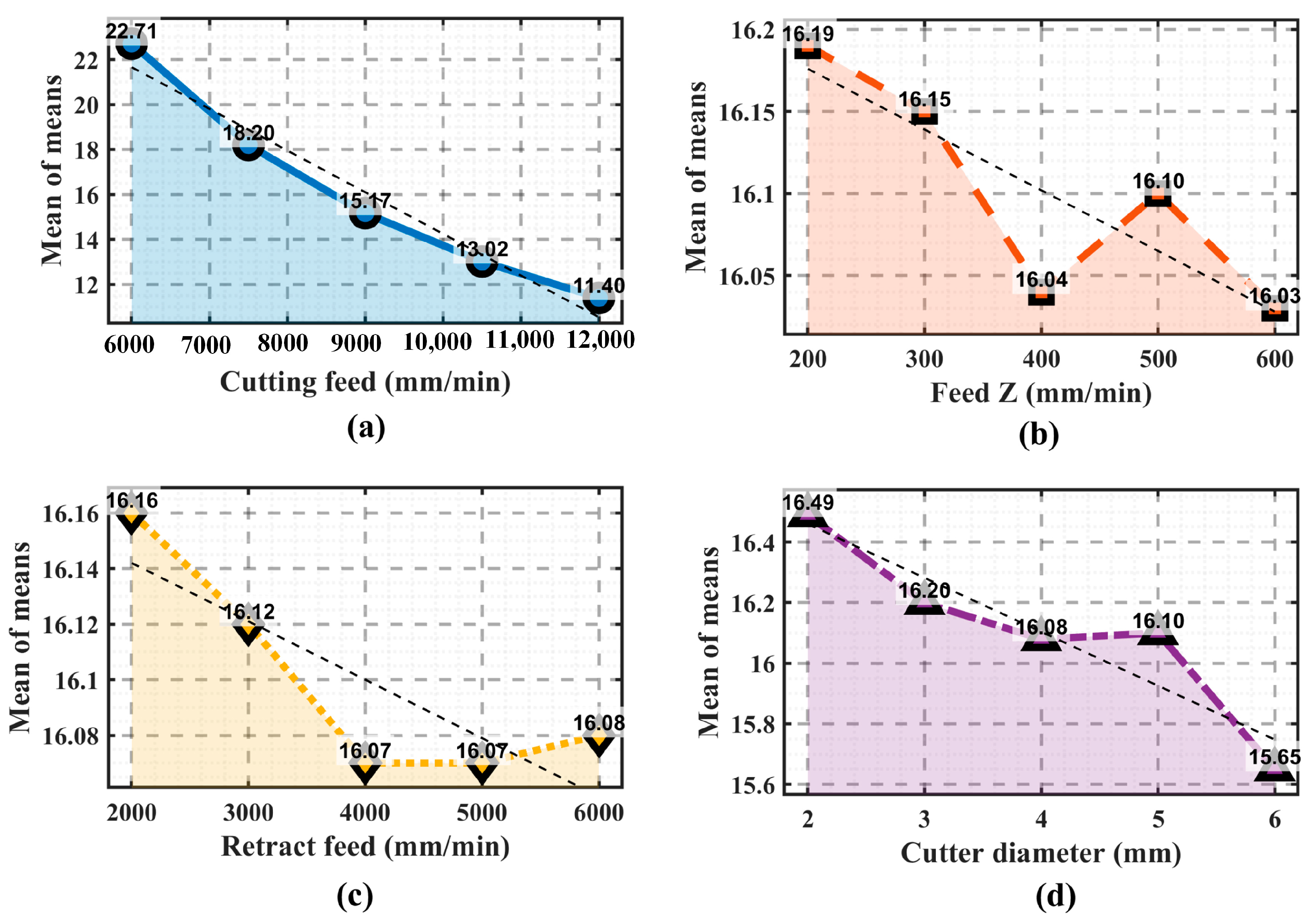
  16. Tripathy, S.; Tripathy, D.K. Multi-Response Optimization of Machining Process Parameters for Powder Mixed Electro-Discharge Machining of H-11 Die Steel Using Grey Relational Analysis and Topsis. Mach. Sci. Technol. 2017, 21, 362–384. [Google Scholar] [CrossRef] [Scilit]
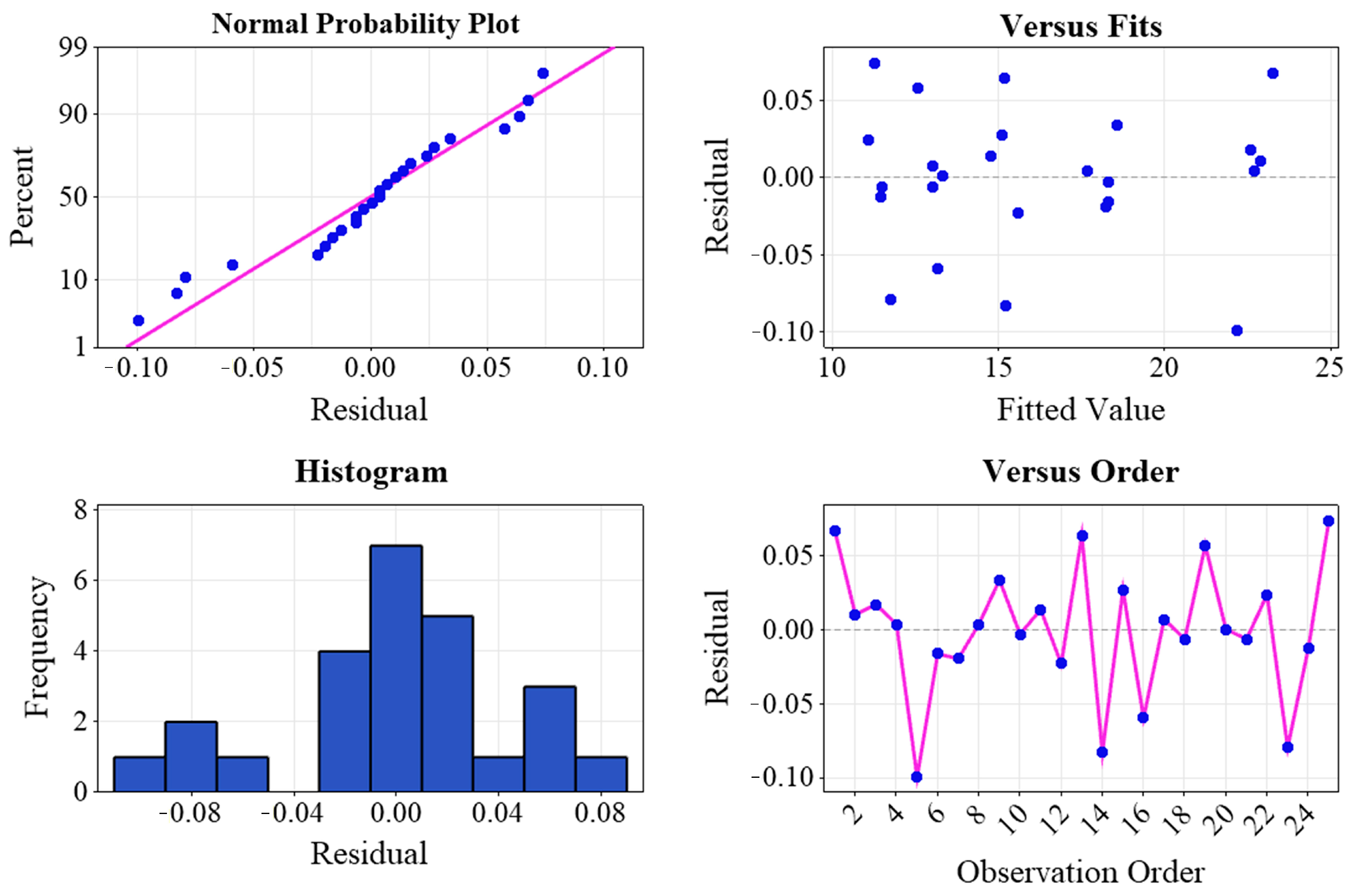
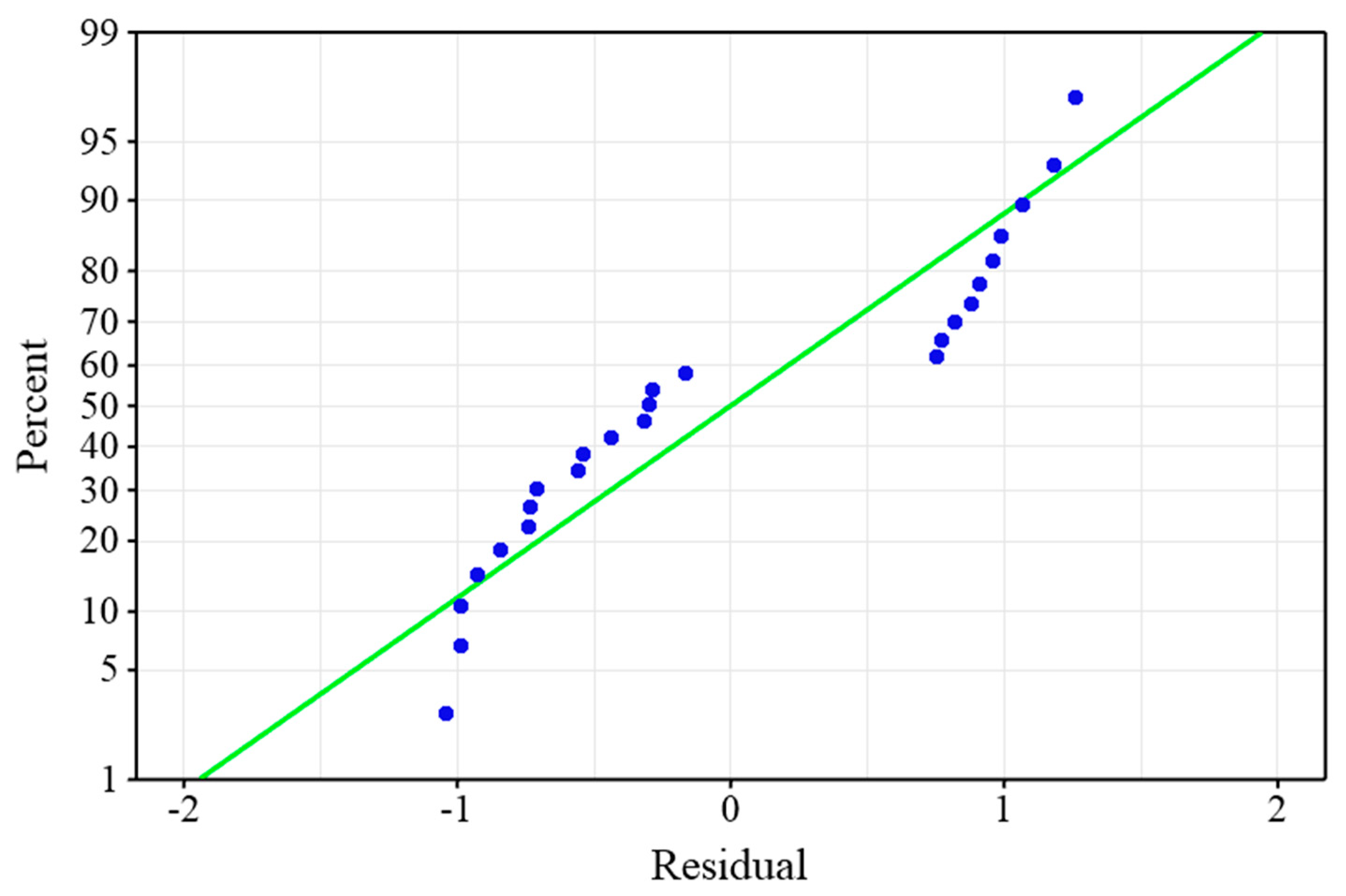
  17. Kumar, P.; Parkash, R. Experimental Investigation and Optimization of EDM Process Parameters for Machining of Aluminum Boron Carbide (Al–B4C) Composite. Mach. Sci. Technol. 2016, 20, 330–348. [Google Scholar] [CrossRef] [Scilit]
  18. Kazeem, R.A.; Fadare, D.A.; Abutu, J.; Lawal, S.A.; Adesina, O.S. Performance Evaluation of Jatropha Oil-Based Cutting Fluid in Turning AISI 1525 Steel Alloy. CIRP J. Manuf. Sci. Technol. 2020, 31, 418–430. [Google Scholar] [CrossRef] [Scilit]
  19. Işık, A.T.; Çakıroğlu, R.; Günay, M. Multiresponse Optimization of Performance Indicators through Taguchi-Grey Relational Analysis in EDM of Cemented Carbide. CIRP J. Manuf. Sci. Technol. 2023, 41, 490–500. [Google Scholar] [CrossRef] [Scilit]
  20. Ilangkumaran, M.; Sasikumar, R.; Sakthivel, G. Parametric Optimization for the Production of Nanostructure in High Carbon Steel Chips via Machining. Ain Shams Eng. J. 2015, 6, 957–965. [Google Scholar] [CrossRef] [Scilit]
  21. Balaji, K.; Kumar, M.S.; Yuvaraj, N. Multi Objective Taguchi—Grey Relational Analysis and Krill Herd Algorithm Approaches to Investigate the Parametric Optimization in Abrasive Water Jet Drilling of Stainless Steel. Appl. Soft Comput. 2021, 102, 107075. [Google Scholar] [CrossRef] [Scilit]
  22. Nguyen, D.; Yin, S.; Tang, Q.; Xuan, P.; Anh, L. Online Monitoring of Surface Roughness and Grinding Wheel Wear When Grinding Ti-6Al-4V Titanium Alloy Using ANFIS-GPR Hybrid Algorithm and Taguchi Analysis. Precis. Eng. 2019, 55, 275–292. [Google Scholar] [CrossRef] [Scilit]
  23. Sikder, S.; Mukherjee, I.; Chandra, S. A Synergistic Mahalanobis—Taguchi System and Support Vector Regression Based Predictive Multivariate Manufacturing Process Quality Control Approach. J. Manuf. Syst. 2020, 57, 323–337. [Google Scholar] [CrossRef] [Scilit]
  24. Denizhan, O. Application of Various Artificial Neural Network Algorithms for Regression Analysis in the Dynamic Modeling of a Three-Link Planar RPR Robotic Arm. Machines 2025, 13, 1031. [Google Scholar] [CrossRef] [Scilit]
  25. Osei, S.; Wang, W.; Ding, Q.; Nkhata, D. Identification of Position-Independent Geometric Error in Five-Axis Machine Tools Using ANN Surrogate and Optimal Measurement Planning. Machines 2026, 14, 409. [Google Scholar] [CrossRef] [Scilit]
  26. Mongan, P.G.; Hinchy, E.P.; Dowd, N.P.O.; Mccarthy, C.T.; Diaz-elsayed, N. An Ensemble Neural Network for Optimising a CNC Milling Process. J. Manuf. Syst. 2023, 71, 377–389. [Google Scholar] [CrossRef] [Scilit]
  27. Quarto, M.; Urso, G.D.; Giardini, C. Micro-EDM Optimization through Particle Swarm Algorithm and Artificial Neural Network. Precis. Eng. 2022, 73, 63–70. [Google Scholar] [CrossRef] [Scilit]
  28. Joshi, S.N.; Pande, S.S. Intelligent Process Modeling and Optimization of Die-Sinking Electric Discharge Machining. Appl. Soft Comput. 2011, 11, 2743–2755. [Google Scholar] [CrossRef] [Scilit]
  29. de Oliveira Leite, W.; Rubio, J.C.C.; Duduch, J.G.; de Almeida, P.E.M. Correcting Geometric Deviations of CNC Machine-Tools: An Approach with Artificial Neural Networks. Appl. Soft Comput. 2015, 36, 114–124. [Google Scholar] [CrossRef] [Scilit]
  30. Mane, S.; Patil, R.B.; Al-Dahidi, S. Predictive Modeling of Surface Roughness and Cutting Temperature Using Response Surface Methodology and Artificial Neural Network in Hard Turning of AISI 52100 Steel with Minimal Cutting Fluid Application. Machines 2025, 13, 266. [Google Scholar] [CrossRef] [Scilit]
  31. Ko, J.H.; Yin, C. A Review of Artificial Intelligence Application for Machining Surface Quality Prediction: From Key Factors to Model Development. J. Intell. Manuf. 2026, 37, 775–798. [Google Scholar] [CrossRef] [Scilit]
  32. Jeon, J.W.; Ha, Y.Y. A Generalized Approach for the Acceleration and Deceleration of Industrial Robots and CNC Machine Tools. IEEE Trans. Ind. Electron. 2000, 47, 133–139. [Google Scholar] [CrossRef] [Scilit]
  33. Tansel, I.Y.; Burak, Y.; Barıs, K.; Mustafa, S. A Machining Center Selection Study Using Neural Networks. Neural Comput. Appl. 2025, 37, 15041–15078. [Google Scholar] [CrossRef] [Scilit]
  34. Serin, G.; Sener, B.; Gudelek, M.U.; Ozbayoglu, A.M.; Unver, H.O. Deep Multi-Layer Perceptron Based Prediction of Energy Efficiency and Surface Quality for Milling in The Era of Sustainability and Big Data. Procedia Manuf. 2021, 51, 1166–1177. [Google Scholar] [CrossRef] [Scilit]
  35. Correa, M.; Bielza, C.; Pamies-teixeira, J. Comparison of Bayesian Networks and Artificial Neural Networks for Quality Detection in a Machining Process. Expert Syst. Appl. 2008, 36, 7270–7279. [Google Scholar] [CrossRef] [Scilit]
  36. Lin, Y.; Wu, K.; Shih, W.; Hsu, P.; Hung, J. Prediction of Surface Roughness Based on Cutting Parameters and Machining Vibration in End Milling Using Regression Method and Artificial Neural Network. Appl. Sci. 2020, 10, 3941. [Google Scholar] [CrossRef] [Scilit]
  37. Xu, L.; Huang, C.; Li, C.; Wang, J.; Liu, H.; Wang, X. An Improved Case Based Reasoning Method and Its Application in Estimation of Surface Quality toward Intelligent Machining. J. Intell. Manuf. 2021, 32, 313–327. [Google Scholar] [CrossRef] [Scilit]
  38. Quiza, R.; Figueira, L.; Davim, J.P. Comparing Statistical Models and Artificial Neural Networks on Predicting the Tool Wear in Hard Machining D2 AISI Steel. Int. J. Adv. Manuf. Technol. 2008, 4340, 641–648. [Google Scholar] [CrossRef] [Scilit]
  39. Tuğrul, Ö.; Yiğit, K. Prediction of Surface Roughness and Tool Wear in Finish Dry Hard Turning Using Back Propagation Neural Networks. In Proceedings of the 17th International Conference on Production Research, Blacksburg, VA, USA, 3–7 August 2003; pp. 1–10. [Google Scholar]
  40. Nalbant, M.; Gokkaya, H.; Toktaş, İ. Comparison of Regression and Artificial Neural Network Models for Surface Roughness Prediction with the Cutting Parameters in CNC Turning. Model. Simul. Eng. 2007, 2007, 92717. [Google Scholar] [CrossRef] [Scilit]
  41. Prabhu, S.; Vinayagam, B.K. AFM Nano Analysis of Inconel 825 with Single Wall Carbon Nano Tube in Die Sinking EDM Process Using Taguchi Analysis. Arab. J. Sci. Eng. 2013, 38, 1599–1613. [Google Scholar] [CrossRef] [Scilit]
  42. Altin Karataş, M.; Biberci, M.A. Statistical Analysis of WEDM Machining Parameters of Ti-6Al-4V Alloy Using Taguchi-Based Grey Relational Analysis and Artificial Neural Network. Exp. Tech. 2023, 47, 851–870. [Google Scholar] [CrossRef] [Scilit]
  43. Zhou, G.; Xu, C.; Ma, Y.; Wang, X.; Feng, P.; Zhang, M. Prediction and Control of Surface Roughness for the Milling of Al / SiC Metal Matrix Composites Based on Neural Networks. Adv. Manuf. 2020, 8, 486–507. [Google Scholar] [CrossRef] [Scilit]
  44. Chohan, J.S.; Yadav, R.; Nagori, K.K.; Ramachandran, T.; Biswal, S.; Singh, R.; Bains, P.S.; Kumar, R. Intelligent Hybrid Optimization of Sustainable Machining Parameters for Inconel 718 Using ANN Driven Evolutionary and Swarm Algorithms. Sci. Rep. 2026, 16, 21341. [Google Scholar] [CrossRef] [Scilit] [PubMed]
  45. Balasuadhakar, A.; Kumaran, S.T. Sustainable Cooling Strategies in End Milling of AISI H11 Steel Based on ANFIS Model. Machines 2025, 13, 237. [Google Scholar] [CrossRef] [Scilit]
  46. Nagaraj, A.; Gopalakrishnan, S.; Shivalingappa, D.; Jayaseelan, V. Optimizing Tribological Characteristics in Magnesium—Aluminum—Silicon Alloys through the Application of the Taguchi Method and Artificial Neural Network. J. Mater. Eng. Perform. 2026, 35, 12313–12324. [Google Scholar] [CrossRef] [Scilit]
  47. Kosaraju, S.; Aziz, M.A.; Yadav, V.P.K.; Shiva, B.; Kolli, M.; Cheepu, M. Taguchi Optimization of Friction Stir Process Parameters for Enhancing Joint Strength of AA8011 Reinforced with SiC Nano Particles. Int. J. Interact. Des. Manuf. 2025, 19, 533–544. [Google Scholar] [CrossRef] [Scilit]
  48. Manikanta, J.E.; Khalad, A.; Santosh, S.; Gurajala, N.K.; Prasad, C. Employing Artificial Neural Networks and Grey-Based Taguchi Approach for Optimization of Sustainable Turning of SS304 Alloy. Int. J. Interact. Des. Manuf. 2026, 20, 219–232. [Google Scholar] [CrossRef] [Scilit]
  49. Garba, U.H.; Wang, T.; Tian, Y.; Tian, C. Enhancing Optimization and Reducing Machining Time of Freeform Shapes through Modeling, Simulation, and Taguchi Design of Experiments with Artificial Neural Networks. Int. J. Interact. Des. Manuf. 2024, 19, 2629–2644. [Google Scholar] [CrossRef] [Scilit]
  50. Kamble, P.D.; Waghmare, A.C.; Askhedkar, R.D.; Sahare, S.B.; Patil, M.; Prayagi, S.V. Performance Evaluation of CNC Turning Process for Tool Tip Temperature and Tool Wear by Taguchi Method. Mater. Today Proc. 2022, 62, 981–986. [Google Scholar] [CrossRef] [Scilit]
Figure 1. Research method.
Machines 14 00944 g001
Figure 2. CAD model of the impeller and the stock: (a) Model of the stock; (b) Model of the impeller.
Machines 14 00944 g002
Figure 3. CAM simulation setup assembly: (a) Exploded view showing the target impeller and stock components; (b) Combined configuration defining the initial material state for machining.
Machines 14 00944 g003
Figure 4. Initial CAM setup and machining parameters for the roughing operation.
Machines 14 00944 g004
Figure 5. Neutral network architecture.
Machines 14 00944 g005
Figure 6. Main effect plot for S/N ratios (Smaller is better): (a) cutting feed; (b) feed Z; (c) retract feed; (d) cutter diameter.
Machines 14 00944 g006
Figure 7. Residual plots for S/N ratios.
Machines 14 00944 g007
Figure 8. Main effect plot for means: (a) cutting feed; (b) feed Z; (c) retract feed; (d) cutter diameter.
Machines 14 00944 g008
Figure 9. Residual plots for means.
Machines 14 00944 g009
Figure 10. Normal probability plot of residuals for machining time.
Machines 14 00944 g010
Figure 11. Training performance plot.
Machines 14 00944 g011
Figure 12. Regression results: (a) training; (b) validation; (c) test; (d) coefficient of all data.
Machines 14 00944 g012
Figure 13. Performance metrics for MSE, RMSE and MAE: (a) training; (b) validation; (c) testing.
Machines 14 00944 g013
Figure 14. Leave-one-out cross-validation results showing performance metrics as a function of the number of hidden neurons: (a) root mean square error (RMSE); (b) mean absolute error (MAE); (c) coefficient of determination (R2). The optimal architecture with three hidden neurons (indicated by red markers) yielded the lowest RMSE of 0.5350 min and an R2 of 0.9823. Networks with four or more hidden neurons exhibited significantly degraded performance, with four neurons producing an RMSE of 40.57 min and an R2 of −100.64, indicating severe overfitting.
Machines 14 00944 g014
Figure 15. Bar chart comparison of leave-one-out cross-validation performance for different hidden neuron configurations: (a) RMSE; (b) MAE; (c) R2. The optimal architecture with three hidden neurons (red bars) consistently outperformed other configurations. The catastrophic performance of four hidden neurons (RMSE = 40.57 min) demonstrates the critical importance of systematic model selection to avoid overfitting with limited data.
Machines 14 00944 g015
Figure 16. Impeller machining simulation setup.
Machines 14 00944 g016
Figure 17. Machining operation: (a) stock; (b) roughing operation; (c) finishing operation.
Machines 14 00944 g017
Figure 18. Comparison between the experimental and predicted machining times: (a) Taguchi method; (b) artificial neural network.
Machines 14 00944 g018
Figure 19. Comparison of absolute error results.
Machines 14 00944 g019
Figure 20. Test set performance comparison of the three models (Runs 3, 15, and 23): (a) RMSE; (b) MAE; (c) R2. The ANN with three hidden neurons consistently outperforms both linear and quadratic regression models on all metrics.
Machines 14 00944 g020
Table 1. Control factors and their levels.
Cutting ParameterSymbolUnitLevel 1Level 2Level 3Level 4Level 5
Cutting feed C f mm/min60007500900010,50012,000
Feed Z F z mm/min200300400500600
Retract feed R f mm/min20003000400050006000
Cutter diameter C D mm2.03.04.05.06.0
Table 2. DOE for machining time and S/N ratio.
Exp. Run C f   ( m m / m i n ) F z   ( m m / m i n ) R f   ( m m / m i n ) C D   ( m m ) M t   ( m i n ) S/N Ratio
160002002000223.3167−27.3533
260003003000322.8833−27.1904
360004004000422.6167−27.0886
460005005000522.6833−27.1141
560006006000622.0667−26.8747
675002003000418.2667−25.2332
775003004000518.2000−25.2014
875004005000617.6667−24.9431
975005006000218.6000−25.3903
1075006002000318.2833−25.2411
1190002004000614.7833−23.3954
1290003005000215.5500−23.8346
1390004006000315.2500−23.6654
1490005002000415.1167−23.5891
1590006003000515.1333−23.5987
1610,5002005000313.1167−22.3565
1710,5003006000413.0333−22.3011
1810,5004002000513.0167−22.2900
1910,5005003000612.6333−22.0303
2010,5006004000213.3000−22.4770
2112,0002006000511.4667−21.1888
2212,0003002000611.0833−20.8934
2312,0004003000211.6667−21.3390
2412,0005004000311.4500−21.1761
2512,0006005000411.3500−21.0999
Table 3. Response for S/N ratio (Smaller is better).
LevelCutting FeedFeed ZRetract FeedCutter Diameter
1−27.12−23.91−23.87−24.08
2−25.20−23.88−23.88−23.93
3−23.62−23.87−23.87−23.86
4−22.29−23.86−23.87−23.88
5−21.14−23.86−23.88−23.63
Delta5.980.050.020.45
Rank1342
Table 4. Analysis of Variance for S/N ratios.
SourceDegree of FreedomSum of SquaresAdjusted Sum of SquaresMean SquaresFpRemarks
Cutting feed4111.886111.88627.9714231,924.510.000Significant
Feed Z40.0080.0080.002016.690.001Significant
Retract feed40.0010.0010.00021.830.217Not Significant
Cutter diameter40.5280.5280.13201094.660.000Significant
Residual Error80.0010.0010.0001
Total24112.424
Note: Values in bold indicate statistically significant factors (p < 0.05).
Table 5. Response Table for Means.
LevelCutting FeedFeed ZRetract FeedCutter Diameter
122.7116.1916.1616.49
218.2016.1516.1216.20
315.1716.0416.0716.08
413.0216.1016.0716.10
511.4016.0316.0815.65
Delta11.310.160.090.84
Rank1342
Table 6. Analysis of Variance.
SourceDegree of FreedomSum of SquaresAdjusted Sum of SquaresMean SquaresF-Valuep-Value% Contribution
Regression4388.184388.18497.046116.240.000
Cutting feed1386.513386.513386.513462.950.00095.4631
Feed Z10.0720.0720.0720.090.7720.0178
Retract feed10.0210.0210.0210.020.8770.0052
Cutter diameter11.5781.5781.5781.890.1840.3897
Error2016.69816.6980.835 4.1242
Total24404.882 100%
Table 7. Coefficient.
TermCoefficientStandard Error CoefficientT-Valuep-ValueVariation Inflation Factor
Constant33.731.2028.150.000
Cutting feed−0.0018540.000086−21.520.0001.00
Feed Z−0.000380.00129−0.290.7721.00
Retract feed−0.0000200.000129−0.160.8771.00
Cutter diameter−0.1780.129−1.370.1841.00
Model summary
R-sq.: 95.88%; R-sq. (adj.): 95.05%; R-sq. (pre.): 93.16%
Table 8. Training progress.
UnitInitial ValueStopped ValueTarget Value
Epoch0131000
Elapsed time-00:00:00-
Performance114 6.8   ×   10 26 0
Gradient201 5.02   ×   10 14 1   ×   10 7
Mu0.001 1   ×   10 8 1   ×   10 10
Validation checks066
Table 9. Training results.
ObservationsMSERMSEMAER
Training (19)0.00180.04240.03650.9999
Validation (3)0.03110.17640.12920.9999
Test (3)0.29810.54600.45240.9995
Table 10. Absolute error computation.
Exp. Run M t   ( m i n ) M t p   ( m i n ) Data SplitAbsolute Error
123.316723.3040Training0.0127
222.883322.5920Validation0.2913
322.616722.9640Testing0.3473
422.683322.5920Validation0.0913
522.066722.0390Training0.0277
618.266718.2640Training0.0027
718.200018.1850Training0.0150
817.666717.72700Training0.0603
918.600018.5810Training0.0190
1018.283318.2510Training0.0323
1114.783314.7370Training0.0463
1215.550015.5050Training0.0450
1315.250015.2240Training0.0260
1415.116715.0580Training0.0587
1515.133314.9920Testing0.1413
1613.116713.1460Training0.0293
1713.033313.0400Training0.0067
1813.016712.9450Training0.0717
1912.633312.6770Training0.0437
2013.300013.2130Training0.0870
2111.466711.5070Training0.0403
2211.083311.1210Training0.0377
2311.666710.7980Testing0.8687
2411.450011.4450Validation0.0050
2511.350011.3830Training0.0330
Table 11. Leave-one-out cross-validation results for hidden neuron selection.
Hidden NeuronsRMSE (min)MAE (min) R 2
11.03830.54500.9334
20.55690.30280.9809
30.53500.34290.9823
440.571610.1319−100.6379
50.64480.42360.9743
60.95220.71160.9440
71.08790.72970.9269
81.27620.88210.8994
91.08940.83260.9267
100.97690.76700.9411
111.56981.21990.8478
121.35090.99010.8873
132.27411.23710.6807
141.70211.13360.8211
152.03181.52000.7451
Bold row indicates optimal configuration (minimum RMSE).
Table 12. Summary of the model performance comparison.
ModelRMSE (min)MAE (min) R 2
Single Split (Test Set)0.54600.45240.9995
LOOCV (3 neurons, best folt)0.53500.34290.9823
Final Model (all 25 samples)0.07920.05500.9996
Table 13. Comparison of model performance on training and test sets.
ModelTraining RMSE (min)Test RMSE (min)Training MAE (min)Test MAE (min)Training R 2 Test R 2 Adjusted R 2 (Test)
Linear Regression0.81120.90480.73720.90100.95760.96080.9582
Quadratic Regression0.17070.19080.13390.15920.99810.99830.9956
ANN (3 neurons)0.06730.13110.05430.11950.99970.99920.9987
Bold values indicate best performance for each metric.
Table 14. Simulation-based confirmation.
ResponsesOptimal Process Parameters
Prediction (Taguchi)Prediction (ANN)Experiment
Level C f 5 F z 5 R f 3 C D 5 C f 5 F z 5 R f 3 C D 5 C f 5 F z 5 R f 3 C D 5
Machining time10.840011.225711.0500
S/N Ratio−20.7006−21.0043−20.8672
Error
Taguchi: 0.2100
ANN: 0.1757
Table 15. Impeller G-code.
Line No.X-CoordinateY-CoordinateZ-CoordinateC-CoordinateA-CoordinateG-Code
N1−3.546851.810235.8506−0.9113−89.7447G01
N2−3.878830.939435.7576−0.9113−89.7447G01
N3−3.910628.939735.7487−0.9113−89.7447G01
N4−4.024830.006130.6551−0.9113−89.7447G01
N5−3.143830.783128.0789−2.4425−87.5888G01
N6−1.937531.808625.6887−3.9786−85.4347G01
N7−0.721033.036323.3708−5.5278−83.2455G01
N80.458834.460221.1438−7.0900−81.0628G01
N91.647336.197518.8997−8.7226−78.7457G01
N102.751538.175616.8341−10.3634−76.4632G01
N113.768840.391315.0260−11.9424−74.2143G01
N124.776342.781713.4840−13.5415−71.9976G01
N135.860844.929112.3771−14.8971−70.0644G01
N147.195447.173511.5641−16.2658−68.1696G01
N158.894749.387310.9209−17.7243−66.0794G01
N1610.696450.960410.3229−19.2290−64.0058G01
N1712.030451.88269.8433−20.2778−62.5321G01
N1814.211753.29078.9972−21.8579−60.2506G01
N1916.532654.68138.0930−23.5113−57.9887G01
N2016.618354.75828.0169−21.4448−55.1387G01
N68305−35.6845−55.646517.1767−4549.4028−40.0441G01
Table 16. Comparison between the two prediction models.
Exp. RunMachining Time ( M t )TaguchiANN
M t p Absolute Error M t p Absolute Error
123.316722.13401.182723.30400.0127
222.883321.89800.985322.59200.2913
322.616721.66200.954722.96400.3473
422.683321.42601.257322.59200.0913
522.066721.19000.876722.03900.0277
618.266718.97800.711318.26400.0027
718.200018.74200.542018.18500.0150
817.666718.50600.839317.727000.0603
918.600019.15830.558318.58100.0190
1018.283319.02400.740718.25100.0323
1114.783315.82201.038714.73700.0463
1215.550016.47430.924315.50500.0450
1315.250016.23830.988315.22400.0260
1415.116716.10400.987315.05800.0587
1515.133315.86800.734714.99200.1413
1613.116713.55430.437613.14600.0293
1713.033313.31830.285013.04000.0067
1813.016713.18400.167312.94500.0717
1912.633312.94800.314712.67700.0437
2013.300013.60030.300313.21300.0870
2111.466710.39831.068411.50700.0403
2211.083310.26400.819311.12100.0377
2311.666710.91630.750410.79800.8687
2411.450010.68030.769711.44500.0050
2511.350010.44430.905711.38300.0330
Disclaimer/Publisher’s Note: The statements, opinions and data contained in all publications are solely those of the individual author(s) and contributor(s) and not of MDPI and/or the editor(s). MDPI and/or the editor(s) disclaim responsibility for any injury to people or property resulting from any ideas, methods, instructions or products referred to in the content.