End-Effector Obstacle-Avoidance Trajectory Planning for Industrial Robotic Manipulators

Abstract

End-effector obstacle-avoidance trajectory planning is essential for improving the autonomy, safety, and executability of industrial robotic manipulators in constrained workspaces. Conventional Rapidly Exploring Random Tree (RRT) planners provide effective exploration capability but often suffer from stochastic tree expansion, redundant trajectories, and insufficient directional guidance near obstacle regions, which limits planning efficiency and trajectory quality. This study proposes a clearance-field-guided RRT framework with behavior-cloning-assisted refinement for end-effector obstacle-avoidance trajectory planning of industrial robotic manipulators. The proposed method formulates the planning problem in Cartesian space based on an end-effector kinematic model and introduces local clearance-field guidance into the RRT sampling process. Candidate samples are evaluated by considering obstacle clearance, reference-line deviation, and goal distance, enabling the search tree to preferentially expand toward effective traversable regions while maintaining the exploration capability of conventional RRT. Behavior cloning is further introduced as an offline auxiliary strategy to investigate the influence of expert trajectories on local motion-direction learning and trajectory continuity. A Python–Unity joint simulation–verification framework and a physical manipulator experimental platform are established to evaluate the feasibility and practical executability of the generated trajectories. Python is used for offline trajectory generation, expert dataset construction, behavior-cloning training, and performance evaluation, while Unity is employed for three-dimensional manipulator modeling and trajectory reproduction. The experimental results demonstrate that the proposed Field-guided RRT achieves a better balance among path efficiency, planning time, obstacle-clearance maintenance, and trajectory execution capability compared with conventional RRT-based methods. The proposed framework provides an effective solution for collision-free end-effector trajectory planning in industrial applications such as assembly, welding, component placement, and robotic inspection.

1. Introduction

Path planning for robotic manipulators aims to generate an executable path from an initial state to a target state while satisfying kinematic, obstacle-avoidance, and task-specific constraints. It generally involves state-space modeling, obstacle representation, feasible-path search, and trajectory execution, and therefore provides a fundamental basis for autonomous robotic motion [1,2]. For industrial manipulators, the planned path must ensure end-effector reachability while accounting for link–obstacle collisions, path length, planning time, trajectory smoothness, and joint-motion continuity during physical execution. As industrial assembly, welding, inspection, and collaborative manufacturing tasks become increasingly complex, conventional manual teaching can no longer fully satisfy the requirements of efficiency, repeatability, and safe operation. Consequently, algorithm-based motion planning has become an important research direction [3,4,5]. Existing approaches mainly include graph-search algorithms, artificial potential fields, metaheuristic optimization, and sampling-based planners. Graph-search methods provide stable solutions in discretized spaces but incur rapidly increasing computational and memory costs in high-dimensional configuration spaces. Artificial potential fields offer efficient local guidance but are susceptible to local minima, whereas genetic algorithms, particle swarm optimization, and ant colony optimization generally require extensive parameter tuning and relatively high computational cost [3,4,5]. Sampling-based planners avoid explicit construction of the complete configuration space and are therefore particularly suitable for high-dimensional manipulator planning. Nevertheless, their stochastic nature may produce inconsistent path quality, redundant waypoints, and trajectories that require subsequent smoothing.

The Rapidly Exploring Random Tree (RRT) algorithm incrementally explores collision-free space by extending a search tree toward randomly sampled states [6,7]. Its simple structure, strong exploration capability, and probabilistic completeness make it effective for feasible-path search in high-dimensional environments. Kuffner and LaValle subsequently developed RRT-Connect, in which two trees, rooted at the start and goal configurations, are greedily extended toward each other, substantially improving single-query planning efficiency [8]. To improve solution quality, Karaman and Frazzoli introduced RRT*, which employs parent reselection and rewiring to achieve asymptotic optimality [9,10]. Gammell et al. later proposed Informed RRT*, which restricts sampling to an admissible ellipsoidal subset after an initial solution is obtained, thereby accelerating convergence toward lower-cost paths [11,12]. They also developed BIT*, which combines sampling-based planning with heuristic graph search over an implicit random geometric graph [13]. These methods establish the principal theoretical framework for RRT-based planning. However, their guidance mechanisms are primarily global, relying on random exploration, bidirectional growth, or global informed subsets, and do not explicitly exploit local traversable clearances near obstacles.

For robotic manipulators, RRT-based planners have been improved mainly through sampling bias, adaptive extension, collision checking, and trajectory smoothing. Zhang et al. proposed IPQ-RRT* Connect, which integrates greedy bidirectional expansion, obstacle-dependent sampling, hierarchical collision detection, and Bézier-curve smoothing for multi-target assembly tasks [14]. Yi et al. incorporated potential-field-guided sampling, dual expansion, redundant-node removal, curvature constraints, and Bézier fitting into P_RRT* to improve both convergence and trajectory smoothness [15]. More recent RRT-Connect variants further combine multiple guidance and optimization mechanisms. He et al. developed IRRT*-Connect by integrating goal-biased and ellipsoidal sampling with adaptive step size, node rejection, pruning, and cubic non-uniform B-spline smoothing [16]. Wang et al. introduced goal biasing, dynamic extension steps, and artificial-potential-field guidance into DAPF-RRT to reduce blind tree growth [17]. Cao et al. combined goal biasing, ellipsoidal sampling, obstacle-aware cost evaluation, artificial potential fields, and gradient-based adaptive extension in an improved RRT*-Connect framework [18]. Zhang et al. used heuristic probabilistic sampling, potential-field guidance, and triangle-inequality-based simplification to improve planning in multi-obstacle environments [19]. Chen et al. enhanced Informed RRT* through phased adaptive sampling, target-region constraints, adaptive extension, and boundary-oriented smoothing [20]. Collectively, these studies demonstrate that goal biasing, adaptive step size, node filtering, path pruning, and curve fitting can significantly improve RRT performance. However, most of these approaches emphasize global convergence or post-processing and do not explicitly balance local obstacle clearance, path compactness, and execution safety.

Task-specific constraints have also motivated specialized RRT variants. Li et al. proposed PC-RRT*, which restricts sampling to a set of rotating planes defined by the start and goal points, thereby reducing three-dimensional search complexity and selecting a high-quality path from multiple planar candidates [21]. Long et al. developed RRTSmart-AD for dual-arm dynamic planning by combining A-based cost sampling, beacon-guided sampling, path repair, pruning, and PSO-NURBS trajectory optimization [22]. Wang et al. proposed ODSN-RRT for high-dimensional dual-arm systems, using two-stage directional sampling, safety-aware adaptive step sizes, candidate-node selection, geometric collision models, and master–slave decomposition [23]. These methods extend RRT planning to planar constraints, multi-target operations, dual-arm coordination, and dynamic scenes. However, their problem formulations and computational structures are often tailored to specific platforms. For fixed tasks involving a small single-arm manipulator, planar restriction alone does not provide an explicit mechanism for evaluating local clearance regions within the constrained workspace.

Learning-assisted sampling has emerged as another means of improving planning efficiency. Ichter et al. learned non-uniform sampling distributions from demonstrations using a conditional variational autoencoder, concentrating samples in regions associated with feasible or low-cost solutions [24]. Meng et al. developed NR-RRT, in which a neural sampler predicts risk-aware guiding states for uncertain non-convex environments [25]. Huang et al. proposed Neural Informed RRT*, combining ellipsoidal informed sampling with PointNet++-based environmental representations and learned guiding-state generation [26]. Chiang et al. introduced RL-RRT, where a reinforcement-learning policy serves as a local planner and a learned reachability estimator guides tree expansion for kinodynamic systems [27]. Li et al. formulated configuration-space distance fields to provide continuous distance and gradient information for inverse kinematics, collision avoidance, and manipulation planning [28]. Shankar et al. used fuzzy inference to adapt search bounds, goal bias, and extension step size in Fuzzy-RRT [29]. These methods demonstrate the potential of learning, fuzzy reasoning, and continuous distance representations to improve sampling quality. Their practical use, however, often depends on substantial training data, environmental encoding, network inference, or parameter optimization, which may be unnecessary for lightweight planning in a fixed and structured workspace.

The physical executability of a planned path also depends on collision-checking accuracy, trajectory smoothness, time parameterization, and control errors. Pan et al. developed the Flexible Collision Library, which supports discrete and continuous collision detection, separation-distance queries, and penetration-depth estimation for articulated robotic systems [30]. Schulman et al. proposed TrajOpt, which formulates motion planning as sequential convex optimization with collision penalties and continuous-time safety constraints [31]. Liu and Liu combined OMPL-based sampling planners with CHOMP and STOMP through the MoveIt planning pipeline, showing that sampling-based search and trajectory optimization can complement each other [32]. Yang et al. benchmarked multiple planners across different robotic arms and clutter levels, illustrating that planner performance is strongly scenario-dependent [33]. These studies provide essential tools for collision evaluation and trajectory refinement, but they do not directly improve sampling efficiency during RRT tree construction. Moreover, optimization-based methods remain sensitive to the initial trajectory and environmental complexity.

Overall, RRT-based planning has evolved into a broad family of methods incorporating goal-biased sampling, bidirectional expansion, informed subsets, adaptive step sizes, potential-field guidance, node rejection, pruning, and trajectory smoothing. These developments have improved planning speed and path quality and have supported the transition from geometric path search toward executable trajectory generation. Nevertheless, three limitations remain relevant to the end-effector obstacle-avoidance task considered in this study. First, existing RRT variants mainly rely on global sampling constraints, target attraction, adaptive extension, or post-processing, whereas explicit guidance toward local traversable clearances near obstacles remains limited. Second, learning-assisted planners provide stronger guidance but often require additional data, environmental representations, and inference costs that are not well suited to a lightweight planner for a small manipulator in a fixed workspace. Third, many studies evaluate planners primarily through simulation-based metrics, with limited analysis of joint-angle tracking error, end-effector positioning error, and simulation-to-real consistency.

To address these limitations, this study aims to develop an efficient and executable end-effector obstacle-avoidance trajectory planning framework by introducing a clearance-field-guided sampling mechanism into the conventional RRT framework. Unlike existing RRT variants that mainly improve global sampling efficiency, adaptive extension strategies, or trajectory post-processing, the proposed method explicitly considers local clearance information near obstacles during the sampling process. Local slice regions are constructed along the start–goal reference direction, and candidate samples are evaluated using obstacle distance, reference-line deviation, and goal distance. Therefore, samples remain goal-directed in open regions and are redirected toward traversable regions satisfying clearance constraints near obstacles, improving the capability of the search tree to expand within effective free-space regions.

The proposed method is mainly suitable for industrial manipulation tasks with fixed workspaces and structured environments, such as assembly, welding, component placement, and inspection, where collision-free end-effector motion and reliable trajectory execution are required. Behavior cloning is additionally introduced as an offline auxiliary strategy to investigate whether expert trajectories can improve local motion-direction prediction and trajectory continuity. A unified validation workflow integrating Python-based planning, Unity-based trajectory reproduction, and physical manipulator execution is established. The main contributions of this study are summarized as follows:

(1) A clearance-field-guided RRT framework is proposed to improve local sampling directionality and reduce redundant path generation;

(2) An offline expert trajectory generation and behavior-cloning strategy is introduced for trajectory refinement analysis;

(3) A Python–Unity–hardware validation framework is established to verify trajectory transferability and practical executability.

2. Kinematic Modeling and Path-Planning Method for the Robotic Manipulator

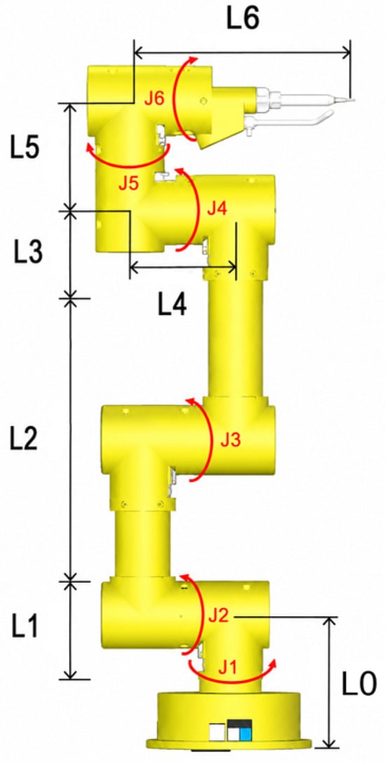
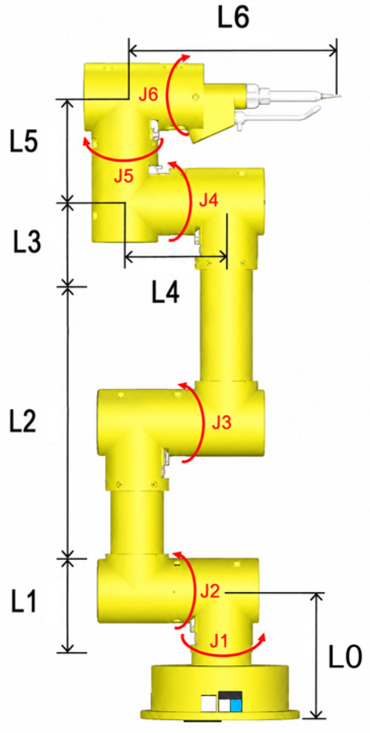
The object of this study is a serial multi-DOF manipulator, whose structural schematic is shown in Figure 1. The goal of manipulator path planning is to generate an executable path that satisfies both kinematic and collision-avoidance constraints under given initial point, goal point, and obstacle constraints, so that the end effector can move safely from the initial position to the target position. Because the end-effector position and the joint variables are related through a nonlinear mapping relationship during manipulator motion, and because collision constraints also exist between the manipulator links and environmental obstacles, it is first necessary to establish a mathematical model and algorithmic framework suitable for the path-planning task studied in this study.

Figure 1. Schematic diagram of the robotic manipulator structure.

To reduce the complexity of directly searching in a high-dimensional joint space, this study adopts an end-effector-based path-planning model. First, the motion state of the manipulator end effector is described in Cartesian space, and the mapping relationship between active joint variables and end-effector position is established through a kinematic model. Then, a basic RRT path-planning model is established in end-effector space to describe random sampling, node extension, and path generation. On this basis, clearance-field constraints and a behavior-cloning trajectory-guidance strategy are introduced to reduce the pronounced stochasticity, excessive path redundancy, and insufficient planning stability of the traditional RRT algorithm.

2.1. End-Effector Kinematic Modeling of the Robotic Manipulator

This study establishes the end-effector kinematic model of the manipulator in Cartesian space. The end-effector position is jointly determined by all joint variables. To describe the correspondence between joint space and end-effector space, the manipulator joint variables and end-effector position variables are first defined, and the kinematic mapping relationship from active joint variables to end-effector position is then established.

Let the complete joint variable vector of the manipulator be

$$q={\left[q_1,q_2,q_3,q_4,q_5,q_6\right]}^T$$

(1)

where $q_1,q_2,q_3,q_4,q_5$ and $q_6$ denote the rotation angles of the manipulator joints. According to the actual structure and control mode of the experimental platform used in this study, the fifth and sixth joints remain fixed during path planning and motion control and are not treated as active planning variables. Therefore:

$$q_5=q_{5,0}, q_6=q_{6,0}$$

(2)

Accordingly, the complete joint state of the manipulator can be represented by selecting the first four joints as active joint variables:

$$q={\left[q_1,q_2,q_3,q_4,q_{5,0},q_{6,0}\right]}^T$$

(3)

The position of the manipulator end effector in Cartesian space is defined as

$$p={\left[x,y,z\right]}^T$$

(4)

where $x,y$ and $z$ denote the three-dimensional coordinates of the manipulator end effector in the IK coordinate system [34]. The forward kinematic model of the manipulator can be expressed as a mapping relationship from the active joint space to the end-effector space [2]:

$$p=f_a\left(q_a\right)$$

(5)

For a serial manipulator, the end-effector pose can be obtained by multiplying the homogeneous transformation matrices between adjacent joints:

$$T_{06}(q)=T_{01}(q_1)·T_{12}(q_2)·T_{23}(q_3)·T_{34}(q_4)·T_{45}(q_{5,0})·T_{56}(q_{6,0})$$

(6)

where $T_{06}(q)$ denotes the homogeneous transformation matrix from the manipulator base coordinate system to the end-effector coordinate system. Since $q_5$ and $q_6$ remain fixed during motion, $T_{45}{q}_{5,0}$ and $T_{56}{q}_{6,0}$ can be regarded as fixed transformation matrices. The end-effector position is obtained from the translational part of $T_{06}(\mathrm{q})$ [2]:

$$p = {[T_{06}(1,4), T_{06}(2,4), T_{06}(3,4)]}^T$$

(7)

The end-effector kinematic model provides the transformation relationship between the manipulator joint configuration and the Cartesian position of the end effector. In this study, trajectory planning is performed in Cartesian space, where the generated collision-free path consists of a sequence of end-effector positions. Therefore, the kinematic model is used together with inverse kinematics to transform the planned Cartesian trajectory into executable joint configurations for the physical manipulator. Only solutions satisfying joint-limit constraints and trajectory continuity requirements are retained for subsequent execution.

2.2. Baseline RRT Path-Planning Model

Based on the end-effector kinematic model of the manipulator [6,7], this study adopts the Rapidly Exploring Random Tree (RRT) algorithm, with the manipulator end effector as the planning object. The baseline RRT is introduced as a reference method to evaluate the effectiveness of the proposed clearance-field-guided sampling mechanism. As a classical sampling-based motion-planning algorithm, RRT has strong exploration capability in high-dimensional spaces without requiring explicit environmental gradients. However, its random sampling strategy may result in redundant nodes, inefficient extensions, and excessive detours, especially in obstacle-constrained regions. Therefore, the baseline RRT provides a necessary comparison benchmark for analyzing the improvements achieved by the proposed method.

Under given search boundary, start point, goal point, and obstacle constraints, the search tree is constructed through random sampling and incremental extension. Let the three-dimensional search space be X and the obstacle region be $X_{obs}$. Then the collision-free space is written as:

$$X_{free} = X \backslash X_{obs}$$

(8)

The path start point and goal point are denoted as $p_{start}$ and $p_{goal}$, respectively, and satisfy

$$p_{start} \in X_{free}, p_{goal} \in X_{free}$$

(9)

The search tree is represented as:

$$T = (V,E)$$

(10)

where V is the set of nodes and E is the set of edges. Initially, the search tree contains only the start point, namely, V = {$p_{start}$} and E = empty set. In each iteration, the algorithm first generates a sampled point according to a goal-bias strategy, then determines the extension node using nearest-neighbor search and finally generates a new node according to a fixed step size. If both the new node and the connecting edge satisfy collision-free constraints, the new node is added to the search tree.

Goal-biased sampling is commonly employed in RRT variants to accelerate tree growth toward the target while retaining stochastic exploration [16,17,18,19]. Accordingly, the goal point is selected as the sampled point with a prescribed probability, whereas uniform random sampling is performed within the search space in the remaining cases.

Distance and proximity information are commonly used in sampling-based motion planning to support collision checking and clearance evaluation [30]. Accordingly, the obstacle boundary is inflated by the prescribed safety margin before each newly generated node and its connecting edge is validated. A node is accepted only if it lies within the search boundary, remains outside the inflated obstacle region, and can be connected to its parent node without collision.

Unlike the conventional RRT implementation, which terminates after obtaining the first feasible solution, the proposed data-generation procedure retains multiple candidate paths. When a newly generated node enters the goal-connection region and can be connected to the goal without collision, a complete candidate path is recovered through parent-node backtracking and added to the candidate-path set. Let the candidate-path set be

$$C=\left\{P_1, P_2,\dots , P_M\right\}$$

(11)

For any discrete path

$$P=\left\{p_0, p_1, \dots , p_n\right\}$$

(12)

Its path length is defined as:

$$L(P) = \sum _i^{n-1}||p_{i+1} - p_i{\left|\right|}_2$$

(13)

Finally, the path with the shortest length is selected from the candidate-path set as the current search result:

$$P_{best} = arg min L(P_j), P_j \in C$$

(14)

The RRT path-generation process used in this study is shown in Algorithm 1 [6,7].

Algorithm 1: Ordinary RRT Expert Trajectory Generation

Input:

$p_{start}$$, p_{goal}$$, X_{free}$$, X_{obs}$$, N_{max}$$, \eta$$, {\epsilon }_{goal}$$, \beta$

Output:

candidate path P or failure

$1: \mathrm{V} \leftarrow \left\{p_{start}\right\}$

$2: \mathrm{E} \leftarrow \varnothing$

$3: \mathrm{Parent} (p_{start}$) ← null

$4: \mathrm{for} \mathrm{k} = 1 \mathrm{to} N_{max}$ do

$5: \mathrm{if} \mathrm{Random} (0,1) < \beta$ then

$6: p_{rand}$$\leftarrow p_{goal}$

7:          else

$8: p_{rand}$$\leftarrow \mathrm{UniformSample} (X_{free}$)

9:          end if

$10: p_{near}$$\leftarrow \mathrm{Nearest} (\mathrm{V}, p_{rand}$)

$11: p_{new}$$\leftarrow \mathrm{Steer} (p_{near}$$, p_{rand}$$, \eta$)

$12: \mathrm{if} p_{new}$$\notin X_{free}$ then

13:                 continue

14:         end if

$15: \mathrm{if} \mathrm{Collision} \mathrm{Free} (p_{near}$$, p_{new}$$, X_{obs}$) = false then

16:                 continue

17:         end if

$18: \mathrm{V} \leftarrow \mathrm{V} \cup \left\{p_{new}\right\}$

$19: \mathrm{E} \leftarrow \mathrm{E} \cup \{(p_{near}$$, p_{new})\}$

$20: \mathrm{Parent} (p_{new}$$) \leftarrow p_{near}$

$21: \mathrm{if} \mathrm{Distance} (p_{new}$$, p_{goal}$$) \le {\epsilon }_{goal}$ then

$22: \mathrm{if} \mathrm{Collision} \mathrm{Free} (p_{new}$$, p_{goal}$$, X_{obs}$) = true then

$23: \mathrm{P} \leftarrow \mathrm{Backtrack} \mathrm{Path} (\mathrm{Parent}, p_{new}$)

$24: \mathrm{P} \leftarrow \mathrm{Append} \mathrm{Goal} (\mathrm{P}, p_{goal}$)

25:                         return P

26:                 end if

27:         end if

28: end for

29: return failure

• where $N_{max}$ is the maximum number of iterations, $\eta$ is the single-step extension length, ${epsilon}_{goal }$ is the goal-connection threshold, and beta is the goal-bias probability. Steer limits the extension distance of the search tree, CollisionFree checks whether the newly generated edge collides with obstacles, and Backtrack Path recovers the complete path from the node near the target according to the parent-node relationship.

Since the first path found by ordinary RRT is usually not optimal, this study repeatedly runs RRT during data generation and stores multiple feasible paths obtained from successful planning, forming the basic expert trajectory set:

$$D_{expert} = \left\{P_1, P_2, \dots , P_M\right\}$$

(15)

where M denotes the number of expert trajectories successfully generated. This dataset is used for subsequent behavior-cloning model training and provides demonstration path samples for the learning-based trajectory-guidance strategy.

2.3. Clearance-Field-Guided Improved RRT Model

Previous studies have shown that weakly guided sampling can generate redundant nodes and inefficient tree expansion in cluttered or narrow regions [15,16,17,18,19,20]. Although baseline RRT can identify feasible paths in three-dimensional space, its stochastic sampling process may produce invalid extensions near obstacles and paths with excessive detours or abrupt local turns. To address these limitations, this study incorporates a clearance-field-guided sampling mechanism into the baseline RRT framework, biasing tree expansion toward locally traversable regions that satisfy the prescribed clearance constraints.

Let the path start point and goal point be $p_{start}$ and $p_{goal}$ [11,12], respectively. The reference direction from the start point to the goal point is defined as:

$$e = {\displaystyle \frac{(p_{goal} - p_{start})}{ ||p_{goal} - p_{start}{||}_2}}$$

(16)

During clearance-field-guided sampling, a slice position is first selected randomly between the start point and the goal point: $t \in \left[0, 1\right]$.

The corresponding slice center is

$$c\left(t\right)=p_{start}+t\left(p_{goal}-p_{start}\right)$$

(17)

At the slice center $c\left(t\right)$, a local slice plane perpendicular to the reference direction e is constructed. Let $u$ and $v$ be two orthogonal unit directions in the slice plane. Then a candidate point inside the slice can be represented as:

$$p_m = c\left(t\right)+ a_m u + b_m v$$

(18)

where m is the candidate-point index, and $a_m$ and $b_m$ are the offsets of the candidate point in the slice plane. To limit the distribution range of candidate points, this study uses an elliptical sampling region in the slice plane to generate candidates:

$$a_m = r_1 \rho cos \theta$$

(19)

$$b_m=r_2 \rho sin \theta$$

(20)

where $r_1$ and $r_2$ are the sampling radii along the two directions in the slice plane, rho is in [0,1], and theta is in [0,2$\pi$]. In this way, candidate points are restricted to a local region near the start-goal reference line, so that sampling preserves the overall goal direction while still leaving space for bypass around obstacles.

For each candidate point $p_m$, the algorithm first determines whether it lies within the search boundary and satisfies collision-free constraints. If the candidate point exceeds the search boundary or falls into the expanded obstacle region, it is regarded as invalid. For a valid candidate point, D ($p_m$) is defined as its distance to the nearest obstacle surface. Let the desired clearance range be [28,30]:

$$d_{min} \le D\left(p_m\right)\le d_{max}$$

(21)

The clearance-band cost function is defined as:

$$\begin{array}{c}{C_{band}(D) = (D - d_{min})}^2 + P_{col}, D < d_{min}\\ C_{band}\left(D\right)= k_b{\left(D - d_{mid}\right)}^2, { d}_{min} \le D \le d_{max}\\ C_{band}\left(D\right)= {\left(D - d_{max}\right)}^2,D > d_{max}\end{array}$$

(22)

where $d_{mid} = (d_{min} + d_{max}) / 2$, $P_{col}$ is the penalty term for excessive proximity or collision, and $k_b$ is the weighting coefficient inside the clearance band. This cost function encourages sampled points to fall within the desired clearance range, avoiding paths that are either too close to collision or unnecessarily far around the obstacle.

To ensure that the clearance constraint mainly acts near obstacles, an obstacle influence factor $\alpha (p)$ is introduced. Let ${lambda}_p$ and ${lambda}_o$ be the projected positions of the candidate point p and the obstacle center $o$ along the reference direction $e$, respectively.

Then

$$\alpha (p)=exp(-{\displaystyle \frac{{({\lambda }_p-{\lambda }_o)}^2}{{2\sigma }^2}})$$

(23)

where $\sigma$ is the obstacle influence-range parameter. When the slice containing the candidate point is close to the obstacle, $\alpha (p)$ is large and the clearance-band constraint has an enhanced effect on sample evaluation. When the candidate point is far from the obstacle, $\alpha (p)$ is small and the sample evaluation is more strongly governed by the reference-line constraint.

Meanwhile, the distance from the candidate point to the start-goal reference line is defined as $D_{line}\left(p\right).$ The distance from the candidate point to the goal point is

$$D_{goal}(p)=||p-p_{goal}{||}_2$$

(24)

Then, the clearance-field evaluation function of the candidate point can be expressed as

$$\Phi (p)=w_l(1-\alpha (p)){D_{line}}^2(p)+w_c \alpha (p)C_{band}(D(p))+w_g {D_{goal}}^2(p)+P_{invalid}\left(p\right)$$

(25)

The weighting parameters $w_l$, $w_c$, and $w_g$ determine the relative importance of reference-line consistency, obstacle clearance, and goal-directed expansion in the clearance-field evaluation function. In this study, these parameters are selected to achieve a balance among path compactness, obstacle-avoidance safety, and search efficiency. A larger $w_l$ increases the preference for samples close to the reference direction, while a larger $w_c$ strengthens the influence of obstacle-clearance constraints and improves safety margins. Increasing $w_g$ promotes faster expansion toward the goal region but may reduce exploration capability if excessive. Therefore, the selected weighting parameters provide balanced trade-offs between trajectory efficiency, safety, and planning stability.

In each field-guided sampling operation, the algorithm generates M candidate points within the current random slice and calculates their clearance-field evaluation values. The candidate point with the minimum cost is finally selected as the field-guided sample:

$$p_{field} = arg min \Phi (p_m), m = 1, 2, \dots , M$$

(26)

During the RRT sampling stage, a sample point is generated in one of three ways [16,17,18,19]:

$$p_{rand} = p_{goal}, with probability {\beta }_g$$

$$p_{rand}=p_{field}, with probability {\beta }_f$$

(27)

$$p_{rand}=p_{uniform}, with probability {\beta }_r$$

where ${\beta }_g$, ${\beta }_f$ and ${\beta }_r$ denote the probabilities of goal-biased sampling, clearance-field-guided sampling, and uniform random sampling, respectively, and satisfy

$${\beta }_g+{\beta }_f+{\beta }_r=1$$

(28)

After the sample point is determined, the subsequent steps are the same as those in basic RRT. Let $p_{near}$ be the node in the current search tree nearest to $p_{rand}$. The new node is then generated by the Steer function:

$$p_{new} = Steer\left(p_{near}, p_{rand}, \eta \right)$$

(29)

If $p_{new}$ lies in collision-free space and the line segment Line ($p_{near}$, $p_{new}$) does not collide with any obstacle, $p_{new}$ is added to the search tree. When $p_{new}$ satisfies the goal-connection condition, the algorithm backtracks according to the parent-node relationship to generate a candidate path.

The main procedure of clearance-field-guided RRT is shown in Algorithm 2.

Algorithm 2: Clearance-field-guided RRT algorithm for expert trajectory generation

$\mathrm{Input}:$

$p_{start}$$, p_{goal}$$, X_{free}$$, X_{obs}$$, \mathrm{D}(\mathrm{p}), d_{min}$$, d_{max},$

$N_{run}$$, N_{max}$$, \eta , {\epsilon }_{goal},$

${\beta }_g$$, {\beta }_f$$, {\beta }_r,$

$\mathrm{M}, r_1$$, r_2$$, \sigma ,$

$w_l$$, w_c$$, w_g$

$\mathrm{Output}:$

$\mathrm{field}\text{-}\mathrm{guided} \mathrm{expert} \mathrm{trajectory} \mathrm{dataset} D_{expert}$

$1: D_{expert}$$\leftarrow$$\varnothing$

$2: \mathrm{e} \leftarrow$$(p_{goal}$$- p_{start}$$)/||p_{goal} - p_{start}{||}_2$

$3: \mathrm{for} \mathrm{run} = 1 \mathrm{to} N_{run}$ do

$4: \mathrm{V} \leftarrow$$\left\{p_{start}\right\}$

$5: \mathrm{E} \leftarrow$$\varnothing$

$6: \mathrm{Parent}(p_{start}$$) \leftarrow$ null

$7: \mathrm{for} \mathrm{k} = 1 \mathrm{to} N_{max}$ do

$8: \mathrm{r} \leftarrow$ Random (0,1)

$9: \mathrm{if} \mathrm{r} < {\beta }_g \mathrm{then}$

$10: p_{rand}\leftarrow p_{goal}$

$11: \mathrm{else} \mathrm{if} \mathrm{r} < {\beta }_g$$+ {\beta }_f$ then

$12: \mathrm{t} \leftarrow \mathrm{Random} (0,1)$

$13: \mathrm{c} \leftarrow p_{start}$$+ \mathrm{t}(p_{goal}$$- p_{start})$

$14: \Pi \leftarrow \mathrm{Plane} (\mathrm{c}, \mathrm{e})$

$15: X_{candidate}\leftarrow \varnothing$

$16: \mathrm{for} \mathrm{m} = 1 \mathrm{to} \mathrm{M} \mathrm{do}$

$17: p_m \mathrm{Sample} \mathrm{Ellipse} (\Pi$$, r_1$$, r_2)$

$18: \mathrm{if} \mathrm{not} \mathrm{Inside} \mathrm{Bounds} (p_m)$ then

19:                                               continue

20:                                       end if

$21: \mathrm{if} p_m$$\notin X_{free}$ then

22:                                               continue

23:                                       end if

$24: D_m\leftarrow \mathrm{Distance} \mathrm{to} \mathrm{Obstacle} \mathrm{Surface} (p_m$$, X_{obs})$

$25: {\alpha }_m\leftarrow \mathrm{Obstacle} \mathrm{Influence} (p_m$$, X_{obs}$$, \mathrm{e}, \sigma )$

$26: D_{line}\leftarrow \mathrm{Distancetoo} \mathrm{Reference} \mathrm{Line}(p_m$$, p_{start}$$, p_{goal})$

$27: D_{goal}\leftarrow \mathrm{Distance} (p_m$$, p_{goal})$

$28: \Phi$$(p_m$$) \leftarrow$$w_l$$(1 - {\alpha }_m$$){ D}_{line}^2$$+ w_c$${\alpha }_m$$C_{band}$$(D_m$$) + w_g$$D_{goal}^2$

$29: X_{candidate}$$\leftarrow$$X_{candidate}$$\cup$$\{p_m\}$

30:                                 end for

$31: p_{rand}$$\leftarrow$$\arg \min \Phi$$(p_m$$), p_m$$\in$$X_{candidate}$

$32: \mathrm{else}$

$33: p_{rand}$$\leftarrow$$\mathrm{Uniform} \mathrm{Sample} (X_{free})$

34:                          end if

$35: p_{near}$$\leftarrow$$\mathrm{Nearest} (\mathrm{V}, p_{rand})$

$36: p_{new}$$\leftarrow$$\mathrm{Steer} (p_{near}$$, p_{rand}$$, \eta )$

$37: \mathrm{if} \mathrm{not} \mathrm{Inside} \mathrm{Bounds} (p_{new})$ then

38:                                   continue

39:                          end if

$40: \mathrm{if} \mathrm{not} \mathrm{Collision} \mathrm{Free} (p_{near}$$, p_{new}$$, X_{obs})$ then

41:                                   continue

42:                          end if

$43: \mathrm{V} \leftarrow$$\mathrm{V} \cup$$\{p_{new}\}$

$44: \mathrm{E} \leftarrow$$\mathrm{E} \cup$$\{(p_{near}$$, p_{new})\}$

$45: \mathrm{Parent}(p_{new}$$) \leftarrow$$p_{near}$

$46: \mathrm{if} \mathrm{Distance} (p_{new}$$, p_{goal}$$) \le$${\epsilon }_{goal}$ then

$47: \mathrm{if} \mathrm{Collision} \mathrm{Free} (p_{new}$$, p_{goal}$$, X_{obs})$ then

$48: \mathrm{P} \leftarrow$$\mathrm{Backtrack} \mathrm{Path} (\mathrm{Parent}, p_{new})$

$49: \mathrm{P} \leftarrow$$\mathrm{Append} \mathrm{Goal} (\mathrm{P}, p_{goal})$

$50: D_{expert}\leftarrow D_{expert}$$\cup$ {P}

51:                                           break

52:                                   end if

53:                           end if

54:                   end for

55: end for

$56:\mathrm{return} D_{expert}$

After candidate paths are generated, this approach further filters them according to path length, smoothness, clearance, and maximum turning angle. The total path cost can be written as [31,32]:

$$J_{path}\left(P\right)= w_1 L\left(P\right)+ w_2 S\left(P\right)+ w_3 C_{clear}\left(P\right)+ w_4 C_{turn}\left(P\right)$$

(30)

where $L(P)$ is the path length, S(P) is the path-smoothness term, $C_{clear}$(P) is the minimum-clearance penalty, and $C_{turn}(P)$ is the maximum-turning-angle penalty. Accordingly, the path smoothness index is defined as:

$$S(P)={\displaystyle \sum _{i=1}^{n-1}}\left(1-\mathrm{c}\mathrm{o}\mathrm{s}{\theta }_i\right)$$

(31)

Finally, the path with the minimum total cost that satisfies collision, clearance, and maximum-turning-angle constraints is selected from the candidate-path set as the expert trajectory.

2.4. Behavior-Cloning-Based Trajectory Guidance Strategy

The preceding RRT and Field-guided RRT methods can generate many reference path samples that satisfy collision-avoidance constraints. However, these path-generation processes usually require repeated searching or candidate-point screening, and their computational efficiency and path stability are affected by sampling randomness. To reduce reliance on repeated random search, this study further adopts behavior cloning, converting the reference path samples generated by the planner into supervised-learning data and learning the mapping relationship from the current state to the next-step motion direction.

Let the set of reference paths generated and filtered by the path planner be

$$D=\{P_1, P_2, \dots , P_N\}$$

(32)

where the j-th reference path is

$$P_j=\left\{p_0, p_1, \dots , p_n\right\}$$

(33)

For adjacent points $p_i$ and $p_{i+1}$ on a path, a state-action sample is constructed: $\left(s_i, a_i\right),$ where $s_i$ is the current state vector and $a_i$ is the reference action vector. In this study, the behavior-cloning model has an input dimension of 14 and an output dimension of 3.

According to the data structure in the implemented program, the state vector is defined as:

$$s_i ={\left[\begin{array}{c}{s}_{px}, s_{py}, s_{pz}, s_{goal,dx}, s_{goal,dy}, s_{goal,dz}, s_{obs,dx},\\ s_{obs,dy}, s_{obs,dz}, s_{obs,sx}, s_{obs,sy}, s_{obs,sz}, s_{dist,goal}, s_{dist,obs}\end{array}\right]}^T, s_i \in R^{14}$$

(34)

where $s_{px}$, $s_{py}$, and $s_{pz}$ denote the normalized current end-effector position.

$s_{goal,dx}$, $s_{goal,dy}$, and $s_{goal,dz}$ denote the normalized relative vector from the current point to the goal point.

$s_{obs,dx}$, $s_{obs,dy}$, and $s_{obs,dz}$ denote the normalized relative vector from the current point to the obstacle center.

$s_{obs,sx}$, $s_{obs,sy}$, and $s_{obs,sz}$ denote the normalized obstacle dimensions.

$s_{dist,goal}$ and $s_{dist,obs}$ denote the normalized distance from the current point to the goal point and the normalized distance from the current point to the obstacle, respectively.

The reference action is obtained from the unit direction vector between adjacent path points:

$$a_i = (p_{i+1} - p_i) / ||p_{i+1} - p_i{||}_{2 }$$

(35)

where $a_i \in R^3$ and it satisfies: $\left|\right|a_i{\left|\right|}_2 = 1$.

Therefore, the behavior-cloning model learns the next-step motion direction provided by the reference path under the current state, rather than the absolute coordinates of the next path point:

$${\pi }_{\theta } : R^{14} \to R^3$$

(36)

where theta denotes the network parameters. Given state $s_i$, the network outputs the predicted action:

$$a_{hat,i} = {\pi }_{\theta }\left(s_i\right)$$

(37)

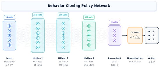
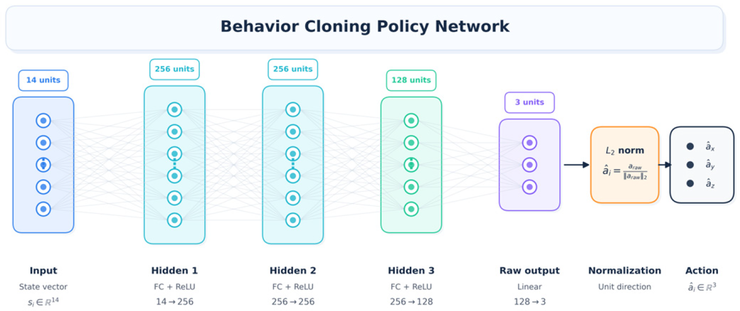
According to the implemented parameter settings, the behavior cloning policy network contains three hidden layers with dimensions of 256, 256, and 128, respectively, and ReLU is used as the activation function. The network structure is shown in Figure 2, and its mapping process can be expressed as follows:

$$h_1 = ReLU(W_1 s_i + b_1)$$

$$h_3=ReLU(W_3 h_2+b_3)$$

(38)

$$a_{raw}=W_{4h,3}+b_4$$

Figure 2. Architecture of the multilayer perceptron policy network for behavior cloning.

Because the action represents a three-dimensional motion direction, the network output must be normalized to unit length:

$$a_{hat,i} = a_{raw} / ||a_{raw}{||}_2$$

(39)

Thereby satisfying

$$||a_{hat,i}{||}_2=1$$

(40)

The objective of behavior-cloning training is to make the predicted action $a_{hat,i}$ close to the reference action $a_i$. Since the actions are unit direction vectors, this study constructs the loss function using both mean squared error and cosine directional error:

$$L_{BC}\left(i\right)= w_{mse} {||a_{hat,i} - a_i{||}_2}^2 + w_{cos}\left(1 - a_{hat,i} · a_i\right)$$

(41)

where $w_{mse}$ and $w_{cos}$ are the weights of the mean-squared-error term and the cosine-direction-error term, respectively. In the implemented planning program, $w_{mse} = 0.5$, and $w_{cos} = 0.5$.

Therefore, the overall optimization objective is

$${\theta }^{*}=\mathrm{a}\mathrm{r}\mathrm{g}{\mathrm{m}\mathrm{i}\mathrm{n}}_{\theta }\sum _i\left[0.5{‖{\pi }_{\theta }(s_i)-a_i‖}_2^2+0.5\left(1-{\pi }_{\theta }(s_i)·a_i\right)\right]$$

(42)

To prevent adjacent points from the same path from appearing simultaneously in the training and verification sets, this study divides samples according to ${run}_{id}$. By default, samples satisfying

$${run}_{id} mod 10=9$$

(43)

are used as the verification set, and the remaining samples are used as the training set. This approach splits the data at the path level and reduces data leakage caused by adjacent path points.

After training is completed, given the current state $s_t$, the behavior-cloning model outputs the next-step unit motion direction:

$$a_t = {\pi }_{\theta }\left(s_t\right)$$

(44)

After combining this value with the specified step size η, the next end-effector position can be obtained, as

$$p_{t+1}=p_t+{\eta a}_t$$

(45)

The newly generated position must then be further verified against boundary constraints, collision constraints, and kinematic executability.

3. RRT Offline Training, Simulation-Assisted Validation and Obstacle-Avoidance Trajectory Verification

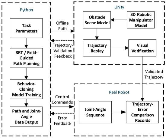
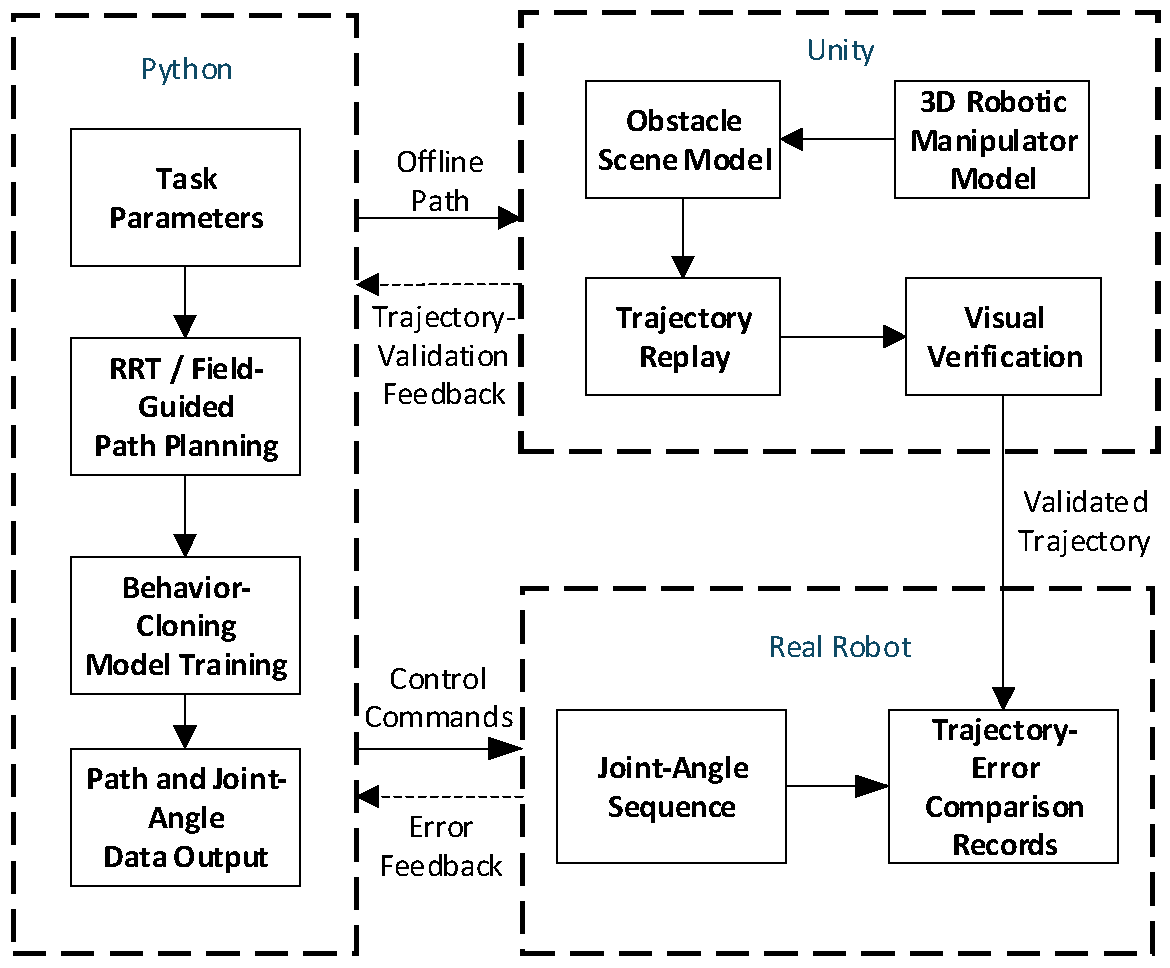
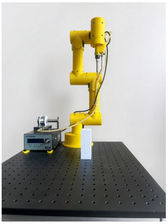
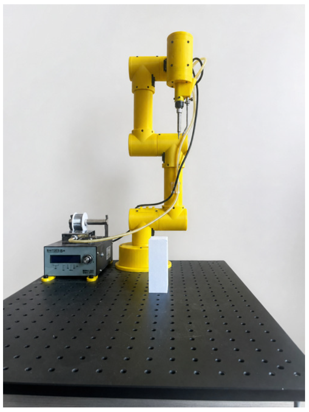
To verify the effectiveness of the proposed RRT offline training method in manipulator collision-free path planning and its executability in a three-dimensional manipulator scene, this study constructs a joint simulation–verification platform based on Python and Unity. As shown in Figure 3, the platform uses the Python side as the core for path planning, data generation, and result analysis, while the Unity side serves as the environment for three-dimensional manipulator modeling, trajectory replay, and visual verification. A hardware manipulator experimental platform, as show in Figure 4, is also used for further verification of the planned trajectory.

Figure 3. Structural block diagram of the Python–Unity joint simulation–verification platform.

Figure 4. Physical manipulator experimental platform.

The platform mainly consists of a Python offline-planning module, a Unity three-dimensional simulation–verification module, and a hardware manipulator experimental-verification module. The Python side is responsible for task-parameter setting, RRT and Field-guided RRT path planning, behavior-cloning model training, path-point calculation, and joint-angle data export. The Unity side builds the three-dimensional manipulator model and obstacle-scene model, reads the offline path files output by Python, and replays and visually verifies the end-effector trajectory, thereby assessing the obstacle-avoidance effect and spatial reachability of the planned path in a three-dimensional simulation environment.

In the data-interaction process, the offline path and joint-angle data generated by Python are first input into the Unity environment for simulation verification. If the trajectory can complete obstacle-avoidance replay in Unity and satisfies the end-effector goal-reaching and path-safety requirements, the corresponding joint-angle sequence is then used as the control input for the hardware manipulator. During hardware execution, the actual joint angles, end-effector trajectory, and error data are recorded and fed back to the Python side for comparative analysis. Therefore, Python and the hardware manipulator form a verification relationship of “control-command output–hardware execution–error-feedback analysis”, while Unity and the hardware manipulator are mainly compared through trajectory files exported by Python and experimental records.

It should be noted that the platform constructed in this study is not a real-time closed-loop control platform, but an offline joint simulation and experiment-assisted platform intended for validating path-planning algorithms. With this platform, trajectories generated by different RRT path-planning methods can be replayed, compared, and evaluated in a unified way. Planning effectiveness can then be analyzed using metrics such as path length, minimum clearance, trajectory smoothness, end-effector positioning error, and joint-motion continuity, providing a basis for subsequent collision-avoidance trajectory validation and hardware manipulator experiments.

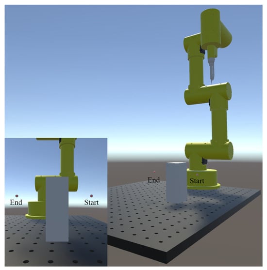
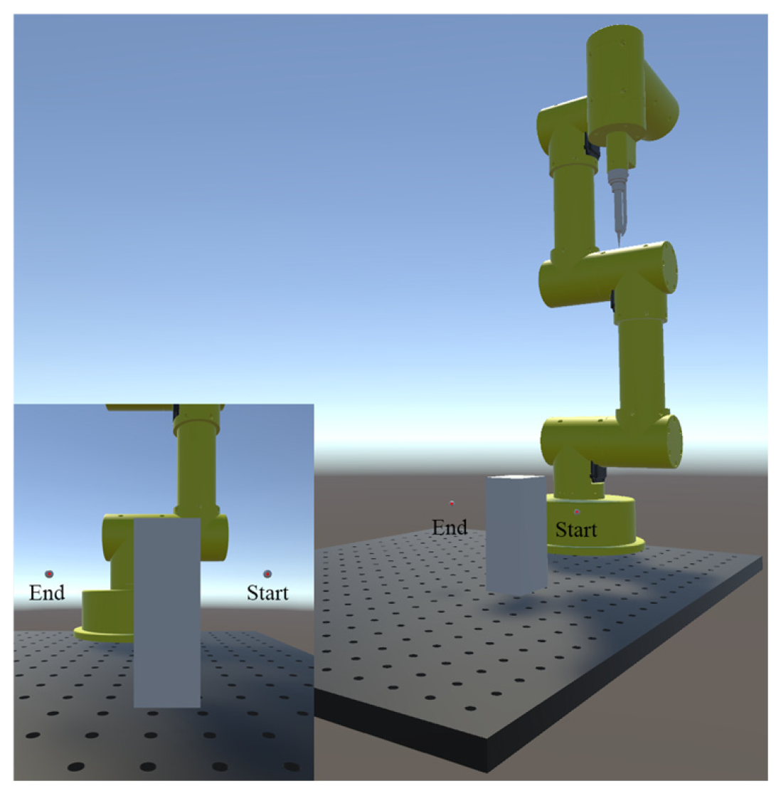
Offline path generation and behavior-cloning training were implemented in Python 3.10 on a Windows platform, while Unity 6000.3.8f1 was used for three-dimensional trajectory visualization and replay. All computations were performed on a workstation equipped with a 12th Gen Intel Core i7-12700H processor and an NVIDIA GeForce RTX 3070 Ti Laptop GPU. To ensure a consistent comparison among the planning methods, the same Cartesian planning environment was used throughout. The start and goal positions were set to ${[-0.100, 0.080, 0.225]}^T$ m and ${[0.030, 0.080, 0.225]}^T$ m, respectively. The corresponding start–goal configuration and obstacle arrangement in the Unity environment are shown in Figure 5. The obstacle was modeled as an axis-aligned cuboid with center ${\left[-0.040, 0.058, 0.223\right]}^T \mathrm{m}$ and dimensions ${[0.035, 0.100, 0.050]}^T$ m. The search domain was defined by $x\in [-0.185, 0.115] \mathrm{m}$, $\mathrm{y}\in [0.030, 0.530] \mathrm{m}$, and $z\in [0.125, 0.325] \mathrm{m}$. During collision checking, the obstacle boundary was enlarged according to the prescribed safety margin. Standard RRT, Clearance-filtered RRT, and Field-guided RRT were evaluated under the same scene configuration and planning constraints.

Figure 5. Schematic of goal-point and obstacle arrangement in Unity.

3.1. RRT Offline Data Generation and Behavior-Cloning Training

Based on the Python–Unity joint simulation–verification platform, this study conducts experiments on RRT offline path-data generation and behavior-cloning model training in the Python environment.

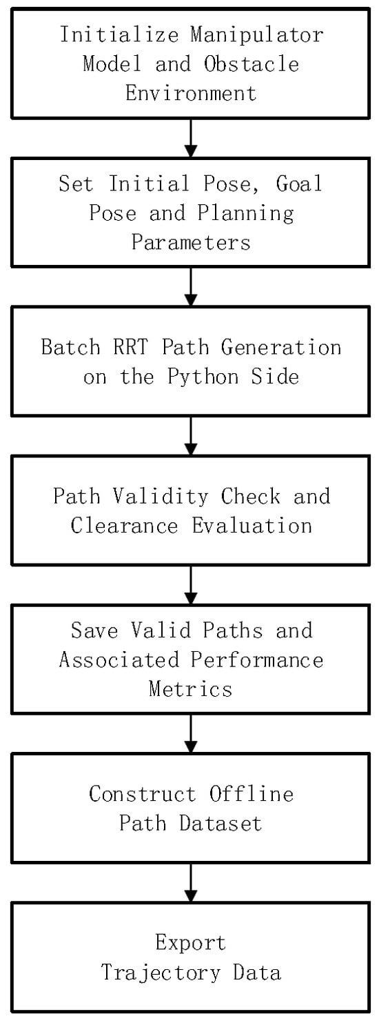
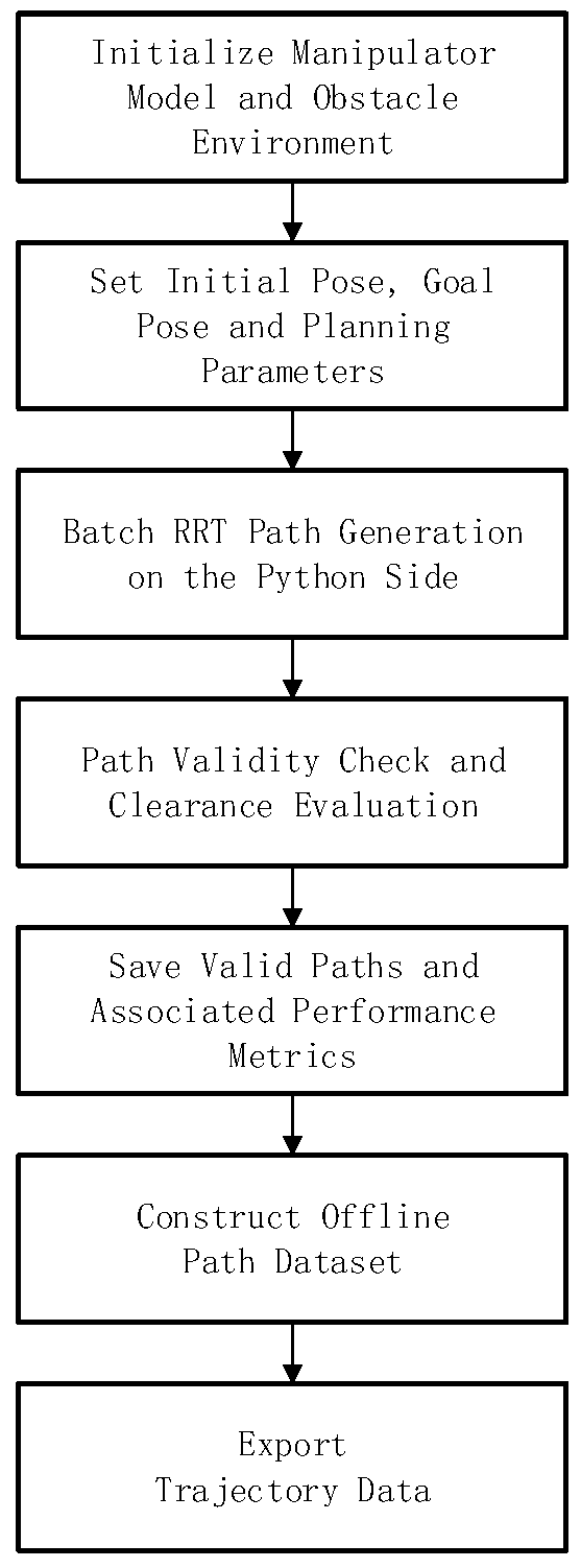
The generation process for the RRT offline expert trajectory dataset is shown in Figure 6. The planning environment is first established, based on the manipulator structural parameters and obstacle configuration. Subsequently, the start point, goal point, search boundary, clearance threshold, and path-planning parameters are specified. In the offline expert trajectory generation process, three types of path data are constructed. The first is Standard RRT, namely, the basic random-sampling path. This method performs goal-biased sampling and random-tree expansion in the given search space to obtain basic feasible collision-free paths. The second is Clearance-filtered RRT, namely, a path constrained by clearance. This method further introduces collision detection, minimum clearance, and path-validity screening on the basis of RRT-generated paths to obtain expert trajectories that satisfy collision-avoidance safety-distance requirements. The third is Field-guided RRT, namely, the clearance-field-guided path. This method introduces evaluation terms such as obstacle distance, reference-line offset, and goal distance during RRT sampling, causing sampled points more preferentially to be distributed in collision-free passage regions near obstacles, and thereby improving the directionality and effectiveness of path search.

Figure 6. Flowchart for generating the RRT offline expert trajectory dataset.

For each successfully generated end-effector path, the implemented program further performs collision-state checking, path-length calculation, clearance evaluation, and trajectory-continuity assessment. Paths that satisfy the constraints are saved as a valid expert trajectory dataset and used as the data source for subsequent behavior-cloning model training.

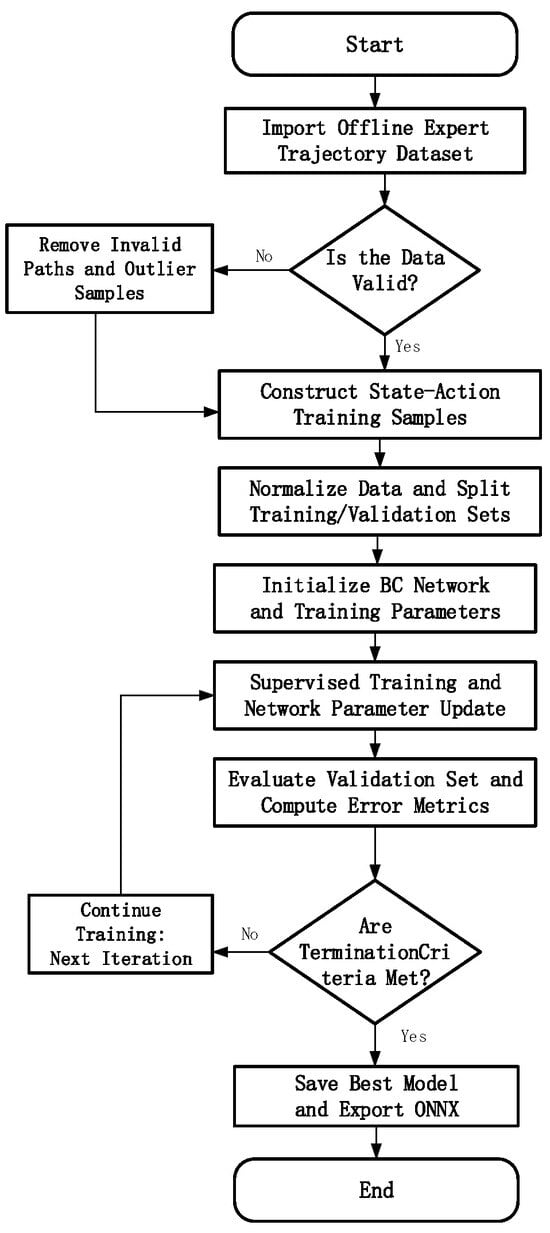
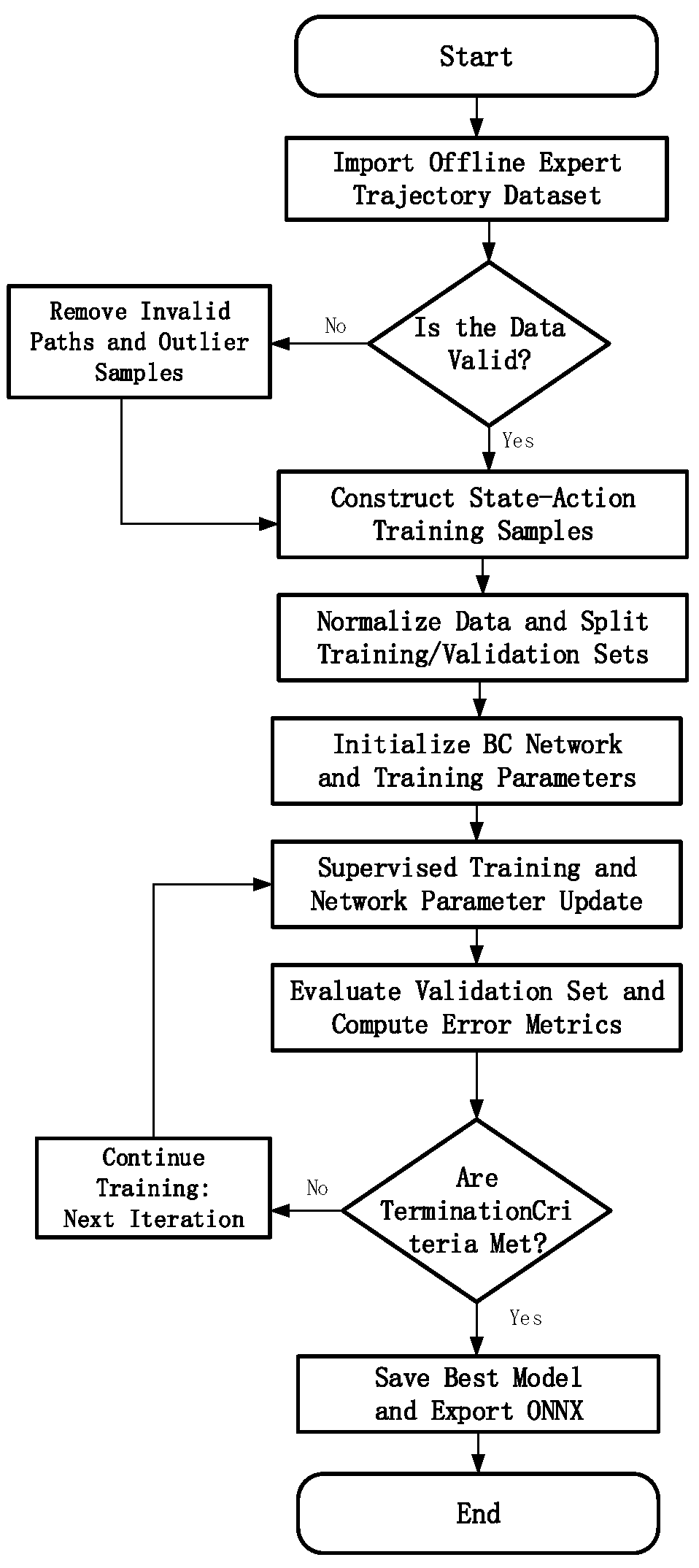
After the offline expert trajectory dataset is obtained, behavior-cloning model training is carried out according to the process shown in Figure 7. Each expert trajectory is converted into multiple state-action samples. The state vector consists of the current end-effector position and its spatial relationships with the goal point and obstacle, while the action vector is defined as the unit direction vector from the current path point to the next path point. After data cleaning and normalization, the samples are divided into training and verification sets. To ensure comparability among training results from different data sources, the three expert-trajectory datasets are trained using the same network structure and training parameters.

Figure 7. Flowchart of behavior-cloning model training.

The cloning model takes a fourteen-dimensional state feature vector as input and outputs a three-dimensional unit-direction action. The expert dataset $D_{expert}$ used for behavior-cloning training contains approximately 100,000 expert state-action samples generated from the offline RRT-based trajectories. The model is trained using the AdamW optimizer, with a learning rate of $3\times {10}^{-4}$, a batch size of 4096, and 20 training epochs. During training, the model fits the mapping relationship from the current state to the expert local motion direction through supervised learning, and the model corresponding to the lowest verification-set loss is saved as the final model [35]. The behavior-cloning training results under different expert trajectory data are shown in Table 1.

Table 1. Training performance of BC models trained with different expert trajectory datasets.

Method	Epoch	Training Loss	Validation Loss	Training Angle Error ($\mathbf{°}$)	Validation Angle Error ($\mathbf{°}$)
Standard RRT + BC	3	0.1792	0.1818	32.31	32.60
Clearance-filtered RRT + BC	17	0.1700	0.1914	31.11	33.57
Field-guided RRT + BC	23	0.1858	0.1902	33.61	33.85

In Table 1, the best result for epoch is considered the epoch at which the verification loss reaches its minimum during training and the model is saved, rather than the manually specified total number of training epochs. The table indicates that the optimal saved epochs differ across expert trajectory datasets, indicating that the expert trajectories generated by the three RRT methods are not completely consistent in sample distribution or local motion characteristics.

Standard RRT + BC reaches the lowest verification loss at epoch 3, indicating that the local motion patterns in expert trajectories generated by Standard RRT are relatively easy to fit. Clearance-filtered RRT + BC and Field-guided RRT + BC achieve their best verification results at epochs 17 and 23, respectively, suggesting that expert trajectories after clearance filtering or clearance-field guidance contain more complex local obstacle-avoidance features and require more training epochs to reach better verification performance.

From the loss-function and angular-error results, all three behavior-cloning models can learn local motion-direction patterns from expert trajectories. Standard RRT + BC has the lowest verification loss and a comparatively small verification angle error, while Clearance-filtered RRT + BC and Field-guided RRT + BC have slightly higher verification angle errors. This suggests that, under the same network structure, expert trajectories with enhanced collision-avoidance constraints place higher demands on the fitting ability of the model. Therefore, differences in the best epoch mainly reflect differences in model convergence under different expert trajectory data. The final performance of each method still needs to be evaluated comprehensively together with subsequent trajectory-replay results, trajectory smoothness, collision-avoidance safety, and end-effector arrival accuracy.

To verify performance differences among path-planning methods in the manipulator collision-avoidance task, this study compares six methods: Standard RRT, Standard RRT + BC, Clearance RRT, Clearance RRT + BC, Field-guided RRT, and Field-guided RRT + BC. BC denotes behavior cloning, a supervised-learning-based method used to predict the local motion direction from expert trajectory data. The evaluation metrics include path length, minimum clearance, smoothness index, maximum turning angle, and trajectory generation time. Path length represents the total Euclidean length of the generated end-effector trajectory. Minimum clearance denotes the minimum distance between the trajectory and the obstacle surface, and is used to evaluate obstacle-avoidance safety. The smoothness index characterizes the accumulated variation in direction between consecutive trajectory segments, with a smaller value indicating better trajectory continuity. Maximum turning angle represents the largest local directional change along the trajectory. Trajectory generation time refers to the computational time required by the RRT-based planner to search for and generate a valid collision-free trajectory. For the BC-based methods, the trained policy directly predicts the local motion direction through network inference without performing the iterative RRT tree-search process; therefore, the RRT-based trajectory generation time is not applicable and is denoted by “–” in Table 2. The results are shown in Table 2.

Table 2. Performance comparison of different RRT-based trajectory planning methods.

Method	Path Length (mm)	Minimum Clearance (mm)	Smoothness Index	Maximum Turning Angle ($\mathbf{°}$)	Time (s)
Standard RRT	349.27	24.45	20.29	99.40	2.9
Standard RRT + BC	266.72	24.53	0.364	14.81	-
Clearance RRT	252.44	6.88	14.591	98.99	83.2
Clearance RRT + BC	203.52	3.9	0.372	18.98	-
Field-guided RRT	240.84	7.87	12.48	93.32	2.2
Field-guided RRT + BC	188.63	1.37	3.345	89.94	-

As shown in Table 2, Standard RRT generated the longest path (349.27 mm) and exhibited pronounced local turning, whereas Clearance RRT reduced the path length to 252.44 mm but required 83.2 s of computation. Field-guided RRT achieved a shorter path of 240.84 mm and reduced the planning time to 2.2 s while maintaining a minimum clearance of 7.87 mm. These results indicate that clearance-field guidance improves the directionality of tree expansion and provides a better balance between path compactness, planning efficiency, and obstacle clearance.

The introduction of behavior cloning generally reduced path length and improved trajectory continuity. Standard RRT + BC and Clearance RRT + BC achieved substantially lower smoothness indices and maximum turning angles than their corresponding baseline methods. Field-guided RRT + BC produced the shortest path (188.63 mm); however, it approached the obstacle more closely under the prescribed clearance threshold and retained a relatively large maximum turning angle. Therefore, among the non-learning planners, Field-guided RRT demonstrated the best overall performance, whereas behavior cloning was more effective as an auxiliary strategy for offline trajectory refinement.

3.2. Simulation-Assisted Validation Results

To further verify the feasibility of the offline-generated trajectories in a three-dimensional manipulator environment, this study imports the trajectory data generated on the Python side into the Unity platform for simulation-assisted verification. In Unity, a manipulator model, obstacle position, and goal pose consistent with the Python planning environment are constructed to reproduce the collision-avoidance motion of the manipulator from the initial state to the target state.

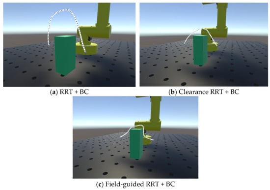
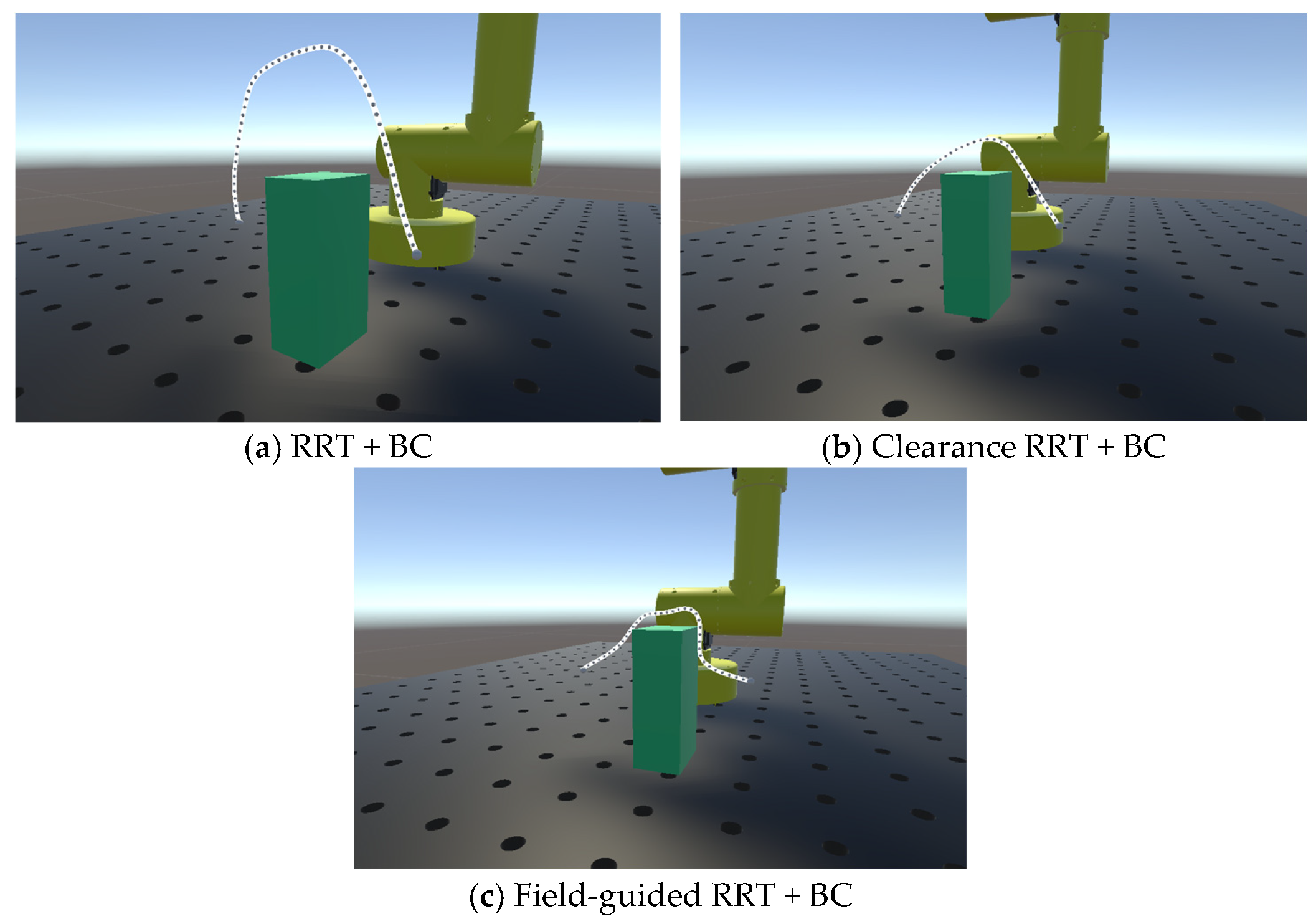
Figure 8 confirms that all three BC-based trajectories can be reproduced in Unity without collision and can successfully reach the goal region. Their geometric characteristics, however, differ: Standard RRT + BC produces a relatively conservative detour, Clearance RRT + BC yields a smoother and more compact trajectory, and Field-guided RRT + BC follows the most direct route while operating closer to the obstacle boundary, within the prescribed clearance criterion. Together with Table 2, these results show that behavior cloning generally improves path compactness or continuity, although the improvement depends on the quality and distribution of the corresponding expert trajectories. In particular, Field-guided RRT + BC achieves the shortest path, whereas its relatively large maximum turning angle indicates that path-length reduction does not necessarily lead to uniformly improved local smoothness.

Figure 8. Reproduction results of obstacle-avoidance trajectories for different methods in Unity.

Considering all methods evaluated, Field-guided RRT provides the most favorable overall balance among path length, planning time, and obstacle clearance. It reduces both path length and computation time relative to Standard RRT and avoids the substantial computational overhead of Clearance RRT, while maintaining a minimum clearance of 7.87 mm. Therefore, the Field-guided RRT trajectory was selected for physical-manipulator validation. The start pose, goal pose, and obstacle configuration were kept consistent with the simulation scene, and the Cartesian path generated in Python was converted into an executable joint-angle sequence through inverse kinematics before being transferred to the physical manipulator [2].

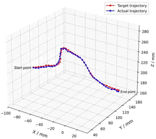
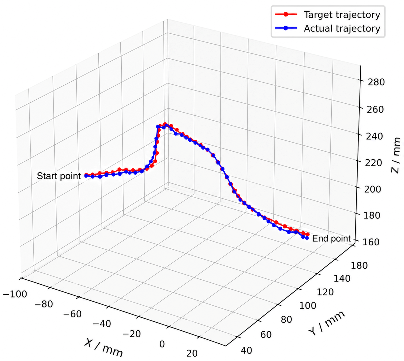
Figure 9 presents the comparison between simulated trajectory points and trajectory points executed by the hardware manipulator. The results indicate that the manipulator can move from the initial pose to the goal pose according to the planned trajectory and complete obstacle avoidance when approaching the obstacle region. Throughout the execution process, the manipulator end effector does not collide with the obstacle, and the overall trend of the actual trajectory is consistent with the Unity simulation reproduction. This suggests that the path generated by Field-guided RRT can not only be visually reproduced in the simulation environment, but also has a measurable degree of executability on a hardware manipulator.

Figure 9. Comparison between the planned and measured end-effector trajectories.

As shown in Table 3, after the hardware manipulator executes the Field-guided RRT trajectory, the end-effector positioning error is 3.8 mm, the average positioning error is 3.7 mm, the maximum joint-angle error is 0.995°, and the average joint-angle error is 0.432°. These deviations indicate that the planned trajectory can be successfully mapped into the joint space of the hardware manipulator after inverse-kinematics conversion. The positioning errors observed during hardware execution mainly arise from servo positioning accuracy, mechanical clearance, joint-control resolution, and assembly deviations between the simulation model and the real mechanism. It should be noted that the purpose of the hardware experiment in this study is not to evaluate the absolute positioning accuracy of the manipulator control system, but to verify the transferability and executability of the generated collision-free trajectory on a physical robotic platform. The experimental manipulator is a prototype platform with limited servo accuracy and without additional high-precision calibration or online compensation mechanisms. Therefore, the measured positioning deviation mainly reflects the execution uncertainty of the hardware platform rather than the planning error of the proposed Field-guided RRT method.

Table 3. Error statistics for hardware manipulator trajectory execution.

End-Effector Positioning Error (mm)	Average Positioning Error (mm)	Maximum Joint-Angle Error ($\mathbf{°}$)	Average Joint Error ($\mathbf{°}$)
3.8	3.7	0.995	0.432

By combining the Unity simulation reproduction results with the experimental results from the hardware manipulator, it can be observed that the collision-free path generated by Field-guided RRT can be effectively verified on both the simulation platform and the hardware platform. The method can not only generate an end-effector path satisfying collision-avoidance constraints but also convert that path into an executable joint-angle sequence for the hardware manipulator through inverse kinematics, validating the practical feasibility of the proposed path-planning method in manipulator collision-avoidance tasks.

4. Conclusions

This paper addresses end-effector obstacle-avoidance trajectory planning for industrial robotic manipulators by combining clearance-field-guided RRT planning, behavior-cloning-based trajectory refinement, Unity-based simulation, and physical-robot validation. To reduce the blind expansion, path redundancy, and unstable planning performance of conventional RRT, a Field-guided RRT method was developed. The proposed planner evaluates candidate samples using obstacle clearance, reference-line deviation, and goal distance, thereby directing tree expansion toward locally traversable regions while preserving global exploration capability.

Comparative results demonstrate that Field-guided RRT achieved the best overall performance among the non-learning planners. Relative to Standard RRT, it reduced the path length from 349.27 mm to 240.84 mm and the planning time from 2.9 s to 2.2 s, while maintaining a minimum obstacle clearance of 7.87 mm. It also resulted in substantially less computational cost relative to Clearance RRT, whose planning time reached 83.2 s. These results confirm that clearance-field guidance improves sampling efficiency and path compactness without sacrificing the prescribed obstacle-clearance requirement.

Behavior cloning was further investigated as an offline trajectory-refinement strategy. Standard RRT + BC and Clearance RRT + BC showed marked improvements in smoothness and maximum turning angle, whereas Field-guided RRT + BC produced the shortest path, 188.63 mm. However, the minimum clearance for Field-guided RRT + BC decreased to 1.37 mm and its maximum turning angle remained relatively large. Thus, behavior cloning was effective for learning local motion trends and refining selected trajectory characteristics, but it did not consistently improve all safety and smoothness metrics. Under the evaluated conditions, Field-guided RRT therefore provided the most balanced performance, while behavior cloning was better suited as an auxiliary offline refinement method.

The planned trajectories were subsequently validated through a Python–Unity workflow and physical-manipulator experiments. Unity-based replay confirmed that the generated end-effector paths could avoid the obstacle and reach the target region in the three-dimensional scene. The selected Field-guided RRT trajectory was then converted into a joint-angle sequence through inverse kinematics and executed on the physical manipulator. The measured end-effector positioning error was 3.8 mm, the average positioning error was 3.7 mm, the maximum joint-angle error was $0.995°$, and the average joint-angle error was $0.432°$. These results verify the spatial feasibility and practical executability of the proposed trajectory-planning method.

Overall, the proposed Field-guided RRT outperformed the baseline planners in the evaluated obstacle-avoidance task by providing a favorable balance among path length, planning time, and obstacle clearance. The integrated simulation and physical validation further demonstrated that the planned Cartesian paths can be reliably transformed into executable manipulator motions. The current study is limited to a static obstacle, fixed start–goal configurations, and a representative experimental scene. Future work will extend the method to multi-obstacle and dynamic environments, online replanning, trajectory time parameterization, joint-dynamic constraints, and execution-error compensation.

References

- LaValle, S.M. Planning Algorithms; Cambridge University Press: Cambridge, UK, 2006. [Google Scholar]
- Siciliano, B.; Khatib, O. (Eds.) Springer Handbook of Robotics; Springer: Berlin/Heidelberg, Germany, 2008. [Google Scholar]
- Orthey, A.; Chamzas, C.; Kavraki, L.E. Sampling-Based Motion Planning: A Comparative Review. Annu. Rev. Control Robot. Auton. Syst. 2024, 7, 285–310. [Google Scholar] [CrossRef] [Scilit]
- Luo, S.; Zhang, M.; Zhuang, Y.; Ma, C.; Li, Q. A Survey of Path Planning of Industrial Robots Based on Rapidly Exploring Random Trees. Front. Neurorobot. 2023, 17, 1268447. [Google Scholar] [CrossRef] [Scilit] [PubMed]
- Xu, T. Recent Advances in Rapidly-Exploring Random Tree: A Review. Heliyon 2024, 10, e32451. [Google Scholar] [CrossRef] [Scilit] [PubMed]
- LaValle, S.M.; Kuffner, J.J. Randomized Kinodynamic Planning. In Proceedings of the 1999 IEEE International Conference on Robotics and Automation, Detroit, MI, USA, 10–15 May 1999; IEEE: New York, NY, USA, 1999; pp. 473–479. [Google Scholar]
- LaValle, S.M.; Kuffner, J.J. Rapidly-Exploring Random Trees: Progress and Prospects. In Algorithmic and Computational Robotics: New Directions; Donald, B.R., Lynch, K.M., Rus, D., Eds.; A K Peters: Wellesley, MA, USA, 2001; pp. 293–308. [Google Scholar]
- Kuffner, J.J.; LaValle, S.M. RRT-Connect: An Efficient Approach to Single-Query Path Planning. In Proceedings of the 2000 IEEE International Conference on Robotics and Automation, San Francisco, CA, USA, 24–28 April 2000; IEEE: New York, NY, USA, 2000; pp. 995–1001. [Google Scholar]
- Karaman, S.; Frazzoli, E. Incremental Sampling-Based Algorithms for Optimal Motion Planning. arXiv 2010, arXiv:1005.0416. [Google Scholar]
- Karaman, S.; Frazzoli, E. Sampling-Based Algorithms for Optimal Motion Planning. Int. J. Robot. Res. 2011, 30, 846–894. [Google Scholar] [CrossRef] [Scilit]
- Gammell, J.D.; Srinivasa, S.S.; Barfoot, T.D. Informed RRT*: Optimal Sampling-Based Path Planning Focused via Direct Sampling of an Admissible Ellipsoidal Heuristic. In Proceedings of the 2014 IEEE/RSJ International Conference on Intelligent Robots and Systems, Chicago, IL, USA, 14–18 September 2014; IEEE: New York, NY, USA, 2014; pp. 2997–3004. [Google Scholar]
- Gammell, J.D.; Barfoot, T.D.; Srinivasa, S.S. Informed Sampling for Asymptotically Optimal Path Planning. IEEE Trans. Robot. 2018, 34, 966–984. [Google Scholar] [CrossRef] [Scilit]
- Gammell, J.D.; Srinivasa, S.S.; Barfoot, T.D. Batch Informed Trees (BIT*): Sampling-Based Optimal Planning via the Heuristically Guided Search of Implicit Random Geometric Graphs. In Proceedings of the 2015 IEEE International Conference on Robotics and Automation, Seattle, WA, USA, 26–30 May 2015; IEEE: New York, NY, USA, 2015; pp. 3067–3074. [Google Scholar]
- Zhang, Q.; Li, H.; Duan, J.; Qin, J.; Zhou, Y. Multi-Objective Point Motion Planning for Assembly Robotic Arm Based on IPQ-RRT* Connect Algorithm. Actuators 2023, 12, 459. [Google Scholar] [CrossRef] [Scilit]
- Yi, J.; Yuan, Q.; Sun, R.; Bai, H. Path Planning of a Manipulator Based on an Improved P_RRT* Algorithm. Complex Intell. Syst. 2022, 8, 2227–2245. [Google Scholar]
- He, X.; Zhou, Y.; Liu, H.; Shang, W. Improved RRT*-Connect Manipulator Path Planning in a Multi-Obstacle Narrow Environment. Sensors 2025, 25, 2364. [Google Scholar] [CrossRef] [Scilit] [PubMed]
- Wang, Z.; Tang, J.; Yi, F.; Ren, X.; Wang, K. Research on Path Planning of Robotic Arms Based on DAPF-RRT Algorithm. PLoS ONE 2025, 20, e0323734. [Google Scholar] [CrossRef] [Scilit] [PubMed]
- Cao, M.; Mao, H.; Tang, X.; Sun, Y.; Chen, T. A Novel RRT*-Connect Algorithm for Path Planning on Robotic Arm Collision Avoidance. Sci. Rep. 2025, 15, 2836. [Google Scholar] [CrossRef] [Scilit] [PubMed]
- Zhang, X.; Wang, P.; Guo, Y.; Han, Q.; Zhang, K. Path Planning Algorithm for Manipulators in Complex Scenes Based on Improved RRT. Sensors 2025, 25, 328. [Google Scholar] [CrossRef] [Scilit] [PubMed]
- Chen, Y.; Xu, Y.; Zheng, H.; Lu, Z.; Xu, B.; Gao, Y. Efficient Path Planning of Robotic Arms Based on the Improved Informed-RRT* Algorithm. Electronics 2026, 15, 2234. [Google Scholar] [CrossRef] [Scilit]
- Li, M.; Jiang, W.; Luo, Z.; Wang, Y.; Yang, L. Path Planning for Manipulators Based on the Planar Constraint RRT* Algorithm. Sci. Rep. 2026, 16, 14784. [Google Scholar] [CrossRef] [Scilit] [PubMed]
- Long, H.; Li, G.; Zhou, F.; Chen, T. Cooperative Dynamic Motion Planning for Dual Manipulator Arms Based on RRT*Smart-AD Algorithm. Sensors 2023, 23, 7759. [Google Scholar] [CrossRef] [Scilit] [PubMed]
- Wang, J.; Xiong, G.; Dang, B.; Chen, J.; Zhang, J.; Xie, H. Improved RRT-Based Obstacle-Avoidance Path Planning for Dual-Arm Robots in Complex Environments. Machines 2025, 13, 621. [Google Scholar] [CrossRef] [Scilit]
- Ichter, B.; Harrison, J.; Pavone, M. Learning Sampling Distributions for Robot Motion Planning. In Proceedings of the 2018 IEEE International Conference on Robotics and Automation, Brisbane, QLD, Australia, 21–25 May 2018; IEEE: New York, NY, USA, 2018; pp. 7087–7094. [Google Scholar]
- Meng, F.; Chen, L.; Ma, H.; Wang, J.; Meng, M.Q.-H. NR-RRT: Neural Risk-Aware Near-Optimal Path Planning in Uncertain Nonconvex Environments. arXiv 2022, arXiv:2205.06951. [Google Scholar]
- Huang, Z.; Chen, H.; Pohovey, J.; Driggs-Campbell, K. Neural Informed RRT*: Learning-Based Path Planning with Point Cloud State Representations under Admissible Ellipsoidal Constraints. arXiv 2024, arXiv:2309.14595. [Google Scholar]
- Chiang, H.-T.L.; Hsu, J.; Fiser, M.; Tapia, L.; Faust, A. RL-RRT: Kinodynamic Motion Planning via Learning Reachability Estimators from RL Policies. IEEE Robot. Autom. Lett. 2019, 4, 4298–4305. [Google Scholar] [CrossRef] [Scilit]
- Li, Y.; Chi, X.; Razmjoo, A.; Calinon, S. Configuration Space Distance Fields for Manipulation Planning. arXiv 2024, arXiv:2406.01137. [Google Scholar]
- Shankar, K.; Louw, W.; Dogga, B.; Ernest, N.; Arnett, T.; Cohen, K. Fuzzy-RRT for Obstacle Avoidance in a 2-DOF Semi-Autonomous Surgical Robotic Arm. arXiv 2025, arXiv:2504.17979. [Google Scholar]
- Pan, J.; Chitta, S.; Manocha, D. FCL: A General Purpose Library for Collision and Proximity Queries. In Proceedings of the 2012 IEEE International Conference on Robotics and Automation, Saint Paul, MN, USA, 14–18 May 2012; IEEE: New York, NY, USA, 2012; pp. 3859–3866. [Google Scholar]
- Schulman, J.; Duan, Y.; Ho, J.; Lee, A.; Awwal, I.; Bradlow, H.; Pan, J.; Patil, S.; Goldberg, K.; Abbeel, P. Motion Planning with Sequential Convex Optimization and Convex Collision Checking. Int. J. Robot. Res. 2014, 33, 1251–1270. [Google Scholar] [CrossRef] [Scilit]
- Liu, S.; Liu, P. Benchmarking and Optimization of Robot Motion Planning with Motion Planning Pipeline. Int. J. Adv. Manuf. Technol. 2022, 118, 949–961. [Google Scholar] [CrossRef] [Scilit]
- Yang, S.; Liu, P.; Pears, N. Benchmarking of Robot Arm Motion Planning in Cluttered Environments. In Proceedings of the 2023 28th International Conference on Automation and Computing, Birmingham, UK, 30 August–1 September 2023. [Google Scholar]
- Kholodilin, I.Y.; Egorova, K.A.; Kuznetsova, Y.S.; Filimonova, V.A.; Saranceva, K.M.; Rzhavtsev, L.A. Simplified Geometric Inverse Kinematic Approach for Collaborative Robot. In Proceedings of the 2026 ElCon Conference of Young Researchers on Computing and Processing, and Information Security (ElCon-CP); IEEE: New York, NY, USA, 2026; pp. 215–219. [Google Scholar]
- Hussein, A.; Gaber, M.M.; Elyan, E.; Jayne, C. Imitation Learning: A Survey of Learning Methods. ACM Comput. Surv. 2017, 50, 21. [Google Scholar]
Disclaimer/Publisher’s Note: The statements, opinions and data contained in all publications are solely those of the individual author(s) and contributor(s) and not of MDPI and/or the editor(s). MDPI and/or the editor(s) disclaim responsibility for any injury to people or property resulting from any ideas, methods, instructions or products referred to in the content. |
© 2026 by the authors. Licensee MDPI, Basel, Switzerland. This article is an open access article distributed under the terms and conditions of the Creative Commons Attribution (CC BY) license.