


Abstract
Hardware sizing and energy management for hybrid energy storage systems are usually designed sequentially, hiding the interactions between them. This paper proposes an MPC-informed dynamic screening framework in which every candidate configuration is simulated under one model predictive control law over a complete driving cycle, so that operational behaviour, not static metrics, determines selection. A fully documented post-evaluation criterion aggregates tracking, battery electrical stress, soft constraint violations and design overhead into one score normalised against an exact baseline anchor. Because one evaluation costs about 60 ms, the complete exact Pareto front of an electric transit bus case study is screened, not a sample. The static design cost proves almost uninformative regarding dynamic performance: the rank correlation between the two orderings is statistically indistinguishable from zero, the sets that they rank highest share no member, and the statically cheapest design falls far down the dynamic ranking, ending below the baseline. The cause is structural opposition on the pack voltage, which improves the dynamic performance but raises the static cost. The framework returns a leading design family that improves on the baseline overall, quantifies the battery stress that its leaner supercapacitor incurs, and shows the verdict to be robust to controller tuning but dependent on the duty and control strategy.
1. Introduction and Motivation
Hybrid energy storage systems (HESSs), combining batteries and supercapacitors, have been widely investigated as an effective solution for electric vehicle applications requiring both high energy density and high power capabilities [1,2]. In such systems, the battery typically serves as the primary energy source, while the supercapacitor mitigates transient power demands, thereby reducing battery stress and improving system lifetime [3].
Existing research on HESSs for electric vehicles, as surveyed in recent reviews [4,5], can be broadly characterised by two distinctive and often independent design objectives: hardware sizing optimisation and energy management control. The former focuses on determining suitable series/parallel configurations and pack-level parameters, where the series/parallel arrangement is often treated as a primary design stage [6,7,8,9]; recent work has extended such formulations toward universal sizing procedures applicable across storage technologies and vehicle classes [10]. Energy management methods, on the other hand, range from rule-based and filtering-based approaches to fuzzy logic control and model predictive control [2,11,12], with recent MPC research advancing real-time-capable linear parameter-varying formulations [13], adaptive weight tuning [14], and data-driven driving cycle prediction [15].
However, treating sizing optimisation and energy management as independent stages neglects their strong coupling. A design that appears conclusive from a static sizing perspective may exhibit excessive battery current, voltage excursions, or constraint activity when subjected to feedback control under realistic driving conditions [16].
A widely adopted solution is a hierarchical two-level optimisation structure, wherein the outer layer optimises hardware-related parameters and the inner layer computes the control parameters and energy distribution [17]; bilevel formulations of this kind have since been applied to hybrid electric propulsion sizing and energy management [18] and to the co-optimisation of powertrain architectures and control [19]. Nevertheless, such integrated approaches can suffer from high computational costs and long processing times if the two stages are merely placed together without deeper architectural integration [20].
To address the research gap, this paper proposes an MPC-informed dynamic screening framework that explicitly links energy system sizing with MPC-based operational simulation, inspired by integrated design and control studies [21]. The core contribution is that MPC-based dynamic evaluation reveals design control interactions that static sizing cannot observe. This is established, rather than asserted, by four specific results: (i) a simulation-based screening layer is applied to the complete exact Pareto front of the sizing problem, not to a selected sample, which is affordable because a single evaluation of a full driving cycle costs approximately 60 ms; on this complete front, the static and dynamic rankings of identical designs are shown to be essentially uncorrelated, and the mechanism responsible, namely structural opposition between the two criteria on the battery pack voltage, is identified; (ii) a fully documented composite post-evaluation criterion is introduced, with complete equations, units and coefficients and an exact baseline anchor, enabling comparison on identical terms that is also independently reproducible, with the ranking verified against an independent multi-criteria method; (iii) the design feedback loop is exercised beyond a single pass, and simulation demonstrates supercapacitor currents being returned to the sizing-stage thermal model and peak power bound, converging within two iterations while preserving the structure of the Pareto front; and (iv) the robustness of the resulting ranking is quantified across MPC weight perturbations, initial state-of-charge variations and three measured driving schedules, complemented by exact analytical ranking stability conditions and by a comparison against a rule-based energy management baseline, which shows the design verdict itself to be strategy-dependent. The practical significance is threefold: the work demonstrates, on a concrete transit bus case study, that static sizing alone can misidentify operationally preferable configurations in the EV HESS context; the proposal reduces the risk of costly overspecification or underspecification by supplying dynamic feasibility evidence and by attaching a quantitative price to each design compromise, and it offers a tractable pathway toward deployable HESS designs whose operational behaviour is verified under realistic driving conditions. For each candidate, the MPC subproblem is compiled once as a sparse quadratic programme, and the simulation of the full NYBC cycle completes in approximately 60 ms of wall clock time on a single desktop core; screening the complete Pareto front of 92 designs takes 5.6 s, and all robustness variations reported in Section 4.9 are completed within minutes without any parallelisation. The remainder of the paper is organised as follows. Section 2 introduces the framework, and Section 3 details the implementation procedures. Section 4 presents the results of the case study, and Section 5 concludes the paper.
2. Co-Design Framework Concept
In this work, co-design denotes the joint, simulation-based evaluation of sizing and energy management, as opposed to a fully decoupled sequential workflow in which control is appended after sizing. The method is therefore most precisely described as MPC-informed dynamic screening embedded in an iterative loop: candidate generation, MPC evaluation and post-evaluation constitute one pass, and aggregated operational metrics may be returned to the sizing stage to refine the model parameters and constraint bounds. In the present study, this feedback path is exercised explicitly: Section 4.10 demonstrates that returning the simulation-observed supercapacitor RMS current and peak power to the Phase 1 thermal model and peak power bound converges within two iterations, after which the candidate set is stable. The MPC weights themselves are deliberately not jointly optimised with the hardware variables; holding the controller fixed enables the unambiguous attribution of performance differences to the hardware configuration.
The proposed framework integrates energy storage system sizing and real-time energy management into a unified workflow. As illustrated in Figure 1, the framework consists of two tightly coupled stages, an offline sizing stage and an MPC-based operational simulation stage, connected by a post-evaluation layer that ranks configurations using operational metrics.
Figure 1.
Diagram of the proposed co-design framework for EV hybrid energy storage systems.
In the sizing stage, candidate battery and supercapacitor configurations are systematically generated based on series/parallel arrangements and associated design parameters. These parameters collectively define the complete electrical and physical characteristics of the hybrid energy storage system, including voltage levels, current capabilities, energy capacity, power capabilities, and the associated mass and volume for packaging assessment.
In the operational stage, each sizing configuration is evaluated using the same MPC formulation and the same driving cycle to ensure a consistent comparison on identical terms. The MPC allocates instantaneous power between the battery and the supercapacitor in real time while respecting electrical constraints (current limits, voltage bounds), operational constraints (state-of-charge windows, rate-of-change limits) and physical constraints (power electronics ratings, thermal thresholds). The resulting simulated trajectories of the current, voltage, state of charge, and power provide direct, traceable insights into the operational behaviour of each candidate configuration, revealing stress patterns, constraint activity, and performance compromises that static analysis alone cannot capture.
In addition, performance metrics, including the battery current stress, soft constraint violation magnitudes and design overhead, are fed into a post-evaluation layer, enabling a systematic, system-level comparison among different design control configurations. This information flow, from sizing to simulation with post-evaluation ranking, fundamentally distinguishes the proposed framework from conventional one-way sizing approaches, where hardware is designed in isolation and control is added as an afterthought, with no mechanism for operational feedback to influence design assessment.
The proposed post-evaluation framework is conceptually aligned with integrated design and control optimisation frameworks reported in prior studies [21]. However, the present framework extends beyond prior work in three specific ways. First, Mamun et al. [21] employ a hierarchical two-level optimisation structure where an outer layer optimises hardware parameters and an inner layer computes control settings, representing integration but not bidirectional interaction. By contrast, the proposed framework embeds MPC simulation directly into the design evaluation loop, enabling operational performance to systematically inform design selection, rather than merely receiving parameter settings from an outer optimisation. Second, the proposed framework introduces a multi-metric post-evaluation layer that enables comparison on identical terms across design control candidates without repeated full optimisation runs. Third, prior integrated frameworks [21] typically validate designs using open-loop or quasi-static drive cycles; the proposed framework systematically validates each candidate under realistic driving cycles with MPC feedback, revealing design control interactions that static or sequentially integrated methods inherently miss. Together, these extensions establish a simulation-based screening layer atop multi-objective sizing, providing systematic operational evidence that sequential sizing approaches cannot supply.
3. Implementation Procedures
To demonstrate the proposed framework, a baseline hybrid battery–supercapacitor energy storage system for electric vehicles is considered. The implementation follows the workflow illustrated in Figure 2, comprising two sequential stages: offline configuration generation and online MPC evaluation.
Figure 2.
Task-level workflow of the proposed design control co-design framework.
In the offline stage, feasible sizing configurations are systematically generated within predefined constraints on the energy capacity and power capabilities and the practical implementation limits of the hybrid energy storage system (e.g., voltage levels, series/parallel cell counts, mass and volume envelopes). These configurations serve as fixed hardware parameters for subsequent operational evaluation, representing distinct points in the design space from conservative (energy-optimised) to aggressive (power-optimised) architectures.
In the online stage, each configuration is subjected to an MPC simulation over a complete driving cycle. The MPC formulation predicts the future power demand over a receding horizon and determines the optimal power sharing between the battery and the supercapacitor accordingly, while respecting electrical, operational and physical constraints. The simulation outputs time-domain trajectories of the current, voltage, state of charge and power, which form the basis for system-level evaluation using the composite performance metric introduced in the following section.
3.1. Phase 1: Offline Sizing Optimisation of the HESS
Phase 1 performs offline sizing optimisation for the battery–supercapacitor hybrid energy storage system [9]. The objective of this stage is to systematically generate feasible pack-level hardware configurations that satisfy vehicle-level energy requirements, voltage compatibility, packaging limits and peak power capabilities. Critically, the optimisation explicitly exposes the compromises among competing objectives: design overhead (mass and volume), thermal behaviour and specific power density.
Because the battery stores charge electrochemically while the supercapacitor stores energy electrostatically, their capacities are expressed in different native units (ampere hours and farads, respectively) and are not directly additive. To maintain dimensional consistency, all sizing-level aggregations in this work are performed on an energy basis: the battery and supercapacitor contributions are each converted to watt hours before summation, as detailed below.
3.1.1. Design Variables and Pack-Level Aggregation
The sizing decision variables are the series and parallel numbers of the battery and supercapacitor modules:
For each storage device, the pack-level voltage follows the series count,
while the pack level capacity or capacitance follows the parallel arrangement. The pack-equivalent capacitance of the supercapacitor is
The total pack mass and volume are
where the calligraphic symbol denotes the volume, to distinguish it from the voltage symbol V.
The battery pack energy in watt hours follows from the nominal cell voltage and ampere hour capacity,
while the usable supercapacitor energy is the electrostatic energy between the maximum and minimum operating voltages,
where the second form corresponds to the supercapacitor state-of-charge window between one half and unity defined in Section 3.2, and the division by 3600 converts joules to watt hours. The total stored energy is the sum of the two contributions,
These pack-level quantities define the system voltage envelope, energy availability and feasible current range, all of which directly constrain and influence the dynamic behaviour evaluated in Phase 2.
3.1.2. Objective Functions
The offline sizing problem is formulated as a three-objective optimisation problem.
- (a)
- Design metric objective
The design metric captures the simultaneous balance among system mass, packaging volume and stored energy:
A lower value of indicates a more compact and efficient system design with a reduced mass and volume while maintaining sufficient stored energy. The coefficients , and are dimensional scaling coefficients, taking the values 0.45, 0.30 and 0.007 in units of kg−1, L−1 and Wh−1, respectively, chosen so that the mass, volume and energy contributions are commensurate over the candidate design space, preventing any single term from dominating the objective.
- (b)
- Thermal robustness objective
Thermal behaviour is evaluated through a first-order heat generation and temperature rise model. The generated heat accumulates the ohmic losses of all battery and supercapacitor cells over a representative discharge duration :
where and are design-stage reference string currents ( is an RMS-equivalent value, since the supercapacitor delivers intermittent bursts rather than sustained current). The total heat capacity is
and the thermal objective is
Thermal behaviour is a critical factor directly influencing battery degradation (capacity fade, impedance growth) and operational safety, justifying its inclusion as an independent optimisation objective. Section 4.10 shows how the reference current is refined from simulation feedback within the co-design loop.
- (c)
- Power density objective
The third objective evaluates the specific power density of the hybrid energy storage system:
The negative sign converts the maximisation problem into a minimisation form consistent with and .
3.1.3. Feasibility Constraints
Eight inequality constraints , , ensure that candidate configurations are physically meaningful:
The numerical bounds are consolidated in Table 1. Constraint is evaluated at the design-stage reference peak power for candidate screening; during MPC simulation, transient supercapacitor exceedances are treated as soft violations and penalised through the operational safety metric (Section 3.3) rather than imposed as hard infeasibility. Any configuration failing – is discarded prior to Phase 2 evaluation.
Table 1.
Numerical bounds adopted for the eight sizing constraints.
3.1.4. Outcome and Interface to Phase 2
The four integer decision variables are searched over 18 to 21 battery modules in series and 9 to 11 in parallel, and 46 to 50 supercapacitor modules in series and 3 to 4 in parallel—bounds that confine the search to configurations compatible with the target vehicle platform and the limits of Table 1. Solving the multi-objective optimisation with NSGA-III yields a set of feasible Pareto-optimal sizing candidates representing different compromises among design overhead (), thermal behaviour () and power density (). Because the discrete design space is small enough for exhaustive enumeration, the NSGA-III front is verified against the exact enumerated front; representative candidates spanning the front are passed to Phase 2, where each is evaluated under identical MPC control and driving cycle conditions.
3.2. Phase 2: MPC-Based Energy Management and Dynamic Simulation
Phase 2 evaluates each Phase 1 sizing candidate under identical simulation conditions using a model predictive control (MPC)-based energy management strategy. This ensures that all candidates are compared on a consistent basis, with differences in dynamic performance attributable solely to the hardware configuration rather than control tuning or implementation variations.
3.2.1. Traction Power Demand Model
The demanded traction power is computed from the driving cycle using a longitudinal vehicle dynamics model:
where is the traction power demand (kW), is the vehicle speed (km/h), m is the vehicle mass, g is gravitational acceleration, f is the rolling resistance coefficient, is the road grade angle, is the aerodynamic drag coefficient, A is the frontal area, is the air density, is the rotational inertia correction factor and is the drivetrain efficiency. The factor converts speed from km/h to m/s. Numerical values, corresponding to a representative urban transit bus consistent with the NYBC application context, are listed in Table 2.
Table 2.
Longitudinal vehicle dynamics parameters.
In addition to traction, urban transit buses carry a substantial auxiliary (hotel) load, dominated by HVAC together with air compressors, power steering and low-voltage systems. A constant auxiliary demand of 40 kW, representative of a full-size air-conditioned transit bus in summer operation, is therefore added to the traction demand, so that the total demand served by the HESS is
This term dominates the demand during the frequent stop phases of the NYBC cycle and is what loads the battery at standstill.
3.2.2. Control-Oriented HESS Model
The HESS is represented by a reduced-order model that balances fidelity with computational tractability, making it suitable for real-time optimisation over a receding prediction horizon. The battery current follows from the internal resistance model,
where a positive denotes battery discharge, and the pack capacity in coulombs and the pack internal resistance are
with the latter varying with the candidate’s series/parallel configuration.
The supercapacitor voltage dynamics follow the power and capacitance relation
with from Equation (3). Equivalent circuit-based modelling of supercapacitors has been extensively studied in the literature [22].
The supercapacitor state of charge is defined on an energy basis,
so that a supercapacitor state of charge of one half corresponds to a voltage of approximately 70.7% of , consistent with the denominator 14,400 in Equation (7). Regarding voltage limits, the case study adopts a 20 V, 62.5 F supercapacitor reference module whose parameters are representative of commercial transit grade modules such as the Eaton XTM-18 [23] (rated 18 V, 61.7 F, six series-connected 3.0 V cells); this modest upscaling aligns the supercapacitor pack voltage with the DC bus of the target platform. The rated module voltage is enforced as the operational ceiling,
which defines both the usable energy window of Equation (7) and the simulation voltage window. The upper bound of this window lies at approximately 99.5% of the rated pack voltage, so that no candidate can exceed the rated voltage at any time step. The same rated voltage therefore governs the sizing formulation and the dynamic simulation consistently, and the per-candidate margins to the rated ceiling are verified in Section 4.3.
The power balance constraint ensures that the combined battery and supercapacitor power exactly meets the total demand at each time step:
The DC/DC conversion stage is treated as ideal at the 1 Hz energy management level; subsecond converter dynamics and losses are delegated to a lower-level controller and are outside the present scope.
3.2.3. MPC Objective Function
At each sampling instant, the MPC computes the optimal power split by minimising
where the reference voltage is
with the reference factor set to 0.80, maintaining an adequate regenerative braking buffer at the pack voltages arising in this study. The quadratic penalty structure penalises the battery current magnitude and rate of change while regulating the supercapacitor voltage around its reference, encouraging efficient power sharing between the battery and supercapacitor. This formulation is consistent with MPC-based hybrid energy management formulations reported in prior studies [12]. Under the present charge-sustaining cycle, the SC predominantly operates in its upper SOC band, so the voltage regulation term reflects mild drift around this reference rather than a bidirectional tracking error.
3.2.4. Operational Constraints and Solver Implementation
The battery and supercapacitor states of charge are constrained by
with the energy-based SC definition of Equation (30). Power limits are enforced asymmetrically:
This asymmetric treatment reflects the different degradation physics of the two devices: lithium-ion cells are vulnerable to peak current events, so the battery limit is enforced as a hard constraint, while supercapacitors tolerate transient exceedances without permanent damage, so the SC limit and the SC voltage bounds are treated as soft constraints whose violation magnitudes are logged and penalised through . Throughout this paper, constraint activation denotes operation at a constraint boundary (not in itself unsafe), whereas constraint violation denotes an excursion beyond a soft bound; the metric of Section 3.3 penalises the latter.
For implementation, the per-step optimisation is assembled as a sparse quadratic programme with the supercapacitor voltage prediction linearised at (the plant-side update retains the nonlinear dynamics of Equations (25), (26) and (29)), soft bounds implemented through nonnegative slack variables, and solved with OSQP. The problem is compiled once per candidate; only the linear cost and bound vectors are updated at each step. Solver feasibility is logged at every step and reported with the results.
3.3. System-Level Post-Evaluation Metric
To enable a quantitative, consistent and fair comparison among different design control configurations, a computationally efficient system-level post-evaluation metric is introduced. Unlike the objective functions embedded in the sizing optimisation (, , ) or the cost minimised by the MPC formulation, this metric is applied a posteriori after both phases are complete. It serves exclusively as an assessment tool for overall co-design performance [2,8].
The overall evaluation index is defined as
with each submetric normalised with respect to a baseline design control configuration:
where denotes the reference value obtained from the baseline configuration under identical MPC and driving cycle settings. All four reference values are strictly positive, so no regularisation constant is required, and the baseline therefore anchors the composite at exactly 4.000. This exact anchor gives the score a direct physical reading: values below 4.000 indicate a net improvement over the baseline and values above it indicate net degradation, so that is reported throughout this paper both as an absolute score and as the percentage improvement relative to the baseline, with each component likewise expressed as the percentage deviation from its own reference value.
Equal weighting is adopted as a deliberate default rather than as an implicit assumption. The normalisation of Equation (40) already places all four terms on a common dimensionless scale, and the four components exhibit comparable spreads across the design space evaluated in Section 4 (ranges of 0.25–0.30 in normalised units), so equal weights encode a neutral prior in which no stakeholder preference is imposed and no single term can dominate by construction. The weights are nevertheless an explicit, designer-facing input to the framework, not a property of it: different weightings may legitimately be selected for different design objectives, and Section 4.4 quantifies how the selection changes under safety-, stress-, tracking- and hardware-oriented weightings, both numerically and through exact analytical conditions (Section 4.4.4). The four components are defined as follows.
- Tracking performance metricwhere is the demand-share reference current, defined as the 30 s moving average of , representing the smoothed current that the battery would carry if it served the low-frequency component of the demand alone, and the coefficient , set to 0.10, scales the voltage regulation term (in volts) so that the current (A) and voltage contributions are commensurate.
- Battery stress metricwith the RMS weight set to 0.70, reflecting the greater influence of sustained current loading on capacity fade relative to isolated transient peaks. Both terms are in amperes at the pack level. We emphasise that is an electrical stress proxy; it is correlated with, but does not constitute, a validated battery ageing model.
- Operational safety metricwhere comprises the supercapacitor voltage bounds, the pack-level battery and supercapacitor current limits and the battery SOC bounds; each violation is normalised by its own limit , rendering the sum dimensionless and penalising both the magnitude and the duration of soft constraint violations.
- Design cost metricwith and set to 0.45 and 0.30, equal to the sizing weights and of Equation (9), ensuring coherence between the sizing optimisation and the post-evaluation stage. is fully reconstructable from the sizing variables and the baseline cell parameters introduced in Section 4.1.
The post-evaluation metric is intentionally a distinct a posteriori lens: corresponds to , and subsumes the thermal and stress concern of through the RMS/peak current, while the operational dimensions (, ) are observable only under MPC simulation. The power density () shapes candidate generation but is not penalised here in order to avoid double-counting the hardware cost.
One structural property of this construction deserves explicit statement, because it governs how the composite resolves the central design compromise. measures fidelity to the intended power split, penalising departures of the battery current from the smoothed low-frequency demand share, whereas penalises the absolute electrical stress that the battery actually incurs. A configuration in which the battery carries a larger fraction of the duty therefore scores better in and worse in : across the complete design space evaluated in Section 4.5, the two normalised components are strongly negatively correlated (Pearson r of ). This opposition is intended rather than incidental. It is precisely the design tension that supercapacitor sizing arbitrates, and holding both terms in the composite at equal weight forces this tension to be resolved explicitly rather than assumed away. Consequently, the balance struck between them is a weighting decision, and Section 4.4 shows that a stress-weighted stakeholder and a tracking-weighted stakeholder select different supercapacitor configurations from the same simulation evidence.
3.4. System and Controller Parameters
For reproducibility, Table 3 lists the key system and controller parameters used in the case study.
Table 3.
Key system and controller parameters used in the case study.
4. Case Study Results
This study considers an electric transit bus application evaluated over the New York City Bus (NYBC) driving cycle [24], which is characterised by frequent stops and restarts with significant transient power demands (Figure 3): the schedule runs for 600 s, comes to a standstill eleven times and peaks at 49.6 km/h. This application context motivates the use of a hybrid energy storage system, where the supercapacitor handles fast-varying transient power demands and the battery covers the sustained demand, including the auxiliary load. The 1 Hz energy management layer allocates cycle-level transient power between the battery and SC; subsecond filtering is delegated to a lower-level converter controller and is outside the present scope.
Figure 3.
The NYBC speed profile used for all MPC evaluations.
The pack capacity ( kWh) reflects a scaled, representative demonstration sized to the NYBC cycle rather than a full-range transit deployment; the framework is independent of the absolute pack scale.
In Phase 1, candidate hybrid energy storage system sizing configurations are generated using the Non-Dominated Sorting Genetic Algorithm III (NSGA-III) [25]. NSGA-III is a multi-objective evolutionary optimisation algorithm specifically designed to efficiently approximate the Pareto front in problems involving multiple conflicting objectives. By employing a reference point-based selection mechanism, the algorithm maintains diversity among solutions while guiding the population towards well-distributed, well-converged Pareto-optimal candidates [25]. Although the present discrete design space (120 integer combinations) is small enough for exhaustive enumeration, NSGA-III is adopted to keep the framework extensible to larger and continuous design spaces; here, it is verified to recover the exact enumerated Pareto front, which comprises 92 feasible non-dominated configurations.
4.1. Baseline Configuration and Normalisation References
For comparison purposes, a baseline sizing configuration is defined based on a conventional design approach that considers only the offline sizing stage, without incorporating any feedback from the MPC-based dynamic simulation. This represents a typical sequential design process in which system sizing and control design are treated as independent, decoupled stages. The baseline sizing configuration presented in Table 4 adopts cell-level parameters selected from representative lithium-ion traction module formats [8,9] together with a supercapacitor module [23].
Table 4.
Baseline sizing configuration and cell-level parameters.
Three properties establish the baseline as a fair normalisation anchor. First, it satisfies all eight sizing constraints – of Table 1, i.e., it is subject to exactly the same feasibility conditions as the candidates. Second, it is itself a member of the exact Pareto front of the sizing problem: no feasible configuration in the design space dominates it in . Third, as Figure 4 shows, it occupies a central, conservative position in the objective space relative to the ten evaluated candidates, rather than an extreme corner. The baseline is used exclusively for normalisation and is not included in the evaluated candidate set; it serves as an external benchmark, not a competing design.
Figure 4.
Location of the baseline in the sizing objective space.
Under the same MPC-based operating conditions applied to all candidates, the baseline generates the reference values listed in Table 5. These values act as denominators in the normalisation rule of Equation (40). Each reference normalises its own component only; no aggregate of the four raw quantities is formed, since they carry different units and scales. By construction, the baseline therefore scores exactly 4.000.
Table 5.
Reference values obtained from the baseline MPC simulation.
Figure 4 plots the and projections of the sizing objective space. The baseline is represented by the star, the grey points are the exact Pareto front, the numbered green points are the ten representative designs of Table 6 and the red rings mark the leading family identified by the complete front screen of Section 4.5.
Table 6.
Sizing configurations of the hybrid energy storage system.
4.2. Candidate Sizing Configurations
Table 6 lists ten feasible sizing designs drawn from the constrained design space; each is verified to be a member of the exact enumerated Pareto front, and together they span all four battery series counts present on the front, from 18 to 21, as well as both supercapacitor parallel counts. These ten are used throughout Section 4.3 and Section 4.4 as an illustrative subset for the detailed electrical and component-level analysis, for which per-candidate trajectories and statistics can be reported at a readable length.
It should be emphasised that this subset is not the screening set. Because a single MPC evaluation of the complete driving cycle costs approximately 60 ms of wall clock time, the screening layer is applied to the entire exact Pareto front, all 92 non-dominated designs, in Section 4.5. No conclusion of this paper therefore depends on how the ten designs of Table 6 were chosen: the configurations recommended by the framework are those identified by the complete front screen, and the subset serves only to make the underlying physical mechanisms legible.
Although the configurations in Table 6 differ only moderately in their series/parallel allocations, these differences directly alter the pack voltage levels, current distribution among cells and achievable power sharing dynamics in the subsequent MPC simulation. The static hardware parameters act as control-relevant constraints and scaling factors that shape the simulated trajectories, even when the MPC controller formulation and tuning are held unchanged across all candidates.
4.3. Electrical Behaviour Under MPC Simulation
The aggregated simulated outcomes are summarised in Table 7 (voltage statistics), Table 8 (current statistics) and Table 9 (power statistics). These tables provide a compact, system-level representation of the time-series trajectories generated in Phase 2.
Table 7.
Simulated voltage statistics.
Table 8.
Simulated current statistics.
Table 9.
Simulated power statistics, all values in kW.
4.3.1. Voltage Level
The battery-side voltage is dictated by the battery series number, resulting in three representative voltage clusters: 648 V (candidates 3 and 7), 684–720 V (candidates 1/2/5/6/8/10) and 756 V (candidates 4 and 9). The supercapacitor rated pack voltage , twenty volts per series module, spans 920–1000 V. Because the MPC voltage window is bounded above by approximately 99.5% of this rated value, no candidate can exceed the rated module voltage at any time step; Table 7 confirms this and reports the observed peak voltages together with their margins to the rated ceiling. The margins range from 4.8% for the full-sized supercapacitor packs down to 0.5% for candidate 6, whose reduced pack of three parallel branches operates persistently at the top of its state-of-charge window, an early indicator of the reduced buffering headroom analysed in Section 4.4. This confirms that Phase 1 sizing is directly translated into Phase 2 operational voltage envelopes, faithfully following the “hardware configuration parameters → simulation” direction of Figure 1. In Table 7, is the rated pack voltage of Equation (31), enforced as the operational ceiling; and are observed during MPC simulation; and the margin is the decrease of below the rated ceiling, expressed as a fraction of this ceiling.
4.3.2. Current Distribution and Battery Stress
Table 8 shows that the battery RMS current is tightly clustered around 39.7–40.5 A for nine of the ten candidates, with peak values of 160–163 A, while candidate 6, the only configuration with a reduced supercapacitor parallel count of three, stands out with a markedly higher RMS current of 50.9 A and a peak of 196 A. This is the intended role of hybridization made visible in reverse: with 25% less supercapacitor buffering capacity, a larger share of the transient demand is carried by the battery under an identical MPC policy. Because battery stress is explicitly reflected in through the RMS/peak blend of Equation (42), this difference directly drives the post-evaluation ranking discussed in Section 4.4.
4.3.3. Power Sharing and Total Delivered Power
From Table 9, the average battery power spans approximately 22–31 kW across candidates, dominated by the sustained auxiliary load, while the supercapacitor exhibits RMS buffering power of approximately 47–52 kW and peak exchanges of up to 310 kW. Over the complete charge-sustaining cycle, the net average supercapacitor power is approximately zero; the SC is characterised by its RMS and peak buffering power rather than mean power. Candidate 6 again stands out: its battery average and peak power (31.2 kW and 139 kW) are the highest of the set, while its supercapacitor buffering power is the lowest, quantifying the transfer of transient duty from the SC to the battery when the SC pack is leaner. This supports the central premise of the proposed framework: even limited changes in the sizing configuration can lead to non-trivial operational impacts that only dynamic simulation reveals.
4.4. System-Level Evaluation Using the Post-Evaluation Metric
The post-evaluation metric of Equation (39) is computed a posteriori for each candidate. Table 10 reports the raw metric components, while Table 11 and Figure 5 report the normalised components and the resulting total score . In Table 11, the percentages in parentheses are the deviations of each component from their baseline reference values, and the final column is the composite improvement relative to the baseline anchor. Figure 5 shows the same information graphically: the upper panel gives the per-component deviations and the lower panel the composite improvement, in which green bars denote a net improvement over the baseline and red bars a net degradation.
Table 10.
Evaluation metrics before normalisation.
Table 11.
Normalised evaluation metrics for the ten representative designs.
Figure 5.
Evaluation outcomes for the ten representative designs, in percentage form.
Within this subset, the leading designs are candidate 9 and candidate 4, followed by candidate 2. The interpretation of this ordering, and its relation to the complete front result, is developed in the following subsections.
4.4.1. Static and Dynamic Ranking Divergence
The central empirical finding is the divergence between the static and the dynamic ordering of the same set of designs. Ranked purely by the static design cost , the two most attractive configurations are candidate 8 (184.63) and candidate 6 (191.50), the two leanest designs. Under dynamic evaluation, however, candidate 6 falls to fifth position in terms of (3.871) and candidate 8 to seventh (3.932), while the dynamically leading candidate 9 is only eighth according to the static design cost. Candidate 6 exposes the mechanism: removing one supercapacitor parallel branch, leaving three, yields the second-lowest hardware cost but transfers transient duty to the battery, raising its normalised stress metric to 1.230, which is 23% above the baseline and the single-largest component penalty in the subset. Section 4.6 makes this transfer directly visible in the time domain, and Section 4.5 shows that the divergence is not an artefact of this particular subset but a systematic property of the entire Pareto front. A purely static optimiser would rank candidates 8 and 6 at the top and could not observe the underlying tension at all. This class of design control interaction, invisible to static sizing and revealed only by dynamic evaluation under feedback control, is the core contribution of the proposed framework.
4.4.2. Candidates 9 and 4 as an Indistinguishable Leading Pair
Candidate 9 attains the lowest composite score of the subset (3.804, a 4.91% improvement on the baseline) and candidate 4 the second-lowest (3.810, 4.75%). The two are separated by 0.006 in , i.e., by 0.16 percentage points of the composite improvement, which is an order of magnitude smaller than the gap from the third-placed design (candidate 2 at 3.866). The evidence therefore supports a leading pair rather than a clearly superior single configuration, and this paper reports it as such. The robustness study of Section 4.9 confirms this reading: the two exchange first and second place between driving cycles, while their joint separation from the remainder of the field persists in every cycle tested.
Physically, this pair shares the mechanism. Both occupy the highest battery voltage cluster (756 V, twenty one modules in series), which lowers the current drawn for a given power level and so produces the two lowest tracking terms of the subset ( of 0.869 and 0.876), together with low soft violation terms, at battery stress within 1% of the baseline. They differ only in the supercapacitor series count: candidate 9 reduces it from 50 to 48, trading a small loss of operational margin ( of 0.947 against 0.929) for lower design overhead ( of 0.982 against 0.997). Candidate 4 is accordingly preferable when the operational margin is valued over hardware reduction and candidate 9 where the reverse holds; candidate 2, at 3.866, follows as a balanced alternative at the 720 V battery level. The framework thus returns a shortlist whose internal ordering is a stakeholder decision, not a single-point optimum.
4.4.3. Weighting Sensitivity Analysis
To quantify how the outcome depends on the weighting, and thereby to explicitly show that the equal weights of Section 3.3 are a default rather than a property of the framework, Table 12 reports the scores of five representative designs under six weight scenarios, each raising the weight of one component. Weights apply to ; all vectors sum to 4, so the baseline remains anchored at 4.000 in every scenario. Scores follow from applying these weights to the normalised submetrics of Table 11; no additional simulation is required. The “Top” column identifies the best-scoring design in each scenario, and the last column gives the corresponding winner over the complete Pareto front of 92 designs (Section 4.5).
Table 12.
Weighting sensitivity: weighted for five representative designs.
The selection is explicitly weighting-dependent, and the pattern is physically coherent. Candidate 9 leads under equal weighting and, notably, also under stress priority, because its supercapacitor pack keeps battery stress at the baseline level. A tracking- or safety-weighted stakeholder would instead select candidate 6, whose leaner supercapacitor allows the battery to serve more of the low-frequency demand share and minimises soft violations, at the cost of the 23% battery stress penalty that the same table renders visible. A stakeholder minimising hardware alone would select candidate 8, disregarding the operational profile entirely. Across the complete Pareto front, the same logic selects the leanest supercapacitor family under tracking, safety and equal weighting but returns a four-branch design as soon as battery stress is prioritised. This is the negative correlation documented in Section 3.3, operating as intended: the framework surfaces the supercapacitor sizing tension and refers its resolution to the stated design objective, rather than concealing it behind a single number.
4.4.4. Analytical Ranking Stability Conditions
The weighted score for a weight vector w with components , , and is
Because this is linear in w, the preference between any two candidates a and b is governed exactly by the sign of
so the region of weight space in which a outranks b is the half space on which is negative, and no additional simulation is required to characterise it. Applying Equation (46) to the normalised metrics of Table 11 yields exact stability conditions for the three decisive pairs, with candidate 9 outranking candidates 4, 6 and 8, respectively, if and only if
Each condition has a direct reading at otherwise equal weights. Condition (47) requires only that stay below 1.36: the leading pair therefore exchange places as soon as the soft violation weight is raised roughly a third above the remaining weights, which is an analytical statement reflecting how narrowly separated the pair is. Condition (48) requires to exceed 0.70; the safety priority scenario of Table 12 ( of 0.6 and of 2.2) would require to exceed 0.98 and so falls outside this region, which is exactly why candidate 6 wins here. Condition (49) admits a design weight of up to approximately 2.7, explaining why candidate 8 emerges only under near-exclusive hardware minimisation. These closed-form conditions delimit the stakeholder preference regions in which each conclusion of the case study holds and provide the analytical counterpart to the numerical scenarios of Table 12.
4.4.5. Cross-Check Against a Standard Multi-Criteria Ranking Method
Because aggregates the four normalised components by weighted summation, it is legitimate to ask whether the resulting ordering is an artefact of this particular aggregation rule. As an independent check, the same normalised decision matrix is ranked with TOPSIS, a standard multi-criteria decision-making method that scores alternatives by their relative Euclidean closeness to the positive and negative ideal points after vector normalisation, with all four criteria treated as the cost type and equally weighted. TOPSIS shares no functional form with the weighted sum beyond the input matrix.
The two rankings agree closely. Over the ten representative designs, the Kendall rank correlation between the TOPSIS ordering and the ordering is , with identical first and second places (candidates 9 and 4) and identical last places; the only movements are within the tightly clustered midfield, where candidate 10 rises from sixth to fourth and candidate 2 falls from third to fifth, all within a span of 0.006. Repeating the comparison over the complete front of 92 designs gives , and the TOPSIS optimum belongs to the same leading family identified by . The conclusions of this study—the leading pair within the subset, the leading family over the front and the demotion of the statically cheapest designs—are therefore properties of the underlying simulation evidence rather than of the chosen aggregation rule.
4.5. Screening the Complete Pareto Front
The preceding analysis characterises ten representative designs in detail. Because a single MPC evaluation of the full NYBC cycle costs approximately 60 ms of wall clock time on one desktop core, however, there is no need to restrict the screening layer to a subset at all: the entire exact Pareto front, all 92 feasible non-dominated designs, is evaluated under identical MPC control and identical baseline normalisation in 5.6 s in total. The quadratic programme returns optimal status at all 600 control steps for every one of the 92 designs. The configurations recommended by the framework in this paper are therefore the best of the complete front, not the best of a selected sample.
4.5.1. Static Design Cost Carries Almost No Information About Dynamic Performance
Figure 6 presents the outcome. The central result is quantitative and unambiguous: across the complete front, the Kendall rank correlation between the static design cost and the dynamic composite is , and that between the sizing objective and is . Both are statistically indistinguishable from zero. The static ranking is, in other words, almost uninformative about the dynamic ranking of the very same designs. Three consequences follow directly.
Figure 6.
Complete front screen: all 92 Pareto-optimal designs under MPC evaluation.
- The ten statically cheapest designs and the ten dynamically best designs share no member: the overlap is . The mean displacement between a design’s static and dynamic ranks is 32.2 places out of 92, and the largest is 74.
- The statically cheapest design of the entire front, denoted by S and given by , whose design cost is 162.43, ranks only 68th dynamically and scores 4.019, i.e., it is worse than the baseline that it was intended to improve upon. A design chosen according to the static cost alone would have resulted in operational regression.
- Conversely, the dynamically best design of the front, scoring 3.727 (a 6.84% improvement on the baseline), ranks only 27th in terms of static cost and would never have been surfaced by static screening.
Of the 92 Pareto-optimal designs, 58 improve on the baseline under dynamic evaluation and 34 do not, despite all 92 being non-dominated in the sizing objectives. Pareto optimality in the sizing space is thus necessary but far from sufficient for operational preferability, which is precisely the gap that the proposed screening layer fills.
Panel (a) of Figure 6 places all 92 designs in the plane of static design cost versus dynamic composite score, coloured by battery series count, from light for to dark for , and shaped by supercapacitor parallel count, with triangles for and circles for ; panel (b) plots the static rank against the dynamic rank for the same designs, so that the near-orthogonal cloud is the visual form of the near-zero correlation. Green rings mark the ten representative designs of Table 6, red rings the four designs of the leading family, the square the statically cheapest design S and the star the baseline. Note in particular that S is leftmost in panel (a) yet lies high in both panels, while the red rings are lowest in panel (a) yet only midfield along the static axis of panel (b): the leading family is best dynamically but only 27th by static cost, and S, which is cheapest of all statically, is 68th dynamically.
4.5.2. The Mechanism: Pack Voltage Drives Dynamics, Module Count Drives Static Cost
The colouring of Figure 6a identifies the cause of the divergence. The dominant determinant of dynamic performance is the battery series count: its rank correlation with is , far exceeding in magnitude that of any other design variable. A higher series count raises the pack voltage, which lowers the current drawn for a given power level and therefore improves the tracking, stress and soft violation terms simultaneously. The static design cost, however, responds to the same variable with the opposite sign, at , because additional series modules add mass and volume.
The two criteria are thus in direct structural opposition on the single most influential design variable. This is the general mechanism behind the divergence reported for the ten design subset in Section 4.4.1, and it is not specific to this case study: wherever operational performance improves with the pack voltage while the hardware cost increases with the module count, static sizing and dynamic evaluation will disagree, and only the latter can quantify the extent of this disagreement.
4.5.3. The Leading Family and the Selected Configuration
Table 13 lists the twelve best designs of the front, each with its rank by static design cost for comparison and with the improvement measured against the baseline anchor of 4.000. The top four form a tight leading family, sharing twenty-one battery modules in series, nine in parallel and three supercapacitor parallel branches and differing only in carrying between 47 and 50 supercapacitor modules in series; they span only 0.005 in (3.727–3.732). As with the leading pair of Section 4.4.2, the framework returns a family rather than a unique optimum, and the internal ordering within this family is not resolvable at the resolution of the evidence. The configuration , denoted by L1 and adopted as the selected configuration in what follows, is the nominal best on the target cycle.
Table 13.
The twelve best members of the complete Pareto front of 92 designs.
The component profile of the leading family must be read honestly, because it is the clearest illustration in this paper of what the framework does and does not claim. L1 does not dominate the baseline on every axis. It improves the tracking term by 20.7%, the soft violation term by 18.0% and the design overhead by 9.5% (25.9 kg and 25.9 L lighter and smaller than the baseline), but it increases battery electrical stress by 20.9%, because its three-branch supercapacitor pack transfers transient duty to the battery exactly as candidate 6 does in the subset. Under equal weighting, the three gains outweigh the one penalty, and the design ranks first; under stress priority weighting, the same evidence yields the four-branch design M1 of Table 13 instead, whose battery stress lies at the baseline level (Table 12). The composite score reports which trade the stated objective prefers; it does not assert that transferring duty to the battery is free.
Two further properties of L1 deserve mention. Its supercapacitor voltage margin to the rated ceiling is only 0.5% (peak 995 V against a 1000 V rated pack), the smallest of any design considered, reflecting the reduced buffering headroom of a three-branch pack operating persistently near the top of its state-of-charge window. Its battery RMS current—50.1 A, against 40.2 A for the baseline—is correspondingly higher. Both observations are consistent with the stress penalty above, and both are quantities that no static sizing procedure produces.
4.5.4. Physical Realisation of the Selected Configuration
Figure 7 and Figure 8 illustrate the physical arrangement and electrical interconnection concept of the battery pack and the supercapacitor pack of the selected configuration, L1. The green cylindrical modules represent battery modules, and the blue cylindrical modules represent supercapacitor modules. The battery pack and the supercapacitor pack are arranged as two physically independent packs rather than being mixed within one enclosure.
Figure 7.
Battery pack layout for L1 (21 series × 9 parallel).
Figure 8.
Supercapacitor pack layout for L1 (50 series × 3 parallel).
For both storage components, the modules are first connected in series along the direction indicated by the yellow conductive busbars, which raises the voltage level of each string. Once the required number of modules is connected in series, multiple identical strings are connected in parallel through the end busbars, increasing the available current capacity and total charge capacity of the pack. The final arrangement is therefore series first and parallel second, with the long-direction yellow connections defining the series paths and the transverse end connections combining these strings in parallel.
4.6. Time-Domain Operational Evidence
Two distinct questions are addressed here. The first is whether the aggregate metrics correspond to physically plausible operation; the second, and the more important one for the argument of this paper, is what the designs actually do differently that produces the ranking differences reported above. The two are treated in turn.
4.6.1. Physical Plausibility and Solver Feasibility
Figure 9 presents the complete time-domain response of the selected configuration L1 over the full NYBC cycle: the battery (blue) and supercapacitor (orange) power allocation against the total demand (black), with orange dashed lines marking the supercapacitor power limits and green dotted lines the battery limits ; the battery current (red); the battery state of charge (blue) with its lower bound as a grey dashed line; the supercapacitor voltage (green) with grey dashed operating bounds and a black dash-dotted reference; and a raster of active constraints over time, in which a red cell marks a constraint active at that time step. Across all designs evaluated in this study, including all 92 designs of the complete front of Section 4.5, the quadratic programme reports optimal status at every one of the 600 control steps, so the MPC remains feasible throughout the cycle for every configuration. The trajectories confirm the expected division of labour: the battery carries the auxiliary floor and the low-frequency demand, the supercapacitor absorbs acceleration and regenerative braking transients while its voltage oscillates around the reference within its band, and the battery state of charge decreases quasi-monotonically without approaching its lower bound. Constraint activity is confined to brief supercapacitor soft limit touches during the strongest transients, which are exactly the events accumulated by .
Figure 9.
Time-domain response of the selected configuration L1 over the NYBC cycle.
4.6.2. What Distinguishes the Designs
Full-cycle trajectory panels are well suited to verifying plausibility but poorly suited to comparison, because the responses of different designs on the same cycle are superficially similar. Figure 10 therefore presents the two decisive contrasts directly: both members of each pair are plotted on identical axes, in red and blue, with the strongest transient window (55–125 s) magnified, the difference trace shown explicitly and the cumulative battery stress integral tracked over the cycle. The yellow shading carries two meanings there: in rows 1 and 3 the vertical band marks the 55–125 s window magnified in row 2, whereas in rows 2 and 4 the fill between the two curves is the difference between the two designs. The last panel is the informative one, because is the quantity to which the RMS term of is directly proportional, so the divergence of the two curves is a running account of where the stress penalty is incurred.
Figure 10.
Direct time-domain comparison of the two decisive design contrasts on identical axes.
The left column isolates the supercapacitor parallel count under otherwise identical hardware: L1 against candidate 4, which share the same 21s9p battery pack and the same supercapacitor series count and differ only in whether the supercapacitor has three or four parallel branches. Removing one branch raises the battery RMS current from 40.5 A to 50.1 A and the peak from 163 A to 192 A, and the cumulative stress integral separates steadily to % by the end of the cycle. The magnified window shows the origin: during each acceleration, the three-branch pack saturates earlier, so the residual is handed back to the battery, and the difference trace remains positive through essentially every transient rather than at isolated instants.
The right column repeats the exercise for the two designs of the ten design subset that motivate the divergence argument, i.e., candidate 6 against candidate 9—the former is among the cheapest by static cost and the latter is the best of the subset dynamically. The cumulative battery stress of candidate 6 exceeds that of candidate 9 by 59.0% over the same cycle, with RMS currents of 50.9 A against 40.3 A and peaks of 196 A against 163 A. This is the quantity that a static sizing metric cannot produce and that the normalised stress term of 1.230 summarises. Read together, the two columns show that the ranking differences reported in this paper are neither numerical artefacts nor marginal: they correspond to battery stress differences of order 50% accumulated consistently across the cycle.
4.7. Comparison with Conventional Offline Sizing
To quantify what the screening layer adds over conventional practice, the selected configuration L1 is compared with the offline sizing baseline, which represents the outcome of a sizing stage carried out without any dynamic feedback.
As Table 14 shows, L1 raises the battery series count (: 19→21) while reducing the battery parallel count (: 10→9) and removing one supercapacitor parallel branch (: 4→3, fifty fewer supercapacitor modules). The pack therefore moves to a higher-voltage, lower-current operating point on the battery side while shedding a quarter of the supercapacitor hardware: the total mass falls from 271.0 to 245.1 kg and the total volume from 271.8 to 245.9 L.
Table 14.
Sizing comparison: offline baseline versus the selected configuration.
In Table 15, the raw component values are listed for transparency; because they carry different units and scales, they are not summed, and the overall comparison uses the normalised criterion .
Table 15.
Performance comparison: offline baseline versus the selected configuration.
Measured on the normalised criterion of Table 15, L1 improves on the baseline by 6.84% (3.727 against the baseline anchor of 4.000). The improvement is not uniform across components, and the composition matters more than the headline figure. The tracking term improves by 20.7% and the soft violation term by 18.0%, both consequences of the higher pack voltage, and the design overhead falls by 9.5% through the removed supercapacitor branch. Against these, the battery electrical stress rises by 20.9%, which is the cost of the same removed branch. Equal weighting shows the net trade to be favourable; a stress-weighted objective would instead select the four-branch design M1, as shown in Table 12.
This is precisely the information that conventional offline sizing cannot supply, and it is two-sided. A static optimiser penalising the hardware cost would also favour removing a supercapacitor branch, but it could neither verify that the leaner pack remains operationally feasible, which the simulation confirms through optimal solver status at all 600 steps and a supercapacitor voltage that never exceeds its rated ceiling, nor quantify the 20.9% stress penalty that the reduction incurs. The same evidence withholds endorsement from the statically cheapest designs altogether: design S, the cheapest of the entire front, is shown in Section 4.5 to be worse than the baseline under dynamic evaluation. Validating some hardware reductions while flagging others, and attaching a value to the cost of each one, is the capability that the screening layer contributes.
Figure 11 visualises the percentage change in each normalised component for L1 relative to the offline baseline, with the composite improvement stated above the axes. Green bars indicate an improvement, and the red bar denotes the increase in battery electrical stress.
Figure 11.
Percentage change in each normalised component for L1 relative to the offline baseline.
4.8. Comparison with a Rule-Based Energy Management Layer
To position the MPC-based evaluation layer against established energy management practice, the complete candidate screen is repeated with the MPC replaced by the standard low-pass filter power split strategy that is widely used as the baseline HESS energy management method [2,11]: the battery serves the low-frequency component of the demand (30 s moving average, matching the reference current construction of Equation (41)), the supercapacitor serves the residual, and a state-of-charge window protection hands power back to the battery at the window edges. The plant model, demand profile, candidate set and post-evaluation metrics are identical, with the baseline simulated again under the rule-based strategy so that the normalisation remains strategy-consistent; the energy management layer is thus the only changed element. Table 16 summarises the outcomes over the complete Pareto front of 92 designs.
Table 16.
MPC-based versus rule-based energy management on the NYBC.
Two conclusions follow. First, at the operational level, the MPC layer reduces the mean battery RMS current by 42% (45.7 A against 78.9 A averaged over the whole front) and peak battery currents by a factor of roughly 2.5, quantifying the benefit of predictive power splitting over the filter rule, on identical terms, for every configuration considered.
Second, and more consequentially for the screening methodology, the design verdict itself is strategy-dependent. Over the complete front, the two strategies rank the same 92 designs with a Kendall correlation of only , and their top ten sets share just four members. Each strategy’s preferred design is unremarkable under the other: the MPC optimum L1 ranks 44th under the rule-based strategy, and the rule-based optimum of Table 16 ranks 24th under MPC. Within the ten-design subset, the same effect is visible in concentrated form, with the lean supercapacitor candidate 6 ranking first under the filter split, because this strategy loads every battery so heavily that differences in supercapacitor buffering capability are masked, while the MPC-based evaluation identifies the same design as carrying the largest battery stress penalty of the subset.
The screening verdict is therefore a joint property of the hardware and the energy management layer, not of the hardware alone. A screening layer built on the rule-based strategy of current practice would recommend designs that predictive operation exposes as stressful, which is the concrete justification for informing the screen with MPC rather than with a simpler heuristic; this also represents a further instance of the design control interaction that this framework is built to reveal.
4.9. Robustness of the Ranking
Because the ranking is conditioned on the driving cycle and the MPC tuning, its robustness is quantified explicitly. Eight representative designs are evaluated again: two members of the leading family (L1 and L3), the best four-branch design of the front (M1), the leading pair of the ten-design subset (C9 and C4), the lean supercapacitor candidate 6, the statically cheapest design of the subset (candidate 8) and the statically cheapest design of the entire front (S). They are evaluated under (i) the halving and doubling of the current rate weight and of the voltage regulation weight ; (ii) an initial battery SOC of 0.70 and 0.95 instead of 0.85; and (iii) two additional measured transit bus driving schedules, the Manhattan Bus Cycle [26] (dense urban) and the Orange County Bus Cycle [27] (mixed urban and arterial), whose speed traces are shown in Figure 12 and whose characteristics are compared with those of the NYBC in Table 17.
Figure 12.
Speed traces of the two additional measured transit bus schedules.
Table 17.
Characteristics of the three measured driving cycles.
In Figure 12, the Manhattan Bus Cycle is shown at the top and the Orange County Bus Cycle at the bottom; the NYBC trace is given in Figure 3. The two schedules bracket the NYBC in duration (600–1911 s), distance (1.0–10.5 km) and average speed (5.9–19.8 km/h) while remaining within the transit bus operational family of the target vehicle model. The demand peaks quoted in Table 17 include the 40 kW auxiliary load. For each cycle, the baseline is simulated again under identical conditions so that the normalisation of Equation (40) remains cycle-consistent, and the QP solver again reports optimal status at every control step for every configuration.
Table 18 summarises the outcomes using Kendall’s rank correlation against the nominal NYBC ranking and the overlap of the top three designs.
Table 18.
Ranking robustness across MPC weights, initial SOC and driving cycles.
On the NYBC, the ranking is completely invariant to % perturbations of both MPC weights and to the initial SOC variations (a rank correlation of in all six cases, with L1 best throughout). The ordering is therefore a property of the hardware configurations rather than of the controller tuning, which is what licenses the attribution underlying the framework.
Figure 13 shows the per-design scores across the three cycles, with the designs ordered by their NYBC ranking.
Figure 13.
across the three measured driving schedules.
Across driving cycles, the picture is more nuanced, and the nuance is informative rather than a weakness. On the Manhattan cycle, the ordering is preserved up to a swap within the leading family (rank correlation , top 3 overlap 3/3, L3 marginally ahead of L1). On the longer and faster Orange County cycle, however, the head of the field is reordered (rank correlation ): the four-branch designs C4, C9 and M1 overtake the three-branch leading family, with C4 being the best. The trend across the three cycles is monotone and physically interpretable. The three-branch designs improve on the baseline by 6.8% on the NYBC (600 s, 0.99 km) but only 5.4% on Manhattan and 4.7% on Orange County, whereas the four-branch designs hold at 4.6–5.1% on all three. The shorter and more transiently dominated the duty is, the more a lean supercapacitor pack gains from the tracking and hardware terms; the longer and faster the sustained duty, the more the transient burden transferred to the battery accumulates, until the stress penalty outweighs these gains. The crossover is a design control interaction of exactly the kind that the framework exists to expose, and it is invisible to any static procedure.
Two conclusions are robust across every condition tested. First, the statically cheapest designs are demoted on every cycle: candidates 6 and 8 and design S occupy the bottom three places throughout, and S remains worse than the baseline on all three schedules. Second, the high-voltage designs with twenty-one battery modules in series occupy the top five places on every cycle, confirming the pack voltage mechanism of Section 4.5 as the stable driver of dynamic performance. What is cycle-dependent is the supercapacitor branch count, i.e., precisely the variable that the weighting analysis already identified as the locus of the compromise. Since all three cycles belong to the transit bus operational family matching the target application, extrapolation to fundamentally different duty profiles remains outside the claimed scope and is discussed in Section 4.11.
4.10. Iterative Design Feedback Demonstration
Finally, the design feedback path of Figure 2 is exercised beyond a single pass. Two Phase 1 model inputs are natural recipients of simulation feedback: the design-stage reference current of the thermal model (Equation (10)), initially an assumed value, and the peak power bound of constraint . At each iteration, the supercapacitor RMS string current and peak power observed across the complete evaluated front are returned to Phase 1 with a damped update, the Pareto front is regenerated, and the MPC evaluation is repeated.
Starting from an assumed of 22 A, the observed RMS string current of 20.5 A refines the thermal model input to 21.3 A and then to 20.9 A, at which point both parameters change by less than the convergence tolerances (0.5 A and 5%) and the loop terminates after two iterations. Throughout, the Pareto front retains its full structure (92 non-dominated members) and the selected configuration is unchanged at L1, scoring 3.727. The feedback loop is thus demonstrably convergent and non-degenerate on this problem: the simulation evidence tightens the fidelity of the design-stage models without collapsing the compromises that the front encodes. Richer feedback laws, such as adaptive constraint tightening or preference-guided Pareto resampling, are retained as structural extensions of the same loop.
4.11. Applicability to Other Vehicle Classes and Limitations
The framework itself is vehicle-agnostic. Its structure—sizing enumeration followed by MPC evaluation on a representative duty profile followed by normalised post-evaluation—makes no assumption specific to transit buses. Transferring it to another vehicle class requires new parameter values but no change in method: the longitudinal dynamics coefficients of Table 2, the auxiliary load , the cell and module data of Table 4, the constraint bounds of Table 1, the power envelope and the driving schedule are all inputs rather than structural elements. The road grade term of Equation (23), set to zero throughout this study, would additionally need to be activated for any class in which sustained gradients matter.
What does not transfer unchanged is the quantitative verdict, and the robustness study of Section 4.9 already indicates how it will move. The supercapacitor is worth its mass and volume in proportion to the transient content of the duty. In stop-dominated, transient-rich service, of which the transit bus is the archetype and refuse collection and urban delivery are close relatives, buffering capabilities are decisive and static sizing is at its most misleading, since these are exactly the conditions under which a lean supercapacitor pack shifts substantial duty onto the battery. As the duty profiles lengthen and speeds rise, the balance shifts: the crossover already observed between the NYBC and the Orange County schedule suggests that, in sustained high-power service, such as highway coach operation or long-haul freight, battery energy and thermal capabilities would dominate, transient differences between supercapacitor configurations would compress, and the static and dynamic rankings would be expected to converge, reducing, although not eliminating, the value added by dynamic screening. Passenger cars occupy a different regime again, with a much smaller auxiliary fraction, so the auxiliary dominated battery current floor characteristic of the present case study would largely disappear, while the higher regenerative braking fraction per unit mass would tend to increase the relative value of supercapacitor buffering. These are expectations derived from the mechanism identified in Section 4.5 rather than results, and establishing them quantitatively requires running the framework again with the corresponding parameters, which would be inexpensive.
The principal limitations of the present study should be stated together. The battery stress term is an electrical proxy correlated with, but not constituting, a validated ageing model, so the reported stress penalties should be read as relative indicators rather than predicted lifetime losses. The DC/DC conversion stage is treated as ideal at the 1 Hz energy management level, and subsecond converter dynamics and losses are delegated to a lower-level controller outside the present scope. Phase 2 contains no thermal dynamics; thermal behaviour enters only through the design-stage model of Phase 1. The MPC formulation and tuning are held fixed by construction, which is what enables performance differences to be attributed to hardware on identical terms, but this means that controller and hardware co-optimisation is not addressed. The monetary cost is not among the objectives. Finally, all evidence is simulation-based; corroboration with hardware in the loop and in reduced-scale experiments remains for future work.
4.12. Discussion in the Context of the Co-Design Loop
Evaluated solely through the static expressions of Phase 1, the leanest configurations would appear preferable regarding the design cost alone: within the ten-design subset, these are candidates 8 and 6, and, across the complete front, the statically cheapest design is S. Subjecting the same configurations to MPC simulation in Phase 2 reverses this reading. The resulting trajectories expose differences in battery current stress and soft constraint behaviour that decide system-level desirability: candidate 6’s reduced supercapacitor pack transfers transient duty to the battery, candidate 8’s minimal energy reserve yields no operational advantage, and S is worse than the baseline outright. Across all 92 Pareto-optimal designs, the static and dynamic orderings are essentially uncorrelated, at a rank correlation of , with no member shared between the two top ten sets. Feedback from operational metrics to the sizing assessment layer is therefore not an optional refinement but the mechanism by which design control interactions become visible at all.
The resulting ranking is nonetheless case-specific and objective-dependent, and this paper reports it as such. It is conditioned on the driving cycle, on the MPC formulation and on the weighting of Equation (39), as quantified by the sensitivity analysis of Table 12, the analytical conditions of Section 4.4.4 and the robustness study of Table 18. Two findings survive all of these variations: the high-voltage designs lead under every condition tested, and the statically cheapest designs are demoted under every condition tested. What varies is the supercapacitor branch count, which the framework identifies as the locus of the design compromise and refers back to the stated design objective rather than resolving by fiat. Surfacing this compromise, quantifying the cost of each side and verifying the dynamic feasibility of the leaner alternatives, rather than nominating any single universally optimal configuration, is the primary contribution of the proposed workflow.
5. Conclusions
This paper has presented an MPC-informed dynamic screening framework for the co-design of hybrid battery–supercapacitor energy storage systems, integrating offline configuration generation (Phase 1) with MPC-based operational simulation (Phase 2). Its central proposition is that dynamic evaluation under feedback control reveals design control interactions that static sizing cannot observe, and the case study substantiates this proposition on the complete exact Pareto front of the sizing problem rather than on a selected sample. A fully documented system-level post-evaluation metric (), aggregating tracking performance, battery electrical stress, soft constraint violations and design overhead against an exact baseline anchor, provides the common basis for the comparison.
The key findings are summarised as follows.
- 1.
- Static design cost carries almost no information about dynamic performance. Across all 92 Pareto-optimal designs, the Kendall correlation between the static design cost and the dynamic composite is , and the ten statically cheapest and ten dynamically best designs share no member. The statically cheapest design of the entire front ranks 68th dynamically and is worse than the baseline that it was meant to improve on, while the dynamically best design ranks only 27th statically. The mechanism is structural opposition on the single most influential design variable: the dynamic performance improves strongly with the battery pack voltage (a rank correlation of against ), whereas the static cost penalises it.
- 2.
- The framework returns shortlists, and the compromise that it surfaces is real. The leading four designs lie within 0.005 of one another in , and, within the representative subset, the two best differ by 0.006, so a leading family rather than a unique optimum is reported. The selected configuration improves on the baseline by 6.84%, but the improvement is composed of a 20.7% better tracking term, an 18.0% lower soft violation term and 9.5% less design overhead, set against a 20.9% increase in battery electrical stress. Equal weighting judges this trade favourable; stress priority weighting selects a four-branch supercapacitor design instead. The ranking is confirmed to be a property of the evidence rather than of the aggregation rule according to an independent TOPSIS check (a rank correlation of on the subset and on the full front).
- 3.
- The screening verdict is robust to tuning but depends jointly on the duty and control strategy. On the target cycle, the ordering is exactly invariant to % perturbations of the MPC weights and to initial SOC variations. Across three measured transit bus schedules, the high-voltage designs lead and the statically cheapest designs are demoted under every condition tested, while the preferred supercapacitor branch count shifts with the cycle length, with four branches overtaking three on the longest schedule. Replacing MPC with the filter split strategy of current practice reduces the agreement between the two rankings of the same 92 designs to , so the screening verdict is a joint property of hardware and energy management, not of hardware alone.
- 4.
- The framework verifies, and withholds, dynamic feasibility, and its feedback loop converges. The selected leaner configuration is confirmed to be operationally sound, with optimal solver status at all control steps and no voltage limit excursion, whereas the statically cheapest alternatives are flagged as operationally inferior; this two-sided evidence is what conventional offline sizing cannot supply. Returning simulation-observed supercapacitor currents to the sizing-stage thermal model converges within two iterations while preserving the full Pareto structure of 92 members. We note that the battery stress term is an electrical stress proxy rather than a validated ageing model.
In summary, the proposed framework narrows the gap between optimal on paper and acceptable in operation for hybrid energy storage systems by embedding MPC-based operational feedback into the design evaluation loop, at a cost of approximately 60 ms per candidate, which makes the exhaustive dynamic screening of a complete Pareto front routine rather than exceptional.
Future work will extend the framework in four directions: (i) the incorporation of component ageing models, such as capacity fade and impedance growth, to replace the electrical stress proxy with degradation-aware metrics; (ii) the integration of alternative converter topologies and explicit converter loss models to assess their impacts on the screening outcome; (iii) validation beyond the transit bus operational family considered here, including highway, mixed and real-world logged routes, along the lines anticipated in Section 4.11; and (iv) experimental validation of the selected configurations with hardware in the loop and at reduced scale, corroborating the simulation-based feasibility evidence [16].
Author Contributions
Conceptualization, H.L. and B.C.; methodology, H.L.; software, H.L.; validation, H.L.; formal analysis, H.L.; investigation, H.L.; resources, B.C. and K.L.; data curation, H.L.; writing—original draft preparation, H.L.; writing—review and editing, H.L., B.C. and K.L.; visualization, H.L.; supervision, B.C. and K.L.; project administration, B.C. and K.L. All authors have read and agreed to the published version of the manuscript.
Funding
This research received no external funding.
Institutional Review Board Statement
Not applicable.
Informed Consent Statement
Not applicable.
Data Availability Statement
The complete simulation and evaluation code reproducing all tables and figures of this study, together with the NYBC, Manhattan and Orange County speed profiles used, is available from the corresponding author on request.
Acknowledgments
The first author would like to thank Benjamin Chong and Kang Li of the School of Electronic and Electrical Engineering, University of Leeds, for their invaluable guidance, technical insight and continued support throughout this research. The first author also gratefully acknowledges the facilities and resources provided by the University of Leeds.
Conflicts of Interest
The authors declare no conflicts of interest.
Abbreviations
The following abbreviations are used in this manuscript:
| HESS | Hybrid energy storage system |
| MPC | Model predictive control |
| EV | Electric vehicle |
| SOC | State of charge |
| SC | Supercapacitor |
| NYBC | New York City Bus (driving cycle) |
| NSGA-III | Non-Dominated Sorting Genetic Algorithm III |
| QP | Quadratic programme |
References
- Wang, W.; Li, Y.; Shi, M.; Song, Y. Optimization and Control of Battery–Flywheel Compound Energy Storage System During an Electric Vehicle Braking. Energy 2021, 226, 120404. [Google Scholar] [CrossRef]
- Song, Z.; Hofmann, H.; Li, J.; Hou, J.; Han, X.; Ouyang, M. Energy Management Strategies Comparison for Electric Vehicles with Hybrid Energy Storage System. Appl. Energy 2014, 134, 321–331. [Google Scholar] [CrossRef]
- Zandi, M.; Payman, A.; Martin, J.P.; Pierfederici, S.; Davat, B.; Meibody-Tabar, F. Energy Management of a Fuel Cell/Supercapacitor/Battery Power Source for Electric Vehicular Applications. IEEE Trans. Veh. Technol. 2010, 60, 433–443. [Google Scholar]
- Gopi, C.V.V.M.; Ramesh, R. Review of battery-supercapacitor hybrid energy storage systems for electric vehicles. Results Eng. 2024, 24, 103598. [Google Scholar] [CrossRef]
- Veerendra, A.S.; Mohamed, M.R.B.; García Márquez, F.P. Energy management control strategies for energy storage systems of hybrid electric vehicle: A review. Energy Storage 2024, 6, e573. [Google Scholar] [CrossRef]
- Khaligh, A. Battery, Ultracapacitor, Fuel Cell, and Hybrid Energy Storage Systems for Electric, Hybrid Electric, Fuel Cell, and Plug-In Hybrid Electric Vehicles: State of the Art. IEEE Trans. Veh. Technol. 2010, 59, 2806–2814. [Google Scholar] [CrossRef]
- Carignano, M.G.; Cabello, J.M.; Junco, S. Sizing and Performance Analysis of Battery Pack in Electric Vehicles. In Proceedings of the 2014 IEEE Biennial Congress of Argentina (ARGENCON), Bariloche, Argentina, 11–13 June 2014. [Google Scholar]
- Masih-Tehrani, M.; Ha’iri-Yazdi, M.R.; Esfahanian, V.; Safaei, A. Optimum Sizing and Optimum Energy Management of a Hybrid Energy Storage System for Lithium Battery Life Improvement. J. Power Sources 2013, 244, 2–10. [Google Scholar] [CrossRef]
- Zhu, T.; Lot, R.; Wills, R.G.A.; Yan, X. Sizing a Battery–Supercapacitor Energy Storage System with Battery Degradation Consideration for High-Performance Electric Vehicles. Energy 2020, 208, 118336. [Google Scholar] [CrossRef]
- Nguyen-Minh, T.; Nguyen, B.H.; Vo-Duy, T.; Ta, M.C.; Trovão, J.P.F.; Antunes, C.H. A universal optimal sizing for hybrid energy storage system of electric vehicles. J. Energy Storage 2024, 92, 112128. [Google Scholar] [CrossRef]
- Mohammed, A.S.; Atnaw, S.M.; Salau, A.O.; Eneh, J.N. Review of Optimal Sizing and Power Management Strategies for Fuel Cell/Battery/Supercapacitor Hybrid Electric Vehicles. Energy Rep. 2023, 9, 2213–2228. [Google Scholar] [CrossRef]
- Golchoubian, P.; Azad, N.L. Real-Time Nonlinear Model Predictive Control of a Battery–Supercapacitor Hybrid Energy Storage System in Electric Vehicles. IEEE Trans. Veh. Technol. 2017, 66, 9678–9688. [Google Scholar] [CrossRef]
- Jia, C.; Cui, J.; Qiao, W.; Qu, L. Real-Time Model Predictive Control for Battery-Supercapacitor Hybrid Energy Storage Systems Using Linear Parameter-Varying Models. IEEE J. Emerg. Sel. Top. Power Electron. 2023, 11, 251–263. [Google Scholar] [CrossRef]
- Ma, B.; Guo, X.; Li, P. Adaptive energy management strategy based on a model predictive control with real-time tuning weight for hybrid energy storage system. Energy 2023, 283, 129128. [Google Scholar] [CrossRef]
- Wu, Y.; Huang, Z.; Zheng, Y.; Liu, Y.; Li, H.; Che, Y.; Peng, J.; Teodorescu, R. Spatial–temporal data-driven full driving cycle prediction for optimal energy management of battery/supercapacitor electric vehicles. Energy Convers. Manag. 2023, 277, 116619. [Google Scholar] [CrossRef]
- Liaw, B.Y.; Jungst, R.G.; Nagasubramanian, G.; Case, H.L.; Doughty, D.H. Modeling Capacity Fade in Lithium-Ion Cells. J. Power Sources 2005, 140, 157–161. [Google Scholar] [CrossRef]
- Jain, M.; Desai, C.; Williamson, S.S. Genetic Algorithm Based Optimal Powertrain Component Sizing and Control Strategy Design for a Fuel Cell Hybrid Electric Bus. In Proceedings of the 2009 IEEE Vehicle Power and Propulsion Conference, Dearborn, MI, USA, 7–10 September 2009. [Google Scholar]
- Zhu, J.; Chen, L.; Wang, X.; Yu, L. Bi-level optimal sizing and energy management of hybrid electric propulsion systems. Appl. Energy 2020, 260, 114134. [Google Scholar] [CrossRef]
- Yi, C.; Hofmann, H.; Epureanu, B.I. Design and Control Co-optimization of a Mixed Hybrid Electric Powertrain Architecture. SAE Int. J. Electrified Veh. 2022, 12, 185–200. [Google Scholar] [CrossRef]
- Hu, X.; Murgovski, N.; Johannesson, L.M.; Egardt, B. Comparison of Three Electrochemical Energy Buffers Applied to a Hybrid Bus Powertrain with Simultaneous Optimal Sizing and Energy Management. IEEE Trans. Intell. Transp. Syst. 2014, 15, 1193–1205. [Google Scholar] [CrossRef]
- Mamun, A.A.; Liu, Z.; Rizzo, D.M.; Onori, S. An Integrated Design and Control Optimization Framework for Hybrid Military Vehicle Using Lithium-Ion Battery and Supercapacitor as Energy Storage Devices. IEEE Trans. Transp. Electrif. 2019, 5, 239–251. [Google Scholar] [CrossRef]
- Sedláková, V.; Šikula, J.; Majzner, J.; Sedlák, P.; Kuparowitz, T.; Bürgler, B.; Vašina, P. Supercapacitor Equivalent Electrical Circuit Model Based on Charges Redistribution by Diffusion. J. Power Sources 2015, 286, 58–65. [Google Scholar] [CrossRef]
- Eaton. XTM-18 Supercapacitor; Eaton: Cleveland, OH, USA, 2019. [Google Scholar]
- DieselNet. New York Bus (NYBC) Cycle. Emission Test Cycles. Available online: https://dieselnet.com/standards/cycles/nybus.php (accessed on 19 July 2025).
- Deb, K.; Jain, H. An evolutionary many-objective optimization algorithm using reference-point-based nondominated sorting approach, part I: Solving problems with box constraints. IEEE Trans. Evol. Comput. 2014, 18, 577–601. [Google Scholar] [CrossRef]
- DieselNet. Manhattan Bus Cycle. Emission Test Cycles. Available online: https://dieselnet.com/standards/cycles/manhattan.php (accessed on 19 July 2025).
- DieselNet. Orange County Bus Cycle (OCBC). Emission Test Cycles. Available online: https://dieselnet.com/standards/cycles/ocbus.php (accessed on 19 July 2025).
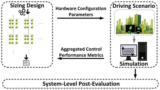
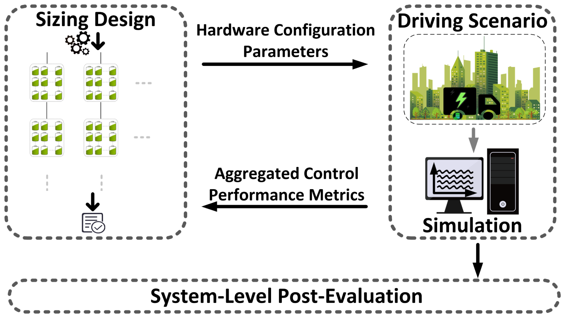
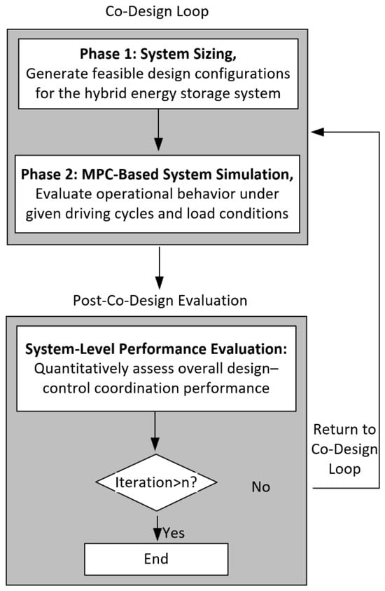
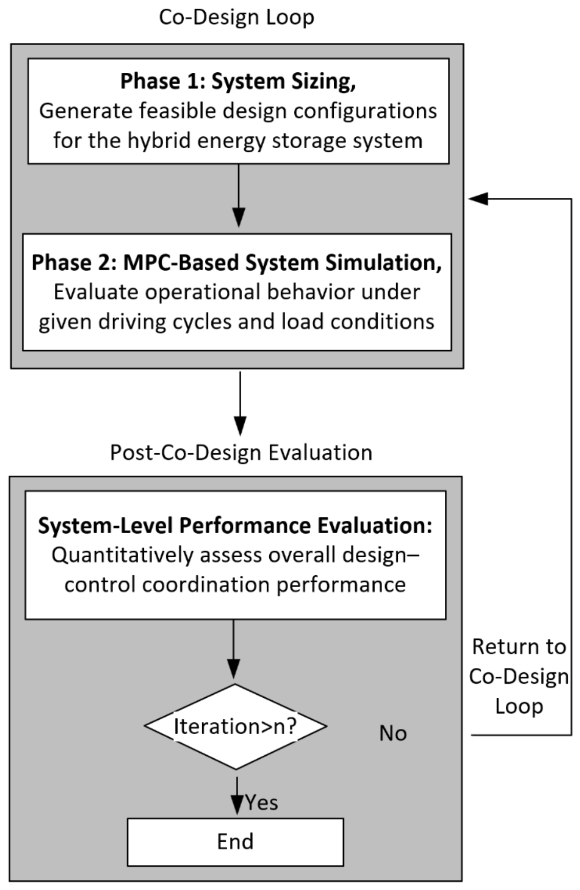
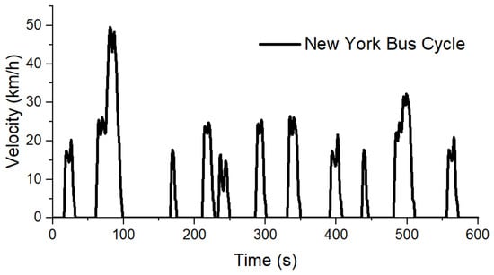
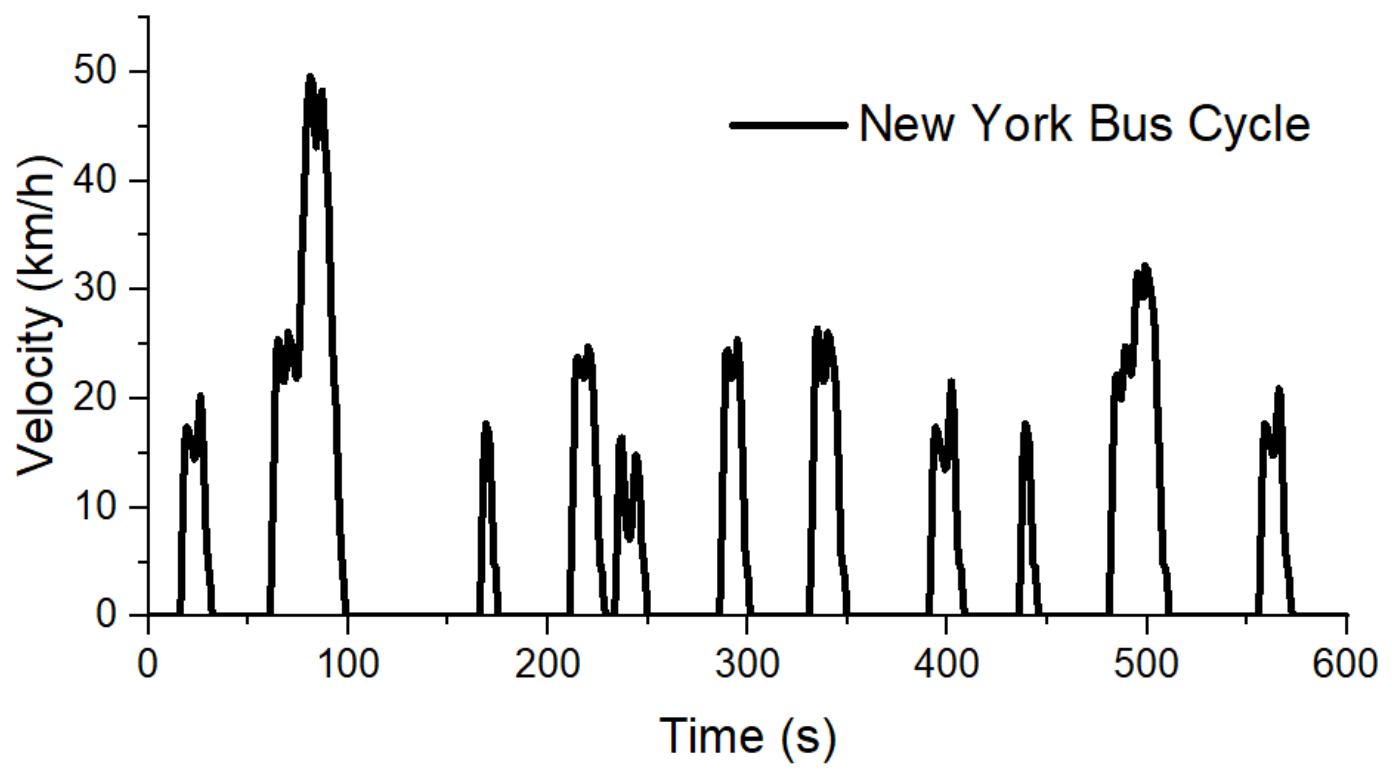
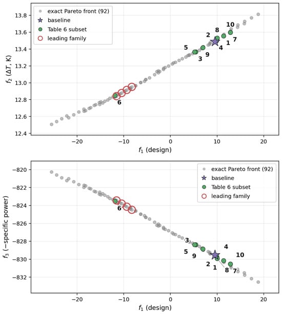
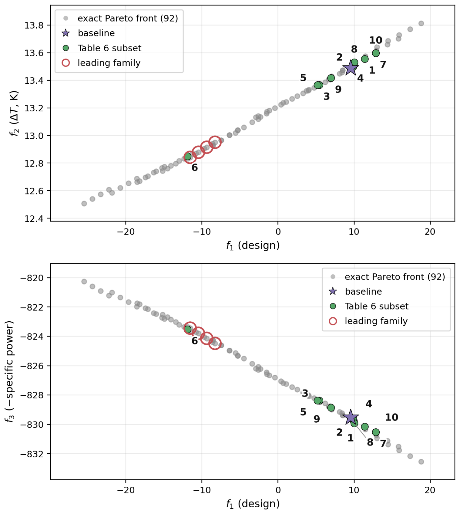
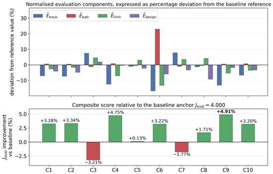
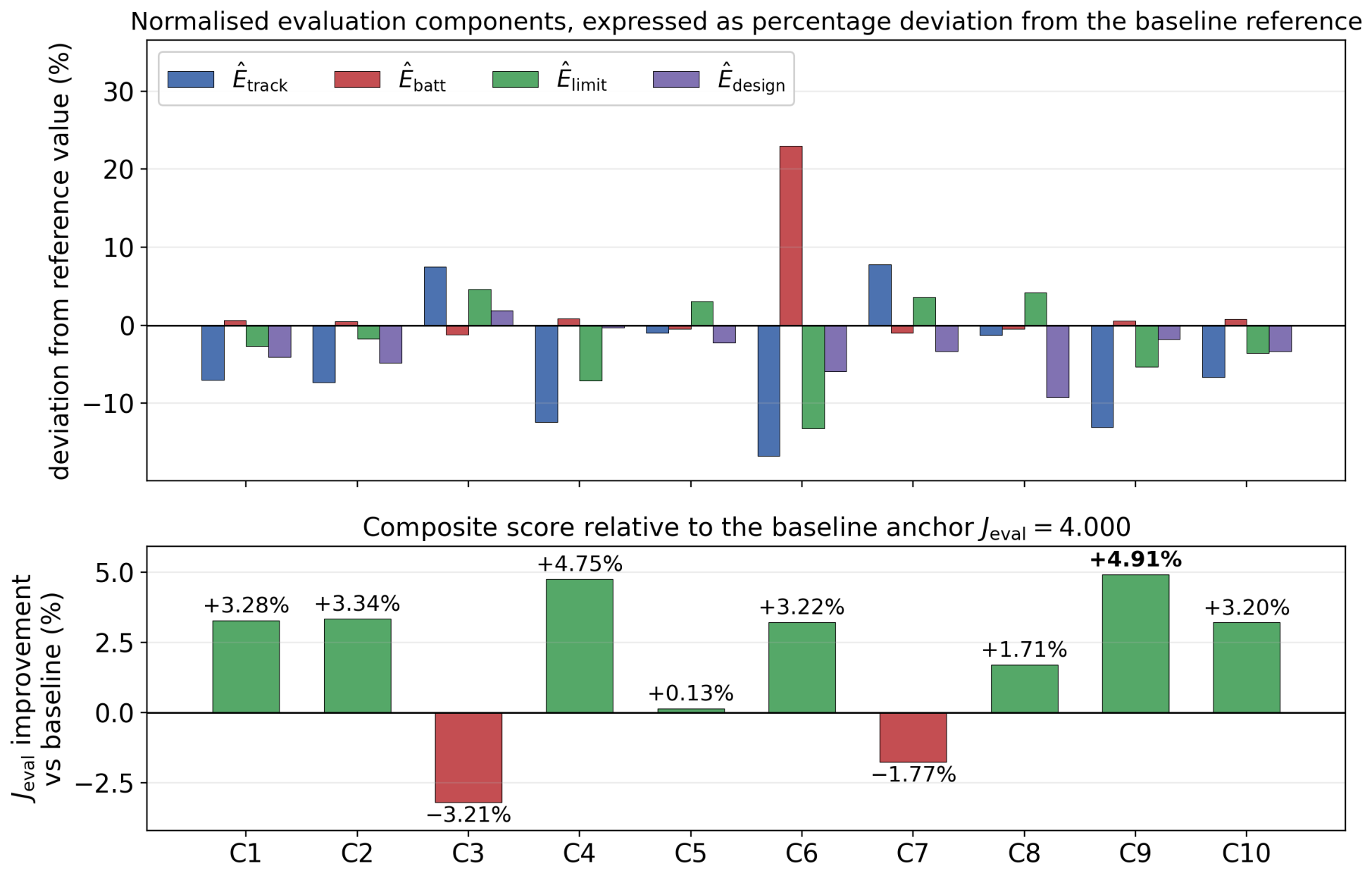
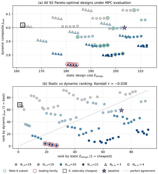
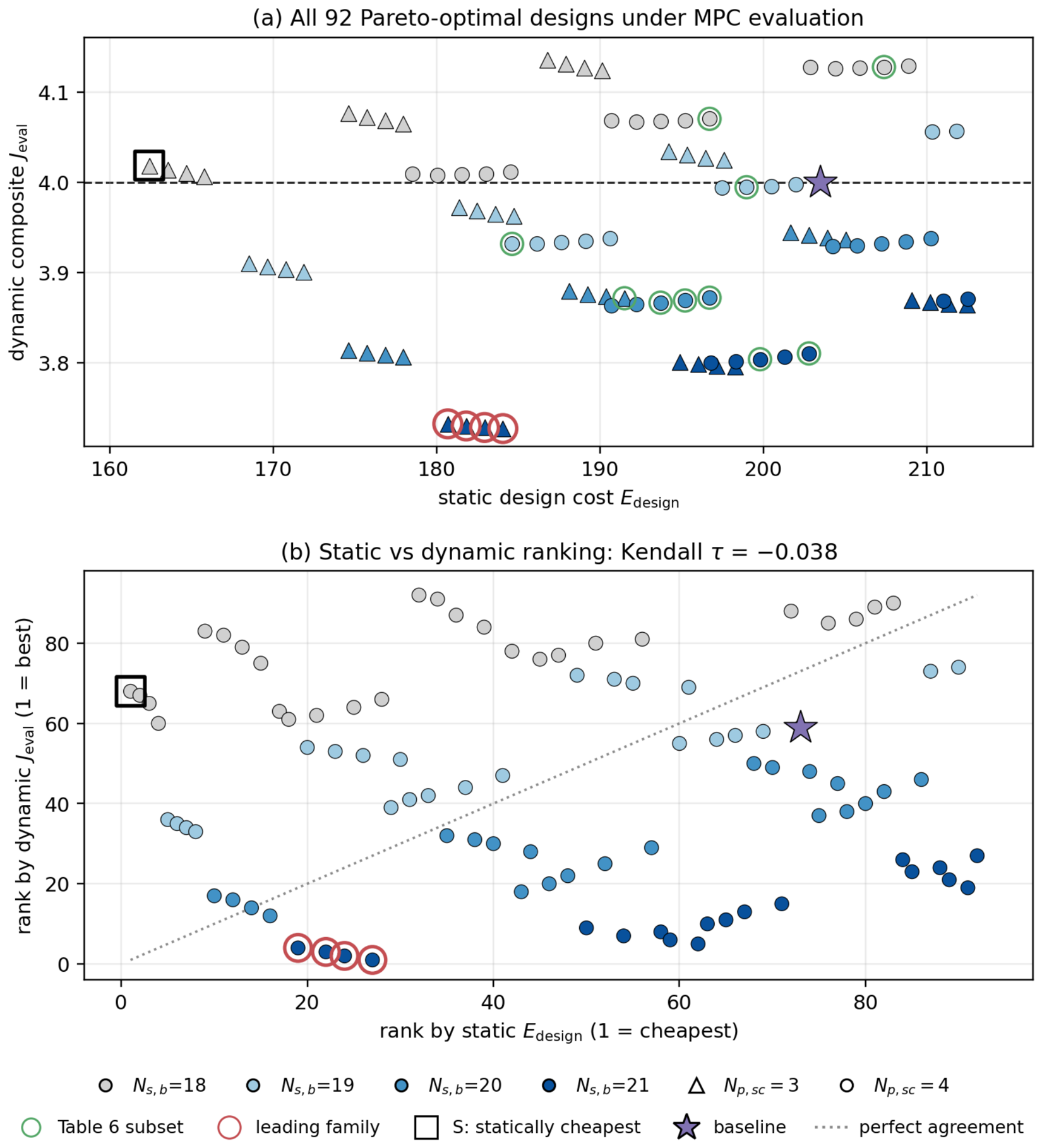
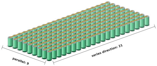
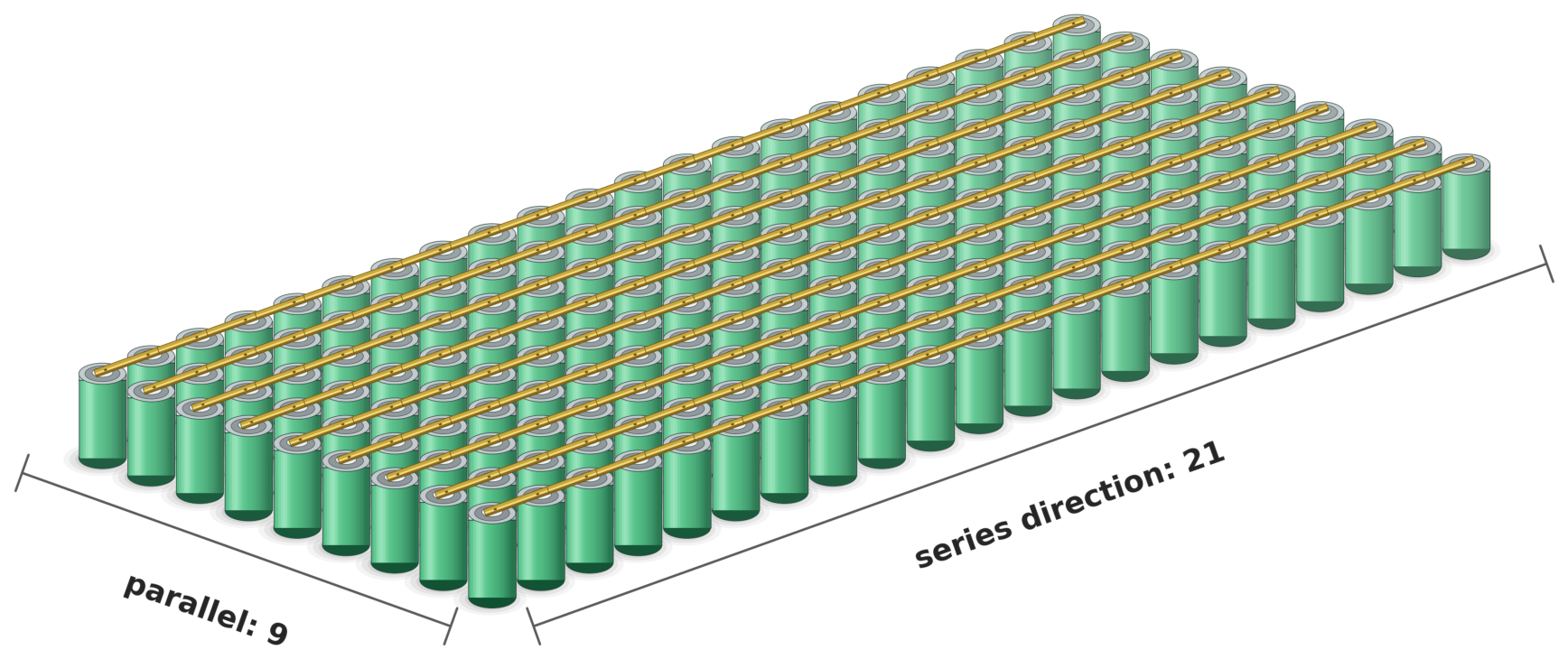
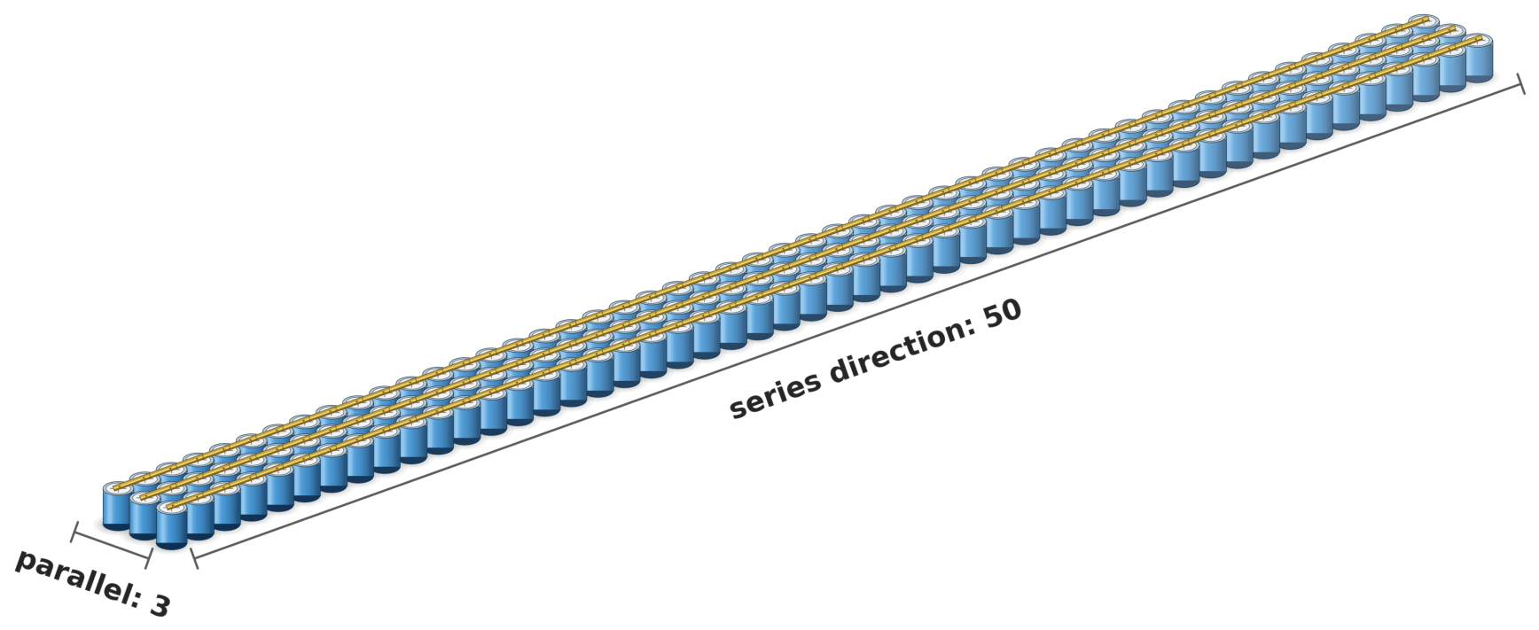
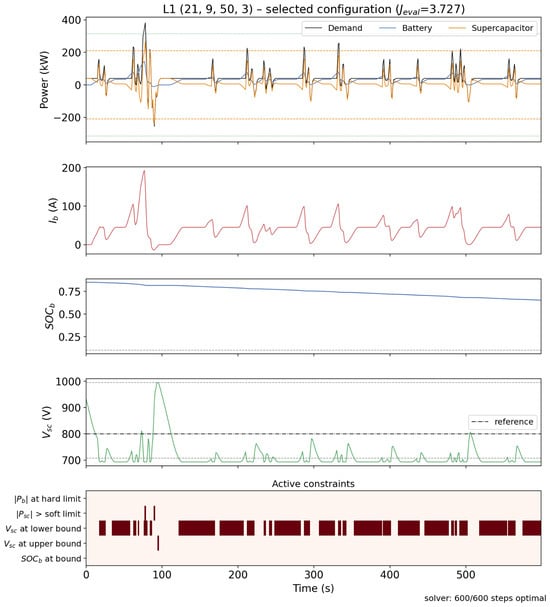
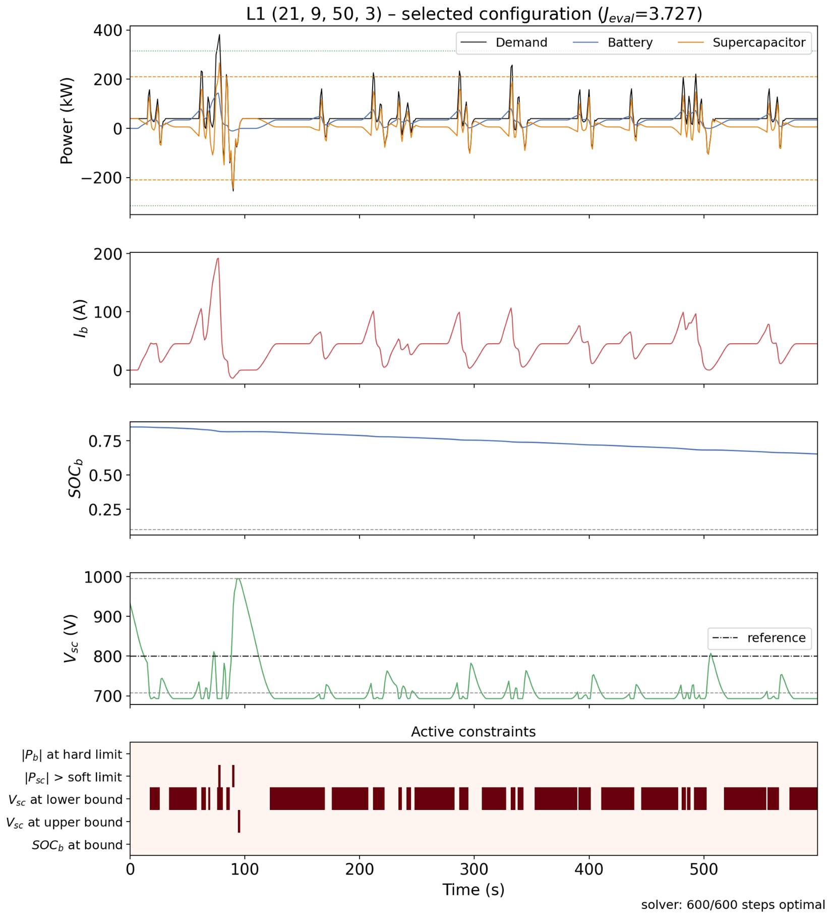
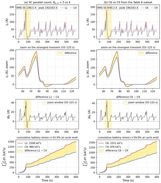
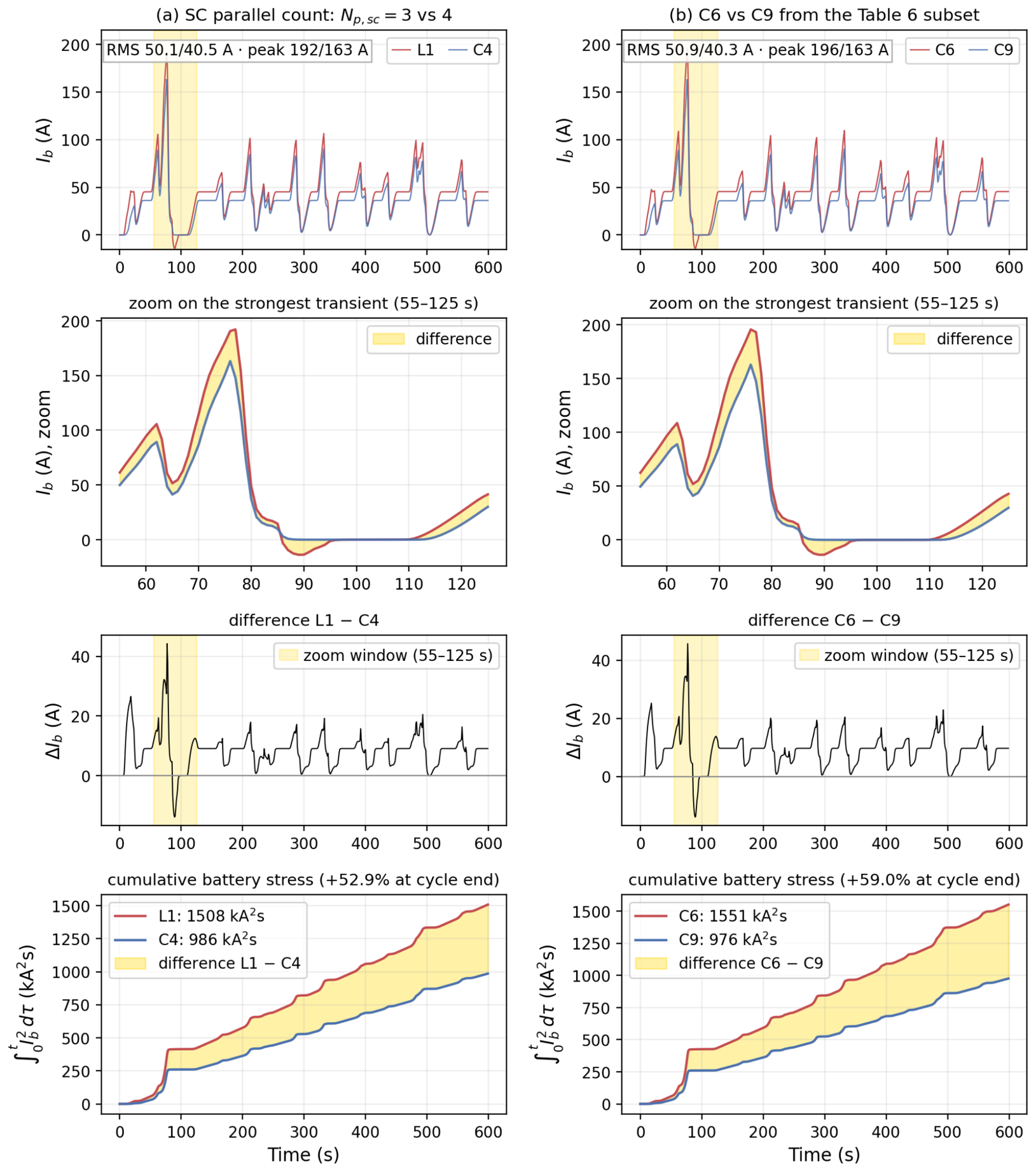
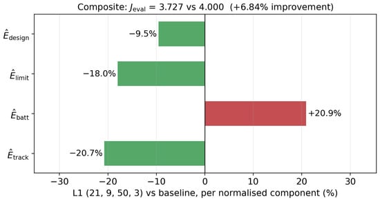
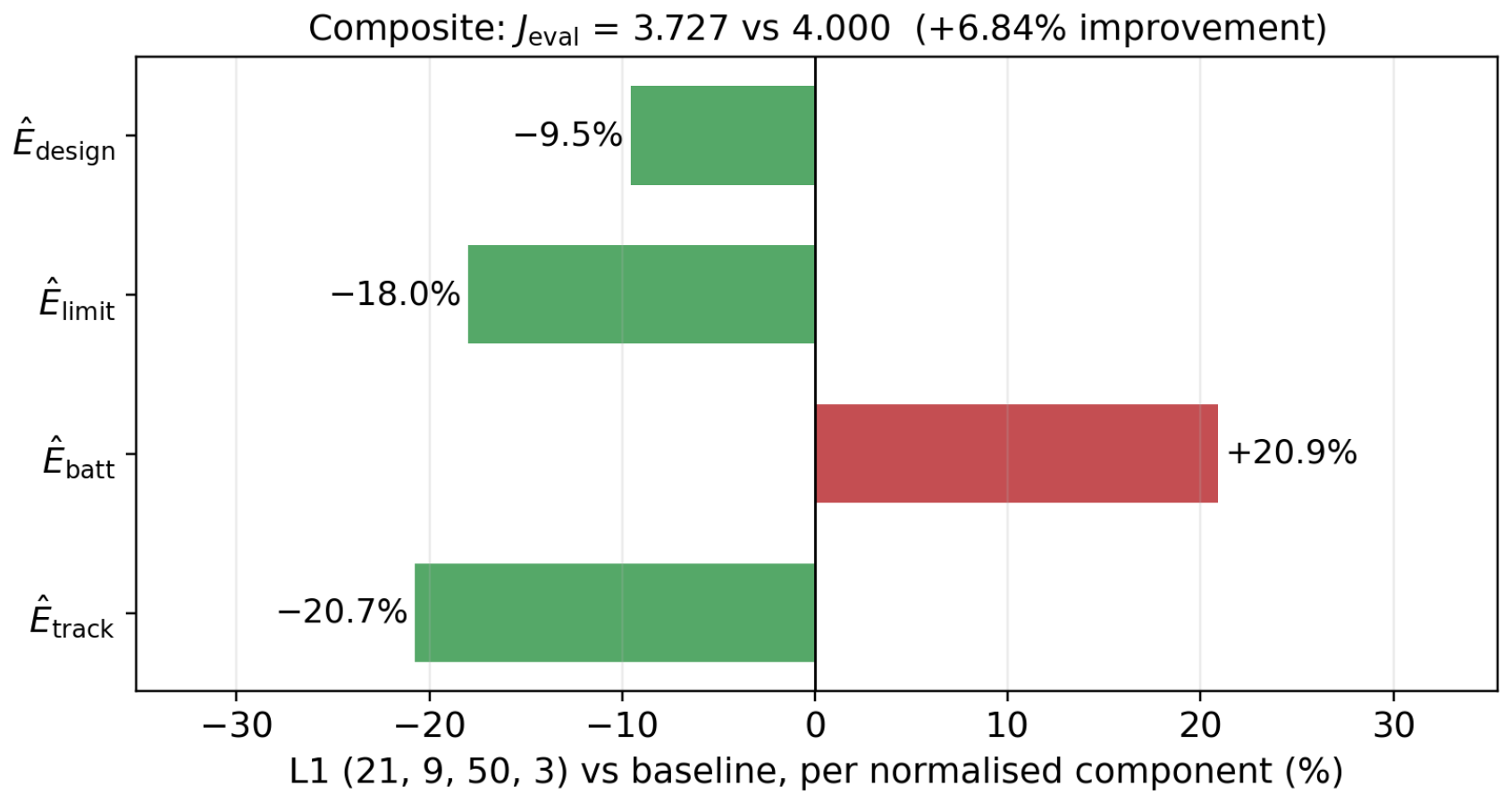
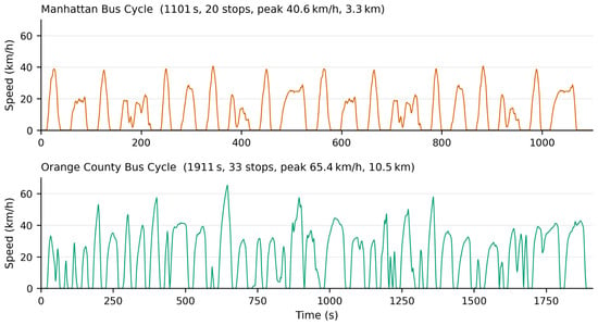
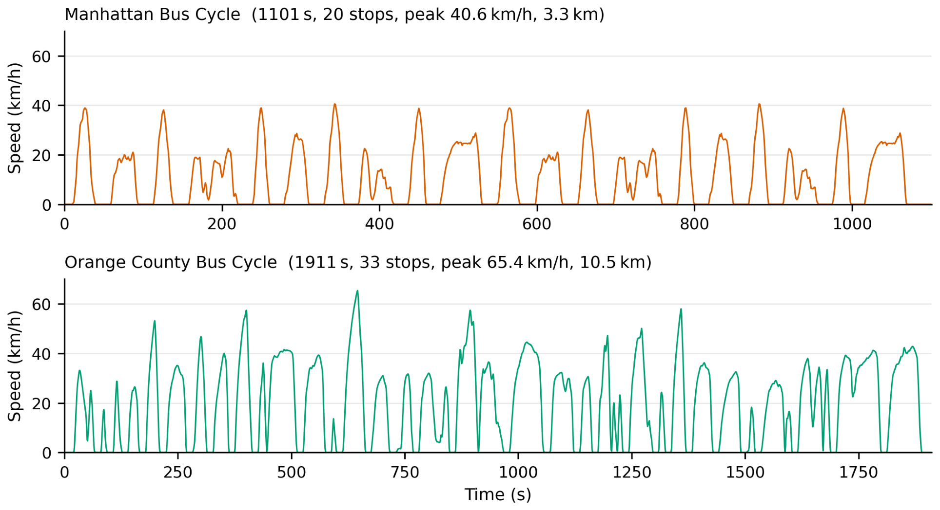
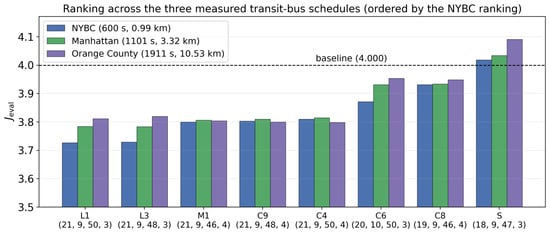

Disclaimer/Publisher’s Note: The statements, opinions and data contained in all publications are solely those of the individual author(s) and contributor(s) and not of MDPI and/or the editor(s). MDPI and/or the editor(s) disclaim responsibility for any injury to people or property resulting from any ideas, methods, instructions or products referred to in the content. |
© 2026 by the authors. Licensee MDPI, Basel, Switzerland. This article is an open access article distributed under the terms and conditions of the Creative Commons Attribution (CC BY) license.