MSFormer: Multi-Scale Transformer for Robust Fault Diagnosis of Machines Under Complex Conditions

Abstract

In rotating machinery monitoring, obtaining highly discriminative fault features from complex vibration signals remains a significant challenge for deep learning-based diagnostic models. In this paper, a novel intelligent fault diagnosis method named MSFormer is proposed. The MSFormer incorporates a parallel multi-scale Convolutional Neural Network (CNN) architecture and hierarchical Transformer modules to comprehensively process 1D vibration signals. By utilizing varying kernel sizes, the multi-scale CNN extracts both high-frequency local transient impulses and low-frequency global degradation trends. Subsequently, the Transformer modules are employed to model the long-range dependencies within the extracted feature sequences, effectively mitigating the interference of environmental noise. Extensive experiments are conducted on bearing fault experimental data to evaluate the proposed method. Four state-of-the-art models are compared under the same experimental settings. Quantitative metrics and qualitative tools are utilized for comprehensive evaluation. Experimental results indicate that MSFormer achieves a 92.67% accuracy, 92.54% F1-score, and 93.22% precision, demonstrating significant superiority. MSFormer provides a powerful and precise intelligent solution for mechanical fault diagnosis.

1. Introduction

At the heart of contemporary industrial systems are the components of rotating machinery, especially rolling bearings. Since unforeseen structural deterioration can cause catastrophic economic damages and extreme safety risks, precise and timely fault detection has become a priority research topic.

In the early days, conventional fault diagnosis used a large number of signal processing methods based on experience, and empirical mode decomposition and wavelet transform [1,2] were devised as methods to extract the frequencies of the defect. In order to reduce human intervention, a traditional machine learning model [3,4] was later provided to automatically determine the type of fault. In the fast development of deep learning, the use of standard convolutional neural networks (CNNs) [5,6] has been common to automatically discover discriminative features of raw monitoring data. However, non-stationary vibration signals are inherent in real world industrial environments, which are dynamic and open in nature, and as such, mechanical equipment would produce non-stationary vibration signals under different operating conditions. This operational variability is a very serious exacerbation of the lack of annotated fault data, becoming a very serious challenge to the possibility of reliable diagnosis with very limited sample sizes. To specifically tackle this data scarcity challenge, recent studies have attempted to integrate domain expertise. For example, multi-task dynamic learning informed by prior knowledge [7] and self supervised feature learning augmented with prior knowledge [8] have been successfully developed to improve machine fault diagnosis by a few shots.

To address these issues, many sophisticated deep learning models have been developed. First, intelligent diagnosis systems based on deep belief networks [9] and sparse auto encoders [10] were created to learn latent characteristic representations of complex signals. Recurrent neural networks (RNNs) [11] and long short-term memory (LSTM) networks [12] were used to model sequential patterns in order to track the temporal changes inherent in vibration data. In addition, attention-based CNNs [13] and deep residual learning networks [14] were developed that focused on informative fault properties and avoided irrelevant variations. In the case of multi-sensor systems, graph convolutional networks [15] and capsule networks [16] were proposed to increase the synthesis of spatial and temporal attributes. Unsupervised domain adaptation (UDA) techniques [17] and deep transfer learning networks [18] also tried to reduce the gap in distributions between the two domains to maintain performance in the context of variable working conditions. In particular, Zhang et al. [19] suggested an RNN-based diagnostic algorithm that detects the type of faults by 1D-to-2D conversion of the vibration signals of the time series, and adding Gated Recurrent Units (GRUs), although this is a required 1D-to-2D conversion, which breaks the physical continuity of time-series data and introduces excessive computational redundancy. To alleviate the spatial and temporal trade-off, multi-branch CNNs [20] and dilated convolutional networks [21] were developed to directly process raw signals. Most recently, vanilla Transformer models [22] have proven themselves to have superior abilities in parallel long-range temporal dependencies. As an example, Ding et al. [23] developed a time frequency Transformer (TFT) model that is motivated by the self-attention mechanism to extract high-dimensional abstractions of time frequency representations (TFRs), although this method is again largely reliant on complex manual TFR computations. In order to increase the cross-domain robustness, adversarial domain adaptation networks [24] and feature disentanglement auto encoders [25] were investigated to isolate fault features and operating conditions. In addition, Zhao et al. [26] suggested a semi-supervised mutual assistance domain generalization (SemiDGFD) network in order to achieve multi-domain generalization with single-source annotations. However, those domain generalization networks [27] and meta-learning diagnostic schemes [28] remain strongly dependent on auxiliary data or complicated pseudo-labeling, and are thus extremely vulnerable to severe overfitting or optimization failure in few-shot regimes. Lastly, Chen et al. [29] suggested a bearing fault diagnosis mechanism that uses a multi-scale CNN and LSTM model to automatically extract multi-frequency features; the sequentiality of the LSTM limits the inference rate, and its use of signal downsampling risks the loss of important high-frequency transient fault features.

A new end-to-end intelligent fault diagnosis architecture called MSFormer is introduced in this paper. In a strictly constrained single-domain setup, the MSFormer integrates a parallel multi-scale 1D CNN with hierarchical Transformer encoders in a sophisticated feature fusion mechanism. In particular, the multi-scale 1D CNN leverages different kernel sizes to implicitly learn high-frequency local transient impulses and low-frequency global degradation patterns using raw 1D vibration signals without any prior information loss. Lightweight Transformer encoders are then presented to independently model long-range global dependencies in the extracted feature sequences, which effectively suppresses intricate industrial background noise. This architecture does not need to use conventional statistical fusion ensembles, or any elaborate geometric distribution alignment loss terms, and inherently learns superior domain-invariant representations using only the internal feature mining motivation of the network.

Unlike conventional hybrid diagnostic frameworks that typically employ a serial stacking strategy where a single-scale CNN is followed by a Transformer encoder, the proposed MSFormer adopts a parallel multi-scale architecture that facilitates the simultaneous extraction of multi-granular features. This paradigm shift prevents the feature smoothing effect which often occurs when local transient impulses are flattened prematurely in serial structures. Furthermore, because the framework delegates independent Transformer encoder modules to each convolutional branch, it preserves the hierarchical synergy between local fine-grained details and long-range global dependencies, which effectively establishes a robust feature disentanglement mechanism that resolves subtle fault severities sharing identical kinematic carrier frequencies. Feature disentanglement is defined as the model’s autonomous capability to isolate underlying physical fault features from complex, noise-corrupted vibration flows.

In summary, the core academic contributions of this paper are outlined as follows:

• A novel end-to-end hybrid diagnostic architecture integrating the local feature extraction advantages of multi-scale 1D CNNs with the global parallel temporal modeling capabilities of Transformers is proposed to achieve robust diagnosis in complex environments.
• MSFormer eliminates the prerequisite for cumbersome 1D-to-2D signal preprocessing and bloated domain alignment or feature decoupling mechanisms, establishing a pure and highly data-efficient 1D streaming paradigm.
• The MSFormer framework resolves overlapping fault severities that share identical kinematic carrier frequencies, a task where traditional spectral analysis and baseline deep learning models frequently fail.
• Extensive comparative experiments against state-of-the-art diagnostic models under a rigorous setting demonstrate the superiority of the proposed framework in both diagnostic accuracy and stability.
• The internal mechanisms of MSFormer are thoroughly analyzed via quantitative confusion matrices and qualitative t-SNE clustering visualizations, with ablation studies further confirming the indispensableness of both the multi-scale convolutional branches and Transformer encoders for constructing excellent intra-class compactness and inter-class separability.

The remainder of this paper is organized as follows. Section 2 details the specific network architecture of the proposed MSFormer, which includes the design mechanism of the multi-scale 1D CNN and the internal components of the hierarchical Transformer encoder. Section 3 introduces the dataset, sample-construction procedure, comparative methods, implementation settings, and evaluation metrics. Section 4 presents and discusses the diagnostic results, stability analysis, confusion matrices, t-SNE visualizations, ablation studies, computational efficiency, and limitations. Finally, Section 5 concludes the paper and outlines future research directions.

2. Proposed Method

The proposed MSFormer architecture is an end-to-end intelligent diagnosis framework. It takes raw 1D vibration signals as input and outputs the predicted health condition of the machinery. The model comprises three fundamental units: a parallel multi-scale feature extraction unit, a hierarchical Transformer encoding unit, and a feature fusion classification head.

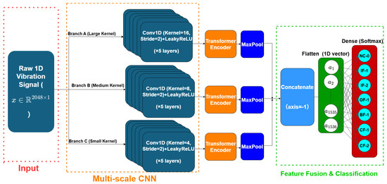
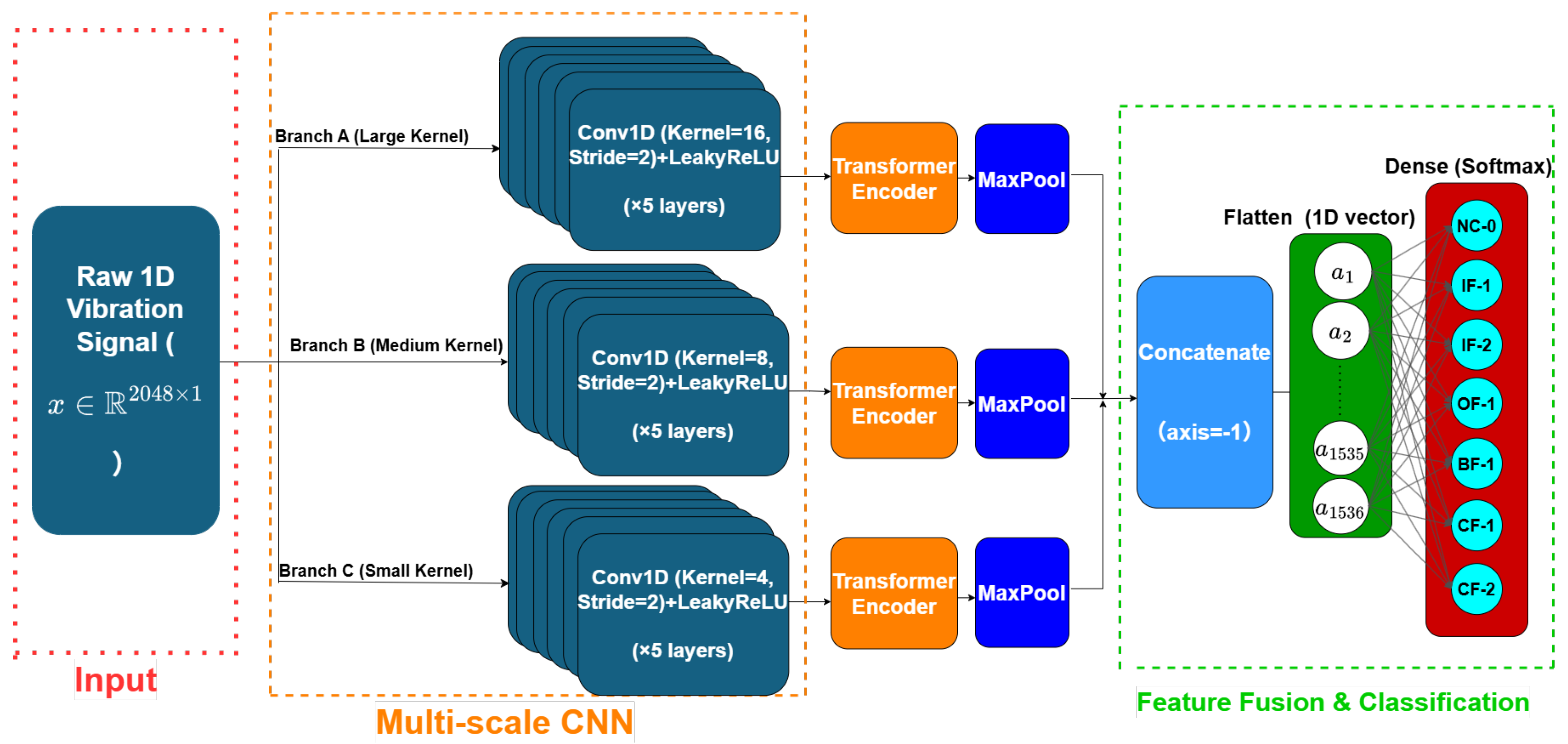
The overall architecture of the proposed MSFormer framework is delineated in Figure 1. Operating as an end-to-end intelligent diagnostic network, the framework fundamentally comprises three progressive stages: the multi-scale convolutional feature extraction, the hierarchical Transformer encoder module, and the feature fusion classification head.

Figure 1. The overall architecture of the proposed MSFormer. The network comprises a multi-scale convolutional feature extraction and a hierarchical Transformer encoder module.

Specifically, the raw 1D vibration signal, denoted as $x\in {\mathbb{R}}^{2048\times 1}$, is initially fed into the input layer. To extract multi-granular temporal frequency representations under restricted training data regimes, the input is processed simultaneously through three parallel branches configured with varying receptive fields: Branch A (Large Kernel, $k=16$), Branch B (Medium Kernel, $k=8$), and Branch C (Small Kernel, $k=4$). Within each independent branch, after the first initial input convolution, a stack of 5 identical 1D convolutional layers with LeakyReLU activation and a stride of 2 is employed to deeply extract local features while gradually reducing the spatial dimension.

Thereafter, instead of utilizing early structural fusion, the abstract feature sequences produced by each branch are directly propagated into their respective, independent Transformer Encoder modules to model long-range temporal dependencies and attenuate severe environmental noise. To further compress the refined feature sequences and distill the dominant diagnostic information, a MaxPooling layer is tightly appended after each Transformer encoder.

In the final feature fusion and classification phase, the robust multi-scale features from the three channels are horizontally combined via a concatenation layer along the channel dimension (Concatenate, axis = −1). The fused multiscale representation tensor is then flattened into a 1D vector comprising exactly 1536 feature elements, with each neuron encapsulating cross-scale global semantics. Ultimately, these 1536 flattened nodes are projected through a fully connected dense layer utilizing the Softmax activation function to yield the predicted probability distribution across the 7 mechanical health conditions, including normal condition, two severities of inner race faults, outer race fault, ball fault, and two severities of cage faults.

2.1. Multi-Scale Feature Extraction

To capture fault impact characteristics across different frequency resolutions, three parallel convolutional branches (Branch A, B, and C) are utilized. The raw 1D vibration signal, denoted as $X\in {\mathbb{R}}^{L\times 1}$ (where $L=2048$ is the data length), is processed by initial convolution layers with varying kernel sizes of 16, 8, and 4, respectively. Large kernels are responsible for global low-frequency components, while small kernels capture high-frequency local transients. For a 1D convolutional layer l, the output sequence $y^l$ is computed as:

$$y_i^l=f\left({\displaystyle \sum _{j=1}^K}{w}_j^l·x_{i\times s+j}^{l-1}+b^l\right)$$

(1)

where $w^l$ is the convolution kernel of size K, $x^{l-1}$ is the input from the previous layer, s is the stride, and $b^l$ is the bias term. To enhance the non-linear expression while preventing the dying ReLU problem, a LeakyReLU activation function is applied after the convolutions:

$$f\left(x\right)=\left\{\begin{array}{cc}x,\hfill & \mathrm{if}x>0\hfill \\ \alpha x,\hfill & \mathrm{if}x\le 0\hfill \end{array}\right.$$

(2)

where the negative slope coefficient $\alpha$ is set to 0.2. Following the activation, a MaxPooling layer is utilized to downsample the feature maps, reducing computational complexity and extracting dominant features:

$$p_i^l=\underset{j\in W}{max}{y}_{i\times s+j}^l$$

(3)

where W is the pooling window size (set to 2). Each branch consists of 6 stacked Conv1D LeakyReLU MaxPooling blocks, gradually reducing the spatial dimension while increasing the channel depth to 256.

2.2. Transformer Encoding Module

The abstract feature sequences produced by the CNN of the three branches are subsequently mapped into Transformer Encoders. The Transformer models the global dependencies within the sequence through the Multi-Head Self Attention (MHSA) mechanism. For the input feature sequence $Z\in {\mathbb{R}}^{N\times D}$, it is first linearly projected into Queries (Q), Keys (K), and Values (V):

$$Q=Z{W}_Q,K=Z{W}_K,V=Z{W}_V$$

(4)

where $W_Q,W_K,W_V$ are learnable weight matrices. The scaled dot product attention is formulated as:

$$\mathrm{Attention}(Q,K,V)=\mathrm{Softmax}\left({\displaystyle \frac{Q{K}^T}{\sqrt{d_k}}}\right)V$$

(5)

where $d_k$ is the dimension of the keys. To jointly attend to information from different representation subspaces, MHSA is applied:

$$\mathrm{MHSA}\left(Z\right)=\mathrm{Concat}({\mathrm{head}}_1,{\mathrm{head}}_2,\dots ,{\mathrm{head}}_h)W_O$$

(6)

$${\mathrm{head}}_i=\mathrm{Attention}(Z{W}_{Q_i},Z{W}_{K_i},Z{W}_{V_i})$$

(7)

where $h=2$ is the number of heads, and $W_O$ is the output projection matrix. The Transformer Encoder incorporates residual connections and Layer Normalization (LN):

$$Z^{\prime }=\mathrm{LN}(\mathrm{MHSA}\left(Z\right)+Z)$$

(8)

$$Z_{out}=\mathrm{LN}(\mathrm{FFN}\left(Z^{\prime }\right)+Z^{\prime })$$

(9)

where the Feed Forward Network (FFN) consists of two dense layers with intermediate ReLU activation. A dropout rate of 0.1 is adopted to prevent overfitting. Finally, an additional MaxPooling layer is applied to the output of the Transformer Encoder.

2.3. Feature Fusion and Classification

After deep semantic processing, the robust features from Branches A, B, and C are concatenated along the channel dimension to form a comprehensive multi-scale global feature representation:

$$F_{fusion}=\mathrm{Concat}(Z_{A\_out},Z_{B\_out},Z_{C\_out})$$

(10)

This fused feature tensor is flattened into a 1D vector and passed through a fully connected dense layer with a Softmax activation function. The final probability distribution for the $C=7$ health conditions is computed as:

$$\widehat{Y}=\mathrm{Softmax}(W_{cls}{F}_{flatten}+b_{cls})$$

(11)

where $W_{cls}$ and $b_{cls}$ are the weights and biases of the classification layer, respectively.

3. Experimental Setup and Evaluation Criteria

3.1. Experimental and Data Description

To verify the efficiency and strength of the suggested MSFormer, the University of Ottawa (UO) bearing dataset is used in this research. Therefore, the proposed method can be confirmed using the rolling bearing experimental data. Detailed information regarding the structural configuration of the bearing test rig, the experimental fault simulation procedures, the specific bearing types (NSK 6203ZZ and FAFNIR 203KD), the data collection process, the sensor layout, data acquisition system (National Instruments USB-6212, National Instruments Corporation, Austin, TX, USA), and sampling configurations (42,000 Hz) were conducted under controlled load and speed conditions to ensure experimental consistency, which can be found in the original dataset documentation [30]. This experiment has the dataset systematically set to seven different health states to model real-world bearing degradation conditions. Such states include a healthy base, and various fault modes with different locations and magnitudes: Normal Condition (NC−0), Inner Race Fault Level 1 (IF−1), Inner Race Fault Level 2 (IF−2), Outer Race Fault (OF−1), Ball Fault (BF−1), Cage Fault Level 1 (CF−1), and Cage Fault Level 2 (CF−2).

The bearing data is categorized based on the standard naming convention of the University of Ottawa dataset. Specifically, file labels formatted as Letter-Number-1 correspond to the Developing fault condition (IF-1), while those formatted as Letter-Number-2 represent the Faulty condition (IF-2). This systematic labeling ensures a clear distinction between varying severity levels of the inner race faults for the MSFormer diagnostic model.

For each of the above bearing conditions, two original vibration records were selected. Each record was divided into 200 consecutive non-overlapping segments, with each segment containing 2048 sampling points. Therefore, 400 samples were constructed for each condition, resulting in 2800 samples in total. At the sampling frequency of 42 kHz, each input segment corresponds to approximately 48.76 ms of vibration data. The raw one-dimensional segments were directly used as the model inputs without manually extracting statistical or spectral features.

In each experimental trial, 10 samples from each condition were randomly selected for training, while the remaining 390 samples per condition were used for testing. Thus, each trial contained 70 training samples and 2730 test samples. This random holdout procedure was repeated ten times using different sample selections. The ground truth of each segment was defined as the experimentally specified condition label inherited from its source record. The predicted condition was determined by the class associated with the maximum Softmax probability and was compared directly with the corresponding ground-truth label. Therefore, no reference vibration waveform or manually defined fault-frequency threshold was used to calculate the classification performance.

From the perspective of bearing kinematics, these localized structural defects generate deterministic recurring impact frequencies. Based on the classical geometric formulations of rolling-element bearings, the theoretical fault characteristic frequencies for the inner race ($BPFI$), outer race ($BPFO$), ball ($BSF$), and cage ($FTF$) are mathematically defined as follows:

$$BPFI={\displaystyle \frac{Z}{2}}·f_r·\left(1+{\displaystyle \frac{d}{D}}\cos \alpha \right)$$

(12)

$$BPFO={\displaystyle \frac{Z}{2}}·f_r·\left(1-{\displaystyle \frac{d}{D}}\cos \alpha \right)$$

(13)

$$BSF={\displaystyle \frac{D}{2d}}·f_r·\left(1-{\left({\displaystyle \frac{d}{D}}\cos \alpha \right)}^2\right)$$

(14)

$$FTF={\displaystyle \frac{1}{2}}·f_r·\left(1-{\displaystyle \frac{d}{D}}\cos \alpha \right)$$

(15)

where Z represents the total number of rolling balls, d denotes the ball diameter, D is the pitch diameter of the bearing configuration, and $\alpha$ stands for the spatial contact angle. The parameter $f_r$ denotes the mechanical shaft rotational frequency governed by the motor speed ($f_r=N/60$, where N is the rotational speed in RPM). Under a specific operational condition, these deterministic frequencies serve as the underlying physical boundaries for the diagnostic networks, as shown in Table 1.

Table 1. Official geometric parameters and the comprehensive list of theoretical fault characteristic frequencies of the UO bearing configuration.

Parameters	Value	Component	Frequency (Hz)
Number of Balls (Z)	8	Shaft Freq ($f_r$)	30.32
Ball Diameter (d)	6.77 mm	Inner Race ($BPFI$)	150.1
Pitch Diameter (D)	28.50 mm	Outer Race ($BPFO$)	92.46
Contact Angle ($\alpha$)	0°	Ball Fault ($BSF$)	60.21
Nominal Speed (N)	1819 RPM	Cage Fault ($FTF$)	11.56

To ensure structural consistency, the dataset is standardized into seven health states, each representing distinct physical degradation characteristics:

• NC-0: Baseline operational state with no identifiable localized defect.
• IF-1, IF-2: IF-1 represents a micro-crack causing low-amplitude high-frequency resonant shocks. IF-2 signifies severe spalling inducing macroscopic mechanical impacts and distinct low-frequency energy shifts.
• OF-1: Standardized localized spalling on the outer ring, producing periodic impact sequences determined by $BPFO$.
• BF-1: Localized surface damage on the rolling elements, characterized by dual-impulse modulations as the ball impacts both the inner and outer races at the $BSF$ frequency.
• CF-1, CF-2: CF-1 corresponds to early-stage plastic deformation or wear, while CF-2 represents catastrophic structural breakage, leading to irregular slip and erratic impact intervals related to $FTF$.

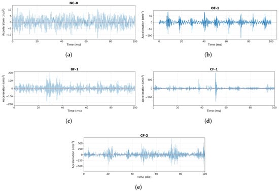
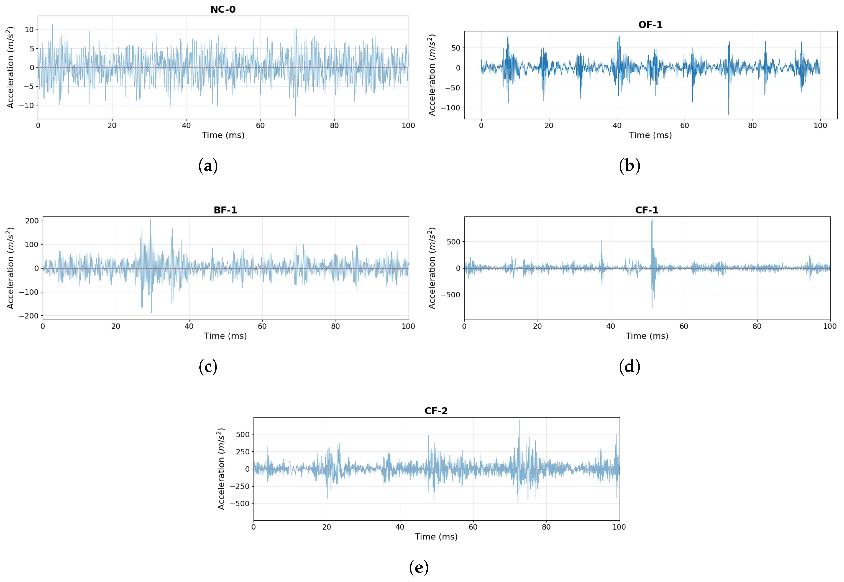
Figure 2 presents time-domain acceleration signals of the remaining bearing conditions, including NC-0, OF-1, BF-1, CF-1, and CF-2. All signals are displayed over the same 100 ms time interval at a sampling frequency of 42 kHz. The normal condition exhibits a comparatively stable vibration response, whereas the fault conditions show different transient fluctuations, impact distributions, and amplitude-modulation patterns.

Figure 2. Representative raw time-domain acceleration signals of the remaining bearing conditions: (a) NC-0, (b) OF-1, (c) BF-1, (d) CF-1, and (e) CF-2.

Because the vibration amplitudes differ substantially among the bearing conditions, the vertical axis of each subplot is independently scaled to clearly reveal its local waveform morphology, while the horizontal time scale remains identical. Therefore, the absolute amplitudes should not be directly compared across different subplots. These representative waveforms are provided only for qualitative visualization and physical interpretation and are not used as reference signals for calculating diagnostic accuracy. The quantitative ground truth is defined by the experimentally specified condition label inherited from each source record.

While fault locations are anchored by their respective kinematic characteristic frequencies, the multi-level severity classification of IF and CF introduces significant diagnostic challenges. Specifically, since sub-level faults occur on the identical bearing component, they share the same theoretical kinematic carrier frequency, rendering standard frequency-domain spectral analysis insufficient for disentanglement.

Although IF-1 and IF-2 share essentially the same BPFI, their measured responses may differ in transient distributions, modulation characteristics, relative harmonic structures, and resonance-band excitation. The instantaneous vibration amplitude is also affected by the selected observation interval, structural transfer path, operating condition, and sensor response. Therefore, a monotonic relationship between the displayed waveform amplitude and the dataset-defined fault-development stage should not be assumed. Similarly, CF-1 and CF-2 share the same FTF, and their differentiation requires the analysis of more comprehensive temporal and modulation-related patterns rather than characteristic-frequency position or instantaneous amplitude alone.

To clarify the diagnostic paradigm, it is important to emphasize that the proposed MSFormer follows a pure end-to-end learning strategy. Unlike conventional methods that rely on explicit manual feature engineering such as Fast Fourier Transform (FFT) or predefined statistical descriptors, MSFormer utilizes raw 1D time-series vibration data ($2048\times 1$) as the direct input. No manually calculated RMS, kurtosis, skewness, crest factor, power-spectrum coefficients, or theoretical BPFI, BPFO, BSF, and FTF values are supplied to the classifier. The theoretical characteristic frequencies are used only for physical interpretation and signal verification.

To effectively disentangle these overlaps, MSFormer employs a hierarchical feature extraction mechanism: first, the multi-scale 1D CNN functions as adaptive data-driven bandpass filter banks, where small kernels ($k=4$) sharpen their receptive fields to lock onto subtle, high-frequency transients of incipient faults (IF-1, CF-1), while large kernels ($k=16$) integrate the massive structural vibration energy jumps characteristic of severe spalling (IF-2, CF-2). Subsequently, the Transformer encoder performs high-level semantic correlation mapping on these multi-scale feature flows, capturing the non-linear modulation patterns and energy hierarchies that allow for precise fine-grained severity diagnosis even when spectral peaks coincide.

3.2. Comparative Methods

To comprehensively assess the excellence and strength of the proposed MSFormer, four state-of-the-art deep learning diagnostic models were chosen as comparison means.

• MCNN: A classical multiscale CNN lacking global dependency modeling [31].
• MCSAT: A multi-channel network combined with BiLevelRoutingAttention [32].
• MRCNN: A model incorporating residual connections into a multi-scale CNN [33].
• TCAC: A complex network combining Channel Attention and Transformer modules but lacking shallow multi-scale fusion [34].

To ensure the reproducibility and transparency of this study, all models were implemented in a unified Python (3.6.4) environment using TensorFlow (2.1.0)/Keras (2.3.1). All dependencies on MATLAB (R2023b) were eliminated during the data processing phase; instead, the original (.mat) data files were directly ingested and processed using the scipy.io library. The model training process was configured with optimized hyperparameters to ensure stable convergence. Specifically, the learning rate was initialized at $1\times {10}^{-3}$ to facilitate optimal gradient updates. The batch size was set to 7 to accommodate the specific input constraints of the 1D signal slices. The LeakyReLU activation function was utilized with a negative slope coefficient of $\alpha =0.2$ across all convolutional layers. All computational benchmarks and model training were conducted on a workstation equipped with an AMD Ryzen 9 7945HX CPU and an NVIDIA RTX 4060 GPU (8GB VRAM). This standardized environment ensures that both computational complexity and inference latency metrics are comparable and reproducible for future research.

3.3. Evaluation Metrics

To gain a comprehensive and objective assessment of the performance of the proposed MSFormer in terms of diagnostic accuracy, feature extraction ability, and robustness of the proposed model in complex settings, a joint set of quantitative and qualitative evaluation measures is implemented in this research.

3.3.1. Quantitative Metrics

The performance of the models in terms of overall classification is measured quantitatively with three main measures: Accuracy, Precision, and F1-Score. For a multi-class fault diagnosis task, these measures are derived using the macroscopic aggregation of the True Positives (TP), False Positives (FP), True Negatives (TN), and False Negatives (FN) of each class. TP denotes samples whose true label and predicted label both correspond to the considered condition; FP denotes samples belonging to other conditions but incorrectly predicted as the considered condition; FN denotes samples belonging to the considered condition but incorrectly predicted as another condition; and TN denotes samples belonging to other conditions and also predicted as conditions other than the considered condition. In this controlled experiment, these quantities are established by comparing the model predictions with the experimentally specified condition labels provided by the University of Ottawa dataset. In practical industrial applications, equivalent ground-truth labels may be established from verified historical maintenance records, inspection results, expert assessments, or post-disassembly examinations.

• Accuracy: Represents the proportion of correctly predicted samples out of the total testing samples. It reflects the overall diagnostic correctness of the model.

  $$Accuracy={\displaystyle \frac{TP+TN}{TP+TN+FP+FN}}$$

  (16)
• Precision: Represents the proportion of true fault samples among all samples predicted as a specific fault type. It measures the model’s ability to avoid false alarms.

  $$Precision={\displaystyle \frac{TP}{TP+FP}}$$

  (17)
• F1-Score: The harmonic mean of Precision and Recall. In scenarios where feature boundaries might be blurred, the F1-Score serves as a more comprehensive metric than Accuracy to evaluate the balanced performance of the model.

  $$F1\text{-}Score=2\times {\displaystyle \frac{Precision\times Recall}{Precision+Recall}}$$

  (18)
• Robustness Evaluation (Standard Deviation):
  Since the diagnosis is highly sensitive to random data splitting and initialization, relying solely on a single experimental result is scientifically insufficient. Therefore, each model undergoes $J=10$ independent cross trials. The Standard Deviation ($SD$) of the evaluation metrics is introduced as a core indicator of model stability and robustness:

  $$SD=\sqrt{{\displaystyle \frac{1}{J}}\sum _{i=1}^J{(x_i-\mu )}^2}$$

  (19)

In addition to the aforementioned comprehensive metrics, the confusion matrix is introduced as a detailed quantitative tool to evaluate the classification performance across specific health conditions. By mapping the predicted categories against the true labels, the confusion matrix provides a granular tabular representation of the diagnostic results. When normalized with respect to the ground-truth class, the diagonal elements represent class-specific recall or true positive rate, rather than overall accuracy, while the off-diagonal elements explicitly quantify the misclassification probabilities between mutually confusing fault categories. This matrix enables a rigorous assessment of the model’s diagnostic sensitivity, particularly when distinguishing faults with varying severities in the same mechanical component.

3.3.2. Qualitative Metrics

To obtain the intuitive understanding of the information of capability of feature extraction and physical process of the proposed MSFormer, a qualitative evaluation process is undertaken along with the quantitative measures. In particular, the t Distributed Stochastic Neighbor Embedding (t-SNE) algorithm is profiled in this research.

Being one of the most popular non-linear dimensionality reduction methods, t-SNE has proven to be very effective for projecting a high-dimensional latent representation in a two-dimensional visual format that can render the local structure of the data. The high-dimensional abstract features produced by the last Flatten layer of the MSFormer are then run through t-SNE to produce a scatter plot during the experimental evaluation phase. This qualitative measure has a clear visualization of the intra-class compactness and inter-class separability of the trained feature distributions. The t-SNE visualization is a first-hand visual demonstration of the model decoupling of features and resistance to environmental noise, by intuitively showing whether the signals of various health conditions are highly clustered or overlap. It should be emphasized that t-SNE is used only for qualitative visualization. The apparent cluster distances, shapes, and local overlaps in the two-dimensional projection should be interpreted together with the confusion matrices and quantitative evaluation metrics.

4. Results and Discussion

This section presents and discusses the experimental results of the proposed MSFormer and the comparative models. The analysis covers overall diagnostic performance, stability, class-wise classification behavior, learned-feature distributions, ablation results, computational efficiency, and the limitations of the present study.

4.1. Diagnosis Results and Discussion

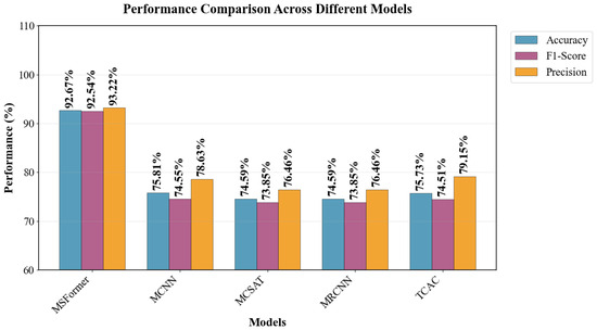
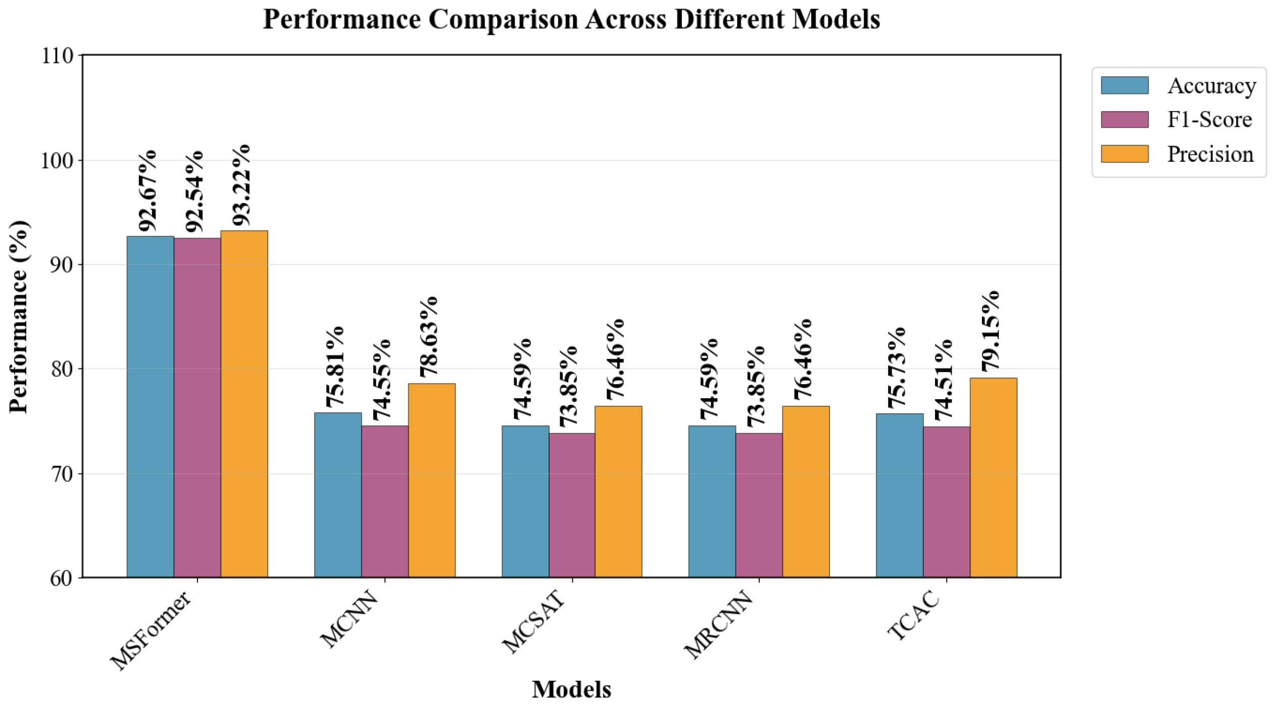
Figure 3 gives a detailed comparison of the performance of each of the five models on three key evaluation measures, namely Accuracy, F1-score, and Precision. The MSFormer, as indicated in the figure, is very effective in terms of performance compared to all other models. The Accuracy of 92.67%, F1-score of 92.54%, and Precision of 93.22% of MSFormer are impressive, given its performance level of more than 92 across all the metrics with only 10 samples per class.

Figure 3. Performance comparison of different diagnostic models.

By contrast, the comparative models have significantly lower performance. The evaluation metrics of the comparative models are mainly concentrated in the 73–79% range. For instance, MCNN yields an Accuracy of 75.81% and an F1-score of 74.55%, performing the best among the baselines but still lagging behind MSFormer by nearly 17%. TCAC achieves an Accuracy of 75.73%, while MCSAT and MRCNN both stall at 74.59%. The overall F1-score and Precision of these baselines remain inferior. The experimental results strongly indicate that relying solely on multi-scale CNNs (MCNN, MRCNN) or isolated attention mechanisms (MCSAT, TCAC) is insufficient for extracting discriminative features. MSFormer offers the best trade-off, showcasing superior and balanced performance by successfully capturing both local transient impulses and global degradation trends.

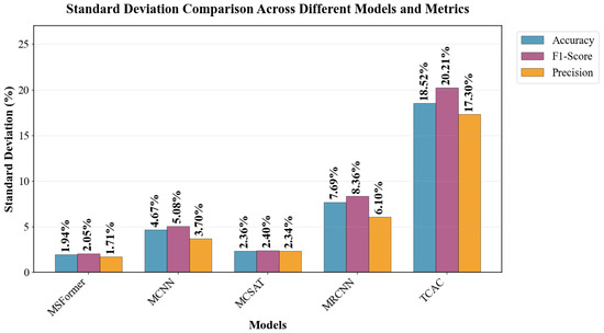
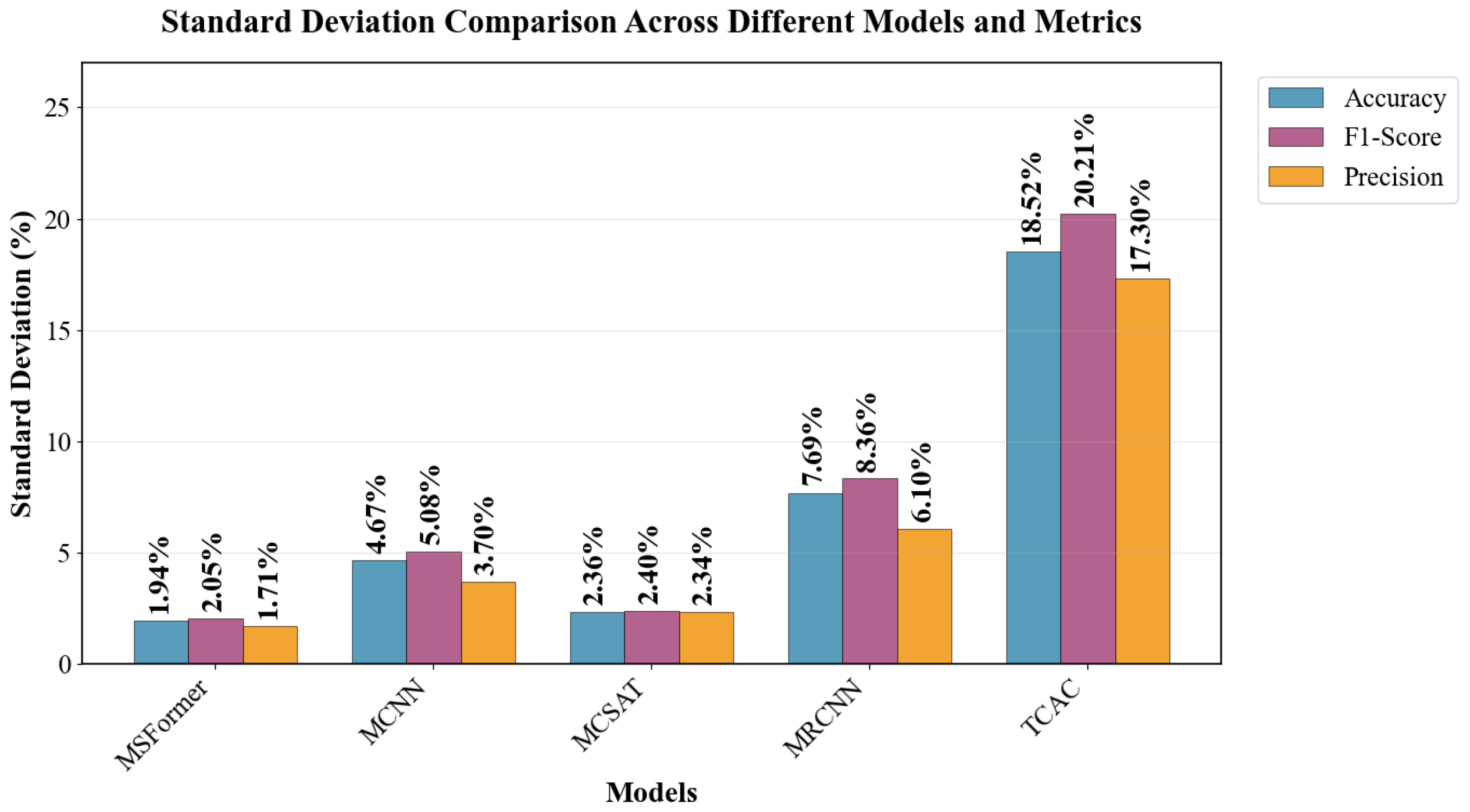
According to the standard deviation comparison across all evaluation metrics, MSFormer consistently demonstrates the highest stability among all models. As illustrated in Figure 4, its standard deviations in Accuracy, F1-Score, and Precision are 1.94%, 2.05%, and 1.71%, respectively, all remaining well below 2.5%. This indicates that the performance of MSFormer is minimally influenced by data variation and maintains strong robustness.

Figure 4. Standard deviation comparison of the proposed MSFormer and comparative baseline models. The consistently low standard deviations of MSFormer across all metrics demonstrate its superior stability and robustness.

In comparison, the remaining models exhibit significantly larger fluctuations. TCAC shows extreme instability. This suggests that the pure Transformer-based structure in TCAC is highly prone to overfitting and severe performance collapse when trained on limited samples without multi-scale inductive biases. MRCNN and MCNN also exhibit moderate variance. Although MCSAT achieves a competitive stability, its overall accuracy is substantially lower than that of MSFormer.

Furthermore, detailed statistical analysis reveals two key findings:

• The F1 Score exhibits the largest error across almost all models, indicating that this metric is the most sensitive to data variations and class imbalances.
• Precision consistently shows the smallest error, indicating relatively stable false-positive rates. Taken together, these results show that MSFormer not only surpasses all baseline models in diagnostic accuracy but also provides the most reliable, consistent, and robust predictive behavior.

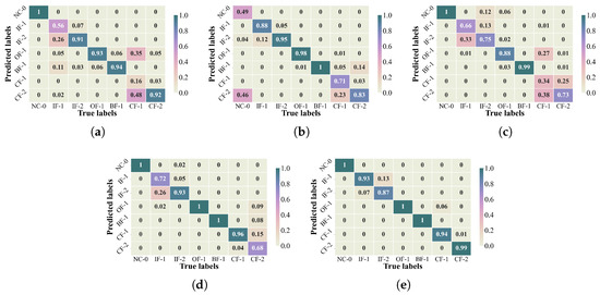
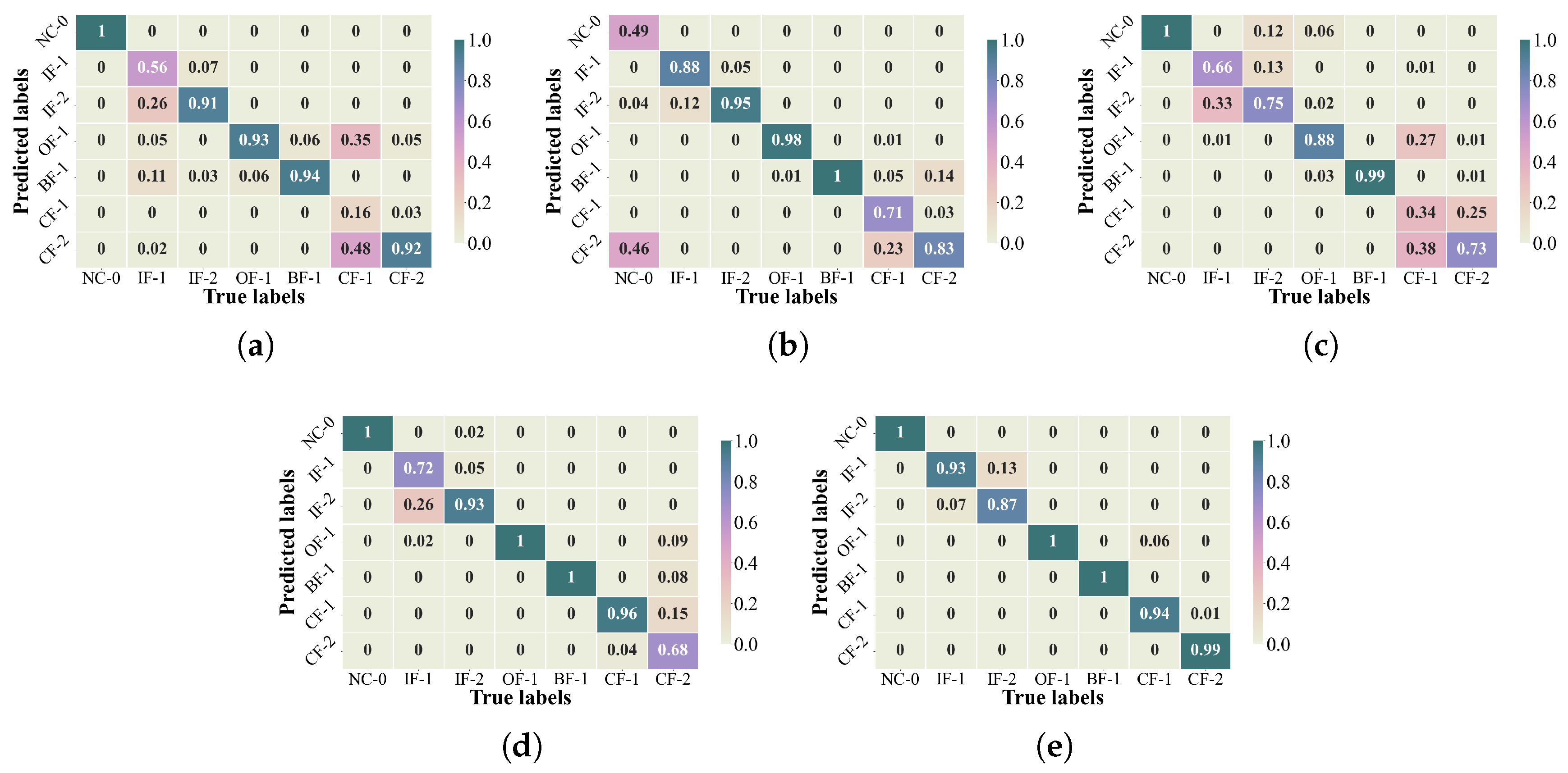
In Figure 5, by comparing the confusion matrices shown from (a) to (e), the fine-grained classification capabilities of the models can be observed. The research found that compared with MSFormer, the baseline models show high rates of mutual misidentification, particularly among fault types with similar physical manifestations.

Figure 5. Confusion matrices of the proposed MSFormer and different baseline models. (a) MCNN, (b) MCSAT, (c) MRCNN, (d) TCAC, and (e) MSFormer.

For instance, the MCNN and MRCNN models show a high rate of misclassifying between IF-1 and IF-2. Moreover, CF-1 is confused with CF-2. They do not indicate confusion between inner-race faults and cage faults. TCAC exhibits the most severe confusion, almost completely failing to distinguish between CF-1 and CF-2 and mistakenly identifying early-stage inner race faults as outer race faults. The MCSAT model performs better than TCAC but still leaves a noticeable gap in classifying IF-2.

Conversely, the experimental results demonstrate that MSFormer achieves the clearest diagonal matrix. It yields a 100% recognition rate for NC-0, OF-1, and BF-1. More importantly, it significantly suppresses the misclassification between IF-1 and IF-2, achieving recognition rates of 0.93 and 0.87, respectively. This demonstrates that MSFormer possesses superior recognition capability for subtle and overlapping fault signatures compared to the other four models.

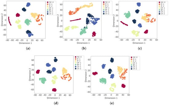
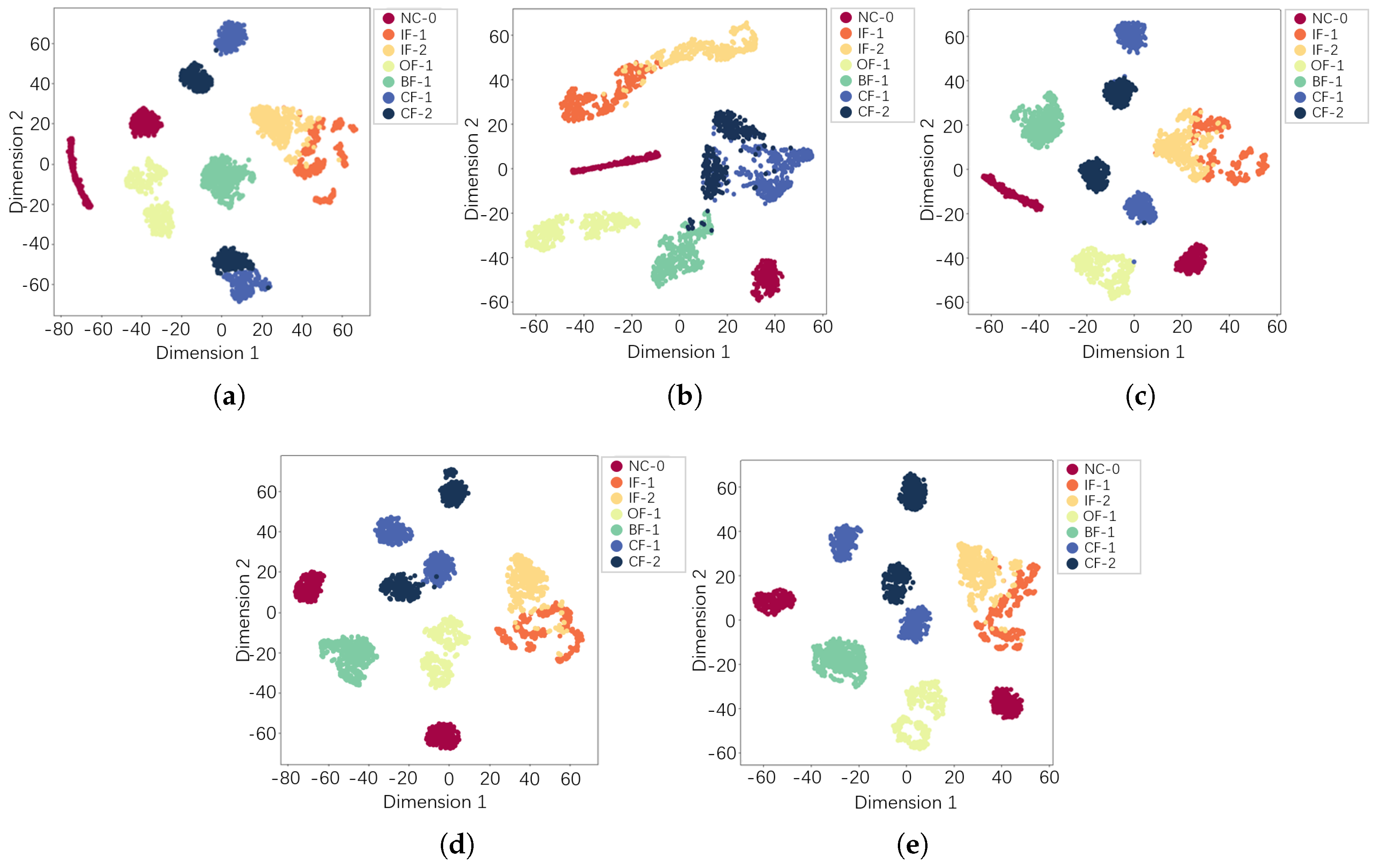
To visualize the feature representations learned by the diagnostic networks, t-SNE was applied to the output of the final feature layer immediately before the Softmax classifier. For MSFormer, this representation corresponds to the 1536-dimensional vector produced by the Flatten layer after multi-scale feature fusion. These dimensions are data-driven latent features jointly learned by the convolutional and Transformer modules, rather than manually defined statistical or spectral indicators. The t-SNE algorithm projects these learned feature vectors into a two-dimensional space to qualitatively assess their intra-class compactness and inter-class separability, as shown in Figure 6. The comparative analysis of the visualization results is as follows:

Figure 6. t-SNE visualizations of the learned feature representations extracted from the penultimate feature layer of different diagnostic networks. (a) MCNN, (b) MCSAT, (c) MRCNN, (d) TCAC, and (e) MSFormer.

MCNN and MCSAT: Generally produce distinguishable clusters for most bearing conditions. However, some class pairs exhibit reduced inter-class margins and limited overlap near their boundaries. In particular, the IF-1 and IF-2 clusters are closely adjacent and show partial boundary overlap, while MCSAT also exhibits local boundary mixing between CF-1 and CF-2. The feature distributions produced by these baseline models are dispersed and show weak cluster compactness.

MRCNN: This model demonstrates an improvement in clustering over MCNN and MCSAT, with more defined boundaries for most fault types. However, notable feature overlap persists between IF-1 and IF-2. Furthermore, the clusters for these two inner race fault categories appear relatively dispersed and exhibit weaker intra-class compactness.

TCAC and MSFormer: Both models achieve clustering performance. MSFormer exhibits superior intra-class compactness for IF-1 and IF-2. Compared to TCAC, which shows more overlap, MSFormer produces more tightly bound clusters, indicating a more consistent feature representation for these challenging fault types. Furthermore, a notable difference in feature distribution is observed in the CF-2 category. While MSFormer maintains a cohesive and dense cluster, TCAC exhibits feature fragmentation, where the CF-2 samples are split into spatially separated sub-clusters. This demonstrates that MSFormer provides higher structural integrity in its learned feature space.

4.2. Ablation Study and Module Contribution Analysis

To analyze the contribution of each key component in the proposed method to performance improvement, ablation experiments were conducted. The comparative methods were constructed as follows.

• Model 1;
  • Model1-A: This model retains only the Transformer module and a single branch A;
  • Model1-B: This model retains only the Transformer module and a single branch B;
  • Model1-C: This model retains only the Transformer module and a single branch C.
• Model 2: This model is a multi-scale CNN model without the Transformer module;
• Model 3: Three models with a CNN model without multi-scale functionality.
  • Model3-A: This model only retains branch A;
  • Model3-B: This model only retains branch B;
  • Model3-C: This model only retains branch C.
• MSFormer.

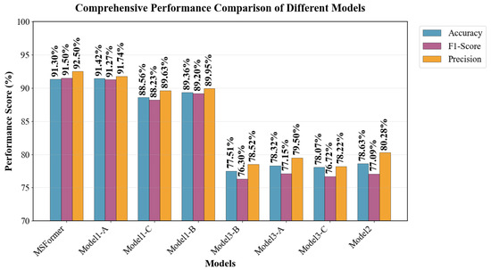
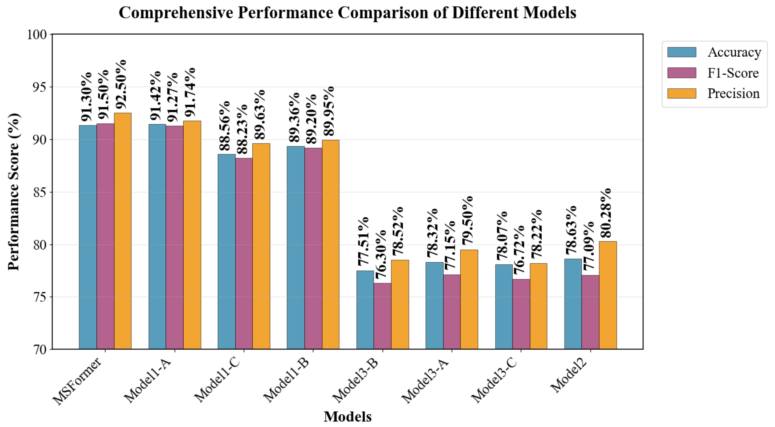
Figure 7 presents a comprehensive comparison of the performance of all models across four evaluation metrics, which include Accuracy, F1-score, Precision, and Recall. As shown in the figure, MSFormer and Model1 series (Model1-A, Model1-C, and Model1-B) outperform the other models. Among them, MSFormer and Model1-A even achieve performance levels above 0.90 on all four metrics. However, MSFormer yields the best overall results with the highest Precision and competitive Accuracy and Recall, which is better than Model1-A. The average of four metrics about MSFormer is 91.65%, which is slightly better than Model1-A, which is 91.4%.

Figure 7. Comprehensive performance comparison of MSFormer and comparative baseline models.

In contrast, the Model3 series (Model3-A, Model3-B, and Model3-C) exhibits relatively lower performance across all metrics, with Accuracy and F1-scores primarily in the 76–79% range. Although Model3-A shows slightly improved Precision (79.5%), the overall F1-score and Recall remain inferior to those of the top-performing models.

Model2 achieves moderate performance, with most metrics around 78%, and exhibits a noticeable gap compared to the MSFormer and Model1 series. While Model2 demonstrates a relatively higher Precision (80.3%), its Accuracy and F1-score remain substantially lower than those of the leading models, indicating that it tends to generate more false positives.

Overall, the experimental results indicate that MSFormer- and Model1-based variants offer the best trade-off among Accuracy, Precision, Recall, and F1, showcasing superior and balanced performance. Meanwhile, the Model3 series and Model2 lag in all major evaluation indicators, highlighting the effectiveness of the MSFormer and Model1 architectures for this classification task.

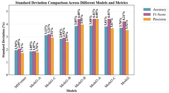
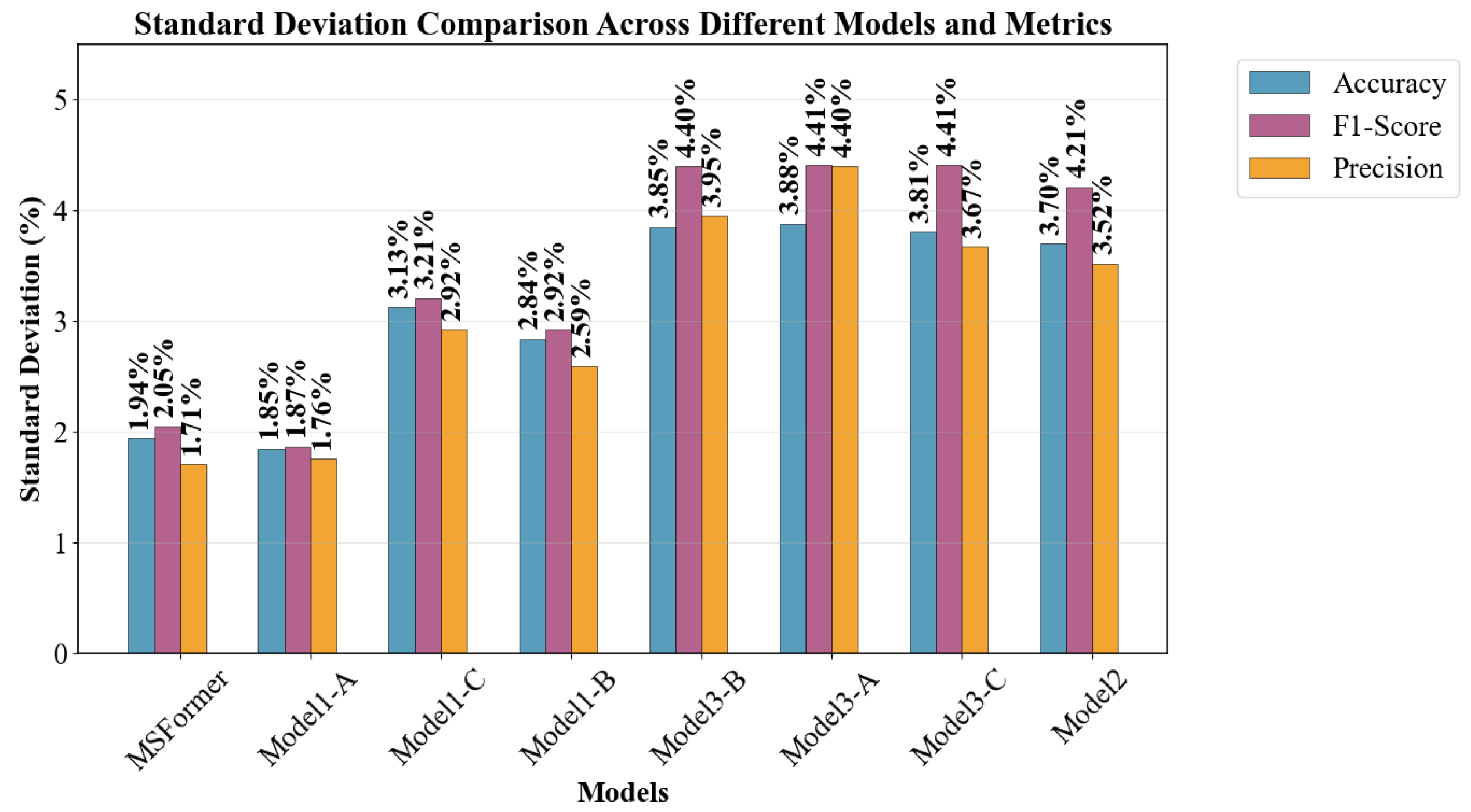
According to the standard deviation comparison across all evaluation metrics in Figure 8, MSFormer consistently demonstrates the highest stability among all models. Its standard deviations in Accuracy, F1-Score, and Precision are the lowest in the entire group, all remaining close to or below approximately 2.0%. This indicates that the performance of MSFormer is minimally influenced by data variation and maintains strong robustness.

Figure 8. Standard deviation comparison of different models across evaluation metrics (Accuracy, F1-Score, and Precision).

In comparison, the remaining models—including Model1-A, Model1-C, Model1-B, Model3-B, Model3-A, Model3-C, and Model2—exhibit noticeably larger fluctuations. For instance, models in the Model3 family show the highest variability, with standard deviations reaching 4.0–4.4% across the metrics, reflecting significant instability. Even relatively better-performing models such as Model1-A and Model1-B still show higher variance than MSFormer, with standard deviations generally ranging from 1.7% to 3.0%.

Taken together, these results show that MSFormer not only surpasses Model1-A but also outperforms all other models in terms of stability. Its substantially lower standard deviations across all metrics confirm that MSFormer provides the most reliable, consistent, and robust predictive behavior among the compared models. This makes MSFormer the most stable and practically deployable model in this study.

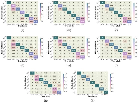
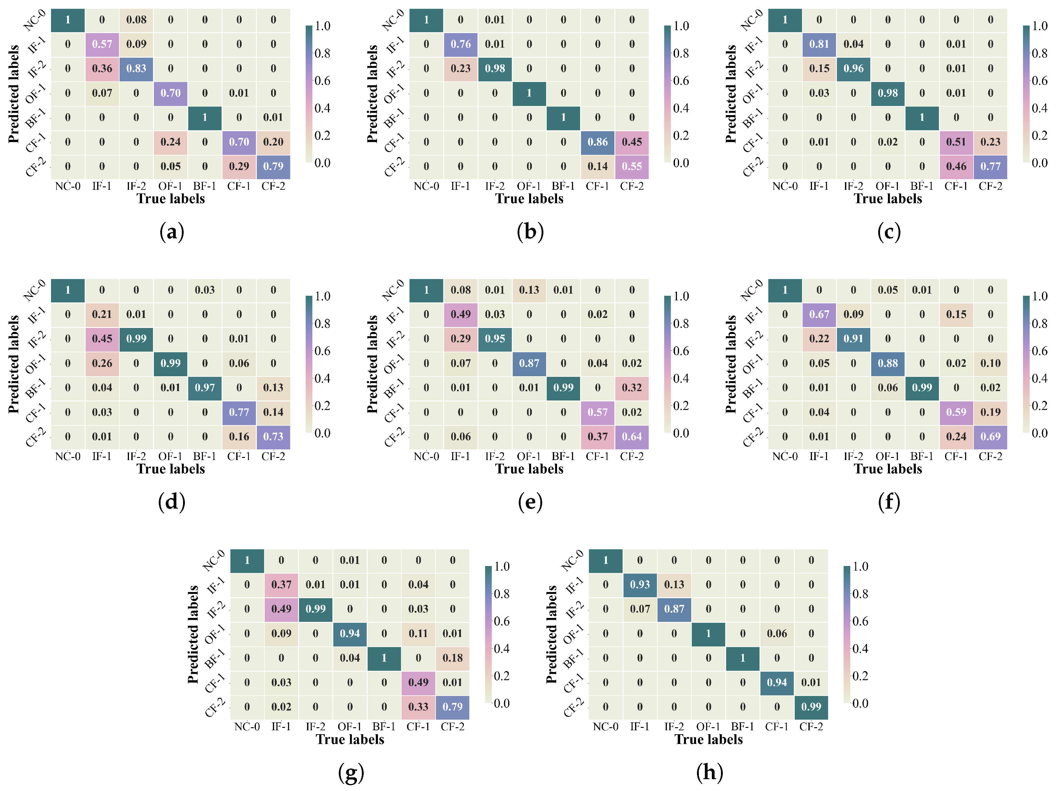
By comparing the confusion matrices in Figure 9, research found that compared with MSFormer, Model 1 shows an extremely high rate of mutual misidentification between CF-2 and CF-1. Additionally, a high rate of misclassification also exists between IF-1 and IF-2. Model 2 tends to misclassify IF-1 as IF-2; CF-1 is also easily confused with CF-2. Model 3 shows a tendency to misclassify IF-1 as IF-2 and CF-1 as CF-2. Moreover, it has low recognition capability for both CF-1 and CF-2. The experimental results demonstrate that MSFormer shows better recognition than the other three models.

Figure 9. Confusion matrices of diagnostic models: (a) Model1-A, (b) Model1-B, (c) Model1-C, (d) Model2, (e) Model3-A, (f) Model3-B, (g) Model3-C, and (h) MSFormer.

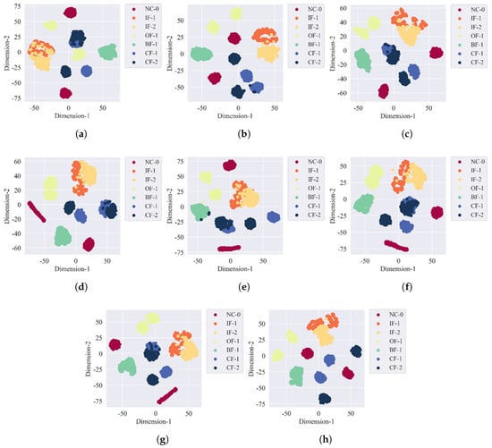
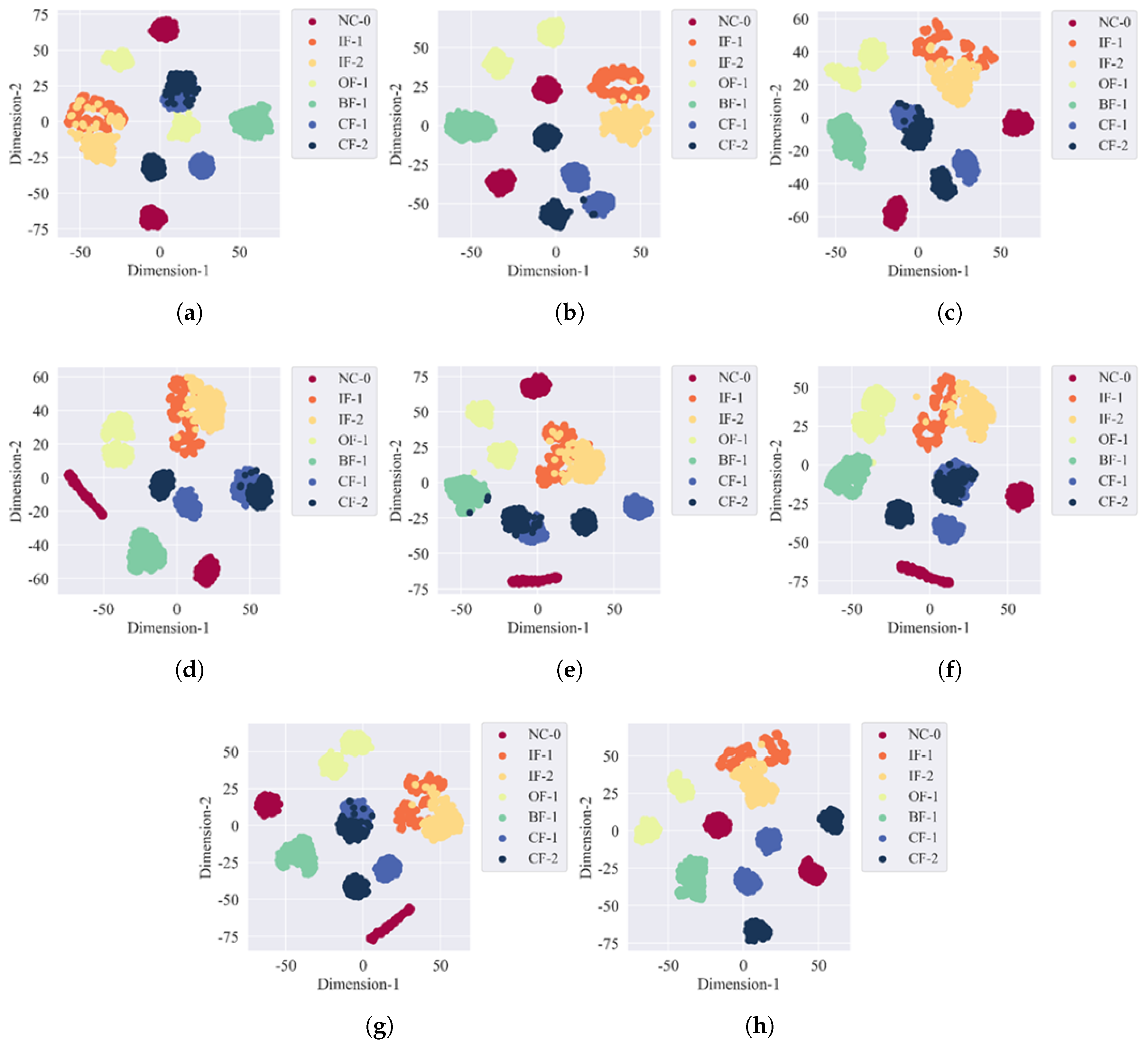
In Figure 10, t-SNE was used to reduce the dimensionality of high-dimensional vibration features to a two-dimensional space. Combined with the visualization results in the document, the analysis is as follows.

Figure 10. The t−SNE feature visualization of diagnostic models: (a) Model1-A, (b) Model1-B, (c) Model1-C, (d) Model2, (e) Model3-A, (f) Model3-B, (g) Model3-C and (h) MSFormer.

• Model 3 (Basic CNN): The feature confusion can be observed. The feature points of CF-1 and CF-2 overlapped. The boundaries between IF-1 and IF-2 are blurred and scattered. This demonstrates that the single-branch CNN can only extract single-scale features, making it unable to distinguish weak local features of incipient faults.
• Model 1 (Single Branch + Transformer): The clustering effect was improved. Clusters of NC-0 and BF-1 were relatively compact, but partial overlap still existed between IF-2 and IF-1. This indicates that although the Transformer module can focus on key features, the single branch fails to cover multi-scale fault features, leading to confusion between similar fault categories.
• Model 2 (Multi-Branch + No Transformer): The inter-class separation was significantly enhanced. The boundaries of clusters for the 7 fault categories were relatively clear, with only slight overlap between CF-2 and CF-1. But partial overlap still existed between IF-2 and IF-1. This confirms that the multi-scale structure can provide rich feature dimensions; however, without the long-range dependency modeling capability of the Transformer module, it still cannot distinguish the subtle differences between cage faults.
• MSFormer: MSFormer generally produces relatively compact clusters with clearer inter-class boundaries. Limited boundary overlap remains between IF-1 and IF-2, but it is less pronounced than in the compared ablation models. Moreover, the other classes are separated except for IF-1 and IF-2 overlapping. This verifies that the synergy of the multi-scale structure and Transformer module can effectively improve the class discriminability of features, providing support for high diagnostic accuracy.

The computational efficiency of the proposed MSFormer was benchmarked against four state-of-the-art diagnostic models. As presented in Table 2, MSFormer achieves a parameter count of 1.37 M, which is highly competitive and compact. While MRCNN shows slightly lower inference latency in specific experimental instances, it lacks the sophisticated feature disentanglement capability of the proposed method. Furthermore, compared to attention-based models such as TCAC and MCSAT, MSFormer demonstrates significantly improved computational efficiency, maintaining real-time inference latency of approximately 52.26 ms/sample. These results confirm that MSFormer strikes an optimal balance between model complexity, computational overhead, and diagnostic precision, establishing its suitability for high-speed, real-time industrial fault diagnosis.

Table 2. Comparison of computational complexity and inference efficiency among different diagnostic models.

Diagnostic Model	Parameters (M)	Inference Latency (ms/Sample)
MCNN	1.38	66.79
MRCNN	1.38	45.78
MCSAT	1.45	85.00
TCAC	1.37	65.75
MSFormer	1.37	52.26

In conclusion, the empirical results demonstrate that the proposed MSFormer exhibits distinctive merits in the diagnosis of mechanical faults under complex operating conditions. Primarily, the multi-scale CNN effectively isolates multi-granular temporal frequency features; specifically, small kernels ($k=4$) lock onto subtle high-frequency transients, while large kernels ($k=16$) integrate structural vibration energy jumps. This, combined with the Transformer encoder’s global long-range dependency modeling, ensures precise fault identification.

The framework maintains an exceptional generalization capacity under restricted data regimes, achieving 92.67% accuracy with only 10 samples per category. This stringent experimental setting is specifically designed as a stress test to the model’s learning efficiency, where the 10-sample constraint serves as a boundary condition to evaluate whether the model can extract invariant fault patterns rather than memorizing training instances. A comparative analysis of model stability reveals that this performance is not an artifact of random overfitting, which refers to the phenomenon where a model captures stochastic noise in the training set rather than the underlying fault patterns. While baseline models, particularly the Transformer-based TCAC, exhibit severe performance collapse that is characterized by an Accuracy standard deviation (SD) reaching 18.52%, MSFormer maintains a remarkably low SD of 1.94%, which provides statistical evidence that the framework successfully strikes an optimal bias–variance trade-off. This statistical discrepancy indicates that while baseline models either suffer from overfitting to the training noise that results in high variance or fail to capture complex signal patterns due to insufficient inductive bias, which is defined here as the set of assumptions that the model uses to predict outputs for inputs it has not encountered, MSFormer leverages its multi-scale convolutions to provide the necessary inductive bias that prevents overfitting. Simultaneously, the hierarchical Transformer encoder ensures sufficient expressive power that avoids underfitting. Furthermore, the confusion matrices reveal that the model significantly reduces misclassification rates among similar fault modes. Qualitative t-SNE visualizations confirm the model’s heightened sensitivity, successfully disentangling the degradation stages that share identical theoretical defect frequencies, where disentanglement is defined as the model’s autonomous capability to isolate distinct physical fault signatures from overlapping transients. This confirms that the model transcends mere frequency counting, instead autonomously learning to resolve subtle physical nuances in the presence of inherent industrial noise (e.g., electromagnetic interference and mechanical misalignment), which demonstrates inherent robustness under low signal-to-noise ratio (SNR) scenarios, where the SNR is defined as a measure that compares the level of a desired signal to the level of background noise. While this study has not performed synthetic noise injection experiments, the consistent performance across the UO dataset indicates robust feature discriminability. Finally, relative to lightweight CNNs, the self-attention mechanisms introduce additional computational overhead, which necessitates a trade-off between diagnostic precision and real-time inference speed.

Finally, while the MSFormer demonstrates robust feature discriminability on the UO dataset under constrained data regimes, it is must be acknowledged that the validation is currently limited to a single domain. Although the statistical consistency observed here suggests high diagnostic reliability rather than overfitting, the true generalization boundaries of this architecture remain to be systematically mapped. Therefore, the multi-source cross-dataset validation should be identified as a primary objective for future research to rigorously establish the model’s performance across varying operating conditions and diverse mechanical configurations. Finally, relative to lightweight CNNs, the self-attention mechanisms introduce additional computational overhead, which necessitates a trade-off between diagnostic precision and real-time inference speed.

5. Conclusions

This paper introduces MSFormer, an innovative end-to-end framework for bearing fault diagnosis that effectively resolves the critical challenges of extreme data scarcity and inherent industrial noise. By synergizing parallel multi-scale convolutional branches with hierarchical Transformer encoders, MSFormer achieves a superior diagnostic accuracy of 92.67% using highly constrained training data. Systematic stability tests confirm the model’s robustness, while visualization results validate its capability to resolve fine-grained fault severity levels that share identical theoretical defect frequencies, which traditional spectral analysis fails to achieve. The significance of this work lies in the transition from manually engineered features to adaptive, data-driven feature extraction, which enables high-fidelity diagnostics under complex physical interferences.

Despite these advancements, the current framework is constrained by a single-label classification paradigm, which limits its ability to disentangle overlapping transient pulses in compound fault scenarios where multiple components fail simultaneously. Furthermore, the reliance on self-attention mechanisms introduces significant computational overhead, posing challenges for real-time inference on edge devices.

Future research will focus on four primary directions: first, extending the framework to handle compound fault separation via multi-label classification to resolve non-linear signal interferences; second, performing rigorous robustness verification under controlled, severe SNR fluctuations using synthetic noise injection; and third, developing model compression techniques to optimize computational complexity, facilitating deployment on resource-constrained industrial hardware. Fourth, generalization ability is critical for the engineering deployment of intelligent diagnostic models. Future work will prioritize improving the generalization of the proposed method under varying operating parameters and different application scenarios.

References

- Neupane, D.; Bouadjenek, M.R.; Dazeley, R.; Aryal, S. Data-driven machinery fault diagnosis: A comprehensive review. Neurocomputing 2025, 627, 129588. [Google Scholar] [CrossRef] [Scilit]
- Lei, Y.; Jia, F.; Lin, J.; Xing, S.; Ding, S. An intelligent fault diagnosis method using unsupervised feature learning towards mechanical big data. IEEE Trans. Ind. Electron. 2016, 63, 3137–3147. [Google Scholar] [CrossRef] [Scilit]
- Jia, F.; Lei, Y.; Lin, J.; Zhou, X.; Lu, N. Deep neural networks: A promising tool for fault characteristic mining and intelligent diagnosis of rotating machinery with massive data. Mech. Syst. Signal Process. 2016, 72, 303–315. [Google Scholar] [CrossRef] [Scilit]
- Chen, G.; Yuan, J.; Zhang, Y.; Zhu, H.; Huang, R.; Wang, F.; Li, W. Enhancing Reliability Through Interpretability: A Comprehensive Survey of Interpretable Intelligent Fault Diagnosis in Rotating Machinery. IEEE Access 2024, 12, 103348–103379. [Google Scholar] [CrossRef] [Scilit]
- Smith, W.A.; Randall, R.B. Rolling element bearing diagnostics using the Case Western Reserve University data: A benchmark study. Mech. Syst. Signal Process. 2015, 64, 100–131. [Google Scholar] [CrossRef] [Scilit]
- Shi, Z.; Chen, J.; Zhang, X.; Zi, Y.; Li, C.; Chen, J. A reliable feature-assisted contrastive generalization net for intelligent fault diagnosis under unseen machines and working conditions. Mech. Syst. Signal Process. 2023, 188, 110003. [Google Scholar] [CrossRef] [Scilit]
- Zhang, T.; Chen, J.; Ye, Z.; Liu, W.; Tang, J. Prior knowledge-informed multi-task dynamic learning for few-shot machinery fault diagnosis. Expert Syst. Appl. 2025, 271, 126439. [Google Scholar] [CrossRef] [Scilit]
- Zhang, T.; Chen, J.; He, S.; Zhou, Z. Prior knowledge-augmented self-supervised feature learning for few-shot intelligent fault diagnosis of machines. IEEE Trans. Ind. Electron. 2022, 69, 10573–10584. [Google Scholar] [CrossRef] [Scilit]
- Li, S.; Liu, J.; Ma, H.; Yang, N. Multimodal Adaptive Signal Fusion for Domain Generalization in Imbalanced Few-Shot Rotating Machinery Fault Diagnosis. IEEE Trans. Instrum. Meas. 2025, 74, 3568716. [Google Scholar] [CrossRef] [Scilit]
- Lu, Z.; Liang, L.; Zhu, J.; Zou, W.; Mao, L. Rotating Machinery Fault Diagnosis Under Multiple Working Conditions via a Time-Series Transformer Enhanced by Convolutional Neural Network. IEEE Trans. Instrum. Meas. 2023, 72, 3533611. [Google Scholar] [CrossRef] [Scilit]
- Shen, H.; Tang, X.; Luo, Y.; Xie, F.; Shi, Z. Online Open-Circuit Fault Diagnosis for Neutral Point Clamped Inverter Based on an Improved Convolutional Neural Network and Sample Amplification Method Under Varying Operating Conditions. IEEE Trans. Instrum. Meas. 2024, 73, 3512612. [Google Scholar] [CrossRef] [Scilit]
- Zhang, Y.; Ding, J.; Li, Y.; Ren, Z.; Feng, K. Multi-modal data cross-domain fusion network for gearbox fault diagnosis under variable operating conditions. Eng. Appl. Artif. Intell. 2024, 133, 108236. [Google Scholar] [CrossRef] [Scilit]
- Zhu, X.; Zhao, X.; Yao, J.; Deng, W.; Shao, H.; Liu, Z. Adaptive Multiscale Convolution Manifold Embedding Networks for Intelligent Fault Diagnosis of Servo Motor-Cylindrical Rolling Bearing Under Variable Working Conditions. IEEE/ASME Trans. Mechatron. 2024, 29, 2230–2240. [Google Scholar] [CrossRef] [Scilit]
- Zhao, X.; Yao, J.; Deng, W.; Ding, P.; Zhuang, J.; Liu, Z. Multiscale Deep Graph Convolutional Networks for Intelligent Fault Diagnosis of Rotor-Bearing System Under Fluctuating Working Conditions. IEEE Trans. Ind. Inform. 2023, 19, 166–176. [Google Scholar] [CrossRef] [Scilit]
- Liu, Z.; Peng, Z. Few-shot bearing fault diagnosis by semi-supervised meta-learning with graph convolutional neural network under variable working conditions. Measurement 2025, 240, 115402. [Google Scholar] [CrossRef] [Scilit]
- Song, B.; Liu, Y.; Fang, J.; Liu, W.; Zhong, M.; Liu, X. An optimized CNN-BiLSTM network for bearing fault diagnosis under multiple working conditions with limited training samples. Neurocomputing 2024, 574, 127284. [Google Scholar] [CrossRef] [Scilit]
- Wang, X.; Mao, D.; Li, X. Bearing fault diagnosis based on vibro-acoustic data fusion and 1D-CNN network. Measurement 2021, 173, 108518. [Google Scholar] [CrossRef] [Scilit]
- Chang, X.; Lyu, J.; Ma, H. Motor Bearing Fault Diagnosis Based on EMD-CNN-Transformer. In The Proceedings of the 20th Annual Conference of China Electrotechnical Society; Lecture Notes in Electrical Engineering; Springer: Singapore, 2026; Volume 1559. [Google Scholar] [CrossRef] [Scilit]
- Zhang, Y.; Zhou, T.; Huang, X.; Cao, L.; Zhou, Q. Fault diagnosis of rotating machinery based on recurrent neural networks. Measurement 2021, 171, 108774. [Google Scholar] [CrossRef] [Scilit]
- Vaswani, A.; Shazeer, N.; Parmar, N.; Uszkoreit, J.; Jones, L.; Gomez, A.N.; Kaiser, L.; Polosukhin, I. Attention is all you need. In Proceedings of the 31st International Conference on Neural Information Processing Systems (NIPS 2017), Long Beach, CA, USA, 4–9 December 2017; Curran Associates Inc.: Red Hook, NY, USA, 2017; pp. 6000–6010. [Google Scholar]
- Dosovitskiy, A.; Beyer, L.; Kolesnikov, A.; Weissenborn, D.; Zhai, X.; Unterthiner, T.; Dehghani, M.; Minderer, M.; Heigold, G.; Gelly, S.; et al. An image is worth 16 × 16 words: Transformers for image recognition at scale. In Proceedings of the International Conference on Learning Representations (ICLR), Vienna, Austria, 4 May 2021. [Google Scholar]
- Zhou, H.; Zhang, S.; Peng, J.; Zhang, S.; Li, J.; Xiong, H.; Zhang, W. Informer: Beyond Efficient Transformer for Long Sequence Time-Series Forecasting. In Proceedings of the AAAI Conference on Artificial Intelligence, Virtual Conference, 2–9 February 2021; Volume 35, pp. 11106–11115. [Google Scholar] [CrossRef] [Scilit]
- Ding, Y.; Jia, M.; Miao, Q.; Cao, Y. A novel time–frequency Transformer based on self–attention mechanism and its application in fault diagnosis of rolling bearings. Mech. Syst. Signal Process. 2022, 168, 108616. [Google Scholar] [CrossRef] [Scilit]
- An, Y.; Zhang, K.; Chai, Y.; Zhu, Z.; Liu, Q. Gaussian Mixture Variational-Based Transformer Domain Adaptation Fault Diagnosis Method and Its Application in Bearing Fault Diagnosis. IEEE Trans. Ind. Inform. 2024, 20, 615–625. [Google Scholar] [CrossRef] [Scilit]
- Li, S.; Yu, J. A Multisource Domain Adaptation Network for Process Fault Diagnosis Under Different Working Conditions. IEEE Trans. Ind. Electron. 2023, 70, 6272–6283. [Google Scholar] [CrossRef] [Scilit]
- Zhao, C.; Shen, W. Mutual-assistance semisupervised domain generalization network for intelligent fault diagnosis under unseen working conditions. Mech. Syst. Signal Process. 2023, 189, 110074. [Google Scholar] [CrossRef] [Scilit]
- Yang, X.; Yuan, X.; Ye, T.; Zhu, W.; Zhou, F.; Jin, J. PSNN-TADA: Prototype and Stochastic Neural Network-Based Twice Adversarial Domain Adaptation for Fault Diagnosis Under Varying Working Conditions. IEEE Trans. Instrum. Meas. 2024, 73, 3500212. [Google Scholar] [CrossRef] [Scilit]
- An, Z.; Jiang, X.; Liu, J. Mode-Decoupling Auto-Encoder for Machinery Fault Diagnosis Under Unknown Working Conditions. IEEE Trans. Ind. Inform. 2024, 20, 4990–5003. [Google Scholar] [CrossRef] [Scilit]
- Chen, X.; Zhang, B.; Gao, D. Bearing fault diagnosis base on multi-scale CNN and LSTM model. J. Intell. Manuf. 2021, 32, 971–987. [Google Scholar] [CrossRef] [Scilit]
- Sehri, M.; Dumond, P.; Bouchard, M. University of Ottawa constant load and speed rolling-element bearing vibration and acoustic fault signature datasets. Data Brief 2023, 49, 109327. [Google Scholar] [CrossRef] [Scilit] [PubMed]
- Xia, Y.; Zhang, D.; Liu, C.; Cao, Z.; Su, Y.; Chen, Y. Fault diagnosis of air handling units based on an MCNN-Transformer ensemble learning. J. Process Control 2025, 154, 103526. [Google Scholar] [CrossRef] [Scilit]
- Zhuang, X.; Ge, J.; Mao, X.; Zhou, D.; Yao, H.; Sun, W.; Li, L.; Xiang, J. A novel lightweight model combined with convolutional neural network and transformer for gearbox fault diagnosis using infrared thermal images. Eng. Appl. Artif. Intell. 2025, 162, 112704. [Google Scholar] [CrossRef] [Scilit]
- Yao, Z.; Jiang, Q.; Gu, X. A fusion model fault diagnosis scheme based on multibranch multiscale residual convolutional network with Transformer. Chem. Eng. Res. Des. 2025, 220, 667–681. [Google Scholar] [CrossRef] [Scilit]
- Zhang, J.; Zhang, M.; Wang, D.; Yang, M.; Liang, C. Multi-scale convolutional sparse attention transformer: A lightweight fault diagnosis model for rotating machinery. Neurocomputing 2025, 650, 130934. [Google Scholar] [CrossRef] [Scilit]
Disclaimer/Publisher’s Note: The statements, opinions and data contained in all publications are solely those of the individual author(s) and contributor(s) and not of MDPI and/or the editor(s). MDPI and/or the editor(s) disclaim responsibility for any injury to people or property resulting from any ideas, methods, instructions or products referred to in the content. |
© 2026 by the authors. Licensee MDPI, Basel, Switzerland. This article is an open access article distributed under the terms and conditions of the Creative Commons Attribution (CC BY) license.