


Abstract
Shallow defects in ferromagnetic components may produce weak and unstable magnetic flux leakage responses in compact inspection devices, whereas an inductive response alone does not provide the same depth-related magnetic information. To obtain complementary defect information, this study proposes a magnetic–inductive dual-channel inspection method that integrates an MLX90393 three-axis digital magnetic sensor with a PCB planar spiral coil and an LDC1612 inductance-to-digital converter. Because the two sensing units are physically separated on the detection board, peak-position offset analysis and spatial registration were introduced to associate their responses to the same defect region. Controlled experiments were conducted on a laboratory pipeline inspection platform using a Q235 defect specimen installed at the internal inspection position of the pipe. The defects were machined on the inner surface, which was also the inspection surface. For each defect, five motor-driven axial scans were performed at 10 mm/s, with 400 samples acquired at 100 Hz during each 4 s scan. Response amplitude, signal-to-noise ratio, peak position, and repeatability were evaluated. For the square-hole defects, the magnetic response amplitude decreased from 675.0 to 98.5 a.u. as the depth ratio decreased from 50% to 10%, while the magnetic-channel SNR decreased from 30.5 to 4.7. For the 10% depth defect, the inductive channel retained an average SNR of 434.4 and a coefficient of variation of 0.23%, providing a stable auxiliary response. However, the pre-registration peak-position offset measured for this shallow defect was sampling points, indicating substantial uncertainty in using a single magnetic extremum for scan-specific registration when the magnetic response was weak. These results demonstrate that the two channels provide different and complementary information under controlled laboratory conditions, while further validation is required for irregular corrosion, other ferromagnetic components, and practical inspection conditions.
1. Introduction
Ferromagnetic components are widely used in industrial systems, with pipelines representing an important application scenario because of their high transport capacity, continuous operation, and relatively low operating cost. During long-term service, pipelines and other ferromagnetic components may be affected by corrosion, external loading, stress concentration, material aging, and local mechanical damage. These factors may cause wall thinning, pits, cracks, holes, and other local defects. If such defects are not detected or characterized in time, they may further develop into leakage, structural failure, environmental pollution, or serious safety accidents. Therefore, reliable nondestructive inspection and defect characterization methods are important for the safety assessment and maintenance of ferromagnetic engineering components [1].
Magnetic flux leakage (MFL) testing is widely used for the nondestructive inspection of ferromagnetic components, particularly pipelines. In MFL testing, the pipe wall is magnetized by an external magnetic field, and local defects disturb the magnetic permeability and magnetic reluctance distribution around the defect region [2]. This disturbance causes part of the magnetic flux to leak out of the material surface, and the leakage magnetic field can be measured by magnetic sensors. Pipeline in-line inspection systems based on MFL have been widely studied in terms of sensing structures, inspection platforms, instrumentation, and data management [3]. Recent reviews have summarized the development of MFL nondestructive testing from sensing principles, defect modeling, and signal interpretation perspectives [4]. Data-driven methods have also been introduced to improve MFL signal interpretation for pipeline defect detection and evaluation [5]. Analytical and numerical MFL models have been used to describe the spatial magnetic field distribution caused by surface-breaking defects [6]. Compared with single-axis sensing, three-axis magnetic sensing can provide more complete information about the spatial distribution of leakage magnetic fields and improve defect characterization capability [7].
Nevertheless, in compact inspection systems for ferromagnetic components, the installation space, sensor size, and available detection channels are often limited. The magnetic response is affected by magnetization condition, lift-off height, scanning speed, sensor posture, defect geometry, and local surface disturbance. Lift-off-related variation may change the measured leakage magnetic field and reduce the stability of defect characterization [8]. Operating speed and motion-related effects may also influence the amplitude and shape of MFL signals during scanning [9]. Under shallow-defect conditions, the leakage magnetic field may decrease significantly, resulting in weak response amplitude, reduced signal-to-noise ratio, and unstable peak position. Therefore, relying only on a single magnetic sensing channel may be insufficient for stable shallow-defect characterization in compact inspection devices.
In addition to MFL testing, eddy current testing is widely used for nondestructive evaluation of conductive or ferromagnetic materials [10]. Pulsed eddy current testing can provide electromagnetic response information related to near-surface and subsurface discontinuities [11]. Magnetic-field-based and eddy-current-based sensor structures have also been investigated for nondestructive testing applications [12]. Eddy current probe design is closely related to coil geometry, excitation mode, lift-off condition, and defect sensitivity [13]. Magnetoresistive and differential measurement structures have been used to improve the sensitivity of eddy current probes [14]. Flexible eddy current array sensors have been developed for surface micro-defect inspection on complex or curved surfaces [15]. Resolution-enhanced eddy current array probes have been proposed to improve the spatial resolution for small-defect inspection [16]. The curvature of metal components can affect the amplitude and consistency of flexible eddy current array signals [17]. Multifrequency inductive sensing has been used to reduce lift-off-related influence in electromagnetic property measurements [18]. PCB-based planar inductive loops have been reported as compact electromagnetic sensing structures because of their small size and ease of integration [19]. Planar spiral coils have also been investigated for inductive sensing applications where compact coil geometry and sensitivity are important [20]. Quantitative electromagnetic feature extraction has been investigated for surface crack characterization, indicating the importance of reliable signal features in eddy-current-based inspection [21]. Classical analytical solutions for probe-coil problems provide theoretical support for understanding electromagnetic coupling between coils and conductive specimens [22]. Frequency-domain analysis of MFL signals in ferromagnetic pipe inspection also shows that complementary signal features can be useful for defect characterization [23]. Therefore, an inductive sensing channel may provide complementary information to the magnetic channel, especially when the magnetic response becomes weak for shallow defects.
Although magnetic flux leakage and inductive inspection methods have each been widely investigated, their sensing mechanisms and the information contained in their responses are different. The magnetic channel measures the leakage magnetic field produced by changes in the magnetic-reluctance distribution around a defect. Its response therefore provides magnetic information related to defect geometry and, under otherwise comparable conditions, exhibits a clear variation with defect depth. By contrast, the inductive channel measures changes in the electromagnetic coupling between the PCB coil and the conductive ferromagnetic surface. Its response is influenced by local material continuity, geometry, permeability, conductivity, and lift-off. Consequently, the inductive response should not be regarded as a replacement for the magnetic response, even when it exhibits a numerically higher SNR.
For compact inspection devices used with ferromagnetic components, integrating these two sensing mechanisms presents two practical challenges. First, the magnetic sensor and the PCB coil have different output scales and noise characteristics; therefore, their amplitudes and SNR values cannot be interpreted through direct numerical ranking. Second, the two sensing units are physically separated on the detection board. Their responses to the same defect consequently appear at different sampling positions before registration. Directly combining the two signals without compensating for this position difference may associate magnetic and inductive features obtained from different physical locations.
The purpose of the proposed dual-channel method is therefore not to demonstrate that the inductive channel is superior to the magnetic channel. Instead, it is to construct a spatially corresponding description in which the magnetic channel provides a depth-dependent leakage-field response, while the inductive channel supplies a stable auxiliary response when the magnetic signal becomes weak. The two types of information are complementary: the high SNR of the inductive channel does not independently establish defect-depth characterization, and the magnetic channel alone becomes less stable for the shallowest defect considered in this study.
To investigate this complementary relationship, a compact magnetic–inductive dual-channel inspection board was developed by integrating an MLX90393 three-axis magnetic sensor with a PCB planar spiral coil and an LDC1612 inductance-to-digital converter. Because the two sensing units were spatially separated along the scanning direction, their pre-registration peak-position differences were measured for each repeated scan and used as scan-specific offsets for spatial alignment. The validation experiments were conducted on a laboratory pipeline inspection platform, in which the Q235 defect specimens were installed at the internal inspection position and the motor-driven detection board scanned axially along the inner pipe surface. The contribution of this study lies not in introducing either magnetic flux leakage or inductive sensing individually, but in integrating the two sensing mechanisms within a compact inspection board, establishing their spatial correspondence, and quantitatively evaluating their complementary responses under shallow-defect conditions. The present experiments were designed as a controlled laboratory validation of this sensing and registration strategy. They do not constitute comprehensive validation under in-service field conditions involving irregular corrosion, coatings, lift-off fluctuations, scanning-speed variations, vibration, or complex pipe curvature.
The main contributions of this study are summarized as follows:
- (1)
- A compact magnetic–inductive dual-channel sensing structure was developed by integrating a three-axis magnetic sensor and a PCB planar spiral coil on the same detection board. The integrated structure acquires leakage-magnetic-field information and inductive coupling information from the same defect region using two different sensing mechanisms.
- (2)
- A scan-specific spatial registration procedure was established for the physically separated sensing units. The magnetic and inductive peak positions were extracted before registration, and their measured difference was used to align the two response regions to a common sampling reference. This procedure provides a position-corresponding basis for dual-channel comparison, while its uncertainty under weak magnetic-response conditions is explicitly evaluated.
- (3)
- The complementary roles of the two channels were quantitatively evaluated using response amplitude, SNR, peak position, and repeatability obtained from five repeated scans of four defects. The magnetic response exhibited a pronounced depth-dependent trend for the square-hole defects, whereas the inductive channel maintained stable repeatability and a high SNR for the shallowest defect. The results are interpreted as complementary sensing characteristics rather than evidence of the absolute superiority of either channel.
The remainder of this paper is organized as follows. Section 2 describes the materials, dual-channel sensing principle, experimental setup, data acquisition, spatial registration, and feature extraction method. Section 3 presents the experimental results. Section 4 discusses the complementary sensing capability, spatial registration necessity, implications, and limitations of the proposed method. Section 5 concludes the paper.
2. Materials and Methods
2.1. Dual-Channel Inspection Principle
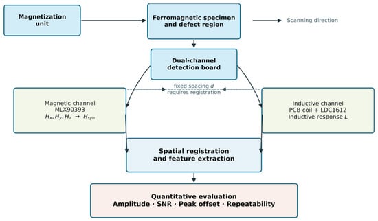
The proposed inspection method is based on the complementary response characteristics of a magnetic flux leakage sensing channel and an inductive sensing channel. The magnetic channel is mainly used to measure the leakage magnetic field caused by local magnetic reluctance changes around defects in ferromagnetic materials. The inductive channel is used to measure the variation in electromagnetic coupling between a PCB planar spiral coil and the metallic specimen surface. By integrating the two sensing units on the same compact detection board, the defect region can be characterized from two different electromagnetic perspectives.
During scanning, the detection board moves along the surface of the Q235 steel specimen. When the board passes over a defect region, the local discontinuity changes the magnetic field distribution and the electromagnetic coupling condition. As a result, both the three-axis magnetic sensor and the inductive sensing unit produce local response variations. Since the two sensing units are not located at the same physical position on the detection board, their response peaks do not appear at the same sampling point. Therefore, spatial registration is required before dual-channel feature construction.
The overall workflow of the proposed magnetic-inductive dual-channel inspection method is shown in Figure 1.
Figure 1.
Schematic diagram of the magnetic–inductive dual-channel inspection method. The arrows indicate the scanning direction and processing flow, while the colors distinguish the functional modules.
2.2. Magnetic Flux Leakage Sensing Channel
A three-axis digital magnetic sensor was used as the main magnetic flux leakage sensing channel. The sensor measures the magnetic field components along three orthogonal directions during scanning. At the scanning position (x), the three-axis magnetic field vector can be expressed as
where , , and denote the magnetic field components along the scanning direction, transverse direction, and normal direction, respectively. To reduce the dependence on a single sensitive direction and to describe the overall magnetic disturbance intensity, the resultant magnetic response is defined as
Compared with a single-axis magnetic signal, the resultant magnetic response provides a more comprehensive representation of the local leakage magnetic field around the defect. In this study, was used as the main magnetic feature signal for subsequent amplitude, signal-to-noise ratio, peak position, and repeatability analysis.
2.3. Inductive Auxiliary Sensing Channel
The inductive auxiliary channel consists of a PCB planar spiral coil, a resonant capacitor, and an inductance-to-digital converter. The PCB coil and the capacitor form an LC resonant circuit. Its resonant frequency can be expressed as
where is the equivalent inductance of the coil and is the resonant capacitance. When the coil approaches a metallic specimen, the electromagnetic coupling between the coil and the specimen is affected by the material conductivity, magnetic permeability, lift-off height, and local geometry. When the coil passes over a defect region, the local discontinuity changes the equivalent electromagnetic coupling condition, resulting in a measurable variation in the digital output of the inductive channel.
In this study, the original digital output of the inductance-to-digital converter was directly used as the inductive response signal. This avoids additional uncertainty introduced by converting the digital output into equivalent inductance or resonant frequency. The inductive response at the -th sampling point is denoted as .
2.4. Experimental System and Defect Specimens
The experiments were conducted using a laboratory pipeline inspection platform rather than an isolated flat-plate test bench. The experimental system consisted of a pipe platform, a Q235 defect specimen installed at the internal inspection position, a custom-built magnetization unit, a custom-built motor-driven scanning mechanism, a dual-channel detection board, a custom-developed data acquisition and storage module, and a custom-developed offline signal-processing program implemented in Python 3.11. The defects were located on the inner surface, which was also the inspection surface.
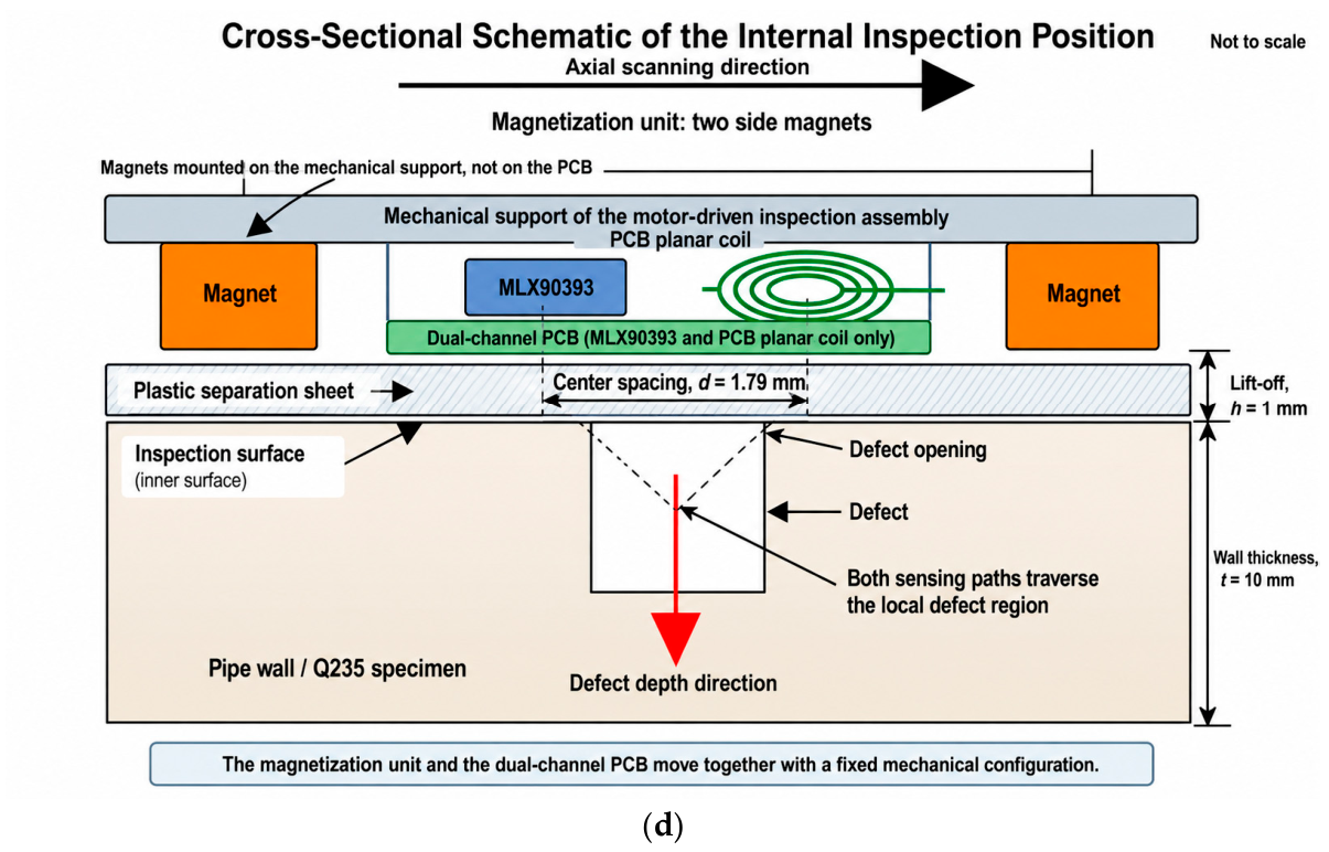
During each scan, the detection board was driven by a motor along the axial direction of the pipe, from one end of the inspection section toward the other. The scanning speed was 10 mm/s. The sensing components were maintained close to the inner pipe wall through a 1 mm thick plastic separation sheet, resulting in a 1 mm lift-off between the sensing assembly and the inspection surface.
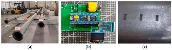
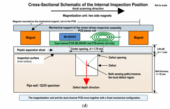
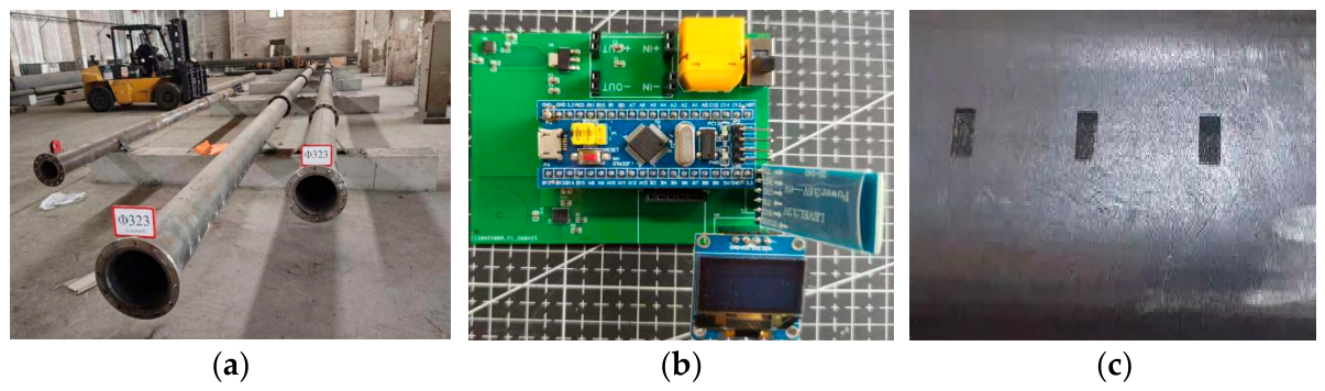
Figure 2a shows the laboratory pipeline inspection platform used in the controlled experiments. The Q235 defect specimen shown in Figure 2c was installed at the internal inspection position of the pipe rather than tested as an isolated external plate. The defect openings were located on the inner surface, which was also the inspection surface. During each scan, the motor-driven detection board shown in Figure 2b moved axially along the inner pipe surface from one end of the inspection section toward the other. As illustrated in Figure 2d, the defect depth extended from the inner-surface opening toward the wall-thickness direction. The MLX90393 and PCB planar coil were positioned on the same side as the defect openings through a 1 mm plastic separation sheet. Their measurement paths both traversed the local defect region, while their center-to-center separation along the scanning direction was 1.79 mm.
Figure 2.
Experimental configuration of the laboratory pipeline inspection platform: (a) laboratory pipeline inspection platform; (b) magnetic–inductive dual-channel detection board; (c) Q235 defect specimen; and (d) schematic cross-sectional relationship among the inner pipe wall, defect, magnetization unit, MLX90393, PCB planar coil, plastic separation sheet, lift-off, and scanning direction. The black arrows indicate the scanning direction and component annotations, the red arrow indicates the defect-depth direction, and the colors are used to distinguish the sensing and magnetization components.
The magnetization assembly contained two magnets positioned on the two sides of the sensing assembly. Each magnet had planar dimensions of 20 mm × 20 mm. The magnets provided the external magnetic field required for magnetic flux leakage measurement during scanning.
The magnetization unit was mechanically mounted on the motor-driven inspection assembly and moved together with the sensing board during scanning; the magnets were not mounted directly on the PCB. The PCB carried the MLX90393ELW-ABA-014-SP, the planar spiral coil, and the associated electronic components. This mechanical arrangement allowed the magnetization unit and the dual-channel sensing board to maintain a fixed relative configuration during each controlled scan.
The magnetic sensing channel used an MLX90393ELW-ABA-014-SP three-axis digital magnetic sensor (Melexis Technologies NV, Tessenderlo-Ham, Belgium). The inductive sensing channel consisted of a PCB planar spiral coil connected to the IN0 channel of an LDC1612DNTR inductance-to-digital converter (Texas Instruments Incorporated, Dallas, TX, USA). The PCB coil had an outer diameter of 270 mil (6.858 mm), an inner diameter of 50 mil (1.270 mm), 20 turns, and a track width/spacing of 6 mil/6 mil (0.1524 mm/0.1524 mm). The resonant capacitor was 100 pF, and the LDC1612 IDRIVE setting code was 19.The preliminary LDC1612 IDRIVE parameter-test results are provided in the Supplementary Materials.
The center-to-center distance between the MLX90393 and the PCB coil along the scanning direction was 1.79 mm. At a scanning speed of 10 mm/s and a sampling frequency of 100 Hz, this distance corresponded to 17.9 sampling intervals. During scanning, the trajectories of both sensing units traversed the defect opening and central region, thereby acquiring their respective local responses at different sampling positions before spatial registration. The geometric and operating parameters of the inspection system are summarized in Table 1.
Table 1.
Geometric and operating parameters of the dual-channel inspection system.
The defect specimen was made of Q235 steel with a thickness of 10 mm. Four machined defects were investigated: a 50% depth square-hole defect, a 30% depth square-hole defect, a 10% depth square-hole defect, and a 30% depth circular-hole defect. All defect openings were located on the inner surface, which was also the inspection surface, and the defect depths extended from the inner-surface openings toward the wall-thickness direction. The spacing between adjacent defects was sufficiently large to prevent overlap between neighboring defect-response regions. During scanning, the PCB coil trajectory traversed each defect opening and sequentially sampled its local inductive response, while the MLX90393 measurement path passed through the central defect region and acquired the corresponding local magnetic-flux-leakage response. The confirmed defect parameters and test conditions are summarized in Table 2. For each defect, five repeated scans were conducted, with 400 sampling points acquired in each scan.
Table 2.
Geometry, surface location, and test conditions of the tested defects.
2.5. Data Acquisition and Signal Preprocessing
The two sensing channels were sampled under the same acquisition sequence. The sampling frequency was 100 Hz, and each scan contained 400 sampling points, corresponding to a scanning duration of 4 s. Under constant-speed scanning, the spatial sampling interval was jointly determined by the scanning speed and sampling frequency:
where is the scanning speed, is the sampling frequency, and is the spatial distance between two consecutive sampling positions. Therefore, the acquisition system provided one sampling position per 0.1 mm of probe travel. During the 4 s acquisition period, the motor-driven scanning mechanism traveled a nominal distance of 40 mm.
The relationship in Equation (4) also provides a basis for adapting the acquisition parameters to different scanning speeds. If the scanning speed is increased, the sampling frequency should be increased proportionally to maintain the required spatial sampling interval. Therefore, the present scanning speed of 10 mm/s represents the controlled operating condition used in this study rather than an inherent limitation of the spatial-sampling principle. In practical applications, the scanning speed and sampling frequency should be jointly selected according to the target defect dimensions and required spatial resolution. The achievable parameter range is also constrained by the output data rate of the magnetic sensor, the conversion bandwidth of the inductive channel, data-transmission and storage capacity, and the motion stability of the inspection platform. Consequently, implementation at higher scanning speeds requires corresponding hardware configuration and experimental calibration rather than a direct extrapolation of the present operating parameters.
The relationship between the defect length along the scanning direction and the corresponding number of sampling intervals can be expressed as
where denotes the defect dimension projected along the scanning direction and is the corresponding number of spatial sampling intervals. For D1–D3, the dimension along the scanning direction was the 20 mm side length of the square opening. For D4, the corresponding dimension was its 20 mm diameter. Therefore, all four test defects corresponded to 200 sampling intervals along the scanning direction. The total scanning travel was 40 mm, providing signal regions before and after the 20 mm defect opening for baseline and defect-response evaluation.
The PCB coil had an outer diameter of 6.858 mm, corresponding geometrically to 68.58 spatial sampling intervals along the scanning coordinate. This comparison characterizes the sampling density relative to the probe geometry and should not be interpreted as the intrinsic spatial resolution of the inductive channel. During scanning, the trajectories of both sensing units traversed the opening and central region of each defect. The PCB coil sequentially sampled the local inductive response as it moved across the defect opening, while the MLX90393 measurement path passed through the central defect region and acquired the corresponding local magnetic-flux-leakage response. Thus, the stated probe coverage refers to coverage achieved along the scanning trajectory rather than instantaneous coverage of the entire 20 mm defect opening by the 6.858 mm PCB coil. Both channels acquired multiple consecutive samples over the local defect-response region. Under the present controlled scanning conditions, the 0.1 mm spatial sampling interval was sufficient to describe the measured response curves and to extract amplitude, SNR, and peak-position features. This statement applies only to the present defect experiments and does not imply equivalent performance for arbitrary defect dimensions or field inspection conditions.
The dual-channel data frame at the -th sampling point is defined as
where is the sampling index, is the sampling time, , , and are the three-axis magnetic field components, and is the inductive channel output.
To ensure consistent and reproducible feature extraction, a baseline window and a defect-response window were defined for each scan. The baseline window was selected from stable signal regions sufficiently far from the defect-response region, where no evident defect-related variation was present. The defect-response window was defined around the known defect position and encompassed the local response produced as the sensing trajectory traversed the defect opening. The same window-selection principle was applied to both sensing channels, all four defects, and all five repeated scans. The windows were not independently adjusted to maximize the response amplitude or of an individual scan.
Because the magnetic sensor and the PCB coil were physically separated, their response regions appeared at different sampling positions before registration. Accordingly, the same spatial window-selection principle was applied in the respective sampling coordinates of the two channels before registration. When the registered dual-channel responses were compared, the inductive response window was shifted using the measured pre-registration offset described in Section 2.6.
For a generic raw signal , representing either the resultant magnetic response or the inductive response, let denote the number of samples in the baseline window . The mean baseline level was calculated from the samples in , and the baseline-corrected signal was obtained as follows:
Let denote the defect-response window. The response amplitude A was defined as the maximum absolute value of the baseline-corrected signal within :
The baseline-noise level was calculated as the sample standard deviation of the raw signal within the baseline window :
The signal-to-noise ratio was calculated as the ratio of the response amplitude A to the baseline-noise standard deviation :
The reported is therefore a dimensionless linear amplitude ratio rather than a value expressed in decibels. The same definitions of A, , and were applied to the resultant magnetic response and the inductive response. This unified procedure ensured that the amplitude, baseline noise, and were calculated according to the same window-selection principle for D1–D4 and all repeated scans.
The coefficient of variation was calculated from the response amplitudes obtained from the five repeated scans as
where and denote the mean and standard deviation of the five response amplitudes, respectively. The CV was calculated separately for the magnetic and inductive channels to evaluate their repeated-scan dispersion.
2.6. Spatial Registration and Feature Extraction
The MLX90393 and the PCB planar coil were physically separated along the scanning direction, with a confirmed center-to-center distance of . This fixed hardware separation provided a nominal geometric reference for registration. If is the sensor-to-coil center distance, is the scanning speed, and is the sampling frequency, the nominal geometric time offset is
The corresponding nominal geometric offset in sampling intervals is
Thus, the confirmed hardware separation corresponded to a nominal time offset of and a nominal spatial offset of 17.9 sampling intervals. These values represent the theoretical offset calculated from the sensor geometry and operating parameters. They should not be interpreted as the measured difference between the two response extrema or as the residual positioning error after registration. The measured values presented later in Section 3.4 are pre-registration, scan-specific peak-position offsets used to perform the alignment.
Because the extrema of the magnetic and inductive response curves do not necessarily occur exactly when the respective sensing-unit centers pass over the defect center, the measured peak-position offset may differ from the nominal geometric offset. For each repeated scan , the pre-registration peak position of each channel was defined as the sampling index corresponding to the maximum absolute value of the baseline-corrected response within the predefined defect-response window. The scan-specific peak-position offset was then calculated as
where and are the pre-registration peak positions of the inductive response and resultant magnetic response, respectively, in the -th repeated scan. A positive value of indicates that the inductive peak occurs later than the magnetic peak along the present scanning direction. The corresponding statistical results are presented in Section 3.4.
Under the present scanning direction, the inductive response occurred later than the magnetic response. The inductive signal was therefore shifted toward lower sampling indices using the measured scan-specific offset:
where is the original inductive response and is the registered inductive response for the -th scan. This operation associates the magnetic and inductive response regions with a common sampling reference under the present controlled scanning conditions. Because the method relies on the extracted magnetic extremum, the registration uncertainty increases when the magnetic response becomes weak, as observed for D3. Therefore, the present procedure should be interpreted as scan-specific response alignment rather than complete elimination of shallow-defect localization uncertainty.
For each repeated scan, the following dual-channel feature vector was constructed:
where , , and are the response amplitude, signal-to-noise ratio, and pre-registration peak position of the resultant magnetic response, respectively. Similarly, , , and are the corresponding inductive-response features, and is the measured pre-registration peak-position offset. These features were used to evaluate response strength, noise robustness, position consistency, and repeatability. The registered inductive response was used when the spatially corresponding dual-channel response regions were compared.
3. Results
3.1. Dual-Channel Response Curves
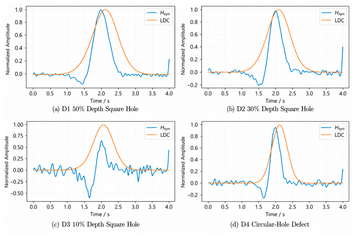
Figure 3 shows the average dual-channel response curves of the four defects after baseline correction. For each defect, five repeated scans were processed, and the mean response curves of the resultant magnetic signal and the inductive signal were obtained. The resultant magnetic response and the inductive response both exhibit local variations when the detection board passes over the defect region, indicating that the two sensing channels can respond to the electromagnetic disturbance caused by defects.
Figure 3.
Average dual-channel response curves of the four defects: (a) D1, 50% depth square-hole defect; (b) D2, 30% depth square-hole defect; (c) D3, 10% depth square-hole defect; and (d) D4, 30% depth circular-hole defect.
For the square-hole defects D1–D3, the resultant magnetic response exhibited a pronounced depth-related trend. D1, with a depth ratio of 50%, produced the largest magnetic response, followed by D2 with a depth ratio of 30% and D3 with a depth ratio of 10%. This result indicates that, under otherwise identical controlled conditions, the magnetic channel retained response information associated with the variation in defect depth. However, for the shallowest defect D3, the magnetic response became substantially weaker relative to the background fluctuation, reducing the stability of both amplitude and peak-position extraction.
The inductive channel also exhibited distinct local responses for D1–D4. Its repeated response curves remained stable for D3 even though the corresponding magnetic response was weak. This behavior provides an auxiliary indication of the shallow defect, but it should not be interpreted as demonstrating an independent capability for complete defect-depth characterization. The magnetic and inductive responses therefore contribute different information: the magnetic response exhibits a pronounced depth-related trend, whereas the inductive response provides stable supplementary evidence of the local defect under the shallow-defect condition. Because the MLX90393 and PCB coil were installed at different positions along the scanning direction, these complementary responses appeared at different sampling positions before registration.
3.2. Response Amplitude and Repeatability
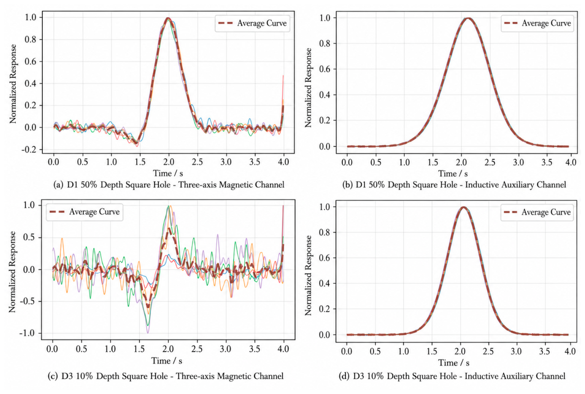
To evaluate the repeatability of the two response types, five repeated scans were conducted for each defect. Figure 4 presents the repeated response curves of representative defects obtained under identical controlled conditions. The magnetic curves show a clear reduction in response strength and increased dispersion for the shallow defect, whereas the inductive curves retain a consistent local response among the repeated scans. These observations describe different channel-specific response characteristics and are not intended as a direct performance ranking between the two sensing mechanisms.
Figure 4.
Repeatability curves of representative defects under five repeated scans: (a) magnetic-channel responses of D1; (b) inductive-channel responses of D1; (c) magnetic-channel responses of D3; and (d) inductive-channel responses of D3. The colored solid lines represent the five repeated scans, and the dashed line represents their average response.
To quantitatively evaluate the channel-specific response strength and repeatability, the response amplitude and coefficient of variation were calculated for each defect based on five repeated scans. The statistical results are listed in Table 3.
Table 3.
Repeatability statistics of dual-channel response amplitudes.
As shown in Table 3, the magnetic response amplitude decreases as the square-hole depth decreases. The average magnetic amplitudes of D1, D2, and D3 are 675.0, 360.1, and 98.5 a.u., respectively. This result confirms that the resultant magnetic response can reflect the depth variation of square-hole defects. However, the magnetic coefficient of variation increases from 2.83% for D1 to 6.61% for D3, indicating that the magnetic response becomes less stable under shallow-defect conditions.
The inductive response also varied among the tested defects, while its repeated-scan dispersion remained low. For D3, the inductive amplitude was a.u., and the corresponding coefficient of variation was 0.23%. The inductive-channel coefficients of variation for D1–D4 were all below 0.25%, indicating stable repeatability under the present controlled scanning conditions. This low dispersion supports the use of the inductive response as auxiliary information when the shallow-defect magnetic response becomes weak. However, repeatability alone does not establish an equivalent or superior capability for representing defect-depth variation.
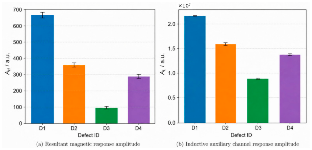
Figure 5 presents the response-amplitude trends of the two channels. Because the magnetic and inductive channels have different sensing mechanisms and output scales, their numerical amplitudes are not used for direct cross-channel ranking. Instead, the magnetic results are used to evaluate the depth-related leakage-field trend, while the inductive results are used to evaluate the repeatability of the supplementary local response.
Figure 5.
Channel-specific response-amplitude trends for the four defects: (a) resultant magnetic response amplitude; (b) inductive auxiliary-channel response amplitude. Error bars represent the standard deviation of five repeated scans (n = 5).
3.3. Channel-Specific Signal-to-Noise Ratio Characteristics
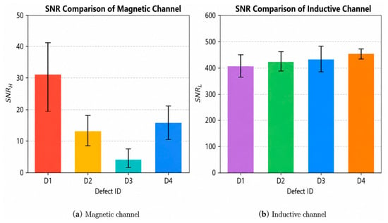
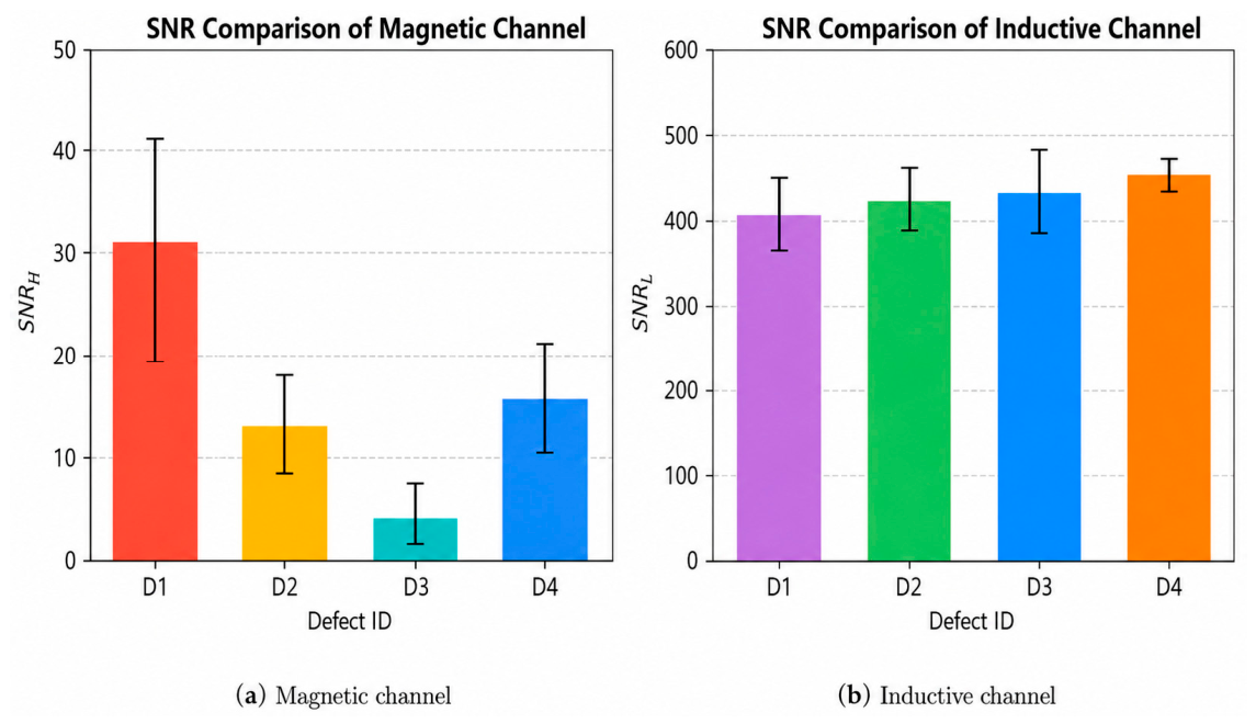
Because the two sensing channels have different sensing mechanisms, output scales, and background-noise characteristics, their SNR values should be interpreted within each channel rather than used for direct absolute ranking between the channels. The SNR was calculated to evaluate the strength of each defect response relative to the corresponding channel-specific baseline noise. The statistical results are summarized in Table 4.
Table 4.
Channel-specific signal-to-noise ratio statistics for the four defects.
The magnetic SNR decreases significantly with the reduction in square-hole depth. For D1, the average magnetic SNR is 30.5. When the defect depth decreases to 30%, the magnetic SNR decreases to 13.3. For the 10% depth shallow defect D3, the magnetic SNR further decreases to 4.7, indicating that the shallow defect produces a weak magnetic response relative to the background fluctuation.
The inductive channel retained a high channel-specific SNR for all four defects. For D3, the average inductive SNR was 434.4, indicating that the local inductive response remained large relative to its own baseline fluctuation under the shallow-defect condition. This result supports the role of the inductive channel as a stable auxiliary sensing channel when the magnetic response becomes weak. However, the numerical SNR values of the two channels cannot be directly ranked because their output units, dynamic ranges, sensing mechanisms, and noise characteristics are different. In particular, the high inductive SNR does not demonstrate that the inductive channel is superior to the magnetic channel, nor does it show that the inductive response can independently replace the depth-related information provided by the magnetic flux leakage response.
Figure 6 presents the channel-specific SNR results. The magnetic SNR decreases markedly for the shallowest defect, whereas the inductive SNR remains high relative to the inductive channel’s own baseline noise. These trends demonstrate complementary response characteristics rather than the absolute superiority of either channel.
Figure 6.
Channel-specific signal-to-noise ratio results for the four defects: (a) magnetic channel; and (b) inductive channel. Error bars represent the standard deviation of five repeated scans (n = 5).
3.4. Peak Position Offset and Spatial Registration
Because the magnetic sensor and the PCB planar coil are installed at different positions on the detection board, their response peaks to the same defect do not appear at exactly the same sampling point. The peak positions of the resultant magnetic response and the inductive response were extracted from the five repeated scans, and the peak-position offset was calculated. The statistical results are listed in Table 5.
Table 5.
Measured pre-registration peak-position offsets between the magnetic and inductive responses.
At the scanning speed of 10 mm/s and sampling frequency of 100 Hz, the confirmed center-to-center distance of 1.79 mm corresponded to a nominal geometric offset of 17.9 sampling intervals. The measured pre-registration peak-position offsets were 12.8 ± 1.8, 9.4 ± 3.6, and 12.4 ± 2.8 sampling points for D1, D2, and D4, respectively. These measured offsets were relatively stable among the five repeated scans but did not exactly equal the nominal geometric offset. This difference is expected because the extrema of the magnetic and inductive response curves are determined not only by the physical sensor separation but also by the different sensing mechanisms, response profiles, defect geometry, background fluctuation, and peak-extraction procedure. Therefore, the values in Table 5 represent scan-specific pre-registration peak-position offsets used for signal alignment rather than direct measurements of the sensor-to-coil center distance or residual errors after registration.
For D3, the measured pre-registration peak-position offset was sampling points. Although its mean value was relatively close to the nominal geometric offset of 17.9 sampling intervals, the standard deviation was substantially larger than those obtained for D1, D2, and D4. The magnetic-channel of D3 was only 4.7, and the weak magnetic response made the extracted magnetic extremum highly sensitive to background fluctuation and local noise. By comparison, the inductive peak time was more repeatable, with a mean of and a standard deviation of . However, the stable inductive peak alone does not establish that the scan-specific alignment is accurate, because the measured offset still depends on the unstable magnetic peak position. Therefore, the large scatter of D3 demonstrates substantial uncertainty in registration based on a single pair of extrema under shallow-defect conditions.
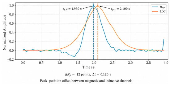
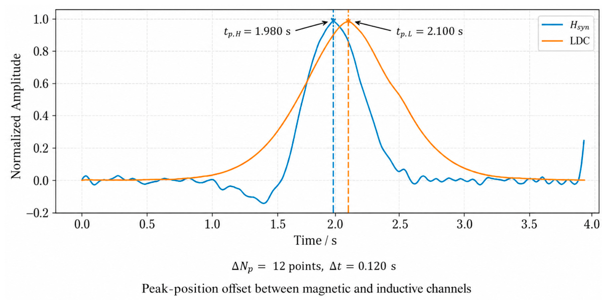
Figure 7 illustrates the peak-position offset between the magnetic and inductive responses. After estimating the offset, one channel can be shifted along the sampling axis to align the dual-channel responses to the same defect region. This spatial registration provides a position-consistent basis for subsequent dual-channel feature construction.
Figure 7.
Schematic illustration of the pre-registration peak-position offset between the magnetic and inductive responses. The blue and orange vertical dashed lines denote the peak positions of the magnetic and inductive responses, respectively.
4. Discussion
4.1. Complementary Characteristics of the Magnetic and Inductive Channels
The experimental results indicate that the magnetic and inductive channels provide different but complementary responses to the tested defects. For the tested square-hole defects, the resultant magnetic response exhibited a pronounced depth-dependent trend. As the depth ratio decreased from 50% for D1 to 10% for D3, the average magnetic amplitude decreased from 675.0 to 98.5 a.u., while the average magnetic SNR decreased from 30.5 to 4.7. The magnetic coefficient of variation also increased from 2.83% to 6.61%. These results show that the magnetic channel retained useful information associated with the variation in defect depth, but its response strength and repeatability deteriorated for the shallowest defect.
This behavior is consistent with the magnetic flux leakage sensing mechanism. A deeper material discontinuity produces a stronger disturbance in the local magnetic-reluctance distribution and consequently generates a stronger leakage magnetic field. When the defect is shallow, the leakage-field disturbance becomes weaker relative to background-field fluctuation, lift-off variation, sensor posture, and local geometric effects. The magnetic peak amplitude and peak position therefore become more susceptible to noise under shallow-defect conditions.
The inductive channel exhibited a different response characteristic. For D3, its average SNR remained 434.4 and its coefficient of variation was 0.23%, indicating that the PCB coil continued to provide a stable response when the magnetic response became weak. This inductive response originates from changes in the electromagnetic coupling between the planar coil and the conductive ferromagnetic surface. It is therefore affected by local material continuity, permeability, conductivity, lift-off, and defect geometry rather than being a second measurement of the leakage magnetic field.
The numerical SNR values of the two channels should not be directly ranked because the channels have different sensing mechanisms, output units, dynamic ranges, and background-noise characteristics. In particular, the high SNR of the inductive channel does not establish that it has the same capability as the magnetic channel for representing defect-depth variation. The present experiments show that the inductive response remained stable for the shallow defect, but they do not demonstrate that the inductive channel alone can provide complete defect-depth characterization or replace the magnetic flux leakage measurement.
The necessity of the dual-channel configuration therefore arises from the different information supplied by the two sensing mechanisms. The magnetic channel contributes a leakage-field response that varies markedly with the depths of the tested square-hole defects, whereas the inductive channel supplies a stable auxiliary indication when the magnetic response becomes weak. After spatial registration, these two types of features can be associated with the same defect region. The resulting feature description is more complete than that obtained from the magnetic channel alone, although the present study does not claim that the dual-channel method has already achieved automatic defect classification or field-level detection performance.
The benefit of the dual-channel configuration should be understood as improved defect observability and information redundancy rather than direct amplification of the raw signal from either channel. When the magnetic response is sufficiently strong, it provides a pronounced leakage-field trend associated with the depths of the tested square-hole defects. When the magnetic response becomes weak and its peak position becomes sensitive to background fluctuation, as observed for D3, the inductive channel can still provide a stable supplementary indication of the local defect region. The combination therefore reduces dependence on a single response mechanism and decreases the risk that a weak or unstable response in one channel will result in an incomplete interpretation. However, because the present study did not include a systematic no-defect dataset or a classification experiment, this improvement is described in terms of complementary observability and repeated-scan robustness rather than a quantitatively demonstrated reduction in false-alarm or missed-detection rates.
A further potential advantage of the dual-channel configuration is the reduction in ambiguity between defects located on different surfaces of a ferromagnetic component. Conventional magnetic flux leakage measurements can respond to defects on both the near and far surfaces, and different combinations of defect position and geometry may produce similar leakage-field characteristics [2]. The inductive channel provides an additional electromagnetic-coupling response that is more directly influenced by the material condition close to the inspection surface. Therefore, combining the leakage-field response with the inductive response may provide additional information for distinguishing near-side and far-side defects. Nevertheless, all defects investigated in the present study were located on the inner surface, which was also the inspection surface. The current results therefore do not constitute experimental validation of inner- and outer-surface defect classification. Paired experiments using defects with controlled geometries on both surfaces will be required before this capability can be quantitatively established.
4.2. Necessity of Spatial Registration
The fixed center-to-center distance between the MLX90393 and the PCB coil provides a nominal geometric reference for spatial registration. Under the present scanning conditions, the 1.79 mm separation corresponds to 17.9 sampling intervals. However, the measured pre-registration peak-position offsets for D1, D2, and D4 were , , and sampling points, respectively. The measured peak offsets did not exactly coincide with the geometric reference because the peak of each response is affected by the channel-specific sensing mechanism, response shape, defect geometry, noise, and extremum-extraction procedure. The geometric separation should therefore be interpreted as a nominal registration reference, whereas the values reported in Table 5 are the measured scan-specific offsets used to perform the alignment.
This result confirms that spatial registration is necessary before dual-channel feature construction. If the two channels are directly fused without considering the spatial offset, the extracted magnetic and inductive features may correspond to different physical positions on the specimen. This position mismatch may reduce the reliability of feature-level fusion, especially when the defect response region is narrow or when multiple local disturbances exist along the scanning path. By estimating the peak-position offset and shifting one channel along the sampling axis, the two responses can be aligned to the same defect region, providing a position-consistent basis for subsequent feature analysis.
For the 10% depth shallow defect D3, the measured pre-registration offset was sampling points. This large scatter arose primarily because the weak magnetic response made the magnetic extremum sensitive to background fluctuation and noise. Although the inductive response remained comparatively stable, that stability does not independently determine the correct spatial offset when the magnetic peak position is uncertain. Consequently, the present peak-based registration procedure is suitable for scan-specific response association under the controlled conditions used in this study, but it cannot be regarded as having completely eliminated shallow-defect localization error or as being highly reliable for all shallow defects. More robust registration approaches, including cross-correlation, template matching, window-constrained alignment, and calibration-based registration using the known sensor separation, scanning speed, and sampling frequency, should be investigated in future work.
Although the measured peak-position offset becomes unstable when the magnetic extremum is weak, the confirmed sensor geometry provides an independent physical reference. The center-to-center distance of 1.79 mm corresponds to a nominal geometric offset of 17.9 sampling intervals under the present scanning conditions. Unlike the measured peak-position offset, this geometric reference does not depend on the stability of an individual magnetic extremum. It can therefore be used as a physical prior, an initial alignment value, or the center of a constrained search window when peak-based registration becomes unreliable. A more robust implementation may combine this geometric prior with cross-correlation, template matching, or other window-constrained methods. However, the current results were obtained using the measured scan-specific peak-position offsets, and a geometry-constrained hybrid registration algorithm was not independently implemented or validated in this study. Therefore, the 17.9-sampling-interval value is interpreted as a nominal physical reference rather than evidence that the D3 localization uncertainty has already been eliminated.
4.3. Applicability to Ferromagnetic Components and Scope of the Proposed Method
The proposed sensing and spatial-registration framework is based on the magnetic-flux-leakage and electromagnetic-coupling responses of conductive ferromagnetic materials and is not inherently restricted to a particular pipe diameter or pipeline geometry. In the present study, a laboratory pipeline inspection platform was used as a controlled validation configuration, in which the Q235 defect specimen was installed at the internal inspection position and the motor-driven detection board scanned axially along the inner inspection surface. Therefore, the pipeline platform represents the experimental validation environment of this study rather than the exclusive application boundary of the proposed method.
Within this controlled configuration, the contribution of the proposed method comprises three connected aspects. First, an MLX90393 three-axis magnetic sensor and a PCB planar spiral coil were integrated into a compact magnetic–inductive detection board. Second, the physical separation between the two sensing units was explicitly considered through nominal geometric-offset analysis and scan-specific spatial registration. Third, the registered responses were used to evaluate the complementary roles of the two channels under shallow-defect conditions. The novelty therefore lies in the integration, spatial correspondence, and complementary characterization strategy rather than in presenting magnetic flux leakage or inductive sensing as a newly developed individual sensing principle.
The experimental results demonstrate the feasibility of this strategy for the tested Q235 defect specimen under controlled conditions. The magnetic channel exhibited a pronounced response trend with square-hole depth, whereas the inductive channel maintained stable repeatability and a high channel-specific SNR when the shallow-defect magnetic response became weak. After spatial registration, the two response types could be associated with the same local defect region, providing a broader feature description than the magnetic response alone. These results support the proposed complementary sensing strategy, but they should not be extrapolated directly to other component geometries or practical field conditions without further experimental validation.
In principle, the compact dual-channel architecture may be adapted to other ferromagnetic components with accessible scanning surfaces, such as steel plates, storage-tank walls, and rail-like components. The sensor-to-coil separation can be represented in the corresponding spatial sampling coordinate using the scanning speed and sampling frequency, while the two response types can be associated through the same geometry-aware registration concept. Nevertheless, such transfer requires application-specific redesign and calibration of the magnetization structure, sensing trajectory, lift-off, scanning speed, sampling frequency, and probe coverage. Because the present experiments were conducted only on a laboratory pipeline inspection platform using a Q235 specimen, applicability to other ferromagnetic components remains a potential extension rather than an experimentally validated conclusion of this study.
4.4. Limitations and Future Work
Although the present results demonstrate complementary magnetic and inductive responses under controlled conditions, the scope of the validation remains limited. The experiments were conducted using machined defects installed at the internal inspection position of a laboratory pipeline platform. The defect openings were located on the inner surface, and the detection board scanned on the same side as the openings. This arrangement reproduces the internal installation position and spatial constraints of pipeline inspection, but it does not reproduce the full range of conditions encountered in an in-service pipeline. In particular, irregular corrosion morphology, surface deposits, coatings, fluid-related effects, complex pipe curvature, mechanical vibration, and other field disturbances were not included.
The current specimen had a wall thickness of 10 mm, and only four defect configurations were investigated. The experiments did not systematically vary wall thickness, defect length, defect width, defect opening area, orientation relative to the scanning direction, or irregular material-loss morphology. Consequently, the present results cannot establish the minimum detectable defect size or the scalability of the method across different pipe-wall and defect dimensions. Future experiments should include additional wall thicknesses, systematically varied defect lengths and widths, different opening areas, irregular corrosion profiles, and different relationships between the defect dimensions and probe coverage. These experiments will be required to evaluate defect-size sensitivity and the scalability of the compact dual-channel configuration.
The operating conditions were also controlled. The present experiments used a scanning speed of 10 mm/s, a 1 mm lift-off, and a fixed magnetization arrangement. The effects of scanning-speed variation, lift-off fluctuation, magnetization variation, sensor posture, pipe curvature, surface roughness, coatings, and mechanical vibration were not independently evaluated. Future work should therefore investigate these variables individually and in combination to determine their effects on the magnetic response, inductive response, repeatability, and spatial correspondence between the two channels.
A further limitation concerns spatial registration under shallow-defect conditions. For D3, the measured pre-registration peak-position offset was sampling points. The large scatter arose primarily from the weak magnetic response and the resulting sensitivity of the magnetic extremum to background fluctuation and noise. This result demonstrates that alignment based on a single magnetic extremum has substantial uncertainty for shallow defects. The current method is therefore suitable for scan-specific response association under the present controlled conditions, but it should not be interpreted as having completely eliminated shallow-defect localization error. Future studies should investigate cross-correlation, template matching, window-constrained alignment, and calibration-based registration using the known sensor separation, scanning speed, and sampling frequency.
Finally, the present study focused on response characterization rather than complete detection, classification, or inverse reconstruction of unknown defect dimensions. The known lengths, widths, diameters, and depths of D1–D4 were used as controlled geometric references for evaluating the relationships between defect geometry and the extracted dual-channel response features. No inverse model was developed to estimate unknown defect length, width, or depth from the measured signals. A systematic no-defect dataset and a series of defects with progressively reduced dimensions were also not included. Therefore, detection probability, false-alarm rate, missed-detection rate, classification accuracy, minimum detectable defect size, and defect-dimension reconstruction error were not determined in the present study. All four tested defects produced identifiable local response variations under the current magnetization, lift-off, scanning, and sampling conditions; however, this result does not establish a universal detection threshold. The minimum detectable defect size depends jointly on defect geometry, wall thickness, magnetization level, lift-off, sensor sensitivity, background noise, scanning speed, and spatial sampling interval. Similarly, an acceptable distance between the two sensing units cannot be specified using a universal fixed multiple of the defect size. In the present configuration, the 1.79 mm sensor-to-coil center distance was substantially smaller than the 20 mm characteristic dimension of the tested defect openings, and both sensing trajectories traversed the local defect regions. Future work should include no-defect measurements, systematically varied defect dimensions, inner- and outer-surface defect pairs, and expanded calibration datasets before threshold-based detection, defect classification, or inverse dimensional reconstruction is evaluated. Accordingly, the conclusions of the present study are limited to the feasibility of compact magnetic–inductive integration, spatial correspondence under controlled scanning conditions, and complementary characterization of the tested defects.
5. Conclusions
This study developed a compact magnetic–inductive dual-channel inspection method with spatial registration for defect characterization in ferromagnetic materials and evaluated it through controlled experiments on a laboratory pipeline inspection platform. A Q235 defect specimen was installed at the internal inspection position of the pipe, and the dual-channel detection board was driven axially along the inner inspection surface. The MLX90393 three-axis magnetic sensor acquired the magnetic-flux-leakage response, while the PCB planar spiral coil and LDC1612 acquired the inductive response. The purpose of the dual-channel configuration was to obtain different but complementary response information rather than to demonstrate the superiority of either sensing channel. The main conclusions are as follows.
- The resultant magnetic response exhibited a pronounced depth-dependent trend for the tested square-hole defects. As the depth ratio decreased from 50% to 10%, the average magnetic amplitude decreased from 675.0 to 98.5 a.u., and the average magnetic SNR decreased from 30.5 to 4.7. The magnetic channel therefore retained information associated with defect-depth variation, although its response became weaker and less repeatable for the shallowest defect.
- The inductive channel provided a stable auxiliary response under the shallow-defect condition. For the 10% depth square-hole defect D3, the inductive amplitude was a.u., the average SNR was 434.4, and the coefficient of variation was 0.23%. These results demonstrate stable inductive repeatability but do not indicate that the inductive channel is absolutely superior to the magnetic channel or that it can independently replace the depth-related leakage-field information.
- The 1.79 mm center-to-center separation between the magnetic sensor and the PCB coil corresponded to a nominal geometric offset of 17.9 sampling intervals under the present scanning conditions. The measured pre-registration peak-position offsets were , , and sampling points for D1, D2, and D4, respectively. These measured offsets were used to associate the magnetic and inductive response regions before dual-channel comparison and should not be interpreted as post-registration residual errors. For D3, the measured offset was sampling points. The large scatter demonstrates that registration based on a single pair of extrema has substantial uncertainty when the shallow-defect magnetic response is weak.
Overall, the magnetic and inductive channels provide different and complementary information. The magnetic channel provides a pronounced response trend associated with the depths of the tested square-hole defects, whereas the inductive channel supplies a stable auxiliary response when the shallow-defect magnetic response becomes weak. The inductive channel’s high SNR does not independently establish complete defect-depth characterization, and neither channel should be regarded as replacing the other. After spatial registration, their features can be associated with the same local defect region, providing a more complete description of the tested defect responses than either response type considered alone. Nevertheless, the present results are limited to controlled experiments using a Q235 defect specimen installed on a laboratory pipeline platform and do not constitute comprehensive validation for other ferromagnetic components or practical field conditions. The current results also do not establish inner- and outer-surface defect classification, minimum detectable defect size, or inverse reconstruction of unknown defect dimensions. Future studies should therefore include no-defect samples, paired inner- and outer-surface defects, irregular corrosion morphologies, additional wall thicknesses and systematically varied defect dimensions, variable lift-off and scanning speeds with correspondingly adjusted sampling frequencies, complex curvature, vibration, coatings, and realistic pipeline operating disturbances. Application-specific redesign and validation will also be required before the proposed sensing and registration framework is extended to other ferromagnetic components.
Supplementary Materials
The following supporting information can be downloaded at: https://www.mdpi.com/article/10.3390/machines14080867/s1, Supplementary_Data_English.xlsx: LDC1612 IDRIVE parameter-test results, MLX90393 data acquired with the LDC1612 IDRIVE setting code set to 19, five repeated dual-channel scanning datasets, frequency-domain features, and extracted dual-channel feature summary.
Author Contributions
Conceptualization, J.Q. and S.L.; methodology, J.Q.; software, J.Q.; validation, J.Q.; formal analysis, J.Q.; investigation, J.Q.; resources, S.L.; data curation, J.Q.; writing—original draft preparation, J.Q.; writing—review and editing, S.L.; visualization, J.Q.; supervision, S.L.; project administration, S.L.; funding acquisition, S.L. All authors have read and agreed to the published version of the manuscript.
Funding
This research was funded by the National Natural Science Foundation of China, grant number 62573098, and the Liaoning Provincial Science and Technology Plan Project, grant number 2025JH2/101300049.
Data Availability Statement
The data presented in this study are available from the corresponding author upon reasonable request. The repeated scanning data and extracted features are provided in the Supplementary Materials.
Acknowledgments
The authors would like to thank the laboratory members for their assistance with the experimental setup, repeated scanning experiments, and data acquisition.
Conflicts of Interest
The authors declare no conflicts of interest.
Abbreviations
The following abbreviations are used in this manuscript:
| MFL | Magnetic flux leakage |
| NDT | Nondestructive testing |
| PCB | Printed circuit board |
| LDC | Inductance-to-digital converter |
| SNR | Signal-to-noise ratio |
| CV | Coefficient of variation |
| LC | Inductance–capacitance |
| a.u. | Arbitrary unit |
| IN0 | Input channel 0 |
References
- Xie, M.; Tian, Z. A review on pipeline integrity management utilizing in-line inspection data. Eng. Fail. Anal. 2018, 92, 222–239. [Google Scholar] [CrossRef] [Scilit]
- Shi, Y.; Zhang, C.; Li, R.; Cai, M.; Jia, G. Theory and application of magnetic flux leakage pipeline detection. Sensors 2015, 15, 31036–31055. [Google Scholar] [CrossRef] [Scilit] [PubMed]
- Ma, Q.; Tian, G.Y.; Zeng, Y.; Li, R.; Song, H.; Wang, Z.; Gao, B.; Zeng, K. Pipeline in-line inspection method, instrumentation and data management. Sensors 2021, 21, 3862. [Google Scholar] [CrossRef] [Scilit] [PubMed]
- Feng, B.; Wu, J.; Tu, H.; Tang, J.; Kang, Y. A review of magnetic flux leakage nondestructive testing. Materials 2022, 15, 7362. [Google Scholar] [CrossRef] [Scilit] [PubMed]
- Huang, S.; Peng, L.; Sun, H.; Li, S. Deep learning for magnetic flux leakage detection and evaluation of oil and gas pipelines: A review. Energies 2023, 16, 1372. [Google Scholar] [CrossRef] [Scilit]
- Dutta, S.M.; Ghorbel, F.H.; Stanley, R.K. Dipole modeling of magnetic flux leakage. IEEE Trans. Magn. 2009, 45, 1959–1965. [Google Scholar] [CrossRef] [Scilit]
- Li, Y.; Wilson, J.; Tian, G.Y. Experiment and simulation study of 3D magnetic field sensing for magnetic flux leakage defect characterisation. NDT E Int. 2007, 40, 179–184. [Google Scholar] [CrossRef] [Scilit]
- Tang, J.; Wang, R.; Qiu, G.; Hu, Y.; Kang, Y. Mechanism of magnetic flux leakage detection method based on the slotted ferromagnetic lift-off layer. Sensors 2022, 22, 3587. [Google Scholar] [CrossRef] [Scilit] [PubMed]
- Qu, F.; Zhang, X.; Li, Y.; Wang, Y.; Wang, C. Design and performance study of a magnetic flux leakage pig for subsea pipeline defect detection. J. Mar. Sci. Eng. 2025, 13, 1462. [Google Scholar] [CrossRef] [Scilit]
- García-Martín, J.; Gómez-Gil, J.; Vázquez-Sánchez, E. Non-destructive techniques based on eddy current testing. Sensors 2011, 11, 2525–2565. [Google Scholar] [CrossRef] [Scilit] [PubMed]
- Sophian, A.; Tian, G.Y.; Fan, M. Pulsed eddy current non-destructive testing and evaluation: A review. Chin. J. Mech. Eng. 2017, 30, 500–514. [Google Scholar] [CrossRef] [Scilit]
- Rifai, D.; Abdalla, A.N.; Ali, K.; Razali, R. Giant magnetoresistance sensors: A review on structures and non-destructive eddy current testing applications. Sensors 2016, 16, 298. [Google Scholar] [CrossRef] [Scilit] [PubMed]
- Machado, M.A.; Rosado, L.S.; Mendes, N.M.M.; Miranda, R.M.; dos Santos, T.G. Eddy currents probe design for NDT applications: A review. Sensors 2024, 24, 5819. [Google Scholar] [CrossRef] [Scilit] [PubMed]
- Rosado, L.S.; Cardoso, F.A.; Cardoso, S.; Ramos, P.M.; Freitas, P.P.; Piedade, M. Eddy currents testing probe with magneto-resistive sensors and differential measurement. Sens. Actuators A Phys. 2014, 212, 58–67. [Google Scholar] [CrossRef] [Scilit]
- Ma, Q.; Gao, B.; Tian, G.Y.; Yang, C.; Xie, L.; Chen, K. High sensitivity flexible double square winding eddy current array for surface micro-defects inspection. Sens. Actuators A Phys. 2020, 309, 111844. [Google Scholar] [CrossRef] [Scilit]
- Long, C.; Zhang, N.; Tao, X.; Tao, Y.; Ye, C. Resolution enhanced array ECT probe for small defects inspection. Sensors 2023, 23, 2070. [Google Scholar] [CrossRef] [Scilit] [PubMed]
- Deng, Z.; Yang, C.; Li, Y.; Tian, G.Y.; Peng, L. Effects of curvature radius on flexible eddy current array sensors for the curved surface of metal components. Front. Phys. 2022, 10, 988009. [Google Scholar] [CrossRef] [Scilit]
- Lu, M.; Zhu, W.; Yin, L.; Peyton, A.J.; Yin, W.; Qu, Z. Reducing the lift-off effect on permeability measurement for magnetic plates from multifrequency induction data. IEEE Trans. Instrum. Meas. 2018, 67, 167–174. [Google Scholar] [CrossRef] [Scilit]
- Kaziz, S.; Romano, P.; Imburgia, A.; Ala, G.; Sghaier, H.; Flandre, D.; Tounsi, F. PCB-based planar inductive loops for partial discharges detection in power cables. Sensors 2023, 23, 290. [Google Scholar] [CrossRef] [Scilit] [PubMed]
- Kim, B.; Han, S.; Kim, K. Planar spiral coil design for a pulsed induction metal detector to improve the sensitivities. IEEE Antennas Wirel. Propag. Lett. 2014, 13, 1501–1504. [Google Scholar] [CrossRef] [Scilit]
- Gao, B.; Li, X.; Woo, W.L.; Tian, G.Y. Quantitative validation of eddy current stimulated thermal features on surface crack. NDT E Int. 2017, 85, 1–12. [Google Scholar] [CrossRef] [Scilit]
- Dodd, C.V.; Deeds, W.E. Analytical solutions to eddy-current probe-coil problems. J. Appl. Phys. 1968, 39, 2829–2838. [Google Scholar] [CrossRef] [Scilit]
- Nara, T.; Fujieda, M.; Gotoh, Y. Non-destructive inspection of ferromagnetic pipes based on the discrete Fourier coefficients of magnetic flux leakage. J. Appl. Phys. 2014, 115, 17E509. [Google Scholar] [CrossRef] [Scilit]

Disclaimer/Publisher’s Note: The statements, opinions and data contained in all publications are solely those of the individual author(s) and contributor(s) and not of MDPI and/or the editor(s). MDPI and/or the editor(s) disclaim responsibility for any injury to people or property resulting from any ideas, methods, instructions or products referred to in the content. |
© 2026 by the authors. Licensee MDPI, Basel, Switzerland. This article is an open access article distributed under the terms and conditions of the Creative Commons Attribution (CC BY) license.