


Abstract
Redundant manipulators offer greater flexibility in executing complex trajectory-tracking tasks in industrial applications, owing to their additional degrees of freedom (DOFs). However, their inverse kinematics (IK) remains computationally expensive, limiting their practical application. By combining the joint parameterization method (JPM) and the stationary point solver (SPS), the JPSP-IK framework is proposed to provide closed-form joint solutions while significantly reducing the computational burden. JPM treats the redundant variables as free parameters and analytically reconstructs the remaining joints in closed form from these variables and the target end-effector pose, thereby reducing the original full-space IK problem to a low-dimensional redundancy-resolution problem. On this basis, the SPS is developed to efficiently determine the redundant variables with respect to the secondary objective, considering joint-limit avoidance and motion smoothness, and the complete joint solution is analytically reconstructed through the analytical mapping derived by the JPM. Validation and comparative experiments demonstrate that JPSP-IK achieves substantially lower computation times than representative full-space and JPM-based IK methods.
1. Introduction
Redundant manipulators have gained significant attention in robotics, as their additional degrees of freedom (DOFs) offer enhanced flexibility and dexterity for complex tasks [1,2,3]. Unlike non-redundant manipulators, they are capable of accomplishing the primary end-effector (EE) pose task while simultaneously satisfying secondary objectives [4], such as joint-limit avoidance, motion smoothness, and obstacle avoidance. Owing to these capabilities, the redundant manipulators have been widely deployed in challenging environments [5,6], including the Tiangong space station [2] and nuclear fusion reactors [3,7]. In such scenarios, operations, including path planning, trajectory tracking, and EE positioning, all rely on efficient and accurate inverse-kinematics (IK) solutions. However, the additional DOFs also lead to an infinite number of joint configurations that realize the same EE pose. The key challenge is therefore to determine a joint configuration that not only achieves the target pose but also satisfies secondary tasks [4]. Existing methods for solving the IK of redundant manipulators can be generally categorized into numerical methods [8,9,10,11,12], optimization methods [13,14,15,16,17,18,19], learning-based methods [20,21,22,23], and analytical methods [4,24,25,26].
Numerical methods are applicable to a broad range of manipulator structures, and Jacobian-based methods are among the most widely used approaches [8,27,28,29]. These methods use the Jacobian matrix to establish the mapping between joint velocities and EE velocities. For redundant manipulators, the non-square Jacobian is handled using the pseudoinverse [30] or an extended-inverse technique [10]. Although these methods are computationally efficient, they remain sensitive to initialization, may converge to locally feasible yet suboptimal configurations [31], and are susceptible to singularities [32]. To improve the numerical stability near singular configurations, the damped least-squares (DLS) method [9] introduces a damping factor into the inversion process. However, this strategy often comes at the cost of a reduced convergence speed and degraded solution accuracy [33]. Moreover, Jacobian-based methods typically return a single solution rather than multiple feasible configurations, which may limit the exploitation of kinematic redundancy for secondary objectives.
Optimization methods formulate the IK as the minimization of a task-dependent objective in the joint space. Representative approaches include gradient-based [34] and population-based methods [14,15,16,17,19,35]. Gradient-based methods, such as gradient descent (GD), update the joint vector iteratively using local gradient information. However, their performance is often sensitive to initialization [36], step-size selection, and the local objective landscape [37]. This sensitivity may lead to a slow convergence and suboptimal configurations [38]. In contrast, population-based methods, such as particle swarm optimization (PSO) [13,14,16], differential evolution (DE) [18,35], and genetic algorithms (GAs) [15,19], can provide a better global exploration capability [39] and greater flexibility in handling nonlinear objectives and irregular constraints. As a result, they are less dependent on a single initial guess and may obtain higher-quality solutions than purely local gradient-based search [39]. However, the repeated evaluation of large populations incurs a substantial computational cost, which limits their suitability for real-time control [40]. To alleviate this limitation, hybrid approaches have been explored. Koker and Çakar [41] proposed a hybrid architecture combining neural networks with heuristic searches, demonstrating a significantly higher computational efficiency than pure optimization methods. Starke et al. [42] developed a hybrid strategy that combines genetic algorithms with particle swarm optimization for IK, showing that hybrid metaheuristics can improve the robustness and solution quality compared with a single-strategy evolutionary search. Nevertheless, these approaches still rely heavily on iterative optimization and repeated fitness evaluations, and, thus, do not fully remove the computational burden of high-dimensional redundant IK.
Learning-based methods have also been extensively investigated for the IK of redundant manipulators. By learning the relationship between end-effector poses and joint configurations from large datasets, neural-network-based methods enable fast online inference [21,43,44]. In addition, recurrent architectures [45] and reinforcement learning (RL) methods [22] have also been explored for IK with multiple secondary objectives. However, many conventional deterministic learning-based approaches return only one joint configuration for a given target pose [46], which does not adequately represent the one-to-many nature of redundant inverse kinematics [20]. To address this, generative architectures such as IKFlow [20] and GANs [23] have been proposed. These methods can efficiently generate multiple IK candidates for a given target pose. Nevertheless, the generated configurations are typically approximate and may still require numerical refinement or local optimization to eliminate the pose error [20]. Therefore, achieving a consistently high pose accuracy while retaining efficient online inference remains challenging.
Analytical IK methods exploit the geometric and kinematic structure to derive closed-form solutions and offer a high computational efficiency [47,48]. Classical analytical approaches rely on specific geometric conditions, as exemplified by Pieper’s criterion and Paul’s criterion [49,50]. Consequently, these methods are primarily applicable to non-redundant manipulators with specific joint-axis arrangements. To extend the analytical IK to redundant manipulators, the joint parameterization method (abbreviated as JPM in this work) [51] can be used to decompose the full joint space into redundant and non-redundant joint variables. Once the redundant variables are specified, the remaining non-redundant variables can be reconstructed analytically. In this way, the original full-space IK is transformed into the problem of determining appropriate redundant variables, namely, redundancy resolution. Therefore, redundancy resolution is a key step for JPM-based IK [24], and various strategies have been developed. The existing studies on redundancy resolution mainly focus on two aspects. The first concerns the selection of appropriate redundant joints. To address the issue, Zaplana and Basanez [24] applied the workspace analysis to select the redundant joints, after which the sub-chain is solved by the Pieper and Paul methods. The selection can also be achieved through GNG clustering [4], which identifies appropriate redundant joints and transforms the redundant manipulator into a non-redundant one. For a specific industrial application, Guo et al. [47] have proposed a hybrid IK method for a tunnel shotcrete redundant manipulator, where WLN provides an approximate solution and the JPM is then used to extract proper redundant joints for analytical refinement. The second aspect concerns the determination of suitable values of the selected redundant variables, for which optimization-based strategies have been widely explored. For example, to enhance the global search capability and alleviate local-minimum issues in GAs, Zeng et al. [52] incorporated a GA–PSO-based strategy before the JPM to optimize the redundant joints. Similarly, Wu et al. [26] have proposed T-IK, which couples redundant-space optimization based on an improved NSGA-II algorithm with an analytical IK solver to enhance the trajectory suitability for general robots. However, these optimization-based redundancy-resolution strategies still require an iterative search and repeated objective evaluations, thereby introducing an additional computational cost.
Compared with purely numerical, optimization-based, and learning-based IK methods, JPM-based analytical methods are particularly attractive for redundant manipulators because the full joint solution is obtained in the closed form, with pose errors at numerical precision. Moreover, by reducing the original IK problem into redundancy resolution in a low-dimensional subspace, the JPM yields multiple feasible solutions and offers a higher computational efficiency. However, in most existing JPM-based frameworks, redundancy resolution is still performed through iterative optimization, which is a major bottleneck for real-time implementation [52]. These redundancy-resolution methods are often sensitive to initialization and may require extensive iterations before a satisfactory solution is obtained [36,37,40]. In this paper, the stationary point solver (SPS) is developed for redundancy resolution. Instead of relying on repeated iterative updates, the SPS determines the redundant variables by solving for the stationary point of a quadratic approximation of the secondary objective. By integrating the JPM with the SPS, a novel inverse kinematics framework for redundant manipulators, termed JPSP-IK, is proposed.
The remainder of this paper is organized as follows: Section 2 describes the proposed JPSP-IK method, including the derivation of IK based on the JPM and the principles of the SPS. Section 3 applies JPSP-IK to two types of manipulators. Section 4 presents comparative experiments on trajectory-tracking tasks. Section 5 provides a detailed discussion on the performance analysis and limitations of JPSP-IK. Section 6 concludes the paper.
2. JPSP-IK Framework for Redundant Manipulators
In this section, the mathematical formulation and workflow of the proposed JPSP-IK framework are introduced, as illustrated in Figure 1. The framework consists of two sequential stages, the joint-space dimensionality reduction by the JPM and redundancy resolution by the SPS. At the k-th trajectory waypoint, the target end-effector pose and the previous joint state are used as inputs. In the first stage, the JPM is adopted to partition the full joint vector q into redundant variables and non-redundant variables . Once is specified, can be obtained in the closed form from the target pose and the redundant variables through the inverse kinematic mapping . In this way, the original problem is reduced from a full-space IK to a low-dimensional redundancy-resolution problem. In the second stage, the SPS determines by solving for the stationary point of a quadratic approximation of the secondary objective. This quadratic approximation is obtained by locally linearizing the full-joint reconstruction mapping with respect to the redundant-variable increment . In this way, the search process avoids costly iterative optimization. Finally, the redundant variables are mapped back through to obtain the complete joint configuration for the current waypoint.
Figure 1.
The theoretical framework of JPSP-IK. For a given end-effector target pose of the k-th waypoint, JPSP-IK generates the current joint state based on the previous joint state and the objective function including joint-limit avoidance and motion smoothness .
2.1. Joint-Space Dimensionality Reduction Based on JPM
This subsection presents the joint-space dimensionality reduction stage based on the joint parameterization method (JPM). First, a unified forward kinematics model is established for general redundant manipulators [53]. Based on the established kinematic model, the JPM reformulates the inverse kinematics problem by treating the redundant variables as independent parameters, such that the non-redundant variables can be analytically reconstructed in the closed form from the target pose. In this way, the original full-space IK problem is transformed into a reduced-dimensional redundancy-resolution problem, which provides the analytical basis for the stationary point solver (SPS) presented in the next subsection.
2.1.1. Forward Kinematics Model
For an n-DOF redundant manipulator, the forward kinematics (FK) establishes the mapping from the joint vector to the end-effector pose. The overall FK is given by the ordered product of the relative homogeneous transformation matrices between adjacent link frames, expressed as follows:
where denotes the end-effector pose, as given in Equation (2), and and represent the orientation and position components, respectively. is the variable of the i-th joint, and denotes the relative transformation from frame to . In this work, each relative transformation matrix is described using six increments [48], as written in Equation (3), where and denote the translational increments along the x-, y-, and z-axes of the frame , respectively, while and denote the rotational increments about the corresponding axes. For each joint, only one of these six increments serves as the joint variable , while the remaining five quantities are constant geometric parameters determined by the manipulator structure. The operators , , , and , in Equation (3) are defined as follows:
2.1.2. Inverse Kinematics via Joint Parameterization Method
Based on the forward kinematics mapping established in the previous section, the inverse kinematics aims to determine the joint vector q that satisfies Equation (1) for a given target end-effector pose . For an n-DOF redundant manipulator, this inverse mapping admits an infinite number of feasible joint configurations because of the kinematic redundancy. To exploit the multiple-solution property of the redundant IK and obtain closed-form solutions, the joint parameterization method (JPM) is adopted. The JPM partitions the full joint vector q into redundant joints and the remaining non-redundant joints , as written in Equation (4). It should be noted that the redundant joints may correspond to joints located at arbitrary positions along the kinematic chain.
By treating as independent free parameters, the forward kinematic mapping in Equation (1) can be rewritten as follows:
where denotes the forward kinematic mapping from the partitioned joint variables to the end-effector pose. Once the redundant variables and the target end-effector pose are specified, the remaining joints become the only unknown variables in Equation (5). By analytically solving Equation (5) for , the remaining joints are obtained as follows:
where denotes the closed-form inverse kinematic mapping from redundant variables and the target end-effector pose to the non-redundant variables. Since the analytical IK may contain multiple solution branches, all real-valued branches are first enumerated for a given and . Branches that violate the joint limits or fail to reconstruct the target pose are discarded. During trajectory tracking, the valid branch with the minimum normalized joint-space distance to the previous joint configuration is selected. For the first waypoint, the initial joint configuration is used as the reference. Therefore, denotes the non-redundant joint vector associated with the selected branch.
Based on the selected , the full joint configuration can be expressed as follows:
where returns the complete n-dimensional joint vector. In this way, the JPM reduces the original full-space IK to a low-dimensional redundancy resolution problem, while ensuring that the joint solution can be obtained in closed form. Different choices of correspond to different joint configurations that realize the same target end-effector pose. However, an arbitrary selection of may lead to undesirable motion behaviors, such as joint-limit violations or motion discontinuities. Therefore, an efficient redundancy resolution mechanism is required to determine according to the secondary objective.
2.2. Redundancy Resolution via Stationary Point Solver
Once the JPM reduces the original full-space IK to redundancy resolution, the remaining task is to determine the redundant variables according to the secondary objective. This task is accomplished by the proposed stationary point solver (SPS).
2.2.1. Secondary Objective Formulation for Redundancy Resolution in Full Joint Space
For a general full-space IK problem, the objective function usually consists of two parts: the primary term and the secondary term. The primary term focuses on the pose error of the end-effector, while the secondary term accounts for the optimization criteria, such as joint-limit avoidance, obstacle avoidance, motion smoothness, and so on [4]. However, in the reduced redundant subspace determined by the JPM, the primary term is no longer required. This is because the JPM obtains the closed-form joint solutions from the redundant variables, and the target end-effector pose is satisfied exactly. Therefore, in the reduced redundant subspace, only the secondary objective function should be formulated. In this paper, two criteria are considered: joint-limit avoidance and motion smoothness. Consequently, the overall objective function can be expressed as the weighted sum of the joint-limit avoidance term [54] and the motion smoothness term [55] as follows:
where and are the weights of the joint-limit avoidance term and the motion smoothness term, respectively. In this work, and . Since the main task is continuous trajectory tracking, a larger weight is assigned to the motion smoothness term to reduce the joint variation between adjacent waypoints. For the -th joint of , and denote the lower limit and upper limit, respectively. and are the values of the i-th joint at the current and previous time steps. is defined as the mean value of and , and n is the number of joints.
Before constructing the reduced-space approximation, its mathematical properties are first examined. By combining Equations (8)–(11), the overall objective function can be rewritten as follows:
where . The partial derivative of with respect to and the Hessian matrix [56] can be written, respectively, as follows:
Since and , all diagonal entries of are positive. Hence, is positive definite, which implies that is strictly convex [57] with respect to q. Therefore, the stationary point of is the unique minimizer of this objective function, and satisfies the following:
This property motivates the stationary-point-based treatment developed in the following subsection.
2.2.2. Reduced-Space Objective and Stationary-Point Solution
Although the secondary objective is originally defined in the full joint space, the actual redundancy resolution is carried out in the reduced space. This is because the complete joint configuration can be analytically obtained from the redundant variables and the target end-effector pose . Consequently, the full space objective in Equation (8) can be defined as the objective with respect to , written as follows:
Consequently, the redundancy resolution problem is reformulated as follows:
To obtain an explicit expression of the objective in terms of , the full-joint reconstruction mapping is linearized with respect to the redundant variable increment around the reference joint configuration as follows:
where . In trajectory tracking, is initialized from the redundant-variable components at the previous waypoint. For the first waypoint, the redundant variables of the initial configuration are selected as . Once is specified, the reference joint configuration can be obtained by the analytical IK as . is the mapping Jacobian matrix, written as follows:
Substituting Equation (18) into Equation (8), the reduced-space objective function can be written as follows:
Because the full joint vector q is implicitly determined by the analytical IK mapping , deriving the corresponding analytical Jacobian involves highly complex symbolic computations that vary with specific robot kinematics. To ensure the generality and computational efficiency of the framework across different manipulator structures, the central finite-difference scheme [58] is applied to approximate the partial derivative, as written in Equation (21).
where is the j-th canonical basis vector, h is a small finite-difference step size, and extracts the i-th component of the reconstructed full joint vector. In this work, h is set to . This value is selected through numerical tests and is fixed throughout all experiments. A larger h may introduce truncation errors because the finite-difference approximation no longer reflects the local linear behavior of the IK mapping.
Since Equation (21) calculates the local variation of the reconstructed joint configuration around , is used as the reference for branch selection at both perturbed points. Specifically, all valid analytical solutions are enumerated at and , and the complete joint configuration with the minimum normalized joint-space distance to is selected at each perturbed point. If either perturbed point admits no valid analytical branch, the corresponding central-difference column cannot be evaluated. In this case, the current waypoint is declared unsuccessful and trajectory execution is terminated.
At this stage, the full space objective is approximated by with respect to the redundant-variable increment. Since is quadratic in q, and q is locally approximated as an affine function of , the resulting surrogate is quadratic in . The SPS therefore determines the redundant-variable increment by imposing the stationary-point condition on this local quadratic surrogate:
Based on the linearization in Equation (18), the two secondary terms and can both be approximated as quadratic functions of the redundant variable increment as follows:
where is a constant diagonal weight matrix defined by the following joint ranges:
Therefore, by combining Equations (23) and (24), the reduced-space objective can be approximated by the following quadratic function with respect to , written as follows:
where the Hessian matrix H and the vector g are defined, respectively, as follows:
Rather than using an outer iterative optimizer, the SPS obtains the redundant-joint increment by imposing the stationary-point condition on Equation (26):
To avoid numerical instability, a Tikhonov-type damping term [59] is introduced. The damping coefficient controls the trade-off between numerical stability and update accuracy. If is too small, the regularization effect becomes weak and the solution may still be unstable. If is too large, the value of will be over-damped, which can reduce the effectiveness of the secondary-objective optimization. In this work, is used, which is also selected through numerical tests. Then, Equation (29) can be rewritten as follows:
Therefore, the redundant variable increment can be obtained by solving the regularized linear system, written as follows:
Note that the weight matrix is defined as a diagonal matrix with positive entries in Equation (25), and is the Jacobian of the full-joint reconstruction mapping. Consequently, with the introduction of the Tikhonov damping term in Equation (30), the regularized Hessian matrix [56] becomes positive definite [57]. Therefore, Equation (31) yields the unique minimizer of the regularized quadratic model of the secondary objective. Since this model is constructed from a local linearization of the nonlinear full-joint reconstruction mapping, is not formally guaranteed to be either a local or global minimizer of the original nonlinear reduced-space objective.
2.2.3. Full Joint Configuration Reconstruction
Once the redundant joint increment is obtained via the SPS, the closed-form full joint configuration can be reconstructed for physical execution. First, the redundant joint variables are updated via a direct forward step:
Subsequently, the updated redundant joint vector is fed into the full-joint reconstruction mapping established by the JPM. The corresponding full joint configuration is directly reconstructed in the closed form as follows:
In summary, the proposed JPSP-IK framework integrates the JPM and the SPS. Unlike traditional full-space numerical solvers that fundamentally rely on prolonged iterative loops, JPSP-IK first reduces the original full-space IK to redundancy resolution in a low-dimensional subspace using the JPM, after which the SPS computes the redundant variables by solving the stationary-point equation of a regularized local quadratic surrogate of the reduced-space secondary objective. The complete closed-form joint configuration is then analytically reconstructed.
3. Application of JPSP-IK to Two Redundant Manipulators
In this section, the proposed JPSP-IK framework is applied to two redundant manipulators with distinct kinematic structures. The first case is an 8-DOF hybrid manipulator with mixed revolute-prismatic joints, representing a structurally more challenging redundancy resolution scenario. The second case is a 9-DOF all-revolute manipulator, representing a more conventional serial-arm configuration. For each manipulator, the redundant-variable selection and the corresponding closed-form reconstruction are first derived, followed by trajectory-tracking simulations that evaluate the applicability of the proposed JPSP-IK.
All algorithms are implemented in Python 3.9.23. PyBullet 3.2.5 is used for forward-kinematics verification and the three-dimensional visualization of the manipulator motion. The experiments are conducted on a desktop computer equipped with an Intel Core i5-14600K CPU and 32 GB of DDR5 memory operating at 5600 MT/s.
3.1. Manipulator A: 8-DOF Hybrid Manipulator
3.1.1. Forward Kinematics of Manipulator A
Manipulator A is an 8-DOF hybrid manipulator in which the second, fourth, and sixth joints are prismatic and the rest are revolute joints, as shown in Figure 2. For each revolute joint , the range is , while, for the prismatic joints , the range is .
Figure 2.
The structure of the 8-DOF hybrid manipulator.
The corresponding forward kinematics parameters with constant offsets, needed for the construction of the relative transformation matrix, are summarized in Table 1.
Table 1.
Forward-kinematics parameters of the 8-DOF hybrid manipulator.
Using the parameters listed in Table 1, the end-effector pose of manipulator A is expressed as follows:
The relative transformation matrices are given below:
Following the methodology presented in Section 2, the analytical IK for the 8-DOF hybrid manipulator is derived. By setting the forward-kinematics matrix in Equation (34) equal to the general end-effector pose matrix defined in Equation (2) and matching the corresponding matrix elements, the position and orientation equations are obtained. The resulting equations, from Equations (35)–(42), constitute the analytical constraints used for the derivation of IK. Since the target end-effector pose is given, the corresponding orientation and position entries, such as , , and , are known constraints in the subsequent derivation.
These equations provide the analytical basis for selecting the redundant variables and sequentially reconstructing the remaining joint variables in the following subsection.
3.1.2. Selection of Redundant Variables
The selection of redundant variables is a key step in the JPM-based analytical IK framework. In this work, the redundant variables are selected according to the following criteria:
- (1)
- First, after fixing the redundant variables, the remaining non-redundant joints should be reconstructed in the closed form from the target end-effector pose.
- (2)
- Second, the analytical expression should be easy to implement and remain numerically stable.
- (3)
- Third, a large portion of the admissible redundant-variable domain should yield real-valued, joint-limit-compliant full-joint configurations.
Based on the manipulator structure, several candidate redundant-variable sets are manually examined. The analytically feasible choices include , , , and . Among the candidate redundant-variable sets examined in this work, these four choices admit the sequential closed-form reconstruction of the remaining joints. The derivation for is given below, while those for the other feasible choices are provided in Appendix A.
For a given and , the expression of is first derived according to Equation (35), and can be calculated as follows:
From Equation (43), two values of can be obtained. Then, according to Equations (36) and (37), can be calculated as follows:
Based on Equations (38) and (39), can be derived similarly to and expressed as follows:
At this stage, all revolute joints have been obtained. Then, the prismatic joints and can be obtained by solving a linear system formed by Equations (40) and (41), and can be calculated as follows:
Based on Equation (48), and can be obtained. Then, from Equation (42), can be calculated as follows:
The closed-form IK solutions of other redundant-variable sets are also derived in the same way. Their reconstruction chains are different [53]. In addition, the feasible decision space is also introduced to compare different candidate choices [53]. For a given target end-effector pose, the two selected redundant variables are uniformly sampled within their joint limits. Each sampled point is substituted into the corresponding closed-form reconstruction equations. If the remaining joints can be reconstructed with real values, satisfy the joint limits, and reproduce the target pose by forward kinematics, the sampled point is regarded as feasible. The feasible ratio is defined as the percentage of feasible samples among all redundant-variable samples, written as follows:
where is the number of tested target poses, denotes the number of feasible sample points for the k-th target point, and denotes the total number of sampled points.
To generate the reachable target poses, full joint configurations were sampled from uniform distributions within their respective joint limits. The corresponding target end-effector poses were then obtained through forward kinematics. Since each target pose was generated from a known configuration satisfying all joint limits, its reachability was guaranteed by construction. For each target pose, redundant-variable samples were uniformly generated within the corresponding joint limits. A redundant-variable sample was regarded as feasible only if non-redundant joints could be reconstructed as real and finite values, the complete reconstructed configuration satisfied all joint limits, and its forward kinematics reproduced the target pose with position and rotation errors below and , respectively.
Based on this procedure, the reconstruction chains and feasible ratios are summarized in Table 2. The NumPy random-number generator was initialized with the specified seed before sampling. The random seeds for the full-joint sampling and the redundant-variable sampling were set to 20260111 and 20260120, respectively.
Table 2.
Comparison of reconstruction chains and feasible ratios for different redundant-variable choices.
To illustrate the feasible regions more intuitively, the feasible decision-space distributions of these four redundant-variable sets are visualized for the same target end-effector pose, as shown in Figure 3.
Figure 3.
Feasible decision-space distributions for different redundant-variable choices of Manipulator A: (a) ; (b) ; (c) ; and (d) .
Although all four redundant-variable choices can generate closed-form IK solutions, their reconstruction chains and feasible decision-space distributions are different. Among them, the variable set provides the highest feasible ratio. Therefore, it is selected as the redundant-variable set for Manipulator A in this work.
In addition, after the redundant-variable set is determined, all real-valued analytical branches of the corresponding IK are enumerated at each trajectory waypoint to ensure reconstruction feasibility and continuity. Branches producing invalid inverse-trigonometric arguments or violating the joint limits are discarded. No step-size clipping or post-reconstruction joint-limit projection is applied. Among the remaining branches, the one with the minimum normalized joint-space distance to the previous configuration is selected to maintain trajectory continuity. If no valid analytical branch exists, the current waypoint is marked as unsuccessful and the trajectory execution is terminated.
3.1.3. Simulation Validation
To verify the correctness of the derived analytical inverse kinematics and the feasibility of the JPSP-IK framework, three representative task-space paths are defined, namely, a linear path, a circular path, and a sinusoidal path. Each path is discretized into 1000 waypoints. During the tracking of all three paths, the end-effector orientation is kept constant. JPSP-IK is then applied to track these three paths, and the corresponding results are presented in Figure 4. The green curve represents the predefined task-space reference path, while the red circle markers indicate the actual end-effector positions generated by JPSP-IK. For all three paths, the actual end-effector positions exactly overlap with the desired paths, with position and rotation errors below and , respectively, as illustrated in the enlarged insets. These results confirm that the derived analytical IK solution accurately tracks the prescribed task-space trajectories under the fixed-orientation constraint. The average IK runtimes per waypoint for the linear, circular, and sinusoidal paths are 0.869 ms, 0.867 ms, and 0.828 ms, respectively. These sub-millisecond runtimes demonstrate the potential for real-time robotic applications under the evaluated conditions [60].
Figure 4.
Three representative trajectories for the 8-DOF hybrid manipulator, each discretized into 1000 waypoints. One actual end-effector position is displayed every 50 waypoints using red circle markers: (a) a linear path: ; (b) a circular path: ; and (c) a sinusoidal path: .
To further analyze the computational characteristics of JPSP-IK, the total runtime is decomposed into the main stages of the SPS-based redundancy-resolution process. The construction of the Jacobian matrix , as defined in Equation (21), accounts for 75.28% of the total runtime. The computation of H, g, and , in Equations (27)–(31), accounts for 14.24% of the total time. Finally, the update and full-joint reconstruction account for 10.48%, corresponding to Equations (32) and (33). These results indicate that the dominant computational cost does not come from solving the stationary-point equation itself, but from constructing the local mapping Jacobian for the small redundant space. In contrast, once the quadratic model is established, the subsequent computation of H, g, damping regularization, and the stationary-point update only involves low-dimensional matrix operations and, therefore, contributes a relatively small portion of the runtime. A trend is observed in subsequent experiments on manipulators with higher DOFs. As the number of DOFs increases, the proportion of the runtime spent on Jacobian construction gradually decreases, whereas the proportion associated with computing increases. This trend can be explained by the different computational scaling behaviors of the two operations. Although the cost of constructing does increase with the manipulator dimension, its growth remains relatively moderate. In contrast, the matrix inversion used for computing is more sensitive to the dimension. Therefore, as the number of DOFs and the corresponding redundant dimension increase, the relative contribution of the inverse operation becomes more significant.
In addition to accurately tracking the predefined paths with a low computational cost, JPSP-IK generates a smooth joint motion while maintaining all joint variables within their prescribed limits, as shown in Figure 5. It is also observed that some joints exhibit little or no motion during trajectory tracking. This observation indicates that a given end-effector motion does not necessarily require the participation of all joints of the redundant manipulator.
Figure 5.
Joint profiles of the 8-DOF manipulator along the (a) linear, (b) circular, and (c) sinusoidal paths.
3.2. Manipulator B: 9-DOF All-Revolute Manipulator
To further assess the applicability of the proposed JPSP-IK framework to a different kinematic structure, an additional evaluation is conducted on a 9-DOF all-revolute manipulator, as shown in Figure 6a. This manipulator is constructed by serially appending three revolute joints to a six-DOF manipulator whose inverse kinematics has a closed-form solution. Therefore, and are selected as the redundant variables . This selection preserves the analytically solvable sub-chain [53]. Once is fixed, the transformation from frame 6 to the base frame is known and can be written as follows:
Figure 6.
Kinematic tracking performance of the 9-DOF all-revolute manipulator along a circular path: (a) the kinematic model and configuration; (b) trajectory execution in the task space; and (c) the corresponding joint profiles.
After this transformation, the remaining joints, from , form an analytically solvable non-redundant 6-DOF sub-chain, and its joint variables can be solved using the existing closed-form IK. Unlike Manipulator A, the redundant-variable choice for Manipulator B is directly induced by its modular construction. Alternative sets involving joints of the six-DOF sub-chain do not preserve the existing closed-form sub-problem and therefore are excluded at the analytical-solvability screening stage. For brevity, the detailed analytical IK expressions are provided in Appendix B. The range of each joint variable is .
JPSP-IK is applied to a circular trajectory-tracking task for the 9-DOF all-revolute manipulator, and the simulation results are shown in Figure 6b. The end-effector follows the predefined circular trajectory and exactly satisfies the target pose at each waypoint. At the same time, the corresponding joint displacement profiles throughout the entire tracking process are plotted in Figure 6c. The curves demonstrate that all joint variables evolve smoothly over time without exceeding their limits. The average IK computational time is 1.466 ms, indicating the potential of JPSP-IK for real-time robotic applications under the evaluated conditions.
4. Comparative Experiments
This section presents three groups of experiments conducted on the manipulators introduced in Section 3. The first group evaluates the overall performance of JPSP-IK by comparing it with representative full-space IK baselines, including the Jacobian pseudoinverse method (JPI-IK) and three optimization-based solvers: gradient descent (GD-IK), differential evolution (DE-IK), and particle swarm optimization (PSO-IK). This comparison evaluates the pose accuracy and computational efficiency of the complete JPSP-IK framework relative to representative full-space IK approaches. The second group of experiments isolates and evaluates the contribution of the proposed stationary point solver (SPS). In this group, all compared methods share the same JPM-based reduced-space formulation and the same secondary objective, while only the redundancy-resolution strategy differs. Specifically, SPS is compared with commonly used optimizers for redundancy resolution, including GD, DE, and PSO. This controlled comparison isolates the contribution of SPS and evaluates whether it can improve computational efficiency while maintaining comparable secondary-objective performance. The third group further evaluates the robustness of JPSP-IK under two near-joint-limit conditions.
4.1. Experiment Setup
In Experiments 1 and 2, the manipulators are required to track the three representative paths described in Section 3, using different IK methods. Each path is uniformly discretized into 1000 waypoints, providing the target position and orientation for the end-effector. All methods use the same forward-kinematics model and joint-limit boundaries. The setup of the robustness scenarios is described separately in Section 4.4. To provide a clear mathematical basis for both sets of comparative experiments, the objective functions, core update rules, and relevant parameters used in our simulations are summarized in Table 3. To ensure a fair comparison, all IK methods are evaluated under identical task conditions. Specifically, all methods use the same manipulator models, forward kinematics, joint limits, target end-effector trajectories, and initial joint configurations. During trajectory tracking, the solution at the previous waypoint is used as the initial configuration for all iterative IK methods.
Table 3.
Unified mathematical formulations and update rules of the evaluated full-space and reduced subspace IK solvers.
To account for the variability of the population-based methods, DE-IK, PSO-IK, JPDE-IK, and JPPSO-IK are each evaluated over independent trajectory runs using the random-seed set {20260111, 20260112, …, 20260120}. In addition, one particle or individual is initialized using the previous-waypoint solution, while the remaining population is sampled uniformly within the joint limits. The weights of the objective terms related to joint-limit avoidance and motion smoothness are kept identical for all methods using the same objective formulation.
Although the internal stopping conditions differ according to the solver mechanisms, the same final IK tolerances are applied to all methods: the position-error threshold is and the rotation-error threshold is , which are not used as termination criteria but to determine whether the IK solution is successful. Since GD-IK, DE-IK, and PSO-IK optimize a composite objective containing pose accuracy, joint-limit avoidance, and motion smoothness, using only the pose-error thresholds as their stopping conditions may cause premature termination before the secondary objectives are sufficiently optimized. In the trajectories designed in our experiments, all evaluated methods successfully completed all waypoints, corresponding to a success rate of 100%. In addition, no analytical reconstruction failure occurred for the JPM-based methods, corresponding to a 0% observed reconstruction-failure rate.
In Experiment 1, the compared methods are full-space IK solvers that directly search for the complete joint vector . Since the target end-effector pose is not guaranteed analytically in advance, their objective functions must include both the primary term and the secondary term:
where and are target end-effector orientation and position, while and represent the corresponding orientation and position from the current joint configuration. and are the weights for position- and rotation-error terms, respectively.
In Experiment 2, all compared methods are built on the same JPM-based reduced-space formulation. In this setting, the target end-effector pose is already satisfied through the analytical reconstruction of the closed-form joint solution. Therefore, no additional pose-error term is required, and the objective function only needs to include the secondary criteria. Consequently, the objective is , as shown in Equation (8). Under this common formulation, the comparison evaluates the performance of the different redundancy-resolution strategies with respect to the secondary objective.
4.2. Experiment 1: Comparison of JPSP-IK with Traditional Full-Space IK Methods
This section compares the performance of JPSP-IK against representative full-space IK solvers on both the 8-DOF hybrid manipulator and the 9-DOF all-revolute manipulator. The compared baselines include JPI-IK, GD-IK, DE-IK, and PSO-IK. Their unified mathematical formulations, update rules, and parameters used in the simulations are summarized in Table 3, while the quantitative tracking results under three representative trajectories, including a linear path, a circular path, and a sinusoidal path, are reported in Table 4. The specific visualizations of these tracking tasks are shown in Figure 4 and Figure 6. Since the compared full-space solvers and JPSP-IK use different solution mechanisms, the comparison mainly evaluates two basic requirements of trajectory-level IK: average pose accuracy and computational time per waypoint. Motion smoothness and joint-limit-related performance are further analyzed in Experiment 2 under the same JPM-based reduced-space formulation.
Table 4.
Comparison of JPSP-IK with conventional full-space IK methods (all evaluated method–trajectory combinations achieved a 100% observed success rate).
As shown in Table 4, JPSP-IK consistently achieves the smallest pose error and the shortest computational time across both manipulators and all tested paths. In contrast, other full-space methods retain larger residual pose errors. In terms of runtime, JPSP-IK remains at the sub-millisecond to millisecond level for all cases. For example, on the linear path of the 8-DOF manipulator, JPSP-IK only requires per waypoint, compared with ms for JPI-IK, ms for GD-IK, ms for DE-IK, and ms for PSO-IK. A similar pattern is observed on the 9-DOF manipulator, where the runtime of JPSP-IK remains approximately s, while the evolutionary baselines rise to tens of seconds.
The results in Table 4 can be explained from the mathematical formulations and update rules summarized in Table 3. For JPI-IK, the joint update is driven by the Jacobian pseudoinverse correction , where denotes the pseudoinverse. Although this method does not explicitly minimize a composite objective function, it still performs repeated full-space error correction. At each iteration, the solver must recompute the forward kinematics, evaluate the pose error, construct the Jacobian J, and calculate its pseudoinverse before applying the correction. These repeated kinematic evaluations and Jacobian-based updates contribute substantially to its runtime. Moreover, because the pseudoinverse step is purely numerical and only reduces the end-effector error iteratively, its final accuracy remains limited by numerical convergence quality and stopping tolerances. This iterative process results in a substantially longer computational time than that of JPSP-IK while still leaving a finite numerical pose residual.
GD-IK updates the joint vector by the gradient descent rule , where is the step size and denotes the projection step to enforce joint limits. Its total computational cost is approximately proportional to the number of iterations N and the cost of one full-space gradient-based update . Since only one candidate solution is updated at a time, GD-IK is usually more efficient than population-based methods. However, its convergence behavior and final accuracy depend strongly on local convergence quality, step-size selection, and stopping tolerances. When the objective landscape becomes highly nonlinear, the iterative process may terminate with a non-negligible residual, which explains why GD-IK is noticeably slower than JPSP-IK in Table 4.
For the population-based algorithms DE-IK and PSO-IK, the computational burden is fundamentally magnified by the population size . As formalized in Table 3, rather than updating a single state, these methods propagate an entire swarm or population of n-dimensional candidate vectors through stochastic operators such as mutation and crossover in DE, and velocity and position updates in PSO. Consequently, at every generation, the complex composite objective must be evaluated times. This large number of repeated objective evaluations directly explains the tens-of-seconds runtime observed in Table 4.
Therefore, although GD-IK, DE-IK and PSO-IK differ in their update strategies, they all share the same essential limitation: the inverse kinematics solution is still obtained through repeated numerical search directly in the full joint space . The difference is whether the search proceeds through a single iterate, as in GD-IK, or through a population, as in DE-IK and PSO-IK. By contrast, the advantage of JPSP-IK comes from a fundamentally different computational mechanism, in which the optimization variable is reduced to the redundant subspace and the final update is obtained by one-step stationary-point solving rather than by prolonged full-space iteration.
4.3. Experiment 2: Comparison of JPSP-IK with Other JPM-Based Methods
In this subsection, JPSP-IK is compared with JPM-based methods that employ other optimizers for redundancy resolution. For all methods, redundancy resolution is strictly confined to the low-dimensional subspace . Since the JPM closed-form reconstruction inherently satisfies the end-effector pose constraints, pose errors remain at numerical precision and therefore are not reported here. All subspace optimizers focus on minimizing the secondary-objective function. The quantitative numerical results for the three representative paths are presented in Table 5.
Table 5.
Average IK time per waypoint for JPSP-IK and other JPM-based methods (all evaluated method–trajectory combinations achieved a 100% observed success rate).
Comparison of the results in Table 5 with their full-space counterparts in Table 4 shows that, under the same optimization strategy, replacing the full-space formulation with the JPM-based reduced-space formulation reduces the runtime by approximately 7–182 times across the evaluated cases, as illustrated in Figure 7. This result confirms that the main efficiency gain of the JPM-based framework comes from reducing the optimization variables from the complete joint space to the redundant subspace, thereby significantly shrinking the search space.
Figure 7.
Comparison of the average IK runtimes for the 8-DOF hybrid manipulator along the circular trajectory, illustrating the acceleration achieved by JPM-based dimensionality reduction.
Despite the significant speedup gained by incorporating JPM, JPSP-IK remains consistently the fastest among all compared methods by a clear margin. As indicated by the red dashed reference line in Figure 7, the proposed SPS completely bypasses the iterative loops still required by the methods represented by the blue bars (JPGD-IK, JPDE-IK, and JPPSO-IK). Quantitatively, for the 8-DOF manipulator, JPSP-IK is approximately 6 to 25 times faster than JPGD-IK, and 40 to 70 times faster than the population-based methods. A similar trend is observed for the 9-DOF manipulator. For example, on the linear path, JPSP-IK is approximately 43 times faster than JPGD-IK, about 250 times faster than JPDE-IK, and about 359 times faster than JPPSO-IK. These results further confirm that, under the same JPM-based reduced-space formulation, the main computational advantage of JPSP-IK comes from the one-step stationary-point update, which effectively removes the iterative burden that still exists in other reduced-space optimizers.
To intuitively verify that the speedup does not compromise the trajectory quality, the joint displacement profiles generated by different methods are visualized. For brevity, the circular trajectory of the 8-DOF manipulator is selected as a representative case, as shown in Figure 8. The joint displacement profiles generated by all evaluated subspace optimizers, including JPGD-IK, JPDE-IK, JPPSO-IK, and JPSP-IK, exhibit similar trends. To quantitatively assess these differences, the objective-function value defined in Equation (8) is evaluated. For the above methods, the corresponding values of are as follows: (a) for JPGD-IK; (b) for JPPSO-IK; (c) for JPDE-IK; and (d) for JPSP-IK. Population-based methods such as JPPSO-IK achieve a marginally lower cost due to their extensive global search capabilities. However, JPSP-IK yields a highly comparable result, with a relative difference of less than 4%, while achieving a computational speedup of around 70 times. This demonstrates that JPSP-IK strikes an effective balance between secondary-objective performance and the computational cost. The slightly larger secondary-objective deviation of JPSP-IK is mainly attributed to the linear approximation adopted in SPS. Specifically, the full-joint reconstruction mapping is linearized with respect to the redundant variable increment as , and the mapping Jacobian is numerically approximated by finite differences rather than obtained in exact closed form. As a result, the SPS solves a regularized quadratic approximation of the secondary objective, rather than the original reduced-space objective itself. Therefore, a small discrepancy in the optimized secondary-objective value relative to iterative JPM-based methods is expected. Nevertheless, this approximation only affects the secondary-task optimization to a limited extent, while the end-effector pose accuracy remains guaranteed by the closed-form JPM reconstruction.
Figure 8.
Joint profiles of the 8-DOF hybrid manipulator along the circular path obtained using (a) JPGD-IK; (b) JPPSO-IK; (c) JPDE-IK; and (d) JPSP-IK.
4.4. Robustness Evaluation Under Near-Joint-Limit Conditions
To further strengthen the experimental validation, two additional challenging trajectory-tracking scenarios are designed to evaluate the robustness of the proposed JPSP-IK under near-joint-limit conditions. In this experiment, the 8-DOF manipulator is used as an example. Unlike the paths used in the previous experiments, these two trajectories are intentionally constructed in difficult regions of the configuration space. In this robustness experiment, the same position and rotation error tolerances are retained as the criteria for assessing pose accuracy.
As shown in Figure 9a, the first scenario is a triangular trajectory initialized near one set of joint limits, where the three prismatic joints start close to their negative limits. The second scenario is a square trajectory initialized near the opposite joint boundaries, where the three prismatic joints start close to their positive limits and the revolute joints are also initialized near the opposite sides of their allowable ranges. These two trajectories therefore represent different joint-boundary distributions and are used to evaluate whether the proposed method can maintain pose accuracy, joint-limit feasibility, joint-space continuity, and computational efficiency when operating close to the joint limits.
Figure 9.
Challenging trajectories for robustness evaluation of the 8-DOF hybrid manipulator: (a) near-joint-limit triangular trajectory; and (b) near-joint-limit square trajectory.
As shown in Figure 10, the revolute and prismatic joints remain within their prescribed joint ranges throughout both trajectories. Although the initial configurations are close to the joint boundaries, the prismatic joints do not remain attached to the physical limits during the entire tracking process. Instead, they move continuously within the feasible joint ranges as the end-effector follows the prescribed trajectories. No joint-limit violation or abrupt joint jump is observed. These results indicate that JPSP-IK can maintain feasible and continuous joint-space motion under two different near-joint-limit initial conditions.
Figure 10.
Joint displacement profiles of the 8-DOF hybrid manipulator under challenging trajectories by JPSP-IK: (a) near-joint-limit triangular trajectory; and (b) near-joint-limit square trajectory. The upper and lower bounds of the left vertical axis correspond to the physical limits of the revolute joints, while those of the right vertical axis correspond to the physical limits of the prismatic joints.
To quantitatively assess the robustness of the proposed JPSP-IK method under the two challenging trajectories, several stability-oriented metrics are introduced. The position and rotation errors are calculated. To evaluate the continuity, the normalized joint variation , its average value , and its maximum value are defined as follows:
where is the number of DOFs, and is the number of waypoints. The maximum and average normalized joint variations are used to examine whether abrupt joint jumps occur during trajectory tracking.
For the near-joint-limit evaluation, a near-limit pose ratio is also introduced. For the k-th waypoint, the normalized distance to the closest joint limit is defined as follows:
If , the corresponding waypoint is regarded as a near-limit pose, indicating that at least one joint is within 5% of its joint boundary. The near-limit ratio is then calculated as follows:
where is the number of waypoints satisfying . is used to characterize the exposure to near-limit configurations rather than as a performance score. The corresponding quantitative results are shown in Table 6.
Table 6.
Robustness comparison of different IK methods under near-joint-limit trajectories (all evaluated method–trajectory combinations achieved a 100% observed success rate).
As shown in Table 6, the near-limit ratio of the triangular trajectory is 92% for all evaluated methods, while that of the square trajectory ranges from 84% to 87%. These results confirm that both trajectories are executed predominantly in near-joint-limit regions and that the compared methods are evaluated under comparable levels of joint-boundary exposure.
JPSP-IK achieves the shortest average computational time under both trajectories, requiring only 0.899 ms per waypoint for the triangular trajectory and 0.877 ms per waypoint for the square trajectory. Meanwhile, its mean position and rotation errors remain close to numerical precision. The average and maximum normalized joint variations of JPSP-IK are of the same order of magnitude as those obtained by the iterative JPM-based methods, indicating that the substantial reduction in computational time does not introduce abrupt joint-space motion.
Overall, the robustness experiments demonstrate that JPSP-IK maintains low computational cost, high pose accuracy, joint-limit feasibility, and continuous joint-space motion under two challenging near-joint-limit conditions. Because the two trajectories are initialized near opposite joint boundaries, the results provide complementary evidence of the robustness of the proposed method with respect to different joint-limit distributions. Future work will implement JPSP-IK on a physical redundant manipulator and a hardware-in-the-loop platform to further evaluate its real-time performance.
5. Discussion
The advantages of the JPSP-IK framework mainly arise from the complementary integration of the JPM and the SPS. First, the JPM transforms the original full-space IK problem into redundancy resolution in a low-dimensional subspace while reconstructing the full joint configuration in closed form. This is the fundamental advantage over conventional numerical and optimization-based IK methods, whose pose accuracy is usually achieved by iteration. Second, because the pose constraint is already satisfied analytically by the JPM, the reduced-space optimization no longer needs to include primary objectives and can instead focus exclusively on secondary objectives such as joint-limit avoidance and motion smoothness. The secondary objectives considered here can be approximated by a local regularized quadratic function in redundant space, which allows the SPS to determine the redundancy update in one step without an iterative search. If the primary pose error objective is retained in the objective function, the resulting objective generally involves the nonlinear relationship and therefore cannot be expressed as a convex quadratic form. Therefore, the present SPS formulation is not directly applicable to such a full-space objective. Although methods such as JPGD-IK, JPDE-IK, and JPPSO-IK also avoid full-space pose-error optimization by operating in the same redundant subspace, they still rely on iterative search rather than direct stationary-point evaluation, which results in a higher computational cost.
Another notable observation from the experiments is that the computational cost of JPM-based methods exhibits different scaling behaviors as the number of DOFs increases. To investigate this trend, the evaluation is further extended to pure revolute manipulators with DOFs ranging from 7 to 20 under the same circular trajectory-tracking task used for Manipulator B. These manipulators are constructed by serially appending additional revolute joints to the analytically solvable 6-DOF sub-chain of Manipulator B. The corresponding average execution times per step and empirical power-law fits of the computational time with respect to the DOF are presented in Figure 11.
Figure 11.
Average IK runtimes and empirical power-law fits for the tested 7–20-DOF revolute manipulators.
Under the current algorithm settings, tested manipulators, and experimental platform, the iterative JPM-based baselines exhibit fitted runtime exponents ranging from 3.650 to 4.987. These higher empirical exponents indicate that their measured runtimes are more sensitive to the number of DOFs within the tested range, even after the optimization variables have been reduced to the redundant subspace. In contrast, JPSP-IK exhibits a lower fitted exponent of 1.950, showing a comparatively weaker dependence of the measured runtime on the number of DOFs. This flatter empirical runtime trend is consistent with the SPS mechanism: under the same JPM-based reduced-space formulation, the SPS determines the redundancy update through a computationally inexpensive stationary-point step that solves only a small-scale linear system, after which the full joint solution is analytically reconstructed. Because it avoids repeated objective evaluations and prolonged iterative searches in the reduced subspace, JPSP-IK exhibits a substantially slower increase in runtime than the other JPM-based methods within the evaluated DOF range. These empirical results suggest the potential of JPSP-IK for the low-latency IK of higher-DOF redundant manipulators, while its real-time applicability to general high-DOF or hyper-redundant manipulators requires further validation.
In addition, the proposed JPSP-IK framework is subject to inherent structural limitations. The core prerequisite of JPSP-IK is the analytical solvability of the redundant manipulator. Specifically, the JPM mapping inherently assumes that, once the redundant joints are parameterized, the remaining non-redundant sub-chain can be solved via closed-form inverse kinematics. This requires the manipulator to possess specific geometric properties, such as a spherical wrist (satisfying Pieper’s criterion), parallel joint axes, or planar sub-structures.
6. Conclusions
In this paper, the JPSP-IK framework is proposed to solve the inverse kinematics of redundant manipulators. The JPM is adopted to decompose the full joint vector into redundant and non-redundant variables, and the non-redundant joint variables can be analytically expressed by the redundant variables and the end-effector pose. In this way, the full-space IK is reduced to a low-dimensional redundancy resolution problem. On this basis, the stationary point solver (SPS) is developed to efficiently determine the redundant variables with respect to the secondary objective, considering joint-limit avoidance and motion smoothness. Finally, the complete joint solution is reconstructed in the closed form through the analytical mapping derived by the JPM. Validation and comparative experiments demonstrate the effectiveness of the proposed framework, and the main conclusions in our work are summarized as follows:
- (1)
- The IK solutions obtained using JPSP-IK exactly satisfy the target end-effector poses while requiring substantially less computational time than traditional full-space methods, such as JPI-IK, GD-IK, DE-IK, and PSO-IK, suggesting the real-time computational potential of JPSP-IK for dense waypoint-based trajectory tracking.
- (2)
- When combined with JPM, conventional optimization-based IK methods can be reformulated in the reduced redundant subspace, substantially improving the computational efficiency while preserving exact target-pose satisfaction through analytical reconstruction.
- (3)
- Compared with JPM-based iterative methods, including JPGD-IK, JPDE-IK, and JPPSO-IK, the proposed SPS achieves comparable joint-motion performance while requiring significantly less computational time and remains stable under the tested near-joint-limit conditions.
- (4)
- The empirical scalability analysis indicates that the measured runtime of JPSP-IK grows relatively slowly as the number of DOFs increases, suggesting its potential for the real-time IK of higher-DOF redundant manipulators under the evaluated conditions.
Author Contributions
Conceptualization, T.Y., Z.L. and Q.Z.; methodology, T.Y.; software, T.Y.; validation, T.Y.; formal analysis, T.Y.; investigation, T.Y.; resources, Z.L. and Q.Z.; data curation, T.Y.; writing—original draft preparation, T.Y.; writing—review and editing, Y.Y., H.C., Z.L. and Q.Z.; visualization, T.Y.; supervision, Z.L. and Q.Z.; project administration, Z.L. and Q.Z. All authors have read and agreed to the published version of the manuscript.
Funding
This research received no external funding.
Data Availability Statement
The original contributions presented in this study are included in the article. Further inquiries can be directed to the corresponding authors.
Conflicts of Interest
The authors declare no conflicts of interest.
Appendix A. Derivation of the IK for 8-DOF Hybrid Manipulator Using Other Redundant Variables
Redundant-Variable Choices: () or (). According to Equations (35)–(42), the remaining joints can be obtained as follows:
Step 1: Obtaining or
Step 2: Obtaining
Step 3: Obtaining
Step 4: Obtaining and
Step 5: Obtaining
Redundant Variable Choice: (). According to Equations (35)–(42), the remaining joints can be obtained using the following procedure:
Step 1: Defining some variables
Step 2: Obtaining
Step 3: Obtaining
Step 4: Obtaining
Step 5: Obtaining
Step 6: Obtaining and
Step 7: Obtaining
Appendix B. Derivation of the IK for 9-DOF All Revolute Manipulator
The corresponding transformation matrices are shown as follows:
After obtaining the transformation matrix of each joint, the forward kinematics can be derived in Equation (A17). In our derivation, we choose as the redundant joints. Once these joints are treated as free parameters, the remaining joints form a non-redundant sub-chain, whose transformation matrix is shown in Equation (A18). The resulting equations, from Equations (A19)–(A25), constitute the analytical constraints used for the derivation of IK.
From the construction of Equations (A17)–(A25), other joints can be solved in the sequential steps:
References
- Ruan, Q. Research on Design and Motion Control of Spatial Hyper-Redundant Manipulators. Ph.D. Thesis, Harbin Institute of Technology, Harbin, China, 2023. [Google Scholar]
- Hu, C.; Gao, S.; Xiong, M.; Tang, Z.; Wang, Y.; Liang, C.; Li, D.; Zhang, W.; Chen, L.; Zeng, L.; et al. Key technologies of the China space station core module manipulator. Sci. Sin. Technol. 2022, 52, 1299–1331. [Google Scholar] [CrossRef] [Scilit]
- Kang, D.; Wang, B.; Huang, C.; Song, D.; Zhang, Z.; Liu, J.; Luo, R.; Li, P. Design and Analysis of Redundant Electro-Hydraulic-Driven Manipulator for Tokamak Vacuum Vessel. Fusion Eng. Des. 2024, 203, 114448. [Google Scholar] [CrossRef] [Scilit]
- Jiokou Kouabon, A.G.; Melingui, A.; Mvogo Ahanda, J.J.B.; Lakhal, O.; Coelen, V.; Kom, M.; Merzouki, R. A Learning Framework to Inverse Kinematics of High-DOF Redundant Manipulators. Mech. Mach. Theory 2020, 153, 103978. [Google Scholar] [CrossRef] [Scilit]
- Liu, C.-C.; Liu, J.-C.; Liu, C.-S. Study on the Customization of Robotic Arms for Spray-Coating Production Lines. Machines 2024, 13, 23. [Google Scholar] [CrossRef] [Scilit]
- Lukić, B.; Jovanović, K.; Žlajpah, L.; Petrič, T. Online Cartesian Compliance Shaping of Redundant Robots in Assembly Tasks. Machines 2022, 11, 35. [Google Scholar] [CrossRef] [Scilit]
- Qin, G.; Cheng, Y.; Ji, A.; Pan, H.; Yang, Y.; Yao, Z.; Song, Y. Research on the Cable-Driven Endoscopic Manipulator for Fusion Reactors. Nucl. Eng. Technol. 2024, 56, 498–505. [Google Scholar] [CrossRef] [Scilit]
- Dulęba, I.; Opałka, M. A Comparison of Jacobian-Based Methods of Inverse Kinematics for Serial Robot Manipulators. Int. J. Appl. Math. Comput. Sci. 2013, 23, 373–382. [Google Scholar] [CrossRef] [Scilit]
- Di Vito, D.; Natale, C.; Antonelli, G. A Comparison of Damped Least Squares Algorithms for Inverse Kinematics of Robot Manipulators. IFAC-PapersOnLine 2017, 50, 6869–6874. [Google Scholar] [CrossRef] [Scilit]
- Klein, C.A.; Chu-Jenq, C.; Ahmed, S. A New Formulation of the Extended Jacobian Method and Its Use in Mapping Algorithmic Singularities for Kinematically Redundant Manipulators. IEEE Trans. Robot. Autom. 1995, 11, 50–55. [Google Scholar] [CrossRef]
- Baron, N.; Philippides, A.; Rojas, N. A Robust Geometric Method of Singularity Avoidance for Kinematically Redundant Planar Parallel Robot Manipulators. Mech. Mach. Theory 2020, 151, 103863. [Google Scholar] [CrossRef] [Scilit]
- Simas, H.; Di Gregorio, R. A Technique Based on Adaptive Extended Jacobians for Improving the Robustness of the Inverse Numerical Kinematics of Redundant Robots. J. Mech. Robot. 2019, 11, 020913. [Google Scholar] [CrossRef] [Scilit]
- Deng, H.; Xie, C. An Improved Particle Swarm Optimization Algorithm for Inverse Kinematics Solution of Multi-DOF Serial Robotic Manipulators. Soft Comput. 2021, 25, 13695–13708. [Google Scholar] [CrossRef] [Scilit]
- Santos, D.O.; Molina, L.; Carvalho, J.G.N.; Carvalho, E.A.N.; Freire, E.O. Modifications of Fully Resampled PSO in the Inverse Kinematics of Robot Manipulators. IEEE Robot. Autom. Lett. 2024, 9, 1923–1928. [Google Scholar] [CrossRef] [Scilit]
- Wen, S.; Min, J.; Yu, Z.; Li, Y.; Liu, X.; Karimi, H.R. Multiple Population Genetic Algorithm-Based Inverse Kinematics Solution for a 6-DOF Manipulator. J. Field Robot. 2025, 42, 3440–3453. [Google Scholar] [CrossRef] [Scilit]
- Huang, H.-C.; Chen, C.-P.; Wang, P.-R. Particle Swarm Optimization for Solving the Inverse Kinematics of 7-DOF Robotic Manipulators. In Proceedings of the 2012 IEEE International Conference on Systems, Man, and Cybernetics (SMC), Seoul, Republic of Korea, 14–17 October 2012; IEEE: New York, NY, USA, 2012; pp. 3105–3110. [Google Scholar]
- Collins, T.; Shen, W.-M. PASO: An Integrated, Scalable PSO-Based Optimization Framework for Hyper-Redundant Manipulator Path Planning and Inverse Kinematics; Information Sciences Institute Technical Report ISI-TR-697; Information Sciences Institute, University of Southern California: Marina del Rey, CA, USA, 2016. [Google Scholar]
- Hernandez-Barragan, J.; Lopez-Franco, C.; Arana-Daniel, N.; Alanis, A.Y. Inverse Kinematics for Cooperative Mobile Manipulators Based on Self-Adaptive Differential Evolution. PeerJ Comput. Sci. 2021, 7, e419. [Google Scholar] [CrossRef] [Scilit] [PubMed]
- Khwaja, A.A.; Rahman, M.O.; Wagner, M.G. Inverse Kinematics of Arbitrary Robotic Manipulators Using Genetic Algorithms. In Advances in Robot Kinematics: Analysis and Control; Lenarčič, J., Husty, M.L., Eds.; Springer: Dordrecht, The Netherlands, 1998; pp. 375–382. [Google Scholar]
- Ames, B.; Morgan, J.; Konidaris, G. IKFlow: Generating Diverse Inverse Kinematics Solutions. IEEE Robot. Autom. Lett. 2022, 7, 7177–7184. [Google Scholar] [CrossRef] [Scilit]
- Almusawi, A.R.J.; Dülger, L.C.; Kapucu, S. A New Artificial Neural Network Approach in Solving Inverse Kinematics of Robotic Arm (Denso VP6242). Comput. Intell. Neurosci. 2016, 2016, 5720163. [Google Scholar] [CrossRef] [Scilit] [PubMed]
- Li, X.; Liu, H.; Dong, M. A General Framework of Motion Planning for Redundant Robot Manipulator Based on Deep Reinforcement Learning. IEEE Trans. Ind. Inf. 2022, 18, 5253–5263. [Google Scholar] [CrossRef] [Scilit]
- Ren, H.; Ben-Tzvi, P. Learning Inverse Kinematics and Dynamics of a Robotic Manipulator Using Generative Adversarial Networks. Robot. Auton. Syst. 2020, 124, 103386. [Google Scholar] [CrossRef] [Scilit]
- Zaplana, I.; Basanez, L. A Novel Closed-Form Solution for the Inverse Kinematics of Redundant Manipulators Through Workspace Analysis. Mech. Mach. Theory 2018, 121, 829–843. [Google Scholar] [CrossRef] [Scilit]
- Zhang, D.; Hannaford, B. IKBT: Solving Symbolic Inverse Kinematics with Behavior Tree (Extended Abstract). In Proceedings of the Twenty-Ninth International Joint Conference on Artificial Intelligence, Yokohama, Japan, 11–17 July 2020; International Joint Conferences on Artificial Intelligence Organization: Bremen, Germany, 2020; pp. 5145–5148. [Google Scholar]
- Wu, D.; Hou, G.; Qiu, W.; Xie, B. T-IK: An Efficient Multi-Objective Evolutionary Algorithm for Analytical Inverse Kinematics of Redundant Manipulator. IEEE Robot. Autom. Lett. 2021, 6, 8474–8481. [Google Scholar] [CrossRef] [Scilit]
- Wampler, C. Inverse Kinematic Functions for Redundant Manipulators. In Proceedings of the 1987 IEEE International Conference on Robotics and Automation, Raleigh, NC, USA, 31 March–3 April 1987; Institute of Electrical and Electronics Engineers: New York, NY, USA, 1987; Volume 4, pp. 610–617. [Google Scholar]
- Long, M.K. Task-Directed Inverse Kinematics for Redundant Manipulators. J. Intell. Robot. Syst. 1992, 6, 241–261. [Google Scholar] [CrossRef] [Scilit]
- Peidro, A.; Haug, E.J. Obstacle Avoidance in Operational Configuration Space Kinematic Control of Redundant Serial Manipulators. Machines 2023, 12, 10. [Google Scholar] [CrossRef] [Scilit]
- Klein, C.A.; Huang, C.-H. Review of Pseudoinverse Control for Use with Kinematically Redundant Manipulators. IEEE Trans. Syst. Man. Cybern. 1983, SMC-13, 245–250. [Google Scholar] [CrossRef] [Scilit]
- Kazerounian, K.; Wang, Z. Global versus Local Optimization in Redundancy Resolution of Robotic Manipulators. Int. J. Robot. Res. 1988, 7, 3–12. [Google Scholar] [CrossRef] [Scilit]
- Nakamura, Y.; Hanafusa, H. Inverse Kinematic Solutions with Singularity Robustness for Robot Manipulator Control. J. Dyn. Syst. Meas. Control 1986, 108, 163–171. [Google Scholar] [CrossRef] [Scilit]
- Chan, S.K.; Lawrence, P.D. General Inverse Kinematics with the Error Damped Pseudoinverse. In Proceedings of the 1988 IEEE International Conference on Robotics and Automation, Philadelphia, PA, USA, 24–29 April 1988; IEEE: New York, NY, USA, 1988; pp. 834–839. [Google Scholar]
- Yang, H.; Liu, H.; Zou, J.; Yin, Z.; Liu, L.; Yang, G.; Ouyang, X.; Wang, Z. (Eds.) Intelligent Robotics and Applications: 16th International Conference, ICIRA 2023, Hangzhou, China, 5–7 July 2023, Proceedings, Part VIII; Lecture Notes in Computer Science; Springer Nature: Singapore, 2023; Volume 14274. [Google Scholar]
- López-Franco, C.; Hernández-Barragán, J.; Alanis, A.Y.; Arana-Daniel, N.; López-Franco, M. Inverse Kinematics of Mobile Manipulators Based on Differential Evolution. Int. J. Adv. Robot. Syst. 2018, 15, 1729881417752738. [Google Scholar] [CrossRef] [Scilit]
- Duindam, V.; Jijie, X.; Alterovitz, R.; Sastry, S.; Goldberg, K. Three-Dimensional Motion Planning Algorithms for Steerable Needles Using Inverse Kinematics. Int. J. Robot. Res. 2010, 29, 789–800. [Google Scholar] [CrossRef] [Scilit]
- Colan, J.; Davila, A.; Hasegawa, Y. Variable Step Sizes for Iterative Jacobian-Based Inverse Kinematics of Robotic Manipulators. IEEE Access 2024, 12, 87909–87922. [Google Scholar] [CrossRef] [Scilit]
- Dai, H.; Izatt, G.; Tedrake, R. Global Inverse Kinematics via Mixed-Integer Convex Optimization. Int. J. Robot. Res. 2019, 38, 1420–1441. [Google Scholar] [CrossRef] [Scilit]
- Abdor-Sierra, J.A.; Merchán-Cruz, E.A.; Rodríguez-Cañizo, R.G. A Comparative Analysis of Metaheuristic Algorithms for Solving the Inverse Kinematics of Robot Manipulators. Results Eng. 2022, 16, 100597. [Google Scholar] [CrossRef] [Scilit]
- Davila, A.; Colan, J.; Hasegawa, Y. Real-Time Inverse Kinematics for Robotic Manipulation Under Remote Center-of-Motion Constraint Using Memetic Evolution. J. Comput. Des. Eng. 2024, 11, 248–264. [Google Scholar] [CrossRef] [Scilit]
- Köker, R.; Çakar, T. A Neuro-Genetic-Simulated Annealing Approach to the Inverse Kinematics Solution of Robots: A Simulation Based Study. Eng. Comput. 2016, 32, 553–565. [Google Scholar] [CrossRef] [Scilit]
- Starke, S.; Hendrich, N.; Magg, S.; Zhang, J. An Efficient Hybridization of Genetic Algorithms and Particle Swarm Optimization for Inverse Kinematics. In Proceedings of the 2016 IEEE International Conference on Robotics and Biomimetics (ROBIO), Qingdao, China, 3–7 December 2016; IEEE: New York, NY, USA, 2017; pp. 1782–1789. [Google Scholar]
- Liu, S.; Cao, J.; Sun, T.; Hu, J.; Fu, Y.; Zhang, S.; Li, S. Inverse kinematics analysis of redundant manipulators based on BP neural network. China Mech. Eng. 2019, 30, 2974–2977. [Google Scholar] [CrossRef]
- Lee, C.; An, D. AI-Based Posture Control Algorithm for a 7-DOF Robot Manipulator. Machines 2022, 10, 651. [Google Scholar] [CrossRef] [Scilit]
- Hassan, A.A.; El-Habrouk, M.; Deghedie, S. Inverse Kinematics of Redundant Manipulators Formulated as Quadratic Programming Optimization Problem Solved Using Recurrent Neural Networks: A Review. Robotica 2020, 38, 1495–1512. [Google Scholar] [CrossRef] [Scilit]
- Bishop, C.M. Mixture Density Networks; Neural Computing Research Group Report No. NCRG/94/004; Aston University: Birmingham, UK, 1994. [Google Scholar]
- Guo, Y.; Zuo, H.; Chen, X.; Zhu, J.; Ji, C.; Chen, Z. A Combinational Optimization Algorithm for Inverse Kinematics of an 8-DOF Redundant Manipulators. In Advances in Mechanism, Machine Science and Engineering in China; Liu, X., Ed.; Lecture Notes in Mechanical Engineering; Springer Nature: Singapore, 2023; pp. 1089–1104. [Google Scholar]
- Zhao, G.; Tao, B.; Jiang, D.; Yun, J.; Fan, H. A Closed-Form Inverse Kinematic Analytical Method for Seven-DOF Space Manipulator with Aspheric Wrist Structure. Machines 2024, 12, 632. [Google Scholar] [CrossRef] [Scilit]
- Pieper, D.L. The Kinematics of Manipulators Under Computer Control. Ph.D. Thesis, Stanford University, Stanford, CA, USA, 1968. [Google Scholar]
- Petelin, D.; Fomin, A.; Laryushkin, P.; Fomina, O.; Carbone, G.; Ceccarelli, M. Design, Kinematics and Workspace Analysis of a Novel 4-DOF Kinematically Redundant Planar Parallel Grasping Manipulator. Machines 2023, 11, 319. [Google Scholar] [CrossRef] [Scilit]
- Lee, S.; Bejczy, A.K. Redundant Arm Kinematic Control Based on Parameterization. In Proceedings of the 1991 IEEE International Conference on Robotics and Automation, Sacramento, CA, USA, 9–11 April 1991; IEEE: New York, NY, USA, 2002; pp. 458–465. [Google Scholar]
- Zeng, Z.; Chen, Z.; Shu, G.; Chen, Q. Optimization of Analytical Inverse Kinematic Solution for Redundant Manipulators Using GA-PSO Algorithm. In Proceedings of the 2018 IEEE Industrial Cyber-Physical Systems (ICPS), St. Petersburg, Russia, 15–18 May 2018; IEEE: New York, NY, USA, 2018; pp. 446–451. [Google Scholar]
- Wu, D. Research on Path-Wise Inverse Kinematics Algorithm of Redundant Manipulator and Application. Master’s Thesis, Central South University, Changsha, China, 2022. [Google Scholar]
- Hollerbach, J.M.; Suh, K.C. Redundancy Resolution of Manipulators Through Torque Optimization. IEEE J. Robot. Autom. 1987, 3, 308–316. [Google Scholar] [CrossRef] [Scilit]
- Benhabib, B.; Goldenberg, A.A.; Fenton, R.G. A Solution to the Inverse Kinematics of Redundant Manipulators. J. Robot. Syst. 1985, 2, 373–385. [Google Scholar] [CrossRef] [Scilit]
- Nocedal, J.; Wright, S.J. Numerical Optimization, 2nd ed.; Springer Series in Operations Research; Springer: New York, NY, USA, 2006. [Google Scholar]
- Bubeck, S. Convex Optimization: Algorithms and Complexity. Found. Trends Mach. Learn. 2015, 8, 231–357. [Google Scholar] [CrossRef] [Scilit]
- Li, Z. Finite Difference Methods Basics; Center for Research in Scientific Computation & Department of Mathematics; North Carolina State University: Raleigh, NC, USA, 2009. [Google Scholar]
- Crépey, S. Tikhonov Regularization; Département de Mathématiques, Université d’Évry Val d’Essonne: Évry Cedex, France, 2008. [Google Scholar]
- Lin, Y.; Zhao, H.; Ding, H. Real-Time Path Correction of Industrial Robots in Machining of Large-Scale Components Based on Model and Data Hybrid Drive. Robot. Comput.-Integr. Manuf. 2023, 79, 102447. [Google Scholar] [CrossRef] [Scilit]
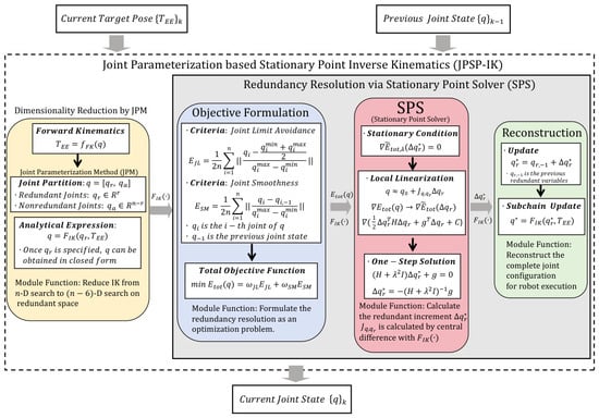
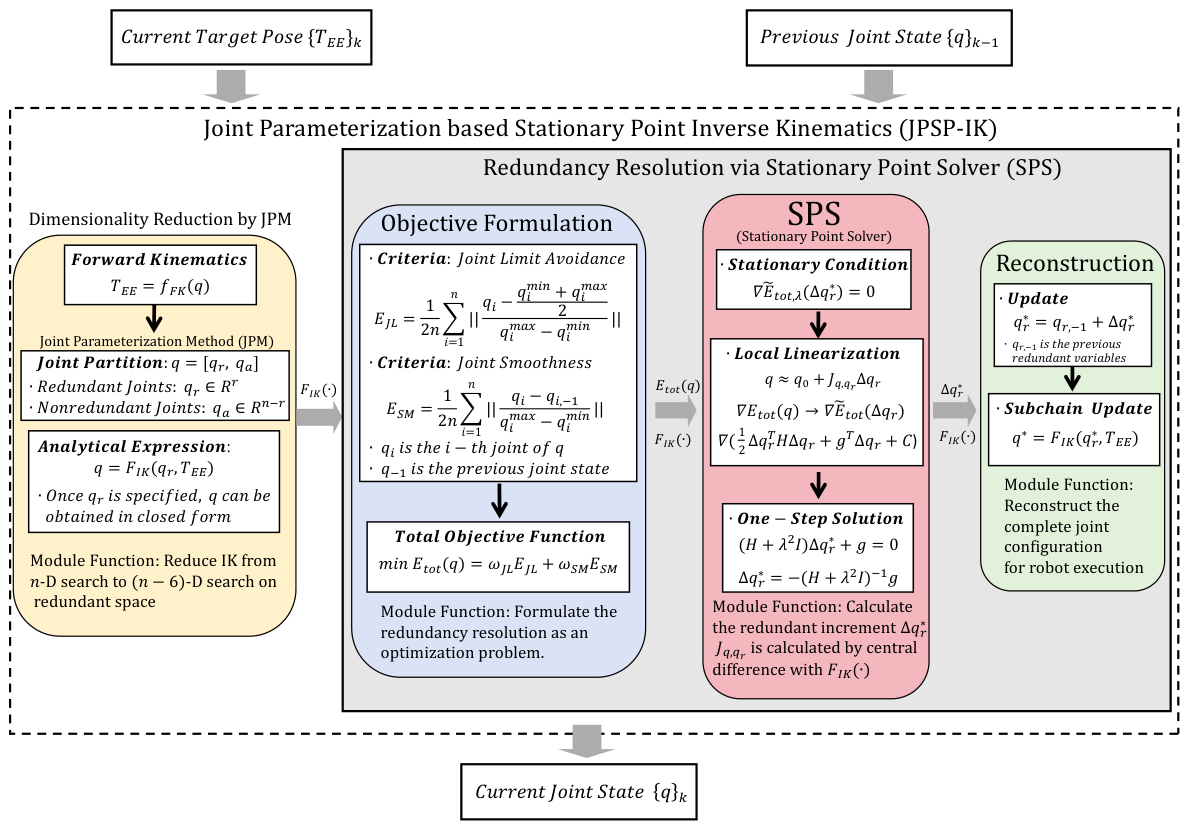
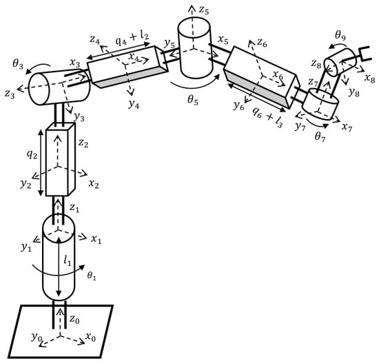
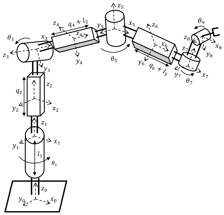
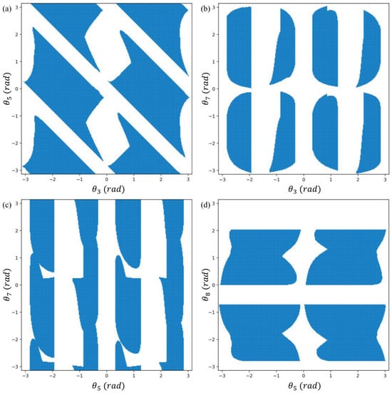
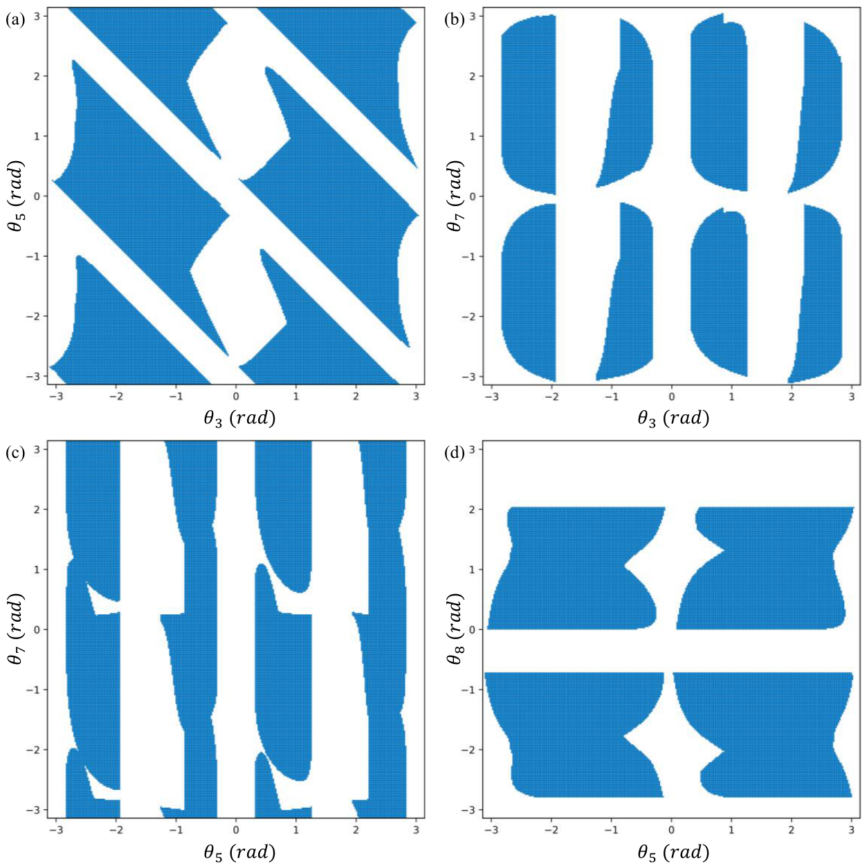
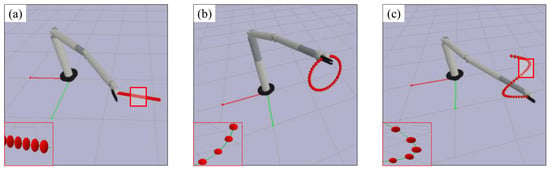
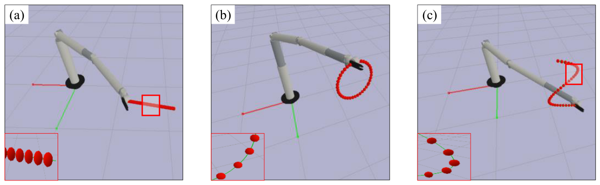
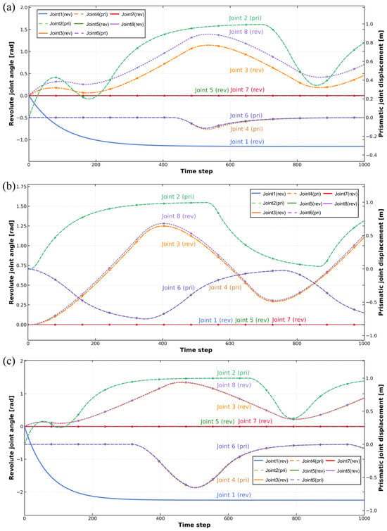
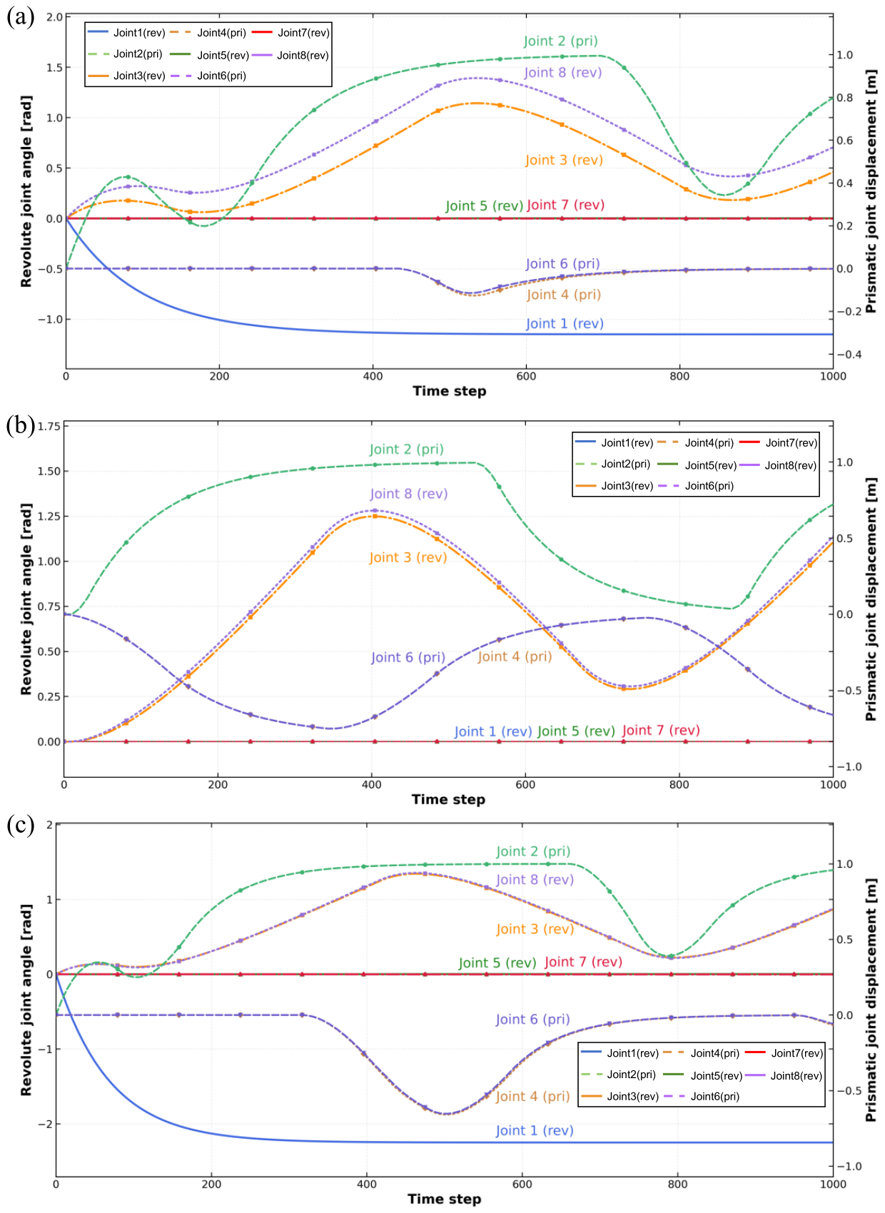
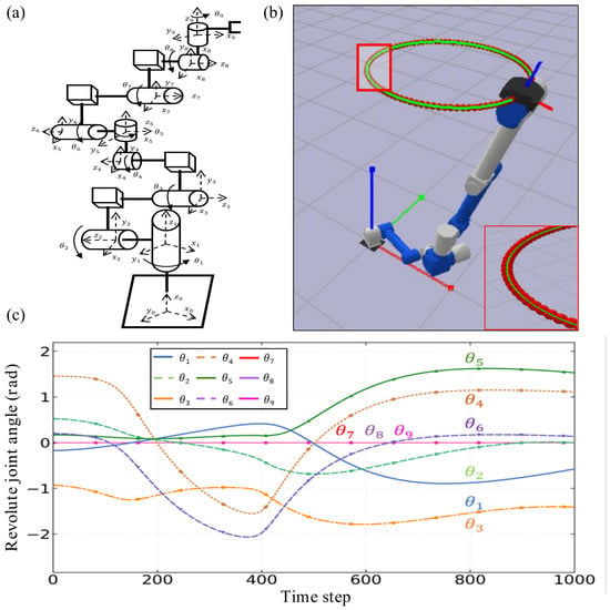
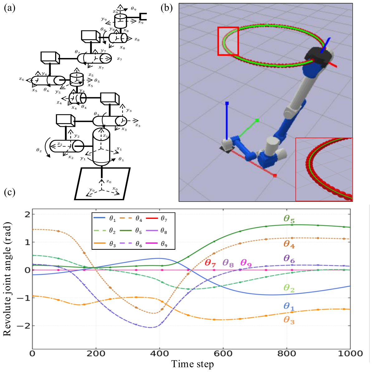
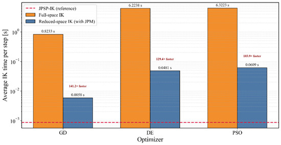
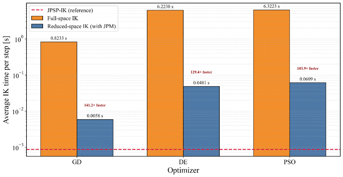
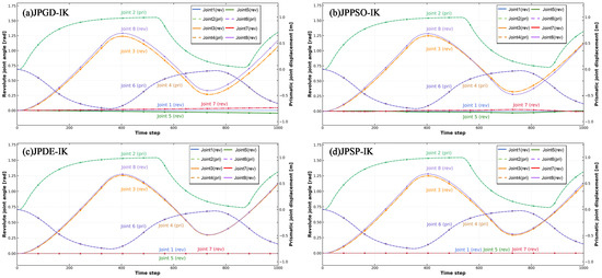
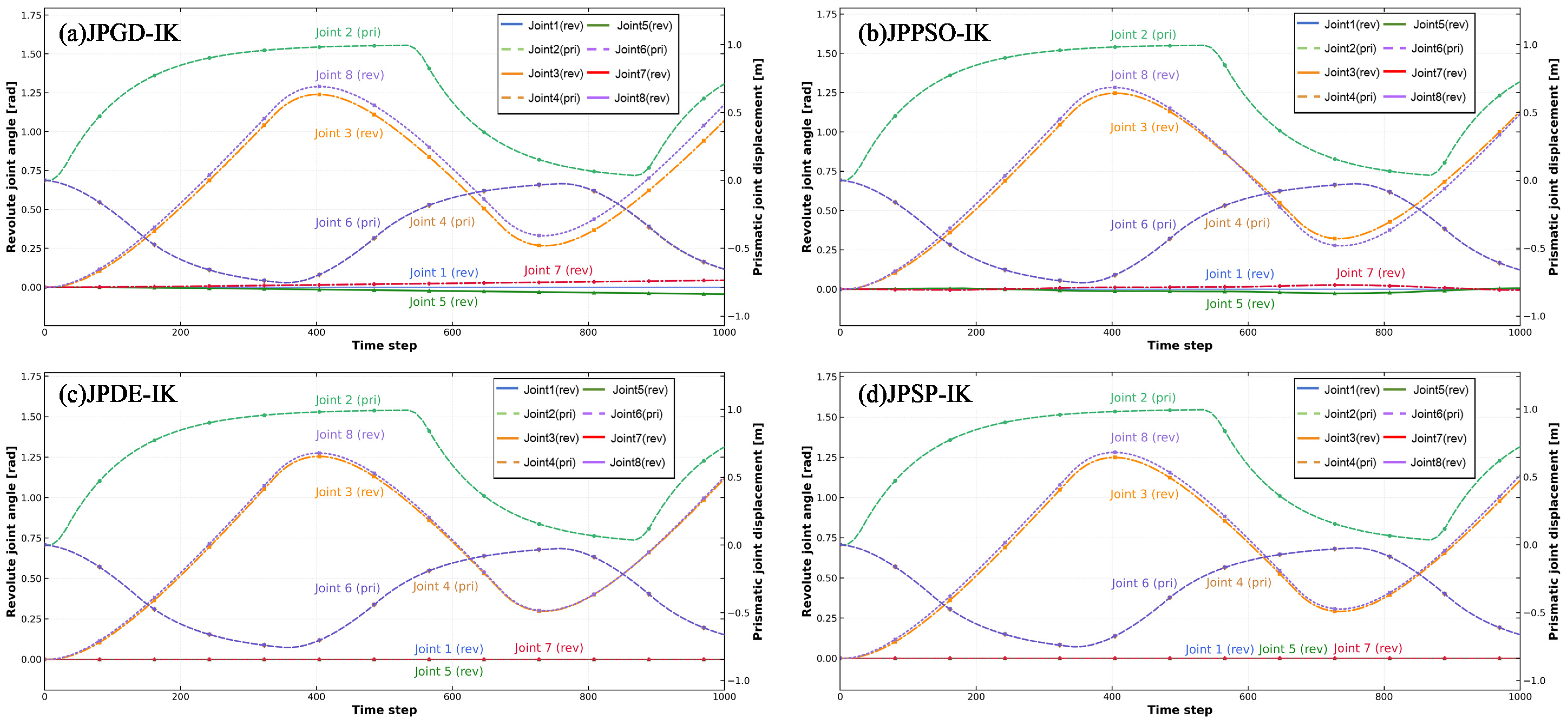
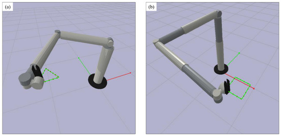
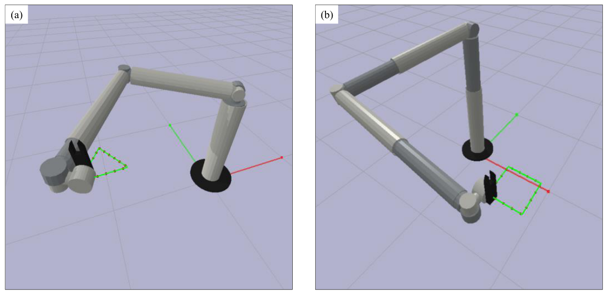
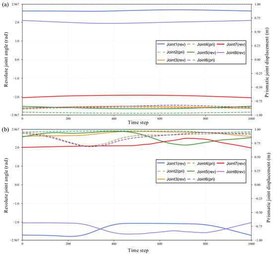
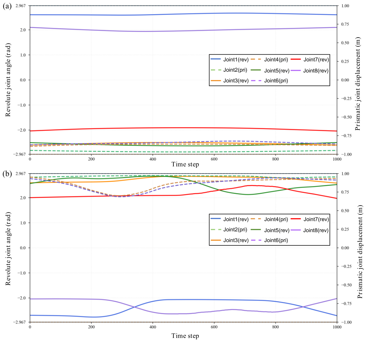
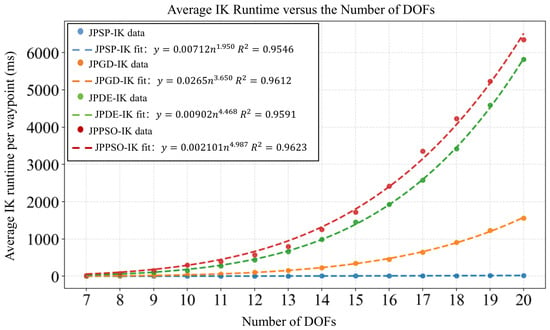
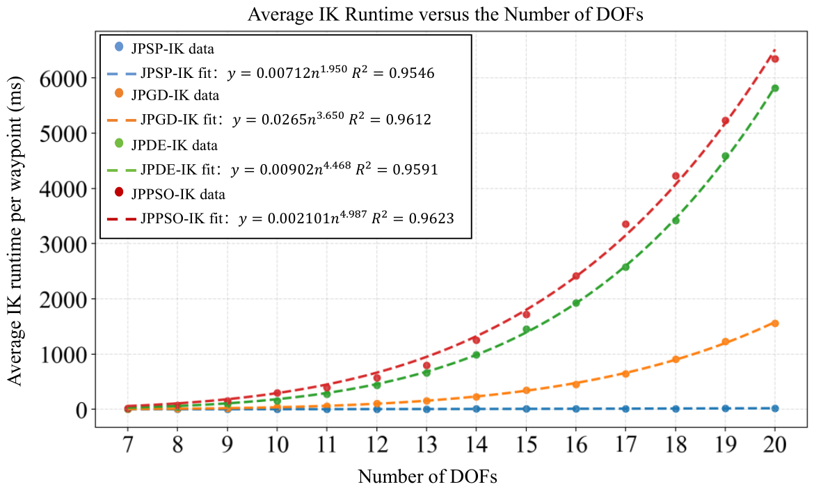

Disclaimer/Publisher’s Note: The statements, opinions and data contained in all publications are solely those of the individual author(s) and contributor(s) and not of MDPI and/or the editor(s). MDPI and/or the editor(s) disclaim responsibility for any injury to people or property resulting from any ideas, methods, instructions or products referred to in the content. |
© 2026 by the authors. Licensee MDPI, Basel, Switzerland. This article is an open access article distributed under the terms and conditions of the Creative Commons Attribution (CC BY) license.