


Abstract
Federated learning (FL) enables privacy-preserving fault diagnosis across distributed industrial devices, but most existing methods assume homogeneous model architectures and comparable client resources. This assumption is unrealistic in resource-constrained Industrial Internet of Things (IIoT) scenarios, where clients may have substantially different memory and computation capacities. To address this challenge, we propose FedAnchor, an anchored and adaptive FL framework for resource-heterogeneous fault diagnosis. FedAnchor decomposes each client submodel into a shared anchored core and a client-specific adaptive extension. The anchored core provides a common parameter subspace for consistent masked aggregation, while the adaptive extension is selected by a server-side reinforcement-guided policy under client memory budgets. This design couples resource-aware submodel allocation with structurally aligned aggregation. Experiments on four benchmark datasets and six heterogeneous memory configurations show that FedAnchor achieves competitive or superior accuracy compared with representative homogeneous and model-heterogeneous FL baselines. Under the evaluated non-IID settings, FedAnchor improves accuracy by up to 9.8 percentage points over the strongest baseline, while maintaining favorable communication–accuracy trade-offs and empirical stability.
1. Introduction
Rotating machinery, such as bearings, motors, and gearboxes, plays a critical role in modern industrial systems. Failures can cause costly downtime and safety risks, making accurate fault diagnosis essential. Deep learning (DL) has achieved strong diagnostic performance by learning discriminative patterns from vibration and acoustic signals [1,2,3,4]. However, accurate models usually require large and diverse labeled datasets, which are rarely available at a single site. In addition, privacy regulations (e.g., GDPR [5]) and network limitations often prevent raw industrial data from being shared across factories or organizations. Federated learning (FL) addresses this issue by allowing clients to train a shared model collaboratively while keeping raw data local [6,7,8].
A major challenge in federated fault diagnosis is client-side resource heterogeneity. Edge devices may differ substantially in memory capacity and computational power. Excluding weak clients can introduce participation bias, whereas uniformly shrinking the model underutilizes high-resource devices [9,10]. A more flexible solution is to let clients train resource-feasible submodels. However, this introduces structural mismatches: Different clients update different parameter subsets, and naive aggregation may average parameters with inconsistent update histories. Therefore, a resource-adaptive FL method must not only assign feasible submodels but also preserve a shared aggregation structure.
Knowledge-distillation-based methods [11,12,13] can align heterogeneous models, but they often assume a shared public dataset or require exchanging intermediate representations. Existing submodel-based methods usually rely on random dropout, fixed width scaling, or cyclic activation of model components [14,15,16]. These strategies reduce local resource usage, but they do not explicitly separate a shared aggregation subspace from a client-specific adaptive subspace. As a result, resource adaptation and aggregation consistency are often handled separately or implicitly.
To address these challenges, we propose FedAnchor, an anchored and adaptive federated learning framework for resource-heterogeneous fault diagnosis. FedAnchor decomposes each client submodel into a small anchored core shared by all clients and a client-specific adaptive extension. The anchored core provides a common parameter subspace for consistent masked aggregation, while the adaptive extension is selected by a server-side deep reinforcement learning policy according to client memory budgets and training feedback. This design couples resource-aware submodel allocation with structurally aligned aggregation in a unified framework.
As illustrated in Figure 1, conventional homogeneous FL relies on one full model for all clients, which is often unsuitable for resource-heterogeneous IIoT devices. FedAnchor addresses this mismatch by assigning different submodels according to client memory budgets while retaining a shared anchored core for aggregation alignment. The server-side selector determines the submodel structure, whereas clients only train their assigned submodels. This design highlights the central idea of FedAnchor: data-driven, resource-aware submodel coordination with a shared anchored subspace for more consistent aggregation under heterogeneous client resources. Different from random or fixed submodel pruning, the parameters used for cross-client aggregation are explicitly protected by the anchored core, whereas the remaining extension is adapted to client-specific budgets.
Figure 1.
Motivation and overview of FedAnchor under resource heterogeneity. (a) Conventional homogeneous FL requires every client to train the same full global model, which may cause memory overflow, high communication cost, or participant dropout when client resources differ. (b) FedAnchor uses a server-side selector to assign resource-aware submodels while preserving a shared anchored core for masked aggregation over a common parameter subspace. Dark blue blocks denote the anchored core shared across clients, and light blue blocks denote client-specific adaptive extensions.
Our main contributions are summarized as follows:
- We formalize federated fault diagnosis under multi-tiered memory constraints, where clients may train structurally different submodels while raw industrial data remain local. This formulation bridges the gap between homogeneous FL assumptions and resource-heterogeneous IIoT fault diagnosis scenarios.
- We propose FedAnchor, an anchored and adaptive FL framework for structurally heterogeneous clients. Unlike homogeneous FedAvg-style training, dropout-based submodel training, or fixed nested submodels, FedAnchor decomposes each client submodel into a shared anchored core and a client-specific adaptive extension. The anchored core supports consistent masked aggregation, while the adaptive extension is selected by a server-side reinforcement-guided policy under client memory budgets. Section 4 further decomposes the roles of reinforcement-guided allocation, anchored alignment, and masked aggregation.
- We conduct experiments on four public fault diagnosis datasets, namely CWRU, JNU, XJTU, and MFPT, under six heterogeneous memory configurations and both IID and non-IID data partitions. The results show that FedAnchor achieves competitive or superior diagnostic accuracy compared with representative homogeneous and model-heterogeneous FL baselines. Additional analyses of signal-level responses, feature-shift partitions, client selection policies, convergence behavior, and raw communication volume further examine the behavior and practical trade-offs of the proposed framework.
2. Related Work
In recent years, FL has emerged as a machine learning paradigm for collaborative fault diagnosis in industrial settings, particularly for rotating machinery, where privacy-preserving and efficient model training are critical. Although FL has demonstrated substantial potential, several challenges remain in representative applications, especially in handling client heterogeneity, diverse resource constraints, and the adaptability of learning frameworks to representative industrial conditions. This section reviews recent advances in federated learning for fault diagnosis, with a particular focus on model heterogeneity and resource-adaptive strategies.
2.1. Federated Learning for Fault Diagnosis
Federated learning has attracted increasing attention as a viable framework for intelligent fault diagnosis in rotating machinery, offering a privacy-preserving solution for collaborative model training across distributed industrial devices. By enabling sensors and edge nodes to jointly train a global model without transferring raw data, FL mitigates data isolation while complying with regulatory constraints such as GDPR [6]. Recent studies have extended FL-based fault diagnosis to dynamic operational environments through techniques such as adaptive validation [7] and cross-device domain generalization [17], which improve performance under changing working conditions.
In parallel, personalized federated learning (PFL) approaches have been proposed to accommodate client-specific characteristics. For example, Kolmogorov–Arnold-enhanced convolutional neural networks have been applied to personalized rotating machinery fault diagnosis [18]. To address limited and imbalanced data distributions across clients, meta-learning [19] and transfer learning [20] have been integrated with FL to enhance generalization and client-level adaptation. Transfer-based FL frameworks, such as FTSDC [21], introduce dual-correction mechanisms for cross-machine fault scenarios, while knowledge distillation techniques facilitate heterogeneous learning across IoT systems [22]. Despite these advances, many existing FL-based fault diagnosis methods implicitly assume homogeneous model architectures and overlook practical hardware diversity, particularly in terms of memory and computational constraints. These limitations motivate the development of resource-adaptive federated learning frameworks, such as FedAnchor, which support personalized submodel construction and consistent aggregation under multi-tiered device constraints.
2.2. Federated Learning with Model Heterogeneity
Model heterogeneity across clients poses a fundamental challenge to federated learning, especially in industrial environments where devices exhibit substantial variation in memory capacity, computational power, and communication bandwidth. Traditional FL algorithms, which assume uniform model architectures, often struggle to scale effectively under such heterogeneous conditions. Federated dropout (FD) [14] addresses this issue by randomly pruning the global model to generate lightweight submodels for individual clients. However, the stochastic nature of FD can lead to less consistent training and insufficient training of shared parameters, particularly for resource-constrained devices.
To improve structural efficiency, several approaches explicitly design heterogeneous model architectures. Methods such as FjORD [23], HeteroFL [24], and Fluid [15] allocate fixed substructures according to predefined client resource profiles. While these approaches improve parameter utilization, they lack adaptability to dynamic changes in client capabilities and cannot adjust model structures as training progresses. More flexible strategies, including FedRolex [16], employ rolling submodel activation across communication rounds to enhance allocation diversity. Adaptive federated dropout [25] further introduces structure–performance tables to guide submodel reuse, albeit at the cost of increased convergence latency. Successive layer training (SLT) [26] incrementally expands a model’s depth, enabling progressive learning from shallow to deeper networks for constrained devices, but it remains limited in lateral scalability and sensitivity to task heterogeneity.
Recent hypernetwork-based approaches provide another direction for personalized and model-heterogeneous federated learning. Shamsian et al. proposed personalized Federated HyperNetworks (pFedHN), where a server-side hypernetwork generates personalized model parameters for different clients, enabling parameter sharing while maintaining client-specific models [27]. Litany et al. further studied federated learning with heterogeneous architectures using graph hypernetworks, where client architectures are represented and processed through a graph-based hypernetwork to support parameter generation across different model structures [28]. These methods are highly relevant to model heterogeneity because they allow client models to differ in architecture or parameterization. However, their system’s assumptions differ from the submodel-coordination setting considered in this work. Hypernetwork-based methods usually introduce an additional model generator on the server and aim to produce personalized client models, whereas FedAnchor maintains a single global diagnostic model and extracts resource-feasible submodels from a shared parameter space.
In addition, personalized federated learning has also been investigated in natural language processing scenarios. For example, Wang et al. studied personalized federated text classification with gradient-free prompt tuning, where personalization is achieved through prompt-level adaptation for language models [29]. Such NLP-oriented personalized FL methods broaden the application scope of federated learning, but they are not directly comparable to the present vibration-signal fault diagnosis setting because their data modality, backbone model, task objective, and personalization mechanism are designed for text classification rather than 1D vibration-based industrial diagnosis. Therefore, these methods are discussed as relevant personalized or heterogeneous FL studies, while the experimental comparison in this work focuses on submodel-based baselines that can be directly adapted to resource-constrained fault diagnosis.
Recent Resource-Adaptive and Model-Heterogeneous FL Methods: Recent studies have further investigated resource-adaptive and model-heterogeneous FL under system-heterogeneous clients. NeFL introduces nested model scaling for clients with heterogeneous system resources and analyzes the inconsistency caused by training multiple submodel architectures [30]. FIARSE proposes Federated Importance-Aware Submodel Extraction, which dynamically adjusts client submodels according to parameter importance for model-heterogeneous FL with clients of different computational capacities [31]. These studies are closely related to the present work because they also address resource-aware model adaptation. However, their mechanisms differ from FedAnchor: NeFL follows the nested submodel-scaling family, while FIARSE focuses on importance-aware extraction. In contrast, FedAnchor explicitly couples a shared anchored aggregation subspace with a client-specific adaptive extension. This design aims to maintain aggregation consistency while still exploiting heterogeneous client memory budgets.
Although these recent methods are highly relevant, not all of them are directly comparable under the experimental protocol of this paper. Our direct baselines are selected to use the same 1D-CNN backbone, the same synchronous partial-participation FL protocol, the same train/test splits, and the same memory-tier settings. Under this criterion, the comparison already includes SLT, a recent resource-constrained submodel-training method, together with HeteroFL and FedRolex as representative nested and rolling submodel baselines. Recent methods such as NeFL and FIARSE are therefore discussed to clarify the latest research landscape and the relationship between FedAnchor and recent resource-adaptive FL, while the direct experiments are kept under a unified implementation protocol for fair comparison. The key characteristics of these methods are summarized in Table 1.
Table 1.
Qualitative positioning of FedAnchor against representative heterogeneous and personalized federated learning methods.
Other approaches, such as selective knowledge distillation [22] and cross-domain collaborative updates [17], provide partial flexibility in heterogeneous settings but often rely on additional data assumptions or implicit architectural compatibility. Overall, existing methods either lack fine-grained adaptivity, incur additional communication or coordination overhead, or fail to explicitly promote aggregation consistency under structural diversity. In contrast, FedAnchor addresses these limitations by combining server-side adaptive submodel allocation with an anchored aggregation mechanism, enabling resource-aware federated learning under multi-tiered resource heterogeneity.
3. Problem Statement
- Notation: To facilitate understanding of the proposed framework, the main symbols used throughout this paper are summarized in Table 2. These symbols are formally introduced in subsequent sections but are listed here for clarity and quick reference.
Table 2.
List of main symbols used in this work.
- System Setup: Modern industrial systems, such as wind farms and smart factories, deploy distributed sensors and edge devices to monitor rotating machinery in resource-constrained Industrial IoT environments. Such systems typically consist of a heterogeneous mix of low-power edge nodes and high-performance servers, forming a federated and resource-diverse network. Each device collects local vibration or acoustic signals, while raw data sharing across sites is restricted due to privacy regulations and communication limitations.
We consider a federated learning system comprising K clients indexed by . Each client k owns a local dataset , where and denote the input signal and corresponding fault label, respectively. Client k is subject to a normalized memory budget , which specifies the maximum scalable training–memory proportion of the global model that can be allocated to the client-side submodel. We use as a resource-capacity constraint rather than a raw parameter-count constraint. During local training, the peak memory consumption of a submodel includes not only model weights but also gradients, optimizer states, intermediate activations, and the local minibatch buffer. Therefore, the memory budget is interpreted through an estimated training–memory model rather than by parameter count alone. To reflect representative IIoT resource conditions, we consider multi-tiered resource heterogeneity, e.g., , which captures a spectrum of devices ranging from embedded edge nodes to GPU-accelerated servers.
For a submodel trained with minibatch size b, its estimated peak training memory can be written as
where , , and denote the memory occupied by model weights, gradients, and optimizer states, respectively. denotes the memory required to store intermediate activations for back-propagation, is the input minibatch buffer, and denotes framework-dependent temporary buffers. The memory components considered in this work are summarized in Table 3.
Table 3.
Training–memory components considered in the memory-budget model.
Let be the number of trainable parameters in , and let q be the number of bytes per floating-point value. In our implementation of FP32 with training and SGD with momentum, the parameter-related memory is approximated as
where for SGD with momentum because one additional momentum buffer is maintained. The activation memory is estimated from the feature-map sizes of the selected submodel:
where denotes the number of activation elements retained at layer ℓ of submodel . For the 1D-CNN used in this work, is determined by the temporal length and channel width of the corresponding layer. The local minibatch buffer is fixed across methods because all experiments use the same input window length and minibatch size. Accordingly, the client memory constraint is enforced on the scalable part of the training memory:
The fixed minibatch buffer and framework-dependent buffers are included when discussing actual device memory, but they are not used to differentiate methods because they are kept identical across all compared approaches. Thus, should be understood as a normalized scalable training–memory budget that controls the size of the client-side trainable submodel.
The global objective is to collaboratively train a fault diagnosis model under strict privacy constraints such that raw data never leaves local clients. Due to heterogeneous resource budgets, each client trains a personalized submodel that satisfies its memory constraint . The federated system must therefore allow updates from structurally heterogeneous submodels to be aggregated in a consistent manner while maintaining diagnostic performance across clients.
- Practical Challenges: This setup introduces three key challenges.
First, enforcing a uniform global model across clients with diverse memory and computational capacities is impractical. Naively truncating layers or filters to fit resource-limited devices may discard diagnostically critical components, such as fault-induced impulses or high-frequency modulations, which are relevant for fault localization. Such indiscriminate pruning can reduce diagnostic performance in practical industrial scenarios.
Second, heterogeneous clients train structurally different submodels, which leads to structural misalignment during model aggregation. In this case, parameters with the same index across different submodels may correspond to different update histories or functional roles. Directly averaging such heterogeneous updates can result in invalid aggregation, less consistent training, and degraded global performance, particularly under non-IID data distributions.
Third, many existing approaches rely on static pruning strategies or heuristic dropout mechanisms that fail to adapt to evolving training dynamics. These methods cannot fully exploit device-specific capabilities or respond effectively to changing optimization states, limiting their applicability in dynamic and resource-constrained industrial environments.
Therefore, an effective federated learning framework must jointly support adaptive submodel construction under client-specific resource constraints and promote aggregation consistency and reduce empirical training variability across structurally heterogeneous models.
- Learning Objective: The federated optimization objective is formulated aswhere denotes a supervised loss function (e.g., cross-entropy), and is the total data size. This objective captures the weighted empirical risk across clients, subject to two constraints: (i) Each client k trains a submodel that satisfies its memory budget , and (ii) data privacy is preserved by exchanging only model parameters rather than raw data. The global model must therefore learn effectively from heterogeneous submodels under these constraints.
- Constrained Resource-Heterogeneous FL formulation: To make the resource-aware learning problem explicit, let denote the parameter vector of the global model at communication round t. For client k, the executable submodel is represented by a binary mask , and the corresponding local trainable parameter vector isThe resource-heterogeneous federated diagnosis problem can then be written as the following mask-constrained empirical-risk minimization problem:subject towhere denotes the anchored mask shared by all clients, and ⪯ indicates element-wise inclusion. Equation (8) enforces client-specific scalable-memory feasibility, while Equation (9) ensures that every client submodel contains the same anchored parameter subset for aggregation alignment. This formulation makes explicit that FedAnchor jointly addresses resource feasibility, submodel heterogeneity, and anchored aggregation consistency.
4. Methodology
FedAnchor connects the problem formulation in Section 3 with a practical learning pipeline for resource-heterogeneous federated fault diagnosis. It contains three interacting components: a server-side reinforcement-guided submodel selector, an anchored alignment mechanism, and a masked aggregation scheme. The selector allocates adaptive capacity within each client’s feasible memory budget. The anchoring mechanism defines a fixed shared parameter subset that every client submodel must retain. Masked aggregation then aggregates valid parameters from heterogeneous submodels while applying FedAvg-like updates on the anchored subspace, as illustrated in Figure 2.
Figure 2.
Overall architecture of FedAnchor. The pipeline includes federated state observation, action generation by the server-side actor network, resource-feasible submodel allocation, local training, masked aggregation, replay-buffer storage, and actor–critic policy updates.
- Summary of the Proposed Method: The proposed method is FedAnchor, an anchored and adaptive federated learning framework for resource-heterogeneous fault diagnosis. It consists of three core designs. First, a resource-feasible submodel construction mechanism maps each client’s memory budget to an executable submodel. Second, a server-side reinforcement-guided selector learns where to place the client-specific adaptive extension within the feasible submodel space. Third, an anchored core is deterministically retained by all clients, and masked aggregation updates this shared subspace consistently across heterogeneous submodels. Therefore, FedAnchor is not a new optimizer or a replacement for the FL communication protocol. Instead, it is a resource-aware submodel coordination strategy that extends FL to clients with heterogeneous memory budgets.
- Unified Mathematical Formulation of FedAnchor: FedAnchor constructs each client mask as a union of two disjoint components:where is the deterministic anchored mask shared by all clients, is the client-specific adaptive mask selected under memory budget , and ∨ denotes element-wise logical OR. The two masks satisfywhich prevents overlap between anchored and adaptive parameters. The adaptive mask is generated by a server-side policy and a feasibility projection:where is the actor policy, is the server-side state, maps the policy action to layer-wise adaptive candidate indices, and enforces the client-specific memory constraint. The final submodel sent to client k is thereforeThis unified formulation links the resource-feasible projection, reinforcement-guided adaptive selection, anchored core preservation, and masked aggregation in a single mask-based mathematical model. The main differences from representative resource-heterogeneous federated learning approaches are summarized in Table 4.
Table 4.
Comparison between FedAnchor and typical federated learning approaches under resource-heterogeneous settings.
- Module-Level Contribution Decomposition: To clarify the boundary between reinforcement-guided allocation and anchoring, Table 5 summarizes the role and dependency of each module. DRL is responsible for adaptive capacity allocation, while anchoring defines the shared aggregation subspace. Their main interaction occurs in boundary-aware submodel construction, where the DRL-selected adaptive extension is placed outside the fixed anchored subset under the client-specific memory constraint. Masked aggregation then uses the resulting masks to aggregate heterogeneous submodel updates consistently.
Table 5.
Module-level contribution decomposition and dependency analysis of FedAnchor.
4.1. Reinforcement-Guided Submodel Extraction
Client devices in federated networks exhibit substantial heterogeneity in memory budgets , where . To respect these constraints, each client trains a partial submodel of the global model such that . Because submodel structure selection affects not only immediate performance but also future aggregation behavior, we formulate submodel allocation as a sequential decision-making problem. Accordingly, we model this process as a Markov decision process (MDP) and adopt the Deep Deterministic Policy Gradient (DDPG) algorithm [32] to learn a continuous, resource-aware allocation policy. The DDPG agent is maintained and updated on the server side, where sufficient computational and memory resources are assumed to be available. Resource-constrained clients do not execute the actor–critic networks, maintain replay buffers, or perform policy updates; they only receive the selected submodel structure or mask for local training. Therefore, using DRL for allocation does not contradict the resource-constrained client setting, because the additional decision-making overhead is centralized at the server.
- State Representation: The system state at communication round t is defined aswhere denotes the aggregated client-reported feedback accuracy from the previous communication round; , , and are the three components of the previous layer-wise action vector corresponding to Conv1, Conv2, and the fully connected layer, respectively; represents normalized training progress. Therefore, the state dimension is five, consisting of one scalar feedback-performance indicator, three historical allocation indicators, and one training-progress indicator.
Feedback accuracy is collected without introducing an additional public validation dataset or exchanging raw samples, logits, or intermediate features. At the end of each communication round, each selected client reports only a scalar local feedback accuracy value computed during its local training/evaluation procedure. The server aggregates these scalar reports as
where is the set of clients selected in round , is the number of local training samples on client k, and is the scalar feedback accuracy reported by client k. This feedback signal is used only for server-side policy learning and is not used as the final test metric. Final diagnostic performance is evaluated separately on the held-out test set described in Section 5. This state formulation captures current feedback performance, historical allocation context, and training progress, enabling temporally informed allocation decisions.
- Action Space: The actor network generates a continuous action vectorwhere denotes the deterministic policy parameterized by , and is Gaussian noise added for exploration during training.
- Resource-Feasible Action Mapping: The actor output does not directly determine an unconstrained model size. Instead, it determines the layer-wise positions of adaptive neuron blocks within a client-specific feasible submodel space. For each selected client k, the action is mapped to a submodel through a resource-feasible projection:subject towhere denotes the action-guided submodel construction operator, and denotes the feasibility projection under the memory budget of client k. Therefore, the resource constraint is enforced before local training begins. The policy learns which parts of the global model should be activated within the allowed budget rather than learning to arbitrarily increase or decrease the client-side model’s size. It is important to note that the DRL policy controls only the adaptive extension of each submodel. The shared anchored subset is not selected by the policy; it is deterministically preserved to maintain a common aggregation subspace across clients.
- Reward Function: The reward at round t is defined aswhere and denote the normalized aggregated client-reported feedback accuracies of the current and previous communication rounds, respectively. The first term encourages policies that maintain a high feedback-performance level, while the second term explicitly captures incremental improvement across rounds.
We do not include an additional memory or communication penalty in the reward because resource feasibility is enforced as a hard constraint during submodel construction. For each client k, the selected submodel must satisfy the scalable memory constraint defined in Equation (4) before local training is performed. Under a fixed memory-tier configuration, the role of the policy is therefore to determine where the adaptive capacity is allocated within the feasible submodel rather than how much memory the client is allowed to use. Similarly, the communication volume of each client update is upper-bounded by the size of its feasible submodel and is evaluated separately in the communication-cost analysis. Adding a soft resource penalty to the reward would provide limited additional information under fixed memory budgets and could bias the policy toward overly small or under-trained submodels.
Therefore, FedAnchor implements resource awareness through constrained submodel feasibility and client-specific memory budgets, while the reward focuses on learning diagnostically effective allocations within those budgets. Since this feedback is computed locally and reported only as scalar values, it does not require a separate public validation dataset or any exchange of raw data, logits, or intermediate representations. The feedback signal is used only to guide the server-side allocation policy, whereas the final diagnostic accuracy is reported on the held-out test set. This composite reward design uses a learning signal that reflects both long-term performance levels and short-term optimization dynamics for temporally coupled submodel allocation decisions in federated training.
This reinforcement-guided module establishes the foundation for adaptive and resource-aware submodel selection. However, to promote consistent aggregation across heterogeneous submodels, additional structural constraints are required. We address this challenge through an anchor-based submodel construction, which is described next.
4.2. Anchored Submodel Construction
Although the DRL agent dynamically selects personalized neuron blocks for each client, unconstrained submodel extraction may remove parameters that are repeatedly updated across clients, which can lead to aggregation variability under structural heterogeneity. To address this issue, we introduce an anchored submodel construction strategy that explicitly preserves a small, shared parameter subset across all clients, thereby enforcing a consistent update subspace during federated aggregation.
Specifically, for each layer ℓ, we reserve a proportion of neurons as anchor parameters, where denotes the memory constraint of client k. Anchors are implemented as a fixed index set consisting of the first neurons in layer ℓ, where is the total number of neurons. This design serves as a deterministic coordination mechanism that preserves identical parameter subsets across heterogeneous clients, without introducing additional communication, data exchange, or feature-level matching. The anchoring mechanism is therefore not responsible for learning the client-specific allocation policy. Its role is to define a stable structural constraint that every policy-generated submodel must satisfy.
The anchoring ratio is treated as a structural design parameter that controls the size of the shared update subspace. Rather than assuming semantic correspondence at the feature level, the anchors are intended to maintain a statistically consistent and repeatedly updated parameter subset across clients. In practice, we set as a default value, which provides a measured balance between aggregation consistency and personalized model capacity under diverse resource configurations. Importantly, this choice does not affect the generality of the framework and can be adjusted to accommodate different resource constraints or application requirements.
Signal-level interpretation of anchored parameters. It should be noted that the anchored neurons are not pre-assigned to manually defined physical frequency bands. In a 1D-CNN-based diagnostic model, convolutional channels act as learnable temporal filters, and their frequency responses emerge from data-driven training rather than from fixed signal-processing rules. Therefore, FedAnchor does not assume a one-to-one correspondence between an anchored neuron and a specific bearing characteristic frequency, such as BPFO, BPFI, or BSF, or a manually defined spectral band.
Instead, the purpose of anchoring is to ensure that a small subset of learnable filters is retained and repeatedly updated by all participating clients during federated aggregation. This shared update exposure encourages the anchored channels to capture diagnostic patterns that are more stable across clients, such as fault-induced impulses, periodic modulation, and broadband or high-frequency vibration components that commonly appear in bearing fault signals. Meanwhile, the non-anchored adaptive channels can still model client-specific operating conditions, load variations, and local data distributions. The anchored subspace is therefore not intended to encode fixed physical features but to preserve a commonly updated diagnostic representation that stabilizes aggregation under structural heterogeneity without requiring explicit feature-level alignment.
Beyond the anchored parameters, the remaining neurons are selected adaptively by the DRL agent under explicit boundary constraints. For client k and layer ℓ, we first define the layer-wise neuron budget as
where is the number of neurons or channels in layer ℓ. The number of anchored neurons is defined as
and the number of dynamically selected neurons is
The anchor index set is fixed as
If , no dynamic neuron is selected for this layer. Otherwise, the start index of the dynamic block is computed as
where is the layer-wise action generated by the policy network. The dynamic index set is then
This construction guarantees that because , and it prevents out-of-bound selection because . The final valid neuron set is
which satisfies
Therefore, anchor preservation and adaptive selection are performed within the same client-specific layer-wise budget rather than adding dynamic neurons on top of the budget. After the layer-wise selection is completed, the resulting submodel is further checked by the scalable-memory feasibility condition in Equation (18).
Algorithm 1 summarizes the anchored submodel extraction procedure. By construction, every client submodel retains an identical anchored parameter subset while allowing flexible, resource-aware personalization through non-overlapping DRL-controlled dynamic components. This structure provides the basis for masked aggregation under heterogeneous model architectures, as detailed next.
| Algorithm 1 Anchored Submodel Extraction Guided by DRL Action with Boundary Handling |
| Require: Global model ; memory constraint ; action vector ; anchoring ratio Ensure: Customized submodel
|
4.3. Masked Aggregation with Alignment
After local training, client k uploads a masked update
where denotes the locally trained parameter vector, and inactive parameters are set to zero by . Because heterogeneous clients may activate different non-anchored parameters, aggregation should be normalized over the clients that actually update each parameter. For each parameter index j, the server computes the active weighted denominator
The global update is then performed by parameter-wise normalized masked aggregation:
This normalization ensures that a non-anchored parameter is averaged only over clients that actually train and upload that parameter, while parameters inactive for all selected clients remain unchanged.
To analyze the aggregation behavior under structural heterogeneity, we interpret Equation (30) from the perspective of a shared anchored parameter subspace. Let denote the anchored parameter subset, and let denote the non-anchored subset. Each local update can be decomposed as
The anchored subset is retained by every selected client, whereas the non-anchored adaptive subset may vary across clients and rounds.
Proposition 1.
For any anchored parameter index j satisfying , the FedAnchor update is equivalent to FedAvg restricted to the anchored subspace.
Proof.
Since the anchored mask is retained by every selected client, we have for all . Therefore,
Substituting Equation (32) into the parameter-wise masked aggregation rule gives
which is the standard FedAvg update applied to the anchored parameter j. □
Consequently, the overall FedAnchor update can be interpreted as the combination of a FedAvg-like update on the shared anchored subspace and a mask-normalized update on the non-anchored adaptive subspace:
where denotes the parameter-wise normalized update in Equation (30) restricted to the non-anchored parameters. This decomposition indicates that FedAnchor supports aggregation consistency and structural adaptability without requiring full model homogeneity or feature-level alignment. It also clarifies the interaction between modules: DRL affects which non-anchored adaptive parameters are activated, whereas anchoring guarantees that a FedAvg-like update is always performed on the shared anchored subspace.
4.4. Policy Optimization Procedure
The DDPG policy is optimized on the server side using replay-based off-policy learning. The server-side policy aims to maximize the expected discounted return
where denotes the actor parameters, and is the feedback-based reward defined in Equation (19). At each communication round t, the server observes the state and generates one global layer-wise action
where corresponds to the adaptive selection decisions for Conv1, Conv2, and the fully connected layer, respectively. This action does not directly specify an independent model size for each client. Instead, the same action is combined with each selected client’s memory budget and mapped into a client-specific feasible submodel through the boundary-aware construction in Algorithm 1. Thus, one policy action is generated per communication round, while the resulting submodels are client-specific because their feasible budgets differ.
After local training and masked aggregation, the server obtains the next state and reward . The transition tuple
is stored in the replay buffer , where is a done flag. In the finite-horizon federated training process, only at the last communication round, and otherwise. When the replay buffer contains at least B transitions, the server uniformly samples a mini-batch
For each sampled transition, the target value is computed using the target actor and target critic :
The critic network is updated by minimizing the mean-squared temporal-difference error:
The actor network is updated by maximizing the critic-estimated value of the action generated by the current policy. Equivalently, the actor loss is written as
The deterministic policy gradient used for updating the actor is
After the actor and critic updates, the target networks are updated by soft replacement:
In our implementation, the policy is updated once per communication round after the replay buffer contains at least one mini-batch of transitions. This update is performed only on the server; clients neither store replay buffers nor execute actor–critic optimization.
Having defined the policy update routines, the server-side selector, anchored submodel construction, masked aggregation, and policy update form the complete FedAnchor training pipeline.
- Mathematical Model Clarification: The formulation above separates three levels of FedAnchor. At the optimization level, FedAnchor solves a resource-constrained federated empirical-risk minimization problem. At the submodel-construction level, each client mask is decomposed into a shared anchored mask and a resource-feasible adaptive mask. At the aggregation level, parameter-wise normalized masked aggregation ensures that anchored parameters receive FedAvg-like updates from all selected clients, while non-anchored parameters are updated only by clients that activate them. This formulation clarifies how adaptive allocation and anchored aggregation are coupled mathematically.
5. Experimental Evaluation
In this section, we evaluate the proposed FedAnchor framework under representative industrial conditions for fault diagnosis in rotating machinery. The experiments are designed as reproducible benchmark-based evaluations rather than full real-factory deployment tests. We use public fault diagnosis datasets to ensure controlled comparison, while resource-heterogeneous IIoT conditions are simulated through memory-tier constraints, partial participation, non-IID partitions, feature-shift partitions, and client-selection policies. Our experiments assess the performance of FedAnchor in terms of diagnostic accuracy, training variability, and resource efficiency under these controlled resource-heterogeneous conditions. To directly reflect the three challenges in Section 3, we report diagnostic accuracy (capability), empirical training variability (aggregation behavior under structural misalignment), and communication/efficiency metrics (resource-aware learning under heterogeneous constraints). We compare FedAnchor with representative federated learning methods across several benchmark datasets and resource configurations to evaluate its effectiveness in resource-heterogeneous industrial settings.
5.1. Experimental Setup
To evaluate the proposed FedAnchor framework under representative resource-heterogeneous industrial diagnosis settings, we design a series of federated diagnostic experiments on rotating machinery. These experiments simulate heterogeneous resource environments and non-IID data partitions to assess diagnostic accuracy, variability, and efficiency under representative resource constraints.
- Compared Methods: We compare FedAnchor with five representative federated learning baselines that cover homogeneous aggregation, dropout-based submodel training, nested model-heterogeneous FL, rolling submodel activation, and progressive layer-wise training.
- FedAvg-Small is a resource-feasible adaptation of FedAvg [33]. Since standard FedAvg assumes that all clients train the same model architecture, it cannot be directly executed when clients have different memory budgets. For each heterogeneous memory configuration, all clients are assigned the largest homogeneous submodel that can be loaded by the weakest client:The global model used by FedAvg-Small is therefore a uniformly scaled submodel for which its scalable training–memory ratio does not exceed . During training, every selected client downloads, trains, and uploads this same smallest feasible model, and the server performs standard FedAvg aggregation over this homogeneous parameter space. Thus, FedAvg-Small is not a model-heterogeneous baseline; rather, it serves as a conservative homogeneous FL reference that satisfies all client resource budgets without excluding weak clients. Its limitation is that it underutilizes higher-resource clients, which motivates resource-adaptive heterogeneous methods such as FedAnchor. FederatedDropout [14] reduces memory usage via structured neuron dropout while retaining the global model format. HeteroFL [24] assigns nested submodels according to client capacity and is included as a directly relevant model-heterogeneous FL baseline. FedRolex [16] activates different submodel components cyclically to maximize parameter reuse and diversity. SLT [26] gradually increases model depth layer-by-layer, enabling execution on devices with dynamic or limited capacity. These baselines cover different types of references: FedAvg-Small represents a homogeneous resource-feasible lower-bound baseline, while FederatedDropout, HeteroFL, FedRolex, and SLT represent submodel-based or model-heterogeneous FL baselines that can operate under different client capacities. All methods are re-implemented in PyTorch 2.1.0 [34] and adapted to the same submodel training interface for fair comparison.
Rationale for Comparison: The selected baselines represent typical FL strategies under resource heterogeneity. FedAvg-Small represents a homogeneous resource-feasible reference, FederatedDropout represents dropout-based submodel training, HeteroFL represents nested width-scaled heterogeneous FL, FedRolex represents rolling submodel activation, and SLT represents progressive layer-wise training. Compared with these approaches, FedAnchor jointly considers resource-feasible adaptive allocation and aggregation consistency. The adaptive extension exploits client-specific memory budgets, while the anchored core preserves a shared update subspace for masked aggregation. Therefore, the comparison evaluates whether this coupled design improves diagnostic accuracy, empirical stability, and communication–accuracy trade-off over typical homogeneous and model-heterogeneous FL strategies.
Scope of Experimental Baselines: The direct experimental baselines are selected according to two criteria. First, the method should support submodel-level training under different client resource budgets. Second, it should be implementable using the same 1D-CNN backbone, synchronous FL protocol, client partitions, memory-tier settings, and train/test splits used in our fault-diagnosis experiments. Under these criteria, FedAvg-Small, FederatedDropout, HeteroFL, FedRolex, and SLT are used as direct baselines. Recent methods such as NeFL [30] and FIARSE [31] are discussed in the Related Work Section because they represent the latest progress in resource-adaptive and model-heterogeneous FL. They are not added as additional experimental baselines in this revision to keep the direct comparison under the same implemented protocol and to avoid changing the backbone architecture, submodel interface, or system setting.
- Datasets and Diagnostic Task Construction: We adopt four publicly available rotating machinery fault diagnosis datasets: CWRU, JNU, XJTU, and MFPT. Before federated partitioning, each dataset is first converted into a supervised multi-class diagnostic task with a fixed label definition and a held-out test split. A diagnostic class is defined according to the fault category, operating condition, or their combination, depending on the annotation format of each dataset. All raw signals are segmented into fixed-length 1024-sample windows, and each window inherits the diagnostic label of its source signal record. For each dataset, 70% of the segmented windows are used for federated training, and 30% are held out for final testing. The train/test split is performed after window segmentation and before client partitioning. Therefore, the held-out test set is never used for local client training, server-side policy feedback, federated aggregation, or client partition construction. Only the training windows are distributed to clients under the IID, Dirichlet label-skew, or feature-shift settings. This protocol ensures that all compared methods use the same diagnostic task definition, the same held-out test set, and the same client-level training partitions.
Table 6 summarizes how the diagnostic task is constructed for each dataset. The CWRU dataset [35] provides bearing fault signals under controlled motor load and speed conditions and is constructed as a 10-class diagnosis task. The JNU dataset [36] contains bearing signals collected under varying speed and load conditions and is constructed as a 12-class diagnosis task based on working-condition and fault-type combinations. The XJTU dataset [37] provides run-to-failure bearing degradation signals under multiple operating conditions and is constructed as a 15-class diagnosis task. The MFPT dataset [38] contains bearing fault data from laboratory and field-related conditions and is also constructed as a 15-class diagnosis task. Although these datasets differ in acquisition platforms and operating regimes, all of them are converted into supervised multi-class fault diagnosis tasks using the same segmentation, train/test split, and federated partition protocol. Table 7 summarizes the dataset statistics and federated diagnostic task construction.
Table 6.
Diagnostic task construction for each dataset before federated partitioning.
Table 7.
Dataset statistics and federated diagnostic task construction. The diagnostic labels are defined before federated partitioning. The numbers of windows are counted after 1024-sample segmentation, and the train/test split is applied before distributing training windows to clients.
- Benchmark Scope and Application Relevance: The four public datasets used in this work are representative rotating-machinery fault diagnosis benchmarks. They provide controlled vibration-signal labels and allow reproducible comparison across different federated learning methods. We acknowledge that these datasets are smaller than full industrial IIoT deployments and cannot fully capture all practical factors, such as continuous streaming data, intermittent connectivity, device failures, asynchronous availability, and factory-scale client populations. The purpose of using these benchmarks is therefore not to claim a complete real-factory deployment but to evaluate the diagnostic and aggregation behavior of different FL methods under controlled and repeatable fault-diagnosis tasks. To better reflect the computing-resource coordination scenario targeted by FedAnchor, we simulate heterogeneous client resources through six multi-tier memory configurations, deterministic client-to-tier assignments, partial client participation, IID and non-IID data partitions, feature-shift partitions, and client-selection policy variations. These settings allow us to examine whether FedAnchor can assign feasible submodels to clients with different resource budgets and maintain structurally consistent aggregation under representative resource-heterogeneous conditions.
Federated Data Partition Protocol: For each dataset, the segmented training windows are distributed to clients. Under the IID setting, samples from each diagnostic class are uniformly and stratifiedly assigned to clients so that each client has approximately the same class distribution as the global training set. Under the non-IID setting, we use label-skew partitioning based on a Dirichlet distribution with concentration parameter . To make the non-IID split reproducible, the random seeds for the three independent runs are fixed as . For each seed, the non-IID split is generated by a class-wise Dirichlet allocation algorithm. For each diagnostic class c, all training windows belonging to class c are first shuffled using the specified seed. The client allocation proportions are then sampled as
and samples of class c are assigned to clients according to . After all classes are allocated, the client sample counts are checked to avoid degenerate clients. Specifically, each client is required to contain at least training windows; otherwise, the partition is regenerated using the same seed sequence until the minimum-sample condition is satisfied. A smaller indicates stronger label skew across clients. For each dataset, memory configuration, and seed, the generated client partitions are reused by all compared methods to ensure fair comparison. The detailed Dirichlet allocation algorithm, feature-shift partition protocol, and client-level distribution diagnostics are provided in Appendix A.1. This keeps the main experimental setup concise while preserving full reproducibility details.
- Resource Constraint Settings: To emulate resource heterogeneity across clients, we assign each client k a normalized memory budget , indicating the maximum scalable training–memory ratio of the client submodel relative to the full global model , as defined in Equation (4). Six heterogeneous memory configurations are explored. Four are three-tiered configurations: , , , and . Two are four-tiered configurations: and . These cases reflect representative resource scenarios ranging from low-computing-power edge devices to industrial server nodes. Each submodel is constructed by selecting layer-wise channels or neurons under the client-specific budget .
For reproducibility, the client-to-tier assignment is deterministic and fixed for each memory configuration, as summarized in Table 8. For three-tier configurations, the 20 clients are divided as evenly as possible into groups of seven, seven, and six clients. For four-tier configurations, clients are evenly divided into four groups of five clients. The same client identities, local data partitions, local data sizes, and random seeds are reused for all compared methods under the same dataset, memory configuration, and IID/non-IID setting. Thus, differences among methods are attributable to the learning and aggregation strategies rather than to different client assignments or data splits.
Table 8.
Client assignment for each heterogeneous memory configuration.
Fairness and Seed Control: For each dataset and each IID/non-IID setting, the client data partition is generated once per random seed and then shared by all compared methods. The client IDs are also kept fixed when assigning memory tiers, so a client with a given local dataset keeps the same memory budget within a memory configuration across all methods. The same random seeds are used for data partitioning, client sampling, model initialization, and local training schedules whenever applicable. The client sampling sequence is generated once per seed and reused by all compared methods. This protocol ensures that methods are evaluated under identical client identities, local sample sizes, class distributions, resource budgets, and participation sequences.
Memory-Budget Implementation: In the experiments, each memory tier is implemented by constraining the scalable training memory of the client submodel rather than by parameter count alone. Since all methods use the same input window length, minibatch size, optimizer, and local training schedule, the input minibatch buffer and framework-level temporary buffers are shared across methods and do not affect relative comparisons. For each candidate submodel, the layer-wise channel or neuron selection determines both the number of trainable parameters and the number of activation elements, which are then used to estimate the scalable training–memory ratio. A submodel is considered feasible for client k only if its estimated scalable training–memory ratio does not exceed . This design allows the memory tiers to approximate practical resource differences among edge devices while maintaining a reproducible and method-independent constraint protocol. It should be noted that the DDPG reward is not designed to minimize communication volume beyond the predefined client memory budgets. Instead, memory and communication efficiency are controlled by the client-specific feasible submodel constraints, while raw communication volume is reported as an independent evaluation metric.
- Implementation Details: All experiments are run on an Intel Xeon E5-2678 v3 CPU and an NVIDIA RTX 3090 GPU. We simulate clients, with clients selected per communication round unless otherwise specified. Client Selection Protocol: In the main experiments, each communication round selects out of clients uniformly at random without replacement. This setting follows the common partial-participation protocol in federated learning and simulates practical IIoT scenarios where only a subset of edge devices may be available in each round due to communication, energy, or scheduling constraints. To ensure fairness, the random client-sampling sequence is generated once per seed and reused by all compared methods, so different methods are evaluated under the same participation sequence. In resource-heterogeneous settings, random selection may induce round-wise variation in the distribution of selected memory tiers. We therefore further evaluate alternative client selection policies in Appendix A.4. The main experiments retain random selection because it is method-independent, does not rely on privileged resource scheduling, and provides a neutral baseline for comparing learning and aggregation strategies under partial participation. The base diagnostic model is a compact 1D-CNN with two convolutional blocks and one fully connected head and equipped with ReLU activations and BatchNorm. Concretely, the feature extractor consists of Conv1d(, stride , padding ) → BN → ReLU → MaxPool1d(, stride ), followed by Conv1d(, stride , padding ) → BN → ReLU → MaxPool1d(, stride ). Channel widths are scaled by the client-specific subset factor sf: the first and second conv layers output and channels, respectively. Given an input window of length 1024, the temporal dimension evolves as , so the classifier receives features after flattening. The classifier head uses FC() → ReLU → FC(#classes). Input sequences are segmented into fixed-length 1024-sample windows; we apply per-client mean–std normalization on the training split (statistics frozen at test time) and light time-domain augmentations (Gaussian perturbation and random scaling) during training only. Non-IID settings are introduced via Dirichlet sampling with concentration parameter to simulate skewed label distributions. A DDPG agent guides submodel structure by mapping global training context to pruning decisions, while anchor neurons promote aggregation consistency across heterogeneous models. For server-side policy learning, the DDPG agent uses only scalar feedback accuracies reported by the selected clients after local training. No public validation dataset is introduced for policy feedback. These feedback values are used solely for policy optimization and are separated from the final test accuracy reported in the experimental results.
- Evaluation Metrics: We report four evaluation metrics. Accuracy measures classification performance on unseen test data. Training loss reflects optimization behavior.
Raw communication volume records the total bidirectional traffic during training, including both server-to-client downloads and client-to-server uploads.
Communication and Runtime Accounting: To make the resource-efficiency analysis transparent, we report the raw communication volume, the number of transmitted parameters, and the wall-clock training time for each method. Raw communication volume is defined as the total bidirectional serialized traffic between the server and the selected clients, including both server-to-client downloads and client-to-server uploads. It is therefore not limited to the uploaded model update size. For method m at communication round t, let denote the selected client set. Let and denote the numbers of trainable FP32 parameters actually uploaded by client k and downloaded from the server, respectively. For heterogeneous submodel methods, these quantities are computed from the actual assigned submodel of each selected client in each round, rather than from the full global model size. The cumulative transmitted parameter counts are
The corresponding raw communication volume is computed as
where bytes for FP32 parameters, denotes the serialized mask or active-index overhead, and denotes small metadata such as client IDs, layer descriptors, and submodel descriptors. For FedAnchor, the mask or active-index overhead required for masked aggregation is explicitly included in and is not treated as free. For methods for which their submodel structure is deterministic and known to both the server and clients, the per-round mask/index overhead is set to zero except for negligible metadata. Unless otherwise stated, is reported as the total bidirectional communication volume over all T communication rounds.
Training time is measured as the end-to-end wall-clock time from the start of federated training to the completion of the final aggregation round, including local submodel training, server aggregation, submodel construction, and server-side policy updates. All methods are evaluated under the same hardware, client participation sequence, local epochs, optimizer, and random seeds to ensure fair runtime comparison. Because the experiments are conducted in a single-machine simulation environment with sequential client execution, the reported training time is used for relative comparison under identical implementation conditions rather than as direct deployment latency on physically distributed devices.
Efficiency, as defined in Equation (47), is used as an auxiliary compound indicator that summarizes the trade-off among diagnostic accuracy, empirical variability, and raw communication volume. The primary evaluation still relies on the separately reported accuracy, standard deviation, training loss, raw communication volume, transmitted parameters, and training time. The logarithmic communication penalty is adopted as a practical normalization choice to reduce the dominance of large communication values; therefore, this score is interpreted as a supplementary ranking indicator rather than a standalone theoretical metric:
where is the total bidirectional raw communication volume defined above, and MB is used only to make the logarithmic communication term dimensionless. This efficiency score is used as a supplementary compound indicator; the primary evaluation relies on the separately reported accuracy, empirical standard deviation, raw communication volume, transmitted parameters, and training time. Each experiment is repeated three times using the fixed random seeds . We report the mean and standard deviation to describe empirical variability across controlled runs. Because three repetitions are insufficient for making strong statistical claims about variance reduction, the reported standard deviation is interpreted as an empirical stability indicator rather than as evidence of statistically significant variance superiority.
- Hyperparameter Configuration: Table 9 presents the detailed configuration used across all components, including model training, federated optimization, and policy learning. These settings remain fixed across datasets unless otherwise noted.Table 9. Hyperparameter settings used in all experiments.
5.2. Comparative Evaluation Under Resource Heterogeneity
To evaluate the performance of FedAnchor under representative resource conditions, we compare its diagnostic accuracy with five federated learning baselines across six heterogeneous memory settings and four representative fault diagnosis datasets. Table 10 and Table 11 report the results under IID and non-IID settings, respectively.
Table 10.
IID setting: diagnostic accuracy of different federated learning methods under six multi-tiered memory constraint settings across four bearing fault diagnosis datasets. FedAvg-Small denotes the resource-feasible FedAvg variant in which all clients train the smallest homogeneous submodel allowed by the weakest memory tier.
Table 11.
Non-IID setting: diagnostic accuracy of different federated learning methods under six multi-tiered memory constraint settings across four bearing fault diagnosis datasets. FedAvg-Small denotes the resource-feasible FedAvg variant in which all clients train the smallest homogeneous submodel allowed by the weakest memory tier.
5.2.1. Performance Under IID Settings
Under IID settings, FedAnchor obtains the highest accuracy in 22 out of 24 dataset–configuration pairs. For instance, it reaches 93.75% on CWRU under the [0.125, 0.75, 1] setting and 97.75% on XJTU under the [0.125, 0.5, 0.75, 1] setting. These results indicate that the anchored submodel coordination strategy can support heterogeneous memory budgets when client label distributions are relatively balanced.
HeteroFL results show that nested model-heterogeneous training remains a relevant reference method, although its accuracy is generally lower than FedAnchor under the evaluated settings. HeteroFL is frequently the second-highest method, particularly on CWRU and XJTU, where it reaches 90.64% and 95.27% under the [0.125, 0.5, 0.75, 1] setting, respectively. On JNU, FedAnchor obtains the highest result in five out of six IID configurations, while FedRolex achieves the highest value under [0.125, 0.75, 1]. On MFPT, FedAnchor also obtains the highest accuracy in five configurations, while FederatedDropout achieves the highest value under [0.125, 0.75, 1].
These findings indicate that several baselines can be competitive in specific resource configurations, whereas FedAnchor reports a consistent accuracy–variability trade-offs across diverse datasets and structural regimes.
5.2.2. Performance Under Non-IID Data
Under Dirichlet-distributed label skew (), the performance gap between methods becomes more visible in several datasets. FedAnchor obtains the highest accuracy in all 24 non-IID configurations, achieving 91.58% on XJTU and 77.60% on CWRU in representative settings. Compared with the highest-performing baseline in each configuration, the maximum non-IID improvement is 9.8 percentage points on CWRU under [0.125, 0.25, 1].
HeteroFL is the second-highest method in many non-IID configurations, especially on CWRU, XJTU, and MFPT, indicating that nested heterogeneous submodels remain effective under label skew. For example, HeteroFL reaches 78.27% on CWRU and 88.18% on XJTU under the [0.125, 0.75, 1] setting. However, FedAnchor remains higher across all evaluated non-IID settings. On JNU, all methods show accuracy reduction under Dirichlet label skew, while FedAnchor still obtains the highest results in all six configurations. These observations indicate that server-side adaptive allocation and structural anchoring can help reduce the combined effects of statistical and structural heterogeneity.
5.2.3. Performance Across Memory-Tier Configurations
As the resource tiers become more diverse, baseline methods may exhibit larger fluctuations due to structural mismatch or fixed allocation rules. FedAnchor remains comparatively consistent as memory tiers vary. On MFPT under [0.125, 0.25, 0.5, 1], it achieves 72.84% (IID) and 58.22% (non-IID), exceeding the highest-performing baseline by 5.1 and 6.3 percentage points, respectively.
In the four-tier setting [0.125, 0.5, 0.75, 1], FedAnchor obtains the highest results on all IID and non-IID datasets, while HeteroFL is the closest competitor in several CWRU, XJTU, and MFPT cases. This pattern indicates that FedAnchor reports a measured empirical trade-off across different resource partitions and data distributions.
5.3. Sensitivity Analysis of the Anchoring Ratio
The anchoring ratio controls the size of the shared parameter subset retained by all clients. To examine its influence, we vary from 0 to 0.30 and evaluate FedAnchor on four datasets under both IID and non-IID partitions. The sensitivity analysis is conducted under two representative heterogeneous memory configurations: the four-tier setting and the three-tier setting . Figure 3 reports the resulting diagnostic accuracy and standard deviation.
Figure 3.
Sensitivity analysis of the anchoring ratio across four datasets. The results are reported under IID and non-IID partitions using two representative heterogeneous memory configurations: and . Error bars denote empirical standard deviations over the three fixed-seed runs. A moderate anchoring ratio generally provides a better balance between shared aggregation consistency and adaptive submodel flexibility.
Aggregation protocol for sensitivity analysis. To clarify how the table-level sensitivity results are computed, we define the evaluated setting set as
where denotes the four datasets, denotes the two data partitions, and denotes the two representative memory configurations. Thus, .
For each anchoring ratio and each setting , we first compute the mean accuracy over the three fixed random seeds :
where denotes the test accuracy obtained with anchoring ratio under setting c and seed r. The run-to-run empirical standard deviation for the same setting is computed as
The reported average accuracy is then computed as an unweighted macro-average over the 16 evaluated settings:
Similarly, the reported average empirical standard deviation is computed as
The IID and non-IID averages are computed by applying the same macro-average only to the corresponding subsets of . The best-performing count is computed using the seed-averaged accuracy for each setting rather than using individual runs:
where is the indicator function. We use an unweighted macro-average so that each dataset–partition–memory-configuration setting contributes equally to the default anchoring-ratio selection, preventing larger datasets or easier partitions from dominating the sensitivity summary.
Using this aggregation protocol, the table-level sensitivity results provide a quantitative basis for the default choice. Averaged over the 16 evaluated dataset–partition–memory-configuration settings, obtains an average accuracy of 76.07%, compared with 69.73% for and 70.07% for the second-highest average setting (). The same value also gives the highest averaged IID accuracy (83.78%) and non-IID accuracy (68.37%). In addition, based on the seed-averaged accuracy within each setting, obtains the highest accuracy in 14 out of the 16 evaluated settings, indicating that this setting is not determined by a single dataset, partition, or memory configuration.
Using the same macro-average protocol, the variability results show a similar empirical trend. The average empirical standard deviation at is 2.53%, whereas the other tested values range from 6.13% to 8.04% in the evaluated three-seed runs. Compared with the no-anchor case (), the observed average empirical standard deviation is lower by about 60.2%. This result is interpreted as an empirical stability indicator rather than a formal statistical variance claim. When , the shared anchored subspace is removed, which weakens aggregation consistency under structurally heterogeneous submodels. Small values such as and preserve more adaptive capacity but provide less common structure for aggregation. In contrast, larger values such as may allocate more parameters to the shared anchor and reduce the flexibility of DRL-guided dynamic allocation.
Although the highest value may vary slightly across dataset–configuration pairs, these quantitative results indicate that provides an empirical trade-off across the evaluated settings. Therefore, we use as the default anchoring ratio in the main experiments while noting that application-specific tuning may further improve performance in particular scenarios.
5.4. Evaluation of Resource-Efficient Diagnostic Performance
To further analyze the performance–resource trade-off, we evaluate FedAnchor on the CWRU dataset using the multi-tiered memory setup . This analysis considers diagnostic accuracy, empirical training variability, and communication efficiency, which jointly characterize the behavior of resource-heterogeneous federated fault diagnosis.
The quantitative results show that FedAnchor obtains the highest diagnostic accuracy in this representative setting, reaching 92.86%. It also reports the lowest empirical standard deviation across the three controlled training runs, with a standard deviation of 0.37%, compared with 5.83% for FedRolex and 11.22% for FederatedDropout. These results suggest improved empirical stability in this setting, although we do not claim statistical significance from three repetitions alone. The observed stability is associated with the structural anchoring mechanism, which preserves a shared update subspace across structurally diverse clients.
To provide a transparent resource-efficiency analysis, we report raw communication and runtime statistics in Table 12, and then, we use the resource-efficiency score defined in Equation (47) as a supplementary compound indicator. The table explicitly separates uploaded parameters, downloaded parameters, FP32 parameter traffic, and mask/index overhead. Therefore, the reported raw communication volume is not only the uploaded model size but the total bidirectional traffic accumulated over all communication rounds. Because the same accounting rule is applied to all datasets and memory configurations, Table 12 reports the representative CWRU setting used in the multi-dimensional trade-off analysis. The communication values for other configurations follow the same calculation procedure and scale with the actually assigned submodel sizes.
Table 12.
Breakdown of bidirectional communication volume and runtime on CWRU under . All values are averaged over the three fixed seeds . Communication is counted over all rounds with 5 selected clients per round. Uploaded and downloaded parameter counts are computed from the actually transmitted submodels in each round. Total communication includes FP32 parameter traffic in both directions, mask/index overhead, and metadata. Training time is measured on a single NVIDIA RTX 3090 GPU with sequential client simulation.
The raw statistics show that FedAnchor transmits 31.2 M uploaded parameters and 31.2 M downloaded parameters in this representative CWRU setting. Its mask/index overhead is 59.60 MB and is explicitly included in the total communication volume. As a result, FedAnchor obtains a total communication volume of 299.0 MB over 100 rounds. Compared with FedAvg-Small and HeteroFL, FedAnchor reduces total communication by 84.3% and 73.6%, respectively. This saving is achieved by transmitting client-specific feasible submodels instead of full global models or larger heterogeneous submodels.
It should also be noted that FedAnchor does not report the lowest raw communication volume in this setting. FedRolex has a lower total communication volume because it does not require the same mask/index overhead in our accounting. However, FedAnchor provides a more favorable empirical trade-off when diagnostic accuracy and empirical training stability are considered together. Therefore, the communication analysis is interpreted jointly with accuracy and empirical variability, rather than as a standalone claim that FedAnchor minimizes raw traffic in all cases.
SLT and FedAnchor have the same transmitted-parameter count and mask/index overhead in this representative setting because both operate under the same feasible submodel-size budget determined by the memory constraint. Their difference lies in the submodel allocation strategy and aggregation mechanism rather than in the nominal transmitted model size.
The reported training time includes local submodel training, aggregation, submodel construction, and server-side DDPG policy updates. FedAnchor requires 32.5 min for 100 rounds compared with 25.0 min for FedAvg-Small. This 30% increase reflects the additional adaptive submodel management and policy optimization overhead. However, FedAnchor does not claim the shortest raw training time. Its practical advantage is instead a communication-efficient and accuracy-stable trade-off: the additional server-side adaptive-allocation overhead remains manageable, while the communication volume remains substantially lower than full-model or larger-submodel transmission baselines. The absolute training time remains manageable in the simulated training environment and indicates that the additional adaptive-allocation overhead is not prohibitive under the evaluated setting.
Using the supplementary efficiency score in Equation (47), FedAnchor attains the highest score (39.04) among the compared methods in this representative setting. This indicates a measured empirical trade-off between diagnostic performance, empirical variability, and raw communication volume. Because the same quantitative information is already reported through the tables and text discussion, the analysis focuses on numerical comparisons rather than an additional redundant summary plot.
Summary of Improvements over Typical FL Approaches: The empirical results suggest three main improvements of FedAnchor over typical FL baselines in the evaluated resource-heterogeneous settings. First, compared with homogeneous resource-feasible training such as FedAvg-Small, FedAnchor better utilizes high-resource clients through adaptive extensions. Second, compared with dropout-based or rolling submodel methods, the anchored core provides a common update subspace and reduces structural inconsistency during masked aggregation. Third, compared with static heterogeneous submodel assignment, the server-side policy uses round-wise feedback to adapt the non-anchored extension within feasible memory budgets. These improvements lead to a measured trade-off among diagnostic accuracy, empirical variability, and raw communication volume. We note that FedAnchor does not claim the lowest raw runtime or the lowest communication volume in every case; rather, its advantage lies in the combined accuracy–stability–resource trade-off. Compared with recent resource-adaptive FL methods such as NeFL [30] and FIARSE [31], FedAnchor focuses on a complementary design point. Instead of relying only on nested scaling or importance-aware extraction, FedAnchor maintains a single global diagnostic model and coordinates resource-feasible submodels through an anchored shared subspace. This makes the proposed framework directly compatible with 1D-CNN-based vibration diagnosis and synchronous partial-participation FL while explicitly promoting consistent aggregation under structural heterogeneity.
Overall, this multi-perspective analysis indicates that FedAnchor reports a measured empirical trade-off among accuracy, empirical variability, and resource-efficiency indicators under the evaluated federated fault diagnosis settings.
5.5. Supplementary Robustness and Interpretability Analyses
To keep the main experimental section focused, several additional analyses are reported in the appendices. Appendix A.2 provides representative convergence curves and discusses early-stage behavior under server-side online policy learning. Appendix A.3 reports the additional Feature-shift non-IID robustness experiment. Appendix A.4 evaluates random, tier-balanced, and round-robin client selection policies. Appendix A.5 provides signal-level visualizations of anchored and non-anchored channels. Together, these supplementary results support the robustness, stability, and interpretability discussions without interrupting the main comparison, resource-efficiency analysis, and ablation study.
5.6. Ablation Study
To assess the individual contributions of the core components in FedAnchor, we conduct ablation studies by selectively disabling or modifying key modules. The following variants are evaluated: (i) FedAnchor-NoAnchor, which removes the anchor-based aggregation mechanism; (ii) FedAnchor-Random, which replaces the DRL-guided submodel selector with uniform random allocation; (iii) FedAnchor-AccOnly, where the DRL reward depends solely on global accuracy; (iv) FedAnchor-DeltaOnly, where the reward is based only on round-to-round accuracy improvement. All experiments are conducted under a heterogeneous memory configuration , with the results summarized in Figure 4.
Figure 4.
Ablation analysis of FedAnchor on four datasets under memory constraints . FedAnchor-Full integrates both DRL-guided submodel selection and anchor-based aggregation. Removing either module (NoAnchor, Random) weakens the observed accuracy–variability profile. Using partial reward signals (AccOnly, DeltaOnly) weakens policy performance. The full method reports the highest accuracy with comparatively low empirical variability across the evaluated datasets.
The full version of FedAnchor obtains the highest diagnostic accuracy across all datasets. For example, on the XJTU and CWRU datasets, FedAnchor attains 96.3% and 89.6% accuracy, respectively, with standard deviations below 1%. Removing the anchor-based aggregation mechanism leads to a clear decrease in accuracy. FedAnchor-NoAnchor decreases to 76.7% on XJTU and 58.0% on CWRU, corresponding to decreases of 19.6 and 31.6 percentage points, respectively. Meanwhile, the standard deviation increases to 14.6% and 17.5%, respectively. These results indicate that anchor-based aggregation contributes to reducing update inconsistency under structural heterogeneity.
The contribution of the DRL-based submodel selector is also observed. Replacing it with random submodel allocation (FedAnchor-Random) results in accuracy decreases of 19.2 and 15.5 percentage points on CWRU and MFPT, respectively. Moreover, the corresponding standard deviation increases by more than 200% in several cases, indicating that uncontrolled variation in submodel width increases the variability of local updates.
The reward design also affects training dynamics. When global accuracy alone is used as the reward signal (FedAnchor-AccOnly), performance on XJTU decreases from 96.3% to 57.2%, corresponding to a decrease of 39.1 percentage points. Similar accuracy decreases are observed on MFPT and JNU, with decreases of 24.9 and 14.2 percentage points, respectively. Using only the incremental accuracy improvement signal (FedAnchor-DeltaOnly) gives higher accuracy than FedAnchor-AccOnly in several cases, but it still underperforms the full version by approximately 10–25 percentage points across the evaluated datasets. These observations indicate that a composite reward, which jointly accounts for absolute performance and improvement dynamics, provides a more informative learning signal for long-horizon policy optimization.
In summary, the ablation results show that both anchor-based aggregation and the adaptive DRL policy contribute to the performance of FedAnchor. Anchored aggregation maintains a shared update subspace across heterogeneous submodels, thereby reducing update inconsistency, while the server-side DRL-guided submodel selector supports capacity-aware utilization of client resources. Removing either component reduces accuracy and increases variability, indicating their complementary roles in resource-heterogeneous federated optimization.
6. Limitations and Future Work
This study has several limitations. First, the experiments are conducted on public rotating-machinery fault diagnosis benchmarks. These datasets provide reproducible labeled vibration signals and enable controlled comparison across FL methods, but they are smaller than full industrial IIoT deployments. They cannot fully capture continuous streaming data, long-term equipment evolution, intermittent connectivity, device failures, asynchronous client availability, factory-scale client populations, or deployment-specific network latency. Therefore, the results should be interpreted as benchmark-based evidence for the proposed resource-aware submodel coordination strategy rather than as a complete validation of real factory-scale deployment. Second, the current implementation uses a compact 1D-CNN backbone and synchronized communication rounds. The behavior of the proposed anchored submodel coordination strategy with other architectures, asynchronous updates, or larger-scale client populations requires further evaluation. Third, although we additionally evaluate random, tier-balanced, and round-robin client selection policies, this study still assumes synchronous partial participation with a fixed number of selected clients per round. More complex availability-driven, network-aware, or latency-aware client scheduling policies are left for future work. Fourth, the DDPG-based selector is executed on the server side and does not introduce additional client-side policy-learning cost, and the added convergence analysis shows manageable overhead in the evaluated single-machine sequential simulation. However, real distributed deployments may exhibit different latency patterns due to network bandwidth, device parallelism, straggler effects, and asynchronous availability. Finally, although each experiment is repeated with three fixed random seeds to report mean and standard deviation, this number of repetitions is limited for strong statistical claims about variance reduction. Therefore, the reported standard deviations are interpreted as empirical stability indicators. Future work will evaluate FedAnchor on larger private industrial datasets and real heterogeneous edge platforms, examine asynchronous and large-client settings, include more independent runs with formal statistical testing, and investigate lighter allocation policies or theoretical bounds for anchored submodel aggregation.
7. Conclusions
This paper proposes FedAnchor, a federated learning framework for fault diagnosis in resource-heterogeneous industrial environments. By integrating a server-side DRL-guided submodel extraction policy with an anchor-based aggregation mechanism, FedAnchor enables adaptive, capacity-aware training while promoting structurally consistent aggregation across heterogeneous clients.
Experiments on four benchmark datasets show that FedAnchor obtains higher diagnostic accuracy than the evaluated baselines under many IID and non-IID settings, with up to 9.8 percentage points improvement over the highest-performing baseline in the evaluated non-IID scenarios. The results also indicate favorable empirical stability in the evaluated three-seed runs and measured auxiliary resource-efficiency scores, suggesting an accuracy–variability–communication trade-off for representative resource-heterogeneous IIoT fault diagnosis tasks. Although the experiments are conducted on public benchmark datasets, the resource-heterogeneous settings, partial participation, feature-shift partition, and client-selection analyses provide controlled evidence for the resource-coordination behavior of FedAnchor. Ablation and sensitivity studies further show that anchored aggregation and server-side adaptive submodel allocation are complementary components and that a moderate anchoring ratio provides an empirical default across the evaluated datasets. The additional feature-shift and signal-level analyses, reported in the Appendix, further show that FedAnchor remains effective beyond a single Dirichlet label-skew partition and that the anchored subset develops more concentrated fault-related spectral and activation responses. These results support its role as a commonly updated diagnostic representation rather than a manually predefined physical-frequency component.
Author Contributions
Conceptualization, Y.H. and C.C.; methodology, Y.H. and X.L.; software, Y.H. and X.L.; validation, Y.H., X.L. and Z.X.; formal analysis, Y.H.; investigation, Y.H. and X.L.; resources, C.C.; data curation, Y.H. and X.L.; writing—original draft preparation, Y.H.; writing—review and editing, X.L., Z.X., J.P. and C.C.; visualization, Y.H.; supervision, C.C.; project administration, C.C.; funding acquisition, C.C. and Z.X. All authors have read and agreed to the published version of the manuscript.
Funding
This work was supported by the National Natural Science Foundation of China under Grant No. 62372063 and the Young Scientists Fund of the National Natural Science Foundation of China under Grant No. 62502284.
Institutional Review Board Statement
Not applicable.
Informed Consent Statement
Not applicable.
Data Availability Statement
The original contributions presented in this study are included in the article. Further inquiries can be directed to the corresponding author.
Conflicts of Interest
The authors declare no conflicts of interest.
Appendix A. SupplementaryExperimental Details and Analyses
This appendix provides additional experimental protocols, robustness checks, convergence curves, and interpretability analyses that support the main findings while keeping the main text concise.
Appendix A.1. Data Partition Details
- Additional Non-IID Mode: Feature Distribution Shift: The main non-IID setting uses Dirichlet label skew with , which primarily controls the class distribution across clients. To further evaluate robustness under another type of industrial statistical heterogeneity, we add an additional non-IID mode with feature distribution shifts, denoted as feature-shift. This setting reflects practical industrial scenarios where different clients operate under different working conditions, such as load levels, rotation speeds, environmental conditions, or acquisition periods, leading to distribution shifts in vibration-signal features even when the observed fault categories are the same.
Algorithm A1 Dirichlet Label-Skew of Non-IID Partition Require: Training set ; number of clients K; concentration parameter ; minimum sample threshold ; random seed s
Ensure: Client datasets- 1:
- Set random seed s
- 2:
- repeat
- 3:
- Initialize for all
- 4:
- for each diagnostic class c do
- 5:
- Collect and shuffle all training samples of class c
- 6:
- Sample client proportions
- 7:
- Split samples of class c according to
- 8:
- Add the split subsets to the corresponding client datasets
- 9:
- end for
- 10:
- until
- 11:
- return
Different from Dirichlet label skew, the feature-shift setting keeps the class coverage approximately balanced across clients. For each diagnostic class c, we first divide its training samples into K disjoint feature blocks:
where K is the number of clients. When operating-condition or acquisition-segment information is available, the samples are grouped according to such condition information before block construction. When explicit condition labels are unavailable, samples are ordered by their acquisition sequence before partitioning, because adjacent vibration windows are more likely to share similar signal characteristics. Client k then receives a rotated block assignment from class c:
This assignment ensures that each client observes all fault classes, while different clients receive different feature blocks within each class. Therefore, the resulting heterogeneity mainly comes from feature-distribution differences rather than label-distribution differences. The same feature-shift partition is reused across the evaluated methods under the same dataset, memory configuration, and random seed.
| Algorithm A2 Feature Distribution Shift of Non-IID Partition |
| Require: Training set ; number of clients K; random seed s Ensure: Client datasets
|
Table A1.
Data partition settings used in the experiments.
Figure A1.
Client–level class distributions under the non-IID Dirichlet partition with for all four datasets. Rows denote diagnostic classes, columns denote clients, and color intensity indicates the number of training windows assigned to each client for the corresponding class. The sample numbers shown in the subplot titles refer to training windows after the 70/30 train/test split. The partition creates clear label skew across clients: CWRU has 3–10 classes per client, JNU has 4–12 classes per client, and XJTU and MFPT have 5–15 classes per client. The same partition generated under each random seed is reused across all compared methods for fair evaluation.
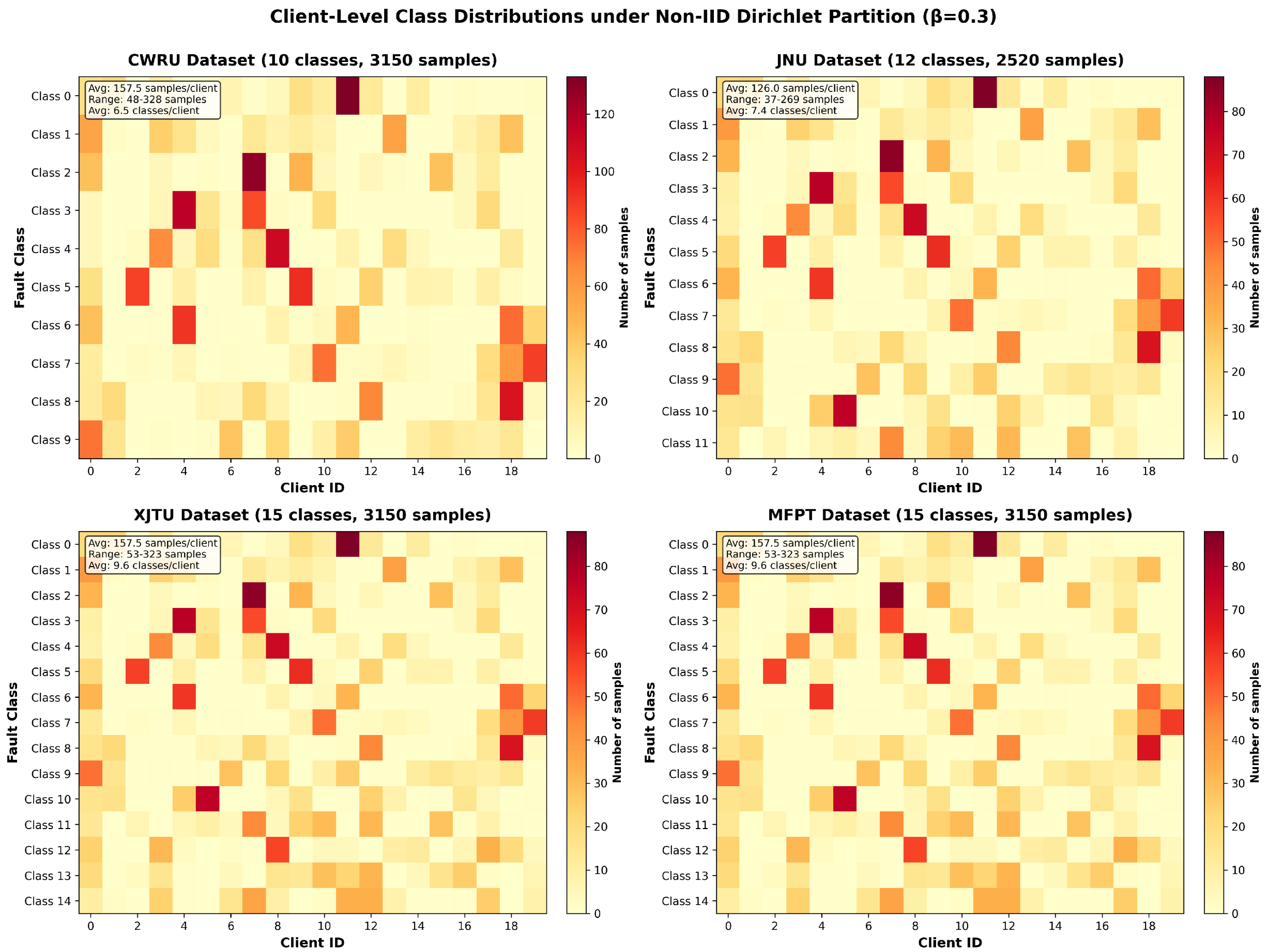
Table A2.
Client-level sample and class statistics under non-IID partitioning with Dirichlet and minimum-sample threshold . The minimum sample counts correspond to the smallest number of training windows assigned to any client after applying Algorithm A1.
Appendix A.2. Convergence Behavior Analysis
Although the previous sections report final diagnostic accuracy and communication–accuracy trade-offs, convergence behavior is also important for practical IIoT deployment. In particular, FedAnchor introduces server-side online policy learning for adaptive submodel allocation, which may raise concerns about early-stage convergence delay compared with static allocation methods. To examine this issue, we provide a representative convergence comparison of CWRU under the heterogeneous memory configuration and the Dirichlet label-skew non-IID partition with .
Figure A2.
Representative convergence behavior on CWRU under heterogeneous memory configuration and Dirichlet label–skew non-IID partition with . Curves are averaged over three fixed seeds , and shaded regions denote empirical standard deviation. (a) Test accuracy versus communication rounds. (b) Training loss versus communication rounds. (c) Early-stage test accuracy during the first 20 communication rounds.
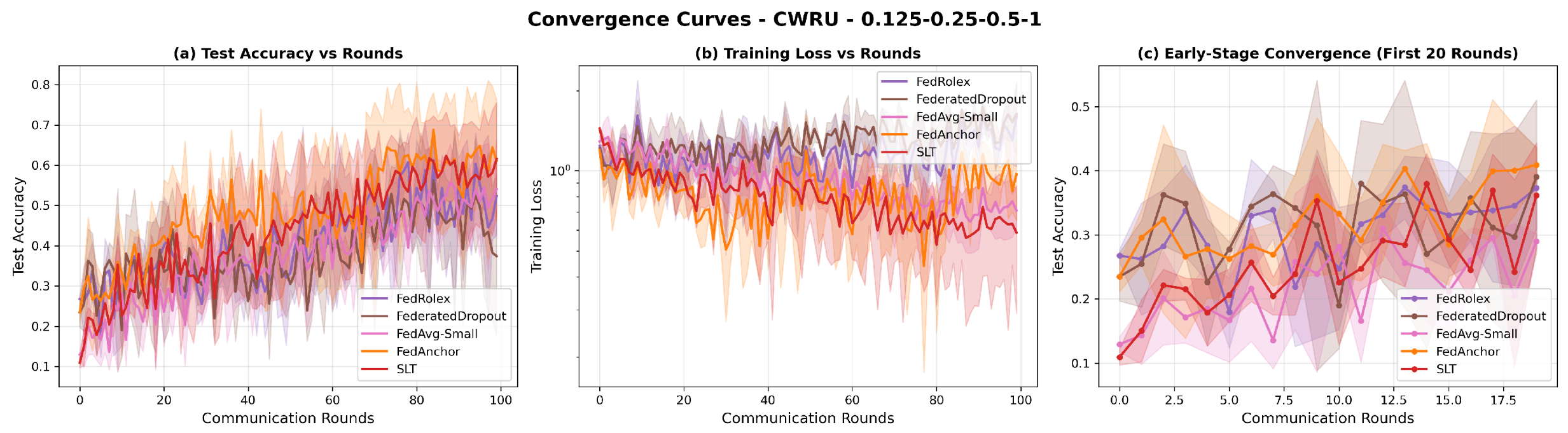
Figure A2a shows that FedAnchor does not suffer from an obvious early-stage convergence delay despite the use of server-side online policy learning. In the first 20 communication rounds, as enlarged in Figure A2c, FedAnchor improves test accuracy at a rate comparable to or faster than the representative baselines. This indicates that the fixed anchored subset provides a stable aggregation path from the beginning of training, while the DRL policy gradually adapts the non-anchored extension within the feasible memory budget.
Figure A2b further shows that FedAnchor converges smoothly without divergence or severe oscillation. Although FedAvg-Small may exhibit lower training loss in later rounds, this does not necessarily translate into better test accuracy under non-IID and resource-constrained settings. FedAvg-Small uses the smallest homogeneous feasible model to satisfy all client budgets, whereas FedAnchor allows higher-resource clients to exploit additional adaptive capacity while preserving a shared anchored aggregation subspace. Therefore, the convergence curves support the interpretation that FedAnchor balances adaptive allocation and aggregation stability rather than relying on server-side policy learning alone.
Regarding practical deployment time, FedAnchor should not be interpreted as minimizing raw wall-clock training time. As reported in Table 12, FedAnchor requires 19.5 s per round and 32.5 min for 100 rounds in the single-machine sequential simulation compared with 15.0 s per round and 25.0 min for FedAvg-Small. The additional overhead comes from adaptive submodel management and server-side policy optimization. Therefore, the practical advantage of FedAnchor lies in achieving a favorable communication–accuracy trade-off with manageable server-side overhead rather than being the fastest method in raw training time. In communication-limited IIoT deployments, reducing transmitted model traffic while improving diagnostic accuracy can be more valuable than minimizing server-side computation time alone.
Appendix A.3. Robustness Under Feature Distribution Shift
To evaluate whether FedAnchor remains effective beyond Dirichlet label-skew non-IID, we further test representative baselines under the feature-shift partition defined in Algorithm A2. This setting simulates industrial scenarios where different clients operate under different working conditions or acquisition periods, leading to shifts in vibration-signal feature distributions even when the same fault categories are observed. Unlike Dirichlet label skew, where clients have different class distributions, the feature-shift setting ensures that each client has access to all fault classes but receives different feature blocks within each class.
Unless otherwise specified, we use the representative four-tier memory configuration , clients, five selected clients per round, and three fixed random seeds . Table A3 reports the diagnostic accuracy under feature-shift non-IID.
Table A3.
Diagnostic accuracy under the feature distribution shift non-IID setting. Results are reported under the representative four-tier memory configuration . All values are mean accuracy ± standard deviation over three fixed seeds . Bold values indicate the highest accuracy for each dataset.
The results show that feature-shift non-IID presents a different optimization challenge from Dirichlet label skew. Under feature shift, clients have access to all fault classes, but the feature statistics within each class differ across clients. This setting therefore tests whether the learned global representation remains stable when the heterogeneity comes from signal characteristics rather than class imbalance.
FedAnchor achieves the highest accuracy across all four datasets under this additional non-IID mode. Compared with FedAvg-Small, FedAnchor improves accuracy by 10.42, 14.31, 9.39, and 10.17 percentage points on CWRU, JNU, MFPT, and XJTU, respectively. The improvement indicates that the anchored shared subspace remains useful when clients have balanced class coverage but shifted feature distributions. The adaptive extension further allows clients with different memory budgets to exploit feasible model capacity without forcing all clients to train the weakest homogeneous model.
These results complement the Dirichlet label-skew experiments and show that FedAnchor is not only effective under a single non-IID partition type. They also suggest that industrial federated fault diagnosis should evaluate both label-distribution skew and feature-distribution shifts, because these two forms of heterogeneity impose different challenges on local training and global aggregation.
Appendix A.4. Robustness to Client Selection Policies
The main experiments use uniform random client selection with five clients per round. Although this protocol is widely used for partial-participation FL and provides a method-independent evaluation setting, it may introduce round-wise variation in the memory-tier composition of selected clients under resource heterogeneity. Such variation could potentially affect the update frequency of different submodel components and the stability of anchored-parameter aggregation.
To examine this effect, we conduct an additional sensitivity study on client selection policies. We compare the default random selection with two alternatives: tier-balanced selection and round-robin selection. Random selection samples clients uniformly without replacement from all clients. Tier-balanced selection explicitly controls the memory-tier composition of each selected client set; under the representative four-tier configuration , one client is sampled from each tier, and the fifth client is assigned to a tier in a rotating manner across rounds. Round-robin selection follows a deterministic cyclic schedule to ensure that all clients participate approximately the same number of times during training.
All policies use the same number of selected clients per round, the same total number of communication rounds, and the same local training settings. The experiments are conducted under the representative four-tier memory configuration and Dirichlet label-skew non-IID partition with . All values are reported over the three fixed seeds .
Table A4.
Effect of client selection policies on FedAnchor under the representative four-tier memory configuration and Dirichlet label-skew non-IID partition with . All values are mean accuracy ± standard deviation over the three fixed seeds .
Table A4 shows that FedAnchor remains stable across different client selection policies. Compared with random selection, tier-balanced selection slightly reduces the round-wise fluctuation of selected resource tiers, leading to a marginal average improvement of 0.22 percentage points across datasets. Round-robin selection ensures more uniform long-term participation across clients and achieves performance comparable to random selection, with an average difference of only percentage points. Overall, the diagnostic accuracy varies by less than 0.3 percentage points across the three policies, indicating that FedAnchor is not overly dependent on a particular random client selection sequence.
This robustness can be attributed to the anchored submodel design. The anchored subset is retained by every selected client regardless of its memory tier. Therefore, even when the adaptive extension varies with client resources, the anchored parameters still receive updates from the selected participants in every communication round. This design helps maintain a shared diagnostic representation under partial participation, while the adaptive extension accommodates resource-specific capacity differences. In addition, the random sequence used in the main experiments is fixed per seed and shared across all compared methods, which prevents client-selection randomness from favoring a particular algorithm.
The small improvement observed under tier-balanced selection suggests that explicitly controlling the memory-tier composition can provide additional stability by reducing round-wise fluctuation in the distribution of selected resource tiers. However, FedAnchor under random selection already achieves competitive performance, indicating that the anchoring mechanism mitigates much of the update inconsistency caused by resource-heterogeneous participation without requiring controlled selection policies.
Appendix A.5. Activation and Signal-Level Analysis of Anchored Parameters
To further examine the signal-level behavior of anchored channels in industrial fault diagnosis, we analyze the learned first-layer filters and their activation responses. This analysis is intended to clarify whether the anchored subspace preserves common fault-discriminative information rather than to claim a manually predefined correspondence between anchored neurons and specific physical frequency bands.
Filter Frequency Response: For the first convolutional layer, we compute the normalized frequency response of each learned kernel. For a convolutional kernel , the normalized response is defined as
where denotes the Fourier transform, and is a small constant for numerical stability. We average over anchored and non-anchored channels, respectively, to compare the spectral regions emphasized by the two channel groups.
Activation Energy: For an input sample x, let denote the activation map of channel j in layer ℓ. For a channel subset , where can be the anchored subset or the non-anchored subset, the activation energy is computed as
where denotes the temporal length of the activation map.
Figure A3.
Signal-level interpretation of anchored and non-anchored channels. The visualization is obtained from the first convolutional layer of FedAnchor on CWRU under heterogeneous memory configurations and the non-IID partition with Dirichlet . (a,b) Average frequency responses of first-layer convolutional filters in the anchored and non-anchored subsets, with a unified y-axis for fair comparison. Anchored filters are not manually tied to predefined frequency bands; instead, they exhibit more concentrated and stable responses in fault-sensitive spectral regions through repeated cross-client updates. (c,d) Activation energy heatmaps on test samples ordered by class, with a unified colorbar and colormap for fair comparison. Dashed vertical lines indicate a selected fault-class segment. Anchored channels show more consistent fault-related activation patterns across the fault segment, whereas non-anchored channels retain more dispersed and client-specific adaptive responses.
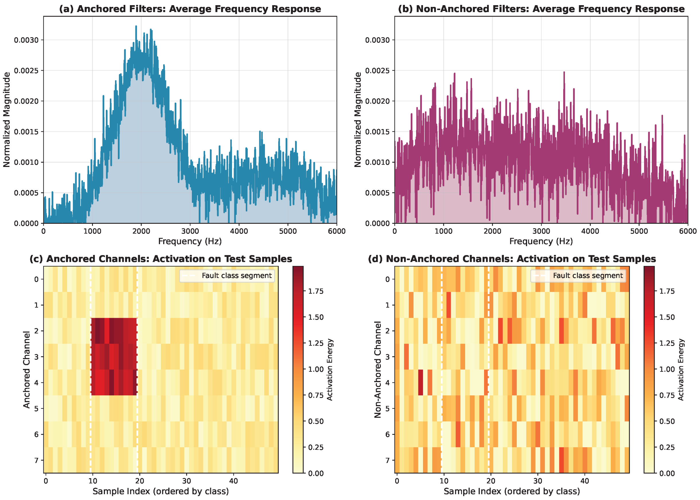
Figure A3 provides a signal-level comparison between anchored and non-anchored channels. The frequency–response curves show that anchored filters do not correspond to a single manually specified frequency band. Instead, they form a group of learnable filters with more concentrated spectral responses after federated training. Compared with the anchored filters, the non-anchored filters exhibit more dispersed responses over the frequency range, which is consistent with their role as client-specific adaptive extensions.
The activation heatmaps further show that anchored channels produce more concentrated responses on the representative fault-class segment. In contrast, the non-anchored channels exhibit more scattered activation patterns. This observation suggests that the anchored subset tends to preserve common fault-discriminative information that is repeatedly updated across clients, whereas the non-anchored subset mainly provides additional adaptive capacity for client-specific variations. Therefore, the signal-level analysis supports the motivation of FedAnchor: anchoring does not impose predefined physical features but encourages a shared set of learnable diagnostic filters that helps stabilize aggregation under structural heterogeneity.
As a qualitative diagnostic visualization, this analysis should not be interpreted as a deterministic mapping between anchored channels and physical bearing-characteristic frequencies. Instead, it provides empirical evidence that the repeatedly updated anchored subset develops more stable fault-related spectral and activation responses under the evaluated federated setting.
References
- Zhu, Z.; Lei, Y.; Qi, G.; Chai, Y.; Mazur, N.; An, Y.; Huang, X. A review of the application of deep learning in intelligent fault diagnosis of rotating machinery. Measurement 2023, 206, 112346. [Google Scholar] [CrossRef] [Scilit]
- Hoang, D.T.; Kang, H.J. A survey on deep learning based bearing fault diagnosis. Neurocomputing 2019, 335, 327–335. [Google Scholar] [CrossRef] [Scilit]
- Zhang, F.; Li, Z.; Cheng, Y.; Yang, Y.; Han, Y.; Yi, C.; Li, T.; Yan, J.; Dong, L.; Zhang, W. MHSNet: A Multi-Scale Hidden State Interaction Network for Fault Diagnosis of Rotating Machinery. Tsinghua Sci. Technol. 2025, 31, 2855–2876. [Google Scholar] [CrossRef] [Scilit]
- Zou, L.; Ling, H.; Lei, M.; Fang, X.; Cai, M.; Yu, H. Domain-Independent Gear Pitting Fault Diagnosis Using Transformer Encoder and LinSoftmax. Big Data Min. Anal. 2025, 8, 1127–1147. [Google Scholar] [CrossRef] [Scilit]
- The European Parliament and the Council of the European Union. Regulation (EU) 2016/679 of the European Parliament and of the Council; Official Journal of the European Union: Brussels, Belgium, 2016. [Google Scholar]
- Qian, Q.; Zhang, B.; Li, C.; Mao, Y.; Qin, Y. Federated transfer learning for machinery fault diagnosis: A comprehensive review of technique and application. Mech. Syst. Signal Process. 2025, 223, 111837. [Google Scholar] [CrossRef] [Scilit]
- Zhang, W.; Li, X.; Ma, H.; Luo, Z.; Li, X. Federated learning for machinery fault diagnosis with dynamic validation and self-supervision. Knowl.-Based Syst. 2021, 213, 106679. [Google Scholar] [CrossRef] [Scilit]
- Jiang, H.; Chen, S.; Ouyang, T.; Lin, M.; Zhang, X.; Zhang, Q.; Chen, X. MFEL-H2B: Multimodal Federated Edge Learning with heterogeneity-aware balancing across modalities and models. High-Confid. Comput. 2026, 100384. [Google Scholar] [CrossRef] [Scilit]
- Yang, T.; Andrew, G.; Eichner, H.; Sun, H.; Li, W.; Kong, N.; Ramage, D.; Beaufays, F. Applied federated learning: Improving google keyboard query suggestions. arXiv 2018, arXiv:1812.02903. [Google Scholar]
- Maeng, K.; Lu, H.; Melis, L.; Nguyen, J.; Rabbat, M.; Wu, C.J. Towards fair federated recommendation learning: Characterizing the inter-dependence of system and data heterogeneity. In Proceedings of the 16th ACM Conference on Recommender Systems, Seattle, WA, USA, 18–23 September 2022; pp. 156–167. [Google Scholar]
- Wu, M.; Li, L.; Chang, T.; Qiao, P.; Miao, C.; Zhou, J.; Wang, J.; Wang, X. FedEKT: Ensemble Knowledge Transfer for Model-Heterogeneous Federated Learning. In Proceedings of the 2024 IEEE/ACM 32nd International Symposium on Quality of Service (IWQoS), Guangzhou, China, 19–21 June 2024; pp. 1–10. [Google Scholar]
- Qiao, Y.; Adhikary, A.; Kim, K.T.; Zhang, C.; Hong, C.S. Knowledge distillation assisted robust federated learning: Towards edge intelligence. In Proceedings of the ICC 2024-IEEE International Conference on Communications, Denver, CO, USA, 9–13 June 2024; pp. 843–848. [Google Scholar]
- He, C.; Annavaram, M.; Avestimehr, S. Group knowledge transfer: Federated learning of large cnns at the edge. Adv. Neural Inf. Process. Syst. 2020, 33, 14068–14080. [Google Scholar]
- Caldas, S.; Konečny, J.; McMahan, H.B.; Talwalkar, A. Expanding the reach of federated learning by reducing client resource requirements. arXiv 2018, arXiv:1812.07210. [Google Scholar]
- Wang, I.; Nair, P.; Mahajan, D. Fluid: Mitigating stragglers in federated learning using invariant dropout. Adv. Neural Inf. Process. Syst. 2024, 36, 73258–73273. [Google Scholar]
- Alam, S.; Liu, L.; Yan, M.; Zhang, M. Fedrolex: Model-heterogeneous federated learning with rolling sub-model extraction. Adv. Neural Inf. Process. Syst. 2022, 35, 29677–29690. [Google Scholar] [CrossRef] [Scilit]
- Ma, H.; Wei, J.; Zhang, G.; Wang, Q.; Kong, X.; Du, J. Heterogeneous Federated Learning: Client-side Collaborative Update Inter-Domain Generalization Method for Intelligent Fault Diagnosis. IEEE Internet Things J. 2024, 12, 5704–5718. [Google Scholar]
- Kulevome, D.K.B.; Man, Q.; Mawuli, E.S.; Opoku-Mensah, E. Personalized Federated Learning with Kolmogorov-Arnold Enhanced CNN for Rotating Equipment Fault Diagnosis. In Proceedings of the 2024 21st International Computer Conference on Wavelet Active Media Technology and Information Processing (ICCWAMTIP), Chengdu, China, 14–16 December 2024; pp. 1–5. [Google Scholar]
- Cui, J.; Li, J.; Mei, Z.; Wei, K.; Wei, S.; Ding, M.; Chen, W.; Guo, S. Federated meta-learning for few-shot fault diagnosis with representation encoding. IEEE Trans. Instrum. Meas. 2023, 72, 3536812. [Google Scholar] [CrossRef] [Scilit]
- Li, X.; Zhang, C.; Li, X.; Zhang, W. Federated transfer learning in fault diagnosis under data privacy with target self-adaptation. J. Manuf. Syst. 2023, 68, 523–535. [Google Scholar] [CrossRef] [Scilit]
- Yan, Z.; Xu, Z.; Zhang, Y.; Sun, J.; Liu, L.; Sun, Y. FTSDC: A novel federated transfer learning strategy for bearing cross-machine fault diagnosis based on dual-correction training. Adv. Eng. Inform. 2024, 61, 102499. [Google Scholar] [CrossRef] [Scilit]
- Guo, S.; Chen, H.; Liu, Y.; Yang, C.; Li, Z.; Jin, C.H. Heterogeneous Federated Learning Framework for IIoT Based on Selective Knowledge Distillation. IEEE Trans. Ind. Inform. 2024, 21, 1078–1089. [Google Scholar] [CrossRef] [Scilit]
- Horvath, S.; Laskaridis, S.; Almeida, M.; Leontiadis, I.; Venieris, S.; Lane, N. Fjord: Fair and accurate federated learning under heterogeneous targets with ordered dropout. Adv. Neural Inf. Process. Syst. 2021, 34, 12876–12889. [Google Scholar]
- Diao, E.; Ding, J.; Tarokh, V. Heterofl: Computation and communication efficient federated learning for heterogeneous clients. arXiv 2020, arXiv:2010.01264. [Google Scholar]
- Nader, B.; Jiahui, H.; Hui, Z.; Xin, L. Adaptive federated dropout: Improving communication efficiency and generalization for federated learning. In Proceedings of the Proceedings of the IEEE Conference on Computer Communications Workshops, Vancouver, BC, Canada, 10–13 May 2021; pp. 10–13. [Google Scholar]
- Pfeiffer, K.; Khalili, R.; Henkel, J. Aggregating capacity in FL through successive layer training for computationally-constrained devices. Adv. Neural Inf. Process. Syst. 2023, 36, 35386–35402. [Google Scholar] [CrossRef] [Scilit]
- Shamsian, A.; Navon, A.; Fetaya, E.; Chechik, G. Personalized Federated Learning using Hypernetworks. In Proceedings of the 38th International Conference on Machine Learning; Meila, M., Zhang, T., Eds.; PMLR: New York, NY, USA, 2021; Volume 139, pp. 9489–9502. [Google Scholar]
- Litany, O.; Maron, H.; Acuna, D.; Kautz, J.; Chechik, G.; Fidler, S. Federated learning with heterogeneous architectures using graph hypernetworks. arXiv 2022, arXiv:2201.08459. [Google Scholar]
- Wang, R.; Yu, T.; Zhang, R.; Kim, S.; Rossi, R.; Zhao, H.; Wu, J.; Mitra, S.; Yao, L.; Henao, R. Personalized federated learning for text classification with gradient-free prompt tuning. In Proceedings of the Findings of the Association for Computational Linguistics: NAACL 2024, Mexico City, Mexico, 16–21 June 2024; Association for Computational Linguistics: Stroudsburg, PA, USA, 2024; pp. 4597–4612. [Google Scholar]
- Kang, H.; Cha, S.; Shin, J.; Lee, J.; Kang, J. Nefl: Nested model scaling for federated learning with system heterogeneous clients. IEEE Trans. Mob. Comput. 2025, 24, 6734–6746. [Google Scholar] [CrossRef] [Scilit]
- Wu, F.; Wang, X.; Wang, Y.; Liu, T.; Su, L.; Gao, J. Fiarse: Model-heterogeneous federated learning via importance-aware submodel extraction. Adv. Neural Inf. Process. Syst. 2024, 37, 115615–115651. [Google Scholar] [CrossRef] [Scilit]
- Lillicrap, T. Continuous control with deep reinforcement learning. arXiv 2015, arXiv:1509.02971. [Google Scholar]
- McMahan, B.; Moore, E.; Ramage, D.; Hampson, S.; y Arcas, B.A. Communication-efficient learning of deep networks from decentralized data. In Proceedings of the Artificial Intelligence and Statistics, Lauderdale, FL, USA, 20–22 April 2017; PMLR: New York, NY, USA, 2017; pp. 1273–1282. [Google Scholar]
- Paszke, A.; Gross, S.; Massa, F.; Lerer, A.; Bradbury, J.; Chanan, G.; Killeen, T.; Lin, Z.; Gimelshein, N.; Antiga, L.; et al. Pytorch: An imperative style, high-performance deep learning library. Adv. Neural Inf. Process. Syst. 2019, 32, 8026–8037. [Google Scholar]
- Smith, W.A.; Randall, R.B. Rolling element bearing diagnostics using the Case Western Reserve University data: A benchmark study. Mech. Syst. Signal Process. 2015, 64, 100–131. [Google Scholar] [CrossRef] [Scilit]
- Li, K.; Ping, X.; Wang, H.; Chen, P.; Cao, Y. Sequential fuzzy diagnosis method for motor roller bearing in variable operating conditions based on vibration analysis. Sensors 2013, 13, 8013–8041. [Google Scholar] [CrossRef] [Scilit] [PubMed]
- Wang, B.; Lei, Y.; Li, N.; Li, N. A Hybrid Prognostics Approach for Estimating Remaining Useful Life of Rolling Element Bearings. IEEE Trans. Reliab. 2020, 69, 401–412. [Google Scholar] [CrossRef] [Scilit]
- MFPT. Fault Data Sets. 2013. Available online: http://www.mfpt.org/ (accessed on 10 April 2013).
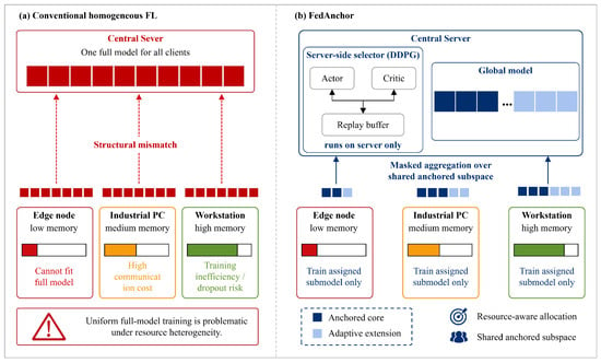
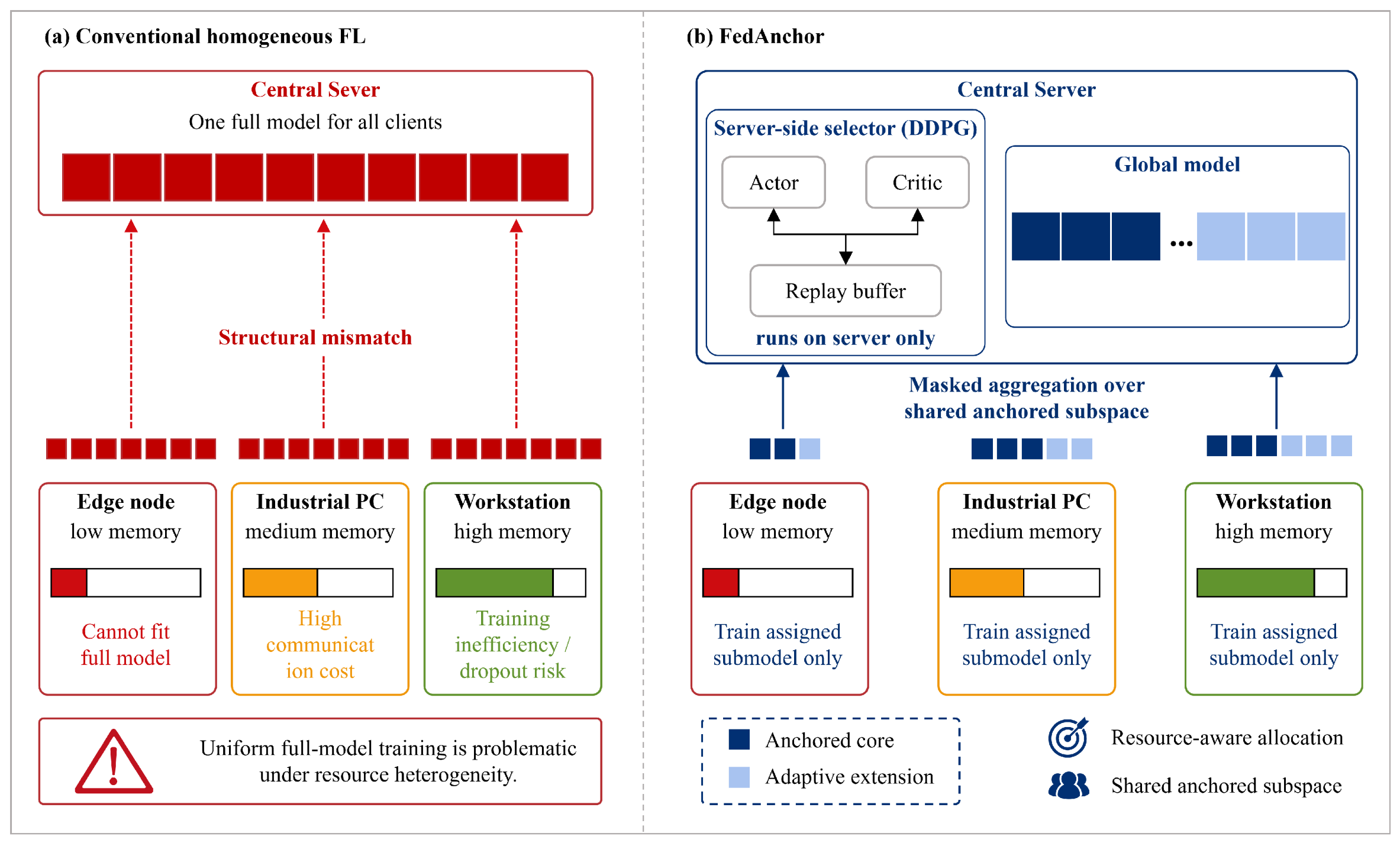
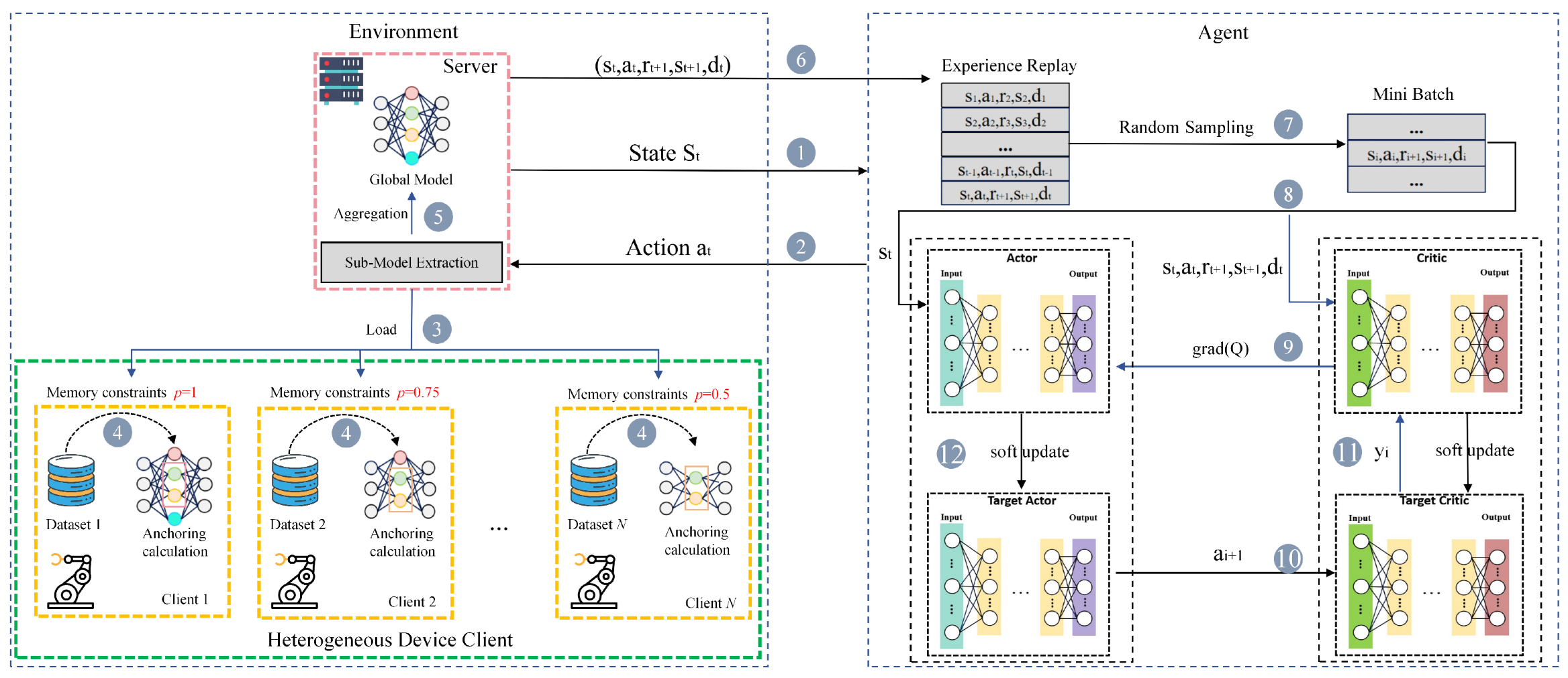
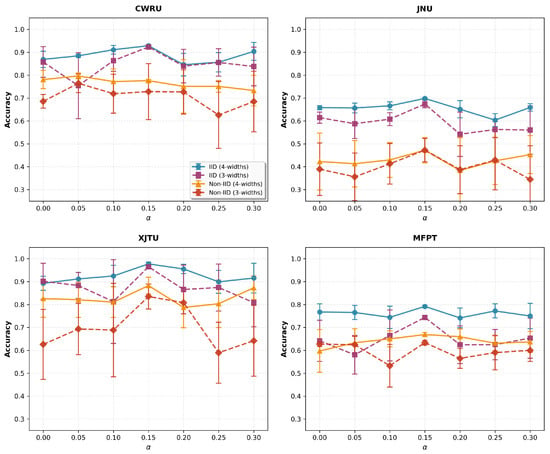
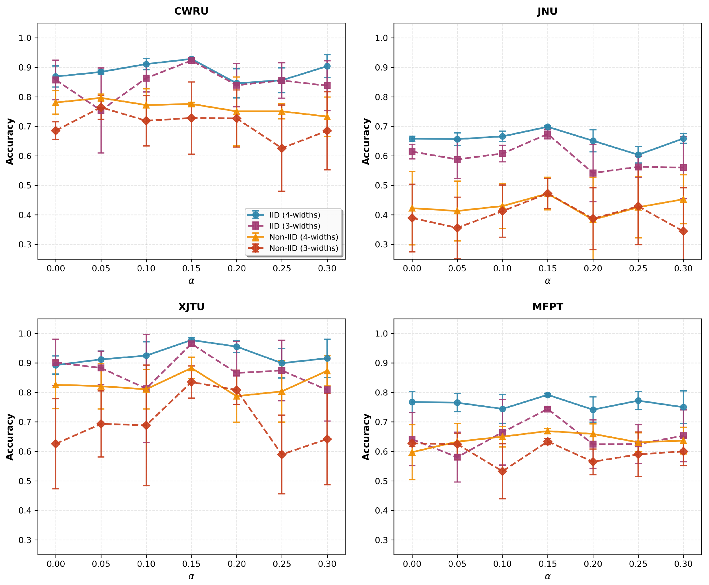
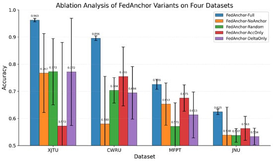
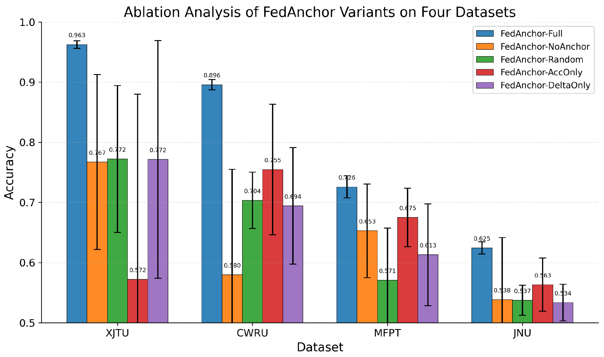

Disclaimer/Publisher’s Note: The statements, opinions and data contained in all publications are solely those of the individual author(s) and contributor(s) and not of MDPI and/or the editor(s). MDPI and/or the editor(s) disclaim responsibility for any injury to people or property resulting from any ideas, methods, instructions or products referred to in the content. |
© 2026 by the authors. Licensee MDPI, Basel, Switzerland. This article is an open access article distributed under the terms and conditions of the Creative Commons Attribution (CC BY) license.