


Abstract
Stewart parallel mechanisms are widely used in motion simulation, posture adjustment, and active compensation owing to their high stiffness, high load capacity, and high positioning accuracy. However, under unknown paths or time-varying target trajectories, their strong multi-chain coupling, limited workspace, and configuration-dependent motion capability may cause actuator velocity and acceleration violations, especially near workspace boundaries or low-mobility regions. Moreover, conventional online trajectory scaling methods are usually designed for acceleration bounds with regular positive and negative limits. After nonlinear kinematic constraint mapping, the acceleration bounds of a Stewart mechanism in the path-parameter space may become same-signed, shifted, or abruptly varying, which can lead to planning failure or motion discontinuity. To address these problems, this paper proposes a condition-number-aware velocity bound regulation scaling method for online trajectory planning under unknown paths. Path–velocity decomposition is first used to transform the six-degree-of-freedom trajectory planning problem into a path-time-law planning problem, and actuator constraints are mapped into the path-parameter space. Then, a workspace classification model and the dimensionless Jacobian condition number are introduced to evaluate local motion capability. Based on the workspace level and condition number, a hierarchical scaling factor is designed to adaptively adjust the path velocity boundary. In addition, the conventional trajectory scaling method is improved by introducing a special acceleration-bound handling mechanism. Single-axis and platform experimental results show that the proposed method can effectively handle special acceleration bounds, reduce actuator constraint violations, and improve the safety and continuity of online trajectory planning.
1. Introduction
Parallel mechanisms have been widely used in precision manufacturing, motion simulation, active stabilization, and complex equipment testing because of their high stiffness, high load capacity, compact structure, and high positioning accuracy [1,2,3]. As a representative six-degree-of-freedom parallel mechanism, the Stewart platform can realize coupled translational and rotational motions and has been applied in motion simulators, wave compensation systems, spacecraft docking, and dynamic posture adjustment devices [4,5].
However, trajectory planning for Stewart mechanisms is challenging due to multi-chain coupling, limited workspace, and configuration-dependent constraints. The desired end-effector motion must be mapped into the length, velocity, acceleration, and driving force of six actuated limbs. When the platform configuration changes, the Jacobian matrix, workspace boundary, singularity state, and local motion capability also vary [6]. Therefore, a trajectory that is feasible in one configuration may cause actuator saturation, acceleration violation, or reduced controllability in another configuration. This problem becomes more evident in online tasks with unknown paths, target changes, or limited future information.
Path–velocity decomposition (PVD) provides an effective framework for constrained trajectory planning. It separates a trajectory into a geometric path and a path time law, thereby converting a multi-dimensional trajectory planning problem into a one-dimensional velocity planning problem along the path parameter [7,8,9]. Based on this idea, time-optimal path parameterization and reachability-analysis-based methods have been developed to generate feasible path time laws under velocity, acceleration, and dynamic constraints [10,11,12]. For Stewart mechanisms, PVD enables the actuator constraints of the six limbs to be mapped into the path-parameter space, which provides a basis for boundary construction and online trajectory scaling.
Online trajectory scaling methods based on nonlinear filters or variable-structure filters can modify the path time law in real time according to velocity and acceleration bounds [13,14]. These methods are computationally efficient and suitable for real-time implementation. Further studies have considered asymmetric, time-varying, or higher-order constraints to improve the robustness of online trajectory generation [15,16,17,18]. Nevertheless, most existing methods assume that the acceleration bounds have a regular lower–upper structure. For Stewart mechanisms, nonlinear constraint mapping may lead to special acceleration bounds in the path-parameter space, such as same-signed bounds, shifted feasible intervals, or abrupt boundary variations. Under these conditions, conventional trajectory scaling may suffer from overshoot, discontinuity, or planning failure.
Another limitation is that many trajectory planning methods require a known or predictable path. In unknown-path tasks, the complete geometric path is unavailable, and the planner can only construct local paths from the current state to the next target. If the planner only considers instantaneous actuator constraints, the mechanism may gradually approach workspace boundaries or low-mobility regions. Although workspace analysis and singularity evaluation have been widely used in mechanism design and offline path planning [19,20], they are rarely integrated into online trajectory scaling. For Stewart mechanisms, online planning should not only satisfy limb constraints but also adjust motion capability according to the current workspace region and local kinematic performance.
To address these issues, this paper proposes a condition-number-aware velocity bound regulation scaling method for online trajectory planning of Stewart mechanisms under unknown paths. In each control cycle, a local path is generated from the current pose and the local target, and the actuator velocity and acceleration constraints are mapped into the path-parameter space. A workspace classification model and a dimensionless Jacobian condition number are then used to evaluate the current motion capability. Based on this evaluation, hierarchical scaling factors are applied to regulate the velocity and acceleration bounds. In addition, the conventional trajectory scaling method is improved by introducing a special acceleration-bound handling mechanism, allowing feasible path acceleration commands to be generated under same-signed, shifted, or abruptly varying acceleration bounds.
The main contributions of this paper are as follows.
- A PVD-based online trajectory planning framework is established for Stewart mechanisms under unknown paths, in which actuator velocity and acceleration constraints are mapped into the path-parameter space.
- A condition-number-aware velocity bound regulation method is proposed. Workspace classification and the dimensionless Jacobian condition number are combined to evaluate local motion capability, and the path velocity boundary is adjusted according to the current workspace level and kinematic performance.
- The conventional trajectory scaling method is improved to handle special acceleration bounds caused by nonlinear constraint mapping, including same-signed, shifted, and abruptly varying bounds.
2. Materials and Methods
2.1. Online Trajectory Planning Framework Under Unknown Paths
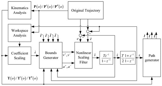
The online trajectory planning framework under unknown paths is shown in Figure 1. The framework is constructed based on path–velocity decomposition and nonlinear trajectory scaling. First, the original trajectory is decomposed into geometric path information and path time-law information through path interpolation and kinematic analysis. In this process, the direct mapping relationship between the end-effector trajectory and the motions of the six actuated limbs is established and denoted as . The mapping , together with its first- and second-order derivatives, is used to describe the relationship between the path parameter and the actuator displacement, velocity, and acceleration.
Figure 1.
Online trajectory planning framework under unknown paths.
Meanwhile, the path information and the current motion state are introduced into the workspace analysis module. By evaluating the current workspace region and local motion capability, the coefficient scaling module calculates the boundary scaling coefficient . This coefficient is used to adjust the original motion constraints before they are sent to the bounds generator. Then, the bounds generator constructs the velocity and acceleration limits suitable for the nonlinear scaling filter. These limits are expressed in the path-parameter space and reflect both the actuator constraints and the workspace-related safety margin.
After the feasible bounds are obtained, the nonlinear scaling filter modifies the path time law according to the tracking error, the current path state, and the scaled constraints. Instead of changing the geometric path, the filter adjusts the path velocity and path acceleration in real time. The scaled path time law is then sent to the path generator, which reconstructs the feasible trajectory and outputs the final control command. Through this closed-loop structure, the proposed framework can continuously update the trajectory according to the current state, actuator constraints, and workspace conditions.
2.2. Trajectory–Actuator Mapping Based on Inverse Kinematics
In the proposed online trajectory planning framework, the original trajectory is first decomposed into geometric path information and path time-law information. The geometric path determines the pose variation in the moving platform, while the time law determines the motion rate along the path. To generate actuator-level constraints for the nonlinear scaling filter, the relationship between the path parameter and the actuator motion should be established through kinematic analysis. This relationship is defined as the trajectory–actuator mapping.
To construct the actuator constraints used by the nonlinear scaling filter, the end-effector trajectory should first be mapped to the actuator space. Let the geometric path of the moving platform be expressed as
where is the path parameter, and is the pose vector of the moving platform.
For the -th limb, the inverse kinematic equation is
where is the fixed-platform joint position, is the moving-platform joint position expressed in the moving coordinate system, is the position vector of the moving platform center, and is the rotation matrix of the moving platform.
For the Stewart mechanism, the inverse kinematic relationship can be written as
where is the actuator length vector, and denotes the inverse kinematic function. By substituting the geometric path into the inverse kinematic model, the trajectory–actuator mapping is obtained as
Thus, the actuator displacement corresponding to the path parameter is
Differentiating the inverse kinematic relationship with respect to time, the velocity-level inverse kinematics of the Stewart mechanism can be written as
where is the velocity Jacobian matrix of the mechanism. This equation describes the mapping from the moving-platform velocity to the actuator velocities.
Since the geometric path is expressed as (1), the end-effector velocity is obtained as
Substituting this expression into the velocity inverse kinematics gives
Since the trajectory–actuator mapping is defined as (6), its time derivative can also be written as
where .
This relationship is used to map actuator velocity constraints into the path-parameter space.
Differentiating the velocity-level inverse kinematics, the acceleration-level inverse kinematics can be expressed as
where is the velocity-dependent nonlinear term caused by configuration variation.
For the acceleration-level inverse kinematics, the second-order trajectory–actuator mapping is defined as
where is the derivative of the Jacobian matrix with respect to the path parameter. Therefore, the actuator acceleration can be directly expressed as
Substituting and into the above equation gives the complete acceleration-level inverse kinematic relationship:
This equation indicates that the actuator acceleration is affected by both the path acceleration and the path velocity . The term related to reflects the nonlinear influence of path curvature and configuration variation.
2.3. Bound Generation and Improved Trajectory Scaling
Based on the trajectory–actuator mapping obtained in Section 2.2, the bounds generator converts the actuator velocity and acceleration limits into the feasible bounds of the path time law. For the -th actuator, the velocity bound of the path parameter is first calculated as
where and are the lower and upper velocity limits of the -th actuator, respectively.
For a monotonic path parameter, the lower bound is usually set to zero, and the velocity constraint becomes
with
Similarly, the acceleration bound of the path parameter is generated from the actuator acceleration constraints. For the -th actuator, the acceleration constraint is
According to the acceleration mapping in Section 2.2, the actuator acceleration is affected by both and . Therefore, the acceleration bound contributed by the -th actuator can be expressed as
By intersecting the acceleration constraints of all six actuators, the global acceleration bounds are obtained as
Thus, the acceleration constraint sent to the nonlinear scaling filter is
In the general case, the acceleration bounds generated by the bounds generator satisfy which means that both positive and negative path accelerations are feasible. However, due to the nonlinear mapping between the Stewart mechanism and the path parameter, the generated bounds may become same-signed in some configurations, namely or . In addition, when the feasible acceleration interval does not exist, indicating that no path acceleration can satisfy all actuator constraints at the current state. Since the conventional trajectory scaling method is mainly designed for the regular case , it is necessary to improve the scaling process to handle same-signed or infeasible acceleration bounds.
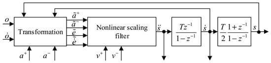
When the bounds generated by the bounds generator satisfy this condition, the original input variables are directly used. When the acceleration bounds do not satisfy this condition, the proposed method introduces a converter before the nonlinear scaling filter. The converter reconstructs the local input variables in the current sampling period so that the transformed acceleration bounds satisfy the regular form required by the conventional filter, as shown in Figure 2.
Figure 2.
Structure of the improved trajectory scaling filter with trajectory transformation.
When the acceleration bounds have the same sign, an acceleration offset is introduced to transform the original acceleration interval into an equivalent interval containing zero.
where is a small positive value. To make the converted system equivalent in the current sampling period, the reference input is modified as
The converted acceleration bounds are
Thus,
The nonlinear scaling filter calculates the acceleration command under the converted bounds. The acceleration command in the original path-parameter space is then recovered by
For the velocity constraint, the reference velocity is also processed by saturation:
where the saturation operator is defined as
At the current sampling instant , the original error state is defined as
Accordingly, the transformed error state is
Therefore, the trajectory update in the original path-parameter space is performed as
where , rearranged to
This transformation does not require the next-step errors of the original and transformed systems to be identical. Instead, it ensures that the acceleration command obtained from the transformed error input can be mapped back to the original path-parameter space and produce the corresponding trajectory update result. Therefore, can be used as the input of the nonlinear scaling filter under the converted acceleration bounds.
Since the online trajectory planner updates the path state, constraint bounds, and scaling command at every sampling period, this transformation is only a local equivalent treatment within the current cycle. It does not establish a fixed long-term error model, and the approximation introduced by the transformation will not accumulate over multiple cycles.
After this transformation, the trajectory scaling process follows the nonlinear scaling method reported in Ref. [18], where the normalized error state is used to determine the acceleration command under the converted bounds.
The normalized error vector is defined as
where
The trajectory scaling problem is then converted into driving the normalized error state toward the origin. The transformed error system can be written as
After the above reconstruction, the controller can be simplified because the converted acceleration bounds satisfy the regular form required by the scaling filter. The control law is defined as follows
where is an intermediate variable used to describe the relationship between the current system state and the constraint boundaries. The calculation process is given below.
To determine the switching variable, two boundary states are first defined according to the relationship between the velocity bounds and the target velocity.
To describe the position of the system state in different regions, the piecewise variable is defined as
The control direction variable is defined as
Then, the integer parameter is calculated by
The switching variable is obtained as
According to the above definitions, the nonlinear switching surface in the plane can be expressed as
The corresponding sliding boundary is given by
Based on the switching variable , the nonlinear scaling controller determines the converted acceleration command. The command is then transformed back to the original path-parameter space and constrained by the original acceleration bounds.
Finally, the output path acceleration is constrained by the original physical bounds:
The updated path parameter is then sent to the path generator to reconstruct the feasible output trajectory. In this way, the original geometric path is preserved, while the path time law is modified according to the actuator constraints and the converted acceleration bounds. Since the conversion is performed at each sampling period, the algorithm does not rely on a fixed long-term equivalent model. Instead, it uses a local equivalent transformation to make the nonlinear scaling filter applicable to special acceleration bounds and updates the trajectory state in a receding manner.
2.4. Workspace- and Condition-Number-Based Scaling of the Velocity Boundary
For the Stewart mechanism, the reachable position range alone is not sufficient to describe the actual motion capability, because different positions may correspond to different posture-adjustment ability, constraint margins, and local kinematic performance. Therefore, the workspace is divided into three nested regions: the reachable workspace, the total-orientation workspace, and the rated workspace. The reachable workspace denotes the largest position set that the moving platform reference point can reach under basic structural constraints. The total-orientation workspace further requires that, at each position, the platform can realize the prescribed posture range while satisfying the constraints. The rated workspace is the core stable region determined by engineering requirements, where the platform has sufficient posture margin and motion capability.
The three workspaces have a hierarchical relationship. The reachable workspace has the largest range but does not guarantee complete posture capability. The total-orientation workspace is located inside the reachable workspace and ensures that the required posture range is available. The rated workspace is located inside the total-orientation workspace and corresponds to the preferred operating region for online trajectory planning. Therefore, in the proposed method, the rated workspace is treated as the safe inner region, the remaining part of the total-orientation workspace is treated as the intermediate region, and the area outside the total-orientation workspace but still within the reachable workspace is treated as the outer region with degraded motion capability.
After the current workspace region is identified, the local motion capability is evaluated using the dimensionless Jacobian condition number. Since the Stewart mechanism contains both translational and rotational motion components, the original Jacobian matrix should be normalized before calculating the condition number. Let the Jacobian matrix at the current pose be divided into translational and rotational parts:
where is the translational part and is the rotational part. To balance the numerical scales of the two parts, a length-related scaling coefficient is introduced. The dimensionless Jacobian matrix is constructed as
where is calculated by
Based on the dimensionless Jacobian matrix, the condition number is defined as
where and are the maximum and minimum singular values of , respectively. A smaller indicates better local motion transmission, whereas a larger indicates that the mechanism is approaching a low-mobility or near-singular region.
To further guarantee the overall motion capability, the scaled velocity boundary is combined with the joined velocity boundary. The joined velocity boundary is introduced to ensure that the corresponding acceleration bounds remain feasible, namely and . Therefore, the final velocity boundary sent to the nonlinear scaling filter is expressed as
The joined velocity boundary can be expressed as
where denotes the maximum path velocity that guarantees the regular acceleration condition and . After the joined velocity boundary is obtained, the scaling coefficient is applied as
where is the velocity scaling coefficient. In the rated workspace, the mechanism has sufficient motion margin, and the original velocity boundary is directly used:
For the intermediate region, the mechanism is still inside the total-orientation workspace but outside the rated workspace. In this region, the velocity boundary is continuously adjusted according to the dimensionless Jacobian condition number. Let be the condition number at the current pose, be the normal threshold, be the critical threshold, and be the minimum safe scaling coefficient. The condition-number-based scaling coefficient is defined as
When the condition number is smaller than , the local motion performance is considered sufficient, and the boundary is not scaled. When the condition number increases from to , the scaling coefficient decreases linearly from 1 to . When , the minimum safe scaling coefficient is used to prevent the trajectory from further moving toward a low-mobility or near-singular region.
For the outer region, the mechanism is outside the total-orientation workspace but still inside the reachable workspace. In this region, the posture-adjustment ability and local motion continuity are degraded. Therefore, a fixed conservative scaling coefficient is adopted:
where
Thus, the complete workspace-aware velocity scaling coefficient is written as
The scaled velocity boundary is then sent to the nonlinear scaling filter. In this way, the original boundary is fully used in the rated workspace, continuously reduced according to the condition number in the intermediate region, and conservatively limited in the outer region. This allows the online planner to actively reduce the path velocity when the mechanism approaches a low-mobility or near-singular region.
3. Results
3.1. Single-Axis Test Under Special Acceleration Bounds
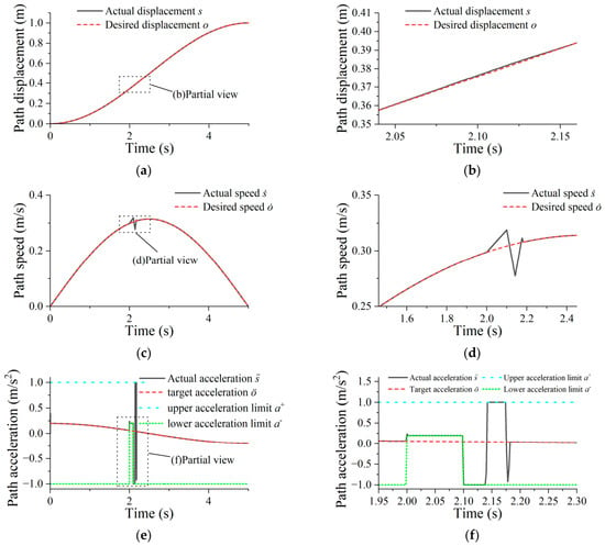
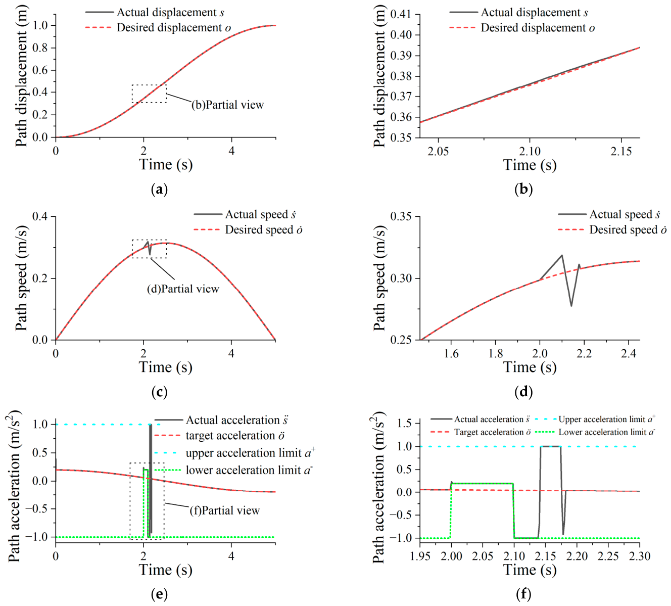
To verify the effectiveness of the improved nonlinear scaling filter under special acceleration bounds, a single-axis trajectory scaling test was first carried out. This test was designed to reproduce the boundary condition in which the lower acceleration bound becomes positive. In the conventional case, the acceleration bounds satisfy , and the trajectory scaling filter can directly generate a feasible acceleration command. However, after boundary modification, the lower acceleration bound was forced to become positive within a short time interval, resulting in . Under this condition, the path acceleration must remain positive, and the conventional scaling method may fail because its basic assumption on the acceleration bounds is no longer satisfied.
In the test, the reference trajectory, velocity bound, and upper acceleration bound were kept unchanged. Only the lower acceleration bound was modified during the selected interval to generate the same-sign acceleration-bound condition. The proposed boundary conversion method was then applied before the nonlinear scaling filter. The acceleration offset was calculated according to the current acceleration interval, and the converted acceleration bounds were used to compute the scaling command. After the filter output was obtained, the acceleration command was transformed back to the original path-parameter space and limited by the original physical bounds.
The comparison mainly includes the path response, velocity response, acceleration response, and local enlarged curves near the boundary-change interval. The results shown in Figure 3 show that the conventional scaling method may produce acceleration overshoot or local discontinuity when becomes positive. In contrast, the proposed method can keep the output acceleration within the feasible interval and maintain continuous path velocity. This confirms that the improved scaling filter can handle same-sign acceleration bounds and is suitable for the special boundary conditions caused by actuator constraint mapping.
Figure 3.
Single-axis trajectory scaling results under special acceleration bounds. (a) Path displacement comparison; (b) displacement comparison local magnification image; (c) path speed displacement comparison; (d) speed comparison local magnification image; (e) path acceleration comparison; (f) acceleration comparison local magnification image.
3.2. Experimental Verification of Velocity Scaling
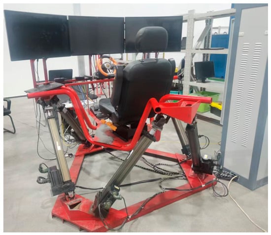
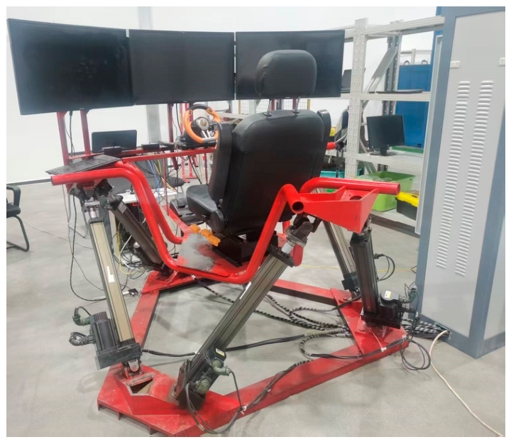
After the single-axis verification, the proposed condition-number-aware velocity bound regulation method was further tested on an electric-cylinder-driven Stewart experimental platform, as illustrated in Figure 4. The experimental system consists of a PC host, a Speedgoat real-time controller, Delta servo slaves, six electric-cylinder actuators, and the Stewart platform body. The geometric parameters of the platform were , , with short-side angular intervals of 15.7° and 14.0° for the base and moving platforms, respectively. The limb stroke range was , and the velocity and acceleration limits were and . The online planner was executed with a sampling period of . Two methods were compared: one without velocity boundary scaling, where , and the other with workspace-aware scaling based on the workspace region and dimensionless Jacobian condition number with , , , .
Figure 4.
The motion simulation platform.
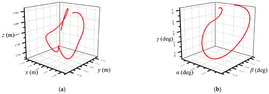
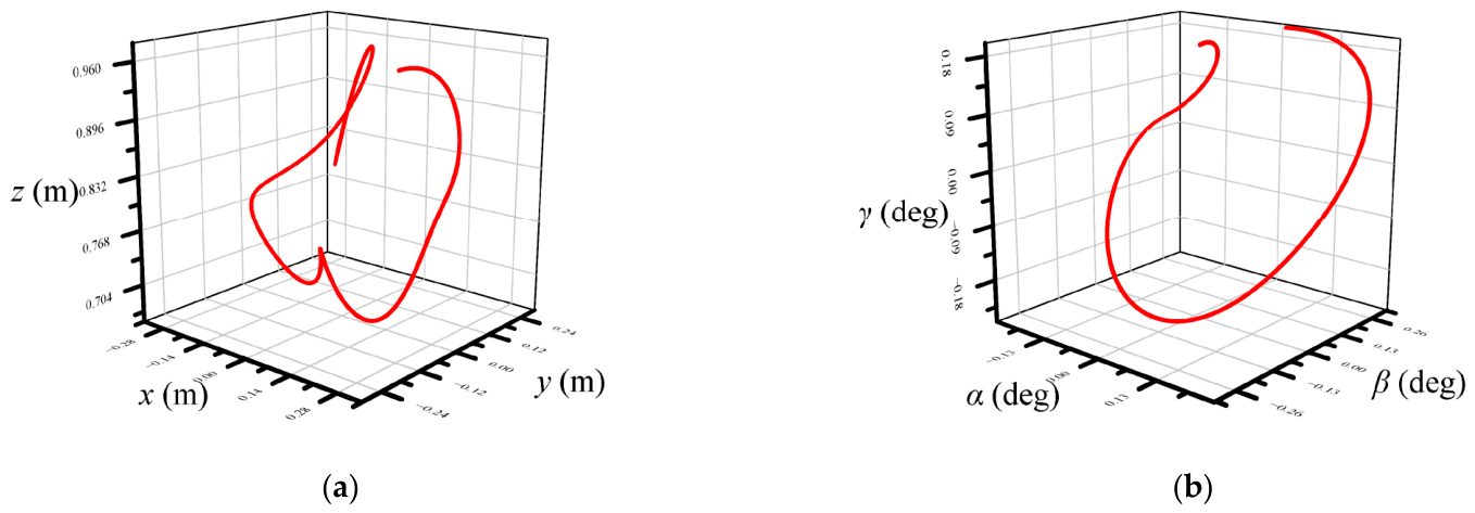
The experimental trajectory is shown in Figure 5. The reference path contains both translational and rotational components so that the platform passes through regions with different local motion capabilities. The selected trajectory was designed to pass from the rated workspace to the region with reduced motion capability.
Figure 5.
Experimental Path. (a) Experimental position; (b) experimental pose.
The path time law is defined as
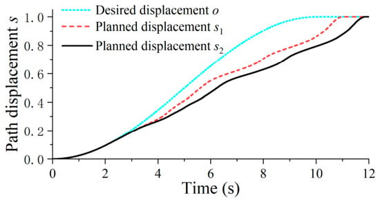
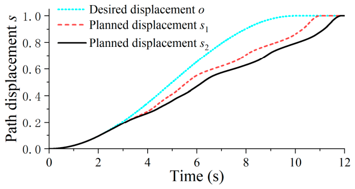
The optimized target path displacements obtained by the two methods are compared in Figure 6. Both planned curves try to track the desired displacement . However, when the platform moves away from the rated workspace, the local motion capability of the mechanism becomes limited, and the planned displacement cannot completely follow the desired displacement.
Figure 6.
Comparison of optimized target path displacements. The desired path displacement is denoted by , the planned displacement without velocity boundary scaling is denoted by , and the planned displacement with workspace-aware velocity scaling is denoted by .
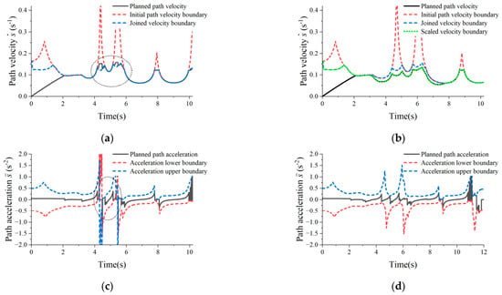
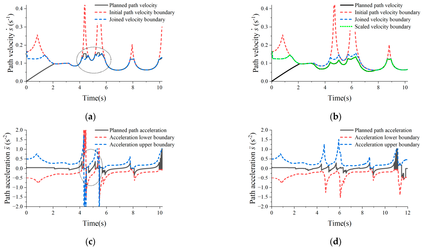
Compared with , the proposed method generates a more conservative planned displacement by reducing the velocity boundary according to the workspace state. To further explain this difference, the actuator velocities and accelerations are compared in Figure 7.
Figure 7.
Comparison of path velocity, path acceleration, and corresponding boundaries. (a) Path velocity without velocity boundary scaling; (b) path velocity with velocity boundary scaling; (c) path acceleration without velocity boundary scaling; (d) path acceleration with velocity boundary scaling.
Figure 7 compares path velocity, path acceleration and their respective boundaries for the two schemes. Without velocity scaling (Figure 7a,c), planned velocity converges to the combined velocity boundary within motion-limited regions. In the region outlined by dashed lines, an imminent velocity-bound violation compels the planner to tune path acceleration, which may yield infeasible acceleration ranges; path acceleration is thereby forced to zero to sustain planning, resulting in a local acceleration-constraint violation despite preserved velocity compliance. By contrast, with the proposed velocity scaling (Figure 7b,d), velocity limits are adaptively lowered based on workspace status and condition numbers when motion capacity is inadequate. Although slight local exceedances of the conservative scaled boundary can be observed, the joined boundary and acceleration feasibility are still maintained. Consequently, the presented approach mitigates acceleration-bound violation risks without degrading performance within feasible workspace areas.
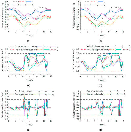
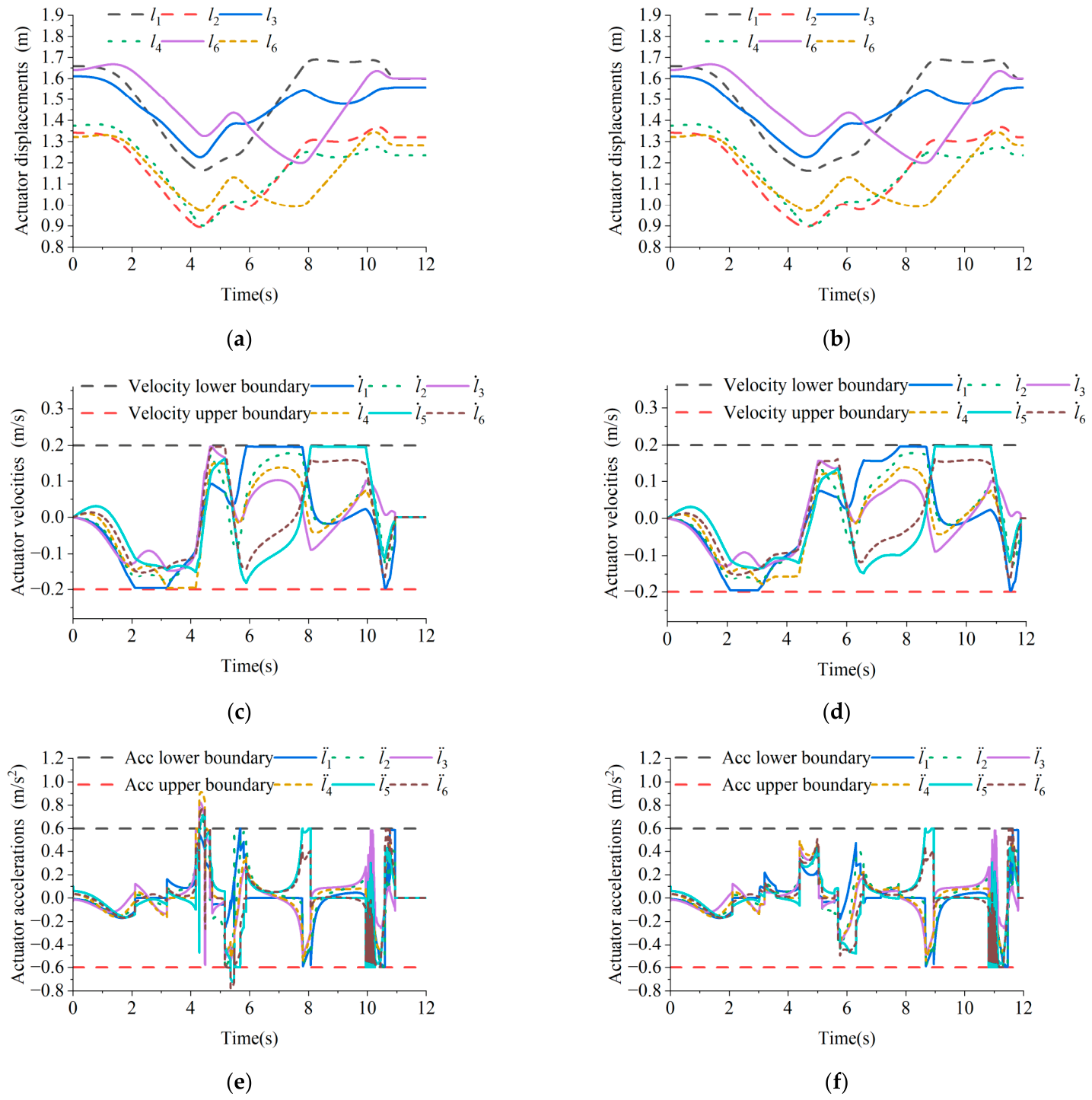
To further evaluate the influence of velocity scaling on actuator-level motion, the displacements, velocities, and accelerations of the six limbs are compared in Figure 8. Since the planned path is finally executed through the six electric-cylinder actuators, actuator responses can directly reflect whether the optimized path time law satisfies the physical motion constraints. As shown in Figure 8, after introducing the velocity scaling coefficient, the limb displacement curves remain continuous, while the actuator velocity and acceleration fluctuations are reduced. This indicates that the proposed method can improve actuator-level motion smoothness by regulating the path velocity boundary before the mechanism enters the region with limited motion capability.
Figure 8.
Comparison of actuator displacements, velocities, and accelerations with and without velocity scaling. (a) Actuator displacements without velocity boundary scaling; (b) actuator displacements with velocity boundary scaling; (c) actuator velocities without velocity boundary scaling; (d) actuator velocities with velocity boundary scaling; (e) actuator accelerations without velocity boundary scaling; (f) actuator accelerations with velocity boundary scaling.
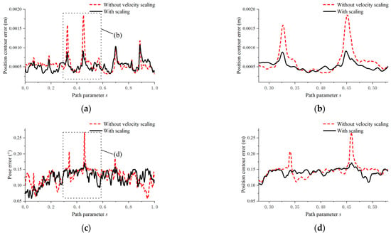
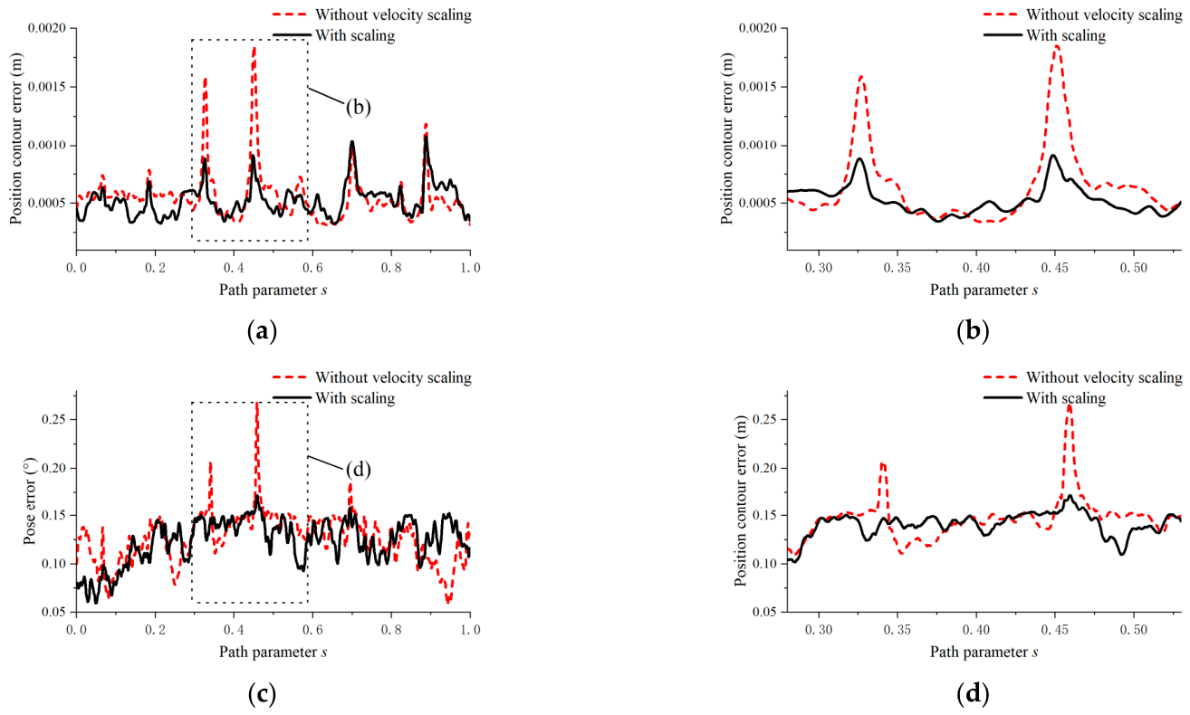
Due to the limited motion capability of the Stewart mechanism, the actual platform motion cannot completely track the desired trajectory when the platform moves away from the regions with sufficient local motion capability. In the regions, both methods can normally follow the target trajectory. Therefore, the comparison mainly focuses on the position contour error and pose error in the region with reduced motion capability.
The position contour error is defined as
where is the position vector, and is the actual position vector, is the reference position vector.
The pose error is defined as
where is the attitude vector, and is the actual attitude vector, is the reference attitude vector.
The comparison results are shown in Figure 9.
Figure 9.
Comparison of position contour error and pose error without and with velocity scaling. (a) Position contour error over the entire path; (b) enlarged view of the position contour error in the selected region; (c) pose error over the entire path; (d) enlarged view of the pose error in the selected region.
The mean value and standard deviation of the errors were further compared, as listed in Table 1. The mean value reflects the overall tracking accuracy, while the standard deviation reflects the fluctuation of the tracking error along the path. Since the two methods show similar tracking performance in most of the rated workspace, the statistical comparison was carried out over both the entire path and the selected boundary region.
Table 1.
Statistical comparison of position contour error and pose error over the entire path and selected boundary region.
For the entire path, the differences between the two methods are relatively limited, because both methods can normally track the target trajectory in the rated workspace. However, in the selected boundary region, the proposed method achieves lower mean errors and smaller error variances for both the position contour error and pose error. This indicates that the proposed scaling strategy mainly improves the tracking stability in the region with reduced motion capability while maintaining comparable performance in the normal workspace.
The statistical results in Table 1 further confirm the effectiveness of the proposed method. Over the entire path, the differences between the two methods are relatively small, because most of the trajectory is located in the rated workspace where the mechanism has sufficient motion capability. Nevertheless, the proposed method still reduces the mean position contour error by approximately 5.9% and the fluctuation of the position error by approximately 35.3%. The pose error also shows a slight decrease, indicating that the introduced velocity scaling does not degrade the overall tracking performance.
In the selected boundary region, the improvement becomes more significant. The mean position contour error is reduced by approximately 18.4%, and the fluctuation of the position error is reduced by approximately 63.1%. Meanwhile, the mean pose error is slightly reduced, and its fluctuation decreases by approximately 47.8%. These results indicate that the proposed velocity scaling mainly takes effect in regions with limited motion capability. By reducing the velocity boundary before the mechanism approaches the boundary region, the proposed method suppresses local error fluctuations and improves the stability of contour tracking.
4. Discussion
The experimental results demonstrate that the proposed method improves the feasibility and stability of online trajectory planning for the Stewart platform under limited motion capability. The single-axis test first verifies the effectiveness of the improved nonlinear scaling filter. When the lower acceleration bound becomes positive, the conventional assumption is no longer satisfied. In this case, the conventional scaling process may fail to generate a feasible acceleration command. By introducing the acceleration-bound conversion, the proposed method transforms the same-signed acceleration bounds into a regular form that can be handled by the nonlinear scaling filter. Therefore, the planned acceleration remains continuous and feasible under special boundary conditions.
In the Stewart platform experiment, the main challenge comes from the configuration-dependent motion capability of the mechanism. When the dimensionless Jacobian condition number increases, the local velocity transmission becomes less favorable, and the original joined velocity boundary may no longer provide sufficient safety margin. Without velocity scaling, the planned path velocity can approach or locally exceed the joined boundary, which may further lead to an infeasible acceleration interval and local acceleration-bound violation. By reducing the velocity boundary according to the condition number, the proposed method regulates the path time law before the mechanism reaches a low-mobility state.
The actuator-level results explain why the contour tracking performance is improved. Since the six electric-cylinder actuators are strongly coupled through the Stewart structure, excessive path velocity can be converted into large actuator velocity and acceleration fluctuations. The proposed scaling strategy suppresses these fluctuations by limiting the path velocity in advance. Therefore, the improvement is more evident in the boundary region or low-mobility configurations, while the difference over the entire path remains relatively small because both methods can track the target trajectory normally when the local motion capability is sufficient.
It should also be noted that the proposed method is not a global velocity reduction strategy. The original velocity boundary is preserved when the condition number indicates sufficient local motion capability, and the boundary is reduced only when performance degradation is detected. This makes the method more adaptive than directly applying a conservative global limit. However, its effectiveness depends on the accuracy of the Jacobian-based performance evaluation and the selected condition-number thresholds. Improper thresholds may lead to overly conservative or insufficient scaling. Future work will further incorporate dynamic constraints, load variation, and predictive optimization to improve adaptability under stronger disturbances and high-speed motion.
5. Conclusions
This paper proposed a condition-number-based velocity boundary scaling method for online trajectory planning of Stewart parallel mechanisms. The method combines path–velocity decomposition, actuator constraint mapping, nonlinear trajectory scaling, and Jacobian-based local performance evaluation. An acceleration-bound conversion strategy was also introduced to improve the nonlinear scaling filter under special acceleration bounds.
The single-axis test verified that the improved scaling filter can handle the case where the lower acceleration bound becomes positive. The experimental results on the electric-cylinder-driven Stewart platform further showed that the proposed velocity scaling method can reduce the path velocity boundary when the local motion capability degrades, thereby improving the feasibility of the planned trajectory and smoothing the actuator velocity and acceleration responses.
Quantitative contour error analysis showed that the proposed method mainly improves tracking stability in the boundary region. In the selected boundary region, the mean position contour error was reduced by approximately 18.4%, the fluctuation of the position error was reduced by approximately 63.1%, and the fluctuation of the pose error was reduced by approximately 47.8%. These results indicate that the proposed method can effectively improve online trajectory planning performance in configurations with limited motion capability while maintaining the geometric consistency of the target path.
Future work will further incorporate dynamic constraints, load variation, and predictive optimization into the proposed framework. This will improve the adaptability of the method under stronger disturbances, higher-speed motion, and more complex real-time tasks.
Author Contributions
Conceptualization, X.J.; Methodology, X.J., C.W. and L.Z.; Software, X.J.; Validation, X.J.; Formal analysis, X.J. and C.W.; Investigation, X.J. and H.Z.; Resources, X.J., H.Z. and B.Z.; Data curation, X.J., H.Z. and B.Z.; Writing—original draft, X.J.; Writing—review & editing, X.J.; Visualization, X.J.; Supervision, X.J.; Project administration, X.J. and L.Z.; Funding acquisition, L.Z. All authors have read and agreed to the published version of the manuscript.
Funding
This research was funded by National Natural Science Foundation of China No. 51875499; Natural Science Foundation of Hebei Province under Grant No. E2011203214.
Data Availability Statement
The data presented in this study are available on request from the corresponding author. The data are not publicly available due to the laboratory data management policy and the fact that part of the experimental data are related to the operation parameters of the self-developed experimental platform.
Conflicts of Interest
The authors declare no conflict of interest.
References
- Zhang, Z.; Meng, Q.; Cui, Z.; Yao, M.; Shao, Z.; Tao, B. Machine Learning Applications in Parallel Robots: A Brief Review. Machines 2025, 13, 19. [Google Scholar] [CrossRef] [Scilit]
- Zhang, T.; Cao, Y.; Ma, G. Trajectory planning of 3-CRU parallel robot with linear kinematics equation. Proc. Inst. Mech. Eng. Part C-J. Eng. Mech. Eng. Sci. 2022, 236, 9589–9609. [Google Scholar] [CrossRef] [Scilit]
- Wu, P.; Wang, Z.; Jing, H.; Zhao, P. Optimal Time-Jerk Trajectory Planning for Delta Parallel Robot Based on Improved Butterfly Optimization Algorithm. Appl. Sci. 2022, 12, 22. [Google Scholar] [CrossRef] [Scilit]
- Silva, D.; Garrido, J.; Riveiro, E. Stewart Platform Motion Control Automation with Industrial Resources to Perform Cycloidal and Oceanic Wave Trajectories. Machines 2022, 10, 28. [Google Scholar] [CrossRef] [Scilit]
- Zhao, S.; Gao, Z.; Meng, X.; Li, H. Multibody coupled dynamic response analysis of a dual barge float-over operation system with motion compensation equipment under a passive operational mode. Ocean Eng. 2023, 269, 14. [Google Scholar] [CrossRef] [Scilit]
- Shen, C.; Qu, H.; Guo, S.; Li, X. Kinematics Analysis and Singularity Avoidance of a Parallel Mechanism with Kinematic Redundancy. Chin. J. Mech. Eng. 2022, 35, 260–277. [Google Scholar] [CrossRef] [Scilit]
- Pham, Q.C.; Caron, S.; Lertkultanon, P.; Nakamura, Y. Planning Truly Dynamic Motions: Path-Velocity Decomposition Revisited. arXiv 2014, arXiv:1411.4045. [Google Scholar]
- Verscheure, D.; Demeulenaere, B.; Swevers, J.; De Schutter, J.; Diehl, M. Time-optimal path tracking for robots: A convex optimization approach. IEEE Trans. Autom. Control 2009, 54, 2318–2327. [Google Scholar] [CrossRef] [Scilit]
- Bobrow, J.E.; Dubowsky, S.; Gibson, J.S. Time-Optimal Control of Robotic Manipulators Along Specified Paths. Int. J. Robot. Res. 1985, 4, 3–17. [Google Scholar] [CrossRef] [Scilit]
- Pham, H.; Pham, Q. A New Approach to Time-Optimal Path Parameterization Based on Reachability Analysis. IEEE Trans. Robot. 2018, 34, 645–659. [Google Scholar] [CrossRef] [Scilit]
- Shin, K.G.; Mckay, N.D. Selection of Near-Minimum Time Geometric Paths for Robotic Manipulators. IEEE Trans. Autom. Control 1986, 31, 501–511. [Google Scholar] [CrossRef] [Scilit]
- Pham, Q.-C. A general, fast, and robust implementation of the time-optimal path parameterization algorithm. IEEE Trans. Robot. 2014, 30, 1533–1540. [Google Scholar] [CrossRef] [Scilit]
- Zanasi, R.; Bianco, C.G.L.; Tonielli, A. Nonlinear filters for the generation of smooth trajectories. Automatica 2000, 36, 439–448. [Google Scholar] [CrossRef] [Scilit]
- Gerelli, O.; Bianco, C.G.L. Nonlinear variable structure filter for the online trajectory scaling. IEEE Trans. Ind. Electron. 2009, 56, 3921–3930. [Google Scholar] [CrossRef] [Scilit]
- Gerelli, O.; Bianco, C.G.L. A discrete-time filter for the on-line generation of trajectories with bounded velocity, acceleration, and jerk. In Proceedings of the 2010 IEEE International Conference on Robotics and Automation, Anchorage, AK, USA, 3–7 May 2010. [Google Scholar]
- Bianco, C.G.L.; Ghilardelli, F. A scaling algorithm for the generation of jerk-limited trajectories in the operational space. Robot. Comput. Integr. Manuf. Int. J. Manuf. Prod. Process Dev. 2017, 44, 284–295. [Google Scholar] [CrossRef] [Scilit]
- Yuan, M.; Chen, Z.; Yao, B.; Hu, J. An Improved Online Trajectory Planner With Stability-Guaranteed Critical Test Curve Algorithm for Generalized Parametric Constraints. IEEE/ASME Trans. Mechatron. 2018, 23, 2459–2469. [Google Scholar] [CrossRef] [Scilit]
- Shen, P.; Zhang, X.; Fang, Y.; Yuan, M. Real-Time Acceleration-Continuous Path-Constrained Trajectory Planning With Built-In Tradeoff Between Cruise and Time-Optimal Motions. IEEE Trans. Autom. Sci. Eng. 2020, 17, 1911–1924. [Google Scholar] [CrossRef] [Scilit]
- Zhang, S.; Li, W.; Zhou, S.; Angeles, J.; Chen, W.; Gao, F.; Guo, W. Kinematics and workspace analysis of a 3-CR(Pa)(Pa)R parallel mechanism with an orthogonal layout. Mech. Mach. Theory 2024, 195, 105616. [Google Scholar] [CrossRef] [Scilit]
- Gosselin, C.; Angeles, J. Singularity analysis of closed-loop kinematic chains. IEEE Trans. Robot. Autom. 2002, 6, 281–290. [Google Scholar]

Disclaimer/Publisher’s Note: The statements, opinions and data contained in all publications are solely those of the individual author(s) and contributor(s) and not of MDPI and/or the editor(s). MDPI and/or the editor(s) disclaim responsibility for any injury to people or property resulting from any ideas, methods, instructions or products referred to in the content. |
© 2026 by the authors. Licensee MDPI, Basel, Switzerland. This article is an open access article distributed under the terms and conditions of the Creative Commons Attribution (CC BY) license.