


Abstract
The groove curvature coefficient plays a critical role in determining the thermo-mechanical performance of angular-contact ball bearings. However, its optimization remains challenging due to strong nonlinear coupling among stress, stiffness, heat generation, and fatigue capacity. To address this issue, this study proposes a hybrid optimization framework integrating a corrected two-dimensional axisymmetric finite element method (2D-AxFEM) model, a deep learning surrogate model, and a genetic algorithm. Firstly, an efficient 2D-AxFEM model calibrated by a bearing dynamic model is developed to accurately predict key performance metrics, including contact stress, stiffness, heat generation, and dynamic load rating, with significantly reduced computational cost compared to the conventional 3D FEM model. Based on the generated data, a multi-layer perceptron deep learning surrogate model is trained to establish a fast nonlinear mapping between groove curvature coefficients and performance indicators. The model achieves high accuracy, with R2 values of 0.9745, 0.9414, and 0.9756 at three different rotational speeds, as well as significantly improved computational efficiency. Building upon this, single- and multi-constraint optimization problems are solved using a genetic algorithm. The results reveal clear trade-offs among stiffness, heat generation, and load capacity. Under stiffness constraints, optimal solutions consistently converge to the constraint boundary, indicating its dominant role in thermal optimization. Under multiple constraints, the framework effectively identifies feasible design regions, enabling reduced heat generation while maintaining acceptable stress and load capacity. Overall, the proposed framework enables efficient exploration of multi-physics design spaces and provides a scalable solution for high-speed bearing optimization.
1. Introduction
High-speed precision rolling bearings are essential components in advanced mechanical systems such as aero-engines, machine tool spindles, and high-speed railways. Their performance directly governs the rotational accuracy, service life, and reliability of the entire system [1,2,3]. Among various design parameters, the groove curvature coefficient plays a decisive role in determining contact mechanics, load distribution, and thermo-mechanical behavior under high-speed conditions [4]. However, its influence exhibits strong nonlinearity and inherent trade-offs. For instance, a smaller curvature coefficient improves stiffness and reduces contact stress, yet significantly increases frictional heat generation, thereby elevating the risk of thermal failure [5,6]. This multi-physics coupling poses substantial challenges for optimal bearing design.
In the realm of bearing parametric design and performance analysis, analytical methods are widely employed, primarily encompassing quasi-static and dynamic models. These analytical models focus on solving the nonlinear systems derived from geometric relationships and force equilibrium under high-speed conditions [7,8].
The classic quasi-static model was proposed by Jones [9,10] in 1959. Noel et al. [11] employed the quasi-static model to develop a method for calculating the stiffness matrix. Yang et al. [12] analyzed the effects of different preloads, rotational speeds, and structural parameters on bearing stiffness. However, the quasi-static model only considers the equilibrium state under bearing load and neglects high-speed dynamic effects such as spin and sliding, which are of considerable importance to bearing behavior. When calculating fatigue loads, Pape et al. [13] took into account the influence of spin and sliding on stress. With advances in elastohydrodynamic lubrication (EHL) theory, bearing dynamic models can now not only capture the effects of high-speed spin and sliding on the contact zone, but also compute interactions among multiple components. He et al. [14] constructed a high-speed bearing dynamic model, simulating the six-degree-of-freedom motion of the balls and cage and the five-degree-of-freedom motion of the rings, and calculated dynamic characteristic parameters such as the spin-to-roll ratio and slip velocity. Wen et al. [15] used a dynamic model to specifically investigate the misalignment of high-speed miniature ball bearings, finding that misalignment leads to an increase in spin friction torque. Ma et al. [16] proposed a nonlinear dynamic model for four-point-contact ball bearings and provided strategies to reduce sliding damage. Liu et al. [17] established a dynamic model incorporating temperature and lubricant effects, revealing the significant influence of lubricant temperature on ball skidding behavior. Although the aforementioned dynamic models provide valuable physical insights, they not only face notable computational efficiency challenges when solving the differential equations of motion, but also struggle to effectively address flexibility-related bearing nonlinearity problems.
With the advancement of computational mechanics, the finite element method (FEM) has emerged as a robust tool for high-fidelity bearing performance analysis [18]. He et al. [19] established an integrated bearing-bolt FEM model, and Guo et al. [20] investigated cross-coupling stiffness characteristics using FEM/contact mechanics approaches. Zhang et al. [18] applied FEM modeling combined with minimum potential energy principles to evaluate stiffness in rotor systems. Nevertheless, high-fidelity 3D-FEM models are prohibitively expensive in terms of computational cost, making them impractical for large-scale parameter sweeps and iterative optimization [21]. Therefore, a key challenge lies in developing an efficient yet sufficiently accurate modeling approach that can support large-scale design exploration.
In recent years, deep learning methods have demonstrated strong capability in modeling complex nonlinear relationships in mechanical design, particularly for performance prediction tasks [22,23,24,25]. For instance, Ji et al. [26] applied machine learning models to predict bearing temperature, while Gheller et al. [27] employed artificial neural networks (ANNs) to estimate lubrication-related parameters with high efficiency. In addition, Wang et al. [28] developed a machine learning-based surrogate model for friction prediction in textured journal bearings, achieving high accuracy while significantly reducing the computational cost associated with simulations. Zhao et al. [29] used deep neural networks (DNN) to construct reduced-order models for tilting pad journal bearings, enabling accurate prediction of stiffness, damping, and thermal behavior with orders-of-magnitude improvement in efficiency. These studies demonstrate the effectiveness of deep learning as a predictive tool for complex multi-physics mechanical systems.
Building upon this, surrogate-based optimization frameworks have been developed by coupling deep learning models with intelligent optimization algorithms. In such frameworks, the trained surrogate model replaces expensive numerical simulations, enabling rapid evaluation during iterative optimization. For example, Baklouti et al. [30] and Gao et al. [31] integrated surrogate models with optimization algorithms to improve bearing performance. Furthermore, Zhao et al. [32] proposed a hybrid framework combining thermal networks and machine learning for joint optimization. In addition, Ganesha et al. [33] applied data-driven optimization strategies to advanced bearing configurations, where machine learning models are combined with optimization algorithms to identify optimal structural parameters. Beyond conventional surrogate-based approaches, Kim et al. [34] introduced deep reinforcement learning (DRL) for bearing design, enabling adaptive optimization under varying operating conditions and improving design flexibility. Furthermore, Liu et al. [35] explored hybrid strategies combining deep learning with evolutionary algorithms to enhance convergence efficiency and global search capability in air-bearing design problems. Despite these advancements, the distinction between single-constraint and multi-constraint optimization, as well as their impact on optimal design evolution, remains largely unexplored. This gap limits the applicability of existing methods to realistic engineering scenarios involving strict design requirements.
Accordingly, this paper introduces a comprehensive design framework that integrates an efficient 2D axisymmetric finite element method (2D-AxFEM) model, deep learning surrogate modeling, and intelligent optimization algorithms, as illustrated in Figure 1. First, an efficient 2D-AxFEM model corrected by the dynamic model is employed to rapidly obtain critical performance metrics, including stiffness, contact stress, heat generation rate, and dynamic load rating under varying groove curvature coefficients, significantly reducing the computational cost while maintaining accuracy. Subsequently, a high-precision deep learning surrogate model is trained to establish fast mapping from design parameters to multiple performance indicators. Finally, leveraging this deep learning surrogate model, both single-constraint optimization and multi-constraint optimization are systematically conducted for rotational speeds of 10,000, 20,000, and 30,000 rpm. This framework enables efficient exploration of constrained design spaces and reveals the evolution patterns of optimal groove curvature coefficients under multiple operating conditions, providing a practical and scalable solution for high-speed bearing optimization.
Figure 1.
Optimization framework for high-speed precision bearings.
2. 2D-Axisymmetric FEM Model and Performance Metrics
2.1. 2D-Axisymmetric FEM Model of Bearing
This paper takes the type 7008C angular-contact ball bearing as the research object for analysis, as shown in Figure 2, with its structural parameters listed in Table 1. An efficient and high-fidelity finite element method (FEM) model is indispensable for the design optimization of bearings. However, full three-dimensional (3D) FEM models are often plagued by prohibitively low computational efficiency. This inefficiency stems not only from excessive mesh counts and the necessity of solving massive systems of nonlinear equations, but also from complex nonlinear behaviors—such as frictional contact and separation—which frequently lead to convergence difficulties. Consequently, utilizing full 3D-FEM models is impractical for efficient large-scale batch simulations and analysis.
Figure 2.
7008C angular-contact ball bearing. (a) Photograph of the bearing. (b) Cross-sectional view and dimensional annotation.
Table 1.
Structure parameters of bearing.
To achieve a balance between efficiency and accuracy, the high-speed rolling elements are simplified as equivalent annular components, leveraging their characteristic of positional uncertainty under high rotational speeds. Specifically, under the condition of steady operation at high rotational speed, the rolling elements of the angular-contact ball bearing are distributed regularly in the circumferential direction. Their motion state has strict periodicity and symmetry characteristics in a statistical sense. Based on this physical property, the discrete distribution of multiple rolling elements can be equivalently regarded as a continuous virtual annular structure, as shown in Figure 3. This equivalent ring is conceptually composed of infinite virtual rolling elements continuously, and its equivalent material parameters can be systematically calibrated through the bearing dynamics theoretical model, thereby ensuring that this equivalent structure can accurately reflect the macroscopic mechanical behavior of the bearing under different working conditions [21,36]. In Section 2.2, the strict equivalence of the 2D-AxFEM model using bearing dynamics will be elaborated upon in detail. Upon correction via the bearing dynamic analytical model, the 2D-AxFEM model facilitates the precise computation of critical performance metrics (stiffness and maximum contact stress) under high-speed operation.
Figure 3.
Schematic illustration of the bearing simplification approach. (a) Actual bearing model. (b) Simplified model for high-speed analysis. (c) Cross-section of the simplified bearing.
Following this simplification, the bearing assembly, consisting entirely of annular structures, can be simulated using the 2D axisymmetric finite element method. This section will describe the process of constructing the 2D-AxFEM model.
A 2D-AxFEM model of the bearing was constructed using the finite element simulation software ABAQUS-6.14. In the cylindrical coordinate system , the geometric equations representing the strain–displacement relationship are given by Equation (1). Furthermore, the weighted integration is calculated via Equation (2) [37,38,39].
The equilibrium equations are governed by Equation (3). denotes the stress field and represents the body force vector.
The constitutive equations are given by Equations (4) and (5), with representing the elastic stiffness matrix.
The model is discretized using 4-node linear axisymmetric reduced-integration elements (CAX4R). As defined in Equation (6), the shape functions utilize bilinear interpolation to govern the intra-element displacement field, thereby enabling the calculation of displacements at any arbitrary point based on nodal values.
Subsequently, applying the principle of virtual work yields the element stiffness matrix, as presented in Equation (7).
The global governing equations of the system are derived by assembling the individual element stiffness matrices, as presented in Equation (8).
The ABAQUS/Standard solver employs an implicit integration scheme to solve these equations, thereby yielding the nodal displacements and stress fields.
To balance computational efficiency with numerical accuracy, a mesh independence study was conducted. Six different global coarse-to-local refined mesh sizes were adopted, as shown in Table 2. By comparing the key output quantities under different sizes, the sensitivity to mesh size was evaluated (the equivalent calculation method for the key output quantity will be elaborated upon in Section 2.2). The results indicated that when the global element size was 0.5 mm and the local refined mesh size was 0.005 mm, the calculation results tended to be stable. Further mesh refinement resulted in limited improvement in accuracy but significantly increased the computational cost. Therefore, a global mesh size of 0.5 mm and a local mesh size of 0.005 mm were determined to be the optimal sizes, effectively controlling the computational scale while ensuring numerical accuracy. The final generated finite element model contained 8347 nodes and 8017 elements, and the meshing results are shown in Figure 4.
Table 2.
Verification results of the mesh independence of the 2D-AxFEM model.
Figure 4.
Illustration of the 2D-AxFEM model. (a) Model configuration. (b) Mesh discretization results.
The contact between each component of the bearing is set as general contact, with normal hard contact and tangential Coulomb friction. The bearing is lubricated with grease, and the friction coefficient is set to 0.001. This coefficient is calculated using Equation (9), where represents the sliding velocity, and A, B, C, and D are coefficients related to the contact and lubrication conditions within the sliding contact zone. The aforementioned coefficients can be determined from the dynamic model presented in Section 2.2.1 [40].
Since this model is an axisymmetric model, no additional boundary conditions or loads need to be set in the radial direction. In the axial direction, a fixed outer ring at the upper end is used, and axial loading (500 N) is applied at the lower end of the inner ring to impose constraints.
The inner and outer rings of the bearing are both continuous and uniform solid structures with consistent material properties. The material parameters used are for GCr15 bearing steel (elastic modulus E = 208 GPa, Poisson’s ratio ν = 0.3) to truly reflect its elastic deformation behavior under load. The rolling elements have been simplified as axisymmetric equivalents based on their position uncertainty characteristics under high-speed rotation. Therefore, the material properties of these elements also require strict equivalent calculations, which are described in detail in Section 2.2.
2.2. Bearing Dynamic Model and Equivalence Method
To ensure the 2D-AxFEM model accurately represents the bearing state under varying rotational speeds, the equivalent elastic modulus and Poisson’s ratio of the rolling elements are modified to capture the stiffness variations associated with high-speed rotation. Simultaneously, the contact stress formulation within the 2D-AxFEM is calibrated to account for centrifugal effects. Consequently, a bearing dynamic model is utilized to determine the equivalent high-speed stiffness and contact stress parameters, enabling the 2D-AxFEM to predict performance variations under diverse speed and load conditions.
2.2.1. Bearing Dynamic Model
The dynamic model is established by analyzing the kinematic behaviors of individual bearing components and the complex forces arising from their interactions. Specifically, the governing dynamic differential equations are derived by rigorously analyzing the local forces and kinematic relationships within three key subsystems: ball-to-cage interactions, ball-to-groove interactions, and cage-to-guide-ring interactions [40,41].
For a component with six degrees of freedom, its motion state is determined by three translational degrees of freedom and three rotational degrees of freedom. According to Newton’s second law, the differential equations of motion for each component in the system can be established [42]. Considering the distinct characteristics of different components’ motion patterns, the equations of motion for rolling elements are formulated in an inertial cylindrical coordinate system, while those for the inner ring and the cage are described in an inertial Cartesian coordinate system, as shown in Figure 5a. is the inertial coordinate system, is the rolling element coordinate system, and is the inner-raceway coordinate system. In the contact analysis between the ball and the raceway, a contact coordinate system and an elastohydrodynamic lubrication coordinate system are defined. In Figure 5a, B denotes the center of mass of the rolling element, and represent the center of mass and geometric center of the inner raceway, respectively, and is the arc center of the raceway. The vector denotes the position vector from the raceway arc center to point B, where the superscript indicates the coordinate system in which the vector is expressed. The vector denotes the vector from the raceway geometric center to point B. These two vectors can be expressed by the following equations:
Figure 5.
Geometric relationship and coordinate system of the ball and raceway. (a) Vector relationship and coordinate system. (b) Flowing particle coordinate system and contact area coordinate system.
Let and denote the resultant forces acting on the component in the inertial coordinate system, respectively. Then the equations of motion can be expressed as:
In cylindrical coordinates, the equations are expressed as:
The rotational motion of the component satisfies Euler’s equations of motion:
where represents the angular velocity vector of the component, and represents the angular acceleration vector; the subscripts 1, 2, and 3 correspond to the components along the directions of the body-fixed coordinate system, respectively. For the rolling element, the position, velocity, and acceleration of its center of mass in the cylindrical coordinate system are denoted by , and , respectively. For the cage and the inner ring, the motion states of their centers of mass in the Cartesian coordinate system are represented by , and , respectively.
Figure 5b shows the relative orientation between the contact coordinate system and the elastohydrodynamic lubrication coordinate system. For the inner-ring contact zone, and are opposite in direction, and are opposite in direction, and and are opposite in direction. For the outer-ring contact zone, and are opposite in direction, whereas and share the same direction, and and also share the same direction.
Based on the point-contact elastohydrodynamic lubrication (EHL) theoretical model [43,44,45,46], EHL modeling is performed for the ball–raceway contact zones [42]. In addition to the velocity in the rolling direction, gyroscopic sliding perpendicular to the rolling direction and spin motion also exist in the ball–raceway contact zone. Considering the two-directional sliding, the spin effect, the thermal effect, and the non-Newtonian behavior of the lubricant, the generalized Reynolds equation can be written in the following form [47]:
where is the lubricant viscosity, is the lubricant density, is the pressure, and is the oil film thickness.
The film thickness equation is:
The lubrication energy equation is:
The Newtonian viscosity of the fluid is calculated using the Roelands formula [42]:
The relationship between lubricating oil density and both temperature and pressure is given by the Dowson–Higginson formula [42]:
At any point within the contact region, the velocities of the rolling element and the raceway surface can be expressed as:
where the velocity of the raceway surface is
where the velocity of the rolling element surface is:
The spin moment generated by the shear stress within the contact region can be expressed as:
where and denote the spin moments about the -axis and -axis, respectively; and are the shear stresses acting on the rolling element surface. The spin angular velocity of the contact region induced by the rotation of the rolling element can be expressed as:
Within the contact region, the force vector (consisting of the contact force and friction force) and the moment vector can be expressed by Equation (25).
Figure 6 shows the geometric relationship between the cage and the outer-ring guide surface. In Figure 6, denotes the cage coordinate system. The oil film thickness between the cage and the outer-ring guide surface can be expressed as:
where can be calculated as follows:
where is the radius of the outer-ring guide surface, and is the coordinate transformation matrix from the cage coordinate system to the inertial coordinate system.
Figure 6.
Geometric relationship between the cage and the outer ring.
Based on the fluid pressure distribution, the resultant force and moment acting on the cage can be obtained:
where denotes the shear stress along the circumferential direction.
The spatial relationship between the rolling element and the cage pocket is shown in Figure 7. In the figure, denotes the center position of the pocket, is the pocket radius, and is the local coordinate system established at the pocket center. Based on this coordinate system, the relative motion between the rolling element and the cage can be described.
Figure 7.
Geometric relationship between the ball and the cage.
The local clearance between the rolling element and the pocket can be expressed by Equation (30).
The surface velocity induced by the rotation of the rolling element is:
After obtaining the distributions of the lubricant pressure and shear stress, the interaction forces between the rolling element and the cage can be calculated through integration.
where and denote the shear stresses on the surface in the and directions, respectively. From the aforementioned forces, the moment between the rolling element and the cage can be further obtained, and its expression is
Based on the interaction forces and moments among the aforementioned components, the accelerations and angular accelerations of each component are obtained. Substituting these into Equations (11)–(13) yields the differential equations of dynamic motion. The Runge–Kutta method is employed to solve the established system of dynamic equilibrium equations, thereby obtaining critical state parameters—such as displacements, velocities, and contact forces—for the bearing components under high-speed conditions. Subsequently, the results derived from this dynamic model serve as the basis for correcting the 2D-AxFEM model [21,36].
2.2.2. 2D-AxFEM Model
The transient dynamic model allows for the calculation of force and displacement curves for the bearing under varying rotational speeds, as expressed in Equation (35).
Using the 2D-AxFEM model of the bearing, force and displacement curves are calculated for various values of and . These relationships are mathematically represented in Equation (36):
To identify the optimal equivalent parameters, the maximum stiffness error is defined as the objective function. Specifically, this entails searching for the parameter combination that minimizes the discrepancy between the stiffness calculated by the 2D-AxFEM model and the theoretical dynamic stiffness:
where , , , and Solving this optimization problem yields the optimal and needed for accurate stiffness prediction at specific speeds. The calculation results are shown in Table 3.
Table 3.
Equivalent material constitutive parameters corresponding to different rotational speeds.
Table 3 presents the equivalent material parameters of the rolling elements under different rotational speeds. In essence, the variation in these equivalent parameters with rotational speed reflects the influence of rotational speed on bearing stiffness. When the bearing operates at high speed, the centrifugal force acting on the rolling elements becomes significant. This centrifugal force alters the displacement and geometric relationships between the rolling elements and the inner/outer raceways, leading to a new equilibrium state. Consequently, the bearing stiffness undergoes notable changes with rotational speed. Furthermore, this trend is generally applicable to other types of angular-contact ball bearings. Under high-speed rotation, the centrifugal force on the rolling elements is substantial. Within the contact region with the raceways, this centrifugal force is resolved into axial and radial components, which fundamentally modify the internal contact state. When an external load is applied, it can partially counteract the effect of the centrifugal force, manifesting as a reduction in the effective bearing stiffness.
When the equivalent rolling elements use the equivalent material parameters listed in Table 3, the force and displacement curves calculated by the 2D-AxFEM model of the bearing can be made consistent with the calculation results of the dynamic model.
In this way, the accurate stiffness value can be calculated. The specific calculation method is as follows: for the outer ring of the fixed bearing, apply an axial force to the inner ring of the bearing, extract the displacement change in the inner ring of the bearing, and compare it with the axial force. Thus, the stiffness of the bearing can be obtained, as shown in Equation (38).
To verify the accuracy of this method, the force and displacement curves of the bearing in a stationary state were measured using a bearing protrusion measurement instrument. These results were compared with the simulation calculations of the 2D-AxFEM model. The comparison results are shown in Figure 8. It should be noted that accurately and stably measuring the force–displacement curves of bearings under high-speed rotation remains a significant technical challenge due to limitations in current measurement instrumentation and test rig capabilities. Consequently, at this stage, the feasibility of the proposed method is validated only using experimentally obtained force–displacement curves under stationary (quasi-static) conditions. For subsequent analyses, the results at high rotational speeds are taken as those computed by the analytical dynamic model, which serves as the reference standard. This approach is consistent with common practice in bearing research where direct high-speed experimental validation is not yet feasible.
Figure 8.
Comparison between simulation and experiment of 2D-AxFEM. (a) Bearing protrusion measurement instrument. (b) Comparison results of experiment and simulation.
Figure 8 shows that by using the 2D-AxFEM model of the bearing with the rolling element constitutive behavior equivalent, the simulation calculation results of force and displacement curves are compared with the experimental results, and the error is less than 1 μm. The accuracy of the 2D-AxFEM model has been effectively verified.
Further, due to the geometric simplification in the 2D-AxFEM model, direct extraction of Hertzian contact stress is not feasible. To address this, a mapping correction approach based on the dynamic model is implemented. The contact stress (CPRESS) is modeled as a function of preload and speed (see Equation (39)), with the specific relationship derived via fitting calculations from the dynamic model.
Solving the bearing dynamic model yields the maximum contact stress results under various rotational speeds and load conditions. Based on these results, the maximum contact stress is initially fitted as a polynomial function of the preload force, as expressed in Equation (40). The coefficients within this function are dependent on velocity ; these parameters are determined through a secondary polynomial fitting with respect to speed, as shown in Equation (41).
The aforementioned fitting formulas enable the calculation of maximum contact stress within the 2D-AxFEM model under varying load and speed conditions. Using the formulas obtained through fitting, the maximum contact stresses of the inner and outer rings of the bearing at rotational speeds of 10,000, 20,000, and 30,000 rpm were calculated and compared with the calculation results of the dynamic model. The comparison results are shown in Figure 9. Figure 9 shows that after the 2D-AxFEM model is corrected by the fitting formula, the accurate maximum contact stress of the bearing can be calculated.
Figure 9.
Comparison of the calculated and fitting results of the maximum contact stress at different speeds. (a) Inner-ring results. (b) Outer-ring results.
In summary, the 2D-AxFEM model corrected by the dynamic model can accurately calculate the stiffness and contact stress of the bearing. The essence of the 2D-AxFEM model lies in mapping the high-speed mechanical response of the bearing dynamic model into the 2D-AxFEM model through equivalent material constitutive relations and contact stress calculation methods. This model not only retains the capability of the finite element method to address nonlinear problems, but also fully leverages the advantages of the bearing dynamic model in calculating high-speed characteristics.
To verify the computational efficiency advantage of the proposed 2D-AxFEM, a benchmark study was carried out comparing it against a conventional 3D FEM. Consistent loading conditions and material properties were adopted for both approaches, and grids with similar element sizes were generated. Parallel computation was enabled for both models using eight processors. To eliminate hardware-related discrepancies, all simulations were executed on a unified workstation featuring an Intel Xeon Platinum 8260 CPU (48 cores, 48 threads), 128 GB DDR4 memory, and an NVIDIA T1000 GPU (for hybrid acceleration), operating at a base frequency of 2.4 GHz.
Table 4 compares the 2D-AxFEM and the 3D FEM in terms of the number of nodes, number of elements, computation time, and key computational results. The results show that, under the same minimum mesh size, the 2D-AxFEM requires significantly fewer elements and nodes than the 3D FEM. Compared with the 3D FEM, the 2D-AxFEM achieves a computational error of only 8.5%, while improving computational efficiency by a factor of 12.4. This advantage is crucial for subsequent batch computations and optimization tasks.
Table 4.
Comparison of computational efficiency and errors between 2D-AxFEM and 3D-FEM models of bearings.
Therefore, this study adopts an orthogonal modeling approach based on the 2D-AxFEM model to establish bearing models with inner-ring coefficients ranging from 0.51 to 0.58 and outer-ring coefficients ranging from 0.51 to 0.58, resulting in a total of 64 different structural parameters. Three rotational speed conditions (10,000, 20,000, and 30,000 rpm) are also set. Finally, 192 models are calculated. Based on the boundary conditions described in Section 2.1, simulation analyses are performed, and the results are extracted to obtain the stiffness and maximum contact stress data for different bearing structures and rotational speeds.
2.3. Heat Generation Rate of the Bearing
The coupled 2D-AxFEM and dynamic model enables the calculation of critical parameters, such as velocity and stress, under high-speed rotation. Based on these parameters, the heat generation rate is determined using established thermal formulations. According to the Harris heat generation model [48,49], the thermal load in high-speed bearings primarily originates from four sources:
(1) Sliding friction at the rolling element–groove interface; (2) viscous friction caused by lubricant drag; (3) spin friction of the rolling elements induced by gyroscopic moments; (4) sliding friction between the cage and the ring-guiding surfaces.
(1) Sliding friction at the rolling element–groove interface
During high-speed operation, the combined effect of contact forces and high sliding velocities within the contact zone results in significant frictional heat generation between the rolling elements and the grooves. This heat generation is quantified by evaluating the thermal contributions at individual integration points along the and directions. Taking the -direction as an example, the heat generated in the contact zone is calculated using Equation (42). Here, denotes the frictional shear stress in the -direction, represents the sliding velocity, represents the contact patch area formed under the consideration of local slip phenomena, and indicates the contact area.
Similarly, the heat generation along the -direction can also be calculated. Thus, the total heat generated by sliding friction can be expressed by Equation (45).
(2) Viscous friction caused by lubricant drag
Under high-speed operating conditions, the interaction between the rolling elements and the lubricant produces viscous drag. This resistance leads to viscous friction heat, which is calculated by Equation (46).
Here, denotes the lubricant drag force, represents the orbital speed of the rolling elements, is the bearing pitch diameter, is the effective fluid density, is the drag coefficient, and is the diameter of the rolling element.
(3) Spin friction of the rolling elements induced by gyroscopic moments
During high-speed operation, the moment induced by the gyroscopic effect causes the rolling elements to spin about their own axes, generating substantial heat in the contact zone. The resulting spin friction heat can be calculated using Equation (48), where is the spin angular velocity of the rolling element and is the spin friction moment. In Equation (49), denotes the normal contact force between the inner groove and the rolling element, while represents the elliptic integral of the second kind for the contact ellipse.
(4) Sliding friction between the cage and the ring-guiding surfaces
During high-speed rotation, friction heat is also generated between the cage and the ring-guiding surfaces. This portion of heat can be calculated using Equation (50).
where represents the sliding friction force, is the diameter of the cage guiding surface, denotes the dynamic viscosity of the lubricant, indicates the rotational speed of the cage, and is the rotational speed of the ring.
In summary, the total heat generation rate of the bearing under high-speed rotation can be obtained through Equation (52).
Based on the above method, the heat generation rates are calculated for bearings with inner and outer-ring coefficients ranging from 0.51 to 0.58 at rotational speeds of 10,000, 20,000, and 30,000 rpm. These results serve as key indicators for evaluating the heat generation performance of the bearings.
2.4. Basic Dynamic Load Rating
The basic dynamic load rating is a key indicator for assessing the anti-fatigue load-carrying capacity of angular-contact ball bearings, and directly reflects the fatigue life of the bearing. It is defined as the maximum load that a bearing can withstand after one million revolutions. A larger basic dynamic load rating corresponds to a longer fatigue life of the bearing. The groove curvature coefficient is the primary factor influencing the basic dynamic load rating of the bearing. The formula for calculating the basic dynamic load rating is given as follows [49]:
where denotes the basic dynamic load coefficient related to material properties, represents the basic dynamic load coefficient associated with the internal geometry, is the number of rolling elements, designates the diameter of the rolling element, and α indicates the contact angle.
Using Equations (53) and (54), the basic dynamic load for the inner and outer-ring groove curvature coefficients within the range of 0.51–0.58 is calculated, resulting in a total of 64 sets of structural parameter values. These are used as indicators to evaluate the high-speed performance of different structural parameters.
3. Deep Learning-Based Optimization Design Framework
To achieve rapid and accurate prediction of bearing performance under different groove curvature coefficients and to support subsequent efficient optimization iterations, this study constructs an integrated optimization design framework that combines a deep learning surrogate model with a genetic algorithm. By leveraging the powerful nonlinear mapping capabilities of deep learning, this method learns the complex relationships between inputs (inner and outer-ring groove curvature coefficients) and outputs (multiple bearing performance indicators). This process establishes a high-accuracy, high-efficiency computational deep learning surrogate model. Subsequently, a genetic algorithm is employed on this basis to perform structural optimization and search for optimal designs.
3.1. Construction of the Deep Learning Surrogate Model
3.1.1. Data Preprocessing
The corresponding relationships between the inner and outer-ring groove curvature coefficients and bearing performance under different rotational speeds, calculated in Section 2, yielded 64 datapoints for each speed condition of 10,000, 20,000, and 30,000 rpm. It should be noted that although the training dataset consists of only 192 samples, these samples were uniformly selected within the range of 0.51 to 0.58 for both the inner and outer-raceway groove curvature coefficients using Latin Hypercube Sampling. This sampling strategy ensures that the samples provide adequate representation and uniform coverage of the entire design space. Given that the input dimensionality of this optimization problem is only three (i.e., inner groove curvature coefficient, outer groove curvature coefficient, and speed), 192 samples are sufficient to cover the full design space and provide effective training data for the deep learning model. For each operating condition, the data was randomly split into a training set and a test set in an 8:2 ratio, which were used for updating model parameters and evaluating generalization performance, respectively.
Significant differences exist in the dimensions and magnitudes of the bearing performance parameters. For example, the basic dynamic load rating () is in the order of 104, while the heat generation () is in the order of 101. Feeding these parameters directly into the neural network could lead to issues such as vanishing gradients or difficulty in model convergence. To eliminate the impact of varying physical units and orders of magnitude on network training, and to prevent information leakage from the test set, Z-score normalization based on the statistical features (mean and standard deviation) of the training set was applied to all samples [50]:
where represents the original data, is the sample mean, and is the standard deviation. After processing, the data follows a standard normal distribution .
3.1.2. Neural Network Model
To address the complex regression problem between bearing design parameters and performance indicators, this study developed a multi-layer perceptron (MLP) architecture comprising an input layer, three hidden layers, and an output layer. The specific structure of the model is illustrated in Figure 10, characterized by the following features:
Figure 10.
Schematic diagram of neural network structure.
Input and Output Layers: The input layer consists of two neurons, corresponding to the inner and outer-ring groove curvature coefficients. The output layer comprises five neurons, representing stiffness, heat generation rate, inner-ring maximum contact stress, outer-ring maximum contact stress, and dynamic load rating.
Hidden Layer Structure: All three hidden layers are implemented as fully connected (dense) layers. The first hidden layer contains 64 neurons, expanding the feature dimension from 2 to 64; this wide-network configuration is designed to capture nonlinear features from low-dimensional inputs. The second layer further increases the dimensionality to 128 to enhance the model’s representational capacity. The third layer compresses the feature dimension back to 64, serving as a feature selection and dimensionality reduction mechanism to minimize the transmission of redundant information to the output layer.
Activation Function and Regularization: Each hidden layer utilizes the SiLU (Sigmoid Linear Unit) activation function, defined as . Compared to the traditional ReLU, SiLU exhibits a smoother, non-monotonic profile near zero, which effectively suppresses the neuron necrosis phenomenon and improves the regression accuracy of deep networks [51]. Following the linear transformations in the first and second hidden layers, Batch Normalization (BN) layers (BatchNorm1d) are incorporated. By normalizing the input distribution of each layer, this operation mitigates the internal covariate shift during deep network training, significantly accelerating convergence and enhancing training stability.
3.1.3. Model Training Parameters
The model was implemented using the PyTorch 2.7 deep learning framework. To minimize the discrepancy between the predicted and ground-truth values, the Mean Squared Error (MSE) was employed as the loss function:
where denotes the number of samples, while and represent the ground-truth and predicted values for the sample, respectively. The Adam (Adaptive Moment Estimation) optimizer was selected to accelerate convergence by leveraging its adaptive learning rate characteristics, with the initial learning rate set to 0.001. To prevent overfitting on the limited dataset, a weight decay term with a coefficient of 0.0001 was introduced as a regularization measure. Furthermore, to balance convergence speed and optimization precision, a step learning rate decay strategy was implemented to facilitate a refined search during the later stages of training. The mini-batch size was set to 32, and the model was trained for a total of 100 epochs.
3.2. Mathematical Modeling of the Optimization Problem
This section establishes a mathematical optimization framework for bearing design based on the deep learning surrogate model. The parametric design of the bearing is formulated as a nonlinear constrained optimization problem. Taking the groove curvature coefficients as the design variables, the framework performs global optimization aimed at minimizing heat generation. This process is conducted under the premise of satisfying stringent constraints, including stiffness, contact stress, and geometric boundaries, thereby providing a theoretical optimal solution for bearing design under high-speed operating conditions.
3.2.1. Decision Variables and Design Space
The inner-ring groove curvature coefficient and the outer-ring groove curvature coefficient are selected as the core decision variables. These two parameters directly govern the internal contact geometry and the clearance state of the bearing. The vector of decision variables is defined as:
Considering the practical manufacturing processes and assembly requirements of the bearing, the decision variables must be confined within a reasonable engineering range, which defines the design space :
where = 0.51 and = 0.58; these limits are set to avoid mechanical seizure caused by excessively small curvature coefficients, or insufficient load-carrying capacity resulting from excessively large curvature coefficients.
3.2.2. Method of Single-Constraint Objective Optimization
In high-speed bearing design, heat generation characteristics and stiffness performance typically exhibit a strongly coupled and competitive relationship. To achieve enhanced dynamic stiffness, it is often necessary to increase the preload, which inevitably leads to a sharp rise in frictional torque and heat generation [52]. To investigate the underlying physical principles of this performance trade-off, an optimization model for minimizing heat generation was established under various stiffness thresholds.
In this model, the objective function is the bearing heat generation rate , and the constraint is that the bearing stiffness must not be lower than a specified threshold . The mathematical formulation is as follows:
To efficiently handle the aforementioned inequality constraint within the genetic algorithm, this study employs a quadratic penalty function method to incorporate the constraint into the fitness function for unified solving. The constructed fitness function is expressed as follows:
where represents the penalty coefficient, with a value set to .
3.2.3. Method of Multi-Constraint Objective Optimization
To satisfy the comprehensive requirements for service life, stress, stiffness, and thermal performance in practical engineering applications, a multi-constraint optimization model is further established. In this model, the objective function remains the minimization of the heat generation rate ; however, multiple constraints are introduced, including the dynamic load rating, maximum contact stress, minimum stiffness threshold, and stress ratio uniformity. The mathematical formulation is as follows:
where denotes the minimum stiffness threshold required by the system; represents the maximum allowable contact stress of the material; signifies the minimum basic dynamic load rating required for the design life; is the ratio of inner-to-outer-ring contact stress; and represents each inequality constraint function. Consistent with the single-constraint optimization approach, all these multi-constraint conditions are embedded into the optimization framework by transforming each constraint into a corresponding quadratic penalty term, which is then added to the fitness function :
where represents the penalty coefficient, with a value set to .
3.3. Genetic Algorithm Solution Strategy
To achieve efficient optimization of bearing structural parameters, this study develops a genetic algorithm solution framework based on a deep learning surrogate model. The complete execution workflow is illustrated in Figure 11, which primarily comprises the following three key stages:
Figure 11.
Flowchart of genetic algorithm optimization design process.
(1) Initialization Stage: First, the inner and outer-ring groove curvature coefficients () are defined as the decision variables, with their search space restricted to [0.51, 0.58] according to design specifications. On this basis, an initial population of 50 individuals is randomly generated using a uniform distribution. This ensures a diverse distribution of initial solutions within the feasible region, establishing a robust foundation for subsequent global search.
(2) Performance Evaluation Stage: To overcome the computational bottleneck of the time-consuming traditional finite element method, a pre-trained deep learning surrogate model is introduced as the core prediction engine. For each individual in the population, the deep learning surrogate model outputs key performance indicators—such as heat generation rate, stiffness, and contact stress—within milliseconds. Subsequently, the algorithm calculates the fitness values based on the penalty function model developed in Section 3.2. By quantifying the degree to which each individual satisfies the objective function and constraints, the baseline evaluation of the initial population is completed.
(3) Iterative Optimization Stage: This stage represents the core evolutionary process of the algorithm. First, high-quality individuals are selected as parents using tournament selection with a tournament size of 3. Since the two groove curvature coefficients are continuous variables, real-valued encoding is adopted. The selected individuals are then subjected to bounded simulated binary crossover with a crossover probability of and a distribution index of . Subsequently, bounded polynomial mutation with a distribution index of is applied. Each offspring individual is selected for mutation with a probability of 0.2, and each decision variable of the selected individual has an independent mutation probability of 0.2. Both operators constrain the generated variables within the prescribed range of [0.51, 0.58].
The newly generated or modified offspring are subsequently evaluated using the surrogate model, and their fitness values are updated using the same fitness formulation. The offspring population then replaces the parent population to form the next generation. Meanwhile, a Hall of Fame archive with a capacity of one individual is maintained to record the best solution identified throughout the evolutionary process. The optimization process continues until the prescribed maximum number of generations is reached, after which the best-recorded design parameters are reported as the final optimization result.
4. Results and Discussion
4.1. Influence of Groove Curvature Coefficients on Performance
4.1.1. Influence of Groove Curvature Coefficients on Maximum Contact Stress
Contact stress is a critical factor determining the fatigue life of bearings. The influence of groove curvature coefficients on contact stress is illustrated in Figure 12. As increases, the contact stress of the inner ring increases significantly, while the change in the outer-ring contact stress is negligible. Conversely, as increases, the contact stress of the outer ring increases significantly, while the change in the inner-ring contact stress is negligible.
Figure 12.
Influence of groove curvature coefficients on maximum contact stress. (a) Inner ring. (b) Outer ring.
This phenomenon is attributed to the fact that the contact between the bearing rolling elements and the grooves is a typical elastic point-contact problem. An increase in or indicates that the radius R of the raceway groove increases, as shown in Equation (63).
An increase in groove radius leads to an increment in the curvature sum of the groove and the rolling element (where the curvature sum in Hertzian contact theory is a comprehensive parameter reflecting the degree of surface conformity). It should be noted that in Equation (64), the subscripts 1 and 2 represent the two elastic bodies—namely, the rolling element and the bearing raceway, respectively—while x and y denote two different cross-sections. In Hertz contact theory, the curvature is defined as positive for convex surfaces and negative for concave surfaces. Since the bearing groove is concave, is assigned a negative value.
This results in a significant decrease in both the major semi-axes a and minor semi-axes b of the contact ellipse. According to the formula for calculating maximum Hertz contact stress (Equations (65)–(67)), maximum contact stress is positively correlated with the reciprocal of the contact ellipse semi-axes.
Therefore, under constant external load conditions, the reduction in the semi-axes of the contact ellipse and the contact area leads to a nonlinear enhancement in stress concentration effects within the contact ellipse, causing a sharp increase in contact stress.
Comparing Figure 12a,b, it is observed that the outer-ring contact stress is highly sensitive to the rotational speed. This is primarily because, under high-speed rotation, the centrifugal force of the rolling elements increases significantly, exerting additional contact pressure on the contact zone of the outer raceway and thereby increasing the contact stress.
In summary, the groove curvature coefficients of both the inner and outer rings must be controlled within a reasonably low range to avoid excessive contact stress, which can trigger premature fatigue spalling or even failure.
4.1.2. Influence of Groove Curvature Coefficients on Heat Generation Rate
The variation in bearing heat generation rate with respect to groove curvature coefficients and rotational speed is illustrated in Figure 13. As observed from the figure, the heat generation rate exhibits a significant negative correlation with the groove curvature coefficients. When the groove curvature coefficients increase within the range of 0.51 to 0.58, the heat generation rate demonstrates a monotonic decreasing trend. Notably, the attenuation gradient of the heat generation rate is particularly steep in the region where the inner-ring groove curvature coefficient is less than 0.53.
Figure 13.
Influence of groove curvature coefficients on the heat generation rate.
This behavior is attributed to the fact that smaller groove curvature coefficients result in a larger contact semi-width of the contact ellipse, which significantly increases the spin-induced sliding velocity, thereby leading to a higher heat generation rate. As the groove curvature coefficient increases, the conformity between the groove and the rolling elements decreases, leading to a reduction in the contact ellipse area. Although the contact stress levels rise significantly under these conditions, the frictional velocity within the contact zone decreases markedly, resulting in a reduction in the overall heat generation rate.
Furthermore, the rotational speed exerts a substantial influence on heat generation. Under identical structural parameters, the heat generation rate at 30,000 rpm is significantly higher than that at 10,000 rpm. Specifically, when the groove curvature coefficient is small, the sensitivity of the heat generation rate to variations in the inner-ring groove curvature coefficient is markedly enhanced under high-speed operating conditions.
In summary, there exists a significant nonlinear relationship between the bearing raceway curvature coefficient and the heat generation rate, which holds important guiding significance for engineering design and application. The critical threshold for the inner-raceway curvature coefficient is 0.53, providing a clear target for design optimization. In the design of high-speed bearings, the curvature coefficient should be set as much as possible within a “low-sensitivity region” greater than 0.53. This design achieves the most notable temperature suppression effect and serves as an effective approach to controlling the risk of thermal runaway during high-speed operation. Although increasing the curvature coefficient can reduce heat generation, it also raises contact stress, which may impact fatigue life. Therefore, a trade-off analysis between heat generation and contact stress is required.
4.1.3. Influence of Groove Curvature Coefficients on Stiffness
Figure 14 reveals the nonlinear mapping relationship between the axial stiffness of the bearing and the inner/outer-ring groove curvature coefficients. The results indicate that stiffness performance also exhibits a significant negative correlation with the groove curvature coefficients. Specifically, taking 10,000 rpm as an example, when the inner-raceway groove curvature coefficient increases from 0.51 to 0.58, the bearing stiffness decreases from 70 N/μm to 20 N/μm.
Figure 14.
Influence of groove curvature coefficients on bearing stiffness.
The axial stiffness of the bearing essentially reflects its ability to resist axial deformation. When an axial force is applied, it is distributed to the contact point of each rolling element. At the contact point, the normal contact force in the contact zone is related to the axial force , as in Equation (68).
where is the number of rolling elements and is the contact angle. From the formula, it can be seen that when the contact angle decreases, also decreases, meaning that a larger normal contact force is required to bear the same axial force . The contact force is the direct cause of elastic deformation, and an increase in leads to a corresponding increase in the contact deformation between the rolling element and the raceway. When remains constant, an increase in deformation manifests as a reduction in bearing stiffness.
Based on the influence of the contact angle on stiffness, the decrease in stiffness caused by an increase in the groove curvature coefficient can be clearly understood. This is because the groove curvature coefficient significantly affects the contact angle. As indicated by Equation (69), when the groove curvature coefficient increases, the contact angle decreases accordingly, resulting in a reduction in the bearing’s axial stiffness.
Furthermore, the bearing stiffness exhibits a decreasing trend as the rotational speed increases. This is because the centrifugal force generated at high rotational speeds pushes the rolling elements toward the outer raceway, thereby altering the geometric configuration and contact conditions between the rolling elements and the raceways. This change manifests as a reduction in the contact angle, which in turn weakens the bearing’s ability to resist deformation.
In summary, the nonlinear mapping relationship between the axial stiffness of the bearing and the raceway curvature coefficient, as well as the rotational speed, holds direct engineering significance for the design and application of high-speed precision bearings. The key point is that the raceway curvature coefficient, by altering the contact angle, serves as a critical design parameter for regulating the bearing’s stiffness performance. In engineering applications, if high stiffness is pursued to ensure system accuracy, a smaller curvature coefficient should be selected, though vigilance is required regarding the associated higher risk of heat generation. Conversely, if low heat generation and temperature control at high speeds are the primary objectives, a larger curvature coefficient must be chosen, inevitably accepting a significant reduction in stiffness. This presents a typical thermal–mechanical trade-off in design.
4.1.4. Influence of Groove Curvature Coefficients on Basic Dynamic Load Rating
Figure 15 illustrates the surface variation of the basic dynamic load rating with respect to the groove curvature coefficients. Since the basic dynamic load rating primarily depends on the geometric configuration of the bearing, the figure predominantly displays a single response surface.
Figure 15.
Influence of groove curvature coefficients on the basic dynamic load rating.
The results indicate that the basic dynamic load rating decreases significantly as and increase. When the groove curvature coefficients are small, the bearing exhibits superior load-carrying capabilities, with the basic dynamic load rating reaching a peak of approximately 26,000 . Conversely, as the groove curvature coefficients increase, the load-carrying capacity of the contact zone declines, and the basic dynamic load rating rapidly attenuates to below 12,000 . This trend is consistent with the variation in stiffness, further validating the necessity of conformity design for enhancing load-carrying performance.
In summary, to pursue high-speed performance in bearings, a smaller groove curvature coefficient should be selected. While this can also provide higher load capacity, it inherently conflicts with the goal of effectively controlling heat generation. This compels engineers to make precise and effective choices regarding the groove curvature coefficient, as it ultimately represents the critical trade-off decision point for balancing the bearing’s “mechanical–thermal–lifespan” comprehensive performance.
4.2. Accuracy Verification of the Deep Learning Surrogate Model
To ensure the accuracy of the fitness evaluation during the genetic algorithm optimization process, rigorous accuracy verification of the trained deep learning surrogate model must be performed. In this study, the Mean Squared Error (MSE) was employed as the loss function, and both the Coefficient of Determination () and Mean Absolute Error (MAE) were used to comprehensively evaluate the model’s fitting performance, with quantifying the overall fitting performance and MAE measuring the absolute deviation between predicted results and FEM simulations.
Figure 16 illustrates the variation curves of the loss function and the for the deep learning surrogate model on both the training and test sets over the iterations under the 10,000 rpm operating condition. As shown in Figure 16a, the loss function decreases sharply during the initial stage of training, indicating that the network rapidly learns the nonlinear features between inputs and outputs. After approximately 25 epochs, the loss curve stabilizes and approaches zero, signifying that the model has reached a state of convergence. Figure 16b demonstrates that increases rapidly and stabilizes above 0.95 during the training process. A comparison of the curves for the training and test sets reveals that their trends are highly consistent, without significant divergence. This suggests that the model does not suffer from overfitting and possesses robust generalization capability.
Figure 16.
Variation curves of loss and during the training process.
To further verify the robustness of the deep learning surrogate model under different rotational speeds, Figure 17 displays regression scatter plots comparing the predicted values with the values calculated using the finite element method under three operating conditions: 10,000 rpm, 20,000 rpm, and 30,000 rpm. In the figures, the red dashed line represents the ideal prediction line, with points that are closer together indicating smaller prediction errors. All test sample points are highly converged around the diagonal line without significant outliers, confirming the model’s high prediction accuracy across different rotational speeds. The quantitative MAEs between predicted and FEM results for each performance indicator are summarized in Table 5, which further validates the model’s low prediction error and reliability. Furthermore, due to the limited number of network layers, the deep learning surrogate model achieves a millisecond-level inference response speed. Consequently, with its high accuracy and low latency, the model fully satisfies the requirements for fast and accurate fitness function calls during large-scale population iterations in the genetic algorithm in Section 3.3.
Figure 17.
Regression comparison between predicted values and finite element simulation values under different rotational speeds: (a) 10,000 rpm; (b) 20,000 rpm; (c) 30,000 rpm.
Table 5.
MAE of the deep learning surrogate model for bearing performance predictions.
The generalization ability of the deep learning model was evaluated through 5-fold cross-validation as shown in Figure 18. The results show that the Coefficient of Determination remains at a high level across all folds, with an average value exceeding 0.94 and minimal fluctuation between folds, indicating that the model possesses good stability and generalization capability without signs of overfitting. This performance is primarily attributed to two factors: first, the use of Latin Hypercube Sampling to generate the training data, which ensures uniform coverage of the design space; second, the adoption of a compact network architecture combined with regularization strategies, which effectively controls model complexity. The stable predictive performance provides a reliable foundation for the subsequent genetic algorithm optimization and guarantees the accuracy of the optimization results.
Figure 18.
The k-fold cross-validation results: (a) 10,000 rpm; (b) 20,000 rpm; (c) 30,000 rpm.
4.3. Optimization Result
4.3.1. Result of Single-Constraint Objective Optimization
This section presents the single-objective optimization result, defining the minimization of the heat generation rate as the objective function and bearing stiffness as the constraint. Figure 19 illustrates the variation curves of stiffness and heat generation during the genetic algorithm iterative optimization process under the stiffness constraint for three rotational speed conditions. As observed in the figure, during the initial stage, the heat generation rate of the optimal individual in the population decreases rapidly, while the stiffness value fluctuates and adjusts near the constraint boundary. After 10 generations of evolution, both the objective function values and the constraint values stabilize, demonstrating that the algorithm possesses high search efficiency and can rapidly converge to the global optimal solution. In the final converged state, the stiffness for all three rotational speeds stabilizes at , closely adhering to the constraint boundary, while the heat generation rate reaches its theoretical minimum under the specified constraint. This phenomenon indicates that, in pursuit of lower heat generation, the algorithm automatically identifies structural parameters that precisely satisfy the lower bound of the stiffness constraint.
Figure 19.
Iterative convergence curves of stiffness-constrained optimization under different rotational speeds: (a) 10,000 rpm; (b) 20,000 rpm; (c) 30,000 rpm.
To further reveal the influence of stiffness constraints on heat generation, Figure 20 illustrates the minimum heat generation rates and the corresponding optimal groove curvature coefficient distributions under different stiffness constraints (). The bar chart shows that as the stiffness constraint threshold increases, the minimum heat generation rate of the bearing exhibits a monotonic upward trend. This indicates a clear trade-off between high stiffness and low heat generation. For instance, as shown in Figure 20c, under the 30,000 rpm operating condition, increasing the lower bound of stiffness from 26 to 36 results in an increase in the heat generation rate from 29 W to 38 W, representing an increment of over 30%.
Figure 20.
Distributions of minimum heat generation rates and optimal structural parameters under different stiffness constraints: (a) 10,000 rpm; (b) 20,000 rpm; (c) 30,000 rpm.
The line charts reveal the evolution patterns of the optimal structural parameters with respect to the stiffness constraints. To satisfy higher stiffness requirements, the optimization algorithm tends to select smaller inner and outer-ring groove curvature coefficients. Reducing these coefficients increases the conformity between the grooves and rolling elements, thereby enhancing the bearing’s ability to resist deformation by enlarging the effective contact area. However, such close contact inevitably intensifies differential sliding friction, leading to a substantial increase in the heat generation rate. Further comparison across different rotational speeds reveals that higher speeds lead to smaller optimal outer-ring groove curvature coefficients. This is primarily because the centrifugal force at high speeds causes the load to shift toward the outer ring; thus, high conformity must be maintained in the outer-ring contact zone to preserve system stiffness. Moreover, as established in Section 4.1.2, the heat generation rate is more sensitive to variations in inner-ring parameters. Consequently, the algorithm prioritizes reducing the outer-ring groove curvature coefficient to contribute to stiffness, thereby satisfying mechanical constraints while minimizing the total heat increment caused by friction.
From the aforementioned optimization results, it becomes evident that there exists an inherent conflict between stiffness and heat generation in bearing design. To achieve higher stiffness, a smaller raceway curvature coefficient must be employed, but this comes at the cost of significantly increased heat generation. For instance, at 30,000 rpm, raising the stiffness requirement from 26 N/μm to 36 N/μm will result in an increase in heat generation exceeding 30%. This necessitates that engineers prioritize core performance demands during the design process. For high-precision equipment such as machine tool spindles, higher stiffness constraints must be established to ensure machining accuracy, even if this leads to temperature rise, thus requiring simultaneous reinforcement of the cooling system. For applications demanding extreme rotational speeds, such as high-speed motorized spindles and turbomachinery, minimizing heat generation should be prioritized under the premise of meeting basic stiffness requirements, in order to mitigate the risks of thermal deformation and lubrication failure.
4.3.2. Result of Multi-Constraint Objective Optimization
In practical engineering applications, the design of high-speed bearings is often faced with multiple constraints concerning mechanical strength, fatigue life, and stiffness performance. While a single stiffness constraint can enhance the ability to resist deformation, it may lead to excessive contact stress or insufficient fatigue life. Therefore, this section introduces more comprehensive and stringent multi-physics constraint conditions. With the objective of minimizing the heat generation rate , the global optimization is carried out under the following constraints: stiffness , maximum contact stress , basic dynamic load rating , and an inner-to-outer-raceway contact stress ratio .
Table 6 presents the optimal design schemes and performance parameters under three typical rotational speed conditions ranging from 10,000 rpm to 30,000 rpm. As seen from the data in the table, the optimization results strictly satisfy the predefined boundary conditions across all operating conditions. The stiffness values at all three rotational speeds closely adhere to the lower bound of the 35 constraint. This indicates that in the pursuit of minimum heat generation, the stiffness constraint acts as the primary constraint, and the algorithm automatically converges to the optimal groove design that fulfills the stiffness requirements. The maximum contact stress value is 1410 MPa, which is well below the requirement of 1500 MPa. The minimum basic dynamic load rating is 15,827.87 N, satisfying the requirement of being greater than 15,000 N. The inner-to-outer-ring stress ratio is controlled between 1.12 and 1.19, successfully avoiding the issue of excessive contact loads on the inner raceway.
Table 6.
Optimization results of bearing structural parameters under multi-physics constraints.
Comparing the optimal structural parameters and performance indicators across different rotational speeds, it is observed that the inner- and outer-raceway groove curvature coefficients gradually decrease as the speed increases. The primary reason is that the centrifugal force induced by high-speed rotation weakens the bearing stiffness. To maintain the required stiffness of 35 and achieve minimum heat generation, smaller groove curvature coefficients must be adopted in the design to increase the groove conformity, thereby compensating for the stiffness loss caused by the rotational speed.
Furthermore, it can be observed that the heat generation rate sharply increases from 3.741 W at low speed to 38.167 W at high speed. Although the change in heat generation rate is quite significant, this still represents the optimal result under multiple constraints. Because the speed has a very significant impact on heat generation, this is an inherent physical law.
The optimization results demonstrate that, even after integrating constraints such as contact stress, rated dynamic load, and stress ratio, the stiffness requirement remains the most stringent and dominant constraint boundary. This finding holds crucial engineering significance: during the design stage, engineers should prioritize accurately defining and validating the stiffness index as a core performance constraint, as it is key to determining system precision and dynamic response, and directly conflicts with the goal of low heat generation. The engineering value of this method lies in its systematic approach. It shifts the design process from reliance on experience to a model-based optimization procedure that satisfies multiple stringent constraints. The resulting solution represents a “feasible optimal solution” that strictly meets strength, lifespan, load distribution, and stiffness requirements, rather than an extreme value of a single performance metric. This provides a quantifiable, reproducible, and digital design pathway for developing the next generation of high-reliability, high-performance bearings.
5. Conclusions
This study presents a hybrid optimization framework integrating a 2D-AxFEM model, a deep learning surrogate model and a genetic algorithm for the design of angular-contact ball bearings, with particular emphasis on optimizing the groove curvature coefficient under multi-physics coupling conditions. The primary conclusions are as follows:
(1) An efficient and accurate modeling strategy was developed by coupling a corrected 2D-AxFEM with a dynamic model. This approach significantly reduces computational cost while maintaining high fidelity in predicting key performance indicators, enabling large-scale parametric analysis that is impractical with a conventional 3D FEM model.
(2) A deep learning surrogate model was constructed to capture the nonlinear relationships between design variables and multiple performance metrics. The model achieves high predictive accuracy (R2 exceeding 0.95 across different operating conditions) and provides rapid evaluation capability, making it well-suited for iterative optimization tasks.
(3) The optimization results reveal intrinsic trade-offs among stiffness, heat generation, contact stress, and dynamic load rating. In stiffness-constrained optimization, the optimal solutions consistently lie at the constraint boundary, quantitatively demonstrating that reducing heat generation inevitably requires sacrificing stiffness. In multi-constraint scenarios, the feasible design space is significantly narrowed, highlighting the necessity of coordinated constraint handling in practical engineering design.
In summary, the proposed framework enables efficient exploration of the design space under complex constraints, allowing a reduction in heat generation while simultaneously maintaining acceptable stiffness, stress levels, and load capacity. This demonstrates its effectiveness for constrained multi-objective optimization in bearing design. However, the current framework is developed based on a limited parametric space of groove curvature coefficients, which may restrict its applicability to more complex bearing design scenarios. Future work will extend the framework to higher-dimensional design variables and more realistic operating conditions to enhance its generalization capability.
Author Contributions
Conceptualization, J.L. and X.C.; methodology, J.L., C.B., J.T. and M.Y.; software, J.L., C.B. and J.T.; validation, J.L., C.B. and J.T.; formal analysis, J.L. and X.C.; investigation, J.L. and X.C.; resources, P.W. and D.L.; data curation, J.L., C.B. and J.T.; writing—original draft preparation, J.L. and C.B.; writing—review and editing, J.L., C.B., J.T., M.Y. and X.C.; visualization, J.L. and C.B.; supervision, P.W. and D.L.; project administration, P.W. and D.L.; funding acquisition, X.C. All authors have read and agreed to the published version of the manuscript.
Funding
This work was supported by the National Key Laboratory of Electromagnetic Energy of China, grant number 61422172320503, and by the Chinese Academy of Sciences Youth Innovation Promotion Association, grant number 2022186.
Data Availability Statement
The datasets generated during the current study are not publicly available due to the value of this study for engineering applications but are available from the corresponding authors on reasonable request.
Conflicts of Interest
The authors declare no conflicts of interest.
References
- Gloeckner, P.; Martin, M.; Flouros, M. Comparison of Power Losses and Temperatures between an All-Steel and a Direct Outer Ring-Cooled, Hybrid 133-mm-Bore Ball Bearing at Very High Speeds. Tribol. Trans. 2017, 60, 1148–1158. [Google Scholar] [CrossRef] [Scilit]
- Ma, Q.Y.; Yang, S.P.; Liu, Y.Q.; Wang, B.S.; Liu, Z.C. Dynamic analysis of axle box bearings on the high-speed train caused by wheel-rail excitation. Appl. Math. Mech.-Engl. Ed. 2024, 45, 441–460. [Google Scholar] [CrossRef] [Scilit]
- Zhang, X.C.; Wu, D.; Xia, Z.F.; Li, Y.F.; Wang, J.Q.; Han, E.H. Study on surface fatigue and metamorphic layer of raceway of hybrid ceramic ball bearing in high-speed spindle for machine tool. Eng. Fail. Anal. 2023, 143, 106928. [Google Scholar] [CrossRef] [Scilit]
- Deng, S.; Shen, J.S.; Yang, C.; Qian, D.S.; Hua, L. Influence of various balls and groove curvature radii on dynamic stiffness of ball bearings based on nonlinear dynamic model. Appl. Math. Model. 2024, 127, 259–280. [Google Scholar] [CrossRef] [Scilit]
- Pu, M.M.; Wu, M. Influence of groove curvature radius on dynamic performance of bearing-rotor system. Bearing 2025, 2025, 7–14. [Google Scholar] [CrossRef]
- Deng, S.L.; Xu, H.; Mamtimin, G.; Aini, M.; Zhang, L. Effect and Optimization of Structural Parameters of Angular Contact Ball Bearings on Contact Stress. Bearing 2016, 2016, 12–15. [Google Scholar] [CrossRef]
- Cao, H.R.; Niu, L.K.; Xi, S.T.; Chen, X.F. Mechanical model development of rolling bearing-rotor systems: A review. Mech. Syst. Signal Process. 2018, 102, 37–58. [Google Scholar] [CrossRef] [Scilit]
- Wang, W.Z.; Hu, L.; Zhang, S.G.; Zhao, Z.Q.; Ai, S.Y. Modeling angular contact ball bearing without raceway control hypothesis. Mech. Mach. Theory 2014, 82, 154–172. [Google Scholar] [CrossRef] [Scilit]
- Jones, A. Ball Motion and Sliding Friction in Ball Bearings. J. Basic Eng. 1959, 81, 1–12. [Google Scholar] [CrossRef] [Scilit]
- Jones, A. A General Theory for Elastically Constrained Ball and Radial Roller Bearings Under Arbi-trary Load and Speed Conditions. J. Basic Eng. 1960, 82, 309–320. [Google Scholar] [CrossRef] [Scilit]
- Noel, D.; Ritou, M.; Furet, B.; Le Loch, S. Complete Analytical Expression of the Stiffness Matrix of Angular Contact Ball Bearings. J. Tribol. 2013, 135, 041101. [Google Scholar] [CrossRef] [Scilit]
- Yang, Z.; Li, B.; Yu, T. Influence of Structural Parameters and Tolerance On Stiffness of High-Speed Ball Bearings. Int. J. Precis. Eng. Manuf. 2016, 17, 1493–1501. [Google Scholar] [CrossRef] [Scilit]
- Pape, F.; Coors, T.; Wang, Y.; Poll, G. Fatigue Life Calculation of Load-Adapted Hybrid Angular Contact Ball Bearings. In Proceedings of the 7th International Conference on Fracture Fatigue and Wear—FFW 2018; Lecture Notes in Mechanical Engineering; Abdel Wahab, M., Ed.; Springer: Singapore, 2018. [Google Scholar] [CrossRef] [Scilit]
- He, L.; Chen, X.; Li, S.; Yu, J.; Yuan, W. Dynamic Parameter Analysis of Spindle Bearing Using 3-Dimension Quasi-Dynamic Model. Math. Probl. Eng. 2019, 2019, 7050151. [Google Scholar] [CrossRef] [Scilit]
- Wen, C.; Meng, X.; Lyu, B.; Gu, J.; Xiao, L. Influence of Angular Misalignment On the Tribological Performance of High-Speed Micro Ball Bearings Considering Full Multibody Interactions. Proc. Inst. Mech. Eng. Part J J. Eng. Tribol. 2021, 235, 1168–1189. [Google Scholar]
- Ma, S.; He, G.; Yan, K.; Li, W.; Zhu, Y.; Hong, J. Structural Optimization of Ball Bearings with Three-Point Contact at High-Speed. Int. J. Mech. Sci. 2022, 229, 107494. [Google Scholar] [CrossRef] [Scilit]
- Liu, Y.; Wang, W.; Qing, T.; Zhang, Y.; Liang, H.; Zhang, S. The Effect of Lubricant Temperature On Dynamic Behavior in Angular Contact Ball Bearings. Mech. Mach. Theory 2020, 149, 103832. [Google Scholar] [CrossRef] [Scilit]
- Zheng, J.Y.; Li, L.H.; Tong, V.C.; Ni, Q.; Xu, L.Y.; Feng, K.; Beer, M.; Hu, Y.A. A comprehensive review of modeling techniques for double-row tapered roller bearings. Tribol. Int. 2026, 215, 111425. [Google Scholar] [CrossRef] [Scilit]
- He, Z.S.; Shi, Z.P.; Qin, D.C.; Wen, J.B.; Shao, J.G.; Liu, X.H.; Xie, X.H. Study on Comprehensive Performance of Four-Point Contact Ball Slewing Bearings Based on a Bearing Support Bolt-Integrated Model. Machines 2024, 12, 814. [Google Scholar] [CrossRef] [Scilit]
- Guo, Y.; Parker, R.G. Stiffness matrix calculation of rolling element bearings using a finite element/contact mechanics model. Mech. Mach. Theory 2012, 51, 32–45. [Google Scholar] [CrossRef] [Scilit]
- Li, J.; Tian, J.Y.; Su, H.; Bian, C.; Xia, Y.; Liu, T.Y.; Chen, X.; Wang, P.; Li, D. Study on the 2D equivalent nonlinear dynamics simulation model related to high speed precision bearing and spindle. Precis. Eng.-J. Int. Soc. Precis. Eng. Nanotechnol. 2024, 91, 358–371. [Google Scholar] [CrossRef] [Scilit]
- Ning, F.W.; Shi, Y.; Cai, M.L.; Xu, W.Q.; Zhang, X.Z. Manufacturing cost estimation based on a deep-learning method. J. Manuf. Syst. 2020, 54, 186–195. [Google Scholar] [CrossRef] [Scilit]
- Hu, L.; Wang, J.; Lee, H.P.; Wang, Z.X.; Wang, Y.M. Wear prediction of high performance rolling bearing based on 1D-CNN-LSTM hybrid neural network under deep learning. Heliyon 2024, 10, e35781. [Google Scholar] [CrossRef] [Scilit] [PubMed]
- Fang, Y.; Shi, H.; Zhao, C.; Bai, X.; Wang, Z. Trend-guided deep physics-informed transfer learning method for remaining useful life prediction of rolling bearings across machines. Reliab. Eng. Syst. Saf. 2026, 270, 112158. [Google Scholar] [CrossRef] [Scilit]
- Ayman, A.; Onsy, A.; Attallah, O.; Brooks, H.; Morsi, I. Feature learning for bearing prognostics: A comprehensive review of machine/deep learning methods, challenges, and opportunities. Measurement 2025, 245, 116589. [Google Scholar] [CrossRef] [Scilit]
- Ji, H.B.; Wang, J.M.; Zhang, W.R.; Zhao, Z.Y.; Li, Y. Prediction of maximum temperature of fluid-lubricated bearing based on machine learning algorithm. Int. Commun. Heat Mass Transf. 2023, 149, 107109. [Google Scholar] [CrossRef] [Scilit]
- Gheller, E.; Chatterton, S.; Panara, D.; Turini, G.; Pennacchi, P. Artificial neural network for tilting pad journal bearing characterization. Tribol. Int. 2023, 188, 108833. [Google Scholar] [CrossRef] [Scilit]
- Wang, Y.J.; Jacobs, G.; Zhang, S.; Klinghart, B.; König, F. Development of a machine learning-based surrogate model for friction prediction in textured journal bearings. Friction 2025, 13, 9441051. [Google Scholar] [CrossRef] [Scilit]
- Zhao, W.; Tong, X.; Cai, M. AI for tilting pad bearings: Smart prediction and efficient optimization of tilting pad journal bearings based on deep learning. Chin. J. Mech. Eng. 2026; in press. [CrossRef] [Scilit]
- Baklouti, A.; Dammak, K.; El Hami, A. Optimum reliable design of rolling element bearings using multi-objective optimization based on C-NSGA-II. Reliab. Eng. Syst. Saf. 2022, 223, 108508. [Google Scholar] [CrossRef] [Scilit]
- Gao, S.; Zhang, Y.M.; Ji, S.T.; Wang, X.; Li, Y.W. Optimized design for crankshaft bearing of RV reducer based on genetic algorithm. J. Mech. Sci. Technol. 2025, 39, 1915–1928. [Google Scholar] [CrossRef] [Scilit]
- Zhao, X.F.; Xu, S.D. Multi-objective optimization framework for bearings based on thermal network modeling and PSO-SVR prediction. Int. Commun. Heat Mass.Transf. 2026, 172, 110271. [Google Scholar] [CrossRef] [Scilit]
- Ganesha, A.; Girish, H.; Pai, R.; Khader, S.M.A. A data-driven exploration of multi pad bidirectional adjustable bearings and deep learning model-based optimization. Tribol. Int. 2024, 194, 109570. [Google Scholar] [CrossRef] [Scilit]
- Kim, B.S.; Kwon, D.; Im, D.; Park, J.H.; Park, Y.J. Deep reinforcement learning driven design optimization of angular contact ball bearings. J. Mech. Sci. Technol. 2025, 39, 2779–2788. [Google Scholar] [CrossRef] [Scilit]
- Liu, Z.Y.; Tang, X.J.; Xu, C.; Wang, S.Z.; Ma, G.C.; Xia, H.W. The Intelligent Balancing Design of Air-Bearing Table’s Mass Properties Based on Deep Reinforcement Learning. IFAC-PapersOnLine 2025, 59, 586–594. [Google Scholar] [CrossRef] [Scilit]
- Xiu, S.J.; Li, J.B.; Chen, X.J.; Xia, Y.F.; Wang, P. Study on the 2D Equivalent Simulation Model of Bearing and Spindle for Precision Machine Tools. Machines 2023, 11, 461. [Google Scholar] [CrossRef] [Scilit]
- Zienkiewicz, O.C.; Taylor, R.L. The Finite Element Method, 5th ed.; Elsevier: Amsterdam, The Netherlands, 2005. [Google Scholar]
- P Z. Finite Element Method: Fundamentals and Applications; Higher Education Press: Beijing, China, 2009. [Google Scholar]
- Shi, Z.C.W.M. Finite Element Methods; Science Press: Beijing, China, 2010. [Google Scholar]
- Gupta, P.K. Advanced Dynamics of Rolling Elements; Springer: Berlin/Heidelberg, Germany, 2012. [Google Scholar]
- Wang, Y.H. Dynamic Characteristics Analysis and Structural Parameter Optimization Design of High-Speed Grease-Lubricated Full Ceramic Ball Bearings. Ph.D. Thesis, Shenyang Jianzhu University, Liaoning, China, 2025. [Google Scholar]
- Tian, J.; Zhang, C.; Liang, H.; Guo, D. Simulation of the Load Reduction Process of High-Speed Angular Contact Ball Bearing with Coupling Model of Dynamics and Thermo-Elastohydrodynamic Lubrication. Tribol. Int. 2022, 165, 107292. [Google Scholar] [CrossRef] [Scilit]
- Hamrock, B.J.; Dowson, D. Isothermal Elastohydrodynamic Lubrication of Point Contacts: Part 1—Theoretical Formulation. J. Lubr. Technol. 1976, 98, 223–228. [Google Scholar] [CrossRef] [Scilit]
- Hamrock, B.J.; Dowson, D. Isothermal Elastohydrodynamic Lubrication of Point Contacts: Part II—Ellipticity Parameter Results. J. Lubr. Technol. 1976, 98, 375–381. [Google Scholar] [CrossRef] [Scilit]
- Hamrock, B.J.; Dowson, D. Isothermal Elastohydrodynamic Lubrication of Point Contacts: Part III—Fully Flooded Results. J. Lubr. Technol. 1977, 99, 264–276. [Google Scholar] [CrossRef] [Scilit]
- Hamrock, B.J.; Dowson, D. Isothermal Elastohydrodynamic Lubrication of Point Contacts: Part IV—Starvation Results. J. Lubr. Technol. 1977, 99, 15–23. [Google Scholar] [CrossRef] [Scilit]
- Eyring, H. Viscosity, Plasticity, and Diffusion as Examples of Absolute Reaction Rates. J. Chem. Phys. 1936, 4, 283–291. [Google Scholar] [CrossRef] [Scilit]
- Fang, B.; Wan, S.K.; Zhang, J.H.; Yan, K.; Hong, J. A comprehensive study of the effect of thermal deformation on the dynamic characteristics of the high-speed spindle unit with various preload forces. Mech. Mach. Theory 2024, 203, 105820. [Google Scholar] [CrossRef] [Scilit]
- Harris, T.A.; Kotzalas, M.N. Advanced Concepts of Bearing Technology: Rolling Bearing Analysis, 5th ed.; CRC Press: Boca Raton, FL, USA, 2006. [Google Scholar]
- Li, H.; Wu, W.; Zhang, M. Beyond reconstruction: A deep convolutional critic with spectral normalization for superior bearing fault anomaly detection. Results Eng. 2025, 28, 108053. [Google Scholar] [CrossRef] [Scilit]
- Cheng, Y.L.; Zhao, N.D. P-SiLU: A trigonometric-based activation function for enhanced convolutional neural networks. Vis. Comput. 2025, 41, 12811–12824. [Google Scholar] [CrossRef] [Scilit]
- Zhang, X.H.; Zhao, D.; Ma, S.J.; Zhang, X.Z.; Yan, K. Thermal-mechanical coupled interaction of angular contact ball bearing considering combined deformation. Tribol. Int. 2025, 212, 110994. [Google Scholar] [CrossRef] [Scilit]
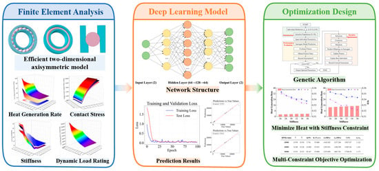
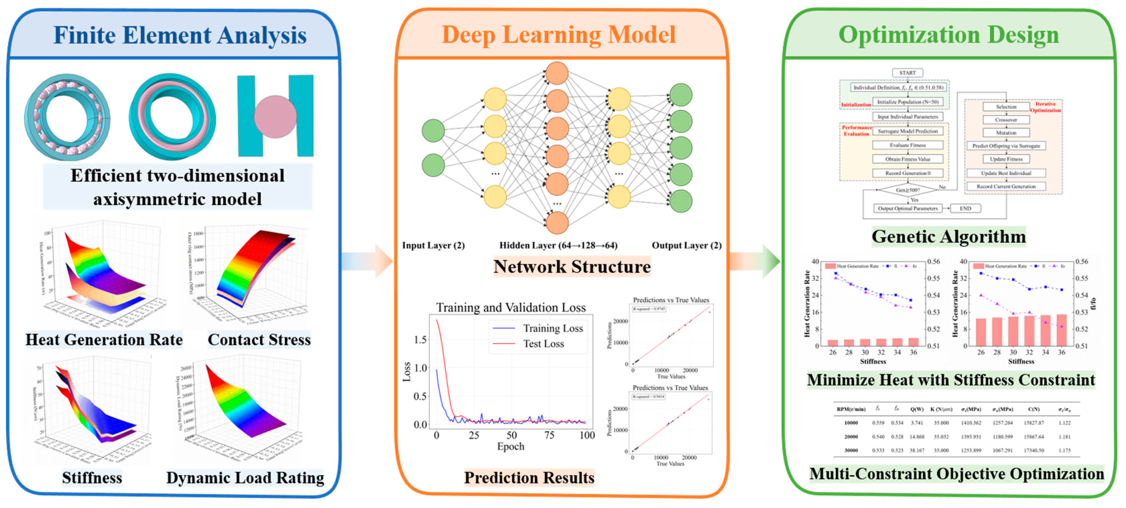
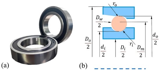
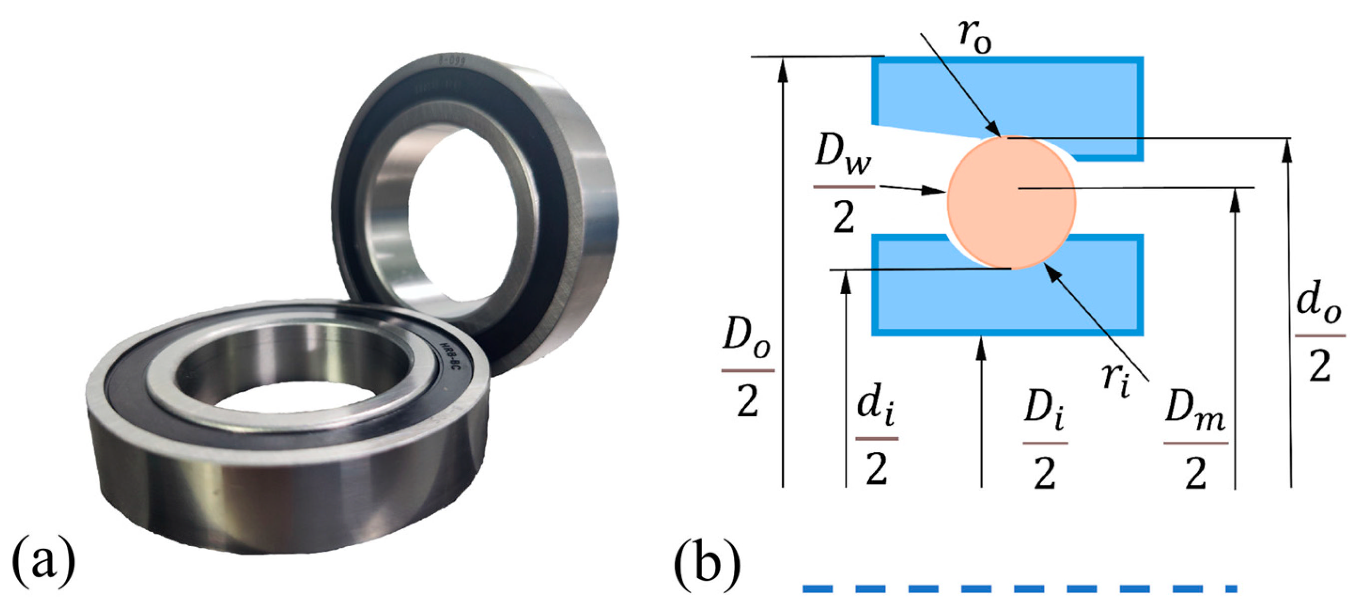
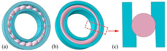
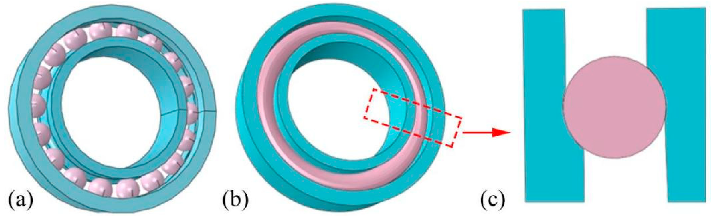
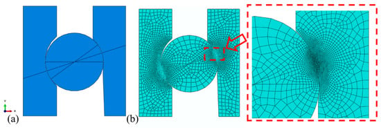
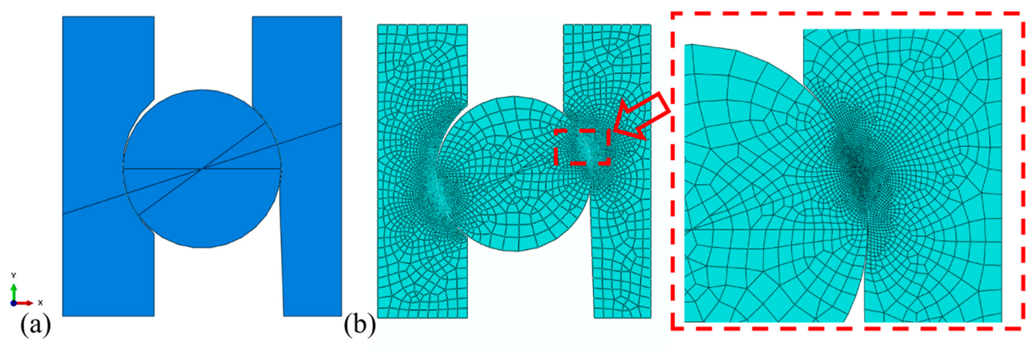
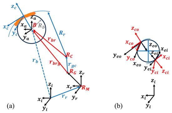
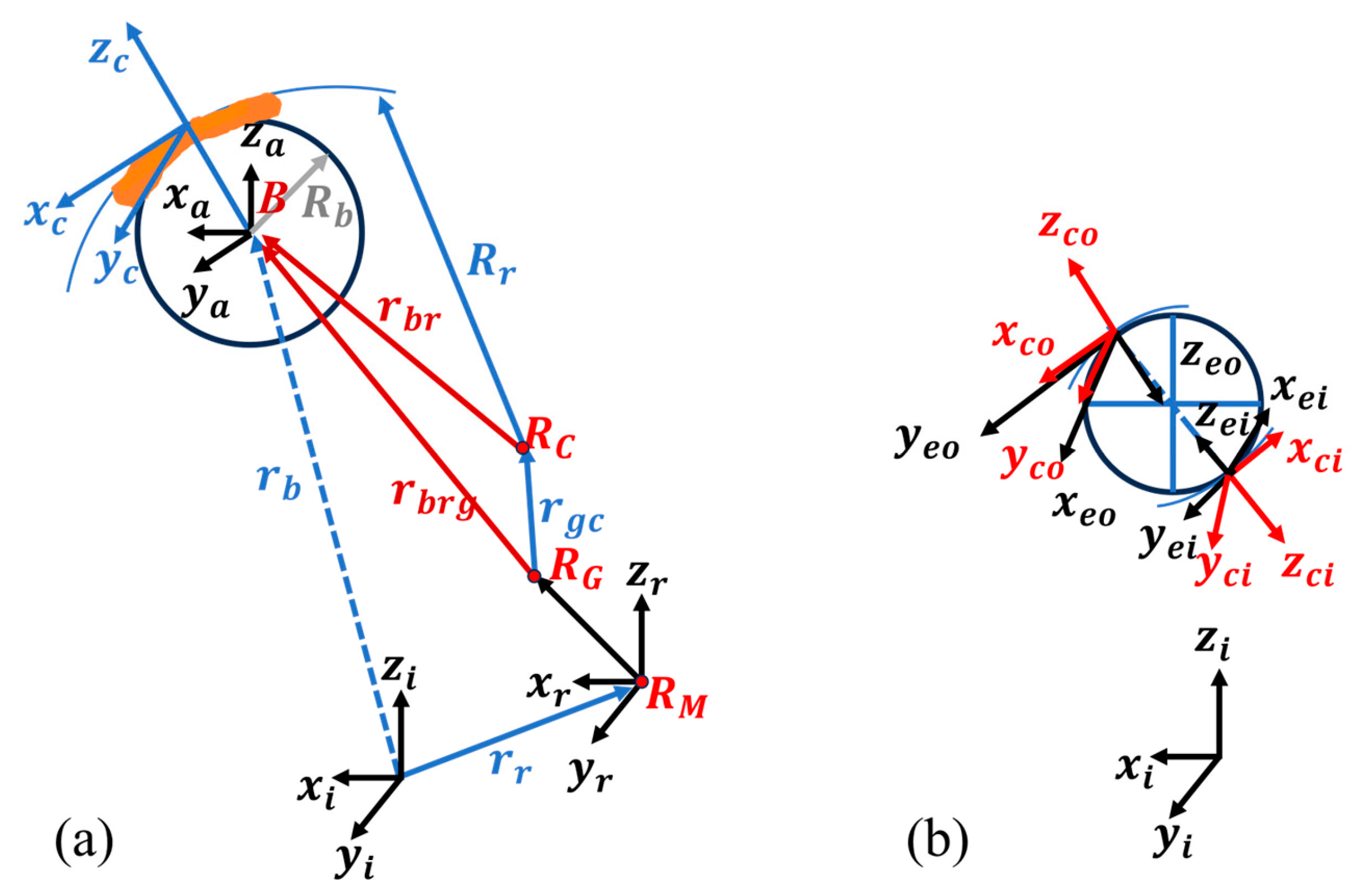
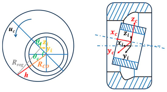
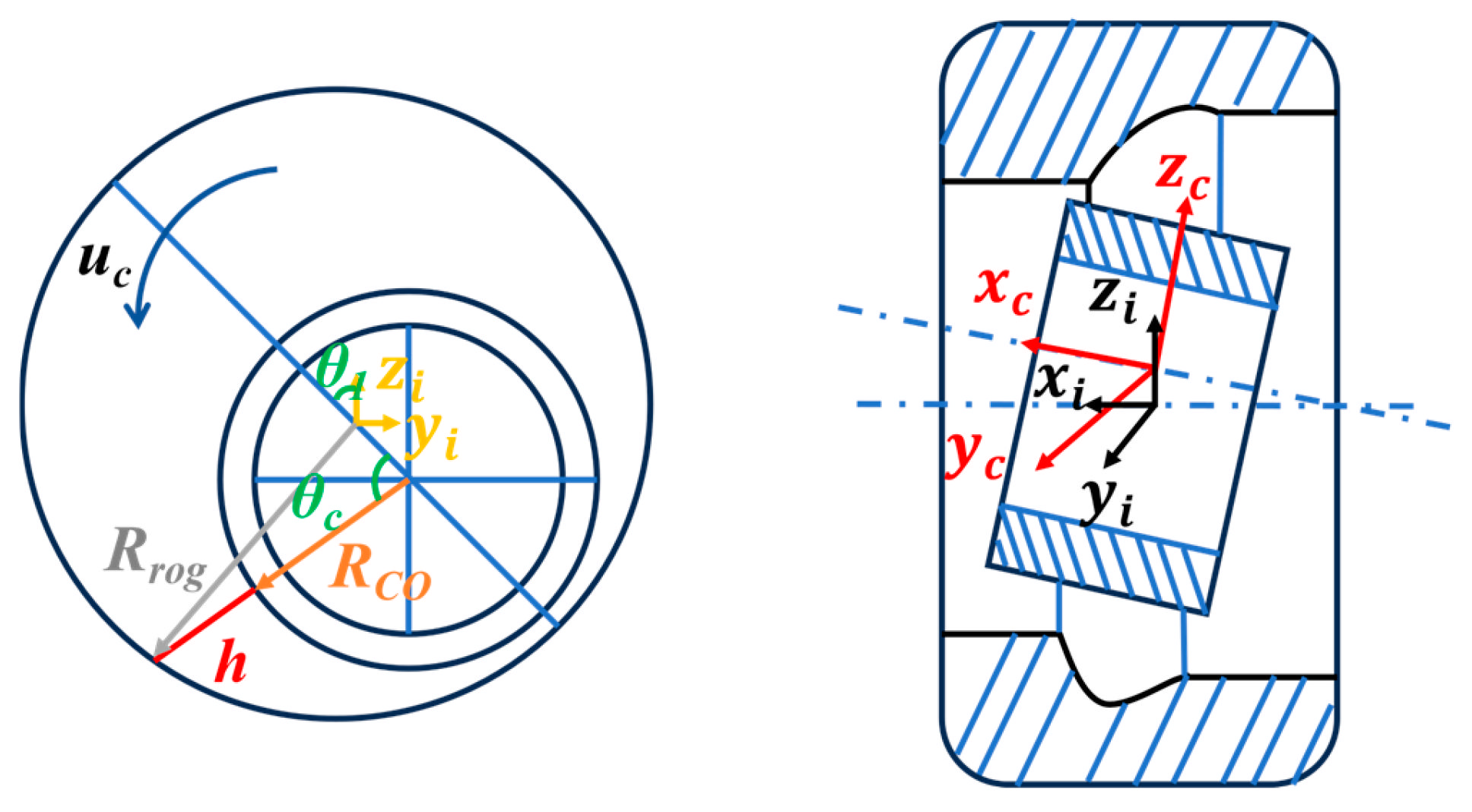
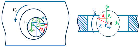
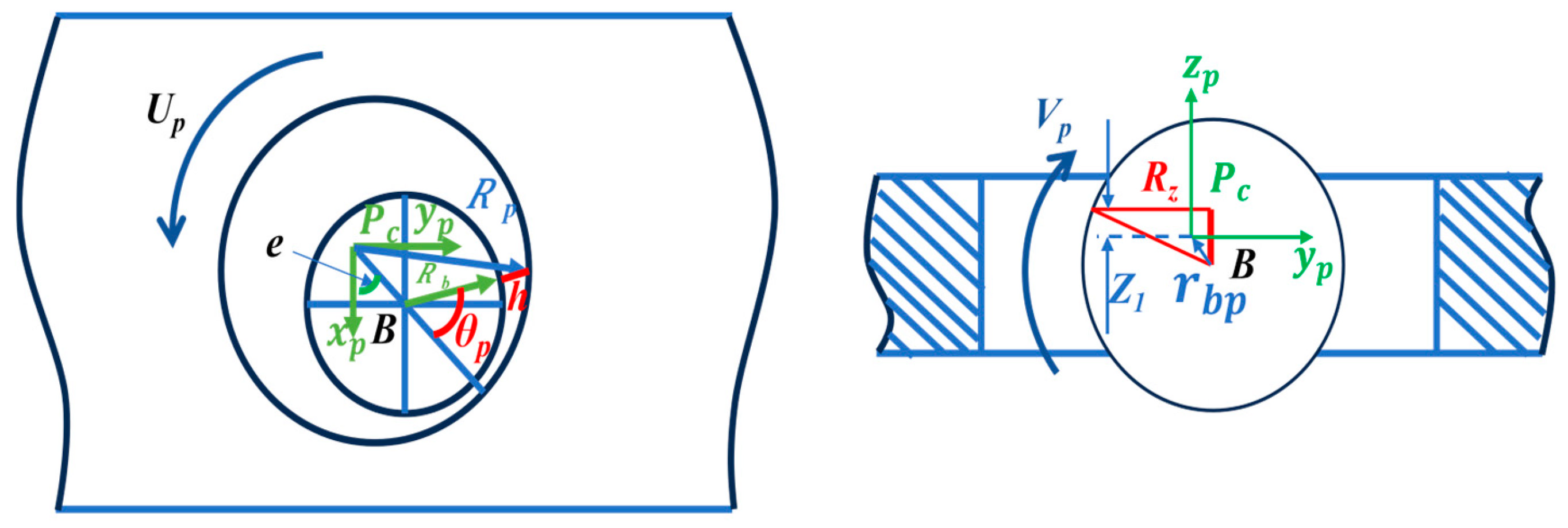
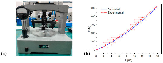
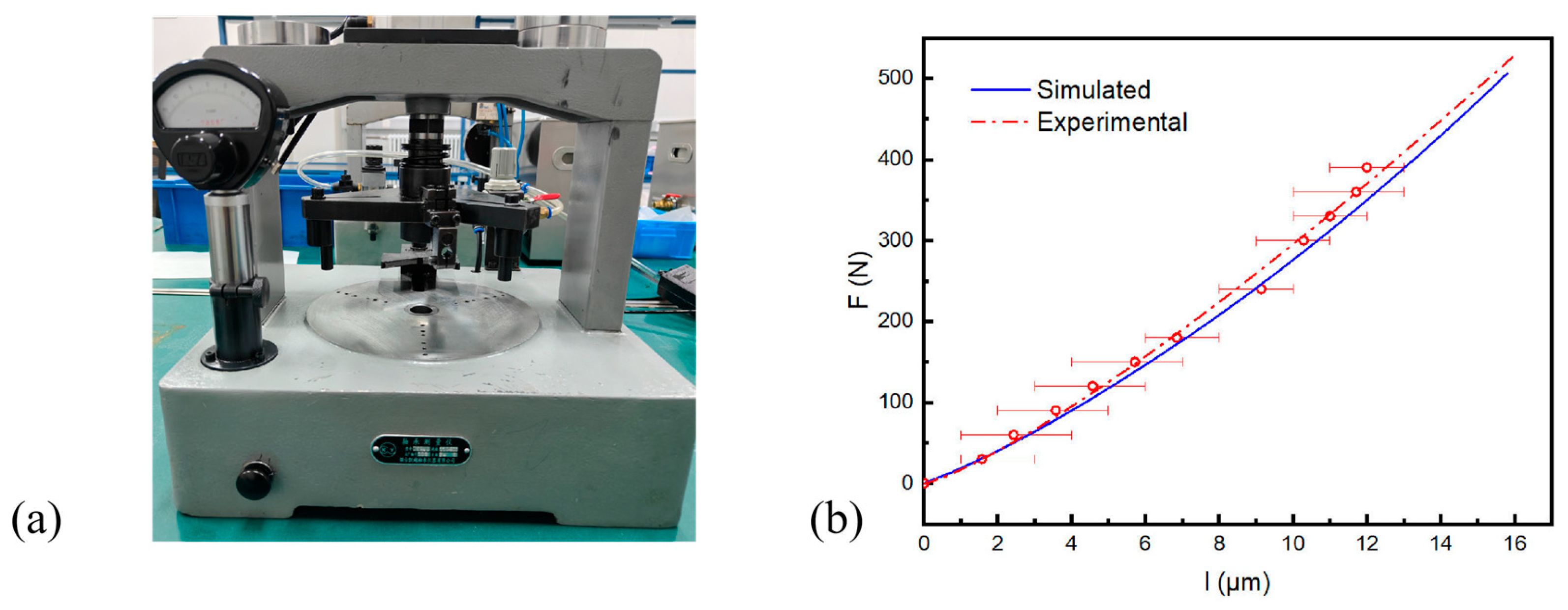
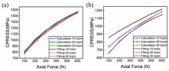
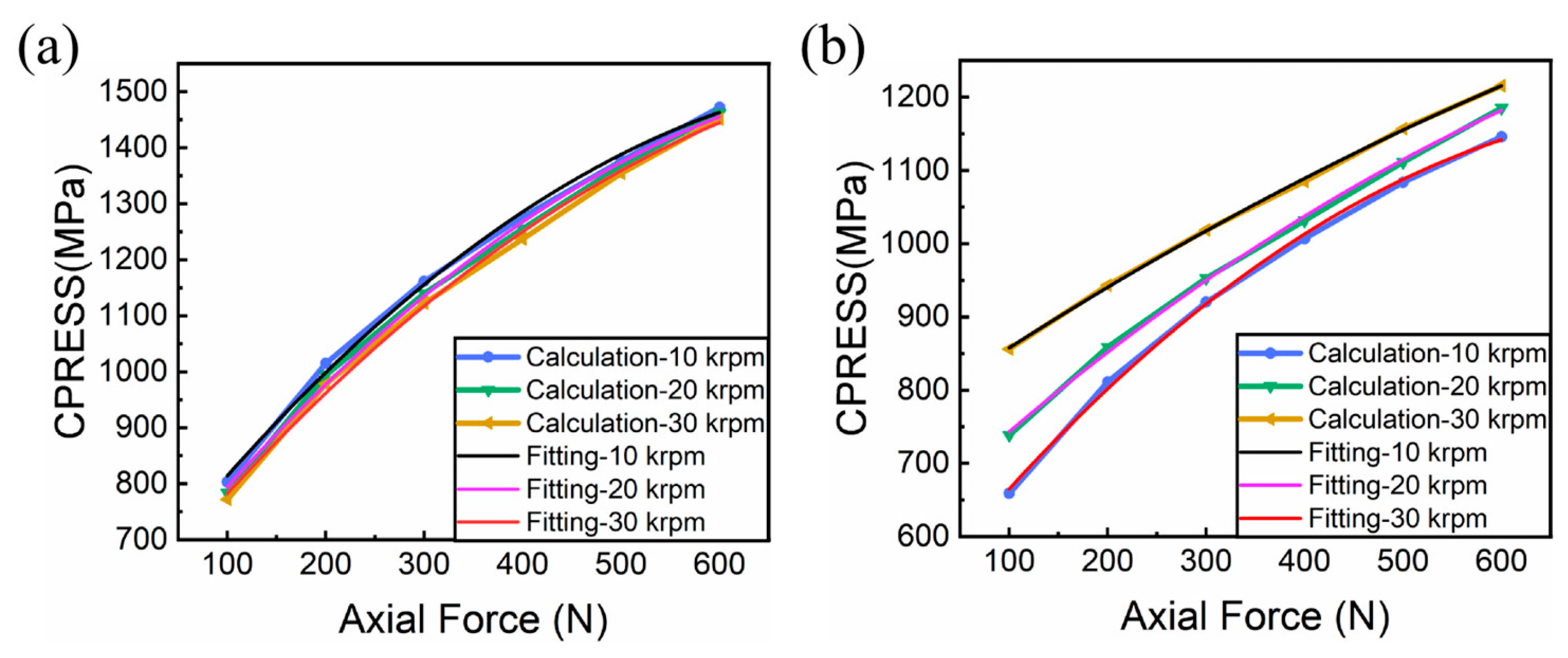
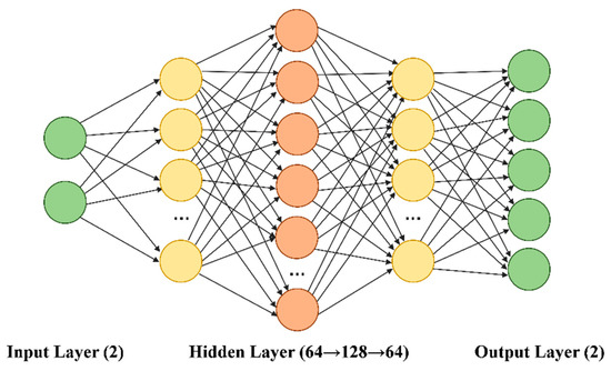
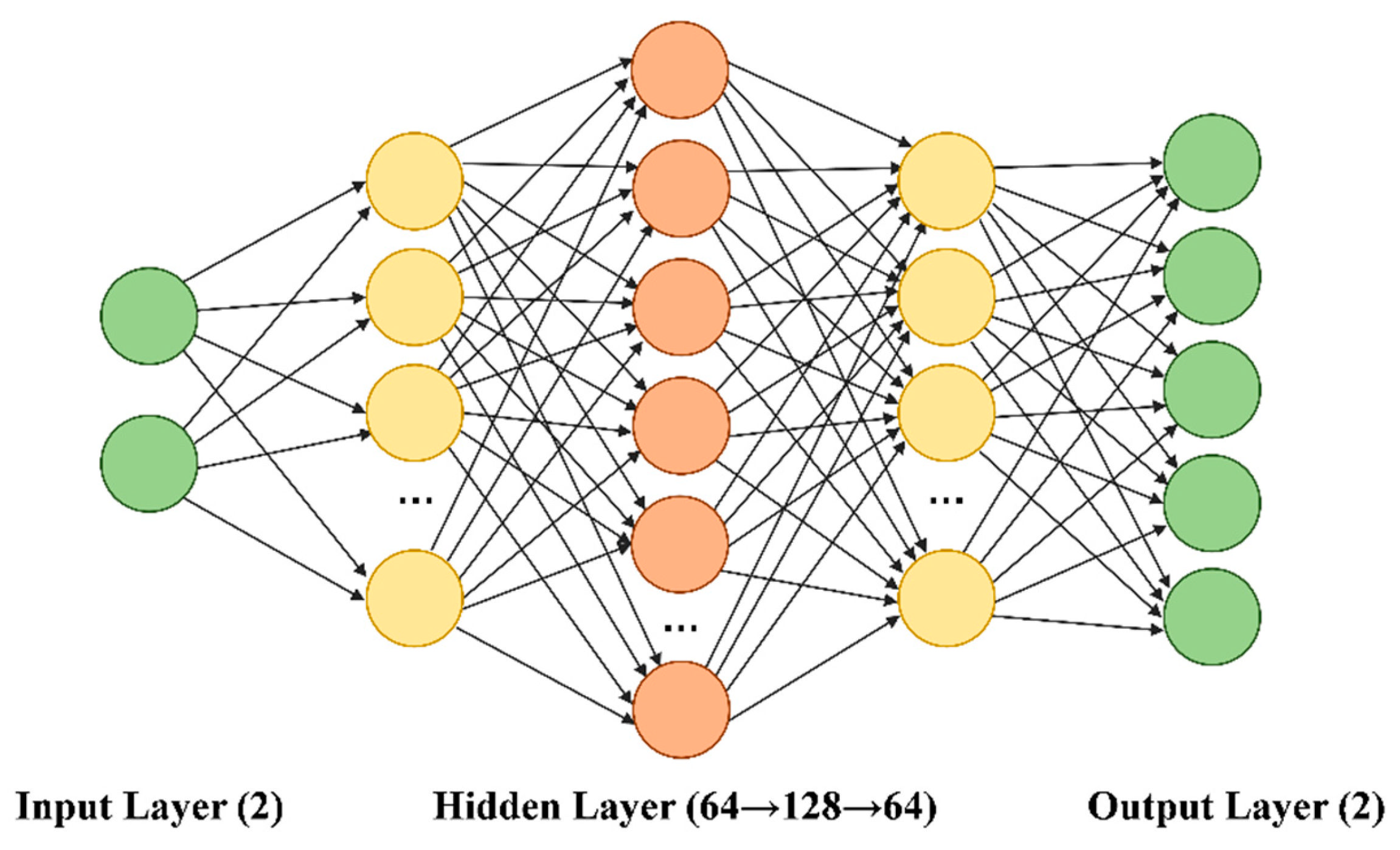
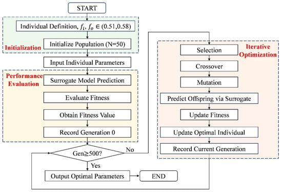
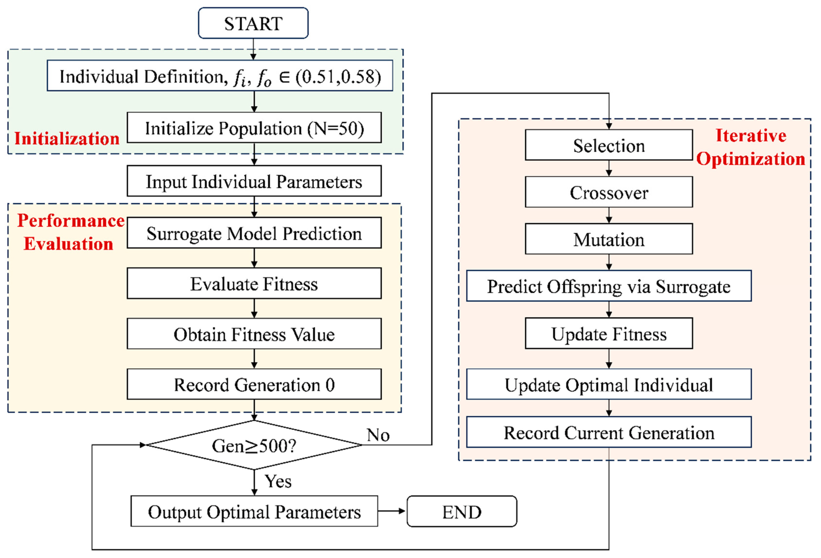
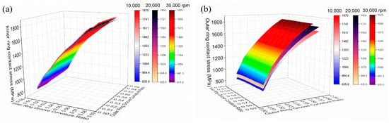
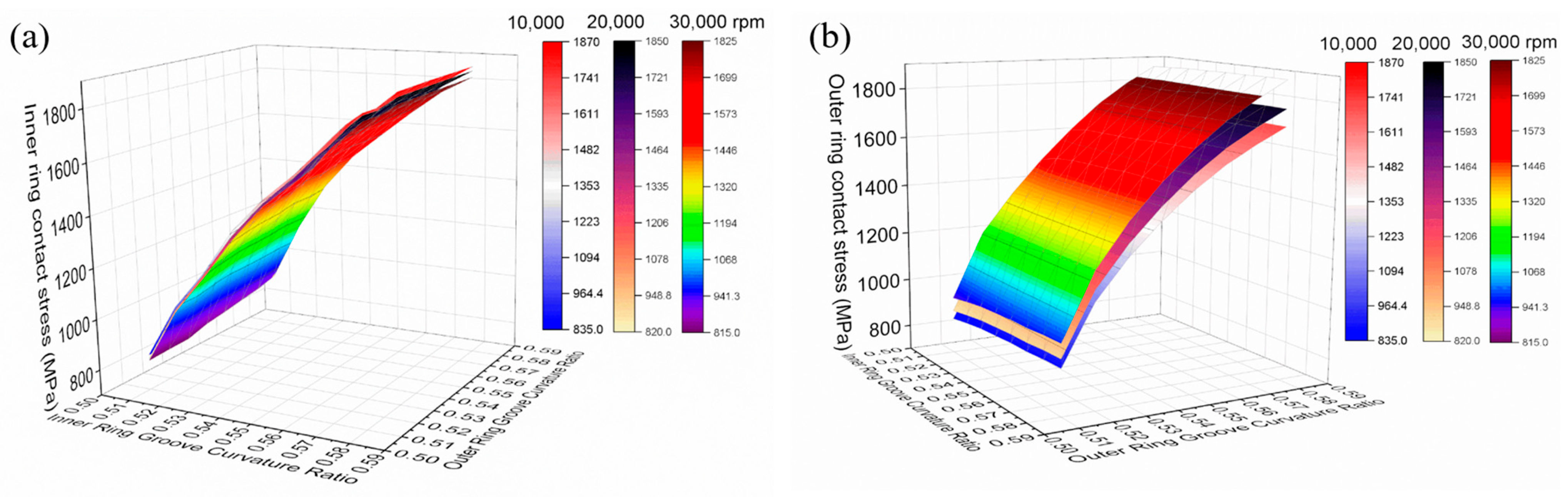
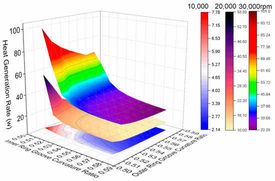
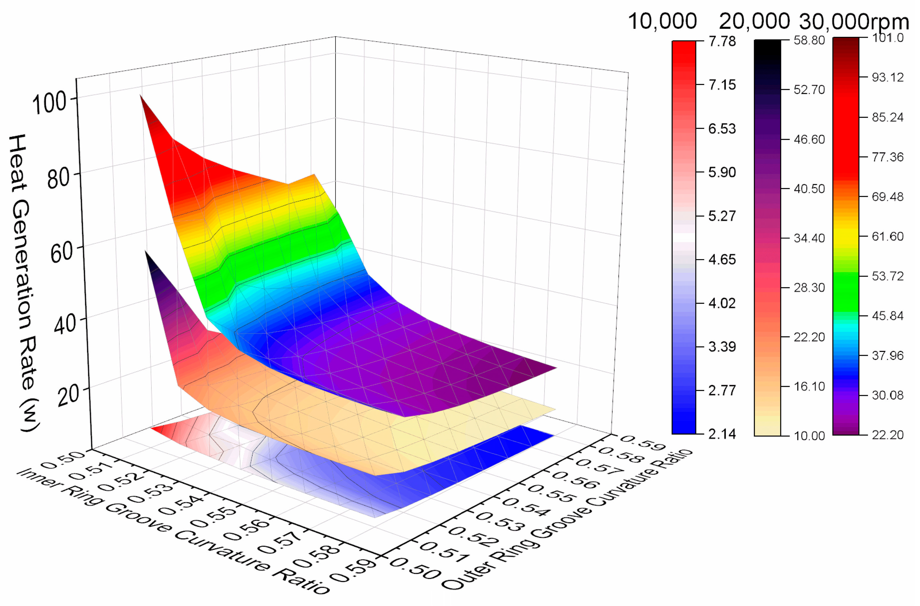
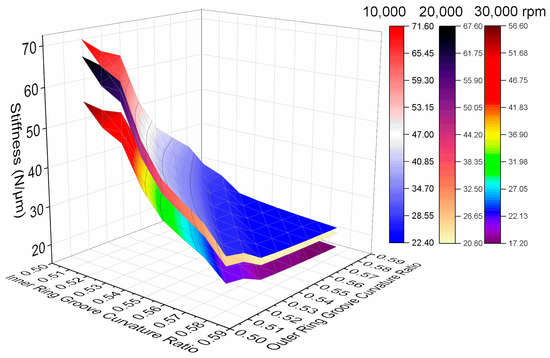
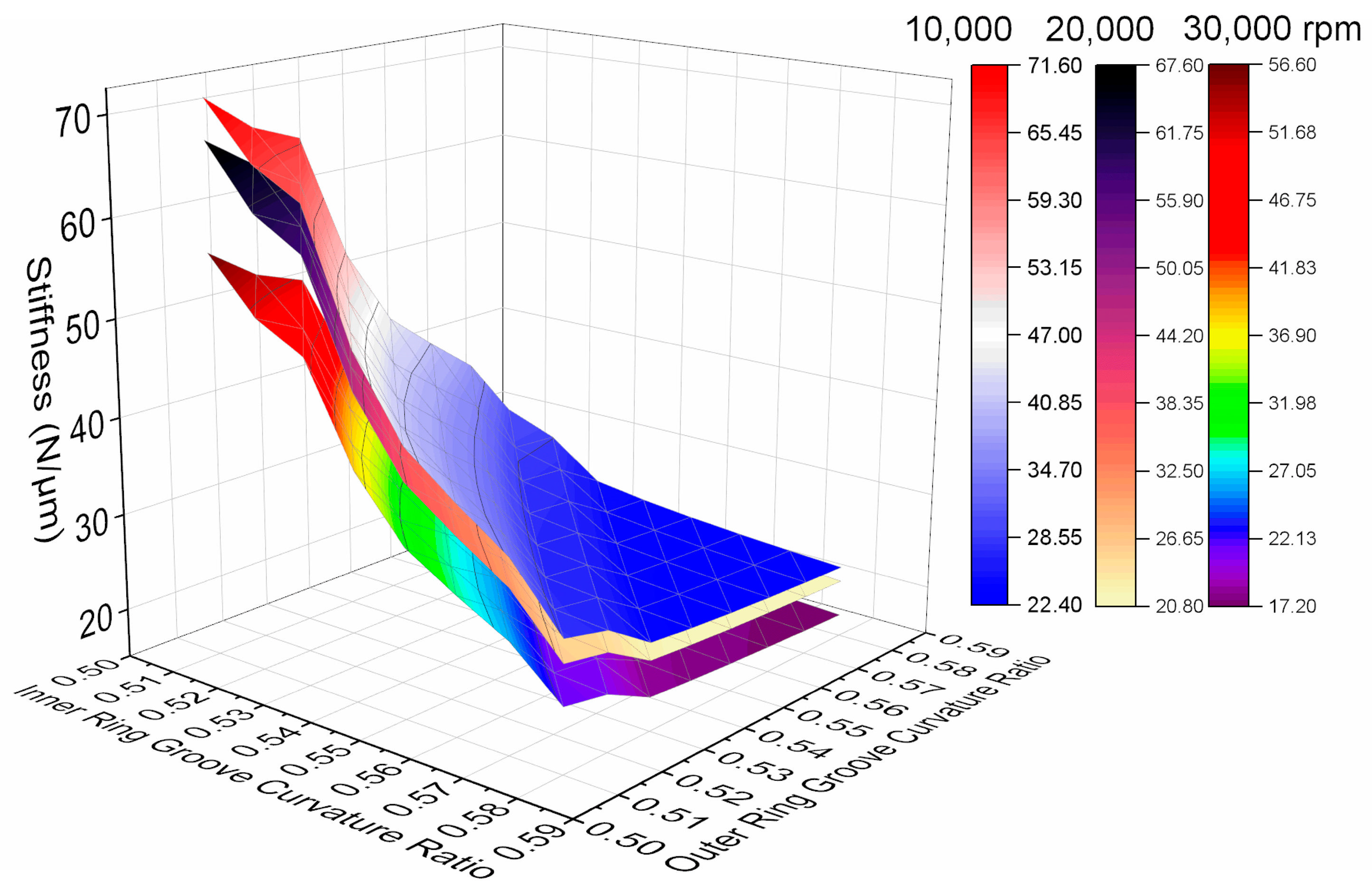
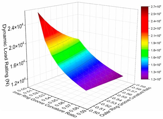
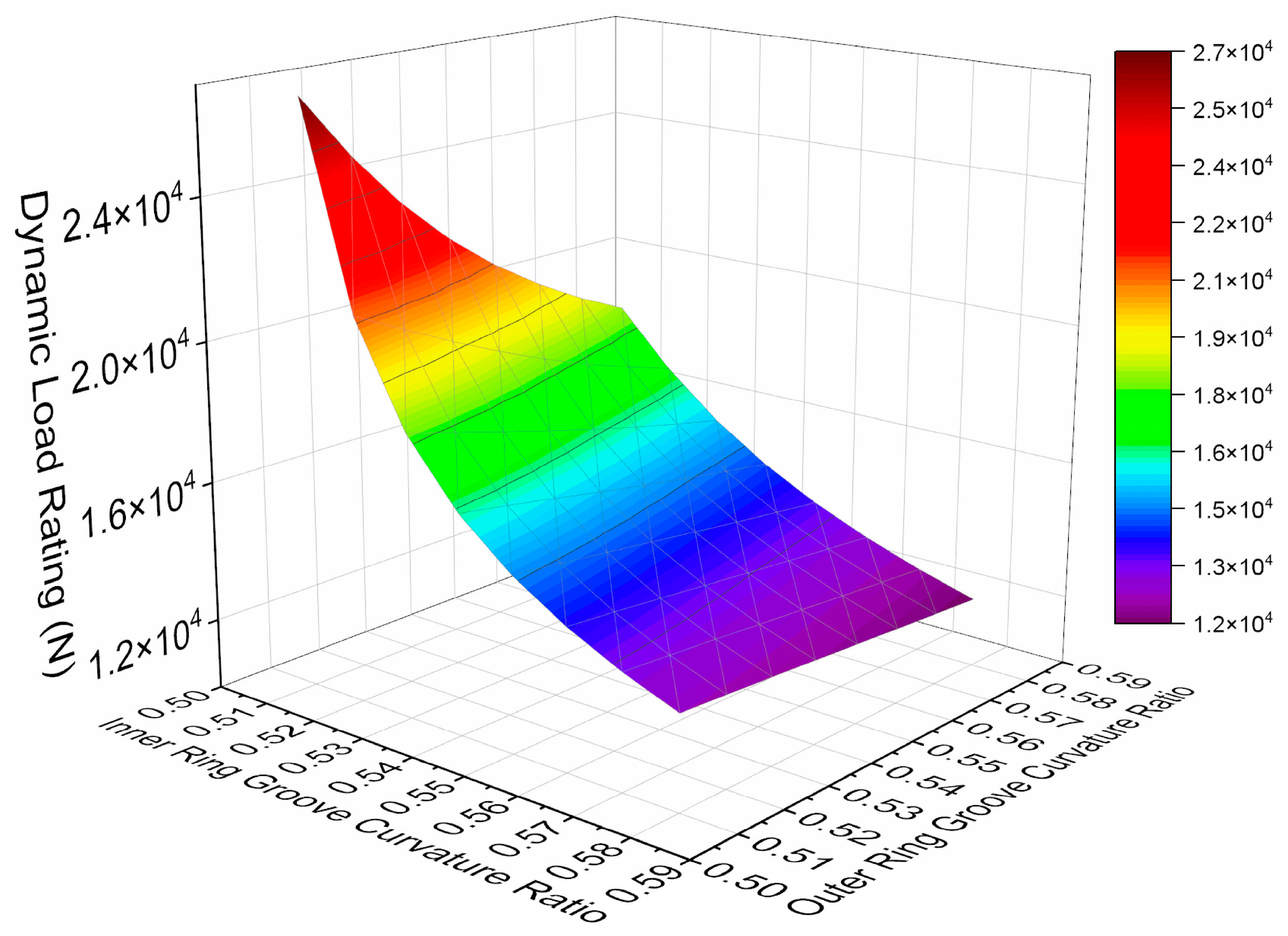
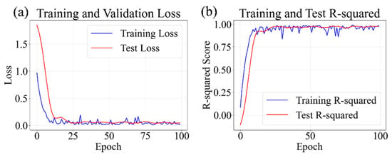
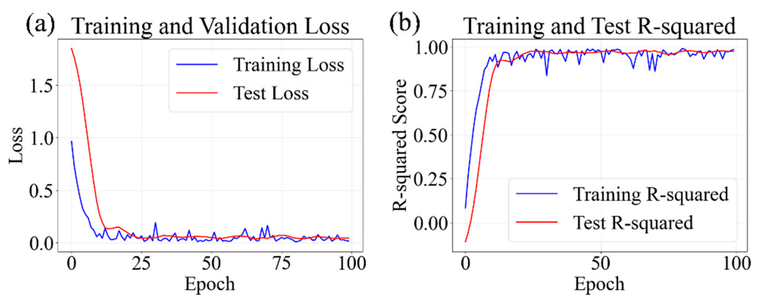
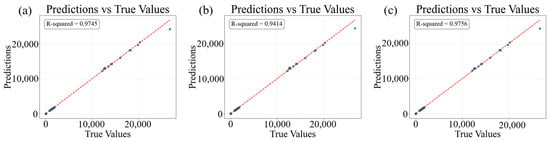
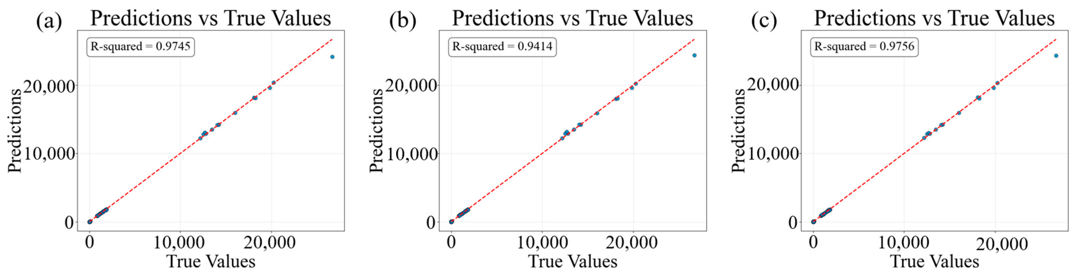
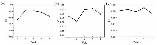
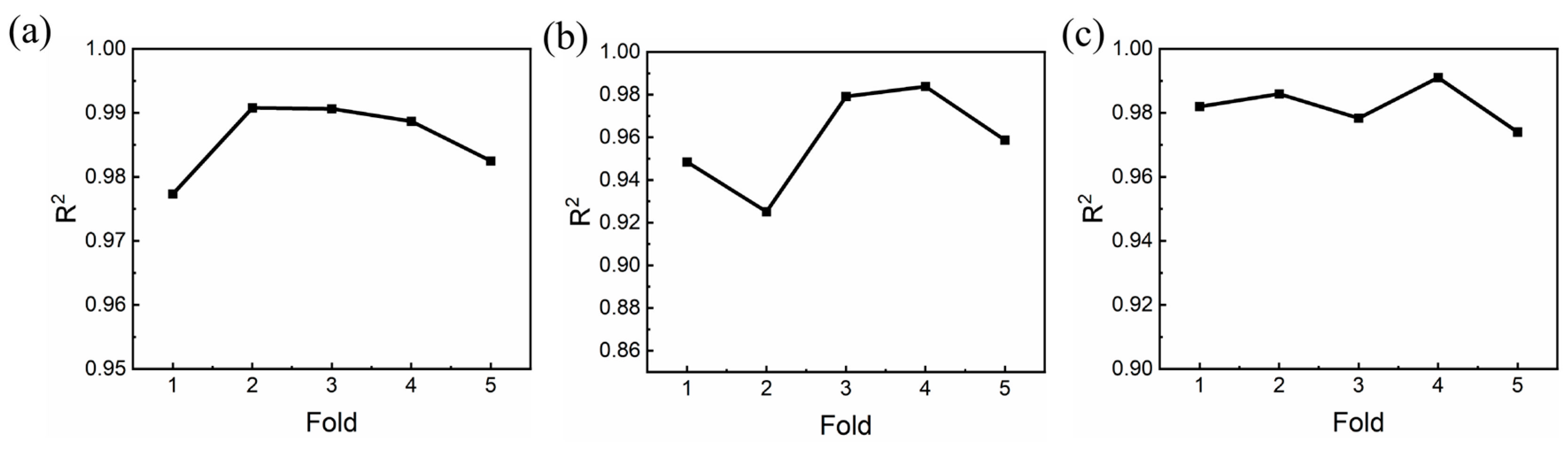
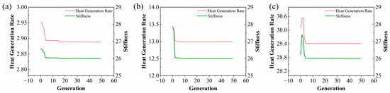
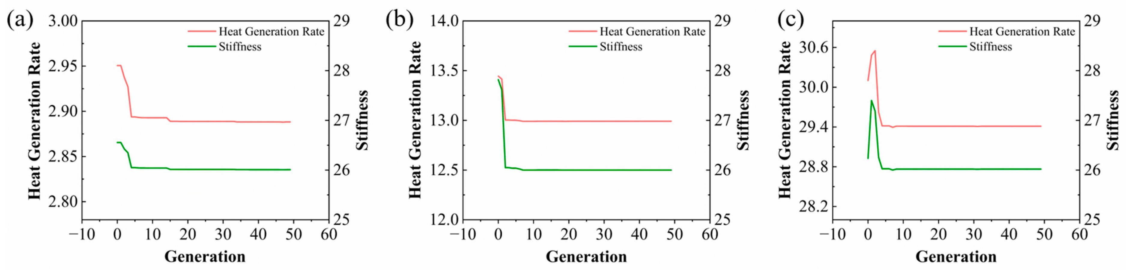
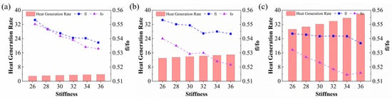
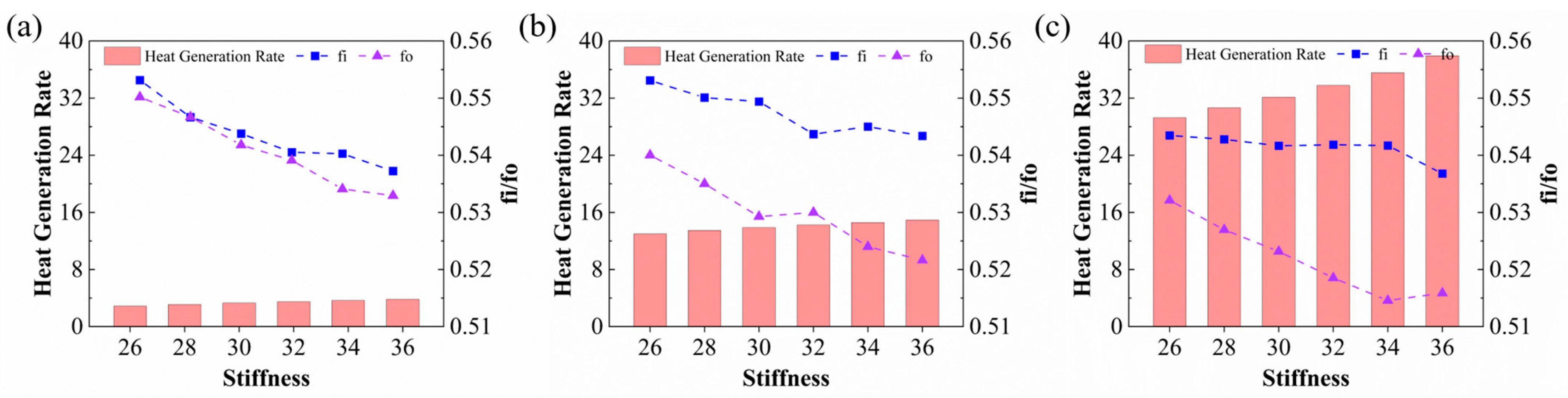

Disclaimer/Publisher’s Note: The statements, opinions and data contained in all publications are solely those of the individual author(s) and contributor(s) and not of MDPI and/or the editor(s). MDPI and/or the editor(s) disclaim responsibility for any injury to people or property resulting from any ideas, methods, instructions or products referred to in the content. |
© 2026 by the authors. Licensee MDPI, Basel, Switzerland. This article is an open access article distributed under the terms and conditions of the Creative Commons Attribution (CC BY) license.