Deep Gamma Damage Process for Offline Posterior Damage-Coordinate Assessment of Rolling Bearing Degradation

Abstract

This study proposes a deep Gamma damage process (DGDP) with rolling Bayesian updating for offline posterior damage-coordinate assessment of rolling bearing degradation. Time-domain, frequency-domain, and time-frequency features are extracted from complete run-to-failure vibration records in the XJTU-SY and PHM2012 bearing datasets. After smoothing, normalization, degradation-direction alignment, and fixed feature screening, nine degradation-sensitive features are retained and a principal-component-analysis-based health indicator (PCA-HI) is constructed. The PCA-HI is then converted into a monotone non-decreasing normalized cumulative damage trajectory, by which the life evolution of each bearing is represented in a posterior damage coordinate from $D=0$ to $D=1$. A deep sequence model parameterizes the Gamma distribution of the next damage increment, rolling Bayesian rate updating incorporates observed increments in the offline reconstructed damage prefix, and Monte Carlo threshold crossing assesses the crossing-time distribution on this posterior damage scale. To characterize the applicability boundary and the behavior of the proposed framework under controlled replay, fixed-ratio truncation at 20%, 40%, 60%, and 80%, fixed-initial-window replay, method comparison, and ablation experiments are conducted. The method is intended for offline posterior damage-coordinate assessment and should not be interpreted as calibrated prefix-only online RUL prediction.

1. Introduction

Rolling bearings are among the most widely used and failure-critical components in rotating machinery. Bearing faults may lead to machine shutdowns, production interruptions, and safety risks; therefore, degradation modeling from vibration measurements is a central task in machinery condition monitoring, fault diagnosis, and prognostics and health management [1,2,3,4,5]. For public accelerated run-to-failure datasets, complete vibration records can be used not only for model fitting but also for offline full-life degradation trajectory analysis, characterization of pre-failure damage accumulation, and posterior damage-coordinate assessment. Compared with a single final crossing-time estimate, a probabilistic assessment provides median crossing times, interval estimates, and coverage rates, thereby describing uncertainty and risk boundaries during degradation.

Deep learning and transfer learning have been extensively investigated for bearing remaining useful life (RUL) estimation [6,7,8,9,10,11,12,13,14,15,16,17]. These methods can learn nonlinear mappings from vibration signals or degradation features and can reduce distribution discrepancies between source and target conditions in cross-condition scenarios. However, many existing approaches are still formulated as deterministic RUL regression, and the model output is often a single life value. For full-life bearing data with evident stochastic degradation characteristics, deterministic regression alone weakens the representation of prediction intervals, failure probabilities, and local rapid-degradation risks. In addition, long healthy-stage records and short pre-failure transitions can cause models to fit the stationary portion excessively while responding insufficiently to critical damage-increment changes near failure.

Stochastic-process models provide a natural framework for probabilistic degradation assessment. Model-driven degradation approaches provide interpretable representations of degradation mechanisms and stochastic evolution, although their applicability depends on the assumed degradation law and available physical information [18]. A Gamma process is well suited for non-negative and monotone cumulative degradation [19]; a Wiener process describes continuous degradation trajectories with stochastic perturbations and is frequently used for degradation data analysis and RUL distribution estimation [20,21,22]; Bayesian updating incorporates local observations from a test bearing into the model prior. Conventional stochastic-process methods are interpretable, but they often depend on restrictive parametric assumptions and are therefore limited in exploiting high-dimensional degradation features and complex cross-condition patterns. Deep neural networks provide nonlinear representation capability [23,24,25,26,27,28,29]; however, a direct output of life distributions may lack a monotone damage constraint consistent with the physical degradation process. The present study combines these two ideas by first mapping full-life bearing trajectories to a monotone posterior damage coordinate, then learning damage-increment distributions with a deep sequence network, and finally assessing threshold-crossing times through a Gamma process.

On this basis, a deep Gamma damage process (DGDP) framework is proposed for offline full-life degradation trajectories. The framework uses degradation information represented by PCA-HI and maps different bearings to a unified posterior damage coordinate through monotone non-decreasing cumulative damage construction. A deep sequence network is then used to parameterize the Gamma distribution of the next damage increment. Rolling Bayesian rate updating, posterior fast-state usage, and Monte Carlo threshold-crossing simulation are combined to assess the crossing-time distribution on this damage coordinate. This DGDP framework is intended for offline posterior damage-coordinate assessment of complete run-to-failure records and should not be interpreted as calibrated prefix-only RUL prediction.

The main novelty lies in integrating an offline posterior damage coordinate, deep Gamma increment parameterization, rolling Bayesian updating, and probabilistic threshold-crossing assessment within a unified framework. The main contributions are summarized as follows:

• An offline full-life degradation modeling procedure is constructed from nine degradation features and PCA-HI to monotone non-decreasing cumulative damage, transforming degradation assessment into damage-increment distribution modeling and posterior threshold-crossing analysis.
• A conditional Gamma damage-increment model parameterized by a deep sequence network is designed. Transformer-GRU is retained as the pre-specified default parameterizer, while Transformer-only and GRU-only backbones are compared to avoid attributing the final performance to a single network structure.
• Rolling Bayesian rate updating and posterior fast-state usage are incorporated into the replay protocol. Recent observed increments in the posterior damage prefix correct the deep-model prior, while the fast score is treated as a posterior explanatory feature rather than a prefix-available deployment signal.
• Fixed-ratio truncation is used as the primary applicability-boundary experiment, while fixed-initial-window replay and method comparison are reported as controlled offline posterior replay demonstrations. Mean absolute error (MAE), root mean squared error (RMSE), 90% prediction interval coverage probability (PICP90), 90% mean prediction interval width (MPIW90), normalized MPIW90 (nMPIW90), and continuous ranked probability score (CRPS) are reported with explicit statistical units and applicability boundaries.

The remainder of this paper is organized as follows. Section 2 presents the overall workflow, datasets, feature processing, PCA-HI construction, monotone cumulative damage construction, and the deep Gamma damage process model. Section 3 reports the experimental settings and results. Section 4 discusses the method characteristics, applicability boundaries, and limitations. Section 5 concludes the paper.

2. Materials and Methods

2.1. Overall Workflow

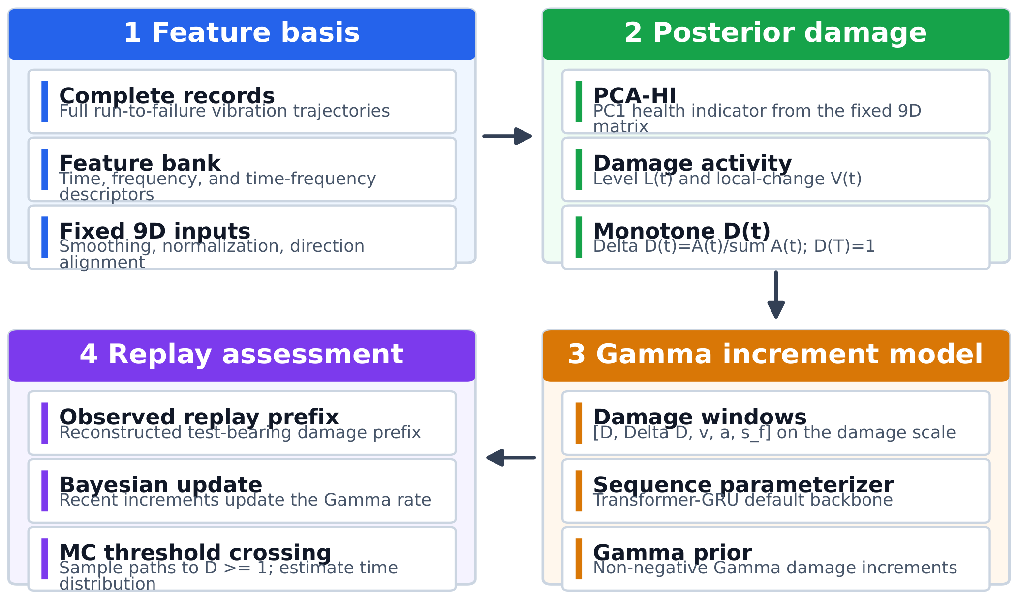
The overall workflow of the proposed method is shown in Figure 1. First, multi-domain degradation features are extracted from complete-life raw vibration signals and reduced to nine fixed screened features. Second, PCA-HI is constructed and transformed into a monotone posterior cumulative damage coordinate. Third, windows of the cumulative damage process are used to train a deep Gamma increment model. Finally, rolling Bayesian updating and Monte Carlo threshold-crossing analysis are performed on the offline reconstructed damage trajectory of the test bearing. Because normalization, PCA-HI, and damage construction all use complete life trajectories, the reported results represent probabilistic assessment in an offline posterior damage coordinate rather than prefix-only early-stage prognostic assessment.

2.2. Datasets and Raw Signal Processing

Two public accelerated run-to-failure bearing datasets, XJTU-SY and PHM2012/PRONOSTIA, are used in this study [30,31]. The XJTU-SY dataset was released by Xi’an Jiaotong University (Xi’an, China), and the PHM2012/PRONOSTIA platform was developed by FEMTO-ST Institute (Besancon, France). The public dataset descriptions report LDK UER204 insert ball bearings in the XJTU-SY dataset and NSK 6804DD deep-groove ball bearings in the PHM2012 dataset. The XJTU-SY dataset includes three combinations of rotational speed and radial load. For each sampling file, horizontal and vertical vibration signals were collected at 25.6 kHz for 1.28 s with a sampling interval of 1 min. The PHM2012 dataset was obtained from the PRONOSTIA platform under multiple operating conditions. Each sampling file contains a 0.1 s vibration record acquired at 25.6 kHz with a sampling interval of 10 s. In both datasets, vibration sensors recorded complete bearing life sequences from healthy states to failure, making the datasets suitable for offline degradation trajectory reconstruction and posterior damage-coordinate assessment. The main operating conditions and sampling settings are listed in

Table 1. Operating conditions, bearing models, and sampling settings of the datasets.

Dataset	Condition	Bearing Model	Speed	Radial Load	Sampling Setting
XJTU-SY	C1	LDK UER204	2100 r/min	12 kN	25.6 kHz, 1.28 s/1 min horizontal/vertical channels
	C2		2250 r/min	11 kN	25.6 kHz, 1.28 s/1 min horizontal/vertical channels
	C3		2400 r/min	10 kN	25.6 kHz, 1.28 s/1 min horizontal/vertical channels
PHM2012	C1	NSK 6804DD	1800 r/min	4000 N	25.6 kHz, 0.1 s/10 s horizontal/vertical channels
	C2		1650 r/min	4200 N	25.6 kHz, 0.1 s/10 s horizontal/vertical channels
	C3		1500 r/min	5000 N	25.6 kHz, 0.1 s/10 s horizontal/vertical channels

.

Detailed lubrication parameters, including lubricant type, grease quantity, relubrication condition, and contamination level, were unavailable in the original dataset references consulted in this study. Therefore, the influence of lubrication could not be evaluated separately in the present analysis.

A fixed holdout split is adopted, and the test bearings are not used to construct training windows. The detailed split is shown in

Table 2. Bearing split and model-selection protocol.

Dataset	Conditions	Training Bearings	Test Bearings	Validation/Selection
XJTU-SY	C1–C3	C1: Bearing1_2, Bearing1_4, Bearing1_5 C2: Bearing2_1, Bearing2_3, Bearing2_4, Bearing2_5 C3: Bearing3_1, Bearing3_2, Bearing3_3, Bearing3_4	C1: Bearing1_1, Bearing1_3 C2: Bearing2_2 C3: Bearing3_5	No independent validation bearing; holdout windows from training bearings select best epoch
PHM2012	C1–C3	C1: Bearing1_1, Bearing1_3, Bearing1_4, Bearing1_5, Bearing1_6, Bearing1_7 C2: Bearing2_3, Bearing2_5, Bearing2_6, Bearing2_7 C3: Bearing3_1, Bearing3_2	C1: Bearing1_2 C2: Bearing2_1, Bearing2_2, Bearing2_4	No independent validation bearing; holdout windows from training bearings select best epoch

. The holdout windows used for best-epoch selection were sampled only from the training bearings, and no windows from the test bearings were used for gradient updating or model selection. During training, the best epoch was selected according to the next-step damage-increment metric on the holdout windows, whereas the hyperparameters followed a fixed configuration. This setting prevents test bearings from participating in gradient updating or model selection. However, no independent validation bearing is specified; therefore, the protocol is not equivalent to a strict three-way train/validation/test split. Independent validation bearings or nested cross-validation would further reduce methodological bias associated with model selection.

For each bearing, the full-life vibration sequence is first formed according to the chronological order of sampling files. Time-domain, frequency-domain, and time-frequency features are then extracted from each sampling segment. The horizontal channel is used for XJTU-SY, and each raw signal file is downsampled to 2048 points. The horizontal channel is also used for PHM2012, where each acc file contains 2560 sampling points. This single-channel setting follows a predefined feature-processing scheme and reduces the modeling complexity of the unified dual-dataset analysis; vertical-channel and dual-channel fusion comparisons are not included as experimental conclusions. To reduce the influence of random noise, the feature sequences are processed by Savitzky–Golay smoothing [32], Min–Max normalization, and degradation-direction alignment. Because this study focuses on offline full-life degradation analysis, normalization and PCA-HI construction use complete bearing trajectories and do not define a prefix-only early-stage assessment protocol.

2.3. Thirty-Six Base Features and Nine Fixed Screened Features

For each sampling segment, 36 base degradation features are extracted, including 16 time-domain features, 12 frequency-domain features, and 8 time-frequency features. Let the sampling segment be $x=\{x_1,x_2,\dots ,x_N\}$. Representative time-domain features include root mean square, peak-to-peak value, skewness, kurtosis, waveform factor, crest factor, impulse factor, and margin factor. For example, root mean square and kurtosis are expressed as

$$x_{\mathrm{rms}}=\sqrt{{\displaystyle \frac{1}{N}}\sum _{i=1}^N{x}_i^2},$$

(1)

$$K={\displaystyle \frac{1}{N}}{\displaystyle \sum _{i=1}^N}{\left({\displaystyle \frac{x_i-\overline{x}}{\sigma }}\right)}^4,$$

(2)

where $\overline{x}$ and $\sigma$ are the signal mean and standard deviation, respectively. As local bearing damage develops, impact amplitudes and higher-order statistics generally change markedly.

Frequency-domain features are calculated after obtaining the amplitude spectrum $s_k$ and the corresponding frequency $f_k$ through the fast Fourier transform. They mainly describe spectral energy distribution, frequency centroid, and spectral-shape variation. The frequency centroid is defined as

$$f_c={\displaystyle \frac{{\sum }_{k=1}^M{f}_k{s}_k}{{\sum }_{k=1}^M{s}_k}},$$

(3)

where M is the number of spectral points. Time-frequency features are obtained through three-level wavelet packet decomposition, resulting in eight terminal-band energies:

$$E_j={\displaystyle \sum _{n=1}^{L_j}}{c}_{j,n}^2,j=1,2,\dots ,8,$$

(4)

where $c_{j,n}$ is the wavelet-packet coefficient of the jth frequency band.

Feature normalization uses the column-wise Min–Max form:

$$z_{i,j}=\left\{\begin{array}{cc}{\displaystyle \frac{x_{i,j}-x_j^{min}}{x_j^{max}-x_j^{min}}},\hfill & x_j^{max}>x_j^{min},\hfill \\ 0,\hfill & x_j^{max}=x_j^{min}.\hfill \end{array}\right.$$

(5)

If a feature has a higher value at the early life stage than at the end of life, the direction is reversed by $1-z_{i,j}$ so that the feature generally increases with degradation.

Based on the 36 base features, a fixed feature-screening scheme is used to generate nine degradation features. For XJTU-SY, the candidate order is T6, T10, T12, T13, T16, F3, F10, F11, A0, and A1. After removing the sixth column, F3, the retained features are T6, T10, T12, T13, T16, F10, F11, A0, and A1. For PHM2012, a concatenated matrix is first formed from a fixed 10-dimensional candidate feature set, and the sixth column of the final concatenated matrix, T12/kurtosis, is then removed. The screening scheme follows an established feature-engineering procedure that mainly considers monotonicity, trendability, cross-bearing consistency, Spearman correlation with time or degradation labels, and an mRMR-style redundancy check [33]. It is kept unchanged in all experiments and is not reselected according to the test-bearing results. Thus, the fixed-initial-window replay demonstration, fixed-ratio truncation experiments, comparison experiments, and ablation experiments use the same feature entrance. Feature screening itself is not treated as a separate performance contribution. Appendix A summarizes the 36 base features, the fixed candidate set, the retained nine features, and the reason for removing the sixth candidate feature.

2.4. PCA-HI Construction

To compress multi-dimensional degradation features into an interpretable one-dimensional health indicator, principal component analysis is applied to the nine-dimensional normalized feature matrix $\mathbf{X}\in {\mathbb{R}}^{T\times 9}$ for each bearing, and the first principal component is used as the initial HI. This PCA-HI is a posterior health indicator reconstructed offline from the complete life trajectory. It is used to unify the damage coordinate and threshold-crossing assessment, and it does not represent a real-time health indicator that can be obtained solely from historical observations at a given prefix. Let the centered feature matrix be $\tilde{\mathbf{X}}$. The PCA projection is written as

$$\mathbf{h}=\tilde{\mathbf{X}}{\mathbf{w}}_1,$$

(6)

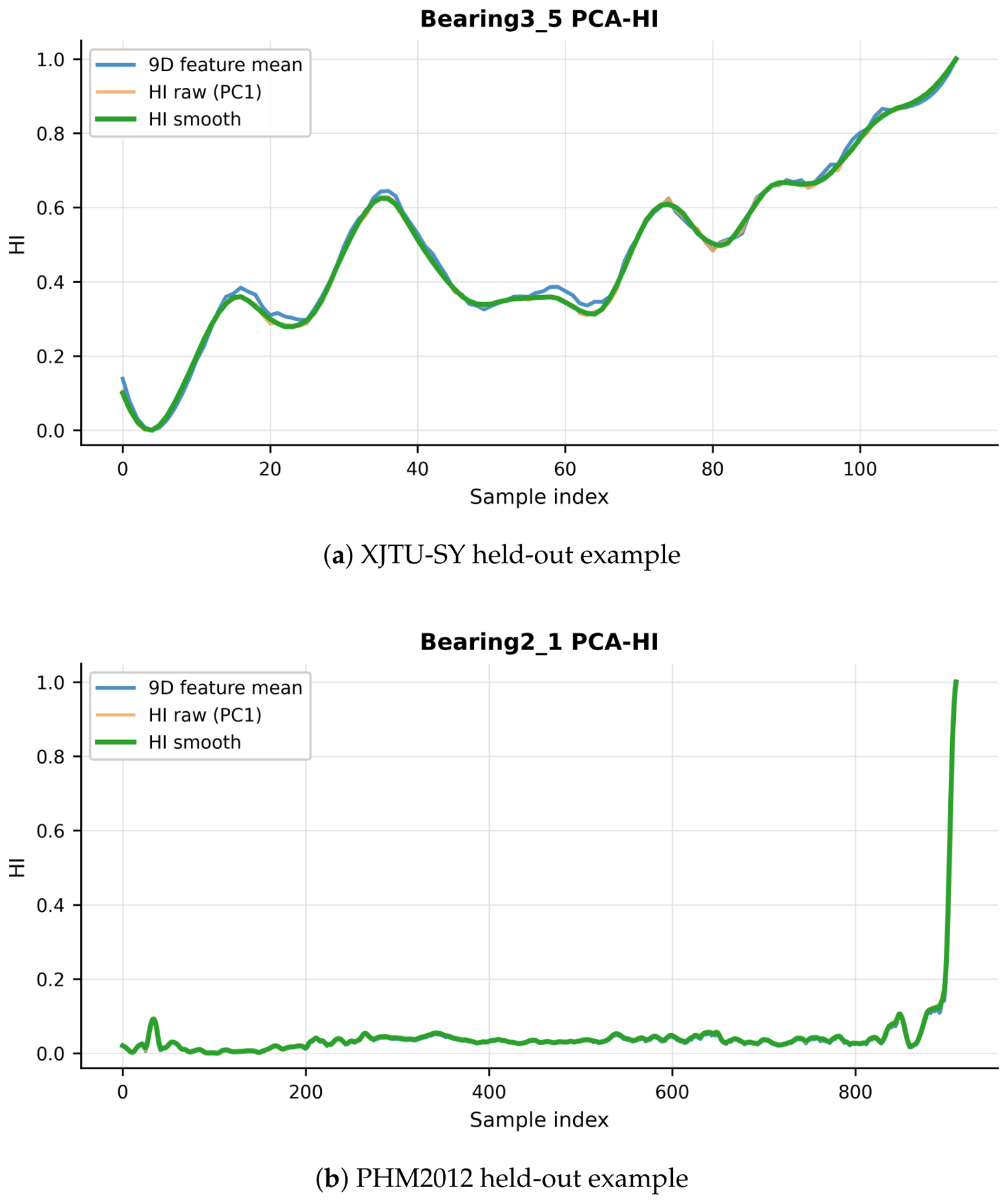
where ${\mathbf{w}}_1$ is the eigenvector corresponding to the maximum variance direction. The vector $\mathbf{h}$ is then normalized, direction-aligned, and smoothed to obtain $\mathrm{HI}\left(t\right)$. Figure 2 shows generated PCA-HI curves for representative post hoc examples under the offline reconstructed damage-coordinate protocol. These examples are provided to illustrate the offline reconstruction process. The results show that the XJTU-SY example exhibits clear multi-stage middle-to-late degradation, whereas evident degradation in the PHM2012 example is concentrated close to the end of life. This observation supports the use of a fast-degradation state in posterior replay, but does not imply that such a state is available in prefix-only deployment.

2.5. Monotone Cumulative Damage Construction

Because a Gamma process is commonly used for non-negative and monotone cumulative degradation [19], the PCA-HI is further converted into monotone non-decreasing cumulative damage. Since the object of this study is the offline full-life degradation trajectory, the normalization factors in the following equations are calculated from the complete life trajectory. The purpose is to map bearings with different lengths, operating conditions, and degradation rates to a unified posterior damage coordinate rather than to obtain a real-time damage scale available at a prefix. Accordingly, $D\left(t\right)$ denotes offline reconstructed normalized cumulative damage in this study. For each bearing, the smoothed HI is first trend-smoothed to obtain ${\mathrm{HI}}_{\mathrm{trend}}\left(t\right)$. The level term $L\left(t\right)$ and the local-change term $V\left(t\right)$ are then calculated and combined as the degradation activity:

$$A\left(t\right)=\sqrt{L{\left(t\right)}^2+V{\left(t\right)}^2}.$$

(7)

where $L\left(t\right)$ denotes the normalized degradation level and $V\left(t\right)$ denotes the local-change intensity. After non-negative transformation and smoothing of $A\left(t\right)$, the damage increment is obtained as

$$\Delta D\left(t\right)={\displaystyle \frac{A\left(t\right)}{{\sum }_{\tau =2}^{T}A\left(\tau \right)}},t=2,\dots ,T,$$

(8)

and cumulative damage is obtained by summation:

$$\begin{array}{cc}\hfill D\left(1\right)& =0,\hfill \\ \hfill D\left(t\right)& ={\displaystyle \sum _{\tau =2}^t}\Delta D\left(\tau \right),t=2,\dots ,T,\hfill \\ \hfill D\left(T\right)& =1.\hfill \end{array}$$

(9)

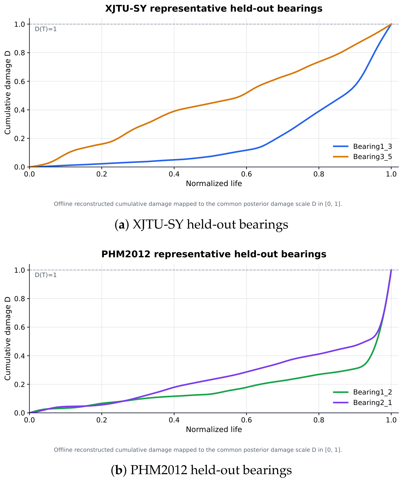
Equations (7)–(9) define the study-specific transformation from the offline PCA-HI to the normalized posterior cumulative damage coordinate. Damage statistics from the preprocessing stage show that the monotonicity of both datasets is 1.0, the terminal error is 0, and the increment-sum error is close to 0. Figure 3 shows representative offline-reconstructed damage coordinates for held-out bearings. The horizontal axis is normalized life, and the vertical axis is cumulative damage D in the posterior damage coordinate. This step maps bearings with different lengths, operating conditions, and degradation rates to the posterior damage scale from $D=0$ to $D=1$, providing the basis for probabilistic threshold-crossing assessment.

2.6. Deep Sequence-Parameterized Gamma Damage Process Model

On the basis of the cumulative damage sequence, windows of the damage process are constructed as deep-model inputs. At time t, the model input includes cumulative damage $D\left(t\right)$, damage increment $\Delta D\left(t\right)$, local velocity $v\left(t\right)$, local acceleration $a\left(t\right)$, and fast degradation score $s_f\left(t\right)$:

$$\mathbf{u}\left(t\right)=\left[D\left(t\right),\Delta D\left(t\right),v\left(t\right),a\left(t\right),s_f\left(t\right)\right].$$

(10)

Using the length-L window ${\mathbf{U}}_{t-L+1:t}$ as input, the deep sequence network outputs the Gamma distribution parameters of the next damage increment, a life-label auxiliary output, and a fast-degradation-state auxiliary output. Transformer-GRU is used as the pre-specified default sequence parameterizer. The Transformer attention structure extracts short- and long-term dependencies within the input window [34], while Transformer-only and GRU-only are compared in the backbone ablation to distinguish the contribution of the network structure from those of the probabilistic damage process and Bayesian updating modules. The window length is 32 with stride 1 for XJTU-SY and 64 with stride 5 for PHM2012; the hidden dimension is 64, the number of attention heads is 4, the number of training epochs is 20, and the number of Monte Carlo paths is 1000. 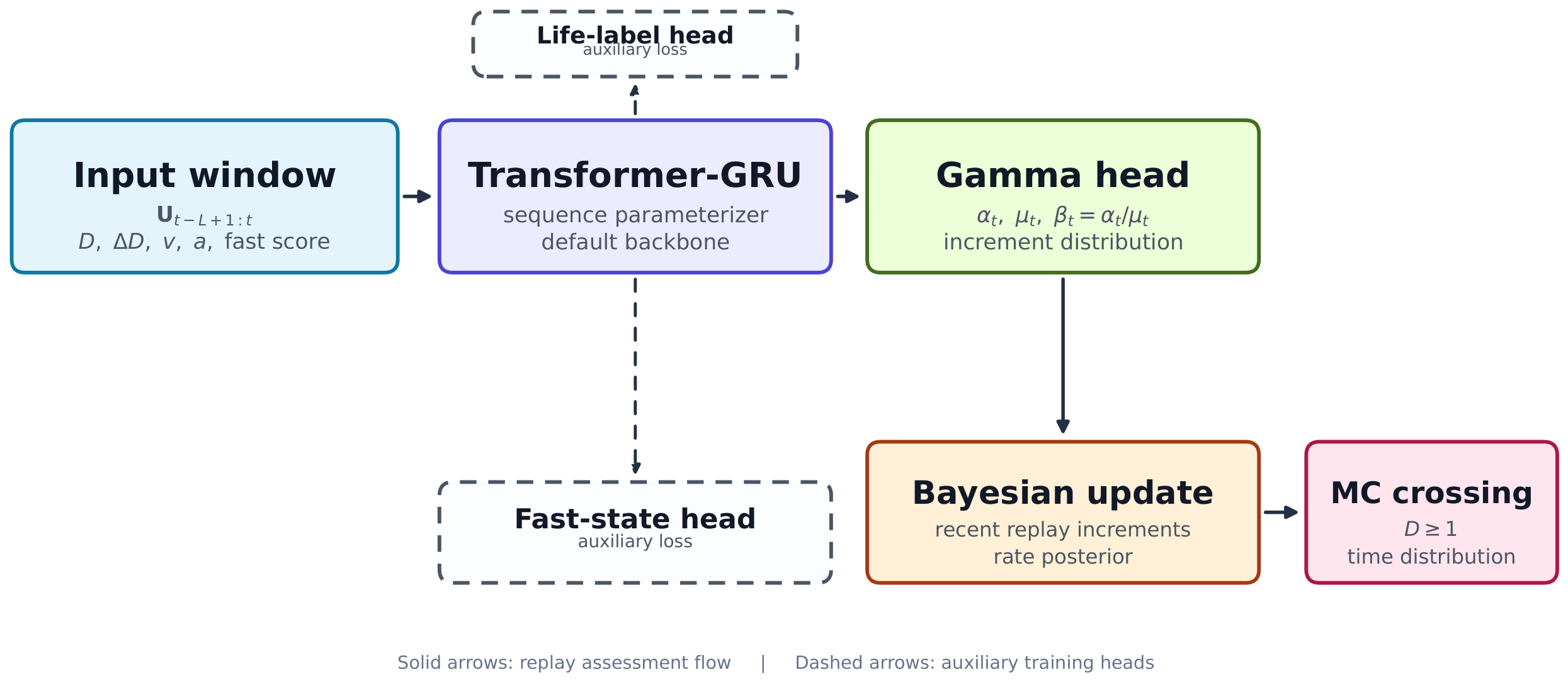Figure 4 shows the architecture of the deep Gamma damage process model, in which Transformer-GRU is used as the default sequence parameterizer.

Let the network output the damage-increment mean ${\mu }_t$ and shape parameter ${\alpha }_t$. Throughout this study, $\mathrm{Gamma}(\alpha ,\beta )$ denotes the shape–rate distribution, whose mean and variance are $\alpha /\beta$ and $\alpha /{\beta }^2$, respectively; $\beta$ is therefore a rate parameter rather than a scale parameter. The rate parameter is then

$${\beta }_t={\displaystyle \frac{{\alpha }_t}{{\mu }_t}}.$$

(11)

The next damage increment follows

$$\Delta D(t+1)\sim \mathrm{Gamma}({\alpha }_t,{\beta }_t),$$

(12)

with mean and variance given by

$$\mathrm{E}[\Delta D(t+1)]={\displaystyle \frac{{\alpha }_t}{{\beta }_t}},\mathrm{Var}[\Delta D(t+1)]={\displaystyle \frac{{\alpha }_t}{{\beta }_t^2}}.$$

(13)

The network loss consists of the Gamma negative log-likelihood, a damage-increment mean constraint, a life-label constraint, a threshold-consistency constraint, and an auxiliary fast-degradation-state loss. The life-label constraint encourages the model to learn the linear relation $1-\mathrm{RUL}/\mathrm{life}$, and the threshold-consistency constraint links the predicted increment, remaining damage, and estimated remaining steps. The main implementation details are summarized in

Table 3. Implementation details and hyperparameter settings of the offline replay and truncation experiments.

Parameter	XJTU-SY	PHM2012
Input window length/stride	32/1	64/5
Default backbone	Transformer-GRU; compared with Transformer-only and GRU-only	Transformer-GRU; compared with Transformer-only and GRU-only
Hidden dimension/attention heads/layers	64/4/1	64/4/1
Dropout	0.1	0.1
Optimizer	AdamW, learning rate 0.001, weight decay ${10}^{-4}$	AdamW, learning rate 0.001, weight decay ${10}^{-4}$
Batch size/epochs	256/20	256/20
Mean-increment constraint weight	0.02	0.02
Life-label/threshold/fast-state weights	0.5/2.0/0.05	0.5/2.0/0.05
Bayesian window/fast window	24/8	24/6
Bayesian prior strength, base/fast state	30/15	30/15
Gamma variance inflation factor	3	3
Failure threshold/Monte Carlo paths	$D=1$, 1000 paths	$D=1$, 1000 paths
Hardware	CUDA GPU	CUDA GPU

. The computational workflow was implemented using Python 3.9.25, PyTorch 2.5.1, NumPy 1.26.4, SciPy 1.13.1, scikit-learn 1.5.1, pandas 2.3.3, and Matplotlib 3.9.4.

The reported hyperparameter configuration was fixed before the final tables were generated and was not adjusted according to test-bearing crossing-time errors. Because no independent validation bearing was used and the best epoch was selected by the holdout next-step increment metric from training-bearing windows, this setting remains a methodological limitation. Independent validation bearings, leave-one-bearing-out validation, or nested validation would provide a stricter robustness assessment.

2.7. Rolling Bayesian Updating and Posterior Fast-Degradation-State Usage

When only the trained deep-model prior is used, the response to rapid degradation in a test bearing may lag. Rolling Bayesian rate updating is therefore introduced during the replay stage. Under the stated shape–rate convention for the Gamma prior on the rate, the conjugate update follows the standard Bayesian formulation [35]. Let the prior mean provided by the model at time t be ${\overline{\beta }}_t$, the rate variable to be updated be $\beta$, and the prior strength be $c_0$. Then

$$\beta \sim \mathrm{Gamma}(c_0,d_0),d_0={\displaystyle \frac{c_0}{{\overline{\beta }}_t}}.$$

(14)

If the damage increments in the most recent m windows satisfy

$$\Delta D_i\mid \beta \sim \mathrm{Gamma}({\alpha }_i,\beta ),i=1,\dots ,m,$$

(15)

then, when ${\alpha }_i$ varies with time, the posterior distribution of the rate parameter is

$$\beta \mid {\{\Delta D_i\}}_{i=1}^m\sim \mathrm{Gamma}\left(c_0+{\displaystyle \sum _{i=1}^m}{\alpha }_i,d_0+{\displaystyle \sum _{i=1}^m}\Delta D_i\right).$$

(16)

A local stationary approximation is used by assuming ${\alpha }_i\approx {\alpha }_t$ within the recent window. The posterior mean of the rate can therefore be written as

$${\widehat{\beta }}_t={\displaystyle \frac{c_0+m{\alpha }_t}{d_0+{\sum }_{i=1}^m\Delta D_i}}.$$

(17)

The complete posterior predictive distribution over $\beta$ is not analytically integrated. Instead, a posterior-mean plug-in approximation is adopted:

$$\Delta D(t+1)\mid {\mathcal{D}}_t\approx \mathrm{Gamma}({\alpha }_t,{\widehat{\beta }}_t).$$

(18)

Here, ${\mathcal{D}}_t$ denotes the damage observations available before the current replay time t, specifically the offline reconstructed damage increments within the current Bayesian window. When the bearing enters the fast-degradation state, the Bayesian window is shortened and the prior strength is reduced, so that recent observed increments receive a higher weight in extrapolation. The base Bayesian window is 24; the fast window is 8 for XJTU-SY and 6 for PHM2012. The base prior strength is 30, and with fast-state gain 1.0 it is reduced to 15 when the fast-state indicator equals 1 at zero lag; during future extrapolation it can be further weakened by the lag-dependent boost. The update is therefore a posterior correction in offline rolling replay rather than future-independent online inference. A systematic sensitivity analysis of the Bayesian window, prior strength, and variance inflation factor is not included in the main tables, and the selected configuration may be dataset-dependent.

Fast-degradation identification is adapted from the adaptive threshold method based on rate of change (ATMROC) proposed by Liu et al. [36]. In the present study, the sliding rate-of-change criterion is applied to the offline reconstructed cumulative damage coordinate rather than directly to a health indicator. The thresholding rule is further modified using healthy-baseline statistics, robust dispersion measures, a global quantile, and a sustained-trigger condition. To avoid ambiguity between offline and prefix-available meanings, two types of rate of change are distinguished. Offline label construction uses the forward rate of change from the complete trajectory:

$${\mathrm{ROC}}_{\mathrm{offline}}\left(t\right)={\displaystyle \frac{\max (0,D(t+w)-D(t\left)\right)}{w}},$$

(19)

This quantity is used for full-life trajectory analysis and auxiliary fast-degradation label generation. In strict truncation or deployment-oriented settings, only the past-window rate of change can be used:

$${\mathrm{ROC}}_{\mathrm{past}}\left(t\right)={\displaystyle \frac{\max (0,D(t)-D(t-w\left)\right)}{w}}.$$

(20)

The threshold is determined jointly by the healthy-baseline mean, standard deviation, median, MAD, and global quantile. When the rate of change continuously exceeds the threshold and cumulative damage leaves the low-damage plateau, the fast-degradation label is set to 1. In these experiments, the fast-degradation label and fast score are constructed from ${\mathrm{ROC}}_{\mathrm{offline}}\left(t\right)$. During rolling replay, the fast score in the input window also comes from the already offline reconstructed complete damage trajectory and, together with the network-predicted fast state, triggers Bayesian-window adjustment. Therefore, the fast score is a posterior explanatory feature, not a strictly prefix-available online feature. The resulting interpretation is restricted to posterior explanation from complete trajectories and rolling-replay assessment. The sources of fast-degradation variables at different stages are listed in

Table 4. Sources and uses of fast-degradation variables at different stages.

Stage	Variable Source	Uses Future Damage Value?	Use and Interpretation
Training label	${\mathrm{ROC}}_{\mathrm{offline}}\left(t\right)$ with sustained-threshold rule	Yes	Generates the auxiliary fast-state label and the fast score
Replay input	Offline fast score predicted fast state	Yes, under the offline posterior replay setting only	Posterior replay feature shortens the Bayesian window and strengthens recent increments
Strict truncation/ online setting	${\mathrm{ROC}}_{\mathrm{past}}\left(t\right)$ or predicted fast state	No	Uses prefix-available variables not covered by the current replay protocol

.

2.8. Offline Rolling Replay Protocol and Evaluation Metrics

The experiments use an offline rolling replay protocol. First, PCA-HI and cumulative damage trajectories are constructed offline from the complete life vibration records of the test bearings. The rolling assessment then starts from a fixed-length window, with an initial window of 32 sample segments for XJTU-SY and 64 sample segments for PHM2012. Within the true trajectory length, the model replays the reconstructed true damage prefix segment by segment; rolling Bayesian updating uses the true increments before the current replay time, whereas the true endpoint after the replay time is used only for evaluating error and coverage.

Table 5. Statistical unit of the fixed-initial-window offline rolling replay demonstration.

Dataset	Initial-Window End ${\mathit{t}}_0$	Replay Step	Starts per Bearing	Excludes the Late Pre-Failure Segment
XJTU-SY	$L-1=31$	1 sample segment	1	No; replay proceeds along the complete offline trajectory until threshold crossing
PHM2012	$L-1=63$	1 sample segment	1	No; replay proceeds along the complete offline trajectory until threshold crossing

gives the statistical unit of the fixed-initial-window demonstration. In this setup, each bearing and random seed in

Table 6. Fixed-initial-window offline rolling replay demonstration of the proposed method.

Dataset	Test Bearing	Median Crossing-Time MAE	PICP90	MPIW90
XJTU-SY	Bearing1_1	$1.000\pm 0.000$	1.00	21.61
	Bearing1_3	$0.600\pm 0.548$	1.00	13.80
	Bearing2_2	$1.300\pm 1.204$	1.00	24.62
	Bearing3_5	$1.400\pm 0.548$	1.00	20.41
	Average	$1.075\pm 0.730$	1.00	20.11
PHM2012	Bearing1_2	$1.600\pm 0.894$	1.00	43.24
	Bearing2_1	$0.400\pm 0.548$	1.00	39.20
	Bearing2_2	$0.800\pm 0.447$	1.00	43.05
	Bearing2_4	$0.400\pm 0.894$	1.00	41.03
	Average	$0.800\pm 0.834$	1.00	41.63

Note: Bearing rows report mean ± standard deviation over five random seeds for the corresponding bearing. Average rows report pooled mean ± standard deviation over 20 bearing-seed samples. Each bearing-seed pair yields one final crossing-time distribution after fixed-initial-window replay. MPIW90 is the mean of $Q_{0.95}-Q_{0.05}$ in sample segments.

produces only one crossing-time distribution. The MAE is not an average over multiple replay starts; instead, it represents the final crossing-time distribution error after starting from a fixed initial window and then replaying along the complete offline damage trajectory. Fixed-ratio truncation experiments at 20%, 40%, 60%, and 80% are used to assess stage-wise extrapolation under the same offline damage coordinate. The true damage increments after the truncation point are not used in Bayesian updating. In the fixed-ratio truncation experiment, the fast-state variable follows the same offline posterior setting as Table 4 and is not treated as prefix-available. If a fast-degradation state is needed under a prefix-available setting, ${\mathrm{ROC}}_{\mathrm{past}}$ or a predicted fast state would have to be used. This experiment is therefore an offline truncation analysis rather than a strict online protocol.

At each rolling time, the model iteratively samples the next damage increment and accumulates the increments to obtain predicted damage paths. The first time at which each Monte Carlo path satisfies

$$D\left(t\right)\ge 1$$

(21)

is defined as the assessed threshold-crossing time of that path. The 1000 paths provide the median crossing time, 5% quantile, 95% quantile, and cumulative distribution probability before the true failure time. The sample-segment index denotes the chronological order of the vibration records. One index step corresponds to 1 min for XJTU-SY and 10 s for PHM2012. The crossing-time PDF represents the probability density estimated from the first threshold-crossing indices of the 1000 Monte Carlo paths. The main metrics for posterior crossing-time assessment are median-time mean absolute error (MAE), root mean squared error (RMSE), 90% prediction interval coverage probability (PICP90), and 90% mean prediction interval width (MPIW90):

$$\mathrm{MAE}={\displaystyle \frac{1}{n}}{\displaystyle \sum _{i=1}^n}|{\widehat{T}}_i-T_i|,\mathrm{RMSE}=\sqrt{{\displaystyle \frac{1}{n}}\sum _{i=1}^n{({\widehat{T}}_i-T_i)}^2}.$$

(22)

where $T_i$ is the true failure time and ${\widehat{T}}_i$ is the median of the assessed crossing-time distribution. Let the 5% and 95% quantiles of the ith sample be $Q_{0.05,i}$ and $Q_{0.95,i}$, respectively. Then

$$\begin{array}{cc}\hfill {\mathrm{PICP}}_{90}& ={\displaystyle \frac{1}{n}}{\displaystyle \sum _{i=1}^n}1\left(Q_{0.05,i}\le T_i\le Q_{0.95,i}\right),\hfill \\ \hfill {\mathrm{MPIW}}_{90}& ={\displaystyle \frac{1}{n}}{\displaystyle \sum _{i=1}^n}\left(Q_{0.95,i}-Q_{0.05,i}\right).\hfill \end{array}$$

(23)

PICP90 reflects interval coverage, whereas MPIW90 reflects interval width. These two quantities are interpreted jointly to avoid obtaining high coverage only through excessively wide intervals. The fixed-ratio truncation experiment also reports the coverage rates at 50%, 70%, 90%, and 95% confidence levels and the normalized interval width

$${\mathrm{nMPIW}}_{90}={\displaystyle \frac{1}{n}}{\displaystyle \sum _{i=1}^n}{\displaystyle \frac{Q_{0.95,i}-Q_{0.05,i}}{T_i}},$$

(24)

as well as the continuous ranked probability score (CRPS). Given the Monte Carlo failure-time samples ${\left\{x_{i,m}\right\}}_{m=1}^M$ and the true failure time $T_i$ of the ith sample, the empirical CRPS is calculated as

$${\mathrm{CRPS}}_i={\displaystyle \frac{1}{M}}{\displaystyle \sum _{m=1}^M}|x_{i,m}-T_i|-{\displaystyle \frac{1}{2M^2}}{\displaystyle \sum _{m=1}^M}{\displaystyle \sum _{\ell =1}^M}|x_{i,m}-x_{i,\ell }|.$$

(25)

A smaller CRPS indicates that the assessed distribution is closer to the true failure time [37]. The XJTU-SY test bearings are Bearing1_1, Bearing1_3, Bearing2_2, and Bearing3_5, whereas the PHM2012 test bearings are Bearing1_2, Bearing2_1, Bearing2_2, and Bearing2_4. The fixed-initial-window replay demonstration, fixed-ratio truncation experiments, method comparisons, and ablation experiments use five random seeds.

3. Results

The results are reported in two layers. The fixed-initial-window replay results in Table 6 and Figure 5 and Figure 6 are controlled offline posterior replay demonstrations and are not used to claim calibrated early-stage prefix prediction. The fixed-ratio truncation experiment in

Table 7. Fixed-ratio truncation results and probabilistic scores used as the primary applicability-boundary test.

(a) XJTU-SY
Truncation	MAE	RMSE	PICP50	PICP70	PICP90	PICP95	MPIW90	nMPIW90	CRPS
20%	154.8	252.6	0.30	0.35	0.65	0.70	430.9	2.93	124.1
40%	100.4	129.9	0.10	0.30	0.50	0.55	266.5	1.89	75.3
60%	60.5	78.1	0.20	0.35	0.40	0.55	170.1	1.24	46.3
80%	11.5	14.8	0.35	0.45	0.80	0.85	49.5	0.35	8.4
(b) PHM2012
20%	523.6	537.1	0.00	0.00	0.30	0.40	426.7	0.52	471.8
40%	400.9	402.8	0.00	0.00	0.25	0.40	286.4	0.35	357.2
60%	240.5	241.9	0.00	0.00	0.30	0.40	238.7	0.29	207.0
80%	79.8	81.1	0.00	0.10	0.60	0.90	287.6	0.35	57.7

Note: Each row contains 20 samples, i.e., 4 test bearings × 5 random seeds. CRPS and time errors are reported in sample segments; nMPIW90 is MPIW90 normalized by the true failure time. The fixed-ratio truncation experiment is not interpreted as a strict online deployment protocol because the damage coordinate itself is constructed offline from the full trajectory.

and Figure 7 is the primary evidence for applicability boundaries. The method comparison in

Table 8. Comparison of probabilistic crossing-time assessment methods under the fixed-initial-window offline replay demonstration. Values are reported as mean ± standard deviation of dataset-level averages over five random seeds.

Dataset	Method	MAE	RMSE	PICP90	MPIW90
XJTU-SY	Proposed	$1.075\pm 0.527$	$1.219\pm 0.468$	1.00	20.11
	Isotonic–Gamma	$31.000\pm 0.342$	$31.702\pm 0.325$	0.70	74.43
	Two-Phase Gamma	$10.850\pm 0.285$	$13.131\pm 0.192$	0.60	29.07
	Bayesian Gamma	$6.775\pm 0.137$	$9.075\pm 0.051$	0.75	22.00
	Adaptive Wiener	$16.325\pm 0.112$	$16.892\pm 0.115$	0.00	15.65
	MC Dropout GRU	$5.025\pm 0.224$	$5.841\pm 0.243$	0.75	13.25
PHM2012	Proposed	$0.800\pm 0.209$	$1.137\pm 0.093$	1.00	41.63
	Isotonic–Gamma	$23.975\pm 1.216$	$26.291\pm 1.384$	1.00	121.90
	Two-Phase Gamma	$54.875\pm 0.331$	$76.598\pm 0.384$	0.50	111.32
	Bayesian Gamma	$9.050\pm 0.274$	$15.088\pm 0.696$	0.95	76.58
	Adaptive Wiener	$18.600\pm 0.137$	$18.625\pm 0.143$	0.00	18.90
	MC Dropout GRU	$8.275\pm 0.137$	$8.342\pm 0.144$	0.20	12.60

Note: The standard deviations in this table are computed at the seed level and are therefore not directly comparable with the pooled bearing-seed standard deviations in Table 6. PICP90 and MPIW90 are averaged over the combined bearing and seed samples. Bold values indicate the proposed method and its corresponding results.

is also reported under the fixed-initial-window offline replay protocol.

3.1. Fixed-Initial-Window Offline Rolling Replay Demonstration

Table 6 reports the median threshold-crossing-time errors, coverage rates, and interval widths of the fixed-initial-window offline rolling replay demonstration over five random seeds. Bearing-specific MAE entries are summarized over the five seeds for each test bearing, whereas the Average rows pool the four test bearings and five seeds, yielding 20 bearing-seed samples per dataset. The pooled MAE values are $1.075\pm 0.730$ sample segments for XJTU-SY and $0.800\pm 0.834$ sample segments for PHM2012. PICP90 is 1.0 on both datasets, and the corresponding MPIW90 values are 20.11 and 41.63 sample segments. These results belong to the fixed-initial-window replay setting and are not used as calibration evidence for the fixed-ratio truncation experiment.

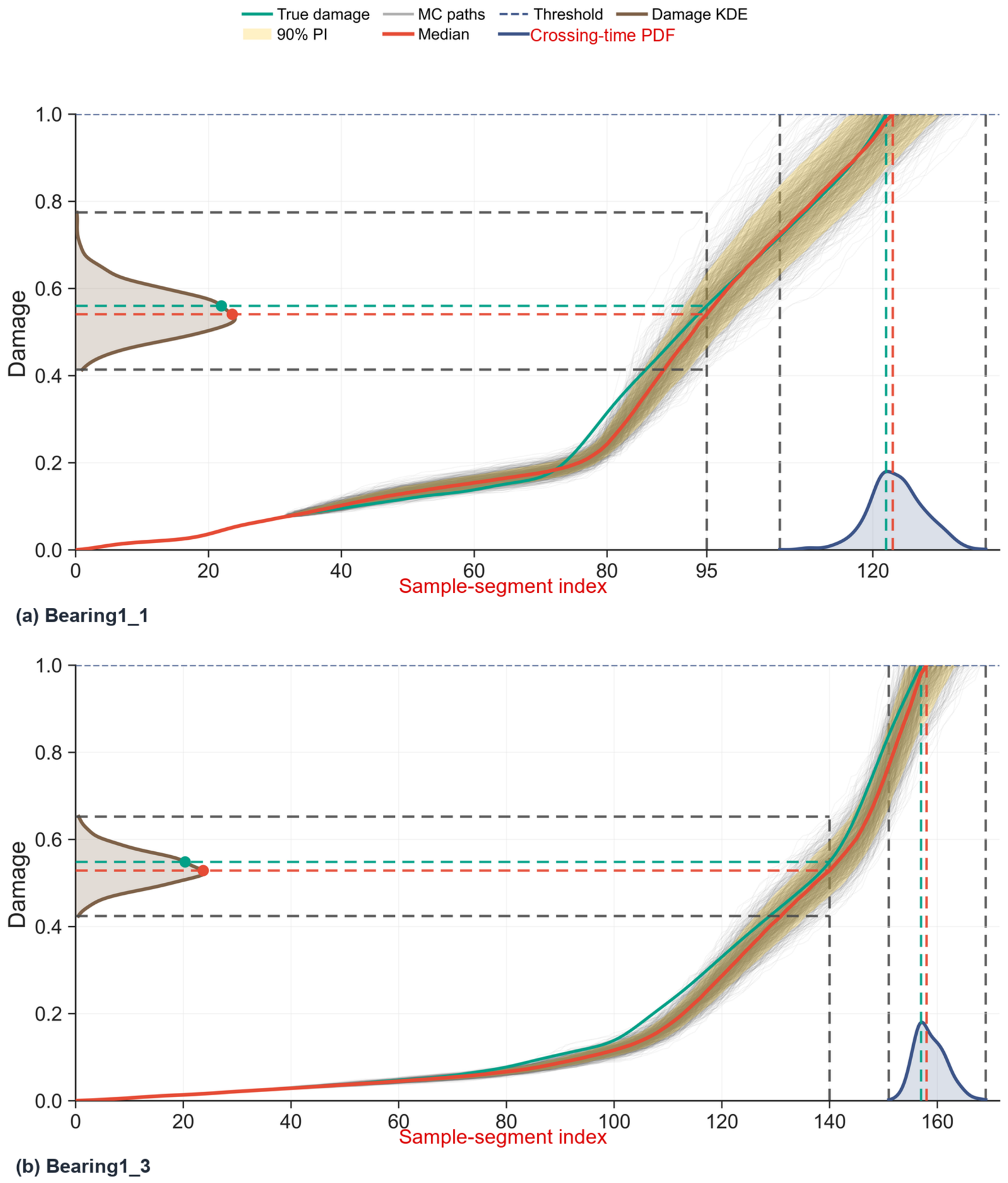
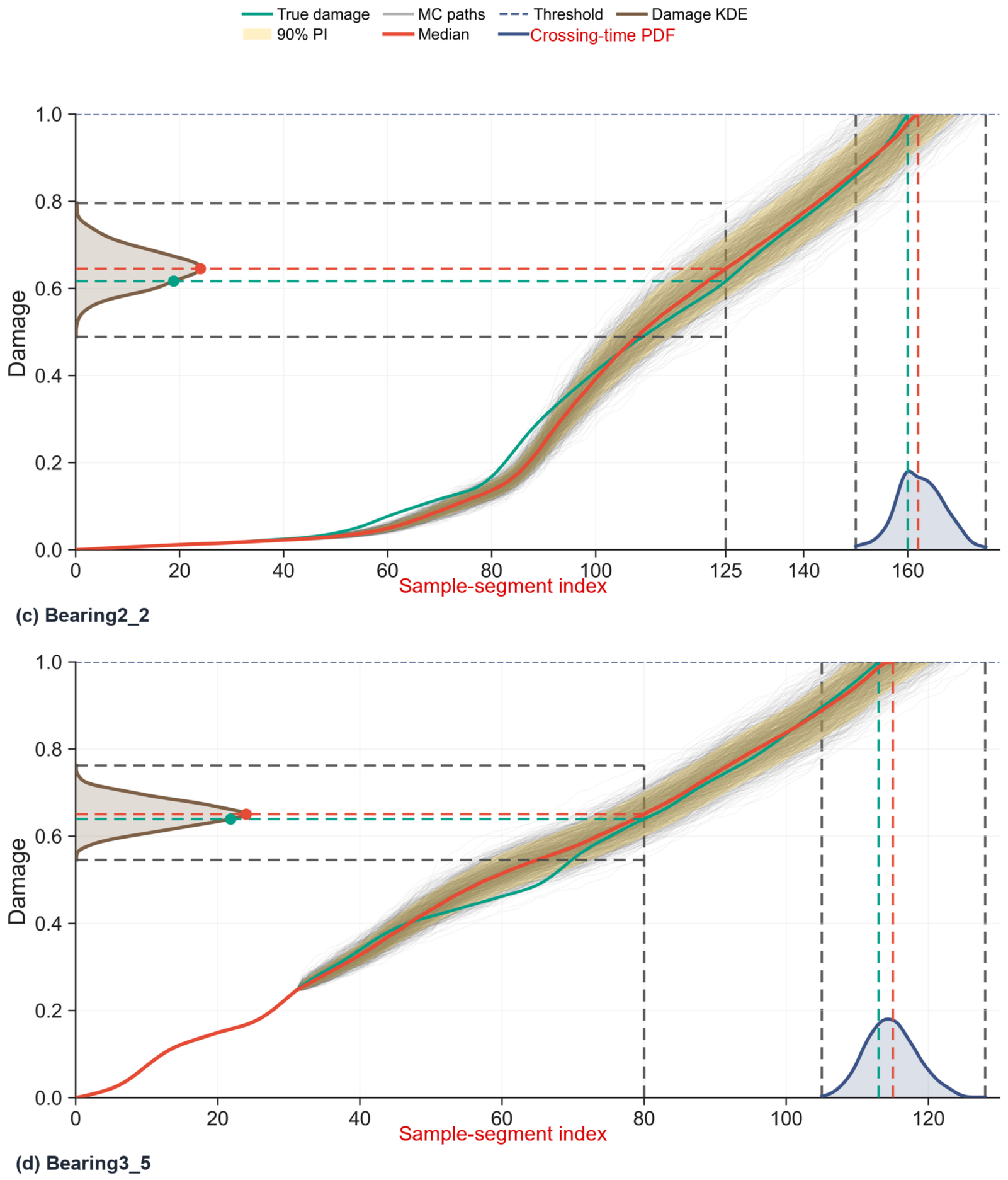
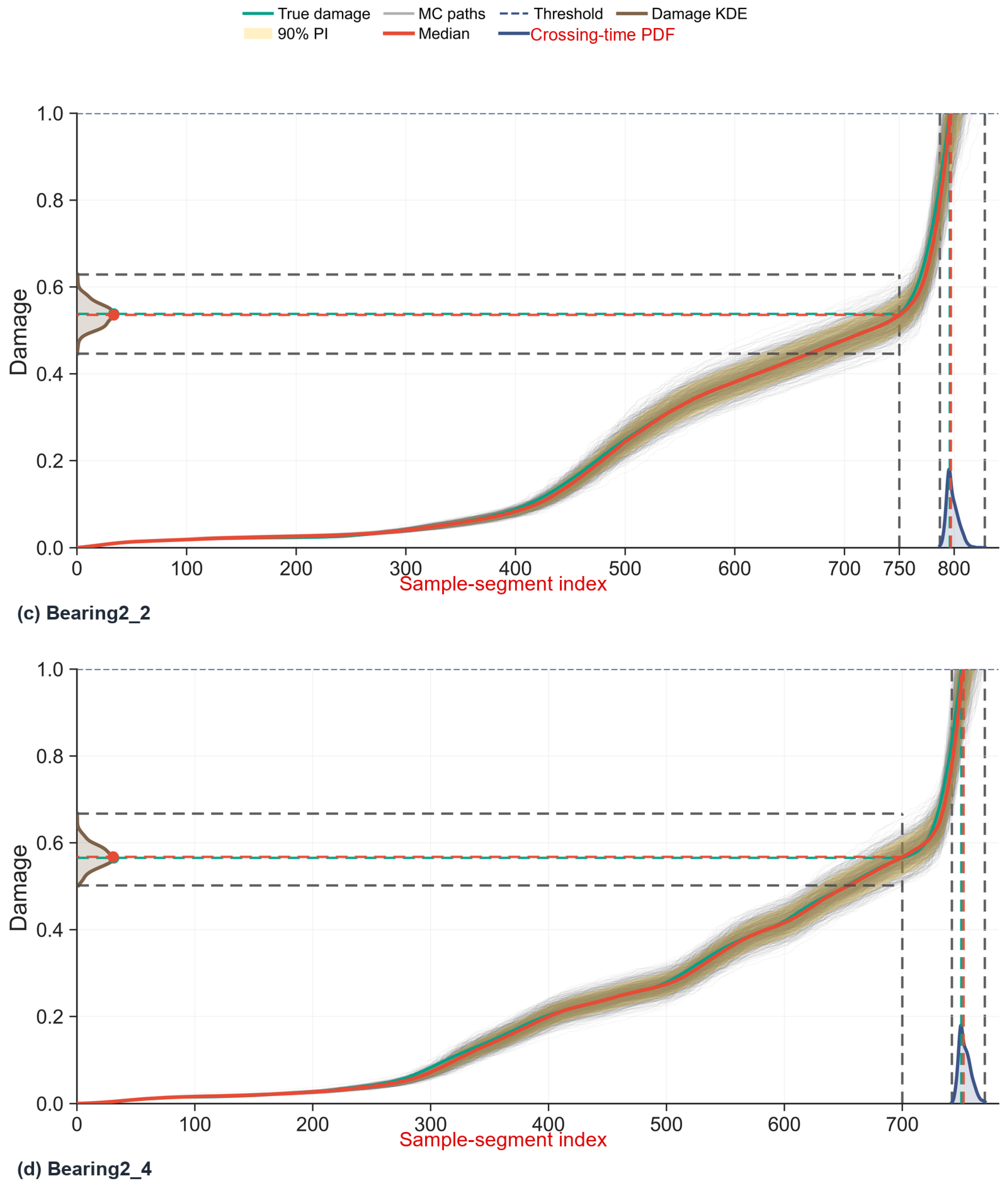
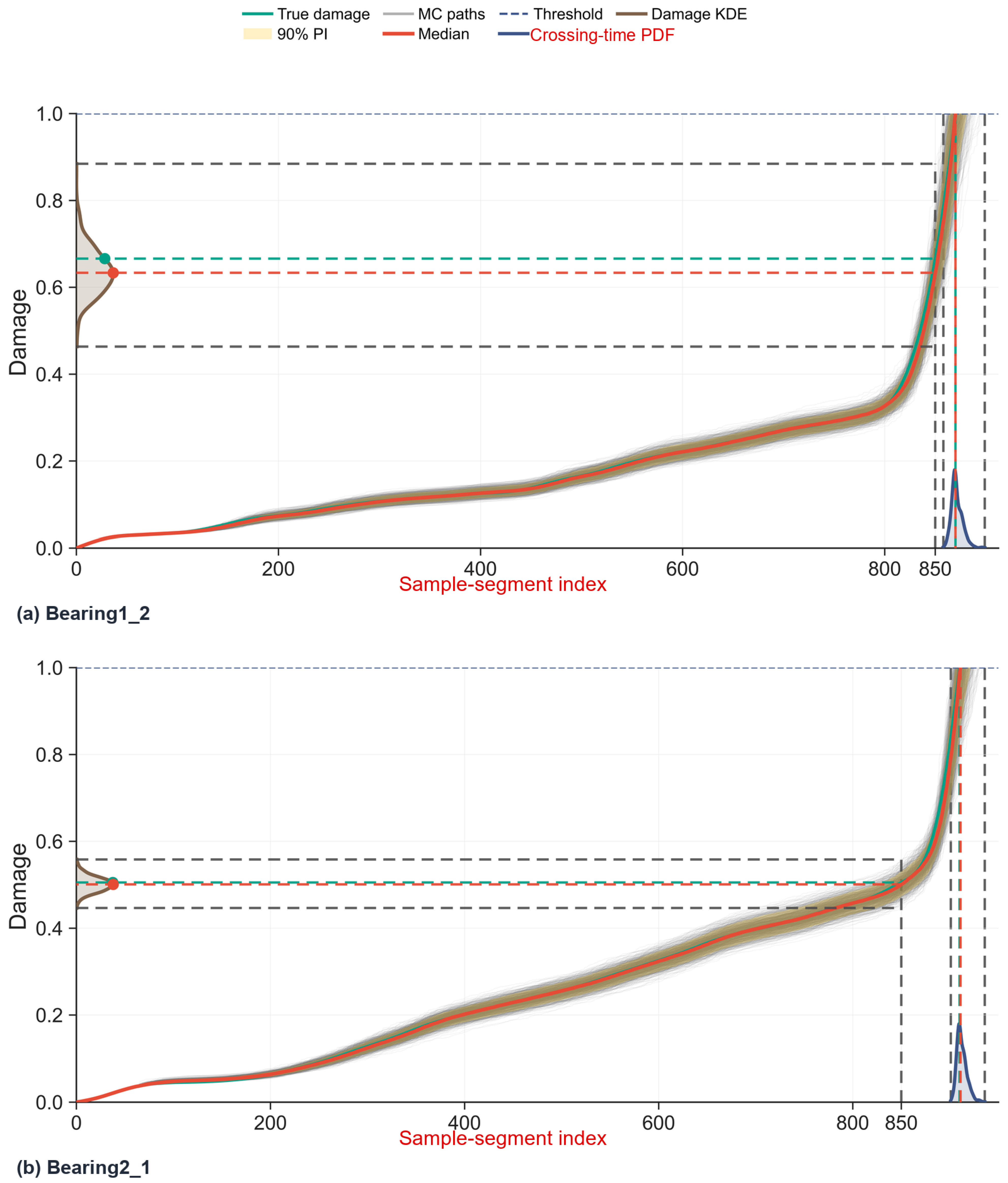
Figure 5 and Figure 6 show offline rolling replay curves for all four test bearings of XJTU-SY and all four test bearings of PHM2012 under seed_3, respectively. This seed is selected for visualization because the prediction paths, 90% intervals, crossing-time PDF curves, and damage-section KDEs are all clearly displayed for the two datasets. The true damage curve, Monte Carlo paths, crossing-time distribution, and damage-section distribution jointly illustrate the probabilistic extrapolation process in the posterior damage coordinate. The left-side damage-section KDE represents the kernel density estimate of Monte Carlo cumulative damage samples at a selected replay section. The red dashed line denotes the median sampled damage, the cyan dashed line denotes the reconstructed damage at that section, and the gray dashed lines denote the 5% and 95% damage quantiles. It visualizes local cumulative damage uncertainty, whereas the right-side crossing-time PDF summarizes threshold-crossing-time uncertainty. Replay starts after the fixed initial window, with $L-1=31$ for XJTU-SY and $L-1=63$ for PHM2012. The horizontal axis is the sample-segment index. The true failure time, median crossing time, 5%/95% quantiles, and 90% interval are used to interpret interval coverage. The figures present the fixed-initial-window replay demonstration for all test bearings; extrapolation at different degradation stages is evaluated separately by the fixed-ratio truncation experiment in Table 7. PHM2012 generally has wider intervals than XJTU-SY, which is associated with its longer life length, more end-of-life concentrated degradation, and stronger local fluctuations.

3.2. Fixed-Ratio Truncation as the Primary Applicability-Boundary Test

Because the fixed-initial-window replay demonstration may not reflect stage-wise extrapolation difficulty, fixed-ratio truncation is used as the primary experiment for assessing applicability boundaries. Truncation experiments are conducted at 20%, 40%, 60%, and 80%. For each test bearing and random seed, the offline damage trajectory is truncated at the ratio $r{T}_i$ of the true failure time $T_i$. The model uses only the damage prefix and network state at or before the truncation point for Monte Carlo extrapolation, and the true damage increments after the truncation point are not used in rolling Bayesian updating. The fast-state variable in this truncation experiment follows the offline posterior setting defined in Table 4; it is not a ${\mathrm{ROC}}_{\mathrm{past}}$ or purely predicted fast-state comparison. Table 7 presents the pooled statistics from 4 test bearings × 5 random seeds. This test remains based on the offline constructed damage coordinate and is used to characterize posterior prefix extrapolation rather than online deployment.

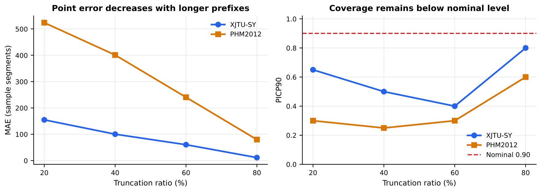
Figure 7 summarizes the trend of the primary applicability-boundary test. The fixed-ratio truncation results indicate that the model performs substantially better when a sufficient middle-to-late damage prefix is available. For XJTU-SY, PICP90 values at 20%, 40%, 60%, and 80% truncation are 0.65, 0.50, 0.40, and 0.80, respectively. The corresponding PHM2012 values are 0.30, 0.25, 0.30, and 0.60. These values are well below the nominal 0.90 coverage level, especially for early and middle-stage PHM2012 prefixes, where uncertainty is strongly underestimated. Thus, the fixed-ratio truncation experiment reveals both point-estimation errors and severe interval undercoverage. The PICP90 = 1.0 observed in the fixed-initial-window replay demonstration applies only to that posterior replay setting and does not represent probability calibration under truncation-based extrapolation. Table 7 therefore provides the main evidence for the current method’s applicability boundary, whereas Table 6 reports a controlled offline replay demonstration.

3.3. Method-Comparison Results

To compare method behavior under the controlled posterior replay setting, the deep Gamma damage process is compared with five classes of methods: Isotonic–Gamma, Two-Phase Gamma, Bayesian Gamma, Adaptive Wiener, and MC Dropout GRU. The method comparison is conducted under the fixed-initial-window replay protocol, whereas the fixed-ratio truncation experiment is used to characterize applicability boundaries. Isotonic–Gamma first smooths cumulative damage through isotonic regression and then extrapolates the failure time with a single-stage Gamma process. Two-Phase Gamma estimates slow and fast two-stage Gamma processes according to the fast-degradation boundary of the training bearings. Bayesian Gamma uses damage-stage Gamma parameters from training bearings and adopts the same rolling Bayesian rate updating and fast window as the proposed method, but it does not use a deep sequence network to output increment parameters. Adaptive Wiener trains drift and diffusion terms and performs Wiener extrapolation with the observed window of the test bearing. MC Dropout GRU uses a GRU increment estimator and inference-time Dropout sampling to estimate probabilistic failure time [38].

To maintain a consistent comparison protocol, all methods use the same offline cumulative damage $D\left(t\right)$ and damage increment $\Delta D\left(t\right)$ obtained from the damage-construction stage, the same test-bearing split, the same five random seeds, and the same true threshold-crossing criterion. The offline reconstructed damage prefix of the test bearing is permitted for rolling replay. Bayesian Gamma shares the Bayesian rate updating and fast window with the proposed method, enabling the contribution of deep increment parameterization to be separated from that of observation-based posterior correction. The conventional Gamma/Wiener baselines do not use time-varying increment distributions output by a deep network. Table 8 therefore compares the complete framework with several interpretable baselines within the fixed-initial-window replay protocol.

Table 8 shows that, under the fixed-initial-window offline rolling replay demonstration, the proposed method obtains the lowest median crossing-time MAE and RMSE on both datasets. On XJTU-SY, the proposed method has an MAE of $1.075\pm 0.527$, which is lower than $5.025\pm 0.224$ for MC Dropout GRU, $6.775\pm 0.137$ for Bayesian Gamma, and $10.850\pm 0.285$ for Two-Phase Gamma. On PHM2012, the proposed method has an MAE of $0.800\pm 0.209$, which is also lower than those of the comparison methods. The MAE values of Bayesian Gamma are $6.775\pm 0.137$ on XJTU-SY and $9.050\pm 0.274$ on PHM2012, indicating that the same Bayesian updating reduces traditional Gamma extrapolation errors in these experiments, but remains weaker than the complete method without deep time-varying increment parameterization. PICP90 and MPIW90 further show that some baselines have narrow intervals but low coverage. Bayesian Gamma reaches a PICP90 of 0.95 on PHM2012, but its MPIW90 is 76.58, wider than the 41.63 of the proposed method. These comparisons apply to the posterior replay protocol and are separate from the stricter fixed-ratio truncation setting.

3.4. Key-Module Ablation Experiments

Table 9. Ablation results for key modules. Values are reported as mean ± standard deviation of dataset-level averages over five random seeds.

Dataset	Setting	MAE	RMSE	PICP90	MPIW90
XJTU-SY	Full method	$1.075\pm 0.527$	$1.219\pm 0.468$	1.00	20.11
	Without Bayesian update	$17.975\pm 17.660$	$21.708\pm 21.413$	0.55	43.66
	Without posterior fast-state usage	$9.550\pm 0.716$	$10.306\pm 0.417$	0.40	67.87
	Without uncertainty calibration	$1.800\pm 0.622$	$1.951\pm 0.490$	1.00	11.45
PHM2012	Full method	$0.800\pm 0.209$	$1.137\pm 0.093$	1.00	41.63
	Without Bayesian update	$24.450\pm 20.077$	$26.724\pm 20.907$	0.55	174.23
	Without posterior fast-state usage	$18.650\pm 1.719$	$18.999\pm 1.931$	0.45	194.82
	Without uncertainty calibration	$1.925\pm 0.622$	$2.046\pm 0.533$	1.00	11.95

Note: The MAE/RMSE standard deviation is computed from dataset-level averages over five random seeds. PICP90 and MPIW90 are averaged over the combined bearing and seed samples. Bold values indicate the full method and its corresponding results.

presents the key-module ablation results under the fixed-initial-window offline replay demonstration. Without rolling Bayesian updating, the MAE increases from $1.075\pm 0.527$ to $17.975\pm 17.660$ on XJTU-SY and from $0.800\pm 0.209$ to $24.450\pm 20.077$ on PHM2012, while interval coverage drops to 0.55. This result indicates that recent observed increments in the offline reconstructed damage prefix of the test bearing provide a key constraint for posterior replay extrapolation. Without posterior fast-degradation-state usage, the MAE increases to $9.550\pm 0.716$ on XJTU-SY and $18.650\pm 1.719$ on PHM2012, and MPIW90 increases to 67.87 and 194.82, respectively. The posterior fast-degradation state therefore helps shorten the Bayesian window before failure and increases the weight of recent observations, reducing lag and excessively wide intervals. Because the fast score is constructed from ${\mathrm{ROC}}_{\mathrm{offline}}\left(t\right)$, these ablation results constitute mechanism evidence inside the offline posterior replay protocol rather than evidence of an online fast-state module.

Additional life-label sensitivity checks were dataset-dependent and are therefore not treated as a core effective-module ablation in Table 9. Removing additional variance inflation increases the MAE on both datasets but produces narrower MPIW90 values. Thus, variance calibration affects both median-time error and interval width, defining an explicit median-error and interval-width trade-off.

3.5. Backbone-Module Ablation and Significance Testing

The backbone-module ablation results are shown in

Table 10. Backbone-module ablation results. Values are reported as mean ± standard deviation of dataset-level averages over five random seeds. Transformer-GRU is retained as the pre-specified default parameterizer.

Dataset	Backbone	MAE	RMSE	PICP90	MPIW90
XJTU-SY	Transformer-GRU	$1.075\pm 0.527$	$1.219\pm 0.468$	1.00	20.11
	GRU-only	$1.700\pm 1.052$	$1.967\pm 0.955$	1.00	42.91
	Transformer-only	$0.700\pm 0.209$	$0.874\pm 0.211$	1.00	33.67
PHM2012	Transformer-GRU	$0.800\pm 0.209$	$1.137\pm 0.093$	1.00	41.63
	GRU-only	$1.000\pm 0.468$	$1.421\pm 0.477$	1.00	75.66
	Transformer-only	$0.650\pm 0.224$	$1.010\pm 0.193$	1.00	36.07

. In these experiments, removing either Transformer or GRU does not monotonically degrade the average median-time error on all datasets. On XJTU-SY, Transformer-only has an average MAE of $0.700\pm 0.209$, which is lower than that of the complete backbone. On PHM2012, Transformer-only has an average MAE of $0.650\pm 0.224$. These results indicate that, in the offline rolling replay task with a cumulative damage process as input, rolling Bayesian updating and posterior fast-state usage are more decisive than the difference among backbone structures. Therefore, Transformer-GRU is treated as the pre-specified default sequence parameterizer rather than as an independently validated source of improvement. The fixed-ratio truncation experiment and Bayesian Gamma baseline further show that the final crossing-time error is jointly affected by damage-prefix length, observation-based posterior correction, and deep increment parameterization. Additional validation using one-step increment NLL, prefix-available fast-state accuracy, and more operating conditions would be needed to isolate the benefit of the network structure.

Significance testing uses paired absolute errors for each bearing × random-seed sample as the statistical unit and compares the full method with each ablation or comparison method. A one-sided Wilcoxon signed-rank test [39] is used with the alternative hypothesis that the competing method has a larger absolute error than the full method, and Holm correction [40] is applied within the same experiment family. Cohen’s $d_z$ and rank-biserial correlation are also reported as effect sizes. Because the five random seeds share the same test bearings, the samples are not fully independent; therefore, the significance results are interpreted as paired-error trends on the test set rather than strong generalization evidence. On XJTU-SY, the corrected Wilcoxon tests reach the 0.05 significance level for the full method against the variants without Bayesian updating, without posterior fast-state usage, without uncertainty calibration, and against the five comparison methods. Additional life-label sensitivity checks and the two backbone ablations do not show a consistent significant advantage of the full method. On PHM2012, the full method is also significant against the variants without Bayesian updating, without posterior fast-state usage, and against the five comparison methods, but the comparison with Transformer-only does not support the direction that the complete backbone is better.

Table 11. Paired significance-test results for key comparisons.

(a) XJTU-SY
Comparison	Full MAE	Comparator MAE	${\mathit{p}}_{\mathbf{Holm}}$	${\mathit{d}}_{\mathit{z}}$	RBC
Without Bayesian update	1.075	17.975	$2.861\times {10}^{-5}$	0.715	0.968
Without posterior fast-state usage	1.075	9.550	$3.815\times {10}^{-6}$	2.025	1.000
Bayesian Gamma	1.075	6.775	$3.815\times {10}^{-5}$	0.873	0.980
MC Dropout GRU	1.075	5.025	$3.815\times {10}^{-5}$	1.139	0.965
Transformer-only	1.075	0.700	0.973	− 0.416	−0.722
(b) PHM2012
Without Bayesian update	0.800	24.450	$3.815\times {10}^{-6}$	1.056	1.000
Without posterior fast-state usage	0.800	18.650	$3.815\times {10}^{-6}$	4.053	1.000
Bayesian Gamma	0.800	9.050	$1.907\times {10}^{-4}$	0.655	0.908
MC Dropout GRU	0.800	8.275	$4.768\times {10}^{-6}$	4.487	1.000
Transformer-only	0.800	0.650	0.768	−0.161	−0.227

Note: The statistical unit is the paired absolute error for each test-bearing and random-seed sample. Because seeds share the same limited test bearings, these tests summarize paired-error trends on the test set rather than strong generalization evidence. The one-sided Wilcoxon signed-rank test uses the alternative hypothesis that the comparator has a larger error than the full method. $p_{\mathrm{Holm}}$ denotes the Holm-adjusted p value. Negative effect sizes indicate that the direction does not support the full method. RBC denotes rank-biserial correlation.

lists the adjusted p values and effect sizes for key comparisons. These results further indicate that posterior damage-coordinate assessment performance in this study mainly comes from the combination of monotone damage process, Gamma increment distribution, test-observation Bayesian correction, and posterior fast-state usage.

4. Discussion

The fixed-ratio truncation results provide the main evidence for the applicability boundary of the framework. They show that posterior prefix extrapolation improves when longer middle-to-late damage prefixes are available, but remains undercalibrated when only early or middle posterior damage prefixes are provided, especially on PHM2012. The fixed-initial-window replay and comparison experiments should therefore be interpreted as controlled offline posterior replay demonstrations. Within that replay protocol, the proposed method achieves lower median crossing-time errors than conventional stochastic-process methods, Bayesian Gamma, and the MC Dropout deep model. This behavior can be explained by the fact that monotone cumulative damage construction maps high-dimensional degradation information to an extrapolatable posterior damage scale, the Gamma increment distribution keeps sampled damage increments non-negative and helps maintain monotone non-decreasing cumulative damage paths, and rolling Bayesian updating introduces recent increments from the reconstructed test-bearing damage prefix into the rate posterior. By contrast, Isotonic–Gamma and Two-Phase Gamma have weaker adaptability to degradation stages and local observations. The Bayesian Gamma results show that the same Bayesian updating can reduce traditional Gamma extrapolation errors in these experiments, but training-bearing stage-wise parameters are still insufficient for representing time-varying test-bearing increment distributions. Adaptive Wiener is affected by drift estimation in the monotone damage-threshold task, and MC Dropout GRU can generate uncertainty samples but lacks an explicit Gamma damage-increment mechanism and Bayesian observation calibration.

Rolling Bayesian updating is one of the most influential modules in these experiments. Bearing degradation exhibits clear individual differences; even when the training bearings cover multiple operating conditions, the actual pre-failure damage increments of a test bearing may still deviate from the training prior. Bayesian rate updating introduces true increments within the replay window into the posterior parameters, enabling the model to continuously absorb local degradation-speed information from the test bearing during offline rolling assessment. The Bayesian Gamma baseline shares the same posterior updating and fast window with the full method, but its MAE values remain 5.700 and 8.250 sample segments higher than those of the full method on XJTU-SY and PHM2012, respectively. This finding indicates that Bayesian updating is necessary but not sufficient. Posterior fast-state usage further addresses local abrupt changes before failure: when the rate of change in cumulative damage remains high, the model shortens the observation window and weakens the prior strength, allowing recent observations to influence the crossing-time distribution more rapidly. Because the current fast score is derived from the offline reconstructed trajectory, these results support posterior fast-state usage as a replay component; prefix-available variants based on ${\mathrm{ROC}}_{\mathrm{past}}$ or a purely predicted fast state require separate evaluation.

This study remains an offline full-life degradation analysis protocol. PCA-HI and monotone cumulative damage construction depend on the complete bearing trajectory, and the fixed-initial-window replay demonstration is not equivalent to a prefix-only early-life RUL protocol. The protocol is suitable for scenarios in which complete or long degradation records have been obtained and posterior damage-coordinate assessment and methodological mechanism verification are required. Deployment with incomplete target trajectories requires normalization, HI construction, and damage calibration mechanisms that do not rely on future full-life ranges, for example through source-bearing scale calibration, recursive healthy-baseline calibration, or limited target-record calibration.

Another notable observation is that the complete Transformer-GRU backbone does not always outperform Transformer-only in terms of median crossing-time error. A possible reason is that final crossing-time extrapolation is determined not only by one-step increment errors but also by Monte Carlo sampling, the Bayesian posterior, the fast-state window, and variance calibration. In other words, once the damage process is strongly constrained to a monotone scale, the effect of backbone structure on the final threshold-crossing time may be partly absorbed by Bayesian observation correction. The method name and contribution are therefore centered on the combination of the deep Gamma damage process, Bayesian updating, and posterior fast-state modeling rather than on the Transformer-GRU backbone as the main source of novelty. The contribution of the Transformer-GRU structure could be further analyzed by expanding the datasets, adding independent operating conditions, and separating one-step increment errors from crossing-time extrapolation errors.

Several limitations remain. First, the nine-feature screening rule is fixed and has limited adaptability to different machines, fault modes, and sampling conditions; Appendix A provides the fixed feature inventory, but systematic channel-fusion and feature-reselection experiments are not included. Second, only the horizontal vibration channel is used, and vertical-channel or dual-channel fusion comparisons are not reported. Third, PCA-HI and cumulative damage construction depend on offline full-life information, and the fast score in the replay input is derived from ${\mathrm{ROC}}_{\mathrm{offline}}\left(t\right)$; therefore, the method cannot be directly used for real-time assessment with unknown life length. Fourth, the fixed-ratio truncation experiment shows that errors and CRPS remain high at 20%, 40%, and 60% truncation, especially with insufficient early and middle-stage coverage on PHM2012. Thus, the method does not establish adequately calibrated early-stage extrapolation, and the PICP90 = 1.0 in the fixed-initial-window replay demonstration cannot represent calibration under the truncation protocol. Fifth, the training procedure does not include an independent validation bearing, and the best epoch is selected by the holdout next-step increment metric from training-bearing windows; stricter train/validation/test separation, leave-one-bearing-out validation, or nested validation is needed for robustness assessment. Sixth, although a Bayesian Gamma baseline is included, systematic sensitivity analysis of Bayesian prior strength, base window, fast window, and variance inflation factor is not completed, and the selected hyperparameter configuration may be dataset-dependent. Seventh, the Gamma increment model assumes non-negative cumulative damage and is suitable for the constructed cumulative damage in this study, but it may not apply to degradation processes involving recovery, fluctuation, or maintenance intervention. Eighth, the test set is limited in size, and the significance-test samples mainly come from combinations of bearings and random seeds; broader public datasets and industrial data are needed to verify generalization. Ninth, CRPS and multi-confidence-level coverage are reported, but NLL of the true failure time and complete calibration curves are not included; future uncertainty evaluation can incorporate risk cost functions.

5. Conclusions

This study proposes a deep Gamma damage process for offline full-life degradation trajectory analysis and posterior damage-coordinate assessment of rolling bearings. Multi-domain features are first extracted from raw vibration signals in XJTU-SY and PHM2012, and a fixed nine-feature screening and PCA-HI construction procedure is applied. The PCA-HI is then transformed into monotone non-decreasing cumulative damage, so that the bearing life evolution is represented in a posterior damage scale from $D=0$ to $D=1$. Finally, a deep sequence network parameterizes the Gamma distribution of the next damage increment, and rolling Bayesian rate updating, posterior fast-state usage, and Monte Carlo threshold-crossing simulation are combined to obtain the crossing-time probability distribution on this damage scale.

The fixed-ratio truncation experiment further defines the applicability boundary of the proposed framework. It shows that the 80% truncation error is substantially lower than early and middle-stage truncation errors as the available damage prefix increases. However, errors and CRPS remain high at 20–60% truncation, and PICP90 exhibits undercoverage, especially on PHM2012 where the PICP90 values at 20%, 40%, 60%, and 80% truncation are 0.30, 0.25, 0.30, and 0.60. Therefore, the method is not an adequately calibrated prefix-only early-stage prognostic method. The fixed-initial-window offline rolling replay demonstration obtains pooled bearing-seed median-time MAE values of $1.075\pm 0.730$ and $0.800\pm 0.834$ sample segments on XJTU-SY and PHM2012, respectively, with PICP90 = 1.0 on both datasets and MPIW90 values of 20.11 and 41.63 sample segments. These results belong to the controlled posterior replay demonstration and do not generalize to fixed-ratio truncation settings. The key-module ablation and Bayesian Gamma baseline jointly indicate that Bayesian rate updating, posterior fast-state usage, and deep time-varying increment parameterization can improve offline posterior damage-coordinate assessment under that replay setting.

Future work will investigate prefix-only normalization, damage calibration, and past-window or predicted fast-state methods that do not rely on complete test trajectories. Further studies will also consider channel fusion, feature ranking, independent validation splits, Bayesian hyperparameter sensitivity, NLL-based evaluation, calibration curves, and broader cross-machine datasets.

References

- Jardine, A.K.; Lin, D.; Banjevic, D. A review on machinery diagnostics and prognostics implementing condition-based maintenance. Mech. Syst. Signal Process. 2006, 20, 1483–1510. [Google Scholar] [CrossRef] [Scilit]
- Heng, A.; Zhang, S.; Tan, A.C.; Mathew, J. Rotating machinery prognostics: State of the art, challenges and opportunities. Mech. Syst. Signal Process. 2009, 23, 724–739. [Google Scholar] [CrossRef] [Scilit]
- Si, X.S.; Wang, W.; Hu, C.H.; Zhou, D.H. Remaining useful life estimation—A review on the statistical data driven approaches. Eur. J. Oper. Res. 2011, 213, 1–14. [Google Scholar] [CrossRef] [Scilit]
- Lei, Y.; Li, N.; Guo, L.; Li, N.; Yan, T.; Lin, J. Machinery health prognostics: A systematic review from data acquisition to RUL prediction. Mech. Syst. Signal Process. 2018, 104, 799–834. [Google Scholar] [CrossRef] [Scilit]
- Zio, E. Prognostics and Health Management (PHM): Where are we and where do we (need to) go in theory and practice. Reliab. Eng. Syst. Saf. 2022, 218, 108119. [Google Scholar] [CrossRef] [Scilit]
- Guo, L.; Li, N.; Jia, F.; Lei, Y.; Lin, J. A recurrent neural network based health indicator for remaining useful life prediction of bearings. Neurocomputing 2017, 240, 98–109. [Google Scholar] [CrossRef] [Scilit]
- Li, X.; Ding, Q.; Sun, J.Q. Remaining useful life estimation in prognostics using deep convolution neural networks. Reliab. Eng. Syst. Saf. 2018, 172, 1–11. [Google Scholar] [CrossRef] [Scilit]
- Wang, B.; Lei, Y.; Li, N.; Li, N. A Hybrid Prognostics Approach for Estimating Remaining Useful Life of Rolling Element Bearings. IEEE Trans. Reliab. 2020, 69, 401–412. [Google Scholar] [CrossRef] [Scilit]
- Mao, W.; He, J.; Zuo, M.J. Predicting Remaining Useful Life of Rolling Bearings Based on Deep Feature Representation and Transfer Learning. IEEE Trans. Instrum. Meas. 2020, 69, 1594–1608. [Google Scholar] [CrossRef] [Scilit]
- Zhu, J.; Chen, N.; Shen, C. A new data-driven transferable remaining useful life prediction approach for bearing under different working conditions. Mech. Syst. Signal Process. 2020, 139, 106602. [Google Scholar] [CrossRef] [Scilit]
- Zhang, W.; Li, X.; Ma, H.; Luo, Z.; Li, X. Transfer learning using deep representation regularization in remaining useful life prediction across operating conditions. Reliab. Eng. Syst. Saf. 2021, 211, 107556. [Google Scholar] [CrossRef] [Scilit]
- Zhuang, J.; Jia, M.; Ding, Y.; Ding, P. Temporal convolution-based transferable cross-domain adaptation approach for remaining useful life estimation under variable failure behaviors. Reliab. Eng. Syst. Saf. 2021, 216, 107946. [Google Scholar] [CrossRef] [Scilit]
- Zhuang, J.; Jia, M.; Zhao, X. An adversarial transfer network with supervised metric for remaining useful life prediction of rolling bearing under multiple working conditions. Reliab. Eng. Syst. Saf. 2022, 225, 108599. [Google Scholar] [CrossRef] [Scilit]
- Miao, M.; Yu, J.; Zhao, Z. A sparse domain adaption network for remaining useful life prediction of rolling bearings under different working conditions. Reliab. Eng. Syst. Saf. 2022, 219, 108259. [Google Scholar] [CrossRef] [Scilit]
- Li, X.; Li, J.; Zuo, L.; Zhu, L.; Shen, H.T. Domain Adaptive Remaining Useful Life Prediction with Transformer. IEEE Trans. Instrum. Meas. 2022, 71, 3521213. [Google Scholar] [CrossRef] [Scilit]
- Chen, J.; Huang, R.; Chen, Z.; Mao, W.; Li, W. Transfer learning algorithms for bearing remaining useful life prediction: A comprehensive review from an industrial application perspective. Mech. Syst. Signal Process. 2023, 193, 110239. [Google Scholar] [CrossRef] [Scilit]
- Zhuang, J.; Chen, Y.; Zhao, X.; Jia, M.; Feng, K. A Graph-Embedded Subdomain Adaptation Approach for Remaining Useful Life Prediction of Industrial IoT Systems. IEEE Internet Things J. 2024, 11, 22903–22914. [Google Scholar] [CrossRef] [Scilit]
- Kang, R.; Gong, W.; Chen, Y. Model-driven degradation modeling approaches: Investigation and review. Chin. J. Aeronaut. 2020, 33, 1137–1153. [Google Scholar] [CrossRef] [Scilit]
- van Noortwijk, J.M. A survey of the application of gamma processes in maintenance. Reliab. Eng. Syst. Saf. 2009, 94, 2–21. [Google Scholar] [CrossRef] [Scilit]
- Wang, W. A model to predict the residual life of rolling element bearings given monitored condition information to date. IMA J. Manag. Math. 2002, 13, 3–16. [Google Scholar] [CrossRef] [Scilit]
- Si, X.S.; Wang, W.; Hu, C.H.; Chen, M.Y.; Zhou, D.H. A Wiener-process-based degradation model with a recursive filter algorithm for remaining useful life estimation. Mech. Syst. Signal Process. 2013, 35, 219–237. [Google Scholar] [CrossRef] [Scilit]
- Zhang, Z.; Si, X.S.; Hu, C.H.; Lei, Y. Degradation data analysis and remaining useful life estimation: A review on Wiener-process-based methods. Eur. J. Oper. Res. 2018, 271, 775–796. [Google Scholar] [CrossRef] [Scilit]
- Sun, B.; Saenko, K. Deep CORAL: Correlation Alignment for Deep Domain Adaptation. In Computer Vision—ECCV 2016 Workshops; Hua, G., Jegou, H., Eds.; Springer International Publishing: Cham, Switzerland, 2016; Volume 9915, pp. 443–450. [Google Scholar] [CrossRef] [Scilit]
- Fu, S.; Zhang, Y.; Lin, L.; Zhao, M.; Zhong, S.S. Deep residual LSTM with domain-invariance for remaining useful life prediction across domains. Reliab. Eng. Syst. Saf. 2021, 216, 108012. [Google Scholar] [CrossRef] [Scilit]
- Hu, T.; Guo, Y.; Gu, L.; Zhou, Y.; Zhang, Z.; Zhou, Z. Remaining useful life estimation of bearings under different working conditions via Wasserstein distance-based weighted domain adaptation. Reliab. Eng. Syst. Saf. 2022, 224, 108526. [Google Scholar] [CrossRef] [Scilit]
- Ding, Y.; Jia, M.; Miao, Q.; Huang, P. Remaining useful life estimation using deep metric transfer learning for kernel regression. Reliab. Eng. Syst. Saf. 2021, 212, 107583. [Google Scholar] [CrossRef] [Scilit]
- Cheng, H.; Kong, X.; Chen, G.; Wang, Q.; Wang, R. Transferable convolutional neural network based remaining useful life prediction of bearing under multiple failure behaviors. Measurement 2021, 168, 108286. [Google Scholar] [CrossRef] [Scilit]
- Ragab, M.; Chen, Z.; Wu, M.; Foo, C.S.; Kwoh, C.K.; Yan, R.; Li, X. Contrastive Adversarial Domain Adaptation for Machine Remaining Useful Life Prediction. IEEE Trans. Ind. Inform. 2021, 17, 5239–5249. [Google Scholar] [CrossRef] [Scilit]
- Da Costa, P.R.D.O.; Akcay, A.; Zhang, Y.; Kaymak, U. Remaining useful lifetime prediction via deep domain adaptation. Reliab. Eng. Syst. Saf. 2020, 195, 106682. [Google Scholar] [CrossRef] [Scilit]
- Lei, Y.; Han, T.; Wang, B.; Li, N.; Yan, T.; Yang, J. XJTU-SY Rolling Element Bearing Accelerated Life Test Datasets: A Tutorial. J. Mech. Eng. 2019, 55, 1–6. [Google Scholar] [CrossRef] [Scilit]
- Nectoux, P.; Gouriveau, R.; Medjaher, K.; Ramasso, E.; Morello, B.; Zerhouni, N.; Varnier, C. PRONOSTIA: An Experimental Platform for Bearings Accelerated Degradation Tests. In Proceedings of the IEEE International Conference on Prognostics and Health Management, Denver, CO, USA, 18–21 June 2012; pp. 1–8. [Google Scholar]
- Savitzky, A.; Golay, M.J.E. Smoothing and Differentiation of Data by Simplified Least Squares Procedures. Anal. Chem. 1964, 36, 1627–1639. [Google Scholar] [CrossRef] [Scilit]
- Peng, H.; Long, F.; Ding, C. Feature Selection Based on Mutual Information Criteria of Max-Dependency, Max-Relevance, and Min-Redundancy. IEEE Trans. Pattern Anal. Mach. Intell. 2005, 27, 1226–1238. [Google Scholar] [CrossRef] [Scilit] [PubMed]
- Vaswani, A.; Shazeer, N.; Parmar, N.; Uszkoreit, J.; Jones, L.; Gomez, A.N.; Kaiser, L.; Polosukhin, I. Attention Is All You Need. In Advances in Neural Information Processing Systems; Curran Associates, Inc.: Red Hook, NY, USA, 2017; Volume 30, pp. 5998–6008. [Google Scholar]
- Gelman, A.; Carlin, J.B.; Stern, H.S.; Dunson, D.B.; Vehtari, A.; Rubin, D.B. Bayesian Data Analysis, 3rd ed.; Chapman & Hall/CRC: Boca Raton, FL, USA, 2013. [Google Scholar]
- Liu, Y.; Zhou, G.; Zhao, S.; Li, L.; Xie, W.; Su, B.; Li, Y.; Zhao, Z. A novel two-stage method via adversarial strategy for remaining useful life prediction of bearings under variable conditions. Reliab. Eng. Syst. Saf. 2025, 254, 110602. [Google Scholar] [CrossRef] [Scilit]
- Gneiting, T.; Raftery, A.E. Strictly Proper Scoring Rules, Prediction, and Estimation. J. Am. Stat. Assoc. 2007, 102, 359–378. [Google Scholar] [CrossRef] [Scilit]
- Gal, Y.; Ghahramani, Z. Dropout as a Bayesian Approximation: Representing Model Uncertainty in Deep Learning. In Proceedings of the 33rd International Conference on Machine Learning (ICML); Proceedings of Machine Learning Research; PMLR: Cambridge, MA, USA, 2016; Volume 48, pp. 1050–1059. [Google Scholar]
- Wilcoxon, F. Individual Comparisons by Ranking Methods. Biom. Bull. 1945, 1, 80–83. [Google Scholar] [CrossRef] [Scilit]
- Holm, S. A Simple Sequentially Rejective Multiple Test Procedure. Scand. J. Stat. 1979, 6, 65–70. [Google Scholar]
Figure 1.
Overall workflow of the deep Gamma damage process for offline posterior damage-coordinate assessment.
Figure 2.
Generated PCA-HI curves for representative post hoc examples under the offline reconstructed damage-coordinate protocol. The plots show the nine-dimensional feature mean, the raw PC1-based HI, and the smoothed HI used for subsequent damage construction. For the plotted XJTU-SY Bearing3_5 and PHM2012 Bearing2_1 examples, the PC1 explained-variance ratios are 0.824 and 0.903, respectively. These held-out examples are used only for illustration and are excluded from training and model selection.
Figure 3.
Representative posterior damage coordinates redrawn from the generated damage outputs for XJTU-SY and PHM2012 held-out bearings. The curves end at with monotonicity equal to 1.0, indicating that the reconstructed trajectories are aligned to a common posterior damage scale. The plotted bearings are illustrative held-out examples and are excluded from model fitting and selection.
Figure 4.
Architecture of the deep Gamma damage process model. Solid arrows indicate the main flow from input window to Transformer-GRU, Gamma head, Bayesian update, and Monte Carlo threshold crossing. Dashed branches show the life-label and fast-state auxiliary heads used during training.